Spectroscopy of the Young Stellar Association Price-Whelan 1:
Origin in the Magellanic Leading Arm and Constraints on the Milky Way Hot Halo

Abstract

We report spectroscopic measurements of stars in the recently discovered young stellar association Price-Whelan 1 (PW 1), which was found in the vicinity of the Leading Arm (LA) of the Magellanic Stream. We obtained Magellan+MIKE high-resolution spectra of the 28 brightest stars in PW 1 and used The Cannon to determine their stellar parameters. We find that the mean metallicity of PW 1 is [Fe/H]=$-$1.23 with a small scatter of 0.06 dex and the mean radial velocity is $V_{\rm hel}~{}=276.7$ km s${}^{-1}~{}$with a dispersion of 11.0 km s^-1. Our results are consistent in $\rm T_{eff}$, $\log{g}$, and [Fe/H] with the young and metal-poor characteristics (116 Myr and [Fe/H]=$-$1.1) determined for PW 1 from our discovery paper. We find a strong correlation between the spatial pattern of the PW 1 stars and the LA II gas with an offset of $-$10.15${}^{\circ}~{}$in $L_{\rm MS}$ and $+$1.55${}^{\circ}~{}$in $B_{\rm MS}$. The similarity in metallicity, velocity, and spatial patterns indicates that PW 1 likely originated in LA II. We find that the spatial and kinematic separation between LA II and PW 1 can be explained by ram pressure from Milky Way gas. Using orbit integrations that account for the LMC and MW halo and outer disk gas, we constrain the halo gas density at the orbital pericenter of PW 1 to be $n_{\rm halo}(17~{}\textrm{kpc})=2.7_{-2.0}^{+3.4}\times 10^{-3}~{}{\rm atoms}~{}{\rm cm}^{-3}$ and the disk gas density at the midplane at $20~{}\textrm{kpc}$ to be $n_{\rm disk}(20~{}\textrm{kpc},0)=6.0_{-2.0}^{+1.5}\times 10^{-2}~{}{\rm atoms}~{}{\rm cm}^{-3}$. We, therefore, conclude that PW 1 formed from the LA II of the Magellanic Stream, making it a powerful constraint on the Milky Way–Magellanic interaction.

1 Introduction

The gaseous Magellanic Stream (MS) and its Leading Arm (LA) component, which, respectively, trail and lead the Magellanic Clouds (MCs) in their orbit about the Milky Way (MW), are one of the most prominent HI features in the sky (Wannier et al., 1972; Mathewson et al., 1974; Putman et al., 1998, 2003; Brüns et al., 2005; Nidever et al., 2008; Stanimirović et al., 2008). Together, the MS and LA stretch over 200${}^{\circ}~{}$from end to end (Nidever et al., 2010), and are a prototypical example of a gaseous stream stripped from a satellite galaxy in the process of being accreted onto the MW.

The LA is composed of four main complexes (LA I–IV; Brüns et al., 2005; For et al., 2013), is shorter than the trailing stream, and has a more irregular shape, the latter two characteristics being likely due to the effects of ram pressure. In fact, many of the LA cloudlets show head-tail shape (e.g., McClure-Griffiths et al., 2008). Two of the components, LA II and III, lie above the Galactic plane (i.e., at positive Galactic latitudes), suggesting that these complexes have already passed through the Galactic midplane. The formation of the LA has been a topic of great debate, but the proposed formation mechanisms have generally broken down into three primary physical processes: tidal stripping (e.g., Gardiner & Noguchi, 1996; Connors et al., 2006; Besla et al., 2012; Diaz & Bekki, 2012), ram pressure stripping (e.g., Mastropietro et al., 2005), and stellar feedback (e.g., Olano, 2004; Nidever et al., 2008). Each formation mechanism has its own strengths and weaknesses in terms of explaining the LA morphology and kinematics. In the end, the formation of the LA is likely a combination of all three of these mechanisms, albeit their relative importance and chronological sequence remains an active topic of research (see the recent review by D’Onghia & Fox, 2016).

With high-precision proper motion measurements of the MCs (e.g., Kallivayalil et al., 2006; Besla et al., 2007; Kallivayalil et al., 2013; Helmi et al., 2018), the first-infall scenario, e.g., that the MCs are on their first passage around the MW, has become a widely accepted model to explain both the dynamical evolution of the MCs and their interaction with the MW. In this scenario, the MCs were dynamically-bound long before they fell into the MW potential $\sim$1 Gyr ago (Besla et al., 2012). Many threads of observational evidence suggest that the MCs had the first strong gravitational interaction $\sim$2–3 Gyr ago (e.g., Harris & Zaritsky, 2004, 2009; Weisz et al., 2013) and then experienced a direct collision a few hundred Myr ago (e.g., Olsen et al., 2011; Besla et al., 2012; Noël et al., 2015; Choi et al., 2018a, b; Zivick et al., 2018). The majority of gas in the LA and MS was likely stripped during the former interaction, while the gas in the Magellanic Bridge was likely stripped off during the latter. However, the exact timing, mass, and origin (e.g., LMC or SMC) for the gas required to form the LA, MS, and the Magellanic Bridge remain unknown (Pardy et al., 2018).

Due to the differences in the star formation and baryon cycle histories of the LMC and SMC, the chemical abundances of the gas provide critical clues to understanding the origin and evolution of the Magellanic system. Abundances for high velocity clouds associated with the MS have been measured using absorption along the line-of-sight to a bright background source (a quasar or hot star), but appropriate sight lines are limited in number and location to produce a global characterization. A number of HST studies have found that the MS has a mean metallicity of [Fe/H] $\approx$ $-$1 dex across its length (Fox et al., 2010, 2013b), although there is evidence for a more metal-rich component (Richter et al., 2013; Fox et al., 2013b). The Magellanic Bridge, the gas between the MCs, also has a metallicity of $\approx$ $-$1 (Lehner et al., 2008) as does the LA (Lu et al., 1998; Fox et al., 2018; Richter et al., 2018). The consistency in the metallicities for these distinct gaseous features that lead, trail, and connect the MCs suggests that they share a common originating system: the MCs, themselves. The current peak stellar metallicities of the LMC and SMC are [Fe/H]=$-$0.6 dex and [Fe/H]=$-$1.0 dex, and even higher in the innermost regions, which have ongoing star formation, reaching [Fe/H]=$-$0.2 and [Fe/H]=$-$0.7, respectively (Nidever et al., 2019a). The current mean metallicity of the gas in the LMC and SMC is also high — [Fe/H]=$-$0.2 and [Fe/H]=$-$0.6, respectively (Russell & Dopita, 1992) — consistent with the most metal-rich stars. However, the gas components that formed the LA and MS were stripped some time ago and, therefore, their chemistry should be compared to the MCs in the past. According to Pagel & Tautvaisiene (1998); Harris & Zaritsky (2004) the MC metallicities were $\sim$0.3 dex lower $\sim$2 Gyr ago making the SMC’s metallicity consistent with those measured in the gaseous MS, LA, and Bridge today.

While the MCs are known to have extensive stellar peripheries (e.g., Muñoz et al., 2006; Majewski et al., 2009; Nidever et al., 2011, 2019b), no stars have been detected in the MS or LA despite many attempts (e.g., Philip, 1976a, b; Recillas-Cruz, 1982; Brueck & Hawkins, 1983; Kunkel et al., 1997; Guhathakurta & Reitzel, 1998). Recent star formation in the LA is expected because molecular hydrogen is ubiquitous in the LA (e.g., Richter et al., 2018) and shock compression caused by gas in both the Galactic disk and halo is anticipated. Indeed, Casetti-Dinescu et al. (2014) discovered a number of young stars in the region of the LA that had radial velocities consistent with being formed in the LA gas, initially confirmed by follow-up, high-resolution spectroscopy with Magellan+MIKE that enabled chemical abundance measurements of these stars. However, more recent high-resolution spectroscopy and orbital analyses incorporating Gaia DR2 (Brown et al., 2018) proper motions from the same team determined that the stars were incompatible with a Magellanic origin (Zhang et al., 2019).

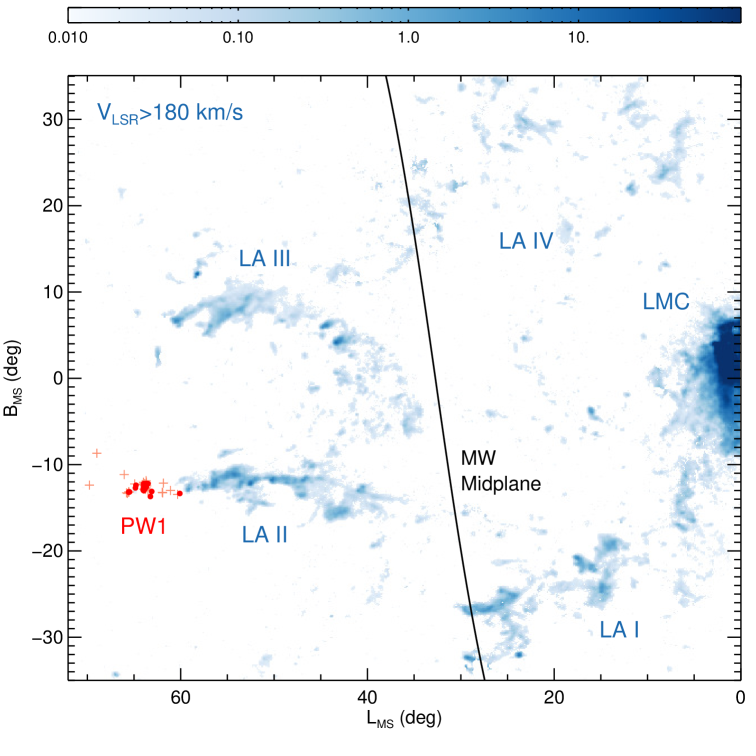
Figure 1: Map of the Leading Arm region. The GASS HI column density (in units of 10¹⁹ atoms cm^-2) is shown in blue with the LA I-IV and LMC labeled. The 28 PW1 stars for which we obtained MIKE spectra shown as filled red circles while the light-red crosses are 43 additional PW1 candidates based on photometry and Gaia DR2 proper motions. The MW midplane is shown by a solid black line.

While the initial claims of LA-associated young stars were invalidated with Gaia DR2 proper motions, Price-Whelan et al. (2018, hereafter Paper I) discovered a young stellar association (“Price-Whelan 1”; hereafter PW 1) using Gaia proper motions in the vicinity of the LA. In Paper I, PW 1 was found to be young, metal-poor, and likely disrupting with a sky position similar to that of LA II. By comparing to stellar evolution models, Paper I measured an age of $\sim$116 Myr, distance of $\sim$29 kpc, metallicity of [Fe/H] = $-$1.14, and total present-day stellar mass of $\sim$1200 $\textrm{M}_{\odot}$. Although the radial velocity (RV) of the cluster was unknown at the time, the range of possible orbits strongly suggested an association with the MCs and a passage through the outer MW disk $\sim$116 Myr ago. However, there are many HI structures in the vicinity of PW 1 (Figure 1), each with a unique RV signature. Associating PW 1with a particular gaseous substructure therefore requires spectroscopic RV measurements of the cluster stars.

In this paper, we analyze the stellar parameters and mean kinematics of the stars in PW 1 to better constrain the properties and origin of this young stellar association. We also use the kinematics of PW 1 in an orbital analysis to constrain the density of the MW hot halo and outer gas disk. The layout of the paper is as follows: Section 2 describes the observations and data reduction. In Section 3, we present the procedures for deriving radial velocities and stellar parameters. Our main results are detailed in Section 4 and discussed in Section 5. Finally, our main conclusions are summarized in Section 6.

2 Observations and Reductions

We obtained spectra for the brightest 28 PW 1 stars and 6 standard stars using the Magellan Inamori Kyocera Echelle (MIKE) spectrograph (Bernstein et al., 2003) on Magellan-Clay at Las Campanas Observatory on 25, 26, and 30 April and May 1 2019. Some of the stars were also observed on 26, 27, 28 December 2018 using the Goodman Spectrograph (Clemens et al., 2004) at the SOAR Telescope with consistent results. Table 1 presents the names, coordinates, magnitudes, signal-to-noise ratio (S/N) and proper motions for each target. Figure 2 shows their location in a Gaia color-magnitude diagram (red open circles) relative to all PW 1 candidates (blue) and field stars (black). Observations were taken with the 0.7^′′ slit and 2x2 pixel binning, such that the native resolution for each spectrum is $R=31,000$. Exposure times ranged from 70 to 1060 seconds under generally good conditions with an average seeing of 0.7^′′. A the native MIKE resolution, S/N per resolution element (3.15 pixels) for the PW 1 stars is 10–24 with a median of $\sim$18, although the S/N per pixel is increased by 3.16$\times$ by rebinning the 1-D extracted spectra (see below). Six of the stars have low S/N due to moderately cloudy conditions (PW1-00 – PW1-05) and are generally excluded from detailed analysis. An additional high-S/N spectrum was obtained for PW1-00 (the brightest PW 1 member) that is suitable for precise chemical abundance work, but this analysis is reserved for future work.

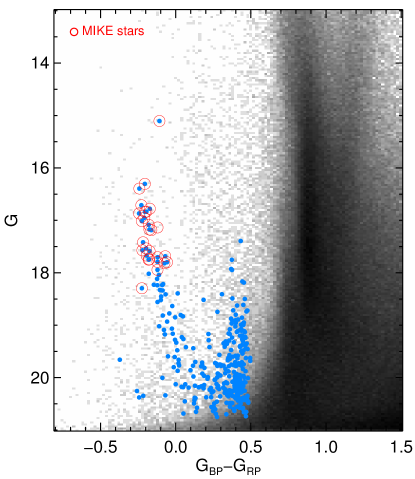
Figure 2: Color-magnitude diagram using Gaia photometry in the vicinity of PW 1(black points); the specific spatial constraints are 173.5${}^{\circ}~{}$$<$ $\alpha$ $<$ 185.5°, $-$35.0${}^{\circ}~{}$$<$ $\delta$ $<$ $-$23.0°. Filled (blue) circles are probable PW 1 members (with $G_{\rm BP}-G_{\rm RP}<0.5$) based on the proper motion model described in Paper I. MIKE spectra were obtained for the 28 stars indicated by open red circles, including PW1-03 which was not used in the analysis due to low S/N.

Figure 3: Three example MIKE blue-arm spectra. The top two panels show example PW 1 stars, PW1-06 (s/N=29) and PW1-07 (S/N=30) , while the bottom panel is the reference star HD146775 (S/N=826).

The observations were processed using the MIKE pipeline, which is part of the CarPy spectroscopic reduction package that uses algorithms described in Kelson et al. (2000) and Kelson (2003). The MIKE pipeline performs image processing (bias removal, flat fielding) as well as extracting the spectra, determining a wavelength solution, subtracting the sky, and co-adding multiple exposures of single objects. The multi order reduced spectra were then merged into a single spectrum and normalized using the IRAF tasks continuum and scombine. While MIKE produces spectra from the blue and red arms, only blue spectra with a wavelength range of 3550–5060Å were used in our analysis. Figure 3 shows example spectra for two PW 1 stars and the standard star HD 146775.

Finally, the full MIKE resolution was significantly higher than needed for our science goals. Therefore, we rebinned the spectra with a bin size of 10 native MIKE pixels which increased the S/N per pixel by $\sim$3.16$\times$. This had little impact on the spectral features as they are already quite broad in these hot, B-type stars.

3 Data Analysis

3.1 Radial Velocities

A RV was determined for each star via a two phase process. First, we determine an initial RV for each source by cross-correlating the unsmoothed MIKE spectra (excluding the region below 3665Å) with a hot synthetic stellar spectrum having stellar parameters ($\rm T_{eff}$, $\log{g}$, [Fe/H]) = (15,000K, 4.0, $-$1.0) and set to the the resolution and logarithmic wavelength scale of the MIKE spectra. Second, the RVs were then redetermined using its best-fit model as the cross-correlation template after the star-by-star stellar parameters were determined following the procedure described in §3.2. The second iteration provided similar, but more precise and accurate RV solutions.

We determine the RV uncertainties using a Monte Carlo scheme. Mock observations were generated for each star by adding Gaussian noise similar to that observed in the science spectrum to its best-fit model spectrum. One hundred mock observations were generated for each star, the RV determined for each with the method described above, and the uncertainty calculated as the robust standard deviation of these values. The typical RV uncertainty from this procedure is $\sim$3 km s${}^{-1}~{}$but the uncertainty increases roughly with the inverse of S/N.

We compared our RVs for the six bright standard stars to literature values and find a median offset of $-$2.0 km s^-1, which is consistent within the uncertainties of our measurements.

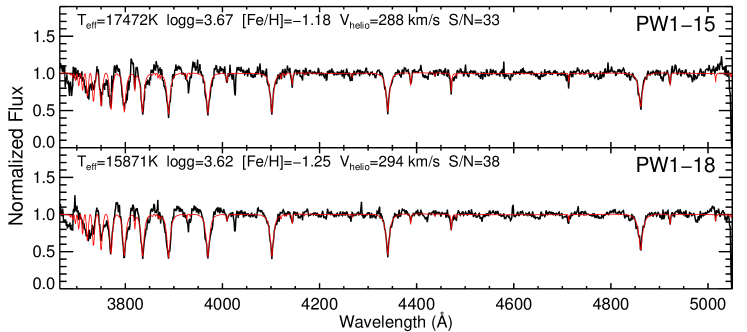
Figure 4: Example best-fit spectra from The Cannon. MIKE spectra for PW1-15 and PW1-18 (black) are shown with the best-fit Cannon models overlaid (red). These show excellent agreement. The best-fit stellar and RV parameters are noted in the top left corner for each star.

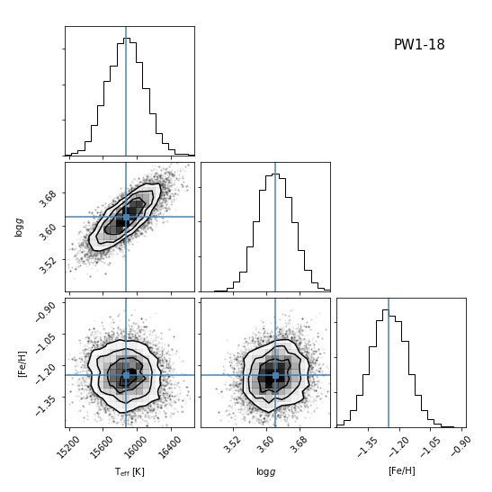
Figure 5: An example corner plot showing the emcee MCMC posterior distributions for PW1-18. The median values are shown by the blue lines.

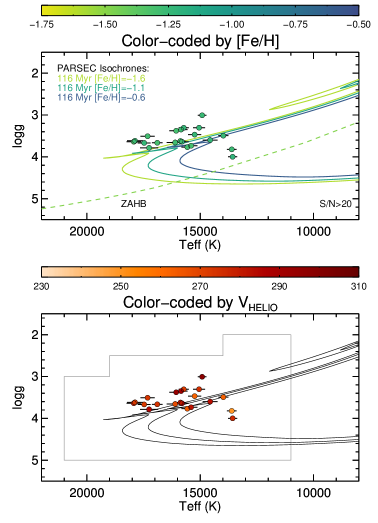
Figure 6: Stellar parameters determined from The Cannon for the 21 PW 1 stars with S/N$\geq$20 and compared to PARSEC isochrones. The top panel shows $\log{g}$ vs. $\rm T_{eff}$ color-coded by [Fe/H] whereas the bottom shows the same points color-coded by $V_{\rm hel}$. As indicated by color coding in the top panel, the isochrones have an age of 116 Myr and a metallicity of [Fe/H] = $-$1.6, $-$1.1 and $-$0.6 dex, respectively. The [Fe/H]=$-$1.48 Zero-Age Horizontal Branch (ZAHB) from Dorman et al. (1993) is also shown as a dashed line. The boundary of the synthetic spectral grid used in The Cannon analysis is shown in light gray in the bottom panel.

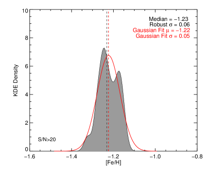
Figure 7: Kernel Density Estimate (KDE) of the distribution of [Fe/H] measurements for 21 PW 1 stars with S/N$\geq$20 and a bandwidth of 0.04 dex, which is smaller than the typical [Fe/H] uncertainty of $\sim$0.10 dex. A single Gaussian model is fit to the histogram and has peak at $-$1.22 and $\sigma$ of 0.05 dex. The median [Fe/H] is $-$1.23, the standard deviation is 0.06 dex.

3.2 Stellar Parameters

We use The Cannon (Casey et al., 2016; Ness et al., 2015) to determine stellar parameters ($\rm T_{eff}$, $\log{g}$, [Fe/H]) for our 28 spectra. The Cannon is a data-driven model for stellar spectra in which the stellar flux (at a given wavelength) is parameterized as a polynomial function of stellar parameters and abundances (i.e., “labels”). A Cannon “model“ is trained on a set of spectra (observed or synthetic) with well-known labels (i.e., the “training set”) and can then be used to determine the labels for other spectra. An advantage of this method is that it exploits at the information available in the spectra and is also fully automated. First, we construct a grid of 330 synthetic spectra (at a resolution of 1.5Å) with the Synspec (Hubeny & Lanz, 2011, 2017) spectral synthesis software and IDL wrappers and auxiliary scripts (Allende Prieto, private communication). Given an input atmospheric model, a linelist and stellar parameters and abundances, Synspec solves the radiative transfer equation over a specified wavelength range and resolution resulting in a synthetic spectrum. We use the Kurucz LTE atmospheric models and include both atomic and molecular lines. For the spectral grid, the $\rm T_{eff}$ ranges from 11,000K to 21,000K in steps of 1,000K, the $\log{g}$ ranges from 2.0 to 5.0 in steps of 0.5 dex, and the [Fe/H] ranges from $-$1.5 to $+$0.5 in steps of 0.25 dex (the boundary of the grid is shown in the bottom panel of Figure 6). The synthetic spectra were interpolated onto the wavelength grid of the final MIKE spectra and normalized. For The Cannon model, we used a quadratic polynomial model to represent how the flux varies with the three stellar parameters at each wavelength. To provide a simple sanity check of the model generated by The Cannon, we determined the stellar parameters for the training set spectra using The Cannon model and compared these results to the training set input parameters. We found no significant biases. Specifically, the $\rm T_{eff}$ had an offset of 0.5K and scatter of $\sigma$=250K, $\log{g}$ had a mean offset of $-$0.003 dex and $\sigma$=0.06 dex, while [Fe/H] had no offset with a scatter of $\sigma$=0.12 dex.

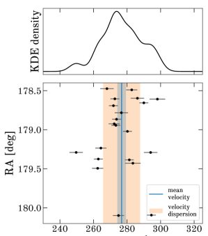
Figure 8: Top panel: Kernel density estimate of the distribution of RV measurements with a bandwidth $b=3~{}\mbox{km s${}^{-1}$}$. Bottom panel: Individual RV measurements for PW 1 stars with uncertainties (black markers and error bars) as a function of right ascension (RA). The solid line (blue) shows the inferred mean RV of PW 1, and the shaded (blue) region shows the uncertainty on the mean RV, $276.7\pm 2.5~{}\mbox{km s${}^{-1}$}$. The larger shaded region (orange) shows the median posterior value of the velocity dispersion of PW 1, $11.0\pm 2~{}\mbox{km s${}^{-1}$}$.

We use the initial stellar parameters determined with The Cannon to refine the normalization of the MIKE spectra using a scaling factor determined by the ratio of the observed spectrum divided by the best-fit Cannon spectrum with heavy Gaussian-smoothing (FWHM = 38Å). New Cannon solutions were then found for these “renormalized” observed spectra. Two example fits from The Cannon are shown in Figure 4 in comparison to their best-fit Cannon model and its parameters.

We use the emcee (Foreman-Mackey et al., 2013; Goodman & Weare, 2010) MCMC sampler to determine the stellar parameters for each star and their uncertainties. We run with 30 walkers for 1000 step and the first 200 are discarded as “burn-in” steps. Figure 5 shows an example “corner” plot of the posterior distributions for PW1-18 and the median values with the blue lines. Typical statistical uncertainties are $\sim$300K in $\rm T_{eff}$, 0.06 dex in $\log{g}$, and 0.10 dex in [Fe/H].

Figure 6 shows the distribution of $\log{g}$ vs. $\rm T_{eff}$ color-coded by [Fe/H] and $V_{\rm LSR}$ in comparison to PARSEC isochrones. We note that one or two stars (including PW1-13) might be hot horizontal branch (HB) stars based on the best-fit $\log{g}$ and $\rm T_{eff}$ (e.g., Zhang et al., 2019). Confirming whether a star is either on the HB or MS evolutionary stage is beyond the scope of this paper due to the lack of He abundance information. However, we emphasize that inclusion of a few potential HB stars does not affect our dynamical analysis and main conclusions because all the stars in our sample share consistent proper motions and radial velocities.

Figure 7 shows the resulting [Fe/H] distribution of PW 1 stars, which is peaked at [Fe/H] $\approx$ $-$1.23 and has a dispersion of 0.06 dex. This spectroscopically-measured metallicity is in good agreement with our photometry-based metallicity measurement of [Fe/H]=$-$1.1 in Paper I. The small dispersion of the PW 1 [Fe/H] values suggests that our uncertainties might be overestimated and that our true uncertainties are closer to $\sim$0.05 dex. The derived stellar parameters and their uncertainties are also provided in Table 1.

4 Results

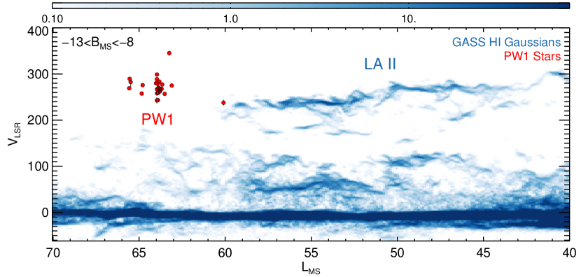
Figure 9: Position–velocity diagram of the PW 1 stars compared to the GASS HI data (McClure-Griffiths et al., 2009). The background bluescale image is the integrated intensity of the GASS Gaussian centers summed along $B_{\rm MS}$ in units of 10¹⁸ atoms cm^-2 degree The tip of LA II has a velocity of $\sim$233 km s^-1. Each PW 1star is plotted at its determined $V_{\rm LSR}$as a red filled circle with its uncertainty. The stars have a mean velocity of $\sim$273.4 km s${}^{-1}~{}$, slightly higher than but similar to the gas in LA II.

4.1 PW 1 Velocity

With proper motion and radial velocity information for individual stars in PW 1, along with a constraint on the mean distance to PW 1 (Paper I), we construct a simple model for its internal velocity structure to infer the true mean velocity and velocity dispersion from these projected quantities. We use the $N=22$ (out of 28) stars with spectroscopic $\textrm{S}/\textrm{N}\geq 10$ for this analysis.

We assume that the 3-D velocity of each $n$ star, $\boldsymbol{v}_{n}$, is drawn from a 3D Gaussian with mean $\boldsymbol{v}_{0}$ and a diagonal covariance matrix $\mathbf{C}=\sigma_{v}^{2}\,\mathbb{I}_{3}$, where $\sigma_{v}$ is the (assumed isotropic) velocity dispersion, and $\mathbb{I}_{3}$ is the identity matrix. For each individual star, we only observe projected or astrometric quantities, like sky position $(\alpha,\delta)$, distance $d$, proper motions $(\mu_{\alpha},\mu_{\delta})$, and radial velocity $v_{r}$. We assume that the sky position of each star is known with infinite precision, the observed distance is unresolved and given by the mean cluster distance and uncertainty (Paper I), the proper motions are given by Gaia with a 2D covariance matrix $\mathbf{C}_{\mu}$, and the radial velocities are measured in this work. The (unobserved) true 3D velocity of each star, drawn from the model given above, is related to the observed astrometric quantities through a projection matrix that depends on sky position (see, e.g., the appendix of Oh et al. 2017). The full model therefore has $N+3\,N+3+1=92$ parameters: the true distance to each star, the true 3D velocity vector of each star, the mean velocity of PW 1, and the velocity dispersion. This model is implemented in the Stan (Carpenter et al., 2017) probabilistic programming language, and we use the built-in No-U-Turn Hamiltonian Monte Carlo sampler (Homan & Gelman, 2014) to generate posterior samples over all of the model parameters. We run the sampler for 4000 steps in total for 4 independent Markov Chains: 2000 burn-in and tuning steps (that are discarded), and then a further 2000 steps for each chain, from which we assess convergence by computing the effective sample size and Gelman-Rubin convergence statistic for each chain.

Given the posterior samples generated as described above, we measure a mean barycentric radial velocity for PW 1 of $276.7\pm 2.5~{}\mbox{km s${}^{-1}$}$ and mean proper motion of $(-0.52,0.42)\pm(0.04,0.03)~{}\textrm{mas}\,\textrm{yr}^{-1}$. Assuming a total solar velocity of $(11.1,220+12.24,7.25)~{}\mbox{km s${}^{-1}~{}$}$ (Schönrich et al., 2010), this corresponds to a Galactocentric (Cartesian) velocity for PW 1 of $v_{\textrm{galcen}}\approx(0.6,2.2,186)~{}\mbox{km s${}^{-1}$}$. We find a velocity dispersion of $\sigma_{v}=11.0\pm 2~{}\mbox{km s${}^{-1}$}$, which is consistent with a robust standard deviation computed from the RVs alone (§3.1), indicating that the constraint on the velocity dispersion comes predominantly from the RV data in this work. Figure 8 shows the individual RV measurements of each observed PW 1 star (black points) as a function of right ascension, along with the inferred mean velocity (blue) and velocity dispersion (orange).

In the sections to follow, we compare the inferred line-of-sight velocity of PW 1 with HI radio data (e.g., from GASS) where it is necessary to convert to the “kinematic local standard of rest” (LSRK), which historically uses the average of Solar neighborhood star velocities (Delhaye, 1965; Gordon, 1976). In this reference frame, the mean velocity is $V_{\rm LSR}=273.4\pm 2.5~{}\mbox{km s${}^{-1}$}$.

4.2 Leading Arm Origin

Figure 9 shows the position–velocity diagram of the PW 1 stars and the HI gas (GASS; McClure-Griffiths et al., 2009) using the Gaussian decomposition techniques described in Nidever et al. (2008). The mean $V_{\rm LSR}$ velocity of 273.4 km s${}^{-1}~{}$of the PW 1 stars is very similar to the velocity of the LA II gas of 233 km s^-1. Absorption-line studies of the LA HI find a value of [Fe/H]$\sim$-1 dex (Lu et al., 1998; Fox et al., 2018; Richter et al., 2018), which is similar to the mean metallicity of PW 1 stars studied here of [Fe/H]$\sim$–1.23 dex (see Figure 7). Therefore, we conclude that the PW 1 stars are physically associated with the LA II gas based on their similar RVs and metallicities.

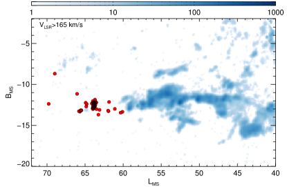
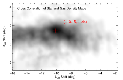
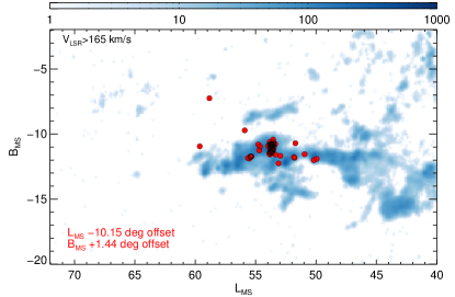
Figure 10: The spatial distribution of the HI gas and 71 PW 1 candidate stars based on photometry and Gaia DR2 proper motions. (top) The gas and PW 1 stars at their current ($L_{\rm MS}$,$B_{\rm MS}$) positions. (middle) The 2D cross-correlation map of the star and gas density maps with the shift of ($-$10.15°,$+$1.44°) in ($L_{\rm MS}$,$B_{\rm MS}$). (Bottom) PW 1shifted by the offset determined in the cross-correlation.

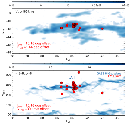
Figure 11: Spatial and Position–velocity diagram for the 28 PW 1 stars with radial velocities and LA II gas. The top panel shows the positions of the PW 1 stars (red filled circles) and the LA II gas after the cross-correlation offset has been applied (see Figure 10). The bottom panel shows the same spatially-offset stars in position-velocity space. A $V_{\rm LSR}$ offset of 30 km s${}^{-1}~{}$has been applied such that the stars align with the densest portions of the LA II gas.

4.3 Spatial Offset between Stars and Gas

The current location of PW 1 is close to LA II on the sky, but there is little gas in its immediate vicinity in the position-velocity diagram (Figure 9). The top panel of Figure 10 shows the spatial offset between PW 1 and the LA II gas in the MS coordinate system ($L_{\rm MS}$,$B_{\rm MS}$). The gas from which PW 1 originated should experience ram pressure from the MW hot halo gas (e.g., Mastropietro et al., 2005). Because the stars will not feel this force, the gas and stars will decouple over time with the net effect that the gas trails the stars in their orbit. With this in mind, it is not surprising that there is little gas in the immediate vicinity of PW 1. Thus, the spatial offset does not rule out LA II as the origin gas for PW 1.

Quantitatively, the magnitude of the spatial decoupling between the stars and gas is determined by a 2D cross-correlation of the star and gas maps (Figure 10, top). The individual maps were masked such that only the highest density regions were used. The result of the cross-correlation is in the middle panel of Figure 10. The peak of the cross-correlation is at an offset of ($-$10.15°,$+$1.44°) in ($L_{\rm MS}$,$B_{\rm MS}$), which is indicated as a red cross in the middle panel of Figure 10. The bottom panel of Figure 10 shows that shifted PW 1 positions are well aligned with the high-density peaks of the HI gas. These shift positions are more representative of the original relative positioning of the gas forming PW 1 within the LA II complex.

Figure 11 shows a slightly different visualization of this process. The top panel of Figure 11 zooms into the ($L_{\rm MS}$,$B_{\rm MS}$) region around the position-shifted stars with $V_{\rm LSR}$ measurements. Ram pressure will also act to modify the velocities of the gas it acts on, and thus an exact match between the velocities of the birth-gas and resulting stars is not expected. The bottom panel of Figure 11 is the resulting velocity-position diagram; a 30 km s${}^{-1}~{}$velocity offset is required to have the PW 1 stars align with the densest portions of the gas in position-velocity space. We will use this offset in the next section to place a constraint on the halo gas driving the ram pressure effects.

4.4 Ram Pressure

If the spatial and velocity offsets between this gas and PW 1 are indeed due to a roughly constant ram pressure, then the measured position-velocity offsets become a means of inferring the properties of the gas performing the ram pressure. In particular, we place a constraint on the average density of the “hot” MW-halo gas, a medium that remains difficult to characterize directly (for an overview see Putman et al., 2012).

At a distance of 29 kpc, the angular offset of 10.15${}^{\circ}~{}$corresponds to a tangential distance of $\sim$5.14 kpc. Over 116 Myr that corresponds to a mean “drift” velocity of $\sim$43.3 km s${}^{-1}~{}$or a deceleration of $\sim$0.747 km s^-1 Myr^-1. The total change in the tangential velocity of the gas over this period is $\sim$86.6 km s^-1. The $V_{\rm LSR}$ of LA II “tip” is lower than that of PW 1 by $\sim$30 km s^-1. The smaller $V_{\rm LSR}$ shift would indicate that a significant fraction of the deceleration occurred in the tangential direction.

If we assume that ram pressure is the main factor in causing the gas and stars to drift apart and that this is dominated by a roughly constant ram pressure from the MW hot halo, then we can estimate the density of the MW hot halo gas as follows. The ram pressure experienced by the PW 1 “birth cloud” (BC) in LA II is defined as,

$$P=\rho_{\rm MW}~{}v_{\rm BC}^{2},$$ (1)

where $\rho_{\rm MW}$ is the density of the MW halo gas and $v_{\rm BC}$ is the birth cloud velocity through the medium. If $l_{\rm BC}$ is the approximate diameter of the birth cloud, then the acceleration that it experiences ($a_{\rm BC}$) is,

$$a_{\rm BC}\approx\frac{\rho_{\rm MW}~{}v_{\rm BC}^{2}~{}l_{\rm BC}^{2}}{\rho_{\rm BC}~{}l_{\rm BC}^{3}}\approx\frac{\rho_{\rm MW}~{}v_{\rm BC}^{2}}{\rho_{\rm BC}~{}l_{\rm BC}}.$$ (2)

Solving Equation 2 for the ratio of gas density between the MW and the birth cloud gives

$$\frac{\rho_{\rm MW}}{\rho_{\rm BC}}\approx\frac{a_{\rm BC}~{}l_{\rm BC}}{v_{\rm BC}^{2}}.$$ (3)

If we assume that the birth cloud was undergoing a roughly constant deceleration due to ram pressure since forming PW 1, then we can estimate this deceleration from the age of PW 1 ($\Delta{\rm t}$ = 116 Myr) and the spatial offset ($\Delta{\rm x}$ = 10.15${}^{\circ}~{}$= 5.14 kpc), as

$$a_{\rm BC}\approx\frac{2\Delta{\rm x}}{\Delta{\rm t}^{2}}.$$ (4)

This results in $a_{\rm BC}\approx$ 0.747 km s^-1 Myr^-1. The angular width (full-width at half-maximum in $B_{\rm MS}$) of the LA II PW 1 birth cloud from GASS is 0.75${}^{\circ}~{}$or 0.38 kpc. Using this as an approximation of the diameter of the birth cloud ($l_{\rm BC}$) and $v_{\rm BC}$ $\approx$ 235 km s^-1, we obtain $\rho_{\rm MW}/\rho_{\rm BC}$ $\approx$ 0.00505 or that the MW gas density is $\sim$0.5% of that of the PW 1 birth cloud.

We measure the average current column density of the PW 1 birth cloud from the HI GASS data as $N_{\rm H\small{I}}$ $\approx 1.5\times 10^{20}$ atoms cm^-2. Assuming a distance of 29 kpc and a width of $\sim$0.38 kpc gives a number density of $n_{\rm BC}\approx$ 0.128 atoms cm^-3.

Finally, we derive the number density of the hot MW halo as $n_{\rm MW}\approx$ 6.46 $\times 10^{-4}$ atoms cm^-3. This rough estimate of the hot MW halo gas density is an order of magnitude higher than that predicted by the Miller & Bregman (2013) model which gives $\sim$4$\times$10^-5 atoms cm^-3 at this location. However, our estimate here is too simplistic for a number of reasons: (i) we are seeing an integrated effect over the orbit of PW 1, which has passed through higher densities closer to the midplane, and (ii) we consider only a single medium – the hot halo – completely ignoring the impact of the midplane and outer gas disk itself. That this simple estimate is within an order-of-magnitude of state-of-the art measurements motivates the more complex and nuanced simulations that are presented in the next sub-section.

4.5 Ram pressure orbit analysis

The offsets in sky position and velocity between the PW 1 stars and the LA II gas suggest that the gas was likely subject to a drag force or dissipated orbital energy: The offset in position is primarily along the direction of motion, and the gas velocity is slightly lower than that of PW 1. Moreover, the order-of-magnitude computations presented in the previous sub-section suggest that ram pressure from the hot halo produce effects on par with what is seen, albeit more complex interactions of the mid-plane are ignored. We therefore perform a set of orbit integrations to see if the observed position-velocity offsets can plausibly be explained by gas drag from the MW halo when the full orbital motion and influence of the midplane are included.

We use the MW mass model implemented in gala (Bovy, 2015; Price-Whelan, 2017) as the background gravitational potential, and include a time-dependent mass component to represent the LMC. In detail, we represent the mass distribution of the LMC using a Hernquist profile (Hernquist, 1990), which generally follows the the approach used in Erkal et al. (2019), except that we use a total mass of $M_{\rm LMC}=2.5\times 10^{11}~{}\textrm{M}_{\odot}$ (Laporte et al., 2018). We compute the position of the LMC at any given time by integrating the orbit of the LMC center-of-mass backwards from its present day phase-space position (using initial conditions from Patel et al. 2017). We neglect any back-reaction or response of the MW to the presence of the LMC. We use this time-dependent mass model along with the measured position and velocity of PW 1 to numerically integrate the orbit of the PW 1 backwards in time from present day ($t_{2}=0$) to its birth time ($t_{1}=-\tau=-116~{}{\rm Myr}$). We use the Dormand-Prince 8th-order Runge-Kutta scheme (Dormand & Prince, 1980) to numerically integrate these orbits.

Once the phase-space coordinates of PW 1 at its birth time are estimated, we then integrate forward in time, now including the effects of gas drag and momentum coupling between the MW disk and the LA II gas as it crosses the Galactic midplane. We compute the drag acceleration on the gas as

$$\boldsymbol{a}_{\rm drag} =n_{\rm MW}(\boldsymbol{x})\,|\boldsymbol{v}|^{2}\,\Sigma_{\rm LA}^{-1}\,\times\,-\frac{\boldsymbol{v}}{|\boldsymbol{v}|}$$ (5)

where $n_{\rm MW}(\boldsymbol{x})$ is the number density of MW gas at position $\boldsymbol{x}$, $\boldsymbol{v}$ is the orbital velocity, and $\Sigma_{\rm LA}$ is the surface density of the LA gas (following, e.g., Vollmer et al., 2001). For the gas density, we use the gaseous halo model from Miller & Bregman (2013) and the disk model from Kalberla & Kerp (2009) with a Gaussian density profile in the height above the midplane $z$ such that

$$n_{\rm MW}(\boldsymbol{x}) =n_{\rm halo}(r)+n_{\rm disk}(R,z)$$ (6)

$$n_{\rm halo}(r) =n_{0,h}\,\left[1+\left(\frac{r}{r_{c}}\right)^{2}\right]^{-3\beta/2}$$ (7)

$$n_{\rm disk}(R,z) =n_{0,d}\,e^{-\frac{R-R_{\odot}}{R_{n}}}\,e^{-\frac{1}{2}\,\frac{z^{2}}{\sigma_{z}(R)^{2}}}$$ (8)

$$\sigma_{z}(R) =0.85\,h_{0}\,e^{\frac{R-R_{\odot}}{R_{0}}}$$ (9)

where $r$ is the spherical radius, $R$ is the cylindrical radius, $R_{\odot}=8.1~{}\textrm{kpc}$ is the solar Galactocentric radius, and all parameter values are taken from Kalberla & Kerp (2009). We assume that the surface density of the PW 1 birth cloud in LA II starts with $\Sigma_{0}\approx 50~{}\textrm{M}_{\odot}~{}\textrm{pc}^{-2}$ (comparable to other LMC molecular clouds Wong et al., 2011) and ends (at present day) with a surface density equal to the measured column density of the LA II region, $\Sigma_{f}\approx 0.56~{}\textrm{M}_{\odot}~{}\textrm{pc}^{-2}$ such that

$$\Sigma_{\rm LA}(t)=\exp\left[\frac{(\ln\Sigma_{f}-\ln\Sigma_{0})}{\tau}\,t+\ln\Sigma_{f}\right]$$ (10)

where again $\tau$ is the age of PW 1, $t_{1}=-\tau$, and $t_{2}=0$.

As mentioned above, we also allow for momentum coupling between the MW disk and the LA II gas as it passes through the Galactic midplane. To take this momentum coupling into account, we add an additional acceleration to the orbit integration, $\boldsymbol{a}_{\rm coupling}$, defined to point in the direction of Galactic rotation such that

$$\boldsymbol{a}_{\rm coupling}=\alpha\,\hat{\boldsymbol{v}}_{rot}(\boldsymbol{x})\,e^{-\frac{1}{2}\,\frac{z^{2}}{\sigma_{z}(R)}}$$ (11)

where $\alpha$ is a free parameter that determines the magnitude of the coupling, $\hat{\boldsymbol{v}}_{rot}(\boldsymbol{x})$ is a unit vector that points in the direction of Galactic rotation at the position $\boldsymbol{x}$, and the Gaussian in height, $z$, makes this operate only when the gas orbit is close to the Galactic plane.

We next allow the scale densities, $n_{0,h}$ and $n_{0,d}$, and the momentum coupling parameter, $\alpha$, to vary and fit for the values of these parameters that best reproduce the observed position and velocity offsets between PW 1 and the LA II gas. We define a fiducial point in $L_{\rm MS}$, $B_{\rm MS}$, $V_{\rm hel}$ to set the present-day location of the densest LA II gas (see Section 4.3) that could have plausibly formed PW 1:

$$L_{\rm MS} =53.7^{\circ}$$ (12)

$$B_{\rm MS} =-11.1^{\circ}$$ (13)

$$V_{\rm hel}~{} =239~{}\mbox{km s${}^{-1}$}\quad.$$ (14)

We construct a likelihood function using the above orbit integration scheme and evaluate the likelihood of the present-day (i.e. final) orbit phase-space coordinates relative to the fiducial point defined previously. We assume a Gaussian tolerance of $\sigma_{\rm LB}=0.5^{\circ}$ for $L_{\rm MS}$ and $B_{\rm MS}$, and $\sigma_{v}=1~{}\mbox{km s${}^{-1}$}$ for $V_{\rm hel}$ and evaluate the likelihood as

$$3p(L_{\rm MS},B_{\rm MS},V_{\rm hel} \,|\,n_{0,h},n_{0,d},\alpha)=$$

$$\mathcal{N}(\textrm{L}_{\rm orbit}\,|\,L_{\rm MS},\sigma^{2}_{\rm LB})$$

$$\times \mathcal{N}(\textrm{B}_{\rm orbit}\,|\,B_{\rm MS},\sigma^{2}_{\rm LB})$$

$$\times \mathcal{N}(V_{\rm orbit}\,|\,V_{\rm hel},\sigma^{2}_{v})$$ (15)

where $\mathcal{N}(\cdot\,|\,\mu,\sigma^{2})$ represents the normal distribution with mean $\mu$ and variance $\sigma^{2}$. In practice, we implement this function (programmatically) over the log values of the three parameters (because they must be positive), but we assume uniform priors in the parameter values over the domain $(a,b)=(e^{-30},e^{5})$ for each parameter such that the prior distribution is

$$p(n_{0,h},n_{0,d},\alpha)=\mathcal{U}(n_{0,h}\,|\,a,b)\,\mathcal{U}(n_{0,d}\,|\,a,b)\,\mathcal{U}(\alpha\,|\,a,b)$$ (16)

where $\mathcal{U}(\cdot\,|\,a,b)$ is the uniform distribution defined over the domain $(a,b)$.

We first optimize the log-posterior,

$$\ln p(n_{0,h},n_{0,d},\alpha \,|\,L_{\rm MS},B_{\rm MS},V_{\rm hel})\propto$$

$$\ln p(L_{\rm MS},B_{\rm MS},V_{\rm hel}\,|\,n_{0,h},n_{0,d},\alpha)$$

$$+ \ln p(n_{0,h},n_{0,d},\alpha)$$

using the BFGS algorithm (implemented in scipy, Byrd et al., 1995; Jones et al., 2001–) and then we use these optimal parameter values as initial conditions to run a Markov Chain Monte Carlo (MCMC) sampling of the posterior probability distribution (pdf) of our parameters. We use an affine-invariant, ensemble MCMC sampler (emcee; Foreman-Mackey et al., 2013; Goodman & Weare, 2010); we run with 64 walkers for 512 “burn-in” steps (that are discarded) and then run for an additional 1024 steps. We thin the resulting chains by taking every 4th step, and combine the parameter samplings from all thinned chains. Figure 12 shows histograms of posterior samples transformed into values of the halo gas density evaluated at the orbital pericenter, $n_{\rm halo}(17~{}\textrm{kpc})$, and the disk gas density at the midplane at $n_{\rm disk}(20~{}\textrm{kpc},0)$. The posterior values of the coupling coefficient, $\alpha$, were all $<e^{-12}$ and thus consistent with zero.

The best-fit parameters require a somewhat larger halo and disk gas densities than the fiducial MW gas density models from Miller & Bregman (2013) and Kalberla & Kerp (2009). In detail, we find

$$n_{\rm halo}(17~{}\textrm{kpc}) =2.7_{-2.0}^{+3.4}\times 10^{-3}~{}{\rm atoms}~{}{\rm cm}^{-3}$$ (17)

$$n_{\rm disk}(20~{}\textrm{kpc},0) =6.0_{-2.0}^{+1.5}\times 10^{-2}~{}{\rm atoms}~{}{\rm cm}^{-3}$$ (18)

as compared to the fiducial values $n_{\rm halo,M13}(17~{}\textrm{kpc})=1.2\times 10^{-4}~{}{\rm atoms}~{}{\rm cm}^{-3}$ and $n_{\rm disk,K09}(20~{}\textrm{kpc},0)=2\times 10^{-2}~{}{\rm atoms}~{}{\rm cm}^{-3}$. However, the goal of this analysis is only to illustrate that the observed offsets could plausibly be described by ram pressure, and that the inferred MW halo and disk gas densities needed to explain the magnitude of the ram pressure drag are reasonable. In doing this, we neglect more complex density evolution of the LA gas, assume that the LA II gas, at least around the PW 1 birthplace, acts like a cloud (rather than a dissolving and morphologically-varying gas filament), and assume that no supernovae (SNe) have impacted the orbital energy of the gas. Still, this result motivates more detailed simulation of the interaction between the LA and the MW.

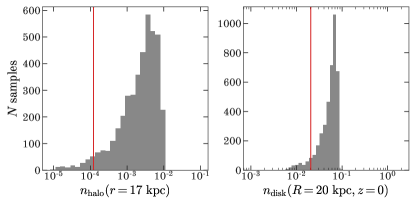
Figure 12: Posterior samples from the ram pressure orbit analysis, transformed to values of the inferred halo gas density at $r=17~{}\textrm{kpc}$ $n_{\rm halo}(17)$ (left panel) and disk gas density (right panel) at the midplane at $(R,z)=(20,0)~{}\textrm{kpc}$, $n_{\rm disk}(20,0)$. Vertical red lines show the values from the default Milky Way model from Miller & Bregman (2013) and Kalberla & Kerp (2009).

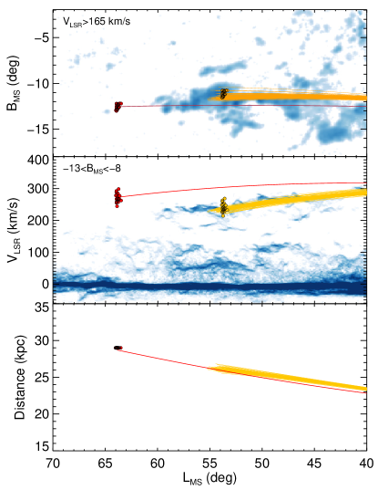
Figure 13: The orbits of both the mean PW 1 stars and the originating gas that experienced ram pressure. (Top) $B_{\rm MS}$ vs. $L_{\rm MS}$, (middle) $V_{\rm LSR}$ vs. $L_{\rm MS}$, and (bottom) distance vs. $L_{\rm MS}$. The red line is the PW 1 orbit with no ram pressure, while the orange lines show 64 orbits of the PW 1 birth cloud drawn from the MCMC posterior distributions of the parameters.

5 Discussion

The distance, radial velocity, metallicity, and orbit suggest that not only is PW 1 associated with LA II, but that it is also associated with the MCs and MS. The association of PW 1 with LA II permits a more nuanced view of the LA than has previously been feasible. Not only does PW 1 provide a distance measurement to the LA, but it also constrains its chemical, orbital, and dynamical properties, such as how it is affected by ram pressure from the MW hot halo. At the same time, affiliating PW 1 with the LA gas also explains some of its properties, as discussed below.

5.1 The Spatial Morphology of PW 1

One of the mysteries of PW 1 is its unusual spatial shape and elongated distribution. However, the spatial correlation of the HI LA II gas and the PW 1 stars suggests a natural explanation for this. The PW 1 stars do not represent one single cluster that has disrupted but rather is likely the outcome of multiple star formation events associated with high-density HI clumps in LA II. This is a common feature observed in jellyfish galaxies experiencing ram pressure in galaxy clusters. Therefore, it might be more appropriate to call PW 1 a star formation “complex” or association rather than a star cluster in the traditional sense.

5.2 Origin of the Leading Arm

The mean metallicity of PW 1 of $\approx-1.23$ is similar to the measured metallicity of the LA ([O/H]$\approx$ $-$1.16; Fox et al. 2018), the Magellanic Bridge ($\approx$ $-$1.0; Lehner et al., 2008) and the trailing MS ($\approx$ $-$1.2; Fox et al., 2013a). There is a large range in the measured metallicities of MW HI high-velocity clouds (HVCs; Wakker, 2001), and, therefore, the similarity of the metallicities in these distinct systems supports the notion that the LA, MB, and MS all share a common origin. These metallicities are also consistent with the metallicity of the SMC $\sim$2 Gyr ago. Therefore, all of these gas structures associated with the MCs likely originated mainly from the SMC from the same tidal event about 2 Gyr ago.

Despite the similar metallicities among the gas structures, the origin of the MS and LA are still debated. This is mainly because (1) the observational data is far from complete – e.g., the metallicity measurements are limited to small number of sightlines, and (2) there are some observed features that cannot be easily explained by the sole SMC origin (e.g., Fox et al., 2013b). One of the recent theoretical studies Pardy et al. (2018) argued that both the LMC and SMC contributed to create the LA and MS gas features. However, another recent MS simulation work by Tepper-García & Bland-Hawthorn (2018) suggested that the LA gas does not originate in the MCs because the ram pressure from the MW hot halo gas would prevent the gas from reaching its present position. If PW 1 is indeed affiliated with LA II, as we suggest here, then there is now observational evidence that the impact of ram pressure is overestimated in Tepper-García & Bland-Hawthorn (2018). The key discriminant is the assumed $\rho_{\rm MW}$ in Tepper-García & Bland-Hawthorn (2018) versus what we infer from our scenario for PW 1.

5.3 No Natal Gas Disruption?

The conditions for triggering star formation in the LA is not well understood. Based on the fact that PW 1 is the only known stellar component to date that is likely associated with LA II, the birth cloud of PW 1 must have satisfied very special star formation conditions in the LA while passing through the Galactic midplane. Aside from the unknown star formation conditions of PW 1, there is another mystery: How has the morphology of the PW 1 birth cloud remained mostly intact? Our analysis in §4.3 shows that the present-day spatial distribution of the associated HI gas resembles that of the PW 1 stars across $\sim$2.5 kpc.

A gas cloud that forms a young star cluster is disrupted when the first SN occurs. The SN-explosions effectively act to distort the original spatial correlations between the gas and stars by injecting radiative and mechanical energy into the birth gas. Similar spatial distributions of the stars and gas after the shift of $(-10.15\arcdeg,+1.44\arcdeg)$ in $(L_{\rm MS},B_{\rm MS})$ indicate that PW 1 birth cloud did not undergo significant gas removal and/or gas destruction period at all, or at least not at significant level. This might only be possible in the absence of stellar feedback in the PW 1 birth cloud.

One way to avoid the impact of stellar feedback on the gas cloud is not to have SN events. To test the possibility that no SNe occurred in PW 1, we compute the expected number of SN explosions in PW 1-like star clusters. Based on the present-day mass, age, and metallicity of PW 1, PARSEC stellar evolutionary models suggest that the initial mass of PW 1 is $\sim$1800 $\textrm{M}_{\odot}$. We then simulate a 1800 $\textrm{M}_{\odot}$ star cluster 20000 times assuming a Kroupa IMF and count the number of SN explosion events in each star cluster. If we assume that all stars more massive than 8 $\textrm{M}_{\odot}$ explode as Type II SNe, then all of the simulated PW 1-like clusters produce at least 1 core-collapse SN $\sim$3 Myr (a typical lifetime of a 8 $\textrm{M}_{\odot}$ star) after its birth. Thus, this scenario is unsuitable to explain the similar present-day spatial pattern between the PW 1 and its birth cloud.

Another way to avoid the gas disruption by stellar feedback is to spatially decouple the birth cloud and the newly formed stars before the first SN explosion. Over 3 Myr, the PW 1 stars were able to travel $\sim$14.3 pc (corresponding to $\sim$50 lyr) away from the birth cloud based on the orbital calculation in §4.5. This spatial decoupling due to ram pressure might prevent the PW 1 birth cloud from being significantly disrupted by stellar feedback. If the PW 1 stars and gas were indeed decoupled before the first SN explosion, our assumption about no effect of SN on the stellar motions (§4.5) can be naturally justified.

6 Summary

We have obtained high-resolution Magellan+MIKE spectra of 28 candidates of PW 1, a young stellar association in the region of the Leading Arm. Our sample allows us to draw some important conclusions about the properties and origin of both PW 1 and the Leading Arm:

1. PW 1 has a median metallicity of [Fe/H]=$-$1.23 with a small scatter of 0.06 dex and an inferred velocity of $V_{\rm LSR}=273.4$ km s${}^{-1}~{}$with a dispersion of 11.0km s^-1. The derived stellar parameters ($\rm T_{eff}$, $\log{g}$, [Fe/H]) are consistent with the young, metal-poor isochrone (116 Myr and [Fe/H]=$-$1.1) that was determined in Paper I using photometry for proper-motion selected members.

2. There is a strong correlation between the spatial patterns of the PW 1 stars and the high-density HI clumps of LA II with an offset of ($-$10.15°,$+$1.55°) in ($L_{\rm MS}$,$B_{\rm MS}$) (Figure 10).

3. Due to the similarity of metallicity, velocity, spatial patterns, and the distance of PW 1, we find that PW 1 likely originated from the LA II complex of the Magellanic Stream.

4. The orbit and metallicity of PW 1 and LA II associate them with the Magellanic Clouds and Magellanic Stream, in contrast to some recent claims to the contrary.

5. Using an orbital analysis of the PW 1 stars and the LA II gas, taking into account ram pressure from a MW model, we constrain the halo gas density at the orbital pericenter of PW 1 to be $n_{\rm halo}(17~{}\textrm{kpc})=2.7_{-2.0}^{+3.4}\times 10^{-3}~{}{\rm atoms}~{}{\rm cm}^{-3}$ and the disk gas density at the midplane at $20~{}\textrm{kpc}$ to be $n_{\rm disk}(20~{}\textrm{kpc},0)=6.0_{-2.0}^{+1.5}\times 10^{-2}~{}{\rm atoms}~{}{\rm cm}^{-3}$. We also predict that the current distance of the PW 1 birth cloud in LA II is 27 kpc.

Future work will investigate the detailed chemical abundances of PW 1 and how it compares to the Magellanic Clouds.

=2.0in

Table 1: PW 1 Spectroscopic Results

Name	Gaia ID	RA	DEC	G	GBP-GRP	$\mu_{\rm RA}$	$\mu_{\rm DEC}$	S/N	$V_{\rm LSR}$	$\sigma_{V}$	$\rm T_{eff}$	$\sigma_{\rm T_{eff}}$	$\log{g}$	$\sigma_{\log{g}}$	[Fe/H]	$\sigma_{\rm[Fe/H]}$
	(J2000)			(mag)		(mas yr-1)			(km s-1)		(K)		(dex)		(dex)
PW1-00	3466763224691512064	11:55:31.8	$-$33:09:11.6	15.10	$-$0.11	$-$0.58	0.46	11.8	239.7	7.3	14465	766	2.25	0.12	$-$0.81	0.32
PW1-01	3480054567924428032	11:56:00.4	$-$29:28:48.9	16.30	$-$0.21	$-$0.45	0.42	14.2	257.1	6.7	17326	873	3.38	0.13	$-$0.82	0.32
PW1-02	3480064910205689088	11:56:18.3	$-$29:19:20.8	16.39	$-$0.24	$-$0.85	0.55	12.4	255.3	7.3	16340	1000	3.20	0.16	$-$1.06	0.35
PW1-03	3480053399693321984	11:56:12.0	$-$29:31:44.4	16.71	$-$0.23	$-$0.37	0.50	4.3	298.5	20.0	17436	2041	3.22	0.36	$-$0.33	0.57
PW1-04	3486242378847130624	12:00:11.5	$-$27:59:50.4	16.78	$-$0.17	$-$0.76	0.45	8.8	235.1	11.3	14654	953	3.38	0.19	$-$1.11	0.30
PW1-05	3479870124848931200	11:57:20.8	$-$29:27:45.2	16.84	$-$0.20	$-$0.58	0.55	16.1	262.7	5.3	17534	548	3.76	0.09	$-$1.04	0.18
PW1-06	3479874106283037568	11:56:56.3	$-$29:25:11.6	16.84	$-$0.20	$-$0.71	0.57	29.1	259.0	3.3	15567	263	3.77	0.05	$-$1.25	0.12
PW1-07	3480052712498583424	11:55:46.3	$-$29:33:56.9	16.87	$-$0.24	$-$0.43	0.50	30.6	267.9	2.7	17321	315	3.51	0.05	$-$1.26	0.12
PW1-08	3486167027940903296	11:56:04.8	$-$28:28:38.8	16.95	$-$0.21	$-$0.47	0.59	32.0	274.9	2.7	17930	321	3.64	0.05	$-$1.32	0.10
PW1-09	3480071644714348032	11:55:41.7	$-$29:17:32.5	17.01	$-$0.23	$-$0.53	0.46	29.3	266.9	3.3	17878	350	3.62	0.05	$-$1.24	0.12
PW1-10	3479874690398598784	11:57:09.5	$-$29:21:50.6	17.09	$-$0.18	$-$0.54	0.40	27.2	288.7	4.0	15805	296	3.64	0.06	$-$1.16	0.14
PW1-11	3485879024613971328	11:57:42.5	$-$29:20:32.8	17.14	$-$0.12	0.22	0.42	22.7	278.2	4.7	14561	329	3.60	0.07	$-$1.17	0.15
PW1-12	3480036975738300800	11:53:53.6	$-$29:38:55.3	17.17	$-$0.17	$-$0.49	0.47	23.4	262.4	4.0	16105	372	3.66	0.07	$-$1.25	0.14
PW1-13	3467765189021964544	12:00:18.7	$-$30:14:30.8	17.19	$-$0.16	$-$0.23	0.30	19.9	341.6	5.3	17216	451	4.19	0.07	$-$1.15	0.17
PW1-14	3480121844292017920	11:54:23.4	$-$29:15:42.0	17.42	$-$0.22	$-$0.40	0.44	24.2	280.7	4.0	17254	401	3.78	0.06	$-$1.24	0.14
PW1-15	3480049757560914944	11:54:25.0	$-$29:23:44.4	17.54	$-$0.20	$-$0.50	0.21	32.9	267.2	2.7	17472	283	3.67	0.05	$-$1.18	0.09
PW1-16	3480046557809199616	11:54:46.1	$-$29:25:33.5	17.57	$-$0.22	$-$0.54	0.45	37.7	266.4	2.7	15726	225	3.31	0.04	$-$1.16	0.11
PW1-17	3480070957519575552	11:55:27.6	$-$29:21:43.8	17.59	$-$0.17	$-$0.48	0.27	37.8	268.3	2.7	16894	235	3.66	0.04	$-$1.27	0.08
PW1-18	3479762991184812544	11:57:32.4	$-$30:14:56.6	17.67	$-$0.19	$-$1.00	0.36	38.1	275.9	2.7	15871	218	3.62	0.04	$-$1.25	0.08
PW1-19	3486175647939287680	11:57:29.7	$-$28:29:54.7	17.70	$-$0.12	$-$0.22	0.29	31.5	257.7	2.7	13979	224	3.49	0.05	$-$1.20	0.10
PW1-20	3479873354664338688	11:57:09.4	$-$29:25:47.3	17.69	$-$0.07	$-$0.61	0.37	29.8	244.3	4.0	13609	210	3.82	0.05	$-$1.22	0.10
PW1-21	3486267147922619136	12:00:22.2	$-$27:56:54.3	17.74	$-$0.18	$-$0.43	0.18	31.6	289.6	2.7	16060	303	3.38	0.05	$-$1.28	0.11
PW1-22	3480047141924659456	11:53:57.4	$-$29:30:37.4	17.75	$-$0.18	$-$0.40	0.40	28.5	277.2	3.3	15402	280	3.73	0.05	$-$1.28	0.11
PW1-23	3480049856344140288	11:54:37.3	$-$29:22:36.4	17.80	$-$0.06	$-$0.53	0.61	31.9	284.5	2.7	15845	285	3.35	0.05	$-$1.23	0.12
PW1-24	3485874897149344256	11:57:58.3	$-$29:24:47.2	17.79	$-$0.12	$-$0.51	0.44	29.9	257.2	3.3	15246	291	3.47	0.06	$-$1.19	0.12
PW1-25	3480070510842975104	11:55:07.5	$-$29:21:14.9	17.82	$-$0.08	$-$0.71	0.37	29.3	271.2	4.0	13570	201	4.00	0.05	$-$1.15	0.10
PW1-26	3480122325328358144	11:54:25.7	$-$29:13:24.8	18.30	$-$0.23	$-$0.42	0.45	21.3	292.6	4.7	14914	189	3.01	0.05	$-$1.21	0.02
PW1-27	3486267251001844736	12:00:23.1	$-$27:55:21.8	17.94	$-$0.12	$-$0.89	0.37	29.3	270.0	3.3	15050	264	3.30	0.05	$-$1.18	0.05

References

- Bernstein et al. (2003) Bernstein, R., Shectman, S. A., Gunnels, S. M., Mochnacki, S., & Athey, A. E. 2003, in Proc. SPIE, Vol. 4841, Instrument Design and Performance for Optical/Infrared Ground-based Telescopes, ed. M. Iye & A. F. M. Moorwood, 1694–1704
- Besla et al. (2007) Besla, G., Kallivayalil, N., Hernquist, L., et al. 2007, ApJ, 668, 949
- Besla et al. (2012) —. 2012, MNRAS, 421, 2109
- Bovy (2015) Bovy, J. 2015, The Astrophysical Journal Supplement Series, 216, 29
- Brown et al. (2018) Brown, A. G. A., Vallenari, A., Prusti, T., & de Bruijne, J. H. J. 2018, Astronomy & Astrophysics, doi:10.1051/0004-6361/201833051
- Brueck & Hawkins (1983) Brueck, M. T., & Hawkins, M. R. S. 1983, A&A, 124, 216
- Brüns et al. (2005) Brüns, C., Kerp, J., Staveley-Smith, L., et al. 2005, A&A, 432, 45
- Byrd et al. (1995) Byrd, R. H., Lu, P., Nocedal, J., & Zhu, C. 1995, SIAM J. Sci. Comput., 16, 1190. http://dx.doi.org/10.1137/0916069
- Carpenter et al. (2017) Carpenter, B., Gelman, A., Hoffman, M., et al. 2017, Journal of Statistical Software, Articles, 76, 1. https://www.jstatsoft.org/v076/i01
- Casetti-Dinescu et al. (2014) Casetti-Dinescu, D. I., Moni Bidin, C., Girard, T. M., et al. 2014, ApJ, 784, L37
- Casey et al. (2016) Casey, A. R., Hogg, D. W., Ness, M., et al. 2016, arXiv e-prints, arXiv:1603.03040
- Casey et al. (2012) Casey, A. R., Keller, S. C., & Da Costa, G. 2012, AJ, 143, 88
- Choi et al. (2018a) Choi, Y., Nidever, D. L., Olsen, K., et al. 2018a, ApJ, 866, 90
- Choi et al. (2018b) —. 2018b, ApJ, 869, 2
- Clemens et al. (2004) Clemens, J. C., Crain, J. A., & Anderson, R. 2004, in Society of Photo-Optical Instrumentation Engineers (SPIE) Conference Series, Vol. 5492, Proc. SPIE, ed. A. F. M. Moorwood & M. Iye, 331–340
- Connors et al. (2006) Connors, T. W., Kawata, D., & Gibson, B. K. 2006, MNRAS, 371, 108
- Delhaye (1965) Delhaye, J. 1965, Solar Motion and Velocity Distribution of Common Stars, 61
- Diaz & Bekki (2012) Diaz, J. D., & Bekki, K. 2012, ApJ, 750, 36
- D’Onghia & Fox (2016) D’Onghia, E., & Fox, A. J. 2016, ARA&A, 54, 363
- Dorman et al. (1993) Dorman, B., Rood, R. T., & O’Connell, R. W. 1993, ApJ, 419, 596
- Dormand & Prince (1980) Dormand, J., & Prince, P. 1980, Journal of Computational and Applied Mathematics, 6, 19 . http://www.sciencedirect.com/science/article/pii/0771050X80900133
- Erkal et al. (2019) Erkal, D., Belokurov, V., Laporte, C. F. P., et al. 2019, MNRAS, 487, 2685
- For et al. (2013) For, B.-Q., Staveley-Smith, L., & McClure-Griffiths, N. M. 2013, ApJ, 764, 74
- Foreman-Mackey et al. (2013) Foreman-Mackey, D., Hogg, D. W., Lang, D., & Goodman, J. 2013, Publications of the Astronomical Society of the Pacific, 125, 306
- Fox et al. (2013a) Fox, A. J., Richter, P., Wakker, B. P., et al. 2013a, ApJ, 772, 110
- Fox et al. (2013b) —. 2013b, The Messenger, 153, 28
- Fox et al. (2010) Fox, A. J., Wakker, B. P., Smoker, J. V., et al. 2010, ApJ, 718, 1046
- Fox et al. (2018) Fox, A. J., Barger, K. A., Wakker, B. P., et al. 2018, ApJ, 854, 142
- Gardiner & Noguchi (1996) Gardiner, L. T., & Noguchi, M. 1996, MNRAS, 278, 191
- Goodman & Weare (2010) Goodman, J., & Weare, J. 2010, Communications in Applied Mathematics and Computational Science, 5, 65
- Gordon (1976) Gordon, M. A. 1976, Methods of Experimental Physics, 12, 277
- Guhathakurta & Reitzel (1998) Guhathakurta, P., & Reitzel, D. B. 1998, in Astronomical Society of the Pacific Conference Series, Vol. 136, Galactic Halos, ed. D. Zaritsky, 22
- Harris & Zaritsky (2004) Harris, J., & Zaritsky, D. 2004, AJ, 127, 1531
- Harris & Zaritsky (2009) —. 2009, AJ, 138, 1243
- Helmi et al. (2018) Helmi, A., van Leeuwen, F., McMillan, P., & DPAC. 2018, Astronomy & Astrophysics, doi:10.1051/0004-6361/201832698
- Hernquist (1990) Hernquist, L. 1990, ApJ, 356, 359
- Homan & Gelman (2014) Homan, M. D., & Gelman, A. 2014, J. Mach. Learn. Res., 15, 1593. http://dl.acm.org/citation.cfm?id=2627435.2638586
- Hubeny & Lanz (2011) Hubeny, I., & Lanz, T. 2011, Synspec: General Spectrum Synthesis Program, , , ascl:1109.022
- Hubeny & Lanz (2017) —. 2017, arXiv e-prints, arXiv:1706.01859
- Hunter (2007) Hunter, J. D. 2007, Computing in Science and Engineering, 9, 90
- Jones et al. (2001–) Jones, E., Oliphant, T., Peterson, P., et al. 2001–, SciPy: Open source scientific tools for Python, , . http://www.scipy.org/
- Kalberla & Kerp (2009) Kalberla, P. M. W., & Kerp, J. 2009, ARA&A, 47, 27
- Kallivayalil et al. (2006) Kallivayalil, N., van der Marel, R. P., Alcock, C., et al. 2006, ApJ, 638, 772
- Kallivayalil et al. (2013) Kallivayalil, N., van der Marel, R. P., Besla, G., Anderson, J., & Alcock, C. 2013, ApJ, 764, 161
- Kelson (2003) Kelson, D. D. 2003, PASP, 115, 688
- Kelson et al. (2000) Kelson, D. D., Illingworth, G. D., van Dokkum, P. G., & Franx, M. 2000, ApJ, 531, 159
- Kunkel et al. (1997) Kunkel, W. E., Irwin, M. J., & Demers, S. 1997, A&AS, 122, 463
- Laporte et al. (2018) Laporte, C. F. P., Gómez, F. A., Besla, G., Johnston, K. V., & Garavito-Camargo, N. 2018, MNRAS, 473, 1218
- Lehner et al. (2008) Lehner, N., Howk, J. C., Keenan, F. P., & Smoker, J. V. 2008, ApJ, 678, 219
- Lu et al. (1998) Lu, L., Savage, B. D., Sembach, K. R., et al. 1998, AJ, 115, 162
- Majewski et al. (2009) Majewski, S. R., Nidever, D. L., Muñoz, R. R., et al. 2009, in IAU Symposium, Vol. 256, The Magellanic System: Stars, Gas, and Galaxies, ed. J. T. Van Loon & J. M. Oliveira, 51–56
- Mastropietro et al. (2005) Mastropietro, C., Moore, B., Mayer, L., Wadsley, J., & Stadel, J. 2005, MNRAS, 363, 509
- Mathewson et al. (1974) Mathewson, D. S., Cleary, M. N., & Murray, J. D. 1974, ApJ, 190, 291
- McClure-Griffiths et al. (2008) McClure-Griffiths, N. M., Staveley-Smith, L., Lockman, F. J., et al. 2008, ApJ, 673, L143
- McClure-Griffiths et al. (2009) McClure-Griffiths, N. M., Pisano, D. J., Calabretta, M. R., et al. 2009, ApJS, 181, 398
- Miller & Bregman (2013) Miller, M. J., & Bregman, J. N. 2013, ApJ, 770, 118
- Muñoz et al. (2006) Muñoz, R. R., Majewski, S. R., Zaggia, S., et al. 2006, ApJ, 649, 201
- Ness et al. (2015) Ness, M., Hogg, D. W., Rix, H.-W., Ho, A. Y. Q., & Zasowski, G. 2015, ApJ, 808, 16
- Ness et al. (2017) Ness, M., Rix, H., Hogg, D. W., et al. 2017, ArXiv e-prints, arXiv:1701.07829
- Nidever et al. (2008) Nidever, D. L., Majewski, S. R., & Butler Burton, W. 2008, ApJ, 679, 432
- Nidever et al. (2010) Nidever, D. L., Majewski, S. R., Butler Burton, W., & Nigra, L. 2010, ApJ, 723, 1618
- Nidever et al. (2011) Nidever, D. L., Majewski, S. R., Muñoz, R. R., et al. 2011, ApJ, 733, L10
- Nidever et al. (2019a) Nidever, D. L., Hasselquist, S., Hayes, C. R., et al. 2019a, arXiv e-prints, arXiv:1901.03448
- Nidever et al. (2019b) Nidever, D. L., Olsen, K., Choi, Y., et al. 2019b, ApJ, 874, 118
- Noël et al. (2015) Noël, N. E. D., Conn, B. C., Read, J. I., et al. 2015, MNRAS, 452, 4222
- Oh et al. (2017) Oh, S., Price-Whelan, A. M., Hogg, D. W., Morton, T. D., & Spergel, D. N. 2017, AJ, 153, 257
- Olano (2004) Olano, C. A. 2004, A&A, 423, 895
- Olsen et al. (2011) Olsen, K. A. G., Zaritsky, D., Blum, R. D., Boyer, M. L., & Gordon, K. D. 2011, ApJ, 737, 29
- Pagel & Tautvaisiene (1998) Pagel, B. E. J., & Tautvaisiene, G. 1998, MNRAS, 299, 535
- Pardy et al. (2018) Pardy, S. A., D’Onghia, E., & Fox, A. J. 2018, ApJ, 857, 101
- Patel et al. (2017) Patel, E., Besla, G., & Sohn, S. T. 2017, MNRAS, 464, 3825
- Pérez & Granger (2007) Pérez, F., & Granger, B. E. 2007, Computing in Science and Engineering, 9, 21. http://ipython.org
- Philip (1976a) Philip, A. G. D. 1976a, in BAAS, Vol. 8, 352
- Philip (1976b) Philip, A. G. D. 1976b, in BAAS, Vol. 8, 532
- Price-Whelan (2017) Price-Whelan, A. M. 2017, The Journal of Open Source Software, 2, 388
- Price-Whelan et al. (2018) Price-Whelan, A. M., Nidever, D. L., Choi, Y., et al. 2018, arXiv e-prints, arXiv:1811.05991
- Putman et al. (2012) Putman, M. E., Peek, J. E. G., & Joung, M. R. 2012, ARA&A, 50, 491
- Putman et al. (2003) Putman, M. E., Staveley-Smith, L., Freeman, K. C., Gibson, B. K., & Barnes, D. G. 2003, ApJ, 586, 170
- Putman et al. (1998) Putman, M. E., Gibson, B. K., Staveley-Smith, L., et al. 1998, Nature, 394, 752
- Recillas-Cruz (1982) Recillas-Cruz, E. 1982, MNRAS, 201, 473
- Richter et al. (2018) Richter, P., Fox, A. J., Wakker, B. P., et al. 2018, ApJ, 865, 145
- Richter et al. (2013) —. 2013, ApJ, 772, 111
- Russell & Dopita (1992) Russell, S. C., & Dopita, M. A. 1992, ApJ, 384, 508
- Schönrich et al. (2010) Schönrich, R., Binney, J., & Dehnen, W. 2010, MNRAS, 403, 1829
- Stanimirović et al. (2008) Stanimirović, S., Hoffman, S., Heiles, C., et al. 2008, ApJ, 680, 276
- Tepper-García & Bland-Hawthorn (2018) Tepper-García, T., & Bland-Hawthorn, J. 2018, MNRAS, 478, 5263
- The Astropy Collaboration et al. (2018) The Astropy Collaboration, Price-Whelan, A. M., Sipőcz, B. M., et al. 2018, ArXiv e-prints, arXiv:1801.02634
- Tody (1986) Tody, D. 1986, in Society of Photo-Optical Instrumentation Engineers (SPIE) Conference Series, Vol. 627, Proc. SPIE, ed. D. L. Crawford, 733
- Tody (1993) Tody, D. 1993, in Astronomical Society of the Pacific Conference Series, Vol. 52, Astronomical Data Analysis Software and Systems II, ed. R. J. Hanisch, R. J. V. Brissenden, & J. Barnes, 173
- Vollmer et al. (2001) Vollmer, B., Cayatte, V., Balkowski, C., & Duschl, W. J. 2001, ApJ, 561, 708
- Wakker (2001) Wakker, B. P. 2001, ApJS, 136, 463
- Walt et al. (2011) Walt, S. v. d., Colbert, S. C., & Varoquaux, G. 2011, Computing in Science and Engg., 13, 22. http://dx.doi.org/10.1109/MCSE.2011.37
- Wannier et al. (1972) Wannier, P., Wrixon, G. T., & Wilson, R. W. 1972, A&A, 18, 224
- Weisz et al. (2013) Weisz, D. R., Dolphin, A. E., Skillman, E. D., et al. 2013, MNRAS, 431, 364
- Wong et al. (2011) Wong, T., Hughes, A., Ott, J., et al. 2011, ApJS, 197, 16
- Zhang et al. (2019) Zhang, L., Casetti-Dinescu, D. I., Moni Bidin, C., et al. 2019, ApJ, 871, 99
- Zivick et al. (2018) Zivick, P., Kallivayalil, N., van der Marel, R. P., et al. 2018, ApJ, 864, 55
=2.0in {rotatetable}