2-OGC: Open Gravitational-wave Catalog of binary mergers from analysis of public Advanced LIGO and Virgo data

Abstract

We present the second Open Gravitational-wave Catalog (2-OGC) of compact-binary coalescences, obtained from the complete set of public data from Advanced LIGO’s first and second observing runs. For the first time we also search public data from the Virgo observatory. The sensitivity of our search benefits from updated methods of ranking candidate events including the effects of non-stationary detector noise and varying network sensitivity; in a separate targeted binary black hole merger search we also impose a prior distribution of binary component masses. We identify a population of 14 binary black hole merger events with probability of astrophysical origin $>0.5$ as well as the binary neutron star merger GW170817. We confirm the previously reported events GW170121, GW170304, and GW170727 and also report GW151205, a new marginal binary black hole merger with a primary mass of $67^{+28}_{-17}\,\mathrm{M}_{\odot}$ that may have formed through hierarchical merger. We find no additional significant binary neutron star merger or neutron star–black hole merger events. To enable deeper follow-up as our understanding of the underlying populations evolves, we make available our comprehensive catalog of events, including the sub-threshold population of candidates and posterior samples from parameter inference of the 30 most significant binary black hole candidates.

1 Introduction

The Advanced LIGO (Aasi et al., 2015) and Virgo (Acernese et al., 2015) observatories have ushered in the age of gravitational-wave astronomy. The first and second observing runs (O1 and O2) of Advanced LIGO and Virgo covered the period from 2015-2017. This provided a total of 171 days of multi-detector observing time. To date, these instruments have observed a population of binary black holes and a single binary neutron star, GW170817, which has become one of the most observed astronomical events (Abbott et al., 2017a). Ten binary black hole mergers and a single binary neutron star merger have been reported in this period by the LIGO and Virgo Collaborations (Abbott et al., 2019a). Several independent analyses have examined publicly released data (Nitz et al., 2019a; Antelis & Moreno, 2018; Venumadhav et al., 2019a), including an analysis targeting binary black hole mergers that reported several additional candidates (Venumadhav et al., 2019b).

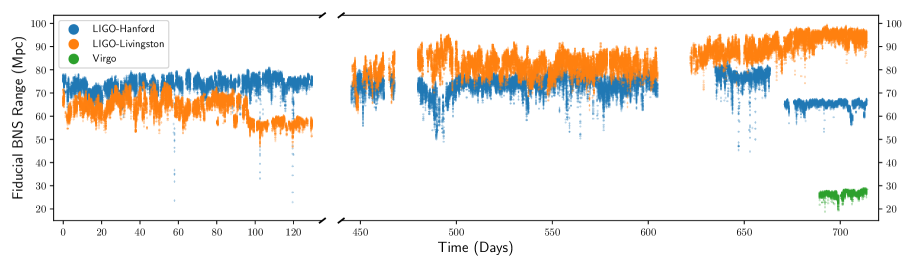
Figure 1: The sky- and orientation-averaged distance up to which each observatory can detect a 1.4-1.4 $\mathrm{M}_{\odot}$BNS merger with expected SNR equal to $8$ over the O1 and O2 observing runs. The Virgo observatory did not participate in the first observing run, but joined towards the end of the second observing run.

The first open gravitational-wave catalog (1-OGC) searched for compact-binary coalescences during O1 (Nitz et al., 2019a). We extend that analysis to cover both O1 and O2 while incorporating Virgo data for the first time. During the first observing run, only the two LIGO instruments were observing. Joint three-detector observing with the Virgo instrument began in August 2017 during the second observing run.

We make additional improvements to our search by accounting for short-time variations in the network sensitivity and power spectral density (PSD) estimates directly in our ranking of candidate events. A similar procedure for tracking PSD variations was independently developed in Venumadhav et al. (2019a, b); Zackay et al. (2019b). We produce a comprehensive catalog of candidate events from our matched-filter search which covers binary neutron star (BNS), neutron star–black hole (NSBH), and binary black hole (BBH) mergers. While not individually significant on their own, sub-threshold candidates can be correlated with gamma-ray burst candidates (Nitz et al., 2019b), high-energy neutrinos (Countryman et al., 2019), optical transients (Andreoni et al., 2018; Setzer et al., 2018), and other counterparts to uncover new, fainter sources.

In addition to our broad search, we conduct a targeted analysis to uncover fainter BBH mergers. It is possible to confidently detect binary black hole mergers which are not individually significant in the context of the wider search space by considering their consistency with the population of confidently observed binary black hole mergers. The collection of highly significant detected events constrains astrophysical rates and distribution with relatively small uncertainties (Abbott et al., 2019b). For this reason, we do not yet employ this technique for binary neutron star or neutron star–black hole populations, as their rates and mass and spin distributions are much less constrained. We improve over the BBH focused analysis introduced in Nitz et al. (2019a) by considering an explicit population prior (Dent & Veitch, 2014). This focused approach is most directly comparable to the results of (Venumadhav et al., 2019b), which considers only binary black hole mergers, rather than a broad parameter search such as employed in Abbott et al. (2019a).

We find 8 highly significant binary black hole mergers at false alarm rates less than 1 per 100 years in our full analysis along with the binary neutron star merger, GW170817. No other individually significant BNS or NSBH sources were identified. However, if the population of these sources were to be better understood, it may be possible to pick out fainter mergers from our population of candidates. When we apply a ranking to search candidates that optimizes search sensitivity for a population of BBH mergers similar to that already detected, we identify a further 6 such mergers with a probability of astrophysical origin above $50\%$. These include GW170818 and GW170729 which were reported in Abbott et al. (2019a) along with GW170121, GW170727, and GW170304 which were reported in Venumadhav et al. (2019b). We report one new marginal BBH candidate, GW151205. Our results are broadly consistent with both Venumadhav et al. (2019b) and Abbott et al. (2019a).

Table 1: Observing time in days for different instrument observing combinations. We use here the abbreviations H, L, and V for the LIGO-Hanford, LIGO-Livingston, and Virgo observatories respectively. Note that some data ($\sim\!0.5\%$) may not be analyzed due to analysis constraints. Only the indicated combination of observatories were operating for each time period, hence each is exclusive of all others.

Observing	Time(days)
H	65.4
L	50.0
V	1.7
HL	151.8
LV	2.2
HV	1.7
HLV	15.2

2 LIGO and Virgo Observing Period

We analyze the complete set of public LIGO and Virgo data (Vallisneri et al., 2015). The distribution of multi-detector analysis time and the evolution of the observatories’ sensitivities over time is shown in Table 1 and Fig. 1 respectively. To date, there has been 288 days of Advanced LIGO and Virgo observing time. Two or more instruments were observing during 171 days. There were only 15.2 days of full LIGO-Hanford, LIGO-Livingston, and Virgo joint observing. O2 was the first time that Virgo has conducted joint observing with the LIGO interferometers since initial LIGO (Abbott et al., 2016a). The Virgo instrument significantly surpassed the average BNS range during the last VSR2/3 science run ($\sim 10$ Mpc) (Abadie et al., 2012) to achieve an average of  27 Mpc during the joint observing period of O2. While the amount of triple-detector observing time is limited during the first two observing runs, the ongoing third observing run will considerably improve the availability of three-detector joint observing time. The methods demonstrated here will be applicable to future analysis of the O3 multi-detector dataset. Our analysis during triple-detector time remains sensitive to signals which appear only in two of the three detectors, as discussed below in section 3.3.

We note that there is $\sim 117$ days of single-detector observing time. In this work we do not consider the detection of gravitational-wave mergers during this time, however, methods for assigning meaningful significance to such events has been proposed (Callister et al., 2017) and will be investigated in future work. Single-detector observing time has been used in follow-up analyses where a merger could be confirmed by electromagnetic observations (Nitz et al., 2019b; Abbott et al., 2019c).

3 Search for Binary Mergers

We use a matched-filtering approach as implemented in the open source PyCBC library (Usman et al., 2016; Allen, 2005; Nitz et al., 2019c). This toolkit has been similarly employed in LIGO/Virgo collaboration and independent analyses (Abbott et al., 2019a; Nitz et al., 2019a). We extend the approach used in the 1-OGC analysis (Nitz et al., 2019a) to handle the analysis of Virgo data. We also incorporate improvements to the ranking of candidates by accounting for time variations in the power spectral density and network sensitivity.

The search procedure can be summarized as follows. The data from each detector is correlated against a set of possible merger signals. Matched filtering is used to calculate a signal-to-noise (SNR) time series for each potential signal waveform. Our analysis identifies peaks in these time series and follows up the peaks with a set of signal consistency tests. These single-detector candidates are then combined into multi-detector candidates by enforcing astrophysically consistent time delays between detectors, as well as enforcing identical component masses and spins. Finally, these candidates are ranked by the ratio of their signal and noise model likelihoods (see Sec. 3.3).

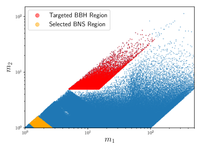
Figure 2: The component masses of templates used to search for compact binary mergers. Templates in the targeted-binary black hole region, defined by $m_{1,2}>5\,\mathrm{M}_{\odot}$, $1/3<m_{1}/m_{2}<3$, and $\mathcal{M}<60\,\mathrm{M}_{\odot}$, where $\mathcal{M}$ is the chirp mass, are colored in red (see Sec. 3.5)

. Candidates which fall in the selected BNS-like region are discussed in 4.2.

3.1 Search Space

Our analysis targets a wide range of BNS, NSBH, and BBH mergers. We perform a matched filter on the data with waveform models that span the range of desired detectable sources. Although the space of possible binary component masses and spins is continuous, we must select a discrete set of points in this space as templates to correlate against the data: we use the set of $\sim 400,000$ templates introduced in Dal Canton & Harry (2017) which has been previously used in Nitz et al. (2019a) and Abbott et al. (2019a). This bank of templates is suitable for the detection of mergers up to binary masses of several hundred solar masses, under the conditions that the dominant gravitational-wave emission mode is adequate to describe the signal and that the effects of precession caused by misalignment of the orbital and component object angular momenta can be neglected Dal Canton & Harry (2017). Neglecting precession causes a 7% (14%) loss in sensitivity to BBH (NSBH) sources with mass ratio 5 (14) when assuming an isotropic distribution of the components’ spins; the loss is negligible for mergers with comparable component masses (Harry et al., 2016). Fig. 2 shows the distribution of template detector-frame component masses. We use the spinning effective-one-body model (SEOBNRv4) for templates corresponding to mergers with (redshifted, detector frame) total mass $m_{1}+m_{2}>4\,M_{\odot}$ (Taracchini et al., 2014; Bohé et al., 2016). The TaylorF2 post-Newtonian model is used in all other cases (Sathyaprakash & Dhurandhar, 1991; Droz et al., 1999; Blanchet, 2002; Faye et al., 2012).

3.2 Single-detector Candidates

The first stage of our analysis is to identify single-detector candidates. These correspond to peaks in the SNR time series of a particular template waveform. Each is assigned a ranking statistic as we’ll discuss below. In this work, we do not explicitly conduct a search for sources which only appear in a single detector. However, a ranking of single-detector candidates forms the first stage of our analysis. For each template waveform and detector dataset we calculate a signal-to-noise time series $\rho(t)$ using matched filtering. This can be expressed using a frequency-domain convolution as

$$\rho(t)=4\Re\int_{f_{l}}^{f_{h}}{\frac{\tilde{h}^{*}(f)\tilde{s}(f)}{S_{n}(f)}e^{2\pi ift}\,df},$$ (1)

where $\tilde{h}$ is the normalized (Fourier domain) template waveform and $\tilde{s}$ is the detector data. $S_{n}$ is the noise power spectral density (PSD) of the data which is estimated using Welch’s method. The integration range extends from a template-dependent lower frequency limit $f_{l}$ (ranging from 20-30Hz in our search) to an upper cutoff $f_{h}$ given by the Nyquist frequency of the data. Peaks in the SNR time series are collected as single-detector candidates (triggers). To control the rate of single-detector candidates to be examined, our analysis pre-clusters these triggers. Only those which are amongst the loudest 100 every $\sim 1$ s within a set of predefined chirp-mass bins are kept. The binning ensures that loud triggers from a specific region (which may be caused by non-Gaussian noise artifacts) do not cause quiet signals elsewhere in parameter space to be missed.

We remove candidates where the instrument state indicates the data may be adversely affected by instrumental or environment noise artefacts as indicated by the Gravitational-Wave Open Science Center (GWOSC) (Abbott et al., 2016b, 2018; Vallisneri et al., 2015). This affects $\sim 0.5\%$ of the observation period. However, there remain classes of transient non-Gaussian noise in the LIGO data which produce triggers with large values of SNR (Nuttall et al., 2015; Abbott et al., 2016b, 2018; Cabero et al., 2019). The surviving single-detector candidates are subjected to the signal consistency tests introduced in Allen (2005) and Nitz (2018). These tests check that the accumulation of signal power as a function of frequency, and power outside the expected signal band, respectively, are consistent with an astrophysical explanation. They produce two statistic values which are $\chi^{2}$ distributed: $\chi_{r}^{2}$ and $\chi_{r,sg}^{2}$ respectively (Nitz, 2018). These are used to re-weight (Babak et al., 2013) the single-detector signal strength in two stages. This re-weighting allows candidates which well match an expected astrophysical source to be assigned a statistic value similar to their matched filter SNR, while down-weighting many classes of non-Gaussian noise transients. For all candidates we apply

$$\tilde{\rho}=\begin{cases}\rho,&\mathrm{for}\ \chi^{2}_{r}\leq 1\\ \rho\left[\frac{1}{2}\left(1+\left(\chi^{2}_{r}\right)^{3}\right)\right]^{-1/6},&\mathrm{for}\ \chi^{2}_{r}>1.\end{cases}$$ (2)

For single-detector candidates in templates with (detector-frame) total mass greater than $40\,\mathrm{M}_{\odot}$ the statistic is further re-weighted as

$$\hat{\rho}=\begin{cases}\tilde{\rho},&\mathrm{for}\ \chi^{2}_{r,sg}\leq 4\\ \tilde{\rho}(\chi^{2}_{r,sg}/4)^{-1/2},&\mathrm{for}\ \chi^{2}_{r,sg}>4.\end{cases}$$ (3)

The latter test is only applied to these short duration, higher mass signals as the test is computationally intensive and has the greatest impact for short duration signals which may be otherwise confused with some classes of transient non-Gaussian noise (Nitz, 2018; Cabero et al., 2019). Otherwise, we set $\hat{\rho}=\tilde{\rho}$.

This statistic $\hat{\rho}$ is the same used in the 1-OGC analysis (Nitz et al., 2019a) and LVC O2 catalog Abbott et al. (2019a). We further improve upon this by accounting for short-term changes in the overall PSD estimate. The issue of PSD variation was also addressed in Venumadhav et al. (2019a). Previously we modeled the PSD for each detector as a function of frequency $S_{n}(f)$, which is estimated on a 512 second timescale. We now introduce a time-dependent factor $v_{S}(t)$ which accounts for short-term O(10s) variations in sensitivity, estimated using the method described in Mozzon et al. (2020). Short-term variation in the PSD will introduce variation in $\rho$ as we use the estimated PSD $S(f)$ to calculate it. The estimated PSD over short time scales $S_{s}(f)$ can be different from a PSD estimated over a longer duration $S_{l}(f)$ if the noise is non-stationary.

To track the variation in the PSD we use the variance of the SNR. In the absence of a signal, this is given by

$$\langle\rho^{2}\rangle=\left[\int_{f_{l}}^{f_{h}}\frac{|\tilde{h}(f)|^{2}}{S_{l}(f)}\,df\right]^{-1}\int_{f_{l}}^{f_{h}}\frac{|\tilde{h}(f)|^{2}}{S_{l}(f)}\frac{S_{s}(f)}{S_{l}(f)}\,df.$$ (4)

The variance is equal to $1$ if $S_{s}(f)=S_{l}(f)$. To estimate the variance of the SNR, we first filter the detector data $\tilde{s}$ with $F(f)=\mathcal{N}|\tilde{h}(f)|/S_{l}(f)$, where $\mathcal{N}$ is a normalization constant and $|\tilde{h}(f)|$ is an approximation to the Fourier domain amplitude of CBC templates. Using Parseval’s theorem, we can then estimate the variation in the PSD at a given time $t_{0}$ as

$$v_{S}(t_{0})=\int_{t_{0}-\Delta t}^{t_{0}}|\mathcal{F}(t)*s(t)|^{2}\,dt,$$ (5)

where $\mathcal{F}(t)*s(t)$ is the convolution between the filter and the data and $\Delta t$ is chosen to match the typical time scale of non-stationarity.

After finding $v_{S}(t)$, we evaluate its correlation with the SNRs and rates of noise triggers empirically. The rate of noise triggers above a given statistic threshold is $R_{N}(>\hat{\rho}_{t})$, where the statistic $\hat{\rho}$ is (proportional to) the SNR obtained by matched filtering using the long-duration PSD $S_{l}(f)$. The noise trigger rate varies over time due to the non-stationarity of the PSD and is thus a function of the short-duration PSD variation measure. Since SNR scales as $1/\sqrt{S(f)}$, we naively expect the noise trigger rate to be a function of a ‘corrected’ SNR $\hat{\rho}/\sqrt{v_{S}}$; in practice we allow for a more general dependence which we write as

$$R_{N}(>\hat{\rho}_{t})\simeq f_{N}(\hat{\rho}_{t}v_{S}(t)^{-\kappa}).$$ (6)

Here $f_{N}$ is a fitting function for the expected noise distribution. Empirically we find, for data without strong localized non-Gaussian transients (glitches), $f_{N}(\hat{\rho})\simeq\exp(-\alpha\hat{\rho}^{2}/2)$ with $\alpha\simeq 1$.

Linearizing the PSD variation measure $v_{S}(t)$ around unity, $v_{S}(t)=1+\epsilon_{S}$, the logarithm of the trigger rate above threshold will vary as

$$\ln(R_{N}(>\hat{\rho}_{t}))\simeq\mathrm{const.}-\frac{\alpha}{2}\hat{\rho}_{t}^{2}+\alpha\kappa\hat{\rho}_{t}^{2}\epsilon_{S}$$ (7)

By determining the slope of the log-rate versus $\epsilon_{S}$ dependence for various thresholds $\hat{\rho}$ we estimate $\kappa\sim 0.33$, thus if we construct a ‘corrected’ statistic

$$\hat{\rho}\xrightarrow{}\hat{\rho}v_{S}(t)^{-0.33},$$ (8)

the rate of noise triggers above a given threshold of the corrected statistic is on average no longer affected by variation in $v_{S}(t)$.

The analysis of Venumadhav et al. (2019a) included a similar correction factor and Zackay et al. (2019b) indicates a modest improvement in sensitivity for the sources they consider. In our analysis, the greatest improvement is for sources corresponding to long-duration templates (BNS and NSBH) while there is negligible improvement for the shorter-duration BBH sources.

3.3 Multi-detector Coincident Candidates

In the previous section, we discussed how we identify single-detector candidates and assign them a ranking statistic. We now combine single-detector candidates from multiple detectors to form multi-detector candidates (Davies et al., 2020). We introduce a new ranking statistic formed from models of the relative signal and noise likelihoods for a particular candidate. This ranking statistic is based on the expected rates of signal and noise candidates, and is thus comparable across different combinations of detectors by design. We are then able to search for coincident triggers in all available combinations of detectors (for instance during HLV time, coincidences can be formed in HL, HV, LV and HLV), and then compared to one another, clustering and combining false alarm rates while maintaining near-optimal sensitivity.

Our signal model is composed of two parts. First, the overall network sensitivity of the analysis at the time of the candidate. Assuming a spatially homogeneous distribution of sources, the signal rate is directly proportional to the sensitive volume. We approximate this factor using the instantaneous range of the least sensitive instrument contributing to the multi-detector candidate for a given template labelled by $i$, $\sigma_{{\rm min},i}$, relative to a representative range over the analysis, which is defined by the median network sensitivity in the HL detector network, $\overline{\sigma}_{HL,i}$, for that template. Note that the detectors which contribute to the candidate are not necessarily all of the available detectors at that time. The second part is the probability, given an isotropic and volumetric population of sources, that an astrophysical signal would be observed to have a particular set of parameters defined by $\vec{\theta}$, including time delays, relative amplitudes, and relative phases between the network of observatories. This probability distribution $p(\vec{\theta}|S)$ is calculated by a Monte Carlo method similarly to Nitz et al. (2017). For this work we have extended this technique to three detectors for the first time. Combined, our model for the density of signals recovered with network parameters $\vec{\theta}$ in a combination of instruments characterized by $\sigma_{min,i}$ can be expressed as

$$R_{S,i}(\vec{\theta})=\left(\frac{\sigma_{{\rm min},i}}{\overline{\sigma}_{HL,i}}\right)^{3}p(\vec{\theta}|S).$$ (9)

The noise model is calculated in the same manner as in  Nitz et al. (2017). We treat the noise from each detector as being independent and fit our single-detector ranking statistic to an exponential slope. This fit is performed separately for each template. The fit parameters (such as the slope and overall amplitude of the exponential) are initially noisy due to low number statistics, so they are smoothed over the template space using a three-dimensional Gaussian kernel in the template duration, effective spin $\chi_{\mathrm{eff}}$, and symmetric mass ratio $\eta$ parameters. The rate density of noise events in the $i^{\textrm{th}}$ template with contributing detectors labelled by $n$ and single-detector rankings $\{\tilde{\rho}_{n}\}$ can be summarized as

$$R_{N,i}(\{\tilde{\rho}_{n}\})=A_{\{n\}}\prod_{n}{r_{n,i}e^{-\alpha_{n,i}\tilde{\rho}_{n}}},$$ (10)

where $r_{n,i}$ and $\alpha_{i}$ are the overall amplitude and slope of the exponential noise rate model respectively. The prefactor $A_{\{n\}}$ is the time window for which coincidences can be formed, which depends on the combination of detectors $\{n\}$ being considered. The three-detector coincidence rate is vastly reduced compared to the two-detector rate; in a representative stretch of O2 data, the HLV coincidence rate is found to be around a factor of $10^{4}$ lower than that in HL coincidences. Details of both the signal and noise model calculations will be provided in Davies et al. (2020).

The ranking statistic for a given candidate in template $i$ is the log of the ratio of these two rate densities:

$$\tilde{\Lambda}=\log(R_{S,i}/R_{N,i})+\mathrm{const.},$$ (11)

where we drop the dependencies on $\vec{\theta}$ and $\{\tilde{\rho}_{n}\}$ for simplicity of notation. Typically, one signal event (or loud noise event) in the gravitational-wave data stream may give rise to a large number of correlated candidate multi-detector events within a short time, in different templates and with different combinations of detectors $\{n\}$. To calculate the significance of such a ‘cluster’ of events, we will approximate their arrival as a Poisson process: in order to do this, we keep the event from each cluster with highest $\tilde{\Lambda}$ — typically the highest-ranked event within a 10 s time window — and discard the rest.

Comparing this new statistic to the one employed for the 1-OGC analysis (Nitz et al., 2019a) using a simulated population of mergers, we find an average $8\%$ increase in the detectable volume during the O1 period at a fixed false alarm rate of 1 per 100 years. This population is isotropically distributed in sky location and orientation, while the mass distribution is scaled to ensure a constant rate of signals above a fixed SNR across the log-component-mass search space in Fig. 2. In addition to this improved sensitivity for events where H1 and L1 contribute, this search will also benefit by analyzing times where Virgo and only one LIGO detector are operating (as in Table 1), and also by improved sensitivity in times when all three detectors are operating, due to the ability to form 3-detector events. Such sensitivity improvements are detailed in Davies et al. (2020).

3.4 Statistical Significance

In the previous section we introduce the ranking statistic used in our analysis. We empirically measure the statistical significance of a particular value of our ranking statistic by comparing it to a set of false (noise) candidate events produced in numerous fictitious analyses. Each such analysis is generated by time-shifting the data from one detector by an amount greater than is astrophysically allowed by light travel time considerations Babak et al. (2013); Usman et al. (2016). Otherwise, each time-shifted analysis is treated in the identical manner as the search itself. By repeating this procedure, upwards of $10^{4}$ years’ worth of false alarms can be produced from just a few days of data. By construction, the results of these analyses cannot contain true multi-detector astrophysical candidates, but may contain coincidences between astrophysical sources and instrumental noise. We use a hierarchical procedure as in Abbott et al. (2016c) and Nitz et al. (2019a) to minimize the impact of astrophysical contamination while retaining an unbiased rate of false alarms (Capano et al., 2017): a candidate with large $\tilde{\Lambda}$ is removed from the estimation of background for less significant candidates.

This method has been employed to detect significant events in numerous analyses (Nitz et al., 2019a; Abbott et al., 2019a; Venumadhav et al., 2019b; Abadie et al., 2012; Abbott et al., 2009). The validity of the resulting background estimate follows from an assumption that the times of occurrence of noise events are statistically independent between different detectors; see Was et al. (2010); Capano et al. (2017) for further discussion of empirical background estimation and the time shift method. This is a reasonable assumption for detectors separated by thousands of kilometres (Abbott et al., 2016b). The time shift method has the advantage that no other assumptions about the noise need be accurate: the populations and morphology of noise artefacts need not be uncorrelated or different between detectors, only the times at which they occur. In fact the LIGO and Virgo instruments share common components and environmental coupling mechanisms which may produce similar classes of non-Gaussian artefacts.

Table 2: Candidate events in the full search of O1 and O2 data. Candidates are sorted by FAR evaluated for the entire bank of templates. Note that ranking statistic and false alarm rate may not have a strictly monotonic relationship due to varying data quality between sub-analyses. The mass and spin parameters listed are associated with the template waveform yielding the highest ranked multi-detector event for each candidate, and may differ significantly from full Bayesian parameter estimates. Masses are quoted in detector frame, and are thus larger than source frame masses by a factor $(1+z)$, where $z$ is the source redshift.

Date designation	GPS time	FAR-1 (y)	Detectors	$\tilde{\Lambda}$	$\rho_{H}$	$\rho_{L}$	$\rho_{V}$	$m_{1}^{t}$	$m_{2}^{t}$	$\chi_{\mathrm{eff}}^{t}$
170817+12:41:04UTCx	1187008882.45	$>10000$	HL	180.46	18.6	24.3	-	1.5	1.3	-0.00
150914+09:50:45UTCxyz	1126259462.43	$>10000$	HL	93.82	19.7	13.4	-	44.2	32.2	0.09
170104+10:11:58UTCxz	1167559936.60	$>10000$	HL	35.54	9.0	9.6	-	47.9	16.0	0.03
170823+13:13:58UTCxz	1187529256.52	$>10000$	HL	55.04	6.3	9.2	-	68.9	47.2	0.23
170814+10:30:43UTCxz	1186741861.54	$>10000$	HL	52.85	9.0	13.0	-	58.7	23.3	0.53
151226+03:38:53UTCxyz	1135136350.65	$>10000$	HL	42.90	10.7	7.4	-	14.8	8.5	0.24
170809+08:28:21UTCxz	1186302519.76	9400	HL	40.59	6.6	10.7	-	36.0	33.7	0.07
170608+02:01:16UTCx	1180922494.49	$>910$	HL	51.01	12.5	8.7	-	16.8	6.1	0.31
151012+09:54:43UTCxyz	1128678900.45	220	HL	20.18	7.0	6.7	-	30.8	12.9	-0.05
170729+18:56:29UTCxz	1185389807.33	6.4	HL	15.33	7.4	6.7	-	106.5	49.7	0.59
170121+21:25:36UTCz	1169069154.58	1.3	HL	15.76	5.1	8.7	-	40.4	13.6	-0.98
170727+01:04:30UTCz	1185152688.03	.53	HL	13.75	4.5	6.9	-	65.2	26.5	-0.35
170818+02:25:09UTCx	1187058327.09	.22	HL	13.29	4.4	9.4	-	53.7	27.4	0.07
170722+08:45:14UTC	1184748332.91	.11	HL	12.19	5.0	6.4	-	248.1	7.1	0.99
170321+03:13:21UTC	1174101219.23	.1	HL	12.22	6.5	6.4	-	11.0	1.3	-0.89
170310+09:30:52UTC	1173173470.77	.07	HL	12.15	6.1	6.2	-	2.1	1.1	-0.20
170809+03:55:52UTC	1186286170.08	.07	LV	7.34	-	7.0	5.1	6.2	1.2	0.60
170819+07:30:53UTC	1187163071.23	.05	HV	11.35	6.3	-	6.7	135.2	2.5	0.85
170618+20:00:39UTC	1181851257.72	.05	HL	11.49	5.2	6.7	-	2.9	2.1	0.30
170416+18:38:48UTC	1176403146.15	.04	HL	11.21	5.1	6.9	-	7.8	1.1	-0.47
170331+07:08:18UTC	1174979316.31	.04	HL	11.03	5.2	7.0	-	3.9	1.1	-0.34
151216+18:49:30UTC	1134326987.60	.04	HL	11.54	6.1	6.0	-	13.9	5.0	-0.41
170306+04:45:50UTC	1172810768.08	.04	HL	11.47	4.8	7.3	-	26.4	1.8	0.23
151227+16:52:22UTC	1135270359.27	.04	HL	11.75	7.3	4.6	-	154.5	4.9	1.00
170126+23:56:22UTC	1169510200.17	.04	HL	11.61	6.4	5.7	-	4.9	1.3	0.79
151202+01:18:13UTC	1133054310.55	.03	HL	11.48	6.5	5.7	-	40.4	1.8	-0.26
170208+20:23:00UTC	1170620598.15	.03	HL	11.12	6.8	5.4	-	6.9	1.0	0.09
170327+17:07:35UTC	1174669673.72	.03	HL	10.65	6.0	6.2	-	40.1	1.0	0.97
170823+13:40:55UTC	1187530873.86	.03	LV	9.30	-	8.0	5.8	117.9	1.3	0.98
150928+10:49:00UTC	1127472557.93	.03	HL	11.28	6.0	6.3	-	2.5	1.0	-0.70

^xAlso identified in GWTC-1 (Abbott et al., 2019a), ^y1-OGC (Nitz et al., 2019a), or ^zVenumadhav et al. (2019a, b)

3.5 Targeting Binary Black Hole Mergers

Given a population of individually significant BBH mergers, it is possible to incorporate knowledge about the overall distribution and rate of sources to identify weaker candidates. A similar approach was employed in Nitz et al. (2019a) and is the basis of astrophysical significance statements in Abbott et al. (2019a). In this catalog we improve over the strategy of Nitz et al. (2019a) which considered an excessively conservative parameter space for BBH and did not use an explicit model of the distribution of signals and noise within that space. In addition, we restrict to sources which are consistent with our signal models by imposing a threshold on our primary signal consistency test to reject any single-detector candidate with $\chi_{r}>2.0$. Simulated signals within our target population, and the individual highly significant candidates previously detected are consistent with this choice. (The full, non-BBH-specific analysis allows a much greater deviation from our signal models before rejection of a candidate.)

As a first step in obtaining the targeted BBH results we restrict the analysis to a sub-space of the full search, illustrated in Fig. 2. Rather than applying this constraint after obtaining the set of ‘clustered’ candidates via selecting the highest ranked event within $10$ s windows, as in Nitz et al. (2019a), here we apply the constraint to candidates prior to the clustering step. This allows us to choose a less extensive BBH region containing fewer templates than employed in Nitz et al. (2019a) without loss of sensitivity. (The previous method used a wider BBH template set to allow for the possibility that a signal inside the intended target region is recovered only by a template lying outside that region, due to clustering.) Our BBH region is specified by $m_{1,2}>5\,\mathrm{M}_{\odot}$, $1/3<m_{1}/m_{2}<3$, and $\mathcal{M}<60\,\mathrm{M}_{\odot}$. The upper boundary is consistent with the redshifted detector-frame masses that would be obtained by the observed highest-mass sources near detection threshold.

Applying a prior over the intrinsic parameters of the distribution of detectable sources was proposed in Dent & Veitch (2014) and tested in Nitz et al. (2017). In this work, we impose an explicit detection prior that is flat over chirp mass. As seen in Fig. 2, the distribution of templates is highly non-uniform. The BBH region of template is placed first using a stochastic algorithm (Dal Canton & Harry, 2017; Ajith et al., 2014), where density of templates directly correlates to density of effectively independent noise events. The template density over $\mathcal{M}$ scales as $\mathcal{M}^{-11/3}$, which we verify empirically for our bank. Our detection statistic aims to follow the relative rate density of signal versus noise events at fixed SNR, and we make the simple choice of assuming a signal density flat over $\mathcal{M}$: thus the ranking statistic receives an extra term describing the ratio of signal to noise densities over component masses:

$$\tilde{\Lambda}{}_{\rm BBH}=\tilde{\Lambda}{}+\frac{11}{3}\ln\left(\frac{\mathcal{M}}{\mathcal{M}_{f}}\right),$$ (12)

where $\mathcal{M}_{f}=20\,\mathrm{M}_{\odot}$ is a fiducial reference mass scale. Roughly, any given lower-mass template is less likely to detect a signal than a higher-mass template given that templates are much sparser at high masses.

Our choice of BBH region and detection prior has a similar effect as the highly constrained search space and multiple chirp mass bins used in Venumadhav et al. (2019b) but avoids the multiple boundary effects present there and provides a more clearly implemented and astrophysically motivated prior distribution. Furthermore, our method provides a path forward to more accurate assessment of lower-SNR candidates as our understanding of the overall population evolves.

To estimate the probability $p_{\mathrm{astro}}$ that a given candidate is astrophysical in origin we combine the background of this targeted BBH analysis with the estimated distribution of observations. We improve upon the analysis in Nitz et al. (2019a) which employed an analytic model of the signal distribution and a fixed conservative rate of mergers by using the mixture model method developed in Farr et al. (2015) and similar to that employed in Abbott et al. (2019a). This method requires the distribution of noise and signals over our ranking statistic, which we take from our time-slide background estimates and a population of simulated signals respectively.

Using a simulated set of mergers that is isotropically distributed in orientation and uniformly distributed over mass to cover the targeted BBH region, we find that the targeted BBH analysis recovers a factor $1.5$–$1.6$ more sources at a fixed false alarm rate of 1 per 100 years than the full parameter space analysis. The majority of this change in sensitivity is attributed to the inclusion of only background events consistent with BBH mergers. The choice of ranking statistic to optimize sensitivity to a target BBH signal population has a smaller effect.

Table 3: Candidates from the targeted binary black hole sub-region sorted by the probability they are astrophysical in origin. The source-frame masses, $\chi_{\mathrm{eff}}$, and luminosity distance $D_{L}$ are estimated with Bayesian parameter inference (see Sec. 4.1) and are given with $90\%$ credible intervals.

Date designation	GPS time	$p_{\mathrm{astro}}$	FAR-1 (y)	Det.	$\tilde{\Lambda}_{\rm BBH}$	$\rho_{H}$	$\rho_{L}$	$\rho_{V}$	$m^{\mathrm{src}}_{1}$	$m^{\mathrm{src}}_{2}$	$\chi_{\mathrm{eff}}$	$D_{L}$ (Mpc)
150914+09:50:45UTCxyz	1126259462.43	$>0.999$	$>10000$	HL	111.71	19.7	13.4	-	$35.4^{+5.3}_{-3.2}$	$29.8^{+3.1}_{-4.7}$	$-0.04^{+0.11}_{-0.13}$	$470^{+140}_{-190}$
170814+10:30:43UTCxz	1186741861.53	$>0.999$	$>10000$	HL	61.58	9.3	13.8	-	$30.4^{+5.6}_{-2.7}$	$25.8^{+2.6}_{-4}$	$0.08^{+0.12}_{-0.12}$	$580^{+130}_{-190}$
170823+13:13:58UTCxz	1187529256.52	$>0.999$	$>10000$	HL	59.43	6.3	9.2	-	$40^{+11.7}_{-7.1}$	$28.8^{+6.8}_{-7.9}$	$0.05^{+0.21}_{-0.22}$	$1750^{+850}_{-820}$
170104+10:11:58UTCxz	1167559936.60	$>0.999$	$>10000$	HL	47.32	9.1	9.9	-	$31.6^{+7.8}_{-6.3}$	$19.2^{+5}_{-4.1}$	$-0.08^{+0.16}_{-0.18}$	$920^{+420}_{-400}$
151226+03:38:53UTCxyz	1135136350.65	$>0.999$	$>10000$	HL	40.58	10.7	7.4	-	$13.9^{+7.9}_{-3.3}$	$7.6^{+2.2}_{-2.3}$	$0.209^{+0.177}_{-0.077}$	$460^{+160}_{-180}$
151012+09:54:43UTCxyz	1128678900.45	$>0.999$	$>10000$	HL	20.25	7.0	6.7	-	$22.4^{+13.4}_{-4.8}$	$13.8^{+3.7}_{-4.8}$	$-0.00^{+0.25}_{-0.16}$	$990^{+470}_{-460}$
170809+08:28:21UTCxz	1186302519.76	$>0.999$	8300	HL	43.34	6.6	10.7	-	$35.2^{+9.5}_{-5.9}$	$23.9^{+5.1}_{-5.3}$	$0.06^{+0.18}_{-0.16}$	$980^{+310}_{-390}$
170729+18:56:29UTCxz	1185389807.33	$>0.999$	4000	HL	19.16	7.5	7.1	-	$55^{+18}_{-13}$	$32^{+13}_{-10}$	$0.31^{+0.22}_{-0.29}$	$2300^{+1600}_{-1300}$
170608+02:01:16UTCx	1180922494.49	$>0.999$	$>910$	HL	55.12	12.5	8.7	-	$11.6^{+6.7}_{-2.1}$	$7.4^{+1.6}_{-2.3}$	$0.088^{+0.213}_{-0.073}$	$310^{+130}_{-110}$
170121+21:25:36UTCz	1169069154.58	$>0.999$	2104	HL	23.86	5.1	8.9	-	$33^{+9.2}_{-5.3}$	$25.7^{+5.3}_{-6.1}$	$-0.17^{+0.24}_{-0.26}$	$1150^{+950}_{-650}$
170818+02:25:09UTCx	1187058327.09	$>0.999$	5.14	HL	21.42	4.4	9.4	-	$36^{+8.2}_{-5.3}$	$26.2^{+4.8}_{-5.7}$	$-0.11^{+0.20}_{-0.23}$	$980^{+430}_{-340}$
170727+01:04:30UTCz	1185152688.03	0.994	180	HL	15.84	4.5	6.9	-	$41.6^{+12.8}_{-7.9}$	$30.4^{+7.9}_{-8.2}$	$-0.05^{+0.25}_{-0.30}$	$2200^{+1500}_{-1100}$
170304+16:37:53UTCz	1172680691.37	0.70	2.5	HL	11.61	4.6	7.1	-	$44.9^{+17.6}_{-9.4}$	$31.8^{+9.5}_{-11.6}$	$0.11^{+0.29}_{-0.27}$	$2300^{+1600}_{-1200}$
151205+19:55:25UTC	1133380542.42	0.53	.61	HL	10.97	5.8	4.8	-	$67^{+28}_{-17}$	$42^{+16}_{-19}$	$0.14^{+0.40}_{-0.38}$	$3000^{+2400}_{-1600}$
151217+03:47:49UTC	1134359286.35	0.26	.15	HL	9.61	6.7	5.6	-	$46^{+13}_{-26}$	$8.2^{+5.1}_{-1.7}$	$0.70^{+0.15}_{-0.50}$	$1000^{+660}_{-440}$
170201+11:03:12UTC	1169982210.74	0.24	.16	HL	9.26	6.0	5.6	-	$48^{+13}_{-23}$	$13.1^{+8.6}_{-3.7}$	$0.44^{+0.28}_{-0.54}$	$1530^{+1360}_{-770}$
170425+05:53:34UTCz	1177134832.19	0.21	.2	HL	9.42	5.1	5.8	-	$45^{+21}_{-11}$	$30^{+11}_{-11}$	$-0.06^{+0.28}_{-0.32}$	$2600^{+2000}_{-1300}$
151216+09:24:16UTCyz	1134293073.19	0.18	.1	HL	9.25	5.9	5.5	-	$41^{+15}_{-17}$	$14.4^{+7}_{-6.3}$	$0.51^{+0.21}_{-0.57}$	$1620^{+1140}_{-910}$
170202+13:56:57UTCz	1170079035.73	0.13	.06	HL	8.37	5.0	6.6	-	$33^{+17}_{-11}$	$13.8^{+7}_{-4.8}$	$-0.06^{+0.27}_{-0.32}$	$1220^{+980}_{-640}$
170104+21:58:40UTC	1167602338.72	0.12	.03	HL	8.80	5.6	5.4	-	$98^{+49}_{-40}$	$44^{+30}_{-33}$	$0.25^{+0.50}_{-0.49}$	$4600^{+4300}_{-3100}$
170220+11:36:24UTC	1171625802.53	0.10	.05	HL	8.43	4.4	5.2	-	$69^{+37}_{-25}$	$31^{+22}_{-14}$	$0.28^{+0.33}_{-0.37}$	$3600^{+3700}_{-2100}$
170123+20:16:42UTC	1169237820.55	0.08	.04	HL	7.97	5.0	5.3	-	$44^{+23}_{-12}$	$28^{+13}_{-13}$	$-0.12^{+0.31}_{-0.35}$	$2800^{+2800}_{-1600}$
151011+19:27:49UTC	1128626886.61	0.08	.12	HL	8.45	4.9	6.6	-	$51^{+18}_{-12}$	$31^{+12}_{-12}$	$0.09^{+0.29}_{-0.27}$	$1560^{+1090}_{-740}$
151216+18:49:30UTC	1134326987.60	0.07	.03	HL	8.14	6.1	6.0	-	$19.7^{+6.4}_{-7.4}$	$3.25^{+1.32}_{-0.58}$	$-0.03^{+0.24}_{-0.49}$	$500^{+280}_{-250}$
170721+05:55:13UTC	1184651731.37	0.06	.04	HL	7.76	6.6	5.1	-	$31.7^{+9.3}_{-6.1}$	$21.4^{+5.3}_{-5.6}$	$-0.06^{+0.25}_{-0.29}$	$1160^{+750}_{-520}$
170403+23:06:11UTCz	1175295989.23	0.03	.07	HL	7.26	5.2	5.2	-	$53^{+23}_{-13}$	$35^{+13}_{-15}$	$-0.20^{+0.35}_{-0.37}$	$2500^{+2100}_{-1300}$
170629+04:13:55UTC	1182744853.11	0.02	.06	HL	6.72	6.6	4.8	-	$49^{+20}_{-30}$	$7.3^{+4.6}_{-2.6}$	$0.73^{+0.15}_{-0.98}$	$1880^{+1450}_{-940}$
170620+01:14:02UTC	1181956460.10	0.02	.04	HL	6.18	5.7	5.1	-	$29.4^{+13.2}_{-6.8}$	$17.9^{+5.4}_{-5.5}$	$0.05^{+0.25}_{-0.25}$	$1710^{+1300}_{-850}$
170801+23:28:19UTC	1185665317.35	-	.04	LV	8.59	-	6.9	4.3	$23.9^{+12.6}_{-6.6}$	$12.4^{+4.7}_{-4}$	$-0.09^{+0.25}_{-0.24}$	$1070^{+920}_{-580}$
170818+09:34:45UTC	1187084103.28	-	.04	HV	8.40	6.5	-	4.4	$55^{+59}_{-28}$	$23^{+43}_{-15}$	$0.06^{+0.48}_{-0.45}$	$3100^{+1700}_{-1900}$

^xAlso identified in GWTC-1 (Abbott et al., 2019a), ^y1-OGC (Nitz et al., 2019a), or ^zVenumadhav et al. (2019a, b)

4 Observational Results

We present compact binary merger candidates from the complete set of public LIGO and Virgo data spanning the observing runs from 2015-2017. This comprises roughly 171 days of multi-detector observing time which we divide into 31 sub-analyses. Except as noted, each analysis contains $\sim 5$ days of observing time which allows for estimation of the false alarm rate to $<$ 1 per 10,000 years. This interval allows us to track changes in the detector configuration which may result in time-changing detector quality. All data was retrieved from GWOSC Vallisneri et al. (2015), and we have used the most up-to-date version of bulk data released. We note that an exceptional data release was produced by GWOSC which contains background data relating to GW170608. We have analyzed this data release separately to preserve consistent data quality.

The top candidates sorted by FAR from the complete analysis are given in Table 2. All of the most significant candidates were observed by LIGO-Hanford and LIGO-Livingston which are the two most sensitive detectors in the network and contribute the bulk of the observing time. There are 8 BBH and 1 BNS candidates at a FAR less than 1 per 100 years. These sources are confidently detected in the full analysis without optimizing the search for any specific population of sources. The most significant following candidates correspond to GW170729, GW170121, GW170727 and GW170818 respectively. A similar PyCBC-based analysis was performed in Abbott et al. (2019a) but used a higher single-detector SNR threshold than employed in our analysis ($\rho>5.5$ vs 4.0); as the latter three events were found with $\rho<=5.1$ in the LIGO-Hanford detector, we would not expect this earlier analysis to identify them.

Table 4: Candidate events with template parameters consistent with BNS mergers sorted by ranking statistic $\tilde{\Lambda}$. The chirp mass $\mathcal{M}$ of the candidate’s associated template waveform is given in the detector frame. All candidates here were found by the LIGO-Hanford and LIGO-Livingston observatories. The table lists the false alarm rate for each candidate in the context of the full search (FAR_FULL) or just the selected BNS region (FAR_BNS).

Date Designation	GPS Time	$\tilde{\Lambda}$	FAR${}_{FULL}^{-1}$ (y)	FAR${}_{BNS}^{-1}$ (y)	$\rho_{H}$	$\rho_{L}$	$\mathcal{M}$
170817+12:41:04UTC	1187008882.45	180.46	$>10000$	$>10000$	18.6	24.3	1.20
161217+02:44:33UTC	1165977890.44	10.81	.01	.27	6.2	6.0	1.15
151214+21:03:35UTC	1134162232.89	9.26	.003	.12	6.0	5.7	1.06
151105+20:34:28UTC	1130790885.49	8.97	.002	.03	6.0	6.3	1.29
160103+02:29:54UTC	1135823411.78	8.41	.002	.04	5.3	6.5	1.16
170204+00:34:28UTC	1170203686.48	8.40	.002	.06	5.1	6.4	1.25
170819+11:06:26UTC	1187176004.83	8.37	.004	.12	6.2	6.0	1.06
170213+21:45:15UTC	1171057533.29	8.35	.002	.06	7.4	6.1	1.15
151112+05:48:49UTC	1131342546.36	8.11	.0008	.01	5.7	6.4	1.35
150930+12:45:03UTC	1127652320.31	8.10	.001	.04	6.0	5.8	1.15

4.1 Binary Black Holes

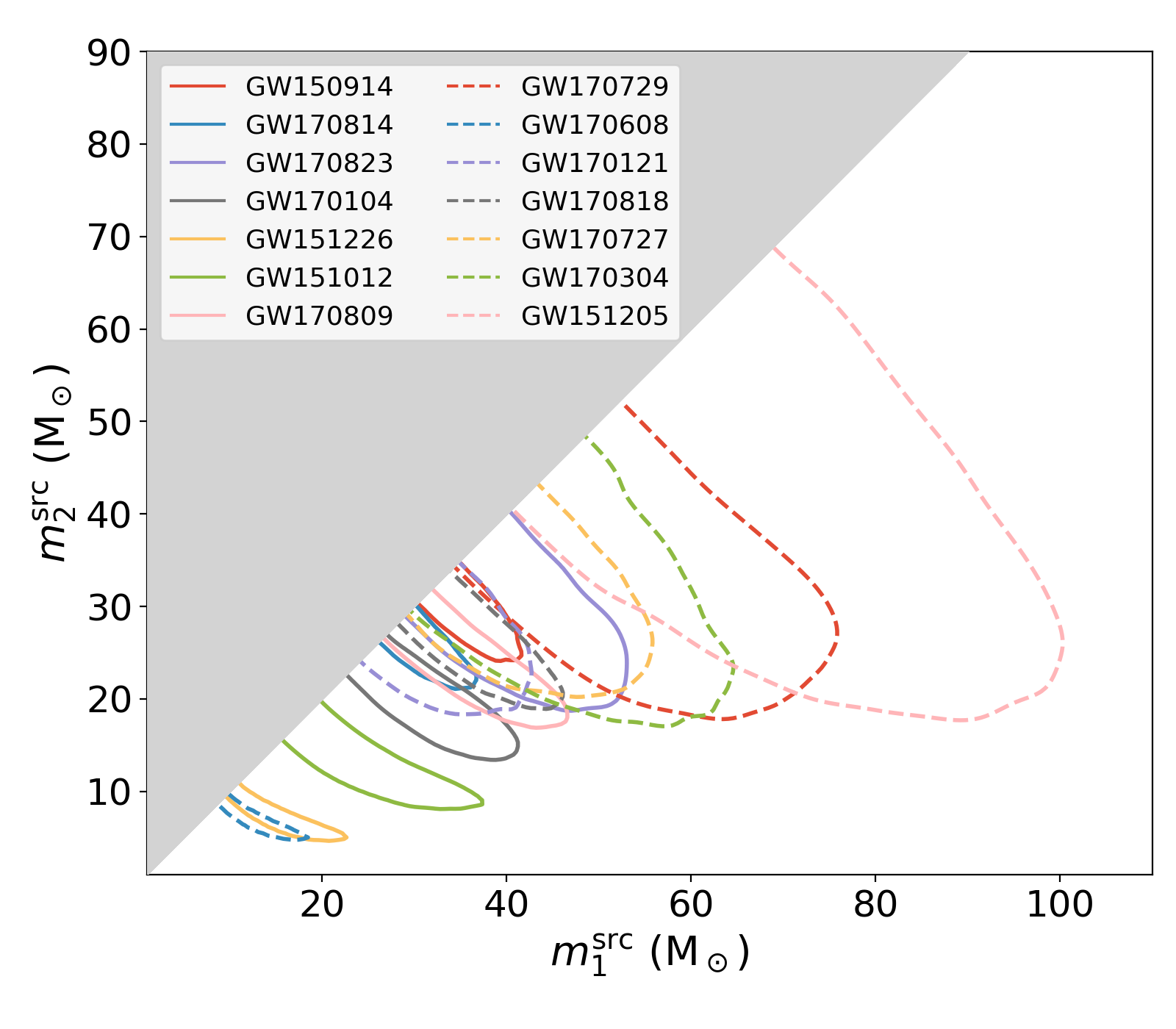
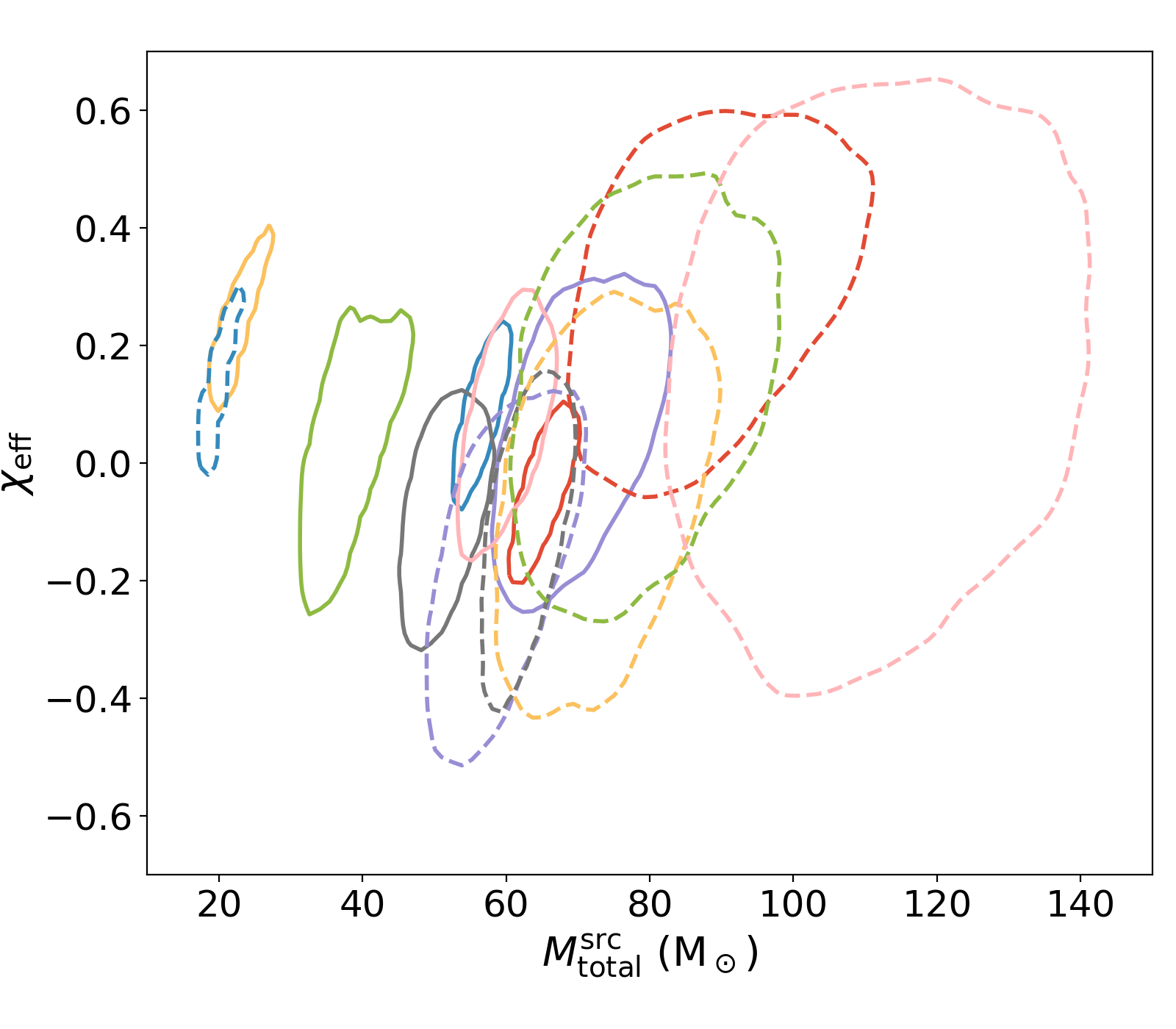
Figure 3: Marginalized $90\%$ credible region for all binary black hole candidates with $p_{\mathrm{astro}}\geq 0.5$ in source-frame component masses (left) along with source-frame total mass and effective spin (right). GW170121, GW170304 and GW170727 which were previously reported in Venumadhav et al. (2019b) are broadly consistent with the existing population of observed BBH mergers. GW151205, a new BBH candidate with $p_{\mathrm{astro}}\sim 0.53$, is likely the most massive merger reported to date if astrophysical.

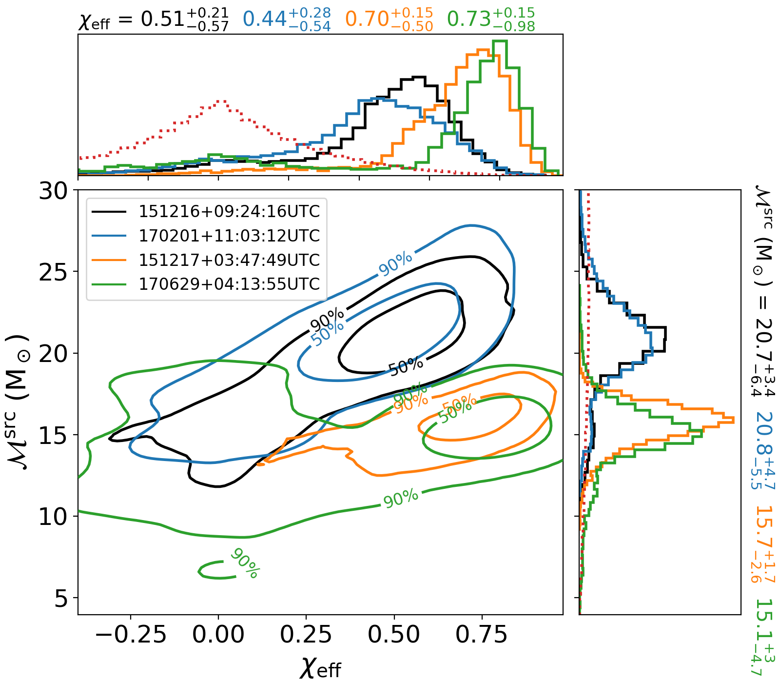
Figure 4: Comparison of marginalized $\chi_{\mathrm{eff}}$ and source-frame chirp mass $\mathcal{M}^{\rm src}$ posteriors between 151216+09:24:16UTC, 170201+11:03:12UTC, 151217+03:47:49UTC, and 170629+04:13:55UTC. The marginalized prior on each parameter is shown by the dotted red lines. Contrary to Zackay et al. (2019a), we find that 151216+09:24:16UTC has support at zero effective spin. The candidate bears striking resemblance to 170201+11:03:12UTC, and, to a lesser extent, 151217+03:47:49UTC and 170629+04:13:55UTC. All four have $\chi_{\mathrm{eff}}$ posteriors that diverge strongly from the prior (with peaks between $\sim 0.5$ and $\sim 0.7$) and similar chirp masses, which distinguishes them from the other BBH candidates in Table 3. This may indicate a new population of binary black holes, or a common noise feature. If the former, ongoing and future observing runs should yield more candidates with similar properties and larger astrophysical significance.

Using the targeted BBH analysis introduced in Sec. 3.5 we report results for BBH mergers consistent with the existing set of highly significant merger events in Table 3. The probability that a candidate is astrophysical in origin, $p_{\mathrm{astro}}$, is calculated for the most significant candidates. Our analysis identifies 14 BBH candidates with $p_{\mathrm{astro}}>50\%$, meeting the standard detection criteria introduced in Abbott et al. (2019a) and similarly followed in Venumadhav et al. (2019b). Our results are broadly consistent with the union of those two analyses as our candidate list includes all previously claimed BBH detections. We confirm the observation of GW170121, GW170304, and GW170727 reported in Venumadhav et al. (2019a) as significant. We also report the marginal detection of GW151205.

Several marginal events reported in Venumadhav et al. (2019b, a) are found as top candidates, but do not meet our detection threshold based on estimated probability of astrophysical origin. Numerous differences between these two analyses — including template bank placement, treatment of data, choice of signal consistency test, and method for assigning astrophysical significance — may be the cause of reported differences. The consistency of results for less marginal candidates indicates that differences in analysis sensitivity are likely marginal. Cross comparison with a common set of simulated signals would be required for a more precise assessment.

Future analyses incorporating more sophisticated treatment of the source distribution may yield different results for the probability of astrophysical origin for some sub-threshold candidates. For example 151216+09:24:16UTC, which was first identified in Nitz et al. (2019a) and is now assigned a $p_{\mathrm{astro}}\sim 0.2$, could obtain a higher probability of being astrophysical under a model with a distribution of detected mergers peaked close to its apparent component masses, rather than uniform over $\mathcal{M}$ as taken here. In any case the astrophysical probability we assign assumes that the candidate event, if astrophysical, is drawn from an existing population. The prior applied here to the population distribution over component masses could be extended to the distribution over component-object spins. (Here, we implicitly apply a prior over spins which mirrors the density of templates, which is not far from uniform over $\chi_{\mathrm{eff}}$.) As 151216+09:24:16UTC may have high component spins, if the set of highly significant observations does not include any comparable systems its probability of astrophysical origin could be arbitrarily small, depending on a choice of prior distribution over spins.

We infer the properties of our BBH candidates using Bayesian parameter inference implemented by the PyCBC library (Biwer et al., 2019). We use the IMRPhenomPv2 model which describes the dominant gravitational-wave mode of the inspiral-merger-ringdown of precessing non-eccentric binaries (Schmidt et al., 2015; Hannam et al., 2014). For each candidate, we use a prior isotropic in sky location and binary orientation. As in Abbott et al. (2019a), our prior on each component object’s spin is uniform in magnitude and isotropic in orientation.

Since many of the candidates are at large ($>1\,$Gpc) distances, we assume a prior which is uniform in comoving volume, and a prior uniform in source-frame component mass. We use standard $\Lambda$CDM cosmology (Ade et al., 2015) to relate the comoving volume to luminosity distance, and to redshift the masses to the detectors’ frame. This choice of prior differs from previous analyses (Abbott et al., 2019a; Venumadhav et al., 2019b, a), which used a prior uniform in volume (ignoring cosmological effects) and detector-frame masses. A prior uniform in co-moving volume assigns lower weight to large luminosity distances than a prior uniform in volume. Consequently, the luminosity distances we obtain for some candidates is slightly lower than previously reported values (e.g., we obtain $D_{L}=2300^{+1600}_{-1200}\,$Mpc for GW170729, whereas Abbott et al. (2019a) obtained $D_{L}=2840^{+1400}_{-1360}\,$Mpc).

The marginalized parameter estimates of the component masses, effective spin, and luminosity distance for the top 30 BBH candidates are given in Table 3. Plots of the marginalized posteriors for the BBH candidates with $p_{\mathrm{astro}}\geq 0.5$ is show in Fig. 3. For candidates previously reported by the LVC, our results broadly agree with existing parameter estimates (Abbott et al., 2019a; De et al., 2018). Similarly, we find no clear evidence for precession in our candidates. Venumadhav et al. (2019b) and  Zackay et al. (2019a) reported marginal high-mass BBH candidates, in particular 170403+23:06:11UTC with $\chi_{\mathrm{eff}}=-0.7^{+0.5}_{-0.3}$ and 151216+09:24:16UTC with $\chi_{\mathrm{eff}}=0.8^{+.15}_{-.21}$, which excludes $\chi_{\mathrm{eff}}\sim 0$. In addition to assigning these candidates lower astrophysical significance, we find that $\chi_{\mathrm{eff}}\sim 0$ is excluded for neither candidate. For 151216+09:24:16UTC, we find several points in the posterior around $\chi_{\mathrm{eff}}\sim 0$ with likelihood values similar to that around $\chi_{\mathrm{eff}}\sim 0.5$. This indicates that the discrepancy in $\chi_{\mathrm{eff}}$ between our analysis and that of Venumadhav et al. (2019b) cannot be entirely explained by differences in prior choice; the difference may be due to differing analysis methods.

We find three other events with $p_{\mathrm{astro}}<0.3$ that have $\chi_{\mathrm{eff}}$ and masses similar to that of 151216+09:24:16UTC. These are illustrated in Fig. 4. The four events differ from the other events listed in Table 3 in that the posterior distribution of $\chi_{\mathrm{eff}}$ strongly deviates from the prior, with the peak in the posterior between $\chi_{\mathrm{eff}}\sim 0.5$ and $\sim 0.7$. All four events also have similar chirp masses. If these events are from a new population of binary black holes, then ongoing and future observing runs should yield candidates with similar properties at high astrophysical significance. Alternatively, they may indicate a common noise feature selected by our analysis.

GW151205, a BBH merger with $p_{\mathrm{astro}}\sim 0.53$, may challenge standard stellar formation scenarios if astrophysical. Models that account for pulsational pair instability supernovae (PPISNe) or pair-instability supernovae (PISNe) in stellar evolution suggest the maximum mass of the remnant black hole is $\sim 40-50\,\mathrm{M}_{\odot}$ (Woosley, 2017; Belczynski et al., 2016; Marchant et al., 2018; Woosley, 2019; Stevenson et al., 2019). We estimate that there is $>95\%$ probability that the primary black hole has a source-frame mass $>50\,\mathrm{M}_{\odot}$, which may suggest formation through an alternate channel such as hierarchical merger. Studies have proposed that GW170729 may have a similar origin (Khan et al., 2019; Yang et al., 2019; Kimball et al., 2019). However, Fishbach et al. (2019) showed that when all of the BBHs are analyzed together, GW170729 is consistent with a single population of binaries formed from the standard stellar formation channel. Likewise, GW151205 will need to be analyzed jointly with the other events to determine if there are one or more populations present.

The least significant candidate in the targeted BBH analysis, 170818+09:34:45UTC, was identified in the LIGO-Hanford and Virgo detectors by the search pipeline; the parameter estimates in Table 3 are derived using these observatories alone. However, the LIGO-Livingston detector was operational at the time of the event. Our search does not currently enforce that a candidate observed only in a subset of detectors is consistent with lack of observation in the others. We find that if LIGO-Livingston is included in the parameter estimation analysis, the log likelihood ratio is significantly reduced. This suggests that the event is not astrophysical in origin.

4.2 Neutron Star Binaries

Our analysis identified GW170817 as a highly significant merger, however, no further individually significant BNS nor NSBH mergers were identified. As the population of BNS and NSBH sources is not yet well constrained, we cannot reliably employ the methodology used to optimize search sensitivity to an astrophysical BBH merger distribution. However, BNS candidates especially are prime candidates for the observation of electromagnetic counterparts such as GRBs and kilonovae. It may be possible by correlating with auxiliary datasets to determine if weak candidates are astrophysical in origin. An example is the sub-threshold search of Fermi-GBM and 1-OGC triggers (Nitz et al., 2019b), which defined, based on galactic neutron star observations (Ozel et al., 2012), a likely BNS merger region to span $1.03<\mathcal{M}<1.36$ and effective spin $|\chi_{\mathrm{eff}}|<0.2$. This region is highlighted in Fig. 2 and the top candidates are shown in Table 4.

5 Data Release

We provide supplementary materials online which provide information on each of $\sim 10^{6}$ sub-threshold candidates (Nitz & Capano, 2020). Reported information includes candidate event time, SNR in each observatory, and results of the signal-consistency tests performed. A separate listing of candidates within the BBH region discussed in Sec. 3.5 is also provided, including estimates of the probability of astrophysical origin $p_{\mathrm{astro}}$ for the most significant of these candidates. To help distinguish between these large number of candidates, our ranking statistic and estimate of the false alarm rate are also provided for every event. Configuration files for the analyses performed and analysis metadata are also provided. For the 30 most significant BBH candidates, we also release the posterior samples from our Bayesian parameter inference.

6 Conclusions

The 2-OGC catalog of gravitational-wave candidates from compact-binary coalescences spanning the full range of binary neutron star, neutron star–black hole, and binary black hole mergers is an analysis of the complete set of LIGO and Virgo public data from the observing runs in 2015-2017. A third observing run (O3) began in April, 2019 Abbott et al. (2016a). Alerts for several dozen merger candidates have been issued to date during this run. The first half of the run (O3a) ended on Oct 1 2019 with a planned release of the corresponding data in Spring 2021. As the data is not yet released, the catalog here covers only the first two observing runs.

We use a matched-filtering, template-based approach to identify candidates and improve over the 1-OGC analysis (Nitz et al., 2019a) by incorporating corrections for time variations in power spectral density estimates and network sensitivity. Furthermore, we have demonstrated extending a PyCBC-based analysis to handle data from more than two detectors. The 2-OGC catalog contains the most comprehensive set of merger candidates to date, including 14 BBH mergers with $p_{\mathrm{astro}}>50\%$ along with the single BNS merger GW170817. We independently confirm many of the results of Abbott et al. (2019a) and  Venumadhav et al. (2019b). We find no additional individually significant BNS or NSBH mergers, however, we provide our full set of sub-threshold candidates for further analysis(Nitz & Capano, 2020).

References

- Aasi et al. (2015) Aasi, J., et al. 2015, Class. Quantum Grav., 32, 074001, doi: 10.1088/0264-9381/32/7/074001
- Abadie et al. (2012) Abadie, J., et al. 2012, Phys. Rev., D85, 082002, doi: 10.1103/PhysRevD.85.082002
- Abbott et al. (2009) Abbott, B., et al. 2009, Phys. Rev. D, 80, 047101
- Abbott et al. (2016a) Abbott, B. P., et al. 2016a, Living Rev. Relat., 19, 1, doi: 10.1007/lrr-2016-1
- Abbott et al. (2016b) —. 2016b, Class. Quant. Grav., 33, 134001, doi: 10.1088/0264-9381/33/13/134001
- Abbott et al. (2016c) —. 2016c, Phys. Rev., X6, 041015, doi: 10.1103/PhysRevX.6.041015, 10.1103/PhysRevX.8.039903
- Abbott et al. (2017a) —. 2017a, Astrophys. J., 848, L12, doi: 10.3847/2041-8213/aa91c9
- Abbott et al. (2017b) —. 2017b, Astrophys. J., 851, L35, doi: 10.3847/2041-8213/aa9f0c
- Abbott et al. (2018) —. 2018, Class. Quant. Grav., 35, 065010, doi: 10.1088/1361-6382/aaaafa
- Abbott et al. (2019a) —. 2019a, Phys. Rev., X9, 031040, doi: 10.1103/PhysRevX.9.031040
- Abbott et al. (2019b) —. 2019b, Astrophys. J., 882, L24, doi: 10.3847/2041-8213/ab3800
- Abbott et al. (2019c) —. 2019c. https://arxiv.org/abs/1907.01443
- Acernese et al. (2015) Acernese, F., et al. 2015, Class. Quantum Grav., 32, 024001, doi: 10.1088/0264-9381/32/2/024001
- Ade et al. (2015) Ade, P. A. R., et al. 2015. https://arxiv.org/abs/1502.01589
- Ajith et al. (2014) Ajith, P., Fotopoulos, N., Privitera, S., Neunzert, A., & Weinstein, A. J. 2014, Phys. Rev. D, 89, 084041, doi: 10.1103/PhysRevD.89.084041
- Allen (2005) Allen, B. 2005, Phys. Rev. D, 71, 062001, doi: 10.1103/PhysRevD.71.062001
- Andreoni et al. (2018) Andreoni, I., et al. 2018. https://arxiv.org/abs/1812.03161
- Antelis & Moreno (2018) Antelis, J. M., & Moreno, C. 2018. https://arxiv.org/abs/1807.07660
- Babak et al. (2013) Babak, S., Biswas, R., Brady, P., et al. 2013, Phys. Rev. D, 87, 024033, doi: 10.1103/PhysRevD.87.024033
- Belczynski et al. (2016) Belczynski, K., et al. 2016, Astron. Astrophys., 594, A97, doi: 10.1051/0004-6361/201628980
- Biwer et al. (2019) Biwer, C. M., Capano, C. D., De, S., et al. 2019, Publ. Astron. Soc. Pac., 131, 024503, doi: 10.1088/1538-3873/aaef0b
- Blanchet (2002) Blanchet, L. 2002, Living Rev. Rel., 5, 3
- Bohé et al. (2016) Bohé, A., et al. 2016. https://arxiv.org/abs/1611.03703
- Cabero et al. (2019) Cabero, M., et al. 2019, Class. Quant. Grav., 36, 155010, doi: 10.1088/1361-6382/ab2e14
- Callister et al. (2017) Callister, T. A., Kanner, J. B., Massinger, T. J., Dhurandhar, S., & Weinstein, A. J. 2017, Class. Quant. Grav., 34, 155007, doi: 10.1088/1361-6382/aa7a76
- Capano et al. (2017) Capano, C., Dent, T., Hanna, C., et al. 2017, Phys. Rev. D, 96, 082002, doi: 10.1103/PhysRevD.96.082002
- Countryman et al. (2019) Countryman, S., Keivani, A., Bartos, I., et al. 2019. https://arxiv.org/abs/1901.05486
- Creighton (2017) Creighton, J. 2017, Certain Identities in FGMC, Tech. Rep. LIGO-T1700029-v1, LIGO
- Dal Canton & Harry (2017) Dal Canton, T., & Harry, I. W. 2017. https://arxiv.org/abs/1705.01845
- Davies et al. (2020) Davies, G. S., Dent, T., Tápai, M., Harry, I., & Nitz, A. H. 2020. https://arxiv.org/abs/2002.08291
- De et al. (2018) De, S., Biwer, C. M., Capano, C. D., Nitz, A. H., & Brown, D. A. 2018, doi: 10.1038/s41597-019-0086-6
- Dent & Veitch (2014) Dent, T., & Veitch, J. 2014, Phys.Rev., D89, 062002, doi: 10.1103/PhysRevD.89.062002
- Droz et al. (1999) Droz, S., Knapp, D. J., Poisson, E., & Owen, B. J. 1999, Phys. Rev. D, 59, 124016
- Farr et al. (2015) Farr, W. M., Gair, J. R., Mandel, I., & Cutler, C. 2015, Phys. Rev. D, 91, 023005, doi: 10.1103/PhysRevD.91.023005
- Faye et al. (2012) Faye, G., Marsat, S., Blanchet, L., & Iyer, B. R. 2012, Class. Quant. Grav., 29, 175004, doi: 10.1088/0264-9381/29/17/175004
- Fishbach et al. (2019) Fishbach, M., Farr, W. M., & Holz, D. E. 2019. https://arxiv.org/abs/1911.05882
- Hannam et al. (2014) Hannam, M., Schmidt, P., Bohé, A., et al. 2014, Phys. Rev. Lett., 113, 151101, doi: 10.1103/PhysRevLett.113.151101
- Harry et al. (2016) Harry, I., Privitera, S., Bohé, A., & Buonanno, A. 2016, Phys. Rev., D94, 024012, doi: 10.1103/PhysRevD.94.024012
- Khan et al. (2019) Khan, S., Ohme, F., Chatziioannou, K., & Hannam, M. 2019. https://arxiv.org/abs/1911.06050
- Kimball et al. (2019) Kimball, C., Berry, C. P. L., & Kalogera, V. 2019. https://arxiv.org/abs/1903.07813
- Marchant et al. (2018) Marchant, P., Renzo, M., Farmer, R., et al. 2018, doi: 10.3847/1538-4357/ab3426
- Mozzon et al. (2020) Mozzon, S., Nuttall, L. K., Lundgren, A., et al. 2020. https://arxiv.org/abs/2002.09407
- Nitz (2018) Nitz, A. H. 2018, Class. Quant. Grav., 35, 035016, doi: 10.1088/1361-6382/aaa13d
- Nitz et al. (2019a) Nitz, A. H., Capano, C., Nielsen, A. B., et al. 2019a, Astrophys. J., 872, 195, doi: 10.3847/1538-4357/ab0108
- Nitz & Capano (2020) Nitz, A. H., & Capano, C. e. a. 2020, gwastro/2-ogc: V1.0 of 2-OGC data release, v1.0, Zenodo, doi: 10.5281/zenodo.3630644. www.github.com/gwastro/2-ogc
- Nitz et al. (2017) Nitz, A. H., Dent, T., Dal Canton, T., Fairhurst, S., & Brown, D. A. 2017, Astrophys. J., 849, 118, doi: 10.3847/1538-4357/aa8f50
- Nitz et al. (2019b) Nitz, A. H., Nielsen, A. B., & Capano, C. D. 2019b, Astrophys. J., 876, L4, doi: 10.3847/2041-8213/ab18a1
- Nitz et al. (2019c) Nitz, A. H., Harry, I. W., Willis, J. L., et al. 2019c, PyCBC Software, v1.14.0, Zenodo, doi: 10.5281/zenodo.3247679. https://github.com/gwastro/pycbc
- Nuttall et al. (2015) Nuttall, L. K., et al. 2015, Class. Quantum Grav., 32, 245005, doi: 10.1088/0264-9381/32/24/245005
- Ozel et al. (2012) Ozel, F., Psaltis, D., Narayan, R., & Villarreal, A. S. 2012, Astrophys.J., 757, 55, doi: 10.1088/0004-637X/757/1/55
- Sathyaprakash & Dhurandhar (1991) Sathyaprakash, B. S., & Dhurandhar, S. V. 1991, Phys. Rev. D, 44, 3819, doi: 10.1103/PhysRevD.44.3819
- Schmidt et al. (2015) Schmidt, P., Ohme, F., & Hannam, M. 2015, Phys. Rev. D, 91, 024043, doi: 10.1103/PhysRevD.91.024043
- Setzer et al. (2018) Setzer, C. N., Biswas, R., Peiris, H. V., et al. 2018, doi: 10.1093/mnras/stz506
- Stevenson et al. (2019) Stevenson, S., Sampson, M., Powell, J., et al. 2019, doi: 10.3847/1538-4357/ab3981
- Taracchini et al. (2014) Taracchini, A., Buonanno, A., Pan, Y., et al. 2014, Phys. Rev. D, 89, 061502, doi: 10.1103/PhysRevD.89.061502
- Usman et al. (2016) Usman, S. A., et al. 2016, Class. Quant. Grav., 33, 215004, doi: 10.1088/0264-9381/33/21/215004
- Vallisneri et al. (2015) Vallisneri, M., Kanner, J., Williams, R., Weinstein, A., & Stephens, B. 2015, J. Phys. Conf. Ser., 610, 012021, doi: 10.1088/1742-6596/610/1/012021
- Venumadhav et al. (2019a) Venumadhav, T., Zackay, B., Roulet, J., Dai, L., & Zaldarriaga, M. 2019a, Phys. Rev., D100, 023011, doi: 10.1103/PhysRevD.100.023011
- Venumadhav et al. (2019b) —. 2019b. https://arxiv.org/abs/1904.07214
- Was et al. (2010) Was, M., Bizouard, M.-A., Brisson, V., et al. 2010, Class. Quantum Grav., 27, 015005, doi: 10.1088/0264-9381/27/1/015005
- Woosley (2017) Woosley, S. E. 2017, Astrophys. J., 836, 244, doi: 10.3847/1538-4357/836/2/244
- Woosley (2019) —. 2019, The Astrophysical Journal, 878, 49, doi: 10.3847/1538-4357/ab1b41
- Yang et al. (2019) Yang, Y., et al. 2019, Phys. Rev. Lett., 123, 181101, doi: 10.1103/PhysRevLett.123.181101
- Zackay et al. (2019a) Zackay, B., Venumadhav, T., Dai, L., Roulet, J., & Zaldarriaga, M. 2019a, Phys. Rev., D100, 023007, doi: 10.1103/PhysRevD.100.023007
- Zackay et al. (2019b) Zackay, B., Venumadhav, T., Roulet, J., Dai, L., & Zaldarriaga, M. 2019b. https://arxiv.org/abs/1908.05644