The concept of induced surface and curvature tensions and a unified description of the gas of hard discs and hard spheres

Abstract

Mathematically rigorous derivation of the hadron matter equation of state within the induced surface and curvature tensions approach is worked out. Such an equation of state allows one to go beyond the Van der Waals approximation for the interaction potential of hard spheres. The compressibility of a single- and two-component hadron mixtures are found for two- and three-dimensional cases. The obtained results are compared to the well known one- and two-component equations of state of hard spheres and hard discs. The values of the model parameters which successfully reproduce the above-mentioned equations of state on different intervals of packing fractions are determined from fitting their compressibility factors. It is argued that after some modification the developed approach can be also used to describe the mixtures of gases of convex hard particles of different sizes and shapes.

Keywords: hard spheres, hard discs, surface tension, curvature tension, hadron resonance gas, compressibility

I Introduction

Elucidation of the effects of dense medium influence on the properties of interaction and, more generally, on the properties of constituents of the considered system is an important, but hard task of many body theory. In particular, a gradual transition from the excluded volume regime which ”works” at low densities in a gas of hard spheres to the eigen volume regime which should be used at high densities of hard spheres near the transition to a solid phase is well studied, but the question is how one can generate such a transition in case of several different hard-core radii for the relativistic systems in which the number of particle is not conserved. From the famous Isihara-Hadwiger (IH) formula Isihara1 ; Hadw1 ; Isihara2 for the excluded volume of convex hard particles $2V^{excl}=2V^{eigen}+S^{eigen}(\overline{R_{1}}+\overline{R_{2}})$ one can easily deduce that at high densities either the surface term proportional to eigen surface $S^{eigen}$ of particle, or the mean curvature radii $\overline{R_{1}}$ & $\overline{R_{2}}$ of particles should disappear from the IH equation, if one is able to account for the influence of dense medium.

More specifically, one can state that even in the simplest systems like the mixture of gases consisting of several kinds of particles with different hard-core radii, i.e. in a multicomponent case, there is a problem of how a dense thermal medium modifies the eigen surface and curvature tensions of the constituents (which can be molecular or nuclear clusters or even quark-gluon plasma bags). Although in the research of one-component systems Simple_Liquids of hard spheres and hard discs such effects were not studied yet, from the above example on IH formula it is clear that such effects should be present in these systems as well. The situation started to improve with the recent invention of the concept of induced surface tension (IST) IST1 , which not only allows one to identically rewrite the hard-core repulsion in terms of volume and surface parts, similarly to the IH equation, but also it allows one to go beyond the second virial coefficient approximation and to reproduce the third and fourth virial coefficients of hard spheres IST2 ; IST3 using a single additional parameter compared to the Van der Walls (VdW) equation of state (EoS) for the hard spheres.

It turns out that the IST concept is very helpful, since it also provides an essential improvement of modeling the properties of one-component nuclear IST4 and neutron matter ISTnm1 ; ISTnm2 EoS with the minimal number of adjustable parameters. Moreover, it helped to resolve some severe theoretical problems of multicomponent hadronic IST2 ; IST3 ; IST5 and nuclear IST1 systems. In contrast to the non-relativistic systems, in the above mentioned ones the number of particles is not conserved, since in some cases the typical temperatures are comparable to the mass of lightest hadrons, i.e. pions. The conserved quantities are the baryonic, electric and strange charges. Apparently, a transformation of the EoS of multicomponent system with the hard-core interaction from the canonical ensemble to the grand canonical one is highly nontrivial. Therefore, the IST EoS IST1 ; IST2 ; IST3 ; IST4 ; ISTnm1 ; ISTnm2 ; IST5 whose number of equations is always two and it does not depend on the number of different hard-core radii, is a very effective and convenient tool to study the multicomponent systems in the grand canonical ensemble.

However, the IST EoS was derived heuristically IST1 ; IST3 in order to demonstrate the physical source of the surface tension coefficient generated by the interaction among the constituents. Furthermore, extension of the applicability range of the multicomponent hadronic EoS to the packing fractions $\eta=\sum_{k}\rho_{k}v_{k}^{eigen}\simeq 0.2-0.22$ IST2 ; IST3 (here $\rho_{k}$ is the particle number density of $k$-th sort of particle and $v_{k}^{eigen}$ denotes their eigen volume), at which the usual VdW EoS with the hard-core repulsion is inapplicable, seems to be a moderate improvement compared to the famous Carnahan-Starling (CS) EoS CSEoS which for hard spheres works very well up to $\eta\simeq 0.45$ Simple_Liquids . Therefore, in this work we present a mathematically rigorous derivation of the IST EoS for any number of different hard-core radii, generalize it by including the equation for the curvature tension, and then we extrapolate it to high densities.

Since the suggested phenomenological approach is rather general, we apply it not only to the description of the gases of one- and two-component hard spheres, but also to the EoS of hard discs analyzed in Refs. SantosEoS ; BSEoS . The auxiliary parameters which are introduced into the obtained equations are determined from fitting the compressibility of the hard spheres and hard discs EoS with one and two hard-core radii. As we argue, our approach allows one to make an important step towards the development of a unified approach to model the multicomponent systems with many sorts of constituents and shapes in arbitrary dimensions.

The work is organized as follows. In Section II we analyze the excluded volume of the mixture of gases of Boltzmann particles with different hard-core radii and using the self-consistent approach we derive the EoS with the induced surface tension and its generalization which accounts for the curvature tension. Their generalizations which allow one to account for higher virial coefficients of gases of hard spheres and hard discs are also worked out in this Section. Section III is devoted to the comparison of the IST EoS with the one-component Carnahan-Starling EoS for hard spheres and the one-component Barrio-Solana EoS for hard discs. A thorough comparison of the IST EoS with the two-component EoS of hard spheres and hard discs is made in Section IV. A similar comparison of the ISCT EoS is performed in Section V in which we demonstrate that the ISCT EoS is able to accurately describe the whole gaseous phase of two-component mixtures of hard spheres and hard discs. The discussion of the obtained results and some possible applications are given in Section VI.

II Derivation of IST and ISCT EoS

In the collisions of heavy ions at high energies which are intensively studied nowadays Review_HIC the number of particles is not conserved, since the kinetic energy of particles is comparable with the masses of light hadrons. Nevertheless, the dilute hadronic phase studied at the late stage of these collisions is very successfully described by the hadron resonance gas model IST2 ; IST3 which is just the multicomponent VdW EoS with hard-core repulsion. Since in the reactions of strongly interacting particles the fundamental charges, namely baryonic, electric and strange charges, are conserved, we are forces to employ the grand canonical ensemble.

In this work our main target will be a dense gas of hard $D$-dimensional spheres with $D=2$ and $D=3$ with subsequent applications to dense hadronic matter. Therefore, the theoretical scheme will be first written for 3-dimensional spheres with the comments on how to reformulate it to the case of 2-dimensional spheres (discs). Moreover, for the illustrative applications of the general scheme in this paper we will use the typical temperatures for heavy ion collisions being in the range $T\in[50;150]$ MeV and two lightest hadron species, i.e. $\pi$-mesons (or pions, the lightest meson) and nucleons (protons and neutrons, the lightest baryons).

In this section we consider the VdW approximation for the hard spheres and then generalize it in order to account for the virial coefficients of higher order.

II.1 Self-Consistent Treatment of Excluded Volume

Consider the mixture of Boltzmann particles with the hard-core radii $\left\{R_{n};n=1,2,...,N\right\}$. Note that the antiparticles are considered as the independent sorts. Using their second virial coefficients (excluded volumes per particle) $b_{kl}$

$$b_{kl}\equiv\frac{2}{3}\pi(R_{k}+R_{l})^{3},$$ (1)

one can find the excluded volume of all pairs taken per particle $\overline{V}_{excl}$ as

$$\overline{V}_{excl}=\frac{\sum\limits_{k,l=1}^{N}N_{k}\frac{2}{3}\pi(R_{k}+R_{l})^{3}N_{l}}{\sum\limits_{k=1}^{N}N_{k}},$$ (2)

where $N_{k}$ denotes the number of particles of sort $k$. Opening the brackets in Eq. (2) one gets

$$\overline{V}_{excl}=\frac{2}{3}\pi\frac{\sum\limits_{k,l=1}^{N}N_{k}(R_{k}^{3}+3R_{k}^{2}R_{l}+3R_{k}R_{l}^{2}+R_{l}^{3})N_{l}}{\sum\limits_{k=1}^{N}N_{k}}.$$ (3)

Combining the 1-st term with the 4-th one in the numerator on the right-hand side of Eq. (3), and the 2-nd term with the 3-rd one, we can write

$$\overline{V}_{excl}=\frac{4}{3}\pi\sum\limits_{l=1}^{N}N_{l}R_{l}^{3}+4\pi\frac{(\sum\limits_{k=1}^{N}N_{k}R_{k}^{2})(\sum\limits_{l=1}^{N}N_{l}R_{l})}{\sum\limits_{k=1}^{N}N_{k}},$$ (4)

or explicitly

$$\overline{V}_{excl}=\sum\limits_{l=1}^{N}N_{l}V_{l}+\sum\limits_{k=1}^{N}N_{k}S_{k}\overline{R}.$$ (5)

Here $V_{k}=\frac{4}{3}\pi R_{k}^{3}$ and $S_{k}=4\pi R_{k}^{2}$ are, respectively, the eigen volume and eigen surface of $k$-th sort of particles, and the mean radius $\overline{R}$ is defined as

$$\overline{R}={\sum\limits_{l=1}^{N}N_{l}R_{l}}\biggl{/}{\sum\limits_{l=1}^{N}N_{l}}.$$ (6)

Using this expression below we will self-consistently find the EoS of such a mixture in the thermodynamic limit.

II.2 Laplace Transform to Isobaric Ensemble

Our next assumption is that for an infinite system one can replace $\left\{N_{l}\right\}$ in (6) by its statistical mean value $\left\langle N_{l}\right\rangle$:

$$\overline{R}\rightarrow{\sum\limits_{l}\left\langle N_{l}\right\rangle R_{l}}\biggl{/}{\sum\limits_{l}\left\langle N_{l}\right\rangle}.$$ (7)

where $\left\langle N_{l}\right\rangle$ will be calculated self-consistently using the grand canonical ensemble (GCE) partition. In other words, using $\overline{V}_{excl}$ (5) with $\overline{R}$ defined by Eq. (7) one can calculate the GCE partition and then find from it $\overline{R}$.

Introducing the chemical potential $\mu_{k}$ for $k$-th sort of particles, one can write the GCE partition as

$$Z_{GCE}(T,\left\{\mu_{k}\right\},V)\equiv$$

$$\equiv\sum\limits_{\left\{N_{n}\right\}}^{\infty}\left[\prod_{k=1}^{N}\frac{\left[\phi_{k}e^{\frac{\mu_{k}}{T}}(V-\overline{V}_{excl})\right]^{N_{k}}}{N_{k}!}\right]\theta(V-\overline{V}_{excl}),$$ (8)

where $\phi_{k}$ is a thermal density of particles

$$\phi_{k}=g_{k}\int\limits\limits_{R^{D}}\frac{dp^{D}}{(2\pi\hbar)^{D}}e^{-\frac{\sqrt{p^{2}+m_{k}^{2}}}{T}},$$ (9)

of $k$-th sort of particles with the mass $m_{k}$ and the degeneracy factor $g_{k}$. Eq. (9) is written for the dimension $D$. Here $\sqrt{p^{2}+m_{k}^{2}}$ is a relativistic energy of such a particle with the $D$-dimensional vector of momentum $\vec{p}$, while $T$ denotes the system temperature.
The Heaviside step function $\theta$ in Eq. (8) is very important, since it ensures the absence of negative values of available volume $(V-\overline{V}_{excl})$ and provides the finite number of all particles for finite volume of the system $V$. Its presence, however, makes hard the evaluation of the GCE partition (8). One can overcome this difficulty by making the Laplace transformation with respect to $V$ to the isobaric partition (for an appropriate review see Reuter08 ) defined as

$$Z_{ISO}(T,\left\{\mu_{k}\right\},\lambda)\equiv\int\limits_{0}^{\infty}dVe^{-\lambda V}Z_{GCE}(T,\left\{\mu_{k}\right\},V).$$ (10)

The latter can be calculated by changing the integration variable $dV\rightarrow d(V-\overline{V}_{excl})$. But before one has to define $\left\{\left\langle N_{k}\right\rangle\right\}$ in the GCE variables. Using the partial $\mu_{k}$-derivative of the partition (8), one can define $\left\langle N_{k}\right\rangle$ as

$$\left\langle N_{k}\right\rangle\equiv T\frac{\partial}{\partial\mu_{k}}\ln Z_{GCE}(T,\left\{\mu_{k}\right\},V).$$ (11)

Then Eq. (7) for $\overline{R}$ can be written as

$$\overline{R}=\frac{\sum\limits_{k=1}^{N}R_{k}\frac{\partial}{\partial\mu_{k}}\ln Z_{GCE}(T,\left\{\mu_{k}\right\},V)}{\sum\limits_{k=1}^{N}\frac{\partial}{\partial\mu_{k}}\ln Z_{GCE}(T,\left\{\mu_{k}\right\},V)}.$$ (12)

For the isobaric partition $Z_{ISO}(T,\left\{\mu_{k}\right\},\lambda)$ (10) one gets

$$Z_{ISO}(T,\left\{\mu_{k}\right\},\lambda)=\int\limits_{0}^{\infty}dV^{\prime}e^{-\lambda V^{\prime}}\times$$

$$\sum\limits_{\left\{N_{k}\right\}}\prod_{k=1}^{N}\frac{1}{N_{k}!}\left[\phi_{k}e^{\frac{\mu_{k}}{T}}V^{\prime}\right]^{N_{k}}e^{-\lambda\overline{V}_{excl}}\theta(V^{\prime})\,.\quad$$ (13)

Substituting $\overline{V}_{excl}$ from Eq. (5) into Eq. (13), one finds

$$Z_{ISO}(T,\left\{\mu_{k}\right\},\lambda)=$$

$$=\int\limits_{0}^{\infty}dV^{\prime}e^{-\lambda V^{\prime}}\sum\limits_{\left\{N_{k}\right\}}\prod_{k=1}^{N}\frac{1}{N_{k}!}\left[\phi_{k}e^{\frac{\mu_{k}}{T}}V^{\prime}e^{-\lambda V_{k}-\lambda\overline{R}S_{k}}\right]^{N_{k}}$$

$$=\int\limits_{0}^{\infty}dV^{\prime}e^{-\lambda V^{\prime}+V^{\prime}\sum\limits_{k=1}^{N}\phi_{k}e^{\frac{\mu_{k}}{T}-\lambda V_{k}-\lambda\overline{R}S_{k}}}.$$ (14)

Performing an integration with respect to variable $dV^{\prime}$ in Eq. (14), one can get the compact form of the isobaric partition

$$Z_{ISO}(T,\left\{\mu_{k}\right\},\lambda)=\frac{1}{\lambda-\mathcal{F}(\lambda,T,\left\{\mu_{k}\right\})},$$ (15)

where the auxiliary function $\mathcal{F}(\lambda,T,\left\{\mu_{k}\right\})$ is as follows

$$\mathcal{F}(\lambda,T,\left\{\mu_{k}\right\})=\sum\limits_{k=1}^{N}\phi_{k}\exp\left[\frac{\mu_{k}-pV_{k}-\lambda S_{k}}{T}\right].$$ (16)

Now one can find the GCE partition by the inverse Laplace transform

$$Z_{GCE}(T,\left\{\mu_{k}\right\},V)=\frac{1}{2\pi i}\int\limits\limits_{\chi-i\infty}^{\chi+i\infty}d\lambda e^{\lambda V}Z_{ISO}(T,\left\{\mu_{k}\right\},V)$$

$$=\frac{e^{\lambda^{*}V}}{1-\frac{\partial\mathcal{F}}{\partial\lambda}(\lambda,T,\left\{\mu_{k}\right\})}\biggl{|}_{\lambda=\lambda^{*}},$$ (17)

where the integration contour in the complex $\lambda$-plane is chosen to the right-hand side of the rightmost singularity, i.e. $\chi>\lambda^{*}$ (see Reuter08 for more details). From Eq. (II.2) in the thermodynamic limit $V\rightarrow\infty$ one finds the system pressure as $p\equiv T\lambda^{*}$, since $Z_{GCE}(T,\{\mu_{k}\},V\rightarrow\infty)\sim\exp(pV/T)$ by definition Huang . Similarly to the analysis of Ref. Reuter08 , it can be shown that in the thermodynamic limit $V\rightarrow\infty$ the rightmost singularity of the partition (II.2) is the simple pole $\lambda^{*}$ which is solution of the equation

$$\lambda^{*}=\mathcal{F}(\lambda^{*},T,\left\{\mu_{k}\right\}).$$ (18)

Therefore, one can write equation for pressure $p$ explicitly

$$p=T\sum\limits_{k=1}^{N}\phi_{k}\exp\left[\frac{\mu_{k}}{T}-\frac{pV_{k}}{T}-\frac{p\overline{R}S_{k}}{T}\right]\,.$$ (19)

The second equation comes from the condition (12)

$$\overline{R}=\frac{\sum\limits_{k=1}^{N}R_{k}\frac{\partial}{\partial\mu_{k}}\left[\lambda^{*}V-\ln(1-\frac{\partial\mathcal{F}}{\partial\lambda^{*}})\right]}{\sum\limits_{k=1}^{N}\frac{\partial}{\partial\mu_{k}}\left[\lambda^{*}V-\ln(1-\frac{\partial\mathcal{F}}{\partial\lambda^{*}})\right]}\,.$$ (20)

Evidently, for $V\rightarrow\infty$, the second term $\propto\frac{\ln()}{V}\rightarrow 0$ disappears and, hence, one can arrive to the following result

$$\overline{R} \rightarrow\frac{\sum\limits_{k=1}^{N}R_{k}\frac{\partial\lambda^{*}}{\partial\mu_{k}}}{\sum\limits_{k=1}^{N}\frac{\partial\lambda^{*}}{\partial\mu_{k}}}=\frac{\sum\limits_{k=1}^{N}R_{k}\phi_{k}\exp\left[\frac{\mu_{k}-pV_{k}-p\overline{R}S_{k}}{T}\right]}{\sum\limits_{k=1}^{N}\phi_{k}\exp\left[\frac{\mu_{k}-pV_{k}-p\overline{R}S_{k}}{T}\right]}\,.$$ (21)

Using Eq. (19) one can rewrite Eq. (21) as

$$\Sigma\equiv p\overline{R}=T\sum\limits_{k=1}^{N}R_{k}\phi_{k}\exp\left[\frac{\mu_{k}-pV_{k}-\Sigma S_{k}}{T}\right]\,.$$ (22)

From this equation it is clear that quantity $\Sigma S_{k}$ is the surface part of free energy of $k$-th sort of particles which is induced by the hard-core repulsion between the constituents. Therefore, $\Sigma$ is the IST coefficient.
Similarly, one can rewrite Eq. (19) for pressure as

$$p=\sum\limits_{k=1}^{N}p_{k}=T\sum\limits_{k=1}^{N}\phi_{k}\exp\left[\frac{\mu_{k}-pV_{k}-\Sigma S_{k}}{T}\right]\,,$$ (23)

where the partial pressures $\{p_{k}\}$ of each sort of particles are introduced for convenience. This is the desired system of equations (22) and (23) for the IST coefficient $\Sigma$ and pressure $p$, respectively, in the VdW approximation. The latter can be realized from the expression for the effective excluded volume of $k$-th sort of particles which we define as

$$\widetilde{V}_{k}^{eff}\equiv\frac{pV_{k}+\Sigma S_{k}}{p}=V_{k}+\overline{R}S_{k}\,.$$ (24)

It is clear that $\widetilde{V}_{k}^{eff}$ is the excluded volume which stays in the exponential functions in Eqs. (22) and (23) in front of the system pressure $p$. The right-hand side of Eq. (24) looks as the IH equation in which the mean curvature radius of convex particle of $k$-th sort is replaced by the mean radius $\overline{R}$ which is averaged over the statistical ensemble.
Our next step is to generalize the above system in order to take into account the higher order virial coefficients of hard D-dimensional spheres. The idea of the IST approach IST1 ; IST2 ; IST3 is that at high densities the mean radius $\overline{R}$ in Eqs. (22), (23) and (24) should gradually vanish with the increase of pressure. As suggested in IST1 this can be achieved by replacing $\Sigma S_{k}$ in the r.h.s. of Eq. (22) as

$$\Sigma S_{k}\rightarrow\Sigma S_{k}\alpha_{k},\qquad\text{where}\quad\alpha_{k}>1\,,$$ (25)

where the auxiliary parameters $\alpha_{k}$ should be fixed in such a way that they describe the higher virial coefficients. Under this generalization Eq. (22) becomes

$$\Sigma=\sum\limits_{k=1}^{N}\Sigma_{k}=T\sum\limits_{k=1}^{N}R_{k}\phi_{k}\exp\left[\frac{\mu_{k}-pV_{k}-\alpha_{k}\Sigma S_{k}}{T}\right],$$ (26)

where $\Sigma_{k}$ denotes the surface tension coefficient of $k$-th sort of particles.
From the one- and multicomponent systems analyzed in Refs. IST1 ; IST2 ; IST3 it is known that even for the case of a single auxiliary parameter $\alpha_{k}=const=\alpha$ the system (23) and (26) allows one to go beyond the VdW approximation. In this work we analyze a more general case of two-component systems.
The reason of why all the parameters $\alpha_{k}$ must be larger than unity becomes clear from the inspection of the effective excluded volume $\widetilde{V}_{k}^{eff}$ of Eq. (24). Let us rewrite Eq. (24) with the help of generalized equation for the surface tension coefficient (26) in terms of partial pressures as

$$V_{k}^{eff}\equiv V_{k}+S_{k}{\sum\limits_{l=1}^{N}p_{l}R_{l}e^{-(\alpha_{l}-1)S_{l}\Sigma/T}}\left[\sum\limits_{l=1}^{N}p_{l}\right]^{-1}\,.$$ (27)

This equation shows one that for low densities, i.e. for $\Sigma S_{k}^{max}/T\ll 1$, each exponential in Eq. (27) can be approximated as $\exp\left[-\frac{(\alpha_{l}-1)S_{l}\Sigma}{T}\right]\simeq 1$ and, hence, one recovers Eq. (24). However, for high densities one can easily show that an opposite inequality $\frac{\Sigma{S_{k}}}{T}\gg 1$ is valid for any $S_{k}>0$ and, hence, under the condition $\alpha_{k}>1$ the mean radius $\overline{R}\equiv\frac{\Sigma}{p}$ vanishes, i.e. in this limit the excluded volume of such particles approaches their eigen volume, $V_{k}^{eff}\rightarrow V_{k}$.

A success of this scheme motivates us to extend the IST concept and account for the curvature tension in order to widen its applicability range. But before going into numerics, in the next subsection we briefly demonstrate how the curvature tension emerges for the hard-core repulsion. Note that in nuclear physics the role of eigen curvature tension in the binding energy of large nuclei is still under discussion Brack ; Pomorski ; Mor:2012 ; Sagun2019 , since in contrast to the binding energy generated by the surface tension it is essentially smaller and, hence, requires more sophisticated methods to be reliably determined. However, it seems that both the eigen and the induced curvature tensions may be important in the vicinity of the critical point of the liquid-gas phase transition IST1 ; Sagun2019 . This fact also motivates us to generalize the IST concept.

II.3 Introduction of curvature tension

Let us now demonstrate how the induced curvature tension naturally appears from the hard-core repulsion. For this purpose we return to the expression (3) for the excluded volume $\overline{V}_{excl}$ per particle. Now we combine only the 1-st term with the 4-th term on the right-hand side of Eq. (3), and do not combine the 2-nd term with the 3-rd one. For low densities the contributions coming from the 2-nd and the 3-rd terms in Eq. (3) are the same, but this is not the case for high densities and, hence, it is worth to analyze such an approach in more details. In this way one obtains

$$\overline{V}_{excl} =\sum\limits_{k=1}^{N}N_{k}V_{k}+2\pi\sum\limits_{k=1}^{N}N_{k}R_{k}^{2}\cdot\sum\limits_{l=1}^{N}N_{l}R_{l}\left[\sum\limits_{l=1}^{N}N_{l}\right]^{-1}+$$

$$+2\pi\sum\limits_{k=1}^{N}N_{k}R_{k}\cdot\sum\limits_{l=1}^{N}N_{l}R_{l}^{2}\cdot\left[\sum\limits_{l=1}^{N}N_{l}\right]^{-1}.$$ (28)

With the help of the mean radius squared $\overline{R^{2}}$ and the double perimeter $C_{k}$ of the $k$-th sort of particle defined as

$$\overline{R^{2}}\equiv{\sum\limits_{k=1}^{N}N_{k}R_{k}^{2}}\biggl{/}{\sum\limits_{k=1}^{N}N_{k}},\leavevmode\nobreak\ C_{k}\equiv 4\pi R_{k}\leavevmode\nobreak\ \text{for }\leavevmode\nobreak\ D=3,$$ (29)

one can rewrite Eq. (II.3) as

$$\overline{V}_{excl}=\sum\limits_{k=1}^{N}N_{k}V_{k}+\frac{\overline{R}}{2}\sum\limits_{k=1}^{N}N_{k}S_{k}+\frac{\overline{R^{2}}}{2}\sum\limits_{k=1}^{N}N_{k}C_{k}.$$ (30)

Similarly to the IST case of Eq. (7), for an infinite system in Eqs. (29) and (30) we replace each $N_{l}$ by its value $\left\langle N_{l}\right\rangle$ averaged over the GCE ensemble

$$\overline{R^{2}}\rightarrow{\sum\limits_{k=1}^{N}R_{k}^{2}\left\langle N_{k}\right\rangle}\biggl{/}{\sum\limits_{k=1}^{N}\left\langle N_{k}\right\rangle}.$$ (31)

The resulting system will, therefore, include the 3-rd equation for/with the term $\overline{R^{2}}$ which can be self-consistently written in terms of derivatives of the GCE partition

$$\overline{R^{2}}=\frac{\sum\limits_{k=1}^{N}R_{k}^{2}\frac{\partial}{\partial\mu_{k}}\ln Z_{GCE}(T,\left\{\mu_{k}\right\},V)}{\sum\limits_{k=1}^{N}\frac{\partial}{\partial\mu_{k}}\ln Z_{GCE}(T,\left\{\mu_{k}\right\},V)}.$$ (32)

Introducing the curvature tension coefficient $K=p\overline{R^{2}}$ one can cast the resulting system in the VdW approximation as

$$\frac{p}{T}= \sum\limits_{k=1}^{N}\phi_{k}\exp\left[\frac{\mu_{k}}{T}-V_{k}\frac{p}{T}-S_{k}\frac{\Sigma}{T}-C_{k}\frac{K}{T}\right],$$ (33)

$$\frac{\Sigma}{AT}= \sum\limits_{k=1}^{N}R_{k}\phi_{k}\exp\left[\frac{\mu_{k}}{T}-V_{k}\frac{p}{T}-S_{k}\frac{\Sigma}{T}-C_{k}\frac{K}{T}\right],$$ (34)

$$\frac{K}{BT}= \sum\limits_{k=1}^{N}R_{k}^{2}\phi_{k}\exp\left[\frac{\mu_{k}}{T}-V_{k}\frac{p}{T}-S_{k}\frac{\Sigma}{T}-C_{k}\frac{K}{T}\right],$$ (35)

where we introduced the auxiliary positive constants $A>0$ and $B>0$, whose meaning will be discussed in a moment. Note that the distribution function of the pressure (33) contains the terms which correspond to the surface and curvature parts of the free energy. This is similar to the realistic extensions of famous Fisher droplet model Fisher suggested in NewFisher1 ; NewFisher2 which are used to describe the liquid-gas phase transition. However, the principal difference of the derived equations (33)-(35) from the ones suggested in Refs. NewFisher1 ; NewFisher2 and used by their followers is that the coefficients of surface $\Sigma\equiv A\overline{R}p$ and curvature $K\equiv B\overline{R^{2}}p$ tensions are not the fitting parameters, but are defined by the system (33)-(35).

An apparent generalization of this system which provides a correct behavior $\overline{R}\rightarrow 0$ and $\overline{R^{2}}\rightarrow 0$ in the limit of high densities, i.e. vanishing of the surface and curvature tensions in this limit, is to replace $\Sigma S_{k}\rightarrow\alpha_{k}\Sigma S_{k}$ in Eqs. (34) and (35), and $KC_{k}\rightarrow\beta_{k}KC_{k}$ in Eq. (35), but not in Eq. (34):

$$\frac{p}{T}= \sum\limits_{k=1}^{N}\phi_{k}\exp\left[\frac{\mu_{k}}{T}-V_{k}\frac{p}{T}-S_{k}\frac{\Sigma}{T}-C_{k}\frac{K}{T}\right],$$ (36)

$$\frac{\Sigma}{AT}= \sum\limits_{k=1}^{N}R_{k}\phi_{k}\exp\left[\frac{\mu_{k}}{T}-V_{k}\frac{p}{T}-S_{k}\frac{\alpha_{k}\Sigma}{T}-C_{k}\frac{K}{T}\right],$$ (37)

$$\frac{K}{BT}= \sum\limits_{k=1}^{N}R_{k}^{2}\phi_{k}\exp\left[\frac{\mu_{k}}{T}-V_{k}\frac{p}{T}-S_{k}\frac{\alpha_{k}\Sigma}{T}-C_{k}\frac{\beta_{k}K}{T}\right].$$ (38)

Note that for such a choice one finds that partial pressure $p_{l}$, partial surface $\Sigma_{l}$ and curvature $K_{l}$ tension coefficient of the particle of sort $l$ are related as

$$\Sigma_{l} = AR_{l}\,p_{l}\exp\left[-(\alpha_{l}-1)\frac{S_{l}\Sigma}{T}\right]\,,$$ (39)

$$K_{l} = \frac{B}{A}R_{l}\,\Sigma_{l}\exp\left[-(\beta_{l}-1)\frac{C_{l}K}{T}\right]\,.$$ (40)

For $\alpha_{l}>1$ and $\beta_{l}>1$ from these relations in the limit of high pressure $p\rightarrow\infty$ one can immediately deduce that $\Sigma_{l}\rightarrow\infty$, $K_{l}\rightarrow\infty$, but even for $R_{l}>0$ one finds that $\Sigma_{l}\ll R_{l}p_{l}$ and $K_{l}\ll R_{l}\Sigma_{l}$. Therefore, in this limit one finds $\Sigma=\sum_{l}\Sigma_{l}=A\overline{R}\,p\ll A\sum_{l}R_{l}p_{l}$ and $K=\sum_{l}K_{l}=B\overline{R^{2}}\,p\ll B\sum_{l}R_{l}^{2}p_{l}$, where we accounted for the fact that adding the terms with $R_{l}=0$ into expressions for $\Sigma$ and $K$ one does not change the inequality.

Comparing an expression for the average excluded volume (30) with Eqs. (36)-(38) one finds that Eq. (30) corresponds to the choice $A=B=\frac{1}{2}$. However, our experience shows that it is more instructive to consider them as the adjustable parameters. For the hard spheres and hard discs the coefficients $A$, $B$, $\alpha_{k}>1$ and $\beta_{k}>1$ can be determined either from the third, fourth, fifth and so on virial coefficients or from the best description of the compressibility of the system under investigation.

III IST EoS for a single-component gas of hard D-dimensional spheres

In this section we analyze the simplest IST EoS for a one-component system. The equation for system pressure is a one-component version of Eq. (23), while the explicit expression for the surface tension coefficient (26) is

$$\Sigma=TR_{1}\phi_{1}\exp\left[\frac{\mu_{1}-pV_{1}-\alpha_{1}\Sigma S_{1}}{T}\right].$$ (41)

Here $\alpha_{1}$ denotes the adjustable parameter.

Figure 1: Comparison of the compressibility factors of the IST and CS EoS. The long dashed curve corresponds to the best description of the CS EoS on the interval $\eta\in[0;0.2]$, the dotted one on the interval $\eta\in[0;0.3]$ and the dashed-dotted one on the interval $\eta\in[0;0.4]$. $\tilde{\chi}^{2}$ is the mean deviation squared per the interval of fit defined by Eq. (45).

III.1 Comparison with Carnahan-Starling EoS

In order to demonstrate the abilities of the IST EoS we compared the compressibility factors $Z$

$$Z=\frac{p}{\rho T}\,,$$ (42)

obtained from the IST EoS and from the CS EoS (43) found for the one-component gas of hard spheres. In Eq. (42) $p$ is pressure, while the particle number density $\displaystyle\rho=\frac{\partial p}{\partial\mu_{1}}$ should be found from Eqs. (23) and (41). Some useful formulae for calculating the particle number density $\rho$ can be found in Appendix A.

The compressibility factor of the CS EoS CSEoS is

$$Z_{CS}=\frac{1+\eta+\eta^{2}-\eta^{3}}{(1-\eta)^{3}}\,,\qquad\eta=\rho V_{1}\,,$$ (43)

where $\eta$ is a packing fraction of a considered system and $V_{1}$ is the eigen volume of a particle. The CS EoS very accurately reproduces 12 virial coefficients of the gas of hard spheres as it is found recently MC_for_HS from the Monte Carlo simulations

$$Z_{CS}= 1+\sum_{n=1}n(n+3)\eta^{n}=1+4\eta+10\eta^{2}+18\eta^{3}+$$

$$+28\eta^{4}+40\eta^{5}+54\eta^{6}+70\eta^{7}+...\,.$$ (44)

Using the compressibility factor $Z$ of the IST EoS we calculated the best-fit values for the parameters $A$ and $\alpha_{1}$ on different intervals of the packing fraction $\eta$. For a minimization procedure we used the mean deviation squared

$$\tilde{\chi}^{2}\equiv\sum_{n=1}^{N_{max}}\frac{1}{N_{max}}\left[\frac{Z_{CS}(\eta_{n})-Z(\eta_{n})}{0.01}\right]^{2}\,,$$ (45)

where the equidistant mesh was used for the packing fraction $\eta_{n}$ with typical values for $N_{max}=20-50$ depending on the length of the studied interval. Such a definition is convenient, since the value $\sqrt{\tilde{\chi}^{2}}$ immediately gives one the mean deviation in percent, while the quantity $2\sqrt{\tilde{\chi}^{2}}$ provides a good estimate for the maximal deviation in percent.

Figure 2: The same as in Fig. 1, but for the ratio of the compressibility factors of IST and CS EoS.

In Figs. 1 and 2 the compressibility factors of the IST and CS EoS are shown for the gas of nucleons, i.e. $g_{1}=4$ and $m_{1}=938.9$ MeV for the fixed temperature $T=100$. The variation of the particle number density was achieved by the variation of the nucleon chemical potential $\mu_{1}$. From Figs. 1 and 2 one can see that the IST EoS provides a reasonable description with the mean deviation $\sqrt{\tilde{\chi}^{2}}\simeq 2$ percent deviation from the CS EoS compressibility factor (43) up to $\eta\simeq 0.28-0.30$ using two parameters only. This is an essential improvement of the hard sphere gas description compared to Refs. IST2 ; IST3 which perfectly reproduced the CS EoS up to $\eta\simeq 0.2$ using a single fitting parameter $\alpha_{1}$. Note that the compressibility factor of the one-component VdW EoS with the hard core repulsion diverges at $\eta=0.25$.

III.2 Comparison with Barrio-Solana EoS

Application of the IST and ISCT EoS to model the properties of the gas of 2-dimensional hard spheres (discs) has not only academic interest, but also the practical one. The point is that investigation of the surface deformations of the physical clusters consisting of the constituents of finite size (molecular clusters or nuclei) which is necessary to estimate the temperature dependence of eigen surface tension is a typical task of 2-dimensional discs and clusters made of any number of discs HDM1 ; HDM2 . However, the existing model of surface deformations of physical clusters developed in Refs. HDM1 ; HDM2 employs the high density approximation whereas it seems that for low temperatures the approximation of excluded (2-dimensional) volume for the surface deformations is more appropriate.

Figure 3: Comparison of the compressibility factors of the IST and BS EoS for hard discs. The long-dashed curve corresponds to the best description of the BS EoS on the interval $\eta\in[0;0.2]$, the dotted one on the interval $\eta\in[0;0.3]$ and the dashed-dotted one on the interval $\eta\in[0;0.4]$. $\tilde{\chi}^{2}$ denotes the mean deviation squared per the interval of fit.

Bearing in mind such a task for future exploration, in this work we compared the compressibility factors $Z$ calculated from the IST EoS for the gas of hard (hadronic) discs and from the Barrio-Solana (BS) EoS BSEoS . The compressibility factor of the BS EoS is as follows

$$Z_{BS} =\frac{1+\frac{\eta^{2}}{8}-\frac{\eta^{4}}{10}}{(1-\eta)^{2}}\,.$$ (46)

To employ Eqs. (23) and (41) of the IST EoS for 2-dimensional case one should use the following definitions: $V_{1}=\pi R_{1}^{2}$ and $S_{1}=2\pi R_{1}$ and substitute $D=2$ into Eq. (9) for the thermal density of particles.

Using for the BS EoS the definition of $\tilde{\chi}^{2}$ given by Eq. (45) we found the best-fit parameter $\alpha_{1}$ of the IST EoS for hard discs on different intervals of the packing fraction $\eta$. From Figs. 3 and Fig. 4 one can see that the IST EoS gives a good description the BS EoS (46) up to $\eta\simeq 0.3$ with $\sqrt{\tilde{\chi}^{2}}\simeq 2.5$ percent for $\alpha_{1}=1.88$.

Figure 4: Same as in Fig. 3, but for the ratio of compressibility factors of the IST and BS EoS.

IV IST EoS for the two-component mixture

IV.1 Comparison with the two-component CS EoS

Further on we apply the IST EoS to description of the two-component hadron gas of hard spheres and compare it with the multicomponent version of Carnahan-Starling EoS known as the Mansoori-Carnahan-Starling-Leland (MCSL) EoS MCSL . For the $N$-component mixture the MCSL EoS pressure reads as

$$p_{MCSL} = \frac{6T}{\pi}\left[\frac{\xi_{0}}{1-\xi_{3}}+\frac{3\xi_{1}\xi_{2}}{(1-\xi_{3})^{2}}+\frac{3\xi_{2}^{3}-\xi_{3}\xi_{2}^{3}}{(1-\xi_{3})^{3}}\right],\quad$$ (47)

where $$\xi_{n}=\frac{\pi}{6}\sum\limits_{k=1}^{N}\rho_{k}(2R_{k})^{n}.$$

Here we consider a hadron gas as a mixture of the nucleon-like (with the mass $m_{1}=938.9$ MeV, the degeneracy factors $g_{1}=4$ and the particle number density $\rho_{1}$) and pion-like spheres (with the mass $m_{2}=138$ MeV, the degeneracy factors $g_{2}=3$ and the particle number density $\rho_{2}$). For the hard-core radii we used $R_{1}=0.39$ fm for nucleons and $R_{2}=0.13$ fm for pions obtained in Refs. IST2 ; IST3 from fitting the experimental hadron multiplicities to the hadron resonance gas model.

We calculated the compressibility factors $Z$ for different fixed values of temperature $T$ and baryonic chemical potentials $\mu_{1}\neq 0$, $\mu_{2}=0$ for previously obtained sets of parameters (as in Fig. 1). The quality is basically the same as in Figs. 1 and 2.

The simplest two-component version of the IST coefficient (41) is as follows

$$\Sigma=T\sum_{k=1}^{2}R_{k}\phi_{k}\exp\left[\frac{\mu_{1}-pV_{k}-\alpha_{k}\Sigma S_{k}}{T}\right].$$ (48)

The results for the IST and MCSL EoS are shown in Fig. 5. This figure shows one that introduction of the additional parameter $\alpha_{2}$ does not improve the quality of $Z_{MCSL}$ fit.

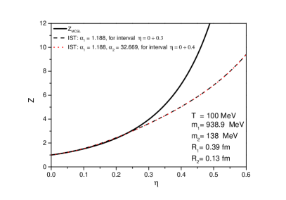
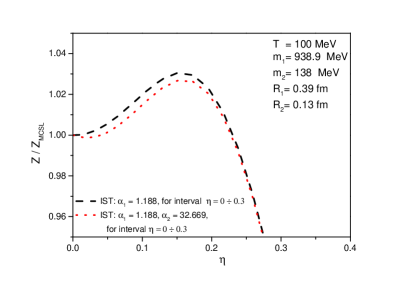
Figure 5: [Color online] Upper panel. Compressibility factors $Z$ of the two-component IST EoS and CS EoS (thick solid curve) with the best-fit parameters on interval of packing fraction $\eta\in[0.;0.3]$. The dashed curve corresponds to the case $\alpha_{2}=\alpha_{1}=1.188$ with $\tilde{\chi}^{2}\simeq 2.847$, while the dashed-dotted curve corresponds to the case $\alpha_{1}=1.188$, $\alpha_{2}=32.669$ and $\tilde{\chi}^{2}\simeq 2.523$. Lower panel. Same as in the upper panel, but for the ratios of the compressibility factors $Z/Z_{MCSL}$.

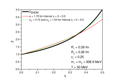
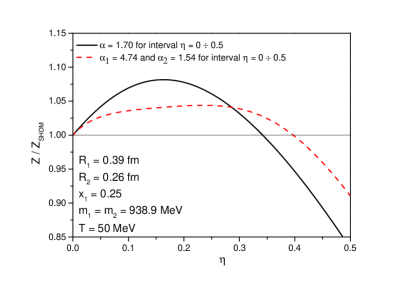
Figure 6: Upper panel. Compressibility factors $Z$ of the two-component IST EoS and SHDM EoS (thick solid curve) with the best-fit parameters on interval of packing fraction $\eta\in[0.;0.5]$. The thin solid curve corresponds to the case $\alpha_{2}=\alpha_{1}=1.7$ with $\tilde{\chi}^{2}\simeq 14.89$, while the dashed curve corresponds to the case $\alpha_{1}=4.74$, $\alpha_{2}=1.54$ and $\tilde{\chi}^{2}\simeq 4.48$. Lower panel. Similar to the upper panel, but for the ratios of the compressibility factors $Z/Z_{SHDM}$.

IV.2 Comparison with two-component EoS for hard discs

Also we compared the IST EoS with the Santos et al. (SHDM) EoS Santos1 for the compressibility factor of hard discs two-component mixture supplemented by the Woodcock EoS Woodcock which is used to model a compressibility of a single component EoS (for more details see Ref. SantosEoS )

$$Z_{SHDM} = \frac{(1-\xi)}{1-\eta}+\xi Z_{s}^{W}(\eta),$$ (49)

$$Z_{s}^{W}(\eta) = \frac{1+3\eta/\eta_{0}}{1-\eta/\eta_{0}}+\sum\limits_{n=2}^{6}(b_{n}\eta_{0}^{n-1}-4)\left[\frac{\eta}{\eta_{0}}\right]^{n-1},\leavevmode\nobreak\$$ (50)

where the variable

$$\xi=\left[\sum_{j=1}^{2}x_{j}\sigma_{j}\right]^{2}\left[\sum_{j=1}^{2}x_{j}\sigma_{j}^{2}\right]^{-1},$$ (51)

is expressed in terms of the molar fractions $x_{j}\equiv\rho_{j}/(\rho_{1}+\rho_{2})$ and the diameters $\sigma_{k}=2R_{k}$ of hard disc of sort $k$. Apparently, $\rho_{k}$ denotes the particle number density of the discs of sort $k$. The quantities $b_{n}$ ($n=2-6$) in Eq. (50) denote the reduced virial coefficients of hard discs Vir_Coeff_HD .

Since for the two-component case the SHDM EoS (49) requires a fixed concentration for each sort of discs, we also fix them as $x_{1}=0.25$ and $x_{2}=0.75$ for demonstration purpose. In addition, we implement an extra condition for the fixed ratio of discs diameters $\sigma_{2}/\sigma_{1}=2/3$ in order to make a detailed comparison with Ref. SantosEoS .

For 2-dimensional hadron gas of hard discs mixture of nucleons we used $m_{1}=m_{2}=939.8$ MeV and $\sigma_{1}=0.39$ fm, $\sigma_{2}=0.26$ fm. For such input we calculated the compressibility factor $Z$ for the IST and SHDM EoS and found the best-fit parameters on various intervals of packing fraction $\eta$. We considered the case of single $\alpha$ for both constituents and the case of multiple $\alpha_{1}$, $\alpha_{2}$. The results for the interval $\eta\in[0.;0.5]$ are shown in Fig. 6. As one can see the results found for a single value of $\alpha_{2}=\alpha_{1}$ are slightly worse than the ones obtained for the BS EoS shown in Figs. 3 and 4 for the case $\alpha_{1}=1.88$. For the case of $\alpha_{1}=4.74$ and $\alpha_{2}=1.54$ the results with $\tilde{\chi}^{2}\simeq 4.48$ as shown in Fig. 6 are comparable to the ones found for the BS EoS. In principle, the accuracy of few percent achieved by the IST EoS discussed above would be sufficient for the most practical applications in high energy nuclear physics, but in our opinion it is a clear signal that the IST concept has to be extended and supplemented by the curvature term.

V ISCT EoS for hard D-dimensional spheres

Let us begin this section from a formal analysis of the IH formula for the excluded volume of a pair of two convex hard particles. Introducing now the equivalent sphere radius as $S^{eigen}\equiv 4\pi R_{s}^{2}=S(R_{s})$ and doubled perimeters $C_{1}(\overline{R_{1}})=4\pi\overline{R_{1}}$ and $C_{2}(\overline{R_{2}})=4\pi\overline{R_{2}}$ defined for each mean radius of curvature $\overline{R_{k}}$ (with $k=1,2$) one can exactly rewrite the IH formula for a pair of identical convex hard particles as

$$2V_{excl}^{IH} \equiv \tilde{V}_{1}+a_{2}S(\overline{R_{1}})R_{s}+(1-\tilde{A})C_{1}(\overline{R_{1}})R_{s}^{2}$$ (52)

$$+ \tilde{V}_{2}+a_{2}S(\overline{R_{2}})R_{s}+(1-\tilde{A})C_{2}(\overline{R_{2}})R_{s}^{2},\quad$$

where the notations

$$\tilde{V}_{1} = V^{eigen}-\tilde{B}S(\overline{R_{1}})R_{s}(a_{1}-a_{2}),$$ (53)

$$\tilde{V}_{2} = V^{eigen}+(1+\tilde{B})S(\overline{R_{1}})R_{s}(a_{1}-a_{2}),$$ (54)

$$a_{k} \equiv \tilde{A}\frac{R_{s}}{\overline{R_{k}}}\quad{\rm with}\quad k=1,2,$$ (55)

are used. In Eqs. (52) and (53) the arbitrary constants $A$ and $B$ belong to the interval $[0;1]$. Writing the effective excluded volume for particles 1 and 2 from the equation for the pressure of ISCT EoS (36)

$$2V_{excl}^{eff}\equiv\frac{1}{p}\sum\limits_{k=1}^{2}\left[V_{k}p+S_{k}\Sigma+C_{k}K\right]=$$ (56)

$$=V_{1}+AS_{1}\overline{R}+BC_{1}\overline{R^{2}}+V_{2}+AS_{2}\overline{R}+BC_{2}\overline{R^{2}},\leavevmode\nobreak\$$ (57)

where in deriving Eq. (57) from (56) we used the definitions of $\overline{R}$ and $\overline{R^{2}}$ and Eqs. (37) and (38).

Comparing Eqs. (52) and (57) one can conclude that the both expressions have the same structure, if one identifies $R_{s}\Leftrightarrow\overline{R}$, $R_{s}^{2}\Leftrightarrow\overline{R^{2}}$, $a_{2}\Leftrightarrow A$ and $(1-\tilde{A})\Leftrightarrow B$. Moreover, this means that for low densities at which the EoS of hard spheres is defined by the second virial coefficient the ISCT EoS may be used not only for the hard spheres, but also for the convex hard particles. Besides, this comparison shows that the same excluded volume $V_{excl}^{IH}$ may be reproduced by many sets of parameters and, hence, one can use this freedom to accurately account for higher virial coefficients and not to spoil the description of the second one. Below we demonstrate this for 3- and 2-dimensional hard spheres.

For the one-component gas of hard spheres we found that the set of parameters $A=0.68$, $B=1-A$, $\alpha_{1}=1.14$ and $\beta=3.37$ the ISCT EoS exactly reproduces the 2-nd, 3-rd, 4-th and 5-th virial coefficients of the CS EoS. In Fig. 7 the ISCT EoS with such parameters is compared to the IST EoS found for the same value of parameter $\alpha_{1}=1.14$. As one can see from Fig. 7 for this set of parameters the ISCT EoS works very well up to the packing fraction $\eta\simeq 0.2$. Also from this figure one can see that the ISCT EoS with the best fit parameters $A=0.57$, $B=0.76$, $\alpha_{1}=1.07$ and $\beta_{1}=3.76$ is able to provide an essentially better description of the CS EoS for the packing fractions $\eta\leq 0.45$ with $\tilde{\chi}^{2}=0.6$. In other words, the ISCT EoS is able to describe the compressibility of the whole gaseous phase of hard spheres using four parameters only. This is highly nontrivial result, since a comparable quality of description can be achieved by more than 10 virial coefficients of hard spheres. The results for a one-component gas of hard discs are very similar and, hence, they are not shown.

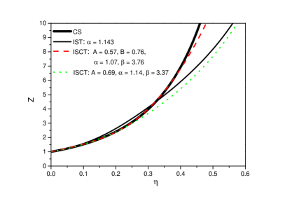
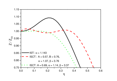
Figure 7: [Color online] Upper panel. Comparison of the compressibility factors $Z$ of the CS EoS (solid thick curve) with the one-component IST EoS with best-fit parameters on interval of packing fraction $\eta\in[0.;0.4]$ (from Fig. 1,2) (solid thin curve), the ISCT EoS with best-fit parameters on the same interval with $\tilde{\chi}^{2}\simeq 0.60$ (dashed curve) and the ISCT EoS which exactly reproduces the five virial coefficients of the CS EoS (dotted curve). Lower panel. Same as in the upper panel, but for the ratios of the compressibility factors $Z/Z_{CS}$.

It is interesting that the one-component ISCT EoS may help to qualitatively understand the reason of why the surface tension of small metallic nano-particles of radius $R_{1}$ demonstrates the linear dependence on their radius which is justified theoretically in Refs. NanoPart1 ; NanoPart2 . Indeed, considering the dense gas of hard metallic spheres close to its solid state from Eq. (37) one can immediately see that the surface tension coefficient $\Sigma\simeq R_{1}F(p,T)$ linearly depends on the radius of hard spheres and on system pressure $p$ and its temperature $T$. Of course, the attraction which exists among the nano-particles studied in Refs. NanoPart1 ; NanoPart2 may be important, but, perhaps, for small values of $R_{1}$ the repulsive effects dominate and, hence, the hard-core repulsion manifests itself via the linear dependence of surface tension coefficient on $R_{1}$.

Now we turn to the analysis of two-component case. The ISCT EoS results obtained for the mixture of nucleons and pions studied in preceding sections are shown in Fig. 8. This figure shows one that the two-component CS EoS (47) is very well reproduced by the ISCT EoS on intervals of packing fraction $\eta=0.4-0.45$, i.e. almost for an entire gaseous phase of hard spheres. The best fit parameters of ISCT EoS which correspond to Fig. 8 are given in Table 1. Note that only with two additional parameters compared to the one-component case we obtained even better quality of the fit.

Table 1: The best fit parameters of the ISCT EoS which reproduce the MCSL EoS on two intervals. The upper row corresponds to to the fitting interval $\eta\in[0.;0.45]$, while the lower one provides an excellent description at the interval $\eta\in[0.;0.35]$.

$\alpha_{1}$	$\alpha_{2}$	$\beta_{1}$	$\beta_{2}$	$A$	$B$	$\tilde{\chi}^{2}$	$\eta$
1.050	1.007	2.084	1.862	0.442	0.630	0.23	0 - 0.45
1.070	1.012	2.428	2.372	0.520	0.512	0.02	0 - 0.35

Fig. 9 shows one the ratio of ISCT EoS compressibility factor $Z$ for two-component hadron gas of hard discs to the one of the SHDM EoS (49) with the best-fit parameters up to $\eta=0.7$ for the case analyzed in Section (IV.2). In 2-dimensional case the ISCT EoS gives even more notable improvement compared to the IST EoS results than in 3-dimensional case. Remarkably, it allows us to extend the description of two-component SHDM EoS (49) up to $\eta=0.7$, i.e. for the whole gaseous phase with $\sqrt{\tilde{\chi}^{2}}\simeq 0.7$ percent (see the case $\alpha_{1}=1.076$ and $\alpha_{2}=1.575$ in Fig. 9 and in Table 2.

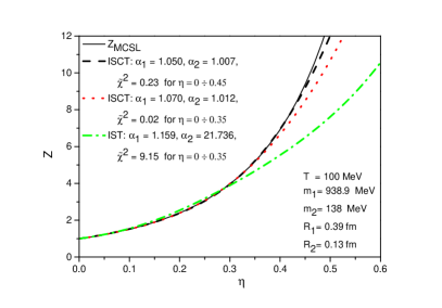
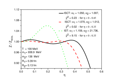
Figure 8: Upper panel. Comparison of the compressibility factors with the best-fit parameters obtained with IST and ISCT EoS for hard spheres gas with multicomponent CS EoS $Z_{MCSL}$ MCSL . Lower panel. Similar to the upper panel, but for the ratios of the compressibility factors $Z/Z_{MCSL}$ (All parameters are given in Table. 1).

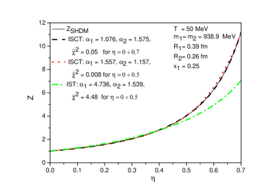
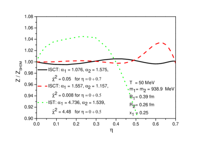
Figure 9: Upper panel. Comparison of the compressibility factors with the best-fit parameters obtained with IST and ISCT EoS for hard discs mixture with multicomponent SHDM EoS $Z_{SHDM}$ SantosEoS . Lower panel. Same as in the upper panel, but for the ratios of the compressibility factors $Z/Z_{SHDM}$ (All parameters are given in Table. 2).

Table 2: The best fit parameters of the ISCT EoS which reproduce the SHDM EoS on two intervals. The upper row corresponds to to the fitting interval $\eta\in[0.;0.7]$, while the middle one provides an excellent description at the interval $\eta\in[0.;0.5]$. The lowest row corresponds to the IST EoS with the case $\alpha_{2}\neq\alpha_{1}$.

$\alpha_{1}$	$\alpha_{2}$	$\beta_{1}$	$\beta_{2}$	A	B	$\tilde{\chi}^{2}$	$\eta$
1.076	1.575	1.587	1.392	0.176	0.276	0.05	0 - 0.7
1.557	1.157	3.009	3.008	0.504	-0.0099	0.008	0 - 0.5
4.736	1.539					4.48	0 - 0.5

VI Discussion of results and perspectives

In this work we analyzed the excluded volume of the multicomponent mixtures of hard spheres and hard discs. With the help of the self-consistent approximation we derived the system of equations for the IST and ISCT EoS which define the surface tension coefficient generated by the hard-core repulsion for the IST and ISCT EoS and the induced curvature tension coefficient for the ISCT case. In order to extend the applicability range of the IST approach one has to include into the treatment the curvature tension coefficient. This is done in a general way by requiring that the relative importance of surface and curvature tensions compared to the pressure should weaken at high packing fractions. In practice, we suggest modifying the distribution functions entering the expressions for the induced surface and curvature tension coefficients in order to account for higher virial coefficients of the multicomponent mixtures while keeping the correct values of the second virial coefficients.

A comparison of the obtained ISCT EoS with the well-known one-component Carnahan-Starling EoS for hard spheres and Barrio-Solana EoS for hard discs showed us that it is possible to accurately describe the compressibility factors of these equations for $\eta\leq 0.3$ and $\eta\leq 0.5$, respectively. Basically the same results are found for the two-component EoS of hard spheres and hard discs, if one describes them by the IST EoS. However, we found that the ISCT EoS is able to essentially improve the description of one- and two-component gases of hard spheres and hard discs and to extend it to the entire gaseous phase with the accuracy which exceeds the experimental abilities of modern nuclear physics of intermediate and high energies.

The fact that the same system of equations with the same number of phenomenological parameters, i.e. the ISCT EoS, is able to accurately reproduce the well-known EoS of one- and two-component gases of hard spheres and hard discs evidences that the concept of ISCT captures the correct physics in the grand canonical ensemble. The great advantage of the IST and ISCT EoS for multicomponent mixtures compared to the other multicomponent EoS is that the number of equations which are necessary to be solved does not depend on the number of different hard-core radii in the considered system. Therefore, the IST and ISCT can be used to formulate the more realistic exactly solvable models with the first order liquid-gas phase transition in ordinary liquids, in nuclear liquid and in hadronic matter in order to improve the existing approaches (see, for instance, Refs. IST1 ; Reuter08 ; NewFisher1 ; NewFisher2 ; SMM1 and references therein). As it was mentioned above the ISCT EoS can also be used to improve the model of surface deformations of physical clusters and to find out their surface entropy in a spirit of exactly solvable models of Refs. HDM1 ; HDM2 .

Based on the mathematical similarity between the IH formula for the second virial coefficient of convex hard particles and the expression for the excluded volume of two-component mixture obtained here we argue that after some modification the ISCT EoS can be used to model the multicomponent mixtures of convex hard particles of different shapes and sizes. Therefore, this direction of research may be useful to many practical applications for which the exact treatment of EoS is mathematically too complicated, but comparatively simple numerical analysis like the molecular dynamics can provide us with a few virial coefficients of multicomponent mixtures. Clearly, the grand canonical treatment of such multicomponent mixtures will be a good addition and alternative to the well known EoS of multicomponent mixtures of convex hard particles of different shapes and sizes obtained in the canonical ensemble in Refs. Carnahan0 ; Carnahan1 ; Carnahan2 . Also, it is apparent that the mathematical scheme outlined here can be generalized to take into account for the attraction between the constituents. It is, however, clear that at low packing fractions such an attraction will decrease the value of induced surface curvature coefficient, while its effect on the curvature tension coefficient may depend on the attractive potential.

The recent analysis of the quantum hard spheres QSTAT2019 shows that the set of equations which are found directly from the quantum partition function of a multicomponent mixture of hard spheres leads, in general, to a different (and essentially more complicated) set of equations for the quantities $\overline{R}$ and $\overline{R^{2}}$ than the one derived here. Nevertheless, in Ref. QSTAT2019 it is shown that at low densities the quantum equations coincide with the ones derived here for the induced surface tension coefficient $\Sigma\equiv A\overline{R}p$ and for the curvature tension one $K\equiv B\overline{R^{2}}p$. Furthermore, as it is argued in QSTAT2019 the multicomponent quantum VdW EoS with the hard-core repulsion is so complicated that instead of its extrapolation to high densities it is more instructive to extrapolate the quantum analog of the system (33)-(35) to high densities. Therefore, the equations for the induced surface tension coefficient $\Sigma\equiv A\overline{R}p$ and for the curvature tension one $K\equiv B\overline{R^{2}}p$ derived here for the multicomponent VdW EoS with the hard-core repulsion may be also important for formulating the realistic quantum EoS of multicomponent mixtures of hard discs, hard spheres and hard hyper-spheres of higher spatial dimensions.

Acknowledgments. The authors are thankful to B. E. Grinyuk, O. I. Ivanytskyi, V.V. Sagun, S. N. Nedelko, E. G. Nikonov and G. M. Zinovjev for fruitful discussions and valuable comments. The work of K.A.B. was supported by the Program of Fundamental Research in High Energy and Nuclear Physics launched by the Section of Nuclear Physics of the National Academy of Sciences of Ukraine. The work of L.V.B. and E.E.Z. was supported by the Norwegian Research Council (NFR) under grant No. 255253/F53 CERN Heavy Ion Theory. N.S.Ya., L.V.B. and K.A.B. thank the Norwegian Agency for International Cooperation and Quality Enhancement in Higher Education for the financial support under grant CPEA-LT-2016/10094 “From Strong Interacting Matter to Dark Matter”. K.A.B. is also grateful to the COST Action CA15213 “THOR” for supporting his networking.

Appendix: Expressions for particle density

Appendix A Formulae for IST EoS

In order to compare the IST EoS with the Mansoori-Carnahan-Starling-Leland EoS MCSL we need to have the explicit expressions for the particle number density of the $k$-th sort of particles. Hence, we consider the system (23) and (26), i.e., the partial pressure $p_{k}$ and the partial surface-tension coefficient $\Sigma_{k}$ are defined as

$$p_{k} = T\phi_{k}\exp\left[\frac{\mu_{k}}{T}-v_{k}\frac{p}{T}-s_{k}\frac{\Sigma}{T}\right]\,,$$ (58)

$$\Sigma_{k} = TR_{k}\phi_{k}\exp\left[\frac{\mu_{k}}{T}-v_{k}\frac{p}{T}-s_{k}\alpha_{k}\frac{\Sigma}{T}\right]\leavevmode\nobreak\ \quad$$ (59)

$$\equiv p_{k}R_{k}\exp\left[-s_{k}(\alpha_{k}-1)\frac{\Sigma}{T}\right]\,.$$ (60)

Then the total pressure and the total surface tension coefficient are defined as $p=\sum_{k}p_{k}$ and $\Sigma=\sum_{k}\Sigma_{k}$, respectively. In the 3-dimensional case (hard spheres) $v_{k}=\frac{4}{3}\pi R_{k}^{3}$ and $s_{k}=4\pi R_{k}^{2}$, while in the 2-dimensional case (hard discs) $v_{k}=\pi R_{k}^{2}$ and $s_{k}=2\pi R_{k}$.

Differentiating $p$ and $\Sigma$ with respect to the full chemical potential $\mu_{k}$ of the hadron of sort $k$ one finds

$$\begin{pmatrix}a_{11}&a_{12}\\ a_{21}&a_{22}\end{pmatrix}\cdot\begin{pmatrix}\frac{\partial p}{\partial\mu_{k}}\\ \frac{\partial\Sigma}{\partial\mu_{k}}\end{pmatrix}=\begin{pmatrix}\frac{p_{k}}{T}\\ \frac{\Sigma_{k}}{T}\end{pmatrix}$$ (61)

The coefficients $a_{kl}$ can be expressed in terms of the partial pressures $\{p_{k}\}$ and the partial surface tension coefficients $\{\Sigma_{k}\}$ as

$$a_{11}=1+\sum_{k}v_{k}\frac{p_{k}}{T}\,, a_{12}=\sum_{k}s_{k}\frac{p_{k}}{T}\,,$$ (62)

$$a_{21}=\sum_{k}v_{k}\frac{\Sigma_{k}}{T}\,, a_{22}=1+\sum_{k}s_{k}\alpha_{k}\frac{\Sigma_{k}}{T}\,.\quad$$ (63)

Then the particle number density of $k$-th sort of particle is given by

$$\rho_{k}\equiv\frac{\partial p}{\partial\mu_{k}}=\frac{1}{T}\cdot\frac{p_{k}\,a_{22}-\Sigma_{k}\,a_{12}}{a_{11}\,a_{22}-a_{12}\,a_{21}}\,.$$ (64)

Appendix B Useful formulae for ISCT EoS

Similarly to the IST EoS, one can calculate particle number densities for ISCT EoS. The corresponding coefficients are expressed in terms of partial quantities $\{p_{k}\}$, $\{\Sigma_{k}\}$ and $\{K_{k}\}$ as

$$a =1+\sum_{k}\alpha_{k}s_{k}\frac{\Sigma_{k}}{T}\,, b =\sum_{k}v_{k}\frac{\Sigma_{k}}{T}\,, c =\sum_{k}c_{k}\frac{\Sigma_{k}}{T}\,,$$

$$d =1+\sum_{k}\beta_{k}c_{k}\frac{K_{k}}{T}\,, e =\sum_{k}v_{k}\frac{K_{k}}{T}\,, f =\sum_{k}\alpha_{k}s_{k}\frac{K_{k}}{T}\,,$$

$$g =1+\sum_{k}v_{k}\frac{p_{k}}{T}\,, h =\sum_{k}s_{k}\frac{p_{k}}{T}\,, j =\sum_{k}c_{k}\frac{p_{k}}{T}\,.$$

Then for the ISCT EoS the particle number density of the $k$-th sort of particles is given by

$$\rho_{k}=\frac{1}{T}\frac{(ad-cf)p_{k}-(dh-fj)\Sigma_{k}+(ch-aj)K_{k}}{g(ad-cf)-b(dh-fj)+e(ch-aj)}\,.$$ (65)

In the 3-dimensional case (hard spheres) $v_{k}=\frac{4}{3}\pi R_{k}^{3}$, $s_{k}=4\pi R_{k}^{2}$ and $c_{k}=4\pi R_{k}$, while in the 2-dimensional case (hard discs) $v_{k}=\pi R_{k}^{2}$, $s_{k}=2\pi R_{k}$ and $c_{k}=2\pi$.

References

- (1) A. Isihara, J. Chem. Phys. 18, 1446 (1950).
- (2) H. Hadwiger, Mh. Math. 54, 345 (1950).
- (3) A. Isihara, Statistical physics (Academic Press, New York, 1971).
- (4) J. P. Hansen and I. R. McDonald, Theory of Simple Fluids (Academic Press, Amsterdam, 2006).
- (5) V. V. Sagun, A. I. Ivanytskyi, K. A. Bugaev and I. N. Mishustin, Nucl. Phys. A 924, 24 (2014).
- (6) K. A. Bugaev et al., Nucl. Phys. A 970, 133 (2018).
- (7) V. V. Sagun et al., Eur. Phys. J. A 54, 100 (2018).
- (8) A. I. Ivanytskyi, K. A. Bugaev, V. V. Sagun, L. V. Bravina and E. E. Zabrodin, Phys. Rev. C 97, 064905 (2018).
- (9) V. V. Sagun, I. Lopes and A. I. Ivanytskyi, Astrophys. J. 871, 157 (2019).
- (10) V. Sagun, I. Lopes and A. Ivanytskyi, Nucl. Phys. A 982, 883 (2019).
- (11) K. A. Bugaev et al., Phys. Part. Nucl. Lett. 15, 210 (2018).
- (12) K. A. Bugaev, A. I. Ivanytskyi, V. V. Sagun, E. G. Nikonov and G. M. Zinovjev, Ukr. J. Phys. 63, 863 (2018).
- (13) N. F. Carnahan and K. E. Starling, J. Chem. Phys. 51, 635 (1969).
- (14) M. Lopez de Haro, S. B. Yuste and A. Santos, Phys. Rev. E 66, 031202 (2002).
- (15) C. Barrio and J. R. Solana, Phys. Rev. E 63, 011201 (2001).
- (16) J. Schukraft, Nucl. Phys. A 967, 1 (2017).
- (17) K. A. Bugaev and P. T. Reuter, Ukr. J. Phys. 52, 489 (2007) and references therein.
- (18) K. Huang, Statistical Mechanics (Wiley & Sons, 1967)
- (19) M. Brack, C. Guet and H.-B. H/okansson, Phys. Rep. 123, 276 (1984) and references therein.
- (20) K. Pomorski and J. Dudek, Phys. Rev. C 67, 044316 and references therein.
- (21) V. M. Kolomietz, S. V. Lukyanov and A. I. Sanzhur, Phys. Rev. C 86, 024304 (2012) and references therein.
- (22) L. G. Moretto, P. T. Lake and L. Phair, Phys. Rev. C 86, 021303(R) (2012) and references therein.
- (23) V. V. Sagun, K. A. Bugaev and A. I. Ivanytskyi, Phys. Part. Nucl. Lett. 16, 671 (2019).
- (24) M. E. Fisher, Physics 3, 255 (1967).
- (25) A. Dillmann and G.E. Meier, J. Chem. Phys. 94, 3872 (1991).
- (26) A. Laaksonen, I.J. Ford and M. Kulmala, Phys. Rev. E 49, 5517 (1994) and references therein.
- (27) M. N. Bannerman, L. Lue, and L. V. Woodcock, J. Chem. Phys. 132, 084507 (2010).
- (28) K. A. Bugaev, L. Phair and J. B. Elliott, Phys. Rev. E 72, 047106 (2005).
- (29) K. A. Bugaev and J. B. Elliott, Ukr. J. Phys. 52, 301 (2007).
- (30) G. A. Mansoori, N. F. Carnahan, K. E. Starling, T. Leland, J. Chem. Phys. 54, 1523, (1971).
- (31) A. Santos, S. B. Yuste, and M. Lopez de Haro, Mol. Phys. 96, 1 (1999).
- (32) L. V. Woodcock, J. Chem. Soc., Faraday Trans. 2 72, 731 (1976).
- (33) E. J. J. van Rensburg, J. of Physics A 26, 4805 (1993).
- (34) V. M. Samsonov, A. N. Bazulev and N. Yu. Sdobnyakov, Central Europ. J. Phys. 1, 474 (2003) and references therein.
- (35) V. M. Samsonov, A. A. Chernyshova and N. Yu. Sdobnyakov, Izv. RAN, Ser. Physics. 80, 768 (2016) (in Russian) [DOI: 10.7868/S0367676516060296] and references therein.
- (36) K. A. Bugaev, M. I. Gorenstein, I. N. Mishustin and W. Greiner, Phys. Rev. C 62, 044320 (2000).
- (37) N. F. Carnahan, Mller and J. Pikunic, Phys. Chem. Chem. Phys., 1999, 1, 4259.
- (38) L. V. Yelash, Th. Kraska, E. A. Mller and N. F. Carnahan, Phys. Chem. Chem. Phys. 1, 4919 (1999).
- (39) N. F. Carnahan and E. A. Mller, Phys. Chem. Chem. Phys. 8, 2619 (2006).
- (40) K. A. Bugaev, arXiv:1907.09931v1 [cond-mat.sta-mech].