Place Deduplication with Embeddings

Abstract.

Thanks to the advancing mobile location services, people nowadays can post about places to share visiting experience on-the-go. A large place graph not only helps users explore interesting destinations, but also provides opportunities for understanding and modeling the real world. To improve coverage and flexibility of the place graph, many platforms import places data from multiple sources, which unfortunately leads to the emergence of numerous duplicated places that severely hinder subsequent location-related services. In this work, we take the anonymous place graph from Facebook as an example to systematically study the problem of place deduplication: We carefully formulate the problem, study its connections to various related tasks that lead to several promising basic models, and arrive at a systematic two-step data-driven pipeline based on place embedding with multiple novel techniques that works significantly better than the state-of-the-art.

ACM Reference Format:
Carl Yang, Do Huy Hoang, Tomas Mikolov, Jiawei Han. 2019. Place Deduplication with Embeddings. In Proceedings of the 2019 World Wide Web Conference (WWW’19), May 13-17, 2019, San Francisco, CA, USA. ACM, New York, NY, USA, 7 pages. https://doi.org/10.1145/3308558.3313456

1. Introduction

With the prevalence of mobile devices and online social platforms, maps and location related apps have become an integral part of people’s everyday life. It has encouraged the development of various location-oriented infrastructures and services (Lian et al., 2014; Li et al., 2015; Ye et al., 2011; Liu et al., 2014; Ference et al., 2013; Sarwat et al., 2014; Yin et al., 2015). For most of them, one key task is the maintenance of a high-quality map database (a.k.a. place graph), which consists of various real-world places and their attributes. On one hand, such a database can support various map-based activities like search, like, check-in and post. Improving the efficiency and quality of such activities is beneficial to various stakeholders including business owners, advertisement agencies, and common users. On the other hand, the frequent location-based activity data generated by users provide an invaluable opportunity to improve the representation and understanding of the real world, and may further shed light on the capturing and modeling of various real-world activities.

However, since place pages are usually created from multiple sources whose qualities are hard to verify upon creation, the place graphs are often subject to large amounts of duplications, which hurts the quality of subsequent location-based services. For example, when a user touring in New York City wants to make a post at Times Square, if the system returns a list of places like “New York Time Square” “Manhattan, Time Square” “TimeSquare, NYC”, the user will get confused about which one to post on. Worse still, if the user also wants to explore restaurants or shopping malls around Times Square, then she/he may need to manually combine multiple lists of stores to get a full picture of all available choices.

Such user experiences are mainly due to the problem of duplicated places. To ease users’ exploration of places and sharing of experiences, in this work, we take the massive anonymous place graph from Facebook as an example to systematically study the problem of place deduplication, and comprehensively evaluate the performance of different methods through extensive experiments on duplication candidate fetch and pair-wise duplication prediction.

Specifically, we start with large-scale unsupervised feature generation to encode various ad-hoc place attributes through embedding learning and network-based embedding smoothing. Upon that, we develop an effective supervised metric learning framework to find the most useful features indicating place duplications. To fully leverage the noisy labeled data, we novelly pack the model with a series of techniques including batch-wise hard sampling, source-oriented attentive training, and soft clustering-based label denoising. Extensive experiments on real-world place data show that our pipeline can outperform state-of-the-art industry-level baselines by significant margins, while each of our novel model components effectively pushes the limit of the overall pipeline.

Note that, although we focus on the example of Facebook data, our place deduplication pipeline is general and ready to be applied to any online platform with place data or other deduplication tasks. Full implementation of our place embedding pipeline based on PyTorch will be released after the acceptance of this work.

2. Problem Formulation

Nowadays, many online platforms maintain a place graph to map the real world. The building blocks of such place graphs, however, instead of actual places, are usually online place pages that capture certain attributes of actual places, as illustrated in Figure 1. Since such online places can be created by users, imported from third-party companies or scraped from the Web, many of them are duplicated, as they in fact describe the same real-world places. In this work, to improve the quality of place graphs, we aim at the following novel but emergent problem.

Definition 2.1.

Place Deduplication. Given a large set of online place pages, find those describing the same real-world places.

Input.

Given a set of online places $\mathcal{P}$, we represent the attributes of each place $p_{i}\in\mathcal{P}$ as $\mathbf{a}_{i}\in\mathcal{A}$. Such attributes can be ad-hoc, for example, place names, addresses, phone numbers, visitor histories, images, relevant posts and so on, which are essentially combinations of numerical, categorical, textual and even visual features. Moreover, due to the reality, many attributes can be missing and inaccurate.

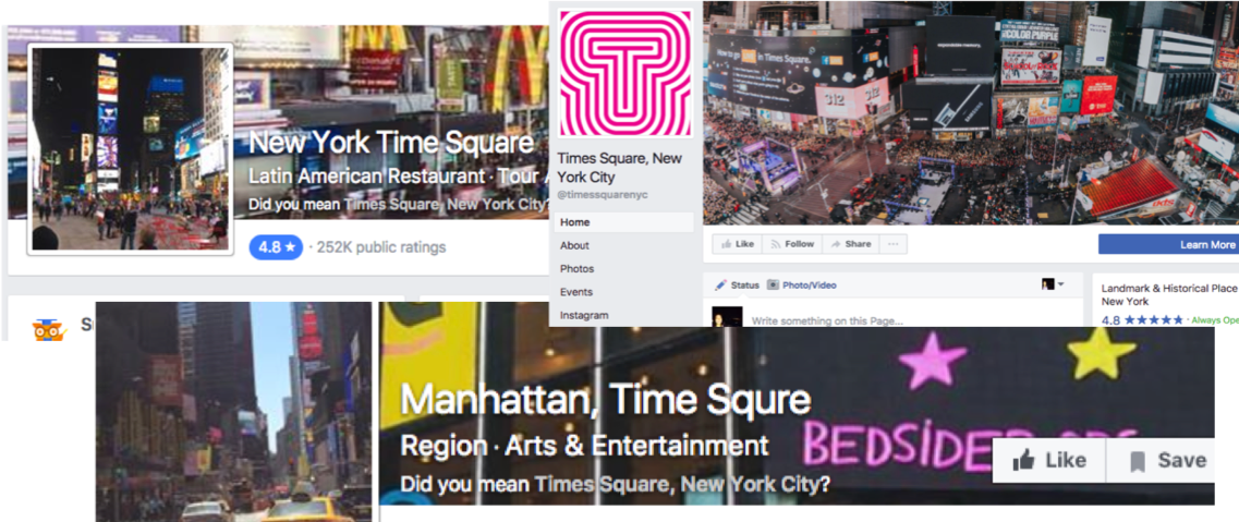
Figure 1. Example input with ad-hoc page features.

Output.

For each place $p_{i}\in\mathcal{P}$, we aim to compute a unique fixed-sized low-dimensional vector (a.k.a. embedding) $\mathbf{u}_{i}\in\mathcal{U}$, to encode its ad-hoc attributes $\mathbf{a}_{i}\in\mathcal{A}$. After getting such embeddings, various related tasks can be efficiently addressed through off-the-shelf machine learning algorithms. For example, duplication candidate fetch (find places that may be potentially duplicated) can be done through fast $k$-NN search (Garcia et al., 2008; Johnson et al., 2017), pair-wise duplication prediction (decide if two places are duplications) simply involves the computation of pair-wise Euclidean distances, and meta-page discovery (find common actual places among all online places) can be achieved using clustering techniques such as $k$-means (Han et al., 2011).

Labels.

To learn the proper place embedding $\mathcal{U}$ that facilitates place deduplication, besides place attributes $\mathcal{A}$, we also aim to leverage some labeled data $\mathcal{L}$, which are mainly from curation, crowdsourcing, and feedbacks. The labels are usually in the form of place pairs like $l=\{(a,b),y_{l}\}$, where $a$ and $b$ are two probe places. $y_{l}=1$ denotes a positive pair, meaning $a$ and $b$ are labeled as duplications, and $y_{l}=0$ denotes a negative pair. Labels from different sources can have varying qualities and biases.

Present work.

Taking the ad-hoc raw place attributes $\mathcal{A}$, we firstly transform them into fixed-sized numerical vectors $\mathcal{X}$ with unsupervised learning techniques, which captures the key information in $\mathcal{A}$ and can be easily processed by subsequent machine learning algorithms. Guided by labeled place pairs in $\mathcal{L}$, we then explore the feature representation $\mathcal{X}$ through supervised learning techniques and learn the final place embeddings $\mathcal{F}$ as vectors in a metric space where labeled duplicated places are close and non-duplicated places lie far apart. While we focus on place deduplication, the concepts and methods developed in this work are not bounded to the particular problem, but can be generally useful for deduplicating various objects like texts and users with similar types of attributes.

3. Related Work and Motivations

We find the place deduplication problem closely related to several key tasks that heavily rely on advanced machine learning techniques, especially in the domains of computer vision (CV) and natural language processing (NLP).

3.1. CV: Person Re-Identification

One of the key tasks in CV is person re-identification (Chen et al., 2017; Ding et al., 2015; Chen et al., 2016; Cheng et al., 2016; Su et al., 2016; Wang et al., 2016), also referred to as face recognition (Schroff et al., 2015; Sun et al., 2015; Taigman et al., 2014). Given a large number of human images, the task is to find images of the same person. In concept, this task is quite close to ours as defined in Section 2.

In CV, mainstream algorithms often tackle re-identification by projecting the images into a latent embedding space, while tuning the embedding space based on labeled data with a triplet loss to enforce the correct order for each probe image. Their conceptual optimization objective can be expressed as follows.

(1) $$\mathcal{J}_{tr}=\sum_{t=(a,p,n)} \text{max}(0,d(\mathbf{u}_{a},\mathbf{u}_{p})-d(\mathbf{u}_{a},\mathbf{u}_{n})+\alpha),$$

where $\mathbf{u}=\mathbf{f}(\mathbf{x})$ and $d(\mathbf{u}_{i},\mathbf{u}_{j})=d_{e}(\mathbf{u}_{i},\mathbf{u}_{j})=||\mathbf{u}_{i}-\mathbf{v}_{j}||_{2}^{2}$. $\mathbf{x}$ is the original image features (e.g., $96\times 96$ pixels), $\mathbf{f}(\cdot)$ denotes the embedding projection function (e.g., a deep CNN), $\alpha$ is the margin hyper-parameter, and $||\cdot||_{2}^{2}$ denotes the Frobenius norm.

However, while images naturally come with rich visual features that can be well explored by the CNN models, the attributes of our places are much more ad-hoc and hard to capture. Another limitation of their models is the requirement of training data to be accurate and in the form of triplets, i.e., $t=(a,p,n)$, where $a$ is the probe image, $p$ is the positive image and $n$ is the negative image. In person re-identification, the labels are often generated from image collections taken of the same persons. Therefore, while the quality of input images may be different, the labels are often accurate, and the triplet requirement is easy to be satisfied.

In our scenario of place deduplication, labels are generated from different sources like curation and crowdsource based on samples of all possible place pairs, and are thus prone to varying qualities and biases. Moreover, instead of triplets, the training data naturally come as pairs, in the form of $l=\{(a,b),y_{l}\}$, as defined in Section 2. Finally, place duplication labels are extremely sparse– in our case, only about $10^{-5}$ percent of place pairs are labeled. It requires non-trivial adaptions of the CV models to work for place deduplication, which we will talk about in Section 5 and 6.

3.2. NLP: Entity Resolution

If we only consider place names, the problem is close to synonym detection. However, as most algorithms leverage sentence-level contexts to learn word similarities (Ustalov et al., 2017; Qu et al., 2017; Roller et al., 2014; Weeds et al., 2014; Qian et al., 2009; Sun and Grishman, 2010), they are not directly applicable to place deduplication where such contexts are often not available. Instead, we may consider direct matching of place names, which can be done using deep neural networks (Hu et al., 2014; Wan et al., 2016; Sun and Wu, 2018; Guo et al., 2016; Xiong et al., 2017; Pang et al., 2016; Chen et al., 2018). However, these models are known to be more suitable for longer sentences with more complex structures, rather than the short simple place names, and they require large amounts of training data, which is extremely hard to acquire for place deduplication (Christen et al., 2015; Dal Bianco et al., 2016; Qian et al., 2017). Finally, by considering additional place attributes like location, ad-hoc models have been developed based on heuristic feature engineering (Dalvi et al., 2014; Chuang and Chang, 2015; Kozhevnikov and Gorovoy, 2016), but their flexibility is limited to take more different place attributes, such as address and category. Thus, it is desirable for us to develop our own systematic and flexible place deduplication pipeline beyond the existing works on entity resolution, as we will discuss in Section 5 and 6.

Interestingly, another particular trend of entity resolution is to construct the word networks from search engine query logs and compute network clustering to detect synonym sets (He et al., 2016; Ren and Cheng, 2015; Chakrabarti et al., 2012). Since it is non-trivial to put everything we have into a single network, their methods are not directly applicable. Nonetheless, we find the ideas of network construction and clustering intriguing, and are able to leverage both of them in Section 5 and 6, respectively.

4. Data and Experimental Setups

In this section, we describe the massive dataset we use, upon which place deduplication is desired. It is a subset of the anonymous real-world place graph from Facebook including a total of 730M online place pages. In this work, we take the Facebook place graph as an example to show the effectiveness and efficiency of the methods we develop, while they are generally applicable to any online platforms with place data or other deduplication tasks.

4.1. Data Preparation

As we discussed in Section 2, places can have various ad-hoc attributes with varying qualities and incompleteness, which need to be leveraged through specifically designed methods, as we will show in Section 5.

We process and generate training data of about 4.6M pairs of places from 19 different sources, including curation, crowdsourcing, feedbacks and so on. Labels from curation are generally of higher qualities, while most of the others like feedbacks generated through surveys and crowdsourcing produced by cheap labors may be rather noisy. They cover a total of about 4M places. Among them, about 1.1M pages are labeled with duplications and 3M pages with non-duplications. The average number of duplications is 0.35, whereas the maximum number of duplications is 297. The average number of non-duplications is 1.98, and the maximum number of non-duplications is over 1K. Therefore, the training data are sparse and biased, and such sparsity and bias are different across the sources. In Section 6, we will discuss how to leverage such training data with varying noise, sparsity, and bias.

4.2. Evaluation Methods

The testing data we use is a golden set of 47K pages completely separate from the training data, which is deliberately curated for place quality evaluation for production. It contains different place pages from the training data.

To compare different embedding models, we firstly compute the vector representations $\mathcal{U}$ of all places in the testing set. For the set of places labeled with both duplications and non-duplications (i.e., $a\in\Omega$), we compute the average pair-wise accuracy as follows:

$$\text{ACC}=\frac{1}{|\Omega|}\sum_{a\in\Omega}\frac{1}{|\Phi_{a}||\Psi_{a}|}\sum_{p\in\Phi_{a},n\in\Psi_{a}}\mathbb{I}(||\mathbf{u}_{a}-\mathbf{u}_{p}||_{2}^{2}<||\mathbf{u}_{a}-\mathbf{u}_{n}||_{2}^{2}),$$

where $\Phi_{a}$ and $\Psi_{a}$ are the sets of labeled duplications and non-duplications of place $a$, respectively. This metric measures the utility of the embedding for the task of pair-wise duplication prediction.

Besides ACC, we also compute the nearest neighbors of each place through fast $k$-NN (Johnson et al., 2017), and compute the precision and recall at $K$ based on the set of places labeled with duplications (i.e., $a\in\Theta$), to measure the utility of the embedding for the task of point-wise duplication candidate fetch.

5. Unsupervised Feature Generation

The key place attributes we aim to leverage in this work are name, address, coordinate and category, while other attributes can also be easily incorporated in the future. Among them, name and address are textual, coordinate is numerical, and category is categorical, which need to be handled differently. Moreover, many of them are noisy and incomplete, requiring the model to be robust and flexible.

5.1. Encoding Name

We start with place name, because it is often the primary and most indicative feature towards deduplication(e.g., “Metropolitan Museum of Art” and “The MET”). Motivated by the success of word embedding in NLP, we propose to capture the place name semantics through embedding. The idea is to leverage the distributional information about words and infer word semantic similarities based on the context, so as to recognize common misspellings (e.g., “capitol” as “capital”, “corner” as “conner”), acronyms (e.g., “street” as “st”), synonyms (e.g., “plaza” and “square”) and etc.

Method 1: Skip-gram + place name corpus.

We firstly train a simple word embedding model on all place names we have, which include 730M short texts. For preprocessing, we prune all place names into the shortest name variants by removing all location prefixes and suffixes in the names (e.g., remove “New York” from “Time Square New York”); we also normalize all place names by replacing special characters with spaces (e.g., replace “$” or emojis with a single space) and change all letters to lower cases.

Since place names are often quite short (on average only 3.11 words after preprocessing), we directly apply the Skip-gram model (Mikolov et al., 2013) by sampling word-context pairs from place names. Place embedding is then computed as the average of word embedding.

This method, while efficiently providing numerical place name representations that can be processed by subsequent machine learning algorithms, has quite a few drawbacks as listed below.

• Limited distributional information: The training corpus, although is quite large, provides rather limited statistics around words and their contexts, since the corpus is chunked into short texts.

• Biased samples: Unlike sampling word-context pairs from fixed-sized sliding windows, when sampling from the place names, it is hard to avoid the bias towards either shorter or longer names.

• Ignorance of word internal structure: Standard word vectors ignore word internal structure that contains rich information, which might be especially useful for rare or misspelled words.

Method 2: Fast-text + Facebook post corpus.

To ameliorate the above limitations, we adopt the advanced Fast-text method (Mikolov et al., 2018), with strategies including position-dependent weighting, phrase generation and subword enrichment (Bojanowski et al., 2017; Joulin et al., 2017). Moreover, to capture more casual languages used by social network users who frequently create the place pages, instead of training the Fast-text model on standard NLP corpus like Wikipedia, we use anonymized word embeddings derived from the public posts on Facebook in 10 years. The corpus has around 1.9T words in total, which is about 3 times bigger than the massive Common Crawl data used to train the state-of-the-art public word embedding (Mikolov et al., 2018).

5.2. Incorporating Address

In our place graph, about two-thirds of the places have address information. It is especially useful in differentiating branches of the same stores (e.g., the different Starbucks in a city). Compared with names, addresses are more often incomplete, but less noisy, because most of them are validated and filtered before recorded. Therefore, we observe much fewer misspellings and abbreviations. Moreover, addresses are often longer than names, which naturally provides richer distributional information and allows less biased samples. Finally, in addresses, we do not really want semantically similar words to be close– for example, different words like “street”, “avenue” and “boulevard” in the address should indicate different places although their semantic meanings are similar. We use the same two approaches for place names to embed place addresses.

5.3. Leveraging Coordinate and Category

Place coordinates and categories provide additional information about duplications. Coordinates are just 2-dim numerical vectors, whereas categories can be converted to 0-1 dummy variables. In this work, we focus on 19 common ones such as Shopping and Restaurant, while the algorithm can generalize to any other appropriate subsets of categories.

A simple way to leverage place coordinate and category is to concatenate the 2-dim numerical coordinate and 19-dim 0-1 dummy vector of category to the place embedding. However, in practice, we find such concatenation not helpful and even lead to worse performance as can be seen later, probably because such variables are not compatible with the word embeddings.

Motivated by a recent work on place recommendation (Yang et al., 2017), we refine the place embedding through unsupervised embedding smoothing on a place network. The idea is to require the embeddings of places that have similar coordinates or same categories to be close.

Specifically, we construct a place network $\mathcal{N}=\{\mathcal{P},\mathcal{E}\}$, where $\mathcal{P}$ is the set of all places. We then construct two types of edges $\mathcal{E}=\mathcal{E}_{1}\cup\mathcal{E}_{2}$ based on coordinates and categories, respectively. Following the grid-based binning approach in (Yang et al., 2018), we group places into squared bins based on coordinates, and add a coordinate edge $e_{i}\in\mathcal{E}_{1}$ between places in the same bins; a category edge $e_{j}\in\mathcal{E}_{2}$ is added between places belonging to the same categories.

Following (Yang et al., 2017), we derive the loss that enforces smoothness among places that are close on the place network as

$$\mathcal{J}_{sm}= -\sum_{(p_{i},p_{c})}\log p(p_{c}|p_{i})$$

$$= -\sum_{(p_{i},p_{c})}\log[\phi^{T}_{c}\mathbf{g}(\mathbf{a}_{i})-\log\sum_{p^{\prime}_{c}\in\mathcal{P}}\exp(\phi^{T}_{c^{\prime}}\mathbf{g}(\mathbf{a}_{i}))]$$

(2) $$= -\mathbb{E}_{(p_{i},p_{c},\gamma)}\log\sigma(\gamma\phi^{T}_{c}\mathbf{g}(\mathbf{a}_{i})).$$

In the first line, we firstly formulate the standard Skip-gram objective adapted to predict the correct graph context of place based on coordinates and categories, which is then decomposed into the second line, where $\phi_{c}$ is the learnable context embedding of place $p_{c}$, $\mathbf{g}(\cdot)$ is a learnable smoothing function (e.g., a single layer perceptron with the same input and output sizes) that maps the original place embedding $\mathbf{a}_{i}$ to the smoothed embedding space. This objective is hard to estimate due to the summation over all contexts in $\mathcal{P}$ in the second term, so we write it into an equivalent expectation over the distribution of $p(p_{i},p_{c},\gamma)$ in the third line, where $\sigma(x)=1/(1+e^{-x})$, and approximate it by applying the popular negative sampling approach (Mikolov et al., 2013).

5.4. Experimental Evaluations

We compare the following combinations to comprehensively show the overall effectiveness of our framework as well as how each of the model components helps in improving the embedding quality.

• NS: 50-dim place Name embedding produced by the Skip-gram model trained on the place name corpus.

• NF: 300-dim place Name embedding produced by the Fast-text model trained on the Facebook post corpus.

• NF+AS: NF concatenated with the 50-dim place Address embedding produced by the Skip-gram model trained on the place address corpus.

• NF+AF: NF concatenated with the 300-dim place Address embedding produced by the Fast-text model trained on the Facebook post corpus.

• NF+AS+CC: NF+AS Concatenated with the 21-dim place Coordinate and category vectors.

• NF+AS+CS: NF+AS Smoothed on the place network constructed w.r.t.  place Coordinate and category.

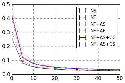
(a) PRE@K

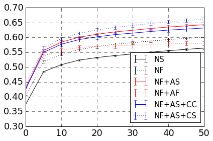
(b) REC@K

Figure 2. Performance of feature generation methods.

Method	avg. PRE	avg. REC	ACC
NS	$.03794\pm.00010$	$.5334\pm.0034$	$.6212\pm.0325$
NF	$.04553\pm.00018$	$.5708\pm.0052$	$.6718\pm.0107$
NF+AS	$.05216\pm.00030$	$.6162\pm.0067$	$.6917\pm.0181$
NF+AF	$.05008\pm.00018$	$.5866\pm.0061$	$.6424\pm.0324$
NF+AS+CC	$.05026\pm.00034$	$.6036\pm.0083$	$.6716\pm.0297$
NF+AS+CS	$.05508\pm.00024$	$.6476\pm.0058$	$.6989\pm.0135$

Table 1. Performance of feature generation methods.

Figure 2 and Table 1 show the performance of different feature generation methods. As can be clearly observed: 1) When we only consider the place name, NF performs significantly better than NS regarding all metrics, which supports our idea of training the advanced Fast-text model on the massive Facebook post corpus; 2) Incorporating place address is generally helpful, but the simple AS model we advocate for produces more significant improvements than the heavy AF model, which tells the importance of choosing the proper model rather than the complex one; 3) To leverage place coordinate and category, our proposed network-based embedding smoothing method (CS) is much more effective than the direct vector concatenation (CC).

The avg. PRE and avg. REC are taken over the 100 measures of PRE@$K$ and REC@$K$ when $K$ varies from 1 to 100, to directly compare and reveal the relative effectiveness of different methods. The absolute values of avg. PRE are pretty low because the numbers of labeled duplications are low in our testing data. Based on such results, we will use NF+AS+CS as our feature generation model and use its output $\mathcal{X}$ as the input of subsequent supervised metric learning models. Note that, other than places with the particular attributes as we focus on in this work, the methods developed here can be combined in different ways to capture textual, categorical and numerical attributes of various real-world objects.

6. Supervised Metric Learning

Besides place attributes, we also aim to leverage labeled place pairs through supervised metric learning. The idea is to learn a non-linear projection function $\mathcal{F}$, which transforms the place features $\mathcal{X}$ into a metric space, where duplicated places are close and non-duplicated places are far apart. Therefore, the model should be able to explore and stress the important features that indicate duplications.

6.1. Basic Models

We construct the basic metric learning models by applying simple MLP upon the place embedding $\mathcal{X}$. However, since direct leverage of standard triplet loss commonly used in person re-identification (Schroff et al., 2015) and entity resolution (Qu et al., 2017) in Eq. 1 requires the sampling of the third place based on our pair-wise place labels, which can introduce a lot of non-relevant and trivial training data, we propose to replace the triplet loss with a pair-wise contrastive loss as

$$\mathcal{J}_{pr}= \sum_{l=\{(a,b),y_{l}\}}[y_{l}d(\mathbf{u}_{a},\mathbf{u}_{b})+(1-y_{l})\text{ max}(0,\alpha-d(\mathbf{u}_{a},\mathbf{u}_{b}))],$$

where $d=d_{e}$ is the same as in Eq. 1. Besides the Euclidean distance function, we also tried various other distance functions including cosine similarity and learnable bilinear distance (Qu et al., 2017).

We comprehensively evaluated the performance of various basic models, and found that the PE (Pair-wise loss with Euclidean distance function) constantly performs the best, indicating the effectiveness of replacing the standard triplet loss in traditional CV and NLP tasks. Based on such observation, we will focus on further improving the PE model in the rest of this work.

6.2. Hard Sampling

Training the model with our massive noisy labeled place pairs can take quite significant time, most of which is wasted on trivial samples. To this end, we design the following novel criteria for dynamic batch-wise hard sampling towards our pair-wise loss.

$$C_{l=(a,b)} =\;\mathbb{I}\;[y_{l}d(\mathbf{u}_{a},\mathbf{u}_{b})-(1-y_{l})d(\mathbf{u}_{a},\mathbf{u}_{b})>$$

(3) $$\frac{\beta}{|B|}\sum_{l^{\prime}\in B}y_{l^{\prime}}d(\mathbf{u}_{a^{\prime}},\mathbf{u}_{b^{\prime}})-(1-y_{l^{\prime}})d(\mathbf{u}_{a^{\prime}},\mathbf{u}_{b^{\prime}})],$$

where $B$ denotes the set of samples in a batch, $\beta$ is the slack hyper-parameter controlling the amount of hard samples, and $d(\cdot)$ can be implemented with either $d_{f}(\cdot)$ or $d_{b}(\cdot)$. A sample pair $l$ is selected to contribute to the loss for gradient computation when $C_{l}=1$. The idea is to only focus on the hard samples where the model fails to put the labeled duplications close enough or non-duplications far away, compared with the average distances.

6.3. Attentive Training

Our labeled data are from different sources, which may have varying quality and bias. For example, data curated by a particular team at a certain time might be biased towards specific metrics. This often happens when people recognize the ignorance of particular situations and aim to improve them upon iterating to the next period of curation. Moreover, data labeled by the professional curation teams and rookie crowdsourcing workers can have quite different qualities. Therefore, it is intuitive to automatically assign different weights to the samples from different sources during training.

To deal with the varying quality and bias of training samples from multiple sources, we design a novel source-oriented attentive training technique based on the idea of self-attention (Denil et al., 2012; Vaswani et al., 2017), which has shown to be effective in various deep learning scenarios.

For each place $p_{i}$, rather than learning a single embedding vector $\mathbf{f}(\mathbf{x}_{i})$, we learn two embedding vectors $\mathbf{k}(\mathbf{x}_{i})$ and $\mathbf{v}(\mathbf{x}_{i})$, which we call the key embedding and value embedding, respectively. In practice, we can implement both $\mathbf{k}(\cdot)$ and $\mathbf{v}(\cdot)$ as FNNs and let them share a few layers. Besides, we also learn a global source embedding $\mathbf{q}(s_{j})$ for each training source $s_{j}$, which can be implemented as an embedding look-up table. The size of $\mathbf{q}(\cdot)$ is twice as $\mathbf{k}(\cdot)$. Subsequently, we design the weight of the training sample $l=(a,b)$ from source $s$ as

(4) $$w_{ls}=\frac{\exp([\mathbf{k}(\mathbf{x}_{a}),\mathbf{k}(\mathbf{x}_{b})]^{T}\mathbf{q}(s))}{\sum_{s^{\prime}}\exp([\mathbf{k}(\mathbf{x}_{a}),\mathbf{k}(\mathbf{x}_{b})]^{T}\mathbf{q}(s^{\prime}))},$$

where $[\cdot]$ denotes vector concatenation. With $\mathcal{W}$ defined, we rewrite our loss function in Eq. 6.1 into

$$\mathcal{J}_{pr}^{\prime}= \sum_{s}\sum_{l=\{(a,b),y_{l}\}\in\mathcal{T}_{s}}w_{ls}[y_{l}d(\mathbf{v}(\mathbf{x}_{a}),\mathbf{v}(\mathbf{x}_{b}))$$

(5) $$+(1-y_{l})\text{ max}(0,\alpha-d(\mathbf{v}(\mathbf{x}_{a}),\mathbf{v}(\mathbf{x}_{b})))],$$

where $\mathcal{T}_{s}$ denotes the set of training samples from source $s$.

Training with Eq. 5 allows the model to learn a source-oriented self-attention weight for each training pair. To be specific, if similar samples keep appearing in a certain source, they are likely redundant and less useful, and the model will automatically reduce their contribution to the loss. However, if similar samples appear across different sources, the model will put more trust on their correctness by relatively increasing their attention weights. Finally, unseen samples will likely get higher attention.

6.4. Label Denoising

Place deduplication can be essentially regarded as a semi-supervised clustering problem, where pages of the same places should naturally form clusters in the embedding space. This is true mainly because the duplication relationship is transitive. While such clusters are ideal for duplication detection, they can also help reduce the noise within training data, i.e., labels that conflict with the cluster structures are likely noisy. To leverage this insight, we design a novel soft clustering-based label denoising module based on the idea of self-training neural networks (Nigam and Ghani, 2000; Xie et al., 2016; Guo et al., 2017). Particularly, we introduce a loss based on the KL-divergence

(6) $$\mathcal{J}_{dn}=\rho\;\text{KL}(\mathcal{C}||\mathcal{D})=\rho\sum_{i}\sum_{k}c_{ik}\log\frac{c_{ik}}{d_{ik}},$$

where $\rho$ is a hyper-parameter. $d_{ik}\in\mathcal{D}$ is the probability of assigning place $p_{i}$ to the $k$th cluster, under the assumption of Student’s $t$-distribution with degree of freedom set to 1 (Maaten and Hinton, 2008), i.e.,

(7) $$d_{ik}=\frac{(1+||\mathbf{f}(\mathbf{x}_{i})-\mathbf{u}_{k}||^{2})^{-1}}{\sum_{j}(1+||\mathbf{f}(\mathbf{x}_{i})-\mathbf{u}_{j}||^{2})^{-1}}.$$

It is basically a kernel function that measures the similarity between the embedding of place $p_{i}$ and the cluster center $u_{k}$. $\mathcal{C}$ is an auxiliary target distribution defined as

(8) $$c_{ik}=\frac{d_{ik}^{2}/g_{k}}{\sum_{k^{\prime}}d_{ik^{\prime}}^{2}/g_{k^{\prime}}},$$

where $g_{k}=\sum_{i}d_{ik}$ is the total number of places softly assigned to the $k$th cluster. Raising $\mathcal{D}$ to the second power and then dividing by the number of places per cluster allows the target distribution $\mathcal{C}$ to improve cluster purity and leverage the confident assignments to help reduce the influence of noisy labels.

6.5. Experimental Evaluations

We compare the following methods to demonstrate the effectiveness of our proposed supervised metric learning techniques.

• NF+AS+CS: The best place features we got through unsupervised feature generation in Section 5, which is also the input of the following metric learning methods.

• PE: The best basic metric learning method adapted from CV and NLP with the Pair-wise contrastive loss and Euclidean distance function, as discussed in Section 6.1.

• PEH: PE improved with batch-wise hard sampling.

• PEHA: PEH improved with our novel source-oriented attentive training technique.

• PEHAD: PEHA improved with our novel soft clustering-based label denoising technique.

We also compare our models with several state-of-the-art classification algorithms that can be applied for pair-wise duplication prediction, i.e., logistic regression (LR), support vector machine (SVM), random forest (RF) and gradient boosting decision tree (GBDT). These algorithms do not produce place embeddings and thus cannot be efficiently evaluated through fast $k$-NN in datasets with hundreds of millions of places. Therefore, we only compute their standard classification accuracy of duplication prediction on the testing data, as shown in Table 2.

Method	LR	SVM	RF	GBDT	PEHAD
ACC	$0.7514$	$0.7699$	$0.7786$	$0.7828$	$0.9279$

Table 2. Performance of state-of-the-art algorithms.

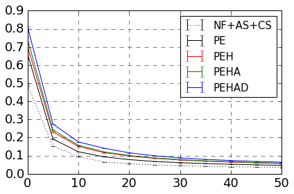
(a) PRE@K

(b) REC@K

Figure 3. Performance of our metric learning methods.

Method	avg. PRE	avg. REC	ACC
NF+AS+CS	$.05508\pm.00024$	$.6476\pm.0058$	$.6989\pm.0135$
PE	$.07533\pm.00034$	$.7534\pm.0083$	$.7926\pm.0297$
PEH	$.08970\pm.00039$	$.8434\pm.0102$	$.8580\pm.0238$
PEHA	$.09274\pm.00019$	$.8554\pm.0047$	$.8815\pm.0100$
PEHAD	$.10780\pm.00021$	$.9119\pm.0062$	$.9279\pm.0104$

Table 3. Performance of our metric learning methods.

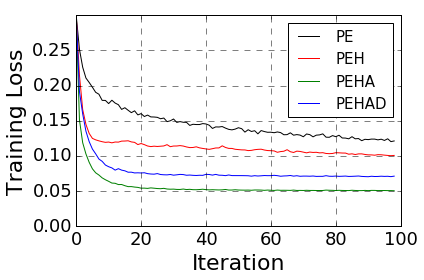
(a) Training loss

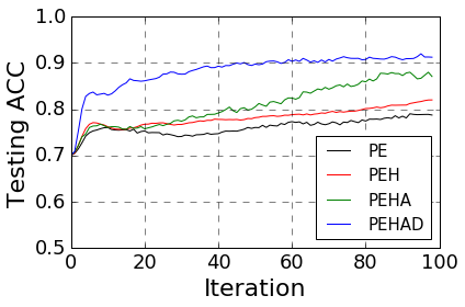
(b) Testing accuracy

Figure 4. Training loss and testing accuracy curves.

Figure 3 and Table 3 show the performance of compared models. As we can see, our supervised metric learning framework can significantly improve the place embedding quality, because labeled data allow the models to pick out the more important features that differentiate duplication pairs from non-duplications. Moreover, each of our proposed model components further boosts the overall model performance, and their coherent combination (PEHAD) has the best performance regarding all metrics in the evaluation. Our models also significantly outperform all of the state-of-the-art non-embedding algorithms in Table 2– PEHAD achieves over 18% relative improvement on GBDT (the strongest baseline).

To better understand how each of the components contributes to the overall model, we also closely observe the training loss and testing accuracy during the training of different models. As we can see in Figure 4: 1) Hard sampling is effective in speeding up the convergence of training loss, and allows the model to keep learning after the loss seems to converge; 2) Attentive training leads to lower losses due to the additional weights. It does not lead to significant performance gain on top of the basic PE model with hard sampling, but it does make the training process more stable and reduce the performance variance across different trains of the same model; 3) Label denoising empowers the model to rapidly remove the influence of noisy labels and achieve the peak performance after a small number of training iterations, which may further allow efficient model training with early stop.

Finally, all techniques here are also not bounded to the problem of place deduplication, but can rather be combined to leverage noisy pair-wise labels from multiple sources in various other domains.

7. Conclusions

In this paper, we collect data from the real-world place graph of Facebook as an example to systematically study the novel problem of place deduplication and comprehensively evaluate the effectiveness of our proposed place embedding pipeline. The concepts and methods developed, although do not provide an end-solution for place deduplication, successfully improve the quality of place embedding for intermediate tasks like duplication prediction and candidate fetch, which largely facilitates further place deduplication.

As for future work, it is interesting to further improve both the unsupervised feature generation model to incorporate more attributes, and the supervised metric learning model to leverage various training signals with efficiency. It is also interesting to apply the learned place embedding to facilitate other tasks related to place graph quality such as junk place prediction and common place clustering, as well as downstream applications including next destination recommendation and location-based ads ranking.

References

- (1)
- Bojanowski et al. (2017) Piotr Bojanowski, Edouard Grave, Armand Joulin, and Tomas Mikolov. 2017. Enriching word vectors with subword information. TACL (2017).
- Chakrabarti et al. (2012) Kaushik Chakrabarti, Surajit Chaudhuri, Tao Cheng, and Dong Xin. 2012. A framework for robust discovery of entity synonyms. In KDD. ACM, 1384–1392.
- Chen et al. (2018) Haolan Chen, Fred X Han, Di Niu, Dong Liu, Kunfeng Lai, Chenglin Wu, and Yu Xu. 2018. MIX: Multi-Channel Information Crossing for Text Matching. In KDD. ACM, 110–119.
- Chen et al. (2016) Shi-Zhe Chen, Chun-Chao Guo, and Jian-Huang Lai. 2016. Deep ranking for person re-identification via joint representation learning. TIP 25, 5 (2016), 2353–2367.
- Chen et al. (2017) Weihua Chen, Xiaotang Chen, Jianguo Zhang, and Kaiqi Huang. 2017. Beyond triplet loss: a deep quadruplet network for person re-identification. In CVPR, Vol. 2. IEEE.
- Cheng et al. (2016) De Cheng, Yihong Gong, Sanping Zhou, Jinjun Wang, and Nanning Zheng. 2016. Person re-identification by multi-channel parts-based cnn with improved triplet loss function. In CVPR. IEEE, 1335–1344.
- Christen et al. (2015) Peter Christen, Dinusha Vatsalan, and Qing Wang. 2015. Efficient entity resolution with adaptive and interactive training data selection. In ICDM. IEEE, 727–732.
- Chuang and Chang (2015) Hsiu-Min Chuang and Chia-Hui Chang. 2015. Verification of poi and location pairs via weakly labeled web data. In WWW. ACM, 743–748.
- Dal Bianco et al. (2016) Guilherme Dal Bianco, Renata Galante, Carlos A Heuser, Marcos Gonçalves, and Sergio Canuto. 2016. A practical and effective sampling selection strategy for large scale deduplication. In ICDE. IEEE, 1518–1519.
- Dalvi et al. (2014) Nilesh Dalvi, Marian Olteanu, Manish Raghavan, and Philip Bohannon. 2014. Deduplicating a places database. In WWW. ACM, 409–418.
- Denil et al. (2012) Misha Denil, Loris Bazzani, Hugo Larochelle, and Nando de Freitas. 2012. Learning where to attend with deep architectures for image tracking. Neural computation 24, 8 (2012), 2151–2184.
- Ding et al. (2015) Shengyong Ding, Liang Lin, Guangrun Wang, and Hongyang Chao. 2015. Deep feature learning with relative distance comparison for person re-identification. Pattern Recognition 48, 10 (2015), 2993–3003.
- Ference et al. (2013) Gregory Ference, Mao Ye, and Wang-Chien Lee. 2013. Location recommendation for out-of-town users in location-based social networks. In CIKM. ACM, 721–726.
- Garcia et al. (2008) Vincent Garcia, Eric Debreuve, and Michel Barlaud. 2008. Fast k nearest neighbor search using GPU. In CVPRW. IEEE, 1–6.
- Guo et al. (2016) Jiafeng Guo, Yixing Fan, Qingyao Ai, and W Bruce Croft. 2016. A deep relevance matching model for ad-hoc retrieval. In CIKM. ACM, 55–64.
- Guo et al. (2017) Xifeng Guo, Long Gao, Xinwang Liu, and Jianping Yin. 2017. Improved Deep Embedded Clustering with Local Structure Preservation. In IJCAI.
- Han et al. (2011) Jiawei Han, Jian Pei, and Micheline Kamber. 2011. Data mining: concepts and techniques. Elsevier.
- He et al. (2016) Yeye He, Kaushik Chakrabarti, Tao Cheng, and Tomasz Tylenda. 2016. Automatic discovery of attribute synonyms using query logs and table corpora. In WWW. ACM, 1429–1439.
- Hu et al. (2014) Baotian Hu, Zhengdong Lu, Hang Li, and Qingcai Chen. 2014. Convolutional neural network architectures for matching natural language sentences. In NIPS. 2042–2050.
- Johnson et al. (2017) Jeff Johnson, Matthijs Douze, and Hervé Jégou. 2017. Billion-scale similarity search with GPUs. arXiv preprint arXiv:1702.08734 (2017).
- Joulin et al. (2017) Armand Joulin, Edouard Grave, Piotr Bojanowski, and Tomas Mikolov. 2017. Bag of Tricks for Efficient Text Classification. In EACL, Vol. 2. 427–431.
- Kozhevnikov and Gorovoy (2016) Ivan Kozhevnikov and Vladimir Gorovoy. 2016. Comparison of Different Approaches for Hotels Deduplication. In KESW. Springer, 230–240.
- Li et al. (2015) Xutao Li, Gao Cong, Xiao-Li Li, Tuan-Anh Nguyen Pham, and Shonali Krishnaswamy. 2015. Rank-geofm: A ranking based geographical factorization method for point of interest recommendation. In SIGIR. ACM, 433–442.
- Lian et al. (2014) Defu Lian, Cong Zhao, Xing Xie, Guangzhong Sun, Enhong Chen, and Yong Rui. 2014. GeoMF: joint geographical modeling and matrix factorization for point-of-interest recommendation. In KDD. ACM, 831–840.
- Liu et al. (2014) Yong Liu, Wei Wei, Aixin Sun, and Chunyan Miao. 2014. Exploiting geographical neighborhood characteristics for location recommendation. In CIKM. 739–748.
- Maaten and Hinton (2008) Laurens van der Maaten and Geoffrey Hinton. 2008. Visualizing data using t-SNE. JMLR 9, Nov (2008), 2579–2605.
- Mikolov et al. (2018) Tomas Mikolov, Edouard Grave, Piotr Bojanowski, Christian Puhrsch, and Armand Joulin. 2018. Advances in pre-training distributed word representations. In LREC.
- Mikolov et al. (2013) Tomas Mikolov, Ilya Sutskever, Kai Chen, Greg S Corrado, and Jeff Dean. 2013. Distributed representations of words and phrases and their compositionality. In NIPS. 3111–3119.
- Nigam and Ghani (2000) Kamal Nigam and Rayid Ghani. 2000. Analyzing the effectiveness and applicability of co-training. In CIKM. ACM, 86–93.
- Pang et al. (2016) Liang Pang, Yanyan Lan, Jiafeng Guo, Jun Xu, Shengxian Wan, and Xueqi Cheng. 2016. Text Matching as Image Recognition.. In AAAI. 2793–2799.
- Qian et al. (2017) Kun Qian, Lucian Popa, and Prithviraj Sen. 2017. Active Learning for Large-Scale Entity Resolution. In CIKM. ACM, 1379–1388.
- Qian et al. (2009) Longhua Qian, Guodong Zhou, Fang Kong, and Qiaoming Zhu. 2009. Semi-supervised learning for semantic relation classification using stratified sampling strategy. In EMNLP. 1437–1445.
- Qu et al. (2017) Meng Qu, Xiang Ren, and Jiawei Han. 2017. Automatic Synonym Discovery with Knowledge Bases. In KDD. ACM, 997–1005.
- Ren and Cheng (2015) Xiang Ren and Tao Cheng. 2015. Synonym discovery for structured entities on heterogeneous graphs. In WWW. ACM, 443–453.
- Roller et al. (2014) Stephen Roller, Katrin Erk, and Gemma Boleda. 2014. Inclusive yet selective: Supervised distributional hypernymy detection. In COLING. 1025–1036.
- Sarwat et al. (2014) Mohamed Sarwat, Justin J Levandoski, Ahmed Eldawy, and Mohamed F Mokbel. 2014. LARS*: An efficient and scalable location-aware recommender system. TKDE 26, 6 (2014), 1384–1399.
- Schroff et al. (2015) Florian Schroff, Dmitry Kalenichenko, and James Philbin. 2015. Facenet: A unified embedding for face recognition and clustering. In CVPR. IEEE, 815–823.
- Su et al. (2016) Chi Su, Shiliang Zhang, Junliang Xing, Wen Gao, and Qi Tian. 2016. Deep attributes driven multi-camera person re-identification. In ECCV. 475–491.
- Sun and Grishman (2010) Ang Sun and Ralph Grishman. 2010. Semi-supervised semantic pattern discovery with guidance from unsupervised pattern clusters. In COLING. 1194–1202.
- Sun and Wu (2018) Qiang Sun and Yue Wu. 2018. A Multi-level Attention Model for Text Matching. In ICANN. Springer, 142–153.
- Sun et al. (2015) Yi Sun, Xiaogang Wang, and Xiaoou Tang. 2015. Deeply learned face representations are sparse, selective, and robust. In CVPR. IEEE, 2892–2900.
- Taigman et al. (2014) Yaniv Taigman, Ming Yang, Marc’Aurelio Ranzato, and Lior Wolf. 2014. Deepface: Closing the gap to human-level performance in face verification. In CVPR. 1701–1708.
- Ustalov et al. (2017) Dmitry Ustalov, Alexander Panchenko, and Chris Biemann. 2017. Watset: automatic induction of synsets from a graph of synonyms. In ACL.
- Vaswani et al. (2017) Ashish Vaswani, Noam Shazeer, Niki Parmar, Jakob Uszkoreit, Llion Jones, Aidan N Gomez, Łukasz Kaiser, and Illia Polosukhin. 2017. Attention is all you need. In NIPS. 5998–6008.
- Wan et al. (2016) Shengxian Wan, Yanyan Lan, Jiafeng Guo, Jun Xu, Liang Pang, and Xueqi Cheng. 2016. A Deep Architecture for Semantic Matching with Multiple Positional Sentence Representations.. In AAAI, Vol. 16. 2835–2841.
- Wang et al. (2016) Faqiang Wang, Wangmeng Zuo, Liang Lin, David Zhang, and Lei Zhang. 2016. Joint learning of single-image and cross-image representations for person re-identification. In CVPR. IEEE, 1288–1296.
- Weeds et al. (2014) Julie Weeds, Daoud Clarke, Jeremy Reffin, David Weir, and Bill Keller. 2014. Learning to distinguish hypernyms and co-hyponyms. In COLING. 2249–2259.
- Xie et al. (2016) Junyuan Xie, Ross Girshick, and Ali Farhadi. 2016. Unsupervised deep embedding for clustering analysis. In ICML. IEEE, 478–487.
- Xiong et al. (2017) Chenyan Xiong, Zhuyun Dai, Jamie Callan, Zhiyuan Liu, and Russell Power. 2017. End-to-end neural ad-hoc ranking with kernel pooling. In SIGIR. ACM, 55–64.
- Yang et al. (2017) Carl Yang, Lanxiao Bai, Chao Zhang, Quan Yuan, and Jiawei Han. 2017. Bridging collaborative filtering and semi-supervised learning: a neural approach for poi recommendation. In KDD. ACM, 1245–1254.
- Yang et al. (2018) Carl Yang, Chao Zhang, Xuewen Chen, Jieping Ye, and Jiawei Han. 2018. Did You Enjoy the Ride: Understanding Passenger Experience via Heterogeneous Network Embedding. In ICDE.
- Ye et al. (2011) Mao Ye, Peifeng Yin, Wang-Chien Lee, and Dik-Lun Lee. 2011. Exploiting geographical influence for collaborative point-of-interest recommendation. In SIGIR. ACM, 325–334.
- Yin et al. (2015) Hongzhi Yin, Xiaofang Zhou, Yingxia Shao, Hao Wang, and Shazia Sadiq. 2015. Joint modeling of user check-in behaviors for point-of-interest recommendation. In CIKM. ACM, 1631–1640.