Learning interaction kernels in heterogeneous systems of agents from multiple trajectories

\nameFei Lu1,3 \emailfeilu@math.jhu.edu
\AND\nameMauro Maggioni1,2,3 \emailmauromaggionijhu@icloud.com
\AND\nameSui Tang1,4 \emailsuitang@math.ucsb.edu
\addr1Departments of Mathematics, 2Applied Mathematics and Statistics,
3Johns Hopkins University, 3400 N. Charles Street, Baltimore, MD 21218, USA
4University of California, Santa Barbara, 552 University Rd, Isla Vista, CA 93117, USA
Abstract

Systems of interacting particles or agents have wide applications in many disciplines such as Physics, Chemistry, Biology and Economics. These systems are governed by interaction laws, which are often unknown: estimating them from observation data is a fundamental task that can provide meaningful insights and accurate predictions of the behaviour of the agents. In this paper, we consider the inverse problem of learning interaction laws given data from multiple trajectories, in a nonparametric fashion, when the interaction kernels depend on pairwise distances. We establish a condition for learnability of interaction kernels, and construct estimators that are guaranteed to converge in a suitable L2superscript𝐿2L^{2} space, at the optimal min-max rate for 1-dimensional nonparametric regression. We propose an efficient learning algorithm based on least squares, which can be implemented in parallel for multiple trajectories and is therefore well-suited for the high dimensional, big data regime. Numerical simulations on a variety examples, including opinion dynamics, predator-swarm dynamics and heterogeneous particle dynamics, suggest that the learnability condition is satisfied in models used in practice, and the rate of convergence of our estimator is consistent with the theory. These simulations also suggest that our estimators are robust to noise in the observations, and produce accurate predictions of dynamics in relative large time intervals, even when they are learned from data collected in short time intervals.

Keywords: Interacting particle systems; inverse problems; Monte Carlo sampling; regularized least squares; nonparametric statistics.


Acknowledgments

FL and MM are grateful for partial support from NSF-1913243, FL for NSF-1821211; MM for NSF-1837991, NSF-1546392 and AFOSR-FA9550-17-1-0280; ST for NSF-1546392 and AFOSR-FA9550-17-1-0280 and AMS Simons travel grant.


1 Introduction

Systems of interacting particles and agents arise in a wide variety of disciplines including interacting particle systems in Physics (see D’Orsogna et al. (2006); Vicsek et al. (1995); Chuang et al. (2007); Bellomo et al. (2017)), predator-swarm systems in Biology (see Hemelrijk and Hildenbrandt (2011); Toner and Tu (1995)) , and opinions on interacting networks in social science (see Olfati-Saber and Murray (2004); Mostch and Tadmor (2014); Ke et al. (2002)). The interacting system is often modeled by a system of ODEs where the form of the equations is given and the unknowns are the interaction kernels. Inference of these kernels is useful for modeling and predictions, yet it is a fundamental challenge. In the past, due to the limited amount of data, the estimation of interaction kernels often relied on strong a priori assumptions, which reduced the estimate to a small number of parameters within a given family of possible kernels. With the increased collection and availability of data, computational power, and data storage, it is expected to enable the automatic discovery of interaction laws from data, under minimal assumptions on the form of such laws. We consider the following inverse problem: given trajectory data of a particle/agent system, collected from different experiment trials, how to discover the interaction law? We use tools from statistical and machine learning to propose a learning algorithm guided by rigorous analysis to estimate the interaction kernels, and accurately predict the dynamics of the system using the estimated interaction kernels.

Many governing laws of complex dynamical processes are presented in the form of (ordinary or partial) differential equations. The problem of learning differential equations from data, including those arising from systems of interacting agents, has attracted continuous attention of researchers from various disciplines. Pioneering work of learning interaction kernels in system of interacting agents can be found in the work of Lukeman et al. (2010); Katz et al. (2011); Wang et al. (2018), where the true kernels are assumed to lie in the span of a predetermined set of template functions and parametric regression techniques are used to recover the kernels either from real (see Lukeman et al. (2010); Katz et al. (2011)) or the synthetic (see Wang et al. (2018)) trajectory data. In Bongini et al. (2017), the authors considered learning interaction kernels from data collected from a single trajectory in a nonparametric fashion and a recovery guarantee is proved when the number of agents goes to infinity. For nonlinear coupled dynamical systems, symbolic regression techniques are employed to reveal governing laws in various systems from experiment trajectory data sets without any prior knowledge about the underlying dynamics (see Bongard and Lipson (2007); Schmidt and Lipson (2009)). Recently, the problem of learning high dimensional nonlinear differential equations from the synthetic trajectory data, where the dynamics are governed by a few numbers of active terms in a prescribed large dictionary, has raised a lot of attention. Sparse regression approaches include SINDy (Brunton et al. (2016); Rudy et al. (2017); Brunton et al. (2017); Boninsegna et al. (2018)), LASSO (Schaeffer et al. (2013); Han et al. (2015); Kang et al. (2019)), threshold sparse Bayesian regression (Zhang and Lin (2018)), have been shown to enable effective identification of the activate terms from the trajectory data sets. Recovery guarantees are established under suitable assumptions on the noise in the observation and randomness of data (Tran and Ward (2017); Schaeffer et al. (2018)). There are also approaches using deep learning techniques to learn ODEs (see Raissi et al. (2018); Rudy et al. (2019)) and PDEs (see Raissi (2018); Raissi and Karniadakis (2018); Long et al. (2017)) from the synthetic trajectory/solution data sets. These techniques make use of approximation power of the deep neural network to construct estimators for response operators and have shown superior empirical performance. In the Statistics community, parameter estimation for differential equations from trajectory data has been studied in Varah (1982); Brunel (2008); Liang and Wu (2008); Cao et al. (2011); Ramsay et al. (2007), among others, and references therein. The form of the differential equations is given, and the unknown is a parameter 𝜽𝜽\boldsymbol{\theta} in Euclidean space. Approaches include the trajectory matching method, that chooses 𝜽𝜽\boldsymbol{\theta} so as to maximize agreement with the trajectory data, the gradient matching method that seeks 𝜽𝜽\boldsymbol{\theta} to fit the right-hand side of the ODEs to the velocities of the trajectory data, and the parameter cascading method that combines the virtues of previous two methods, but avoids the heavy computational overhead of trajectory matching method and is applicable to partial/indirect observations which the gradient matching method currently can not handle. A review of the parameter estimation problem in system of ODEs may be found in Ramsay and Hooker (2018). The identifiability of 𝜽𝜽\boldsymbol{\theta} in general systems of nonlinear ODEs from trajectory data is challenging and a topic of current research. It is often assumed that the parameters are identifiable from the trajectory data, i.e, different 𝜽𝜽\boldsymbol{\theta} would yield different trajectories during the observation period. There is no easy way to check this assumption from data, and characterizations of identifiability exist for some special cases (e.g., see Dattner and Klaassen (2015) for systems of ordinary differential equations with a linear dependence on (known functions of) the parameters. We refer the interested reader to Miao et al. (2011) and references therein for a comprehensive survey of this topic.

In this paper, we restrict our attention to learning governing laws in first order particle-/agent-based systems with pairwise interactions, whose magnitudes only depend on mutual distances. We consider an N𝑁N-agent system with K𝐾K types of agents in the Euclidean space dsuperscript𝑑\mathbb{R}^{d} and denote by {Ck}k=1Ksuperscriptsubscriptsubscript𝐶𝑘𝑘1𝐾\{C_{k}\}_{k=1}^{K} the partition of the set of indices {1,,N}1𝑁\{1,\dots,N\} of the agents corresponding to their type. Suppose there are different interaction kernels for each ordered pair of types and that the agents evolve according to the system of ODEs :

𝒙˙i(t)subscript˙𝒙𝑖𝑡\displaystyle\dot{\boldsymbol{x}}_{i}(t) =i=1N1N𝓀𝒾ϕ𝓀𝒾𝓀𝒾(𝒙i(t)𝒙i(t))(𝒙i(t)𝒙i(t)),i=1,,N.formulae-sequenceabsentsuperscriptsubscriptsuperscript𝑖1𝑁1subscript𝑁subscript𝓀superscript𝒾subscriptitalic-ϕsubscript𝓀𝒾subscript𝓀superscript𝒾normsubscript𝒙superscript𝑖𝑡subscript𝒙𝑖𝑡subscript𝒙superscript𝑖𝑡subscript𝒙𝑖𝑡𝑖1𝑁\displaystyle=\sum_{i^{\prime}=1}^{N}\frac{1}{N_{\mathpzc{k}_{i^{\prime}}}}\phi_{\mathpzc{k}_{i}\mathpzc{k}_{i^{\prime}}}(||\boldsymbol{x}_{i^{\prime}}(t)-\boldsymbol{x}_{i}(t)||)(\boldsymbol{x}_{i^{\prime}}(t)-\boldsymbol{x}_{i}(t))\,,i=1,\cdots,N\,. (1.1)

where 𝒙˙i(t):=ddt𝒙i(t)assignsubscript˙𝒙𝑖𝑡𝑑𝑑𝑡subscript𝒙𝑖𝑡\dot{\boldsymbol{x}}_{i}(t):=\frac{d}{dt}\boldsymbol{x}_{i}(t);𝓀𝒾subscript𝓀𝒾\mathpzc{k}_{i} is the index of the type of agent i𝑖i, i.e. iC𝓀𝒾𝑖subscript𝐶subscript𝓀𝒾i\in C_{\mathpzc{k}_{i}}; N𝓀𝒾subscript𝑁subscript𝓀superscript𝒾N_{\mathpzc{k}_{i^{\prime}}} is the number of agents of type C𝓀𝒾subscript𝐶subscript𝓀superscript𝒾C_{\mathpzc{k}_{i^{\prime}}}. The interaction kernel ϕ𝓀𝒾𝓀𝒾:+\phi_{\mathpzc{k}_{i}\mathpzc{k}_{i^{\prime}}}:_{+}\rightarrow governs how agents in type C𝓀𝒾subscript𝐶subscript𝓀𝒾C_{\mathpzc{k}_{i}} influence agents in type C𝓀𝒾subscript𝐶subscript𝓀superscript𝒾C_{\mathpzc{k}_{i^{\prime}}}. In this system, the velocity of each agent is obtained by superimposing the interactions with all the other agents, with each interaction being in the direction to the other agent, weighted by the interaction kernel evaluated at the distance to the other agent. We will let rii:=𝒙i𝒙iassignsubscript𝑟𝑖superscript𝑖normsubscript𝒙superscript𝑖subscript𝒙𝑖r_{ii^{\prime}}:=\left\|\boldsymbol{x}_{i^{\prime}}-\boldsymbol{x}_{i}\right\|, 𝒓ii:=𝒙i𝒙iassignsubscript𝒓𝑖superscript𝑖subscript𝒙superscript𝑖subscript𝒙𝑖\boldsymbol{r}_{ii^{\prime}}:=\boldsymbol{x}_{i^{\prime}}-\boldsymbol{x}_{i}. We assume that the interaction kernels ϕ𝓀𝒾𝓀𝒾subscriptitalic-ϕsubscript𝓀𝒾subscript𝓀superscript𝒾\smash{\phi_{\mathpzc{k}_{i}\mathpzc{k}_{i^{\prime}}}} are the only unknown factors in (1.1); in particular, the sets Cksubscript𝐶𝑘C_{k}’s are pre-specified. Below we summarize the notation used in first order models.

Variable Definition
𝒙i(t)dsuperscript𝑑subscript𝒙𝑖𝑡absent\boldsymbol{x}_{i}(t)\in^{d} state vector (position, opinion, etc.) of agent i𝑖i at time t𝑡t
\|\cdot\| Euclidean norm in dsuperscript𝑑\mathbb{R}^{d}
𝒓ii(t),𝒓ii′′(t)dsuperscript𝑑subscript𝒓𝑖superscript𝑖𝑡subscript𝒓𝑖superscript𝑖′′𝑡absent\boldsymbol{r}_{ii^{\prime}}(t),\boldsymbol{r}_{ii^{\prime\prime}}(t)\in^{d} 𝒙i(t)𝒙i(t)subscript𝒙superscript𝑖𝑡subscript𝒙𝑖𝑡\boldsymbol{x}_{i^{\prime}}(t)-\boldsymbol{x}_{i}(t), 𝒙i′′(t)𝒙i(t)subscript𝒙superscript𝑖′′𝑡subscript𝒙𝑖𝑡\boldsymbol{x}_{i^{\prime\prime}}(t)-\boldsymbol{x}_{i}(t)
rii(t),rii′′(t)+superscriptsubscript𝑟𝑖superscript𝑖𝑡subscript𝑟𝑖superscript𝑖′′𝑡absentr_{ii^{\prime}}(t),r_{ii^{\prime\prime}}(t)\in^{+} rii(t)=𝒓ii(t),rii′′(t)=𝒓ii(t)formulae-sequencesubscript𝑟𝑖superscript𝑖𝑡normsubscript𝒓𝑖superscript𝑖𝑡subscript𝑟𝑖superscript𝑖′′𝑡normsubscript𝒓𝑖superscript𝑖𝑡r_{ii^{\prime}}(t)=\|\boldsymbol{r}_{ii^{\prime}}(t)\|,r_{ii^{\prime\prime}}(t)=\|\boldsymbol{r}_{ii^{\prime}}(t)\|
N𝑁N number of agents
K𝐾K number of types
Nksubscript𝑁𝑘N_{k} number of agents in type k𝑘k
𝓀𝒾subscript𝓀𝒾\mathpzc{k}_{i} type of agent i𝑖i
Cksubscript𝐶𝑘C_{k} the set of indices of the agents of type k𝑘k
ϕkksubscriptitalic-ϕ𝑘superscript𝑘\phi_{kk^{\prime}} interaction kernel for the influence of agents of type k𝑘k on agents of type ksuperscript𝑘k^{\prime}
Table 1: Notation for first-order models

We let 𝑿(t):=(𝒙i(t))i=1Nassign𝑿𝑡superscriptsubscriptsubscript𝒙𝑖𝑡𝑖1𝑁\boldsymbol{X}(t):=(\boldsymbol{x}_{i}(t))_{i=1}^{N} in the state space dN be the vector describing the state of the system; we let ϕ:=(ϕkk)k,k=1K,Kassignbold-italic-ϕsuperscriptsubscriptsubscriptitalic-ϕ𝑘superscript𝑘𝑘superscript𝑘1𝐾𝐾{\bm{\phi}}:=(\phi_{kk^{\prime}})_{k,k^{\prime}=1}^{K,K} denote the interaction kernels, and 𝐟ϕ(𝑿)dNsuperscript𝑑𝑁subscript𝐟bold-italic-ϕ𝑿absent\mathbf{f}_{{\bm{\phi}}}(\boldsymbol{X})\in^{dN} be the vectorization of the right hand side of (1.1). We can then rewrite the equations in (1.1) as

𝑿˙(t)=𝐟ϕ(𝑿(t)).˙𝑿𝑡subscript𝐟bold-italic-ϕ𝑿𝑡\displaystyle\dot{\boldsymbol{X}}(t)=\mathbf{f}_{{\bm{\phi}}}(\boldsymbol{X}(t)). (1.2)

The observational data 𝑿traj,M,μ0:={𝑿(m)(tl),𝑿˙(m)(tl)}l,m=1,1L,Massignsubscript𝑿traj𝑀subscript𝜇0superscriptsubscriptsuperscript𝑿𝑚subscript𝑡𝑙superscript˙𝑿𝑚subscript𝑡𝑙formulae-sequence𝑙𝑚11𝐿𝑀\boldsymbol{X}_{\text{traj},M,\mu_{0}}:=\{\boldsymbol{X}^{(m)}(t_{l}),\dot{\boldsymbol{X}}^{(m)}(t_{l})\}_{l,m=1,1}^{L,M} consist of the positions and velocities of all agents observed at time 0=t1<<tL=T0subscript𝑡1subscript𝑡𝐿𝑇0=t_{1}<\dots<t_{L}=T; m𝑚m indexes trajectories corresponding to different initial conditions {𝑿(m)(0)}m=1Msuperscriptsubscriptsuperscript𝑿𝑚0𝑚1𝑀\{\boldsymbol{X}^{(m)}(0)\}_{m=1}^{M}, which are assumed sampled i.i.d from a probability measure μ0subscript𝜇0\mu_{0} on the state space dNsuperscript𝑑𝑁\mathbb{R}^{dN}. We will consider the case where the times tlsubscript𝑡𝑙t_{l} are equi-spaced, but minor and straightforward modifications would yield the general case.

The goal is to learn the interaction kernels (ϕkk)k,k=1,1K,Ksuperscriptsubscriptsubscriptitalic-ϕ𝑘superscript𝑘formulae-sequence𝑘superscript𝑘11𝐾𝐾(\phi_{kk^{\prime}})_{k,k^{\prime}=1,1}^{K,K} from 𝑿traj,M,μ0subscript𝑿traj𝑀subscript𝜇0\boldsymbol{X}_{\text{traj},M,\mu_{0}} and predict the dynamics given a new initial condition drawn from μ0subscript𝜇0\mu_{0}. The case of K=1𝐾1K=1 and M=1𝑀1M=1 has been considered in Bongini et al. (2017) in the mean field regime (N)𝑁(N\rightarrow\infty); here we consider the case when the number of agents N𝑁N is fixed and the number of observed trajectories M𝑀M is large, and the more general case of multi-type agents (for some instances of which the mean-field theory is fraught with difficulties). In summary, we consider the regime where L𝐿L fixed, and M𝑀M\rightarrow\infty. No ergodicity requirement on the dynamical system is needed.

Inspired by the work in Bongini et al. (2017), we introduced a risk functional in our recent work Lu et al. (2019) that exploits the structure of the system (1.1), and minimize it over a hypothesis function class 𝓗Msubscript𝓗𝑀\boldsymbol{\mathcal{H}}_{M}, to obtain estimators of the true kernels ϕbold-italic-ϕ{\bm{\phi}}:

𝓔M(𝝋)::subscript𝓔𝑀𝝋absent\displaystyle\boldsymbol{\mathcal{E}}_{M}({\bm{\varphi}}): =1MLm=1,l=1M,L𝑿˙(m)(tl)𝐟𝝋(𝑿(m)(tl))𝒮2,absent1𝑀𝐿superscriptsubscriptformulae-sequence𝑚1𝑙1𝑀𝐿subscriptsuperscriptnormsuperscript˙𝑿𝑚subscript𝑡𝑙subscript𝐟𝝋superscript𝑿𝑚subscript𝑡𝑙2𝒮\displaystyle=\frac{1}{ML}\sum_{m=1,l=1}^{M,L}\left\|\dot{\boldsymbol{X}}^{(m)}(t_{l})-\mathbf{f}_{{\bm{\varphi}}}(\boldsymbol{X}^{(m)}(t_{l}))\right\|^{2}_{\mathcal{S}}\,, (1.3)
ϕ^M,𝓗M::subscript^bold-italic-ϕ𝑀subscript𝓗𝑀absent\displaystyle{\widehat{\bm{\phi}}}_{M,\boldsymbol{\mathcal{H}}_{M}}: =argmin𝝋𝓗M𝓔M(𝝋)absent𝝋subscript𝓗𝑀argminsubscript𝓔𝑀𝝋\displaystyle=\underset{{\bm{\varphi}}\in\boldsymbol{\mathcal{H}}_{M}}{\operatorname{arg}\operatorname{min}}\;\boldsymbol{\mathcal{E}}_{M}({\bm{\varphi}})

where 𝝋=(φkk)k,k=1K,K𝓗M𝝋superscriptsubscriptsubscript𝜑𝑘superscript𝑘𝑘superscript𝑘1𝐾𝐾subscript𝓗𝑀{\bm{\varphi}}=(\varphi_{kk^{\prime}})_{k,k^{\prime}=1}^{K,K}\in\boldsymbol{\mathcal{H}}_{M}, 𝐟𝝋subscript𝐟𝝋\mathbf{f}_{{\bm{\varphi}}} denotes the right hand side of (1.2) with the interaction kernels 𝝋𝝋{\bm{\varphi}}, and 𝒮\left\|\cdot\right\|_{\mathcal{S}} is chosen to equalize the contributions across types accounting for possibly different Nksubscript𝑁𝑘N_{k}’s:

𝑿𝒮2=i=1N1N𝓀𝒾𝒙i2.subscriptsuperscriptnorm𝑿2𝒮superscriptsubscript𝑖1𝑁1subscript𝑁subscript𝓀𝒾superscriptnormsubscript𝒙𝑖2\left\|\boldsymbol{X}\right\|^{2}_{\mathcal{S}}=\sum_{i=1}^{N}\frac{1}{{N_{\mathpzc{k}_{i}}}}\left\|\boldsymbol{x}_{i}\right\|^{2}\,. (1.4)
Refer to caption
Figure 1: Overview of the learning approach for homogeneous systems. Left: training data. Middle: {ψi}subscript𝜓𝑖\{\psi_{i}\}: indicator functions. Right: the blue lines represent the velocity field generated by the true kernel ϕitalic-ϕ\phi. The red lines represent the velocity field generated by the estimator.

The weights play a role in balancing the risk functional across different types of agents, and it is particularly important in cases where types have dramatically different cardinalities. For example, in a predator-swarm system with a large number of preys but only a small number of predators, the unweighted error functional would pay most attention to learning the interaction kernels corresponding to the preys, and mostly disregarding the learning of the interaction kernels corresponding to predators.

Notation Definition
M𝑀M number of trajectories
L𝐿L number of time instances in [0,T]0𝑇[0,T]
μ0subscript𝜇0\mu_{0} initial conditions sampled from μ0subscript𝜇0\mu_{0}
𝑿traj,M,μ0subscript𝑿traj𝑀subscript𝜇0\boldsymbol{X}_{\text{traj},M,\mu_{0}} empirical observations
𝑿𝒮subscriptnorm𝑿𝒮\|\boldsymbol{X}\|_{\mathcal{S}} i=1N1N𝓀𝒾𝒙i2superscriptsubscript𝑖1𝑁1subscript𝑁subscript𝓀𝒾superscriptnormsubscript𝒙𝑖2\sum_{i=1}^{N}\frac{1}{{N_{\mathpzc{k}_{i}}}}\left\|\boldsymbol{x}_{i}\right\|^{2}
𝓔M()subscript𝓔𝑀\boldsymbol{\mathcal{E}}_{M}(\cdot) empirical error functional
ϕ=(ϕkk),k,k=1,,Kformulae-sequencebold-italic-ϕsubscriptitalic-ϕ𝑘superscript𝑘𝑘superscript𝑘1𝐾{\bm{\phi}}=(\phi_{kk^{\prime}}),k,k^{\prime}=1,\cdots,K true interaction kernels
kksubscript𝑘superscript𝑘\mathcal{H}_{kk^{\prime}} the hypothesis spaces for ϕkksubscriptitalic-ϕ𝑘superscript𝑘\phi_{kk^{\prime}}
{ψkk,p}p=1nkksuperscriptsubscriptsubscript𝜓𝑘superscript𝑘𝑝𝑝1subscript𝑛𝑘superscript𝑘\{\psi_{kk^{\prime},p}\}_{p=1}^{n_{kk^{\prime}}} basis for kksubscript𝑘superscript𝑘\mathcal{H}_{kk^{\prime}}
𝓗=kkkk,k,k=1,,Kformulae-sequence𝓗subscriptdirect-sum𝑘superscript𝑘subscript𝑘superscript𝑘𝑘superscript𝑘1𝐾\boldsymbol{\mathcal{H}}=\oplus_{kk^{\prime}}\mathcal{H}_{kk^{\prime}},k,k^{\prime}=1,\cdots,K the hypothesis spaces for ϕbold-italic-ϕ{\bm{\phi}}
𝝋=(φkk),k,k=1,,Kformulae-sequence𝝋subscript𝜑𝑘superscript𝑘𝑘superscript𝑘1𝐾{\bm{\varphi}}=(\varphi_{kk^{\prime}}),k,k^{\prime}=1,\cdots,K 𝝋𝓗𝝋𝓗{\bm{\varphi}}\in\boldsymbol{\mathcal{H}} with φkkkksubscript𝜑𝑘superscript𝑘subscript𝑘superscript𝑘\varphi_{kk^{\prime}}\in\mathcal{H}_{kk^{\prime}}
ϕ^M,𝓗subscript^bold-italic-ϕ𝑀𝓗\widehat{\bm{\phi}}_{M,\boldsymbol{\mathcal{H}}} argmin𝝋𝓗M(𝝋)subscriptargmin𝝋𝓗subscript𝑀𝝋\mathrm{argmin}_{{\bm{\varphi}}\in\boldsymbol{\mathcal{H}}}\mathcal{E}_{M}({\bm{\varphi}})
Table 2: Notation used in learning approach

The learning problem addressed in this paper can be informally summarized as:

  • (Q)

    For which choice of the hypothesis spaces {𝓗M}subscript𝓗𝑀\{\boldsymbol{\mathcal{H}}_{M}\} does ϕ^M,𝓗Mϕsubscript^bold-italic-ϕ𝑀subscript𝓗𝑀bold-italic-ϕ\widehat{\bm{\phi}}_{M,\boldsymbol{\mathcal{H}}_{M}}\rightarrow{\bm{\phi}} for M𝑀M\rightarrow\infty? For such choices, in which norm does the convergence hold, and what is the rate of convergence?

Our learning problem is closely related to a classical nonparametric regression problem considered by the statistics and machine learning community: given samples {(𝒛i,g(𝒛i)+ϵi)}i=1Msuperscriptsubscriptsubscript𝒛𝑖𝑔subscript𝒛𝑖subscriptbold-italic-ϵ𝑖𝑖1𝑀\{(\boldsymbol{z}_{i},g(\boldsymbol{z}_{i})+\boldsymbol{\epsilon}_{i})\}_{i=1}^{M} with the (𝒛i,ϵi)subscript𝒛𝑖subscriptbold-italic-ϵ𝑖(\boldsymbol{z}_{i},\boldsymbol{\epsilon}_{i})’s drawn i.i.d from an unknown joint distribution 𝝆𝝆\bm{\rho} defined on the sample space, and the noise term satisfies 𝔼[ϵi]=0𝔼delimited-[]subscriptbold-italic-ϵ𝑖0\mathbb{E}[\boldsymbol{\epsilon}_{i}]=0, the goal is to learn an unknown function g:D:𝑔superscript𝐷g:\mathbb{R}^{D}\rightarrow\mathbb{R} with prior assumptions on its regularity (e.g, g𝑔g is s-Hölder). A common approach (see Cucker and Smale (2002); Györfi et al. (2002)) is to choose an hypothesis class Msubscript𝑀\mathcal{F}_{M} depending on the sample size and the regularity of g𝑔g, and then define g^M,Msubscript^𝑔𝑀subscript𝑀\widehat{g}_{M,\mathcal{F}_{M}} as the minimizer of the empirical risk functional

g^M,M:=argminfM1Mi=1M(g(𝒛i)+ϵif(𝒛i))2.assignsubscript^𝑔𝑀subscript𝑀𝑓subscript𝑀argmin1𝑀superscriptsubscript𝑖1𝑀superscript𝑔subscript𝒛𝑖subscriptbold-italic-ϵ𝑖𝑓subscript𝒛𝑖2\widehat{g}_{M,\mathcal{F}_{M}}:=\underset{f\in\mathcal{F}_{M}}{\operatorname{arg}\operatorname{min}}\;\frac{1}{M}\sum_{i=1}^{M}(g(\boldsymbol{z}_{i})+\boldsymbol{\epsilon}_{i}-f(\boldsymbol{z}_{i}))^{2}.

If we let 𝒛=𝑿,ϵ=0formulae-sequence𝒛𝑿bold-italic-ϵ0\boldsymbol{z}=\boldsymbol{X},\boldsymbol{\epsilon}=0 and g=𝐟ϕ(𝑿)𝑔subscript𝐟bold-italic-ϕ𝑿g=\mathbf{f}_{{\bm{\phi}}}(\boldsymbol{X}) in the regression setting above, our trajectory data is of the type needed for regression. However, our data are correlated in time due to the underlying dynamics. Even if we ignore the the lack of independence (e.g., consider L=1𝐿1L=1), the application of the existing regression approaches to learning 𝐟ϕ(𝑿):dNdN:subscript𝐟bold-italic-ϕ𝑿superscript𝑑𝑁superscript𝑑𝑁\mathbf{f}_{{\bm{\phi}}}(\boldsymbol{X}):\mathbb{R}^{dN}\rightarrow\mathbb{R}^{dN} with noisy observations would lead at best to the optimal min-max rate O(M1dN)𝑂superscript𝑀1𝑑𝑁O(M^{-\frac{1}{dN}}), showing the effect of the curse of dimensionality of the state space. This significantly restricts their usability as soon as, say, dN16𝑑𝑁16dN\geq 16.

We proceed in a different direction: we take the structure of (1.1) into account and move our regression target to the interaction kernels ϕ=(ϕkk)k,k=1,1K,Kbold-italic-ϕsuperscriptsubscriptsubscriptitalic-ϕ𝑘superscript𝑘formulae-sequence𝑘superscript𝑘11𝐾𝐾{\bm{\phi}}=(\phi_{kk^{\prime}})_{k,k^{\prime}=1,1}^{K,K}, to take advantage of the fact that each interaction kernel ϕkksubscriptitalic-ϕ𝑘superscript𝑘\phi_{kk^{\prime}} is defined on +superscript\mathbb{R}^{+}. This becomes an inverse problem. The observed variables for each interaction kernel ϕkksubscriptitalic-ϕ𝑘superscript𝑘\phi_{kk^{\prime}} are the pairwise distances {rii}iCk,iCksubscriptsubscript𝑟𝑖superscript𝑖formulae-sequence𝑖subscript𝐶𝑘superscript𝑖subscript𝐶superscript𝑘\{r_{ii^{\prime}}\}_{i\in C_{k},i^{\prime}\in C_{k^{\prime}}}, and even in the case of L=1𝐿1L=1, their samples are correlated (e.g. riisubscript𝑟𝑖superscript𝑖r_{ii^{\prime}} and rii′′subscript𝑟𝑖superscript𝑖′′r_{ii^{\prime\prime}}). For L>1𝐿1L>1 the nonlinear forward map of the dynamical system creates complicated dependences. This is in contrast with the i.i.d assumption on the samples of observation variables in a classical regression setting. Furthermore, the values of ϕbold-italic-ϕ{\bm{\phi}} at the observed variables are not measured directly, but rather linear combinations thereof are observed. Constraining upon such observations leads to a system of equations, that is typically underdetermined given the trajectory data (see analysis in section 2.1). This may cause severe ill-posedness in our inverse problem.

In this paper, we shall consider the regime where either the velocity is observed, or TL𝑇𝐿\frac{T}{L} is sufficiently small. In our numerical section 3.1, we use the finite difference method to obtain accurate estimates of the velocity data from position data. However, our learning theory framework is valid as long as we have accurate velocity data. For simplicity, in the theory part, we assume the velocity data are observed.

1.1 Contribution and Main results

The main focus of this work is to provide a theoretical foundation for the nonparametric learning of the interaction kernel in agent-based systems from multiple trajectories. This work is built on our recent paper Lu et al. (2019), where we introduced the problem, and demonstrated by numerical experiments the effectiveness of the proposed approach on a wide variety of agent-based systems, with partial theoretical results for the special case K=1𝐾1K=1 (i.e., homogeneous system) outlined without proof. The new contributions of this work are: (i) The theoretical framework is generalized with full details to cover the more general and widely used heterogeneous systems (with K𝐾K different types of agents), including new analysis of learnability and consistency for multiple kernels that are not presented in Lu et al. (2019). (ii) We add numerical validation of the learning theory on three representative heterogeneous systems that are used in practice, including learnability of kernels, the consistency of the estimator, near optimal convergence rate of our estimators, and the decay rate of trajectories prediction errors. (iii) We also test the robustness of the learning approach with respect to multiple type of noise in the observations.

We establish the learning theory by leveraging classical nonparametric regression (e.g. Fan and Gijbels (1996); Cucker and Smale (2002); Binev et al. (2005); Györfi et al. (2002)), by using the coercivity condition to ensure learnability of the interaction kernels, and by introducing a dynamics-adapted probability measure 𝝆TLsuperscriptsubscript𝝆𝑇𝐿\bm{\rho}_{T}^{L} on the pairwise distance space. We use 𝑳2(𝝆TL)superscript𝑳2superscriptsubscript𝝆𝑇𝐿\boldsymbol{L}^{2}(\bm{\rho}_{T}^{L}) as the function space for learning; the performance of the estimator ϕ^M,𝓗Msubscript^bold-italic-ϕ𝑀subscript𝓗𝑀\widehat{\bm{\phi}}_{M,\boldsymbol{\mathcal{H}}_{M}} is evaluated by studying its convergence either in probability or in the expectation as number of observed trajectories M𝑀M increases, by providing bounds on

Pμ0{ϕ^M,𝓗M(r)rϕ(r)r𝑳2(𝝆TL)ϵ} and 𝔼μ0[ϕ^M,𝓗M(r)rϕ(r)r𝑳2(𝝆TL)],subscript𝑃subscript𝜇0subscriptnormsubscript^bold-italic-ϕ𝑀subscript𝓗𝑀𝑟𝑟bold-italic-ϕ𝑟𝑟superscript𝑳2superscriptsubscript𝝆𝑇𝐿italic-ϵ and subscript𝔼subscript𝜇0delimited-[]subscriptnormsubscript^bold-italic-ϕ𝑀subscript𝓗𝑀𝑟𝑟bold-italic-ϕ𝑟𝑟superscript𝑳2superscriptsubscript𝝆𝑇𝐿\displaystyle P_{\mu_{0}}\{\|\widehat{\bm{\phi}}_{M,\boldsymbol{\mathcal{H}}_{M}}(r)r-{\bm{\phi}}(r)r\|_{\boldsymbol{L}^{2}(\bm{\rho}_{T}^{L})}\geq\epsilon\}\quad\text{ and }\quad\mathbb{E}_{\mu_{0}}[\|\widehat{\bm{\phi}}_{M,\boldsymbol{\mathcal{H}}_{M}}(r)r-{\bm{\phi}}(r)r\|_{\boldsymbol{L}^{2}(\bm{\rho}_{T}^{L})}]\,, (1.5)

where both the probability and expectation are taken with respect to μ0subscript𝜇0\mu_{0}, the distribution of the initial conditions. Under the coercivity condition, the estimators {ϕ^M,𝓗M}M=1superscriptsubscriptsubscript^bold-italic-ϕ𝑀subscript𝓗𝑀𝑀1\{\widehat{\bm{\phi}}_{M,\boldsymbol{\mathcal{H}}_{M}}\}_{M=1}^{\infty} obtained in (1.3) are strongly consistent and converge at an optimal min-max rate to the true kernels ϕbold-italic-ϕ{\bm{\phi}} in terms of M𝑀M, as if we were in the easier (both in terms of dimension and observed quantities) 111-dimensional nonparametric regression setting with noisy observations. Furthermore, in the case of L=1𝐿1L=1 and that μ0subscript𝜇0\mu_{0} is exchangeable Gaussian, we prove that the coercivity condition holds, and show that even the constants in the error bound can be independent of N𝑁N, making the bounds essentially dimension-free. Numerical simulations suggest that the coercivity condition holds for even larger classes of interaction kernels and initial distributions, and for different values of L𝐿L as long as 𝝆TLsuperscriptsubscript𝝆𝑇𝐿\bm{\rho}_{T}^{L} is not degenerate.

We exhibit an efficient algorithm to compute the estimators based on the regularized least-squares problem (1.3), and demonstrate the learnability of interaction kernels on various systems, including opinion dynamics, predator-swarm dynamics and heterogeneous particle dynamics. Our theory results holds for rather general hypothesis function spaces, with a wide variety of choices. In our numerical section we shall use local basis functions consisting of piece-wise polynomials due to their simplicity and ease of efficient computation. The numerical results are consistent with the convergence rate from the learning theory and demonstrate its applicability. In particular, the convergence rate has no dependency on the dimension of the state space of the system, and therefore avoids the curse of dimensionality and makes these estimators well-suited for the high dimensional data regime. The numerical results also suggest that our estimators are robust to noise and predict the true dynamics faithfully, in particular, the collective behaviour of agents, in a large time interval, even though they are learned from trajectory data collected in a very short time interval.

1.2 Discussion and future work

The regime we considered in this manuscript is that the data is collected from M𝑀M independent short trajectories, and the convergence rate of our estimators is with respect to M𝑀M. In such a regime, we require neither that the system to be ergodic nor the trajectory to be long, nor the number of observations along a trajectory to be large. It is different from regime where the data is collected from a long trajectory of an ergodic system. There is of course a natural connection between these two regimes, though, when the system is ergodic. In that case we may view the long trajectory as many short trajectories starting from initial conditions sampled from the invariant measure, immediately obtaining similar results using our framework. We need the proper initial distributions such that the coercivity condition holds true and therefore the inverse problem is well-posed. In fact, many types of distributions, particularly the common distributions such as Gaussian or uniform distribution, satisfy the coercivity condition, and therefore ensure the identifiability of the interaction kernel. Our regime is of interest in many applications either when the model is not ergodic, or when the invariant measure is unavailable, or when observation naturally come in the form of multiple, relatively short trajectories.

Another important issue in our learning problem is the effective sample size (ESS) of the data, particularly the ESS with respect to the regression measure ρTLsuperscriptsubscript𝜌𝑇𝐿\rho_{T}^{L}. For non-ergodic systems (which are the focus of this manuscript), our results in Lu et al. (2019) (see e.g. Fig.S16) suggest that the ESS does not necessarily increase in L𝐿L because the L2(ρTL)superscript𝐿2superscriptsubscript𝜌𝑇𝐿L^{2}(\rho_{T}^{L}) error does not always decrease in ML𝑀𝐿ML. For ergodic stochastic systems, we obtain in Lu et al. (2020) optimal convergence rate in ML𝑀𝐿ML, as suggested by the ergodic theory that the ESS is proportional to ML𝑀𝐿ML.

The learning theory and algorithm developed in this paper could be extended to an even larger variety of agent-based systems, including second-order systems, stochastic interacting agent systems, and discrete-time systems with non-smooth interaction kernels; these cases require different analyses, and will be explored in separate works.

1.3 Notation

Throughout this paper, we use bold letters to denote the vectors or vector-valued functions. Let 𝒦𝒦\mathcal{K} be a compact (or precompact) set of Euclidean space; Lebesgue measure will be assumed unless otherwise specified. We define the following function spaces

  • L(𝒦)superscript𝐿𝒦L^{\infty}(\mathcal{K}): the space of bounded scalar valued functions on 𝒦𝒦\mathcal{K} with the infinity norm

    g=esssupx𝒦|g(x)|;subscriptnorm𝑔subscriptesssup𝑥𝒦𝑔𝑥\|g\|_{\infty}=\operatorname*{ess\,sup}_{x\in\mathcal{K}}|g(x)|;
  • 𝑳(𝒦):=k,k=1,1K,KL(𝒦)assignsuperscript𝑳𝒦superscriptsubscriptdirect-sumformulae-sequence𝑘superscript𝑘11𝐾𝐾superscript𝐿𝒦\boldsymbol{L}^{\infty}(\mathcal{K}):=\bigoplus_{k,k^{\prime}=1,1}^{K,K}L^{\infty}(\mathcal{K}) with 𝒇=maxk,kfkk,𝒇𝑳(𝒦)formulae-sequencesubscriptnorm𝒇subscript𝑘superscript𝑘subscriptnormsubscript𝑓𝑘superscript𝑘for-all𝒇superscript𝑳𝒦\|\boldsymbol{f}\|_{\infty}=\max_{k,k^{\prime}}\|f_{kk^{\prime}}\|_{\infty},\forall\boldsymbol{f}\in\boldsymbol{L}^{\infty}(\mathcal{K});

  • C(𝒦)::𝐶𝒦absentC(\mathcal{K}): the closed subspace of L(𝒦)superscript𝐿𝒦L^{\infty}(\mathcal{K}) consisting of continuous functions;

  • Cc(𝒦)::subscript𝐶𝑐𝒦absentC_{c}(\mathcal{K}): the set of functions in C(𝒦)𝐶𝒦C(\mathcal{K}) with compact support;

  • Ck,α(𝒦)superscript𝐶𝑘𝛼𝒦C^{k,\alpha}(\mathcal{K}) for k,0<α1formulae-sequence𝑘0𝛼1k\in\mathbb{N},0<\alpha\leq 1: the space of k𝑘k times continuously differentiable functions whose k𝑘k-th derivative is Hölder continuous of order α𝛼\alpha. In the special case of k=0𝑘0k=0 and α=1𝛼1\alpha=1, gC0,1(𝒦)𝑔superscript𝐶01𝒦g\in C^{0,1}(\mathcal{K}) is called Lipschitz function space, and denote by Lip(𝒦)Lip𝒦\text{Lip}(\mathcal{K}). The Lipschitz seminorm of gLip(𝒦)𝑔Lip𝒦g\in\text{Lip}(\mathcal{K}) is defined as Lip[g]:=supxy|g(x)g(y)|xy.assignLipdelimited-[]𝑔subscriptsupremum𝑥𝑦𝑔𝑥𝑔𝑦norm𝑥𝑦\text{Lip}[g]:=\sup_{x\neq y}\frac{|g(x)-g(y)|}{\|x-y\|}.

We use ||||||\cdot||_{\infty} as the default norm to define the compactness of sets in 𝑳(𝒦)superscript𝑳𝒦\boldsymbol{L}^{\infty}(\mathcal{K}) and its subspaces. The prior on the interaction kernels ϕbold-italic-ϕ{\bm{\phi}} is that ϕbold-italic-ϕ{\bm{\phi}} belong to a compact set of Lip(𝒦):=k,k=1,1K,KLip(𝒦)assignLip𝒦superscriptsubscriptdirect-sumformulae-sequence𝑘superscript𝑘11𝐾𝐾Lip𝒦\textbf{Lip}(\mathcal{K}):=\bigoplus_{k,k^{\prime}=1,1}^{K,K}\text{Lip}(\mathcal{K}). The regularity condition is presented either by specifying a compact set in a function class (e.g, Ck,α(𝒦)superscript𝐶𝑘𝛼𝒦C^{k,\alpha}(\mathcal{K})) or by quantifying the rate of approximation by a chosen sequence of linear spaces. We will restrict the estimators to a function space that we call the hypothesis space; 𝓗𝓗\boldsymbol{\mathcal{H}} will be a subset of 𝑳(𝒦)superscript𝑳𝒦\boldsymbol{L}^{\infty}(\mathcal{K}), where we show that the minimizer of (1.3) exists. We will focus on the compact (finite- or infinite-dimensional) subset of 𝑳(𝒦)superscript𝑳𝒦\boldsymbol{L}^{\infty}(\mathcal{K}) in the theoretical analysis, however in the numerical implementation we will use finite-dimensional linear spaces. While these linear subspaces are not compact, it is shown that the minimizers over the whole space behave essentially in the same way as the minimizers over compact sets of linear subspaces (e.g., see Theorem 11.3 in Györfi et al. (2002)). We shall therefore assume the compactness of the hypothesis space in the theoretical analysis, following the spirit of Cucker and Smale (2002); Binev et al. (2005); DeVore et al. (2004).

1.4 Relevant background on interacting agent systems

The interacting agent systems considered in this paper follow the equations of motion (1.1). These equations may be derived from physical laws for particle dynamics in gradient form: we can think of each agent as a particle and for type-k𝑘k agents, there is an associated potential energy function depending only on the pairwise distance between agents:

𝒰k(𝑿(t)):=iCk(iCk12NkΦkk(rii(t))+iCk1N𝓀𝒾Φk𝓀𝒾(rii(t)))assignsubscript𝒰𝑘𝑿𝑡subscript𝑖subscript𝐶𝑘subscriptsuperscript𝑖subscript𝐶𝑘12subscript𝑁𝑘subscriptΦ𝑘𝑘subscript𝑟𝑖superscript𝑖𝑡subscriptsuperscript𝑖subscript𝐶𝑘1subscript𝑁subscript𝓀superscript𝒾subscriptΦ𝑘subscript𝓀superscript𝒾subscript𝑟𝑖superscript𝑖𝑡\displaystyle\mathcal{U}_{k}(\boldsymbol{X}(t)):=\sum_{i\in C_{k}}\left(\sum_{i^{\prime}\in C_{k}}\frac{1}{2N_{k}}\Phi_{kk}(r_{ii^{\prime}}(t))+\sum_{i^{\prime}\not\in C_{k}}\frac{1}{N_{\mathpzc{k}_{i^{\prime}}}}\Phi_{k\mathpzc{k}_{i^{\prime}}}(r_{ii^{\prime}}(t))\right) (1.6)

with ϕk𝓀𝒾(r)=Φk𝓀𝒾(r)/rsubscriptitalic-ϕ𝑘subscript𝓀superscript𝒾𝑟superscriptsubscriptΦ𝑘subscript𝓀superscript𝒾𝑟𝑟\phi_{k\mathpzc{k}_{i^{\prime}}}(r)=\Phi_{k\mathpzc{k}_{i^{\prime}}}^{\prime}(r)/r. The evolution of agents in each type is driven by the minimization of this potential energy function. This relationship justifies the appearance of the functions {ϕkk(r)r}k,k=1K,Ksuperscriptsubscriptsubscriptitalic-ϕ𝑘superscript𝑘𝑟𝑟𝑘superscript𝑘1𝐾𝐾\{\phi_{kk^{\prime}}(r)r\}_{k,k^{\prime}=1}^{K,K} in (1.5) and in our main results.

In the special case of K=1𝐾1K=1, the system is said to be homogeneous. It is one of the simplest models of interacting agents, yet it can yield complex, emergent dynamics (Kolokolnikov et al. (2013)). A prototypical example is opinion dynamics in social sciences, where the interaction kernel could be an increasing or decreasing positive function, modeling, respectively, heterophilious and homophilous opinion interactions (Mostch and Tadmor (2014)), or particle systems in Physics where all particles are identical (e.g. a monoatomic metal). In the case of K2𝐾2K\geq 2, the system is said to be heterogeneous. Prototypical examples include interacting particle systems with different particle types (e.g. composite materials with multiple atomic types) and predator-prey systems, where the interaction kernels may be negative for small r𝑟r, inducing the repulsion, and positive for large r𝑟r, inducing the attraction.

There has been a line of research fitting real data in systems of form (1.1) across various disciplines. We refer readers the application in chemistry using Lennard Jones potential to Cisneros et al. (2016), application in the exploratory data analysis for animal movement to Lukeman et al. (2010); Brillinger et al. (2011, 2012). When K=1𝐾1K=1 and the interaction kernel is an indicator function, the corresponding system is the well-known Hegselmann-Krause Model ( also called flocking model in some literatures of computational social science),we refer readers to De et al. (2014); Abebe et al. (2018) for details. Recently, the systems have also been applied to learn the celestial dynamics from Jet Propulsion Lab’s data Zhong et al. (2020b, a), or learning the cell dynamics from microscopy videos (personal communication)

We consider ϕ𝑳([0,R])bold-italic-ϕsuperscript𝑳0𝑅{\bm{\phi}}\in\boldsymbol{L}^{\infty}([0,R]) with the radius R𝑅R representing the maximum range of interaction between agents. We further assume that ϕbold-italic-ϕ{\bm{\phi}} lies in the admissible set

𝓚R,S:={𝝋=(φkk)k,k=1K,K:φkkCc0,1([0,R]),φkk+Lip[φkk]S}assignsubscript𝓚𝑅𝑆conditional-set𝝋superscriptsubscriptsubscript𝜑𝑘superscript𝑘𝑘superscript𝑘1𝐾𝐾formulae-sequencesubscript𝜑𝑘superscript𝑘superscriptsubscript𝐶𝑐010𝑅subscriptnormsubscript𝜑𝑘superscript𝑘Lipdelimited-[]subscript𝜑𝑘superscript𝑘𝑆\displaystyle\boldsymbol{\mathcal{K}}_{R,S}:=\{{\bm{\varphi}}=(\varphi_{kk^{\prime}})_{k,k^{\prime}=1}^{K,K}:\ \varphi_{kk^{\prime}}\in C_{c}^{0,1}([0,R]),\|\varphi_{kk^{\prime}}\|_{\infty}+\text{Lip}[\varphi_{kk^{\prime}}]\leq S\} (1.7)

for some S>0𝑆0S>0. For ϕ𝓚R,Sbold-italic-ϕsubscript𝓚𝑅𝑆{\bm{\phi}}\in\boldsymbol{\mathcal{K}}_{R,S}, the system (1.1) is well-posed for any given initial condition (i.e. there is a unique solution, that can be extended to all times) and it is expected to converge for t𝑡t\rightarrow\infty to configurations of points whose mutual distances are close to local minimizers of the potential energy function in (1.6), corresponding to steady states of evolution. We refer to Kolokolnikov et al. (2013); Chen (2014) for the qualitative analysis of this type of systems.

1.5 Outline and organization

The remainder of the paper is organized as follows. In section 2, we present the learning theory that establishes a theoretical framework for analyzing the performance of the proposed learning algorithm. We then discuss the numerical implementation of the learning algorithm in section 3 and 4.1, and its performance in various numerical examples in section 4. Section 5 presents some theoretical results for the coercivity condition, a key condition for achieving the optimal convergence rate of interaction kernels. Finally, we present the proof of the main Theorems in the Appendix.

2 Learning theory

2.1 Measures and function spaces adapted to the dynamics

To measure the accuracy of the estimators, we introduce a probability measure, dependent on the distribution of the initial condition μ0subscript𝜇0\mu_{0} and the underlying dynamical system, and then define the function space for learning. We start with a heuristic argument. In the case K=1𝐾1K=1, the interaction kernel ϕitalic-ϕ\phi depends only on one variable, but it is observed through a collection of non-independent linear measurements with values 𝒙˙isubscript˙𝒙𝑖\dot{\boldsymbol{x}}_{i}, the l.h.s. of (1.1), at locations rii=𝒙i𝒙isubscript𝑟𝑖superscript𝑖normsubscript𝒙superscript𝑖subscript𝒙𝑖r_{ii^{\prime}}=\|\boldsymbol{x}_{i^{\prime}}-\boldsymbol{x}_{i}\|, with coefficients 𝒓ii=𝒙i𝒙isubscript𝒓𝑖superscript𝑖subscript𝒙superscript𝑖subscript𝒙𝑖\boldsymbol{r}_{ii^{\prime}}=\boldsymbol{x}_{i^{\prime}}-\boldsymbol{x}_{i}. One could attempt to recover {ϕ(rii)}i,isubscriptitalic-ϕsubscript𝑟𝑖superscript𝑖𝑖superscript𝑖\{\phi(r_{ii^{\prime}})\}_{i,i^{\prime}} from the equations of 𝒙i˙˙subscript𝒙𝑖\dot{\boldsymbol{x}_{i}}’s by solving the corresponding linear system. Unfortunately, this linear system is usually underdetermined as dN𝑑𝑁dN (number of known quantities) N(N1)2absent𝑁𝑁12\leq\frac{N(N-1)}{2} (number of unknowns) and in general one will not be able to recover the values of ϕitalic-ϕ\phi at locations {rii}i,isubscriptsubscript𝑟𝑖superscript𝑖𝑖superscript𝑖\{r_{ii^{\prime}}\}_{i,i^{\prime}}. We take a different route, to leverage observations through time: we note that the pairwise distances {rii}i,isubscriptsubscript𝑟𝑖superscript𝑖𝑖superscript𝑖\{r_{ii^{\prime}}\}_{i,i^{\prime}} are “equally” important in a homogeneous system, and introduce a probability density ρTLsuperscriptsubscript𝜌𝑇𝐿\rho_{T}^{L} on +

ρTL(r)=1(N2)Ll=1L𝔼μ0i,i=1,i<iNδrii(tl)(r),superscriptsubscript𝜌𝑇𝐿𝑟1binomial𝑁2𝐿superscriptsubscript𝑙1𝐿subscript𝔼subscript𝜇0superscriptsubscriptformulae-sequence𝑖superscript𝑖1𝑖superscript𝑖𝑁subscript𝛿subscript𝑟𝑖superscript𝑖subscript𝑡𝑙𝑟\rho_{T}^{L}(r)=\frac{1}{\binom{N}{2}L}\sum_{l=1}^{L}\mathbb{E}_{\mu_{0}}\sum_{i,i^{\prime}=1,\\ i<i^{\prime}}^{N}\delta_{r_{ii^{\prime}}(t_{l})}(r)\,, (2.1)

where the expectation in (2.1) is with respect to the distribution μ0subscript𝜇0\mu_{0} of the initial condition. This density is the limit of the empirical measure of pairwise distance

ρTL,M(r)=1(N2)LMl,m=1L,Mi,i=1,i<iNδrii(m)(tl)(r),superscriptsubscript𝜌𝑇𝐿𝑀𝑟1binomial𝑁2𝐿𝑀superscriptsubscript𝑙𝑚1𝐿𝑀superscriptsubscriptformulae-sequence𝑖superscript𝑖1𝑖superscript𝑖𝑁subscript𝛿subscriptsuperscript𝑟𝑚𝑖superscript𝑖subscript𝑡𝑙𝑟\rho_{T}^{L,M}(r)=\frac{1}{\binom{N}{2}LM}\sum_{l,m=1}^{L,M}\sum_{i,i^{\prime}=1,\\ i<i^{\prime}}^{N}\delta_{r^{(m)}_{ii^{\prime}}(t_{l})}(r)\,, (2.2)

as M𝑀M\to\infty, by the law of large numbers.

The measure ρTLsuperscriptsubscript𝜌𝑇𝐿\rho_{T}^{L} is intrinsic to the dynamical system and independent of the observations. It can be thought of as an “occupancy” measure, in the sense that for any interval I+subscript𝐼absentI\subset_{+}, ρTL(I)superscriptsubscript𝜌𝑇𝐿𝐼\rho_{T}^{L}(I) is the probability of seeing a pair of agents at a distance between them equal to a value in I𝐼I, averaged over the observation time. It measures how much regions of + on average (over the observed times and with respect to the distribution μ0subscript𝜇0\mu_{0} of the initial conditions) are explored by the dynamical system. Highly explored regions are where the learning process ought to be successful, since these are the areas with enough samples from the dynamics to enable the reconstruction of the interaction kernel. Therefore, a natural metric to measure the regression error is the mean square distance in L2(ρTL)superscript𝐿2superscriptsubscript𝜌𝑇𝐿L^{2}(\rho_{T}^{L}): for an estimator ϕ^M,subscript^italic-ϕ𝑀\widehat{\phi}_{M,\mathcal{H}}, we let

dist(ϕ^M,,ϕ)=ϕ^M,()ϕ()L2(ρTL)=(r=0|ϕ^M,(r)rϕ(r)r|2ρTL(dr))12.\text{dist}(\widehat{\phi}_{M,\mathcal{H}},\phi)=\|\widehat{\phi}_{M,\mathcal{H}}(\cdot)\cdot-\phi(\cdot)\cdot\|_{L^{2}(\rho_{T}^{L})}=\bigg{(}\int_{r=0}^{\infty}\big{|}\widehat{\phi}_{M,\mathcal{H}}(r)r-\phi(r)r\big{|}^{2}\,\rho_{T}^{L}(dr)\bigg{)}^{\frac{1}{2}}. (2.3)

If trajectories were observed continuously in time, we could consider

ρT(r)=1(N2)Tt=0T𝔼μ0i,i=1,i<iNδrii(t)(r)dt.subscript𝜌𝑇𝑟1binomial𝑁2𝑇superscriptsubscript𝑡0𝑇subscript𝔼subscript𝜇0superscriptsubscriptformulae-sequence𝑖superscript𝑖1𝑖superscript𝑖𝑁subscript𝛿subscript𝑟𝑖superscript𝑖𝑡𝑟𝑑𝑡\rho_{T}(r)=\frac{1}{\binom{N}{2}T}\int_{t=0}^{T}\mathbb{E}_{\mu_{0}}\sum_{i,i^{\prime}=1,\\ i<i^{\prime}}^{N}\delta_{r_{ii^{\prime}}(t)}(r)\,dt\,. (2.4)

The natural generalizations of ρTLsuperscriptsubscript𝜌𝑇𝐿\rho_{T}^{L} and ρTsubscript𝜌𝑇\rho_{T}, defined in (2.1) and (2.4), to the heterogeneous case, for each k,k=1,,Kformulae-sequence𝑘superscript𝑘1𝐾k,k^{\prime}=1,\dots,K, are the probability measures on + (in discrete and continuous time respectively)

ρTL,kk(r)superscriptsubscript𝜌𝑇𝐿𝑘superscript𝑘𝑟\displaystyle\rho_{T}^{L,kk^{\prime}}(r) =1LNkkl=1L𝔼μ0iCk,iCkiiδrii(tl)(r)absent1𝐿subscript𝑁𝑘superscript𝑘superscriptsubscript𝑙1𝐿subscript𝔼subscript𝜇0subscriptformulae-sequence𝑖subscript𝐶𝑘superscript𝑖subscript𝐶superscript𝑘𝑖superscript𝑖subscript𝛿subscript𝑟𝑖superscript𝑖subscript𝑡𝑙𝑟\displaystyle=\displaystyle\frac{1}{LN_{kk^{\prime}}}\sum_{l=1}^{L}\!\mathbb{E}_{\mu_{0}}\sum_{\begin{subarray}{c}i\in C_{k},i^{\prime}\in C_{k^{\prime}}\\ i\neq i^{\prime}\end{subarray}}\delta_{r_{ii^{\prime}}(t_{l})}(r) (2.5)
ρTkk(r)superscriptsubscript𝜌𝑇𝑘superscript𝑘𝑟\displaystyle\rho_{T}^{kk^{\prime}}(r) =1TNkkt=0T𝔼μ0iCk,iCkiiδrii(t)(r)dt,absent1𝑇subscript𝑁𝑘superscript𝑘superscriptsubscript𝑡0𝑇subscript𝔼subscript𝜇0subscriptformulae-sequence𝑖subscript𝐶𝑘superscript𝑖subscript𝐶superscript𝑘𝑖superscript𝑖subscript𝛿subscript𝑟𝑖superscript𝑖𝑡𝑟𝑑𝑡\displaystyle=\displaystyle\frac{1}{TN_{kk^{\prime}}}\int_{t=0}^{T}\!\mathbb{E}_{\mu_{0}}\sum_{\begin{subarray}{c}i\in C_{k},i^{\prime}\in C_{k^{\prime}}\\ i\neq i^{\prime}\end{subarray}}\delta_{r_{ii^{\prime}}(t)}(r)dt, (2.6)

where Nkk=NkNksubscript𝑁𝑘superscript𝑘subscript𝑁𝑘subscript𝑁superscript𝑘N_{kk^{\prime}}=N_{k}N_{k^{\prime}} when kk𝑘superscript𝑘k\neq k^{\prime} and Nkk=(Nk2)subscript𝑁𝑘superscript𝑘binomialsubscript𝑁𝑘2N_{kk^{\prime}}={{N_{k}}\choose 2} when k=k𝑘superscript𝑘k=k^{\prime}. The error of an estimator ϕ^kksubscript^italic-ϕ𝑘superscript𝑘\widehat{\phi}_{kk^{\prime}} will be measured by ||ϕ^kk()ϕkk()||L2(ρTL,kk)||\widehat{\phi}_{kk^{\prime}}(\cdot)\cdot-\phi_{kk^{\prime}}(\cdot)\cdot||_{L^{2}(\rho_{T}^{L,kk^{\prime}})} as in (2.3). For simplicity of notation, we write

𝝆TL=k,k=1,1K,KρTL,kk,𝝆T=k,k=1,1K,KρTkk,𝑳2(𝝆TL)=k,k=1,1K,KL2(ρTL,kk),formulae-sequencesuperscriptsubscript𝝆𝑇𝐿superscriptsubscriptdirect-sumformulae-sequence𝑘superscript𝑘11𝐾𝐾superscriptsubscript𝜌𝑇𝐿𝑘superscript𝑘formulae-sequencesubscript𝝆𝑇superscriptsubscriptdirect-sumformulae-sequence𝑘superscript𝑘11𝐾𝐾superscriptsubscript𝜌𝑇𝑘superscript𝑘superscript𝑳2superscriptsubscript𝝆𝑇𝐿superscriptsubscriptdirect-sumformulae-sequence𝑘superscript𝑘11𝐾𝐾superscript𝐿2superscriptsubscript𝜌𝑇𝐿𝑘superscript𝑘\displaystyle\bm{\rho}_{T}^{L}=\bigoplus_{k,k^{\prime}=1,1}^{K,K}\rho_{T}^{L,kk^{\prime}}\,,{\bm{\rho}_{T}=\bigoplus_{k,k^{\prime}=1,1}^{K,K}\rho_{T}^{kk^{\prime}}\,,}\quad\boldsymbol{L}^{2}(\bm{\rho}_{T}^{L})=\bigoplus\limits_{k,k^{\prime}=1,1}^{K,K}L^{2}(\rho_{T}^{L,kk^{\prime}})\,,\quad (2.7)

with 𝝋𝑳2(𝝆TL)2=kk𝝋kkρTL,kk2superscriptsubscriptnorm𝝋superscript𝑳2superscriptsubscript𝝆𝑇𝐿2subscript𝑘superscript𝑘superscriptsubscriptnormsubscript𝝋𝑘superscript𝑘superscriptsubscript𝜌𝑇𝐿𝑘superscript𝑘2\|{\bm{\varphi}}\|_{\boldsymbol{L}^{2}(\bm{\rho}_{T}^{L})}^{2}=\sum_{kk^{\prime}}\|{\bm{\varphi}}_{kk^{\prime}}\|_{\rho_{T}^{L,kk^{\prime}}}^{2} for any 𝝋𝑳2(𝝆TL)𝝋superscript𝑳2superscriptsubscript𝝆𝑇𝐿{\bm{\varphi}}\in\boldsymbol{L}^{2}(\bm{\rho}_{T}^{L}).

Well-posedness and properties of measures

The probability measures {ρTL,kk}k,k=1,1K,Ksuperscriptsubscriptsuperscriptsubscript𝜌𝑇𝐿𝑘superscript𝑘formulae-sequence𝑘superscript𝑘11𝐾𝐾\{\rho_{T}^{L,kk^{\prime}}\}_{k,k^{\prime}=1,1}^{K,K} and their continuous counterpart are well-defined, thanks to the following lemma:

Lemma 1

Suppose ϕ𝓚R,Sbold-ϕsubscript𝓚𝑅𝑆{\bm{\phi}}\in\boldsymbol{\mathcal{K}}_{R,S} (see the admissible set defined in(1.7)). Then for each (k,k)𝑘superscript𝑘(k,k^{\prime}), the measures ρTL,kksuperscriptsubscript𝜌𝑇𝐿𝑘superscript𝑘\rho_{T}^{L,kk^{\prime}} and ρTkksuperscriptsubscript𝜌𝑇𝑘superscript𝑘\rho_{T}^{kk^{\prime}}, defined in (2.5) and (2.6), are regular Borel probability measures on +. They are absolutely continuous with respect to the Lebesgue measure on provided that μ0subscript𝜇0\mu_{0} is absolutely continuous with respect to the Lebesgue measure on dN.

We emphasize that the measures ρTL,kksuperscriptsubscript𝜌𝑇𝐿𝑘superscript𝑘\rho_{T}^{L,kk^{\prime}} and ρTkksuperscriptsubscript𝜌𝑇𝑘superscript𝑘\rho_{T}^{kk^{\prime}} are both averaged-in-time measures of the pairwise distances, and they have the same properties. The only difference is that they correspond to discrete-time and continuous-time observations, respectively. In the following, we analyze only the discrete-time observation case using ρTL,kksuperscriptsubscript𝜌𝑇𝐿𝑘superscript𝑘\rho_{T}^{L,kk^{\prime}}, and all the arguments can be extended directly to the continuous-time observation case using ρTkksuperscriptsubscript𝜌𝑇𝑘superscript𝑘\rho_{T}^{kk^{\prime}}.

The measures ρTkksuperscriptsubscript𝜌𝑇𝑘superscript𝑘\rho_{T}^{kk^{\prime}} and ρTL,kksuperscriptsubscript𝜌𝑇𝐿𝑘superscript𝑘\rho_{T}^{L,kk^{\prime}} are compactly supported provided that μ0subscript𝜇0\mu_{0} is:

Proposition 2

Suppose the distribution μ0subscript𝜇0\mu_{0} of the initial condition is compactly supported. Then there exists R0>0subscript𝑅00R_{0}>0, such that for each (k,k)𝑘superscript𝑘(k,k^{\prime}), the support of the measure ρTkksuperscriptsubscript𝜌𝑇𝑘superscript𝑘\rho_{T}^{kk^{\prime}}(and therefore ρTL,kksuperscriptsubscript𝜌𝑇𝐿𝑘superscript𝑘\rho_{T}^{L,kk^{\prime}}), is contained in [0,R0]0subscript𝑅0[0,R_{0}] with R0=2C0+2KϕRTsubscript𝑅02subscript𝐶02𝐾subscriptnormbold-ϕ𝑅𝑇R_{0}=2C_{0}+2K\|{\bm{\phi}}\|_{\infty}RT where C0subscript𝐶0C_{0} only depends on supp(μ0)suppsubscript𝜇0\text{supp}(\mu_{0}).

The proofs of these results are postponed to sec.6.2.

2.2 Learnability: a coercivity condition

A fundamental question is the well-posedness of the inverse problem of learning the interaction kernels. Since the least square estimator always exists for compact sets in 𝑳([0,R])superscript𝑳0𝑅\boldsymbol{L}^{\infty}([0,R]), learnability is equivalent to the convergence of the estimators to the true interaction kernels as the sample size increases (i.e. M𝑀M\to\infty) and as the compact sets contain better and better approximations to the true kernels ϕbold-italic-ϕ{\bm{\phi}}. To ensure such a convergence, one would naturally wish: (i) that the true kernel ϕbold-italic-ϕ{\bm{\phi}} is the unique minimizer of the expectation of the error functional (by the law of large numbers)

𝓔(𝝋)subscript𝓔𝝋\displaystyle\boldsymbol{\mathcal{E}}_{\infty}({\bm{\varphi}}) limM𝓔M(𝝋)=1Ll=1L𝔼μ0[𝑿˙(tl)𝐟𝝋(𝑿(tl))𝒮2];absentsubscript𝑀subscript𝓔𝑀𝝋1𝐿superscriptsubscript𝑙1𝐿subscript𝔼subscript𝜇0delimited-[]subscriptsuperscriptnorm˙𝑿subscript𝑡𝑙subscript𝐟𝝋𝑿subscript𝑡𝑙2𝒮\displaystyle\coloneqq\lim_{M\to\infty}\boldsymbol{\mathcal{E}}_{M}({\bm{\varphi}})=\frac{1}{L}\sum_{l=1}^{L}\mathbb{E}_{\mu_{0}}\left[\|\dot{\boldsymbol{X}}(t_{l})-\mathbf{f}_{{\bm{\varphi}}}(\boldsymbol{X}(t_{l}))\|^{2}_{\mathcal{S}}\right]\,; (2.8)

(ii) that the error of the estimator, say ϕ^^bold-italic-ϕ\widehat{\bm{\phi}}, is small once 𝓔(ϕ^)subscript𝓔^bold-italic-ϕ\boldsymbol{\mathcal{E}}_{\infty}(\widehat{\bm{\phi}}) is small since 𝓔(ϕ)=0subscript𝓔bold-italic-ϕ0\boldsymbol{\mathcal{E}}_{\infty}({\bm{\phi}})=0.

Note that 𝓔(𝝋)subscript𝓔𝝋\boldsymbol{\mathcal{E}}_{\infty}({\bm{\varphi}}) is a quadratic functional of 𝝋ϕ𝝋bold-italic-ϕ{\bm{\varphi}}-{\bm{\phi}}; by Jensen’s inequality, we have

𝓔(𝝋)<K2𝝋()ϕ()L2(ρTL)2.\displaystyle\boldsymbol{\mathcal{E}}_{\infty}({\bm{\varphi}})<K^{2}\left\|{\bm{\varphi}}(\cdot)\cdot-{\bm{\phi}}(\cdot)\cdot\right\|^{2}_{L^{2}(\rho_{T}^{L})}\,.

If we bound 𝓔(𝝋)subscript𝓔𝝋\boldsymbol{\mathcal{E}}_{\infty}({\bm{\varphi}}) from below by 𝝋()ϕ()L2(𝝆TL)2\left\|{\bm{\varphi}}(\cdot)\cdot-{\bm{\phi}}(\cdot)\cdot\right\|^{2}_{L^{2}(\bm{\rho}_{T}^{L})}, we can conclude (i) and (ii) above. This suggests the following coercivity condition:

Definition 3 (Coercivity condition for first-order systems)

Consider the dynamical system defined in (1.1) at time instants 0=t1<t2<<tL=T0subscript𝑡1subscript𝑡2subscript𝑡𝐿𝑇0=t_{1}<t_{2}<\dots<t_{L}=T, with random initial condition distributed according to the probability measure μ0subscript𝜇0\mu_{0} on dN. We say that it satisfies the coercivity condition on a hypothesis space 𝓗𝓗\boldsymbol{\mathcal{H}} with a constant cL,N,𝓗subscript𝑐𝐿𝑁𝓗c_{L,N,\boldsymbol{\mathcal{H}}} if

cL,N,𝓗:=inf𝝋𝓗\{𝟎}1Ll=1L𝔼μ0[𝐟𝝋(𝑿(tl))𝒮2]𝝋()𝑳2(𝝆TL)2>0.\displaystyle c_{L,N,\boldsymbol{\mathcal{H}}}:=\inf_{{\bm{\varphi}}\in\boldsymbol{\mathcal{H}}\backslash\{\boldsymbol{0}\}}\,\frac{\frac{1}{L}\sum_{l=1}^{L}\mathbb{E}_{\mu_{0}}\bigg{[}\big{\|}\mathbf{f}_{{\bm{\varphi}}}(\boldsymbol{X}(t_{l}))\big{\|}_{\mathcal{S}}^{2}\bigg{]}}{\|{\bm{\varphi}}(\cdot)\cdot\|_{\boldsymbol{L}^{2}(\bm{\rho}_{T}^{L})}^{2}}>0\,. (2.9)

A similar definition holds for continuous observations on the time interval [0,T]0𝑇[0,T], upon replacing the sum over observations with an integral over [0,T]0𝑇[0,T].

The coercivity condition plays a key role in the learning of the kernel. It ensures learnability by ensuring the uniqueness of minimizer of the expectation of the error functional, and by guaranteeing convergence of estimator. To see this, apply the coercivity inequality to 𝝋ϕ𝝋bold-italic-ϕ{\bm{\varphi}}-{\bm{\phi}} and suppose 𝝋ϕ𝝋bold-italic-ϕ{\bm{\varphi}}-{\bm{\phi}} lies in 𝓗𝓗\boldsymbol{\mathcal{H}}, we obtain

cL,N,𝓗𝝋()ϕ()𝑳2(𝝆TL)2𝓔(𝝋).\displaystyle c_{L,N,\boldsymbol{\mathcal{H}}}\left\|{\bm{\varphi}}(\cdot)\cdot-{\bm{\phi}}(\cdot)\cdot\right\|^{2}_{\boldsymbol{L}^{2}(\bm{\rho}_{T}^{L})}\leq\boldsymbol{\mathcal{E}}_{\infty}({\bm{\varphi}}). (2.10)

From the facts that 𝓔(𝝋)0subscript𝓔𝝋0\boldsymbol{\mathcal{E}}_{\infty}({\bm{\varphi}})\geq 0 for any 𝝋𝝋{\bm{\varphi}} and that 𝓔(ϕ)=0subscript𝓔bold-italic-ϕ0\boldsymbol{\mathcal{E}}_{\infty}({\bm{\phi}})=0, we conclude that the true kernel ϕbold-italic-ϕ{\bm{\phi}} is the unique minimizer of the 𝓔(𝝋)subscript𝓔𝝋\boldsymbol{\mathcal{E}}_{\infty}({\bm{\varphi}}). Furthermore, the coercivity condition enables us to control the error of the estimator by the discrepancy between the error functional and its expectation (see Proposition 18), therefore guaranteeing convergence of the estimator. Finally, the coercivity constant controls the condition number of the inverse problem, guaranteeing numerical stability. We study the consistency and rate of convergence in the next section.

2.3 Consistency and rate of convergence

We start from a concentration estimate, in which the coercivity condition plays a fundamental role.

Theorem 4

Suppose that ϕ𝓚R,Sbold-ϕsubscript𝓚𝑅𝑆{\bm{\phi}}\in\boldsymbol{\mathcal{K}}_{R,S}. Let 𝓗M𝐋([0,R])subscript𝓗𝑀superscript𝐋0𝑅\boldsymbol{\mathcal{H}}_{M}\subset\boldsymbol{L}^{\infty}([0,R]) be a compact (with respect to the \infty-norm) convex set bounded above by S0Ssubscript𝑆0𝑆S_{0}\geq S. Assume that the coercivity condition (2.9) holds true on 𝓗Msubscript𝓗𝑀\boldsymbol{\mathcal{H}}_{M}. Then for any ϵ>0italic-ϵ0\epsilon>0, the estimate

cL,N,𝓗Mϕ^M,𝓗M()ϕ()𝑳2(𝝆TL)22inf𝝋𝓗M𝝋()ϕ()𝑳2(𝝆TL)2+2ϵ\displaystyle c_{L,N,\boldsymbol{\mathcal{H}}_{M}}\|{\widehat{\bm{\phi}}}_{M,\boldsymbol{\mathcal{H}}_{M}}(\cdot)\cdot-{\bm{\phi}}(\cdot)\cdot\|^{2}_{\boldsymbol{L}^{2}(\bm{\rho}_{T}^{L})}\leq 2\inf_{{\bm{\varphi}}\in\boldsymbol{\mathcal{H}}_{M}}\|{\bm{\varphi}}(\cdot)\cdot-{\bm{\phi}}(\cdot)\cdot\|^{2}_{\boldsymbol{L}^{2}(\bm{\rho}_{T}^{L})}+2\epsilon (2.11)

holds true with probability at least 1δ1𝛿1-\delta, provided that M1152S02R2K4cL,N,𝓗Mϵ(log(𝒩(𝓗M,ϵ48S0R2K4))+log(1δ))𝑀1152superscriptsubscript𝑆02superscript𝑅2superscript𝐾4subscript𝑐𝐿𝑁subscript𝓗𝑀italic-ϵ𝒩subscript𝓗𝑀italic-ϵ48subscript𝑆0superscript𝑅2superscript𝐾41𝛿M\geq\frac{1152S_{0}^{2}R^{2}K^{4}}{c_{L,N,\boldsymbol{\mathcal{H}}_{M}}\epsilon}\big{(}\log(\mathcal{N}(\boldsymbol{\mathcal{H}}_{M},\frac{\epsilon}{48S_{0}R^{2}K^{4}}))+\log(\frac{1}{\delta})\big{)}, where 𝒩(𝓗M,ϵ48S0R2K4)𝒩subscript𝓗𝑀italic-ϵ48subscript𝑆0superscript𝑅2superscript𝐾4\mathcal{N}(\boldsymbol{\mathcal{H}}_{M},\frac{\epsilon}{48S_{0}R^{2}K^{4}}) is the covering number of 𝓗Msubscript𝓗𝑀\boldsymbol{\mathcal{H}}_{M} with respect to the \infty-norm.

If we choose a family of compact convex hypothesis space 𝓗Msubscript𝓗𝑀\boldsymbol{\mathcal{H}}_{M} that contain better and better approximations to the true interaction kernels ϕbold-italic-ϕ{\bm{\phi}}; then the concentration estimate (2.11) yields the following consistency result:

Theorem 5 (Consistency of estimators)

Suppose that {𝓗M}M=1𝐋([0,R])superscriptsubscriptsubscript𝓗𝑀𝑀1superscript𝐋0𝑅\{\boldsymbol{\mathcal{H}}_{M}\}_{M=1}^{\infty}\subset\boldsymbol{L}^{\infty}([0,R]) is a family of compact convex subsets such that

inf𝒇𝓗M𝒇ϕM0𝑀subscriptinfimum𝒇subscript𝓗𝑀subscriptnorm𝒇bold-italic-ϕ0\inf_{\boldsymbol{f}\in\boldsymbol{\mathcal{H}}_{M}}\|\boldsymbol{f}-{\bm{\phi}}\|_{\infty}\xrightarrow{M\rightarrow\infty}0

Suppose M𝓗Msubscript𝑀subscript𝓗𝑀\cup_{M}\boldsymbol{\mathcal{H}}_{M} is compact in 𝐋([0,R])superscript𝐋0𝑅\boldsymbol{L}^{\infty}([0,R]) and the coercivity condition holds true on M𝓗Msubscript𝑀subscript𝓗𝑀\cup_{M}\boldsymbol{\mathcal{H}}_{M}. Then

limMϕ^M,𝓗M()ϕ()𝑳2(𝝆TL)=0 with probability one.\lim_{M\rightarrow\infty}\|\widehat{\bm{\phi}}_{M,\boldsymbol{\mathcal{H}}_{M}}(\cdot)\cdot-{\bm{\phi}}(\cdot)\cdot\|_{\boldsymbol{L}^{2}(\bm{\rho}_{T}^{L})}=0\text{ with probability one.}

Given data collected from M𝑀M trajectories, we would like to choose the best 𝓗Msubscript𝓗𝑀\boldsymbol{\mathcal{H}}_{M} to maximize the accuracy of the estimator. Theorem 4 highlights two competing issues. On one hand, we would like the hypothesis space 𝓗Msubscript𝓗𝑀\boldsymbol{\mathcal{H}}_{M} to be large so that the bias inf𝝋𝓗M𝝋()ϕ()𝑳2(𝝆TL)2\inf_{{\bm{\varphi}}\in\boldsymbol{\mathcal{H}}_{M}}\|{\bm{\varphi}}(\cdot)\cdot-{\bm{\phi}}(\cdot)\cdot\|^{2}_{\boldsymbol{L}^{2}(\bm{\rho}_{T}^{L})} (or inf𝝋𝓗𝝋ϕ2subscriptinfimum𝝋𝓗subscriptsuperscriptnorm𝝋bold-italic-ϕ2\inf_{{\bm{\varphi}}\in\boldsymbol{\mathcal{H}}}\|{\bm{\varphi}}-{\bm{\phi}}\|^{2}_{\infty}) is small. On the other hand, we would like 𝓗Msubscript𝓗𝑀\boldsymbol{\mathcal{H}}_{M} to be small so that the covering number 𝒩(𝓗M,ϵ48S0R2K3)𝒩subscript𝓗𝑀italic-ϵ48subscript𝑆0superscript𝑅2superscript𝐾3\mathcal{N}(\boldsymbol{\mathcal{H}}_{M},\frac{\epsilon}{48S_{0}R^{2}K^{3}}) is small. This is the classical bias-variance trade-off in statistical estimation. As in the standard regression theory, the rate of convergence depends on the regularity condition of the true interaction kernels and the hypothesis space, as is demonstrated in the following proposition. We show that the optimal min-max rate of convergence for 111-dimensional regression is achieved by choosing suitable hypothesis spaces dependent on the sample size.

Theorem 6

Let ϕ^M,𝓗Msubscript^bold-ϕ𝑀subscript𝓗𝑀\widehat{\bm{\phi}}_{M,\boldsymbol{\mathcal{H}}_{M}} be a minimizer of the empirical error functional defined in (1.3) over the hypothesis space 𝓗Msubscript𝓗𝑀\boldsymbol{\mathcal{H}}_{M}.
(a) If we choose 𝓗M𝓚R,Ssubscript𝓗𝑀subscript𝓚𝑅𝑆\boldsymbol{\mathcal{H}}_{M}\equiv\boldsymbol{\mathcal{K}}_{R,S}, assume that the coercivity condition holds true on 𝓚R,Ssubscript𝓚𝑅𝑆\boldsymbol{\mathcal{K}}_{R,S}, then there exists a constant C=C(K,S,R)𝐶𝐶𝐾𝑆𝑅C=C(K,S,R) such that

𝔼μ0[ϕ^M,𝓗M()ϕ()𝑳2(𝝆TL)]CcL,N,𝓗MM14.\mathbb{E}_{\mu_{0}}[\|\widehat{\bm{\phi}}_{M,\boldsymbol{\mathcal{H}}_{M}}(\cdot)\cdot-{\bm{\phi}}(\cdot)\cdot\|_{\boldsymbol{L}^{2}(\bm{\rho}_{T}^{L})}]\leq\frac{C}{c_{L,N,\boldsymbol{\mathcal{H}}_{M}}}M^{-\frac{1}{4}}.

(b) Assume that {𝓛n}n=1superscriptsubscriptsubscript𝓛𝑛𝑛1\{\boldsymbol{\mathcal{L}}_{n}\}_{n=1}^{\infty} is a sequence of linear subspaces of 𝐋([0,R])superscript𝐋0𝑅\boldsymbol{L}^{\infty}([0,R]), such that

dim(𝓛n)c0K2n,inf𝝋𝓛n𝝋ϕc1nsformulae-sequencedimsubscript𝓛𝑛subscript𝑐0superscript𝐾2𝑛subscriptinfimum𝝋subscript𝓛𝑛subscriptnorm𝝋bold-italic-ϕsubscript𝑐1superscript𝑛𝑠\displaystyle\text{dim}({}\boldsymbol{\mathcal{L}}_{n})\leq c_{0}K^{2}n\,,\quad\inf_{{\bm{\varphi}}\in\boldsymbol{\mathcal{L}}_{n}}\|{\bm{\varphi}}-{\bm{\phi}}\|_{\infty}\leq c_{1}n^{-s} (2.12)

for some constants c0,c1>0,s1formulae-sequencesubscript𝑐0subscript𝑐10𝑠1c_{0},c_{1}>0,{s\geq 1}. Such a sequence exists, for example, when ϕCk,αbold-ϕsuperscript𝐶𝑘𝛼{\bm{\phi}}\in C^{k,\alpha} with s=k+α𝑠𝑘𝛼s=k+\alpha, it is approximated by 𝓛nsubscript𝓛𝑛\boldsymbol{\mathcal{L}}_{n}: piecewise polynomials of degree at least s1𝑠1\lfloor s-1\rfloor, defined on n𝑛n uniform subintervals of [0,R]0𝑅[0,R]. Suppose the coercivity condition holds true on the set 𝓛:=n𝓛nassign𝓛subscript𝑛subscript𝓛𝑛\boldsymbol{\mathcal{L}}:=\cup_{n}\boldsymbol{\mathcal{L}}_{n}. Define 𝓑nsubscript𝓑𝑛\boldsymbol{\mathcal{B}}_{n} to be the central ball of 𝓛nsubscript𝓛𝑛\boldsymbol{\mathcal{L}}_{n} with the radius (c1+S)subscript𝑐1𝑆(c_{1}+S). Then by choosing 𝓗M=𝓑n(M)subscript𝓗𝑀subscript𝓑𝑛𝑀\boldsymbol{\mathcal{H}}_{M}=\boldsymbol{\mathcal{B}}_{n(M)}, with n(M)(MlogM)12s+1asymptotically-equals𝑛𝑀superscript𝑀𝑀12𝑠1n(M)\asymp(\frac{M}{\log M})^{\frac{1}{2s+1}}, there exists a constant C=C(K,S,R,c0,c1)𝐶𝐶𝐾𝑆𝑅subscript𝑐0subscript𝑐1C=C(K,S,R,c_{0},c_{1}) such that

𝔼μ0[ϕ^M,𝓗M()ϕ()𝑳2(𝝆TL)]CcL,N,𝓛(logMM)s2s+1.\displaystyle\mathbb{E}_{\mu_{0}}[\|\widehat{\bm{\phi}}_{M,\boldsymbol{\mathcal{H}}_{M}}(\cdot)\cdot-{\bm{\phi}}(\cdot)\cdot\|_{\boldsymbol{L}^{2}(\bm{\rho}_{T}^{L})}]\leq\frac{C}{c_{L,N,\boldsymbol{\mathcal{L}}}}\left(\frac{\log M}{M}\right)^{\frac{s}{2s+1}}\,. (2.13)

We remark that C𝐶C increases (polynomially) with K𝐾K, the number of agent types, consistently with the expectation that the multi-type estimation problem is harder than the single-type problem. We do not expect, however, the dependency of C𝐶C on K𝐾K to be sharp. A tighter bound would take into account, for example, how similar the interaction kernels between different types are. This is an interesting direction of future research.

Proof  For part (i), denote 𝓗=𝓚R,S𝓗subscript𝓚𝑅𝑆\boldsymbol{\mathcal{H}}=\boldsymbol{\mathcal{K}}_{R,S}, and recall that for ϵ>0italic-ϵ0\epsilon>0, the covering number of 𝓗𝓗\boldsymbol{\mathcal{H}} (with respect to the \infty-norm) satisfies

𝒩(𝓗,ϵ)eC1K2ϵ1𝒩𝓗italic-ϵsuperscript𝑒subscript𝐶1superscript𝐾2superscriptitalic-ϵ1\mathcal{N}(\boldsymbol{\mathcal{H}},\epsilon)\leq e^{C_{1}K^{2}\epsilon^{-1}}

where C1subscript𝐶1C_{1} is an absolute constant (see e.g. (Cucker and Smale, 2002, Proposition 6)), and inf𝝋𝓗𝝋ϕ2=0subscriptinfimum𝝋𝓗subscriptsuperscriptnorm𝝋bold-italic-ϕ20\inf_{{\bm{\varphi}}\in\boldsymbol{\mathcal{H}}}\|{\bm{\varphi}}-{\bm{\phi}}\|^{2}_{\infty}=0. Then estimate (2.11) gives

Pμ0{ϕ^L,M,𝓗()ϕ()𝑳2(𝝆TL)>ϵ}\displaystyle P_{\mu_{0}}\{\|\widehat{\bm{\phi}}_{L,M,\boldsymbol{\mathcal{H}}}(\cdot)\cdot-{\bm{\phi}}(\cdot)\cdot\|_{\boldsymbol{L}^{2}(\bm{\rho}_{T}^{L})}>\epsilon\} 𝒩(𝓗,ϵ2cL,N,𝓗48SR2K4)ecL,N,𝓗2Mϵ21152S2K4absent𝒩𝓗superscriptitalic-ϵ2subscript𝑐𝐿𝑁𝓗48𝑆superscript𝑅2superscript𝐾4superscript𝑒superscriptsubscript𝑐𝐿𝑁𝓗2𝑀superscriptitalic-ϵ21152superscript𝑆2superscript𝐾4\displaystyle\leq\mathcal{N}(\boldsymbol{\mathcal{H}},\frac{\epsilon^{2}c_{L,N,\boldsymbol{\mathcal{H}}}}{48SR^{2}K^{4}})e^{\frac{-c_{L,N,\boldsymbol{\mathcal{H}}}^{2}M\epsilon^{2}}{1152S^{2}K^{4}}}
e48SR2K6C1cL,N,𝓗ϵ2cL,N,𝓗2Mϵ21152S2R2K6.absentsuperscript𝑒48𝑆superscript𝑅2superscript𝐾6subscript𝐶1subscript𝑐𝐿𝑁𝓗superscriptitalic-ϵ2superscriptsubscript𝑐𝐿𝑁𝓗2𝑀superscriptitalic-ϵ21152superscript𝑆2superscript𝑅2superscript𝐾6\displaystyle\leq e^{\frac{48SR^{2}K^{6}C_{1}}{c_{L,N,\boldsymbol{\mathcal{H}}}}\epsilon^{-2}-\frac{c_{L,N,\boldsymbol{\mathcal{H}}}^{2}M\epsilon^{2}}{1152S^{2}R^{2}K^{6}}}. (2.14)

Define g(ϵ):=48SR2K6C1cL,N,𝓗ϵ2cL,N,𝓗2Mϵ22304S2R2K4assign𝑔italic-ϵ48𝑆superscript𝑅2superscript𝐾6subscript𝐶1subscript𝑐𝐿𝑁𝓗superscriptitalic-ϵ2superscriptsubscript𝑐𝐿𝑁𝓗2𝑀superscriptitalic-ϵ22304superscript𝑆2superscript𝑅2superscript𝐾4g(\epsilon):=\frac{48SR^{2}K^{6}C_{1}}{c_{L,N,\boldsymbol{\mathcal{H}}}}\epsilon^{-2}-\frac{c_{L,N,\boldsymbol{\mathcal{H}}}^{2}M\epsilon^{2}}{2304S^{2}R^{2}K^{4}}, which is a decreasing function of ϵitalic-ϵ\epsilon. By direct calculation, g(ϵ)=0𝑔italic-ϵ0g(\epsilon)=0 if ϵ=ϵM=(C2M)14italic-ϵsubscriptitalic-ϵ𝑀superscriptsubscript𝐶2𝑀14\epsilon=\epsilon_{M}=(\frac{C_{2}}{M})^{\frac{1}{4}}, where C2=11092S3K10C1cL,N,𝓗3subscript𝐶211092superscript𝑆3superscript𝐾10subscript𝐶1superscriptsubscript𝑐𝐿𝑁𝓗3C_{2}=\frac{11092S^{3}K^{10}C_{1}}{c_{L,N,\boldsymbol{\mathcal{H}}}^{3}}. Thus, we obtain

Pμ0{ϕ^M,𝓗()ϕ()𝑳2(𝝆TL)>ϵ}{ecL,N,𝓗2Mϵ22304S2K4,ϵϵM1,ϵϵMP_{\mu_{0}}\{\|\widehat{\bm{\phi}}_{M,\boldsymbol{\mathcal{H}}}(\cdot)\cdot-{\bm{\phi}}(\cdot)\cdot\|_{\boldsymbol{L}^{2}(\bm{\rho}_{T}^{L})}>\epsilon\}\leq\begin{cases}e^{\frac{-c_{L,N,\boldsymbol{\mathcal{H}}}^{2}M\epsilon^{2}}{2304S^{2}K^{4}}},&\epsilon\geq\epsilon_{M}\\ 1,&\epsilon\leq\epsilon_{M}\end{cases}

Integrating over ϵ(0,+)italic-ϵ0\epsilon\in(0,+\infty) gives

𝔼μ0[ϕ^M,𝓗()ϕ()𝑳2(𝝆TL)]C3cL,N,𝓗M14,\mathbb{E}_{\mu_{0}}[\|\widehat{\bm{\phi}}_{M,\boldsymbol{\mathcal{H}}}(\cdot)\cdot-{\bm{\phi}}(\cdot)\cdot\|_{\boldsymbol{L}^{2}(\bm{\rho}_{T}^{L})}]\leq\frac{C_{3}}{c_{L,N,\boldsymbol{\mathcal{H}}}}M^{-\frac{1}{4}},

where C3=C(K,S,R)subscript𝐶3𝐶𝐾𝑆𝑅C_{3}=C(K,S,R) is an absolute constant only depends on K,S𝐾𝑆K,S and R𝑅R.

For part (ii), recall that for ϵ>0italic-ϵ0\epsilon>0, the covering number of 𝓑nsubscript𝓑𝑛\boldsymbol{\mathcal{B}}_{n} by ϵitalic-ϵ\epsilon-balls is bounded above by (4(c1+S)/ϵ)c0K2nsuperscript4subscript𝑐1𝑆italic-ϵsubscript𝑐0superscript𝐾2𝑛\left({4(c_{1}+S)}/{\epsilon}\right)^{c_{0}K^{2}n}(see (Cucker and Smale, 2002, Proposition 5)). From estimate (2.11), we obtain

Pμ0{ϕ^M,𝓑n()ϕ()𝑳2(𝝆TL)ϵ+c2ns}\displaystyle P_{\mu_{0}}\{\|\widehat{\bm{\phi}}_{M,\boldsymbol{\mathcal{B}}_{n}}(\cdot)\cdot-{\bm{\phi}}(\cdot)\cdot\|_{\boldsymbol{L}^{2}(\bm{\rho}_{T}^{L})}\geq\epsilon+c_{2}n^{-s}\} (c3ϵ2)c0K2nec4Mϵ2absentsuperscriptsubscript𝑐3superscriptitalic-ϵ2subscript𝑐0superscript𝐾2𝑛superscript𝑒subscript𝑐4𝑀superscriptitalic-ϵ2\displaystyle\leq(\frac{c_{3}}{\epsilon^{2}})^{c_{0}K^{2}n}e^{-c_{4}M\epsilon^{2}} (2.15)
=ec0K2nlog(c3)+2c0K2n|log(ϵ)|c4Mϵ2,absentsuperscript𝑒subscript𝑐0superscript𝐾2𝑛subscript𝑐32subscript𝑐0superscript𝐾2𝑛italic-ϵsubscript𝑐4𝑀superscriptitalic-ϵ2\displaystyle=e^{c_{0}K^{2}n\log(c_{3})+2c_{0}K^{2}n|\log(\epsilon)|-c_{4}M\epsilon^{2}},

where c2=1cL,N,n𝓛nc1subscript𝑐21subscript𝑐𝐿𝑁subscript𝑛subscript𝓛𝑛subscript𝑐1c_{2}=\sqrt{\frac{1}{c_{L,N,\cup_{n}\boldsymbol{\mathcal{L}}_{n}}}}c_{1}, c3=192(S+c1)2R2K4cL,N,n𝓛nsubscript𝑐3192superscript𝑆subscript𝑐12superscript𝑅2superscript𝐾4subscript𝑐𝐿𝑁subscript𝑛subscript𝓛𝑛c_{3}=\frac{192(S+c_{1})^{2}R^{2}K^{4}}{c_{L,N,\cup_{n}\boldsymbol{\mathcal{L}}_{n}}}, and c4=cL,N,n𝓛n21152(S+c1)2R2K6subscript𝑐4superscriptsubscript𝑐𝐿𝑁subscript𝑛subscript𝓛𝑛21152superscript𝑆subscript𝑐12superscript𝑅2superscript𝐾6c_{4}=\frac{c_{L,N,\cup_{n}\boldsymbol{\mathcal{L}}_{n}}^{2}}{1152(S+c_{1})^{2}R^{2}K^{6}} are absolute constants independent of M𝑀M. Define

g(ϵ):=c0nK2log(c3)+2c0nK2|log(ϵ)|c42Mϵ2.assign𝑔italic-ϵsubscript𝑐0𝑛superscript𝐾2subscript𝑐32subscript𝑐0𝑛superscript𝐾2italic-ϵsubscript𝑐42𝑀superscriptitalic-ϵ2g(\epsilon):=c_{0}nK^{2}\log(c_{3})+2c_{0}nK^{2}|\log(\epsilon)|-\frac{c_{4}}{2}M\epsilon^{2}.

Set n=(MlogM)12s+1subscript𝑛superscript𝑀𝑀12𝑠1n_{*}=(\frac{M}{\log M})^{\frac{1}{2s+1}}, and consider g(cϵM)𝑔𝑐subscriptitalic-ϵ𝑀g(c\epsilon_{M}) with ϵM=(logMM)s2s+1=nssubscriptitalic-ϵ𝑀superscript𝑀𝑀𝑠2𝑠1superscriptsubscript𝑛𝑠\epsilon_{M}=(\frac{\log M}{M})^{\frac{s}{2s+1}}=n_{*}^{-s} as a function of c𝑐c. By calculation, g(cϵM)𝑔𝑐subscriptitalic-ϵ𝑀g(c\epsilon_{M}) is a decreasing function of c𝑐c. We have limc0+g(cϵM)=subscript𝑐superscript0𝑔𝑐subscriptitalic-ϵ𝑀\lim_{c\rightarrow 0^{+}}g(c\epsilon_{M})=\infty and limcg(cϵM)=subscript𝑐𝑔𝑐subscriptitalic-ϵ𝑀\lim_{c\rightarrow\infty}g(c\epsilon_{M})=-\infty. Therefore, there exists a constant c5subscript𝑐5c_{5} depending only on K,c0,c3,c4𝐾subscript𝑐0subscript𝑐3subscript𝑐4K,c_{0},c_{3},c_{4} such that g(c5ϵM)=0𝑔subscript𝑐5subscriptitalic-ϵ𝑀0g(c_{5}\epsilon_{M})=0. This gives

Pμ0{ϕ^,𝓑n()ϕ()𝑳2(𝝆TL)>ϵ}{ec42Mϵ2,ϵc5ϵM1,ϵc5ϵM.P_{\mu_{0}}\{\|\widehat{\bm{\phi}}_{\infty,\boldsymbol{\mathcal{B}}_{n_{*}}}(\cdot)\cdot-{\bm{\phi}}(\cdot)\cdot\|_{\boldsymbol{L}^{2}(\bm{\rho}_{T}^{L})}>\epsilon\}\leq\begin{cases}e^{\frac{-c_{4}}{2}M\epsilon^{2}},&\epsilon\geq c_{5}\epsilon_{M}\\ 1,&\epsilon\leq c_{5}\epsilon_{M}\end{cases}.

Therefore, with 𝓗M=𝓑nsubscript𝓗𝑀subscript𝓑subscript𝑛\boldsymbol{\mathcal{H}}_{M}=\boldsymbol{\mathcal{B}}_{n_{*}},

𝔼μ0[ϕ^M,𝓗M()ϕ()𝑳2(𝝆TL)]c6cL,N,n𝓗n(logMM)s2s+1,\mathbb{E}_{\mu_{0}}[\|\widehat{\bm{\phi}}_{M,\boldsymbol{\mathcal{H}}_{M}}(\cdot)\cdot-{\bm{\phi}}(\cdot)\cdot\|_{\boldsymbol{L}^{2}(\bm{\rho}_{T}^{L})}]\leq\frac{c_{6}}{c_{L,N,\cup_{n}\boldsymbol{\mathcal{H}}_{n}}}\left(\frac{\log M}{M}\right)^{\frac{s}{2s+1}},

where c6subscript𝑐6c_{6} is an absolute constant only depending on K,S𝐾𝑆K,S, c0,c1subscript𝑐0subscript𝑐1c_{0},c_{1}.  

The convergence rate s2s+1𝑠2𝑠1\frac{s}{2s+1} coincides with the convergence rate for 111-dimensional regression, where one can observe directly noisy values of the target function at sample points drawn i.i.d from 𝝆TLsuperscriptsubscript𝝆𝑇𝐿\bm{\rho}_{T}^{L}, for the set of functions satisfying the approximation property (2.12). It is the optimal min-max rate for functions Ck,αsuperscript𝐶𝑘𝛼C^{k,\alpha} with s=k+α𝑠𝑘𝛼s=k+\alpha. Obtaining this optimal rate is satisfactory, because we do not observe the values {ϕkk(𝒙i(m)(tl)𝒙i(m)(tl))}l=1,i,i=1,m=1,k,k=1L,N,N,M,K,Ksuperscriptsubscriptsubscriptitalic-ϕ𝑘superscript𝑘normsuperscriptsubscript𝒙superscript𝑖𝑚subscript𝑡𝑙superscriptsubscript𝒙𝑖𝑚subscript𝑡𝑙formulae-sequence𝑙1𝑖formulae-sequencesuperscript𝑖1formulae-sequence𝑚1𝑘superscript𝑘1𝐿𝑁𝑁𝑀𝐾𝐾\{\phi_{kk^{\prime}}(\|\boldsymbol{x}_{i^{\prime}}^{(m)}(t_{l})-\boldsymbol{x}_{i}^{(m)}(t_{l})\|)\}_{l=1,i,i^{\prime}=1,\ m=1,k,k^{\prime}=1}^{L,N,N,M,K,K} from the observations of the trajectories of the states. The only randomness is in the M𝑀M samples, via the random initial condition. It is perhaps a shortcoming of our result that there is no dependence on L𝐿L nor N𝑁N in our upper bounds, especially since numerical examples in Lu et al. (2019) suggest that the error does decrease with L𝐿L. In the case of K=1𝐾1K=1 and N𝑁N large, the results in Bongini et al. (2017) suggest rates no better than N1dsuperscript𝑁1𝑑N^{-\frac{1}{d}}, i.e. they are cursed by the dimensionality of the space in which the agents move, albeit recent work by some of the authors of Bongini et al. (2017) suggest better results, with rates similar to ours but in the case of N+𝑁N\rightarrow+\infty may be possible (personal communication).

2.4 Accuracy of trajectory prediction

Once an estimator ϕ^L,M,𝓗subscript^bold-italic-ϕ𝐿𝑀𝓗\widehat{\bm{\phi}}_{L,M,\boldsymbol{\mathcal{H}}} is obtained, a natural question is the accuracy of trajectory prediction based on the estimated kernel. The next proposition shows that the error in prediction is (i) bounded trajectory-wise by a continuous-time version of the error functional, and (ii) bounded on average by the 𝑳2(𝝆T)superscript𝑳2subscript𝝆𝑇\boldsymbol{L}^{2}(\bm{\rho}_{T}) error of the estimator. This further validates the effectiveness of our error functional and 𝑳2(𝝆T)superscript𝑳2subscript𝝆𝑇\boldsymbol{L}^{2}(\bm{\rho}_{T})-metric to assess the quality of the estimator.

Proposition 7

Suppose ϕ^𝓚R,S^bold-ϕsubscript𝓚𝑅𝑆\widehat{\bm{\phi}}\in\boldsymbol{\mathcal{K}}_{R,S}. Denote by 𝐗^(t)^𝐗𝑡\widehat{\boldsymbol{X}}(t) and 𝐗(t)𝐗𝑡\boldsymbol{X}(t) the solutions of the systems with kernels ϕ^=(ϕ^kk)k,k=1K,K^bold-ϕsuperscriptsubscriptsubscript^italic-ϕ𝑘superscript𝑘𝑘superscript𝑘1𝐾𝐾\widehat{\bm{\phi}}=(\widehat{\phi}_{kk^{\prime}})_{k,k^{\prime}=1}^{K,K} and ϕbold-ϕ{\bm{\phi}} respectively, starting from the same initial condition. Then for each trajectory we have

supt[0,T]𝑿^(t)𝑿(t)𝒮22Texp(8T2K2S2)0T𝑿˙(s)𝐟ϕ^(𝑿(s))𝒮2𝑑t,subscriptsupremum𝑡0𝑇superscriptsubscriptnorm^𝑿𝑡𝑿𝑡𝒮22𝑇8superscript𝑇2superscript𝐾2superscript𝑆2superscriptsubscript0𝑇superscriptsubscriptnorm˙𝑿𝑠subscript𝐟^bold-italic-ϕ𝑿𝑠𝒮2differential-d𝑡\displaystyle\sup_{t\in[0,T]}\!\!\|\widehat{\boldsymbol{X}}(t)-\boldsymbol{X}(t)\|_{\mathcal{S}}^{2}\leq 2T\exp(8T^{2}K^{2}S^{2})\int_{0}^{T}\|\dot{\boldsymbol{X}}(s)-\mathbf{f}_{\widehat{\bm{\phi}}}(\boldsymbol{X}(s))\|_{\mathcal{S}}^{2}dt\,,

and on average with respect to the initial distribution μ0subscript𝜇0\mu_{0}

𝔼μ0[supt[0,T]𝑿^(t)𝑿(t)𝒮2]2T2K2exp(8T2K2S2)ϕ^()ϕ()𝑳2(𝝆T)2,\mathbb{E}_{\mu_{0}}[\sup_{t\in[0,T]}\|\widehat{\boldsymbol{X}}(t)-\boldsymbol{X}(t)\|_{\mathcal{S}}^{2}]\leq 2T^{2}K^{2}\exp(8T^{2}K^{2}S^{2})\|\widehat{{\bm{\phi}}}(\cdot)\cdot-{\bm{\phi}}(\cdot)\cdot\|_{\boldsymbol{L}^{2}(\bm{\rho}_{T})}^{2},

where the measure 𝛒Tsubscript𝛒𝑇\bm{\rho}_{T} is defined by (2.4).

Proof  Recall that 𝒓ii:=𝒙i𝒙iassignsubscript𝒓𝑖superscript𝑖subscript𝒙superscript𝑖subscript𝒙𝑖\boldsymbol{r}_{ii^{\prime}}:=\boldsymbol{x}_{i^{\prime}}-\boldsymbol{x}_{i} and 𝒓^ii:=𝒙^i𝒙^iassignsubscript^𝒓𝑖superscript𝑖subscript^𝒙superscript𝑖subscript^𝒙𝑖\widehat{\boldsymbol{r}}_{ii^{\prime}}:=\widehat{\boldsymbol{x}}_{i^{\prime}}-\widehat{\boldsymbol{x}}_{i}. To simplify the notation, we introduce the function F[φ](𝒛):=φ(𝒛)𝒛assignsubscript𝐹delimited-[]𝜑𝒛𝜑norm𝒛𝒛F_{[\varphi]}(\boldsymbol{z}):=\varphi(\|\boldsymbol{z}\|)\boldsymbol{z}, defined on dsuperscript𝑑\mathbb{R}^{d} for φL([0,R])𝜑superscript𝐿0𝑅\varphi\in L^{\infty}([0,R]). Since ϕ^:=(ϕ^kk)k,k=1,1K,K𝓚R,Sassign^bold-italic-ϕsuperscriptsubscriptsubscript^italic-ϕ𝑘superscript𝑘formulae-sequence𝑘superscript𝑘11𝐾𝐾subscript𝓚𝑅𝑆\widehat{\bm{\phi}}:=(\widehat{\phi}_{kk^{\prime}})_{k,k^{\prime}=1,1}^{K,K}\in\boldsymbol{\mathcal{K}}_{R,S}, we obtain Lip[F[ϕ^kk]]SLipdelimited-[]subscript𝐹delimited-[]subscript^italic-ϕ𝑘superscript𝑘𝑆\text{Lip}[F_{[\widehat{\phi}_{kk^{\prime}}]}]\leq S for each pair (k,k)𝑘superscript𝑘(k,k^{\prime}). For every t[0,T]𝑡0𝑇t\in[0,T], we have

𝑿(t)𝑿^(t)𝒮2superscriptsubscriptnorm𝑿𝑡^𝑿𝑡𝒮2\displaystyle\|\boldsymbol{X}(t)-\widehat{\boldsymbol{X}}(t)\|_{\mathcal{S}}^{2} =j=1KiCj1Nj0t(𝒙˙i(s)𝒙^˙i(s))𝑑s2tj=1KiCj1Nj0t𝒙˙i(s)𝒙^˙i(s)2𝑑sabsentsuperscriptsubscript𝑗1𝐾subscript𝑖subscript𝐶𝑗1subscript𝑁𝑗superscriptnormsuperscriptsubscript0𝑡subscript˙𝒙𝑖𝑠subscript˙^𝒙𝑖𝑠differential-d𝑠2𝑡superscriptsubscript𝑗1𝐾subscript𝑖subscript𝐶𝑗1subscript𝑁𝑗superscriptsubscript0𝑡superscriptnormsubscript˙𝒙𝑖𝑠subscript˙^𝒙𝑖𝑠2differential-d𝑠\displaystyle=\sum_{j=1}^{K}\sum_{i\in C_{j}}\frac{1}{N_{j}}\left\|\int_{0}^{t}(\dot{\boldsymbol{x}}_{i}(s)-\dot{\widehat{\boldsymbol{x}}}_{i}(s))ds\right\|^{2}\!\!\!\leq t\sum_{j=1}^{K}\sum_{i\in C_{j}}\frac{1}{N_{j}}\int_{0}^{t}\left\|\dot{\boldsymbol{x}}_{i}(s)-\dot{\widehat{\boldsymbol{x}}}_{i}(s)\right\|^{2}\!\!\!ds
2T0t𝑿˙(s)𝐟ϕ^(𝑿(s))𝒮2𝑑s+2T0sI(s)𝑑s,absent2𝑇superscriptsubscript0𝑡superscriptsubscriptnorm˙𝑿𝑠subscript𝐟^bold-italic-ϕ𝑿𝑠𝒮2differential-d𝑠2𝑇superscriptsubscript0𝑠𝐼𝑠differential-d𝑠\displaystyle\leq 2T\int_{0}^{t}\left\|\dot{\boldsymbol{X}}(s)-\mathbf{f}_{\widehat{\bm{\phi}}}(\boldsymbol{X}(s))\right\|_{\mathcal{S}}^{2}ds+2T{\int_{0}^{s}}I(s)ds,

where

I(s)=j=1KiCj1Nj(Fϕ^jj(𝒓ii(s))Fϕ^jj(𝒓^ii(s)))𝒮2.𝐼𝑠superscriptsubscriptnormsuperscriptsubscriptsuperscript𝑗1𝐾subscriptsuperscript𝑖subscript𝐶superscript𝑗1subscript𝑁superscript𝑗subscript𝐹subscript^italic-ϕ𝑗superscript𝑗subscript𝒓𝑖superscript𝑖𝑠subscript𝐹subscript^italic-ϕ𝑗superscript𝑗subscript^𝒓𝑖superscript𝑖𝑠𝒮2I(s)=\left\|\sum_{j^{\prime}=1}^{K}\sum_{i^{\prime}\in C_{j^{\prime}}}\frac{1}{N_{j^{\prime}}}\left(F_{\widehat{\phi}_{jj^{\prime}}}(\boldsymbol{r}_{ii^{\prime}}(s))-F_{\widehat{\phi}_{jj^{\prime}}}(\widehat{\boldsymbol{r}}_{ii^{\prime}}(s))\right)\right\|_{\mathcal{S}}^{2}.

By the triangle inequality, we have I(s)I1(s)+I2(s)𝐼𝑠subscript𝐼1𝑠subscript𝐼2𝑠I(s)\leq I_{1}(s)+I_{2}(s), where

I1(s)subscript𝐼1𝑠\displaystyle I_{1}(s) =j=1KiCj1Nj(Fϕ^jj(𝒓ii(s))Fϕ^jj(𝒙i(s)𝒙^i(s)))𝒮2,absentsuperscriptsubscriptnormsuperscriptsubscriptsuperscript𝑗1𝐾subscriptsuperscript𝑖subscript𝐶superscript𝑗1subscript𝑁superscript𝑗subscript𝐹subscript^italic-ϕ𝑗superscript𝑗subscript𝒓𝑖superscript𝑖𝑠subscript𝐹subscript^italic-ϕ𝑗superscript𝑗subscript𝒙𝑖𝑠subscript^𝒙superscript𝑖𝑠𝒮2\displaystyle=\left\|\sum_{j^{\prime}=1}^{K}\sum_{i^{\prime}\in C_{j^{\prime}}}\frac{1}{N_{j^{\prime}}}\left(F_{\widehat{\phi}_{jj^{\prime}}}(\boldsymbol{r}_{ii^{\prime}}(s))-F_{\widehat{\phi}_{jj^{\prime}}}(\boldsymbol{x}_{i}(s)-\hat{\boldsymbol{x}}_{i^{\prime}}(s))\right)\right\|_{\mathcal{S}}^{2},
I2(s)subscript𝐼2𝑠\displaystyle I_{2}(s) =j=1KiCj1Nj(Fϕ^jj(𝒓^ii(s))Fϕ^jj(𝒙i(s)𝒙^i(s)))𝒮2.absentsuperscriptsubscriptnormsuperscriptsubscriptsuperscript𝑗1𝐾subscriptsuperscript𝑖subscript𝐶superscript𝑗1subscript𝑁superscript𝑗subscript𝐹subscript^italic-ϕ𝑗superscript𝑗subscript^𝒓𝑖superscript𝑖𝑠subscript𝐹subscript^italic-ϕ𝑗superscript𝑗subscript𝒙𝑖𝑠subscript^𝒙superscript𝑖𝑠𝒮2\displaystyle=\left\|\sum_{j^{\prime}=1}^{K}\sum_{i^{\prime}\in C_{j^{\prime}}}\frac{1}{N_{j^{\prime}}}\left(F_{\widehat{\phi}_{jj^{\prime}}}(\widehat{\boldsymbol{r}}_{ii^{\prime}}(s))-F_{\widehat{\phi}_{jj^{\prime}}}(\boldsymbol{x}_{i}(s)-\hat{\boldsymbol{x}}_{i^{\prime}}(s))\right)\right\|_{\mathcal{S}}^{2}.

Estimating by Jensen or Hölder inequalities, we obtain

I1(s)subscript𝐼1𝑠\displaystyle I_{1}(s) j=1KiCj1Nj|j=1KiCj1NjLip[Fϕ^jj]𝒙i(s)𝒙^i(s)|2absentsuperscriptsubscript𝑗1𝐾subscript𝑖subscript𝐶𝑗1subscript𝑁𝑗superscriptsuperscriptsubscriptsuperscript𝑗1𝐾subscriptsuperscript𝑖subscript𝐶superscript𝑗1subscript𝑁superscript𝑗Lipdelimited-[]subscript𝐹subscript^italic-ϕ𝑗superscript𝑗normsubscript𝒙superscript𝑖𝑠subscript^𝒙superscript𝑖𝑠2\displaystyle\leq\sum_{j=1}^{K}\sum_{i\in C_{j}}\frac{1}{N_{j}}\left|\sum_{j^{\prime}=1}^{K}\sum_{i^{\prime}\in C_{j^{\prime}}}\frac{1}{N_{j^{\prime}}}\text{Lip}[F_{\widehat{\phi}_{jj^{\prime}}}]\|\boldsymbol{x}_{i^{\prime}}(s)-\hat{\boldsymbol{x}}_{i^{\prime}}(s)\|\right|^{2}
Kj=1KiCj1Njj=1KiCjLip2[Fϕ^jj]Nj𝒙i(s)𝒙^i(s)2absent𝐾superscriptsubscript𝑗1𝐾subscript𝑖subscript𝐶𝑗1subscript𝑁𝑗superscriptsubscriptsuperscript𝑗1𝐾subscriptsuperscript𝑖superscriptsubscript𝐶𝑗superscriptLip2delimited-[]subscript𝐹subscript^italic-ϕ𝑗superscript𝑗subscript𝑁superscript𝑗superscriptnormsubscript𝒙superscript𝑖𝑠subscript^𝒙superscript𝑖𝑠2\displaystyle\leq K\sum_{j=1}^{K}\sum_{i\in C_{j}}\frac{1}{N_{j}}\sum_{j^{\prime}=1}^{K}\sum_{i^{\prime}\in C_{j}^{\prime}}\frac{\text{Lip}^{2}[F_{\widehat{\phi}_{jj^{\prime}}}]}{N_{j^{\prime}}}\|\boldsymbol{x}_{i^{\prime}}(s)-\hat{\boldsymbol{x}}_{i^{\prime}}(s)\|^{2}
K(j=1KmaxjLip2[Fϕ^jj])𝑿(s)𝑿^(s)𝒮2absent𝐾superscriptsubscript𝑗1𝐾subscriptsuperscript𝑗superscriptLip2delimited-[]subscript𝐹subscript^italic-ϕ𝑗superscript𝑗subscriptsuperscriptnorm𝑿𝑠^𝑿𝑠2𝒮\displaystyle\leq K(\sum_{j=1}^{K}\max_{j^{\prime}}\text{Lip}^{2}[F_{\widehat{\phi}_{jj^{\prime}}}])\|\boldsymbol{X}(s)-\hat{\boldsymbol{X}}(s)\|^{2}_{\mathcal{S}}
K2S2𝑿(s)𝑿^(s)𝒮2.absentsuperscript𝐾2superscript𝑆2subscriptsuperscriptnorm𝑿𝑠^𝑿𝑠2𝒮\displaystyle\leq K^{2}S^{2}\|\boldsymbol{X}(s)-\hat{\boldsymbol{X}}(s)\|^{2}_{\mathcal{S}}.

Similarly,

I2(s)subscript𝐼2𝑠\displaystyle I_{2}(s) Kmaxj(j=1KLip2[Fϕ^jj])𝑿(s)𝑿^(s)𝒮2K2S2𝑿(s)𝑿^(s)𝒮2.absent𝐾subscript𝑗superscriptsubscriptsuperscript𝑗1𝐾superscriptLip2delimited-[]subscript𝐹subscript^italic-ϕ𝑗superscript𝑗subscriptsuperscriptnorm𝑿𝑠^𝑿𝑠2𝒮superscript𝐾2superscript𝑆2subscriptsuperscriptnorm𝑿𝑠^𝑿𝑠2𝒮\displaystyle\leq K\max_{j}(\sum_{j^{\prime}=1}^{K}\text{Lip}^{2}[F_{\widehat{\phi}_{jj^{\prime}}}])\|\boldsymbol{X}(s)-\hat{\boldsymbol{X}}(s)\|^{2}_{\mathcal{S}}\leq K^{2}S^{2}\|\boldsymbol{X}(s)-\hat{\boldsymbol{X}}(s)\|^{2}_{\mathcal{S}}.

Combining above inequalities with Gronwall’s inequality yields the first inequality in the proposition. The second inequality follows by combining the above with Proposition 6.3, which implies

1T0T𝔼𝑿˙(s)𝐟ϕ^(𝑿(s))𝒮2ds<K2ϕ^()ϕ()L2(𝝆T)2.\displaystyle\frac{1}{T}\int_{0}^{T}\mathbb{E}\left\|\dot{\boldsymbol{X}}(s)-\mathbf{f}_{\widehat{\bm{\phi}}}(\boldsymbol{X}(s))\right\|_{\mathcal{S}}^{2}ds<K^{2}\left\|\widehat{\bm{\phi}}(\cdot)\cdot-{\bm{\phi}}(\cdot)\cdot\right\|^{2}_{L^{2}(\bm{\rho}_{T})}.


3 Algorithm

Recall that our goal is to learn the interaction kernels ϕbold-italic-ϕ{\bm{\phi}} from the observational data

{𝒙i(m)(tl),𝒙˙i(m)(tl)}i=1,m=1,l=1N,M,L,superscriptsubscriptsubscriptsuperscript𝒙𝑚𝑖subscript𝑡𝑙subscriptsuperscript˙𝒙𝑚𝑖subscript𝑡𝑙formulae-sequence𝑖1formulae-sequence𝑚1𝑙1𝑁𝑀𝐿\{\boldsymbol{x}^{(m)}_{i}(t_{l}),\dot{\boldsymbol{x}}^{(m)}_{i}(t_{l})\}_{i=1,m=1,l=1}^{N,M,L},

consisting of the positions and velocities of agents observed at equidistant time instances 0=t1<t2<<tL=T0subscript𝑡1subscript𝑡2subscript𝑡𝐿𝑇0=t_{1}<t_{2}<\cdots<t_{L}=T with M𝑀M i.i.d initial conditions drawn from a probability measure μ0subscript𝜇0\mu_{0} on dNsuperscript𝑑𝑁\mathbb{R}^{dN}. Our estimator ϕ^M,𝓗subscript^bold-italic-ϕ𝑀𝓗{\widehat{\bm{\phi}}}_{M,\boldsymbol{\mathcal{H}}} is obtained by minimizing the empirical error functional

𝓔M(𝝋)=1LMl=1,m=1,i=1L,M,N1N𝓀𝒾𝒙˙i(m)(tl)i=1N1N𝓀𝒾φ𝓀𝒾𝓀𝒾(rii(m)(tl))𝒓ii(m)(tl)2,subscript𝓔𝑀𝝋1𝐿𝑀superscriptsubscriptformulae-sequence𝑙1formulae-sequence𝑚1𝑖1𝐿𝑀𝑁1subscript𝑁subscript𝓀𝒾superscriptnormsubscriptsuperscript˙𝒙𝑚𝑖subscript𝑡𝑙superscriptsubscriptsuperscript𝑖1𝑁1subscript𝑁subscript𝓀superscript𝒾subscript𝜑subscript𝓀𝒾subscript𝓀superscript𝒾superscriptsubscript𝑟𝑖superscript𝑖𝑚subscript𝑡𝑙superscriptsubscript𝒓𝑖superscript𝑖𝑚subscript𝑡𝑙2\displaystyle\boldsymbol{\mathcal{E}}_{M}({\bm{\varphi}})=\frac{1}{LM}\sum_{l=1,m=1,i=1}^{L,M,N}\frac{1}{N_{\mathpzc{k}_{i}}}\left\|\dot{\boldsymbol{x}}^{(m)}_{i}(t_{l})-\sum_{i^{\prime}=1}^{N}\frac{1}{N_{\mathpzc{k}_{i^{\prime}}}}\varphi_{\mathpzc{k}_{i}\mathpzc{k}_{i^{\prime}}}(r_{ii^{\prime}}^{(m)}(t_{l}))\boldsymbol{r}_{ii^{\prime}}^{(m)}(t_{l})\right\|^{2}, (3.1)

over all possible 𝝋={φkk}k,k=1K𝝋superscriptsubscriptsubscript𝜑𝑘superscript𝑘𝑘superscript𝑘1𝐾{\bm{\varphi}}=\{\varphi_{kk^{\prime}}\}_{k,k^{\prime}=1}^{K} in a suitable hypothesis space 𝓗=k,k=1,1K,Kkk𝓗superscriptsubscriptdirect-sumformulae-sequence𝑘superscript𝑘11𝐾𝐾subscript𝑘superscript𝑘\boldsymbol{\mathcal{H}}=\bigoplus_{k,k^{\prime}=1,1}^{K,K}\mathcal{H}_{kk^{\prime}}. In section 2, we analyzed the performance of estimators over compact convex subsets of 𝑳([0,R])superscript𝑳0𝑅\boldsymbol{L}^{\infty}([0,R]). However, to compute these estimators numerically, one has to solve a constrained quadratic minimization problem, which is computationally demanding. Fortunately, as in the standard nonparametric setting references, such a costly constrained optimization is unnecessary, and one can simply compute the minimizer by least-squares over the linear finite-dimensional hypothesis spaces because one can prove by standard truncation arguments that the learning theory is still applicable to the truncation of these estimators obtained by the unconstrained optimization (see chapter 11 in Györfi et al. (2002)). In the following, we solve the minimization problem by choosing a suitable set of basis functions for 𝝋𝝋{\bm{\varphi}} and compute the minimizer by regularized (i.e. constrained to 𝝋𝝋{\bm{\varphi}}) least squares in a fashion that is amenable to efficient parallel implementation.

3.1 Numerical implementation

3.1.1 Choice of the hypothesis spaces and their basis

We use local basis functions to capture local features of the interaction kernels, such as the sharp jumps: each hypothesis space kksubscript𝑘superscript𝑘\mathcal{H}_{kk^{\prime}} is an nkksubscript𝑛𝑘superscript𝑘n_{kk^{\prime}}-dimensional space spanned by {ψkk,p}p=1nkksuperscriptsubscriptsubscript𝜓𝑘superscript𝑘𝑝𝑝1subscript𝑛𝑘superscript𝑘\{\psi_{kk^{\prime},p}\}_{p=1}^{n_{kk^{\prime}}}, a set of piecewise polynomial functions of degree s𝑠s, with s𝑠s being the order of local differentiability of the true kernel. The dimension nkksubscript𝑛𝑘superscript𝑘n_{kk^{\prime}} is chosen to be a scalar multiple of the optimal dimension n=(MlogM)12s+1subscript𝑛superscript𝑀𝑀12𝑠1n_{*}=(\frac{M}{\log M})^{\frac{1}{2s+1}} of the hypothesis space, as in Theorem 6. For simplicity, we set these piecewise polynomials to be supported on a uniform partition of the interval [0,R]0𝑅[0,R], where the radius R𝑅R is the largest observed pairwise distance.

3.1.2 Velocity data of agents

When only the position data are available, the velocity data may be approximated numerically. In our numerical experiments, 𝒙˙i(m)(tl)subscriptsuperscript˙𝒙𝑚𝑖subscript𝑡𝑙\dot{\boldsymbol{x}}^{(m)}_{i}(t_{l}) is approximated by backward differences:

𝒙˙i(m)(tl)Δ𝒙im(tl)=𝒙i(m)(tl+1)𝒙i(m)(tl)tl+1tl,for 1lL.formulae-sequencesubscriptsuperscript˙𝒙𝑚𝑖subscript𝑡𝑙Δsuperscriptsubscript𝒙𝑖𝑚subscript𝑡𝑙subscriptsuperscript𝒙𝑚𝑖subscript𝑡𝑙1subscriptsuperscript𝒙𝑚𝑖subscript𝑡𝑙subscript𝑡𝑙1subscript𝑡𝑙for 1lL\dot{\boldsymbol{x}}^{(m)}_{i}(t_{l})\approx\Delta{\boldsymbol{x}}_{i}^{m}(t_{l})=\frac{\boldsymbol{x}^{(m)}_{i}(t_{l+1})-\boldsymbol{x}^{(m)}_{i}(t_{l})}{t_{l+1}-t_{l}},\quad\text{for $1\leq l\leq L$}.

The error of the backward difference approximation is of order O(T/L)𝑂𝑇𝐿O(T/L), leading to a comparable bias in the estimator, as we shall see in 3.2. Hereafter we assume that T/L𝑇𝐿T/L is sufficiently small so that the error is negligible relative to the statistical error.

3.1.3 The numerical implementation

With these basis functions, denoting φkk(r)=p=1nkkakk,pψkk,p(r)kksubscript𝜑𝑘superscript𝑘𝑟superscriptsubscript𝑝1subscript𝑛𝑘superscript𝑘subscript𝑎𝑘superscript𝑘𝑝subscript𝜓𝑘superscript𝑘𝑝𝑟subscript𝑘superscript𝑘\varphi_{kk^{\prime}}(r)=\sum_{p=1}^{n_{kk^{\prime}}}a_{kk^{\prime},p}\psi_{kk^{\prime},p}(r)\in\mathcal{H}_{kk^{\prime}} for some constant coefficients (akk,p)p=1nkksuperscriptsubscriptsubscript𝑎𝑘superscript𝑘𝑝𝑝1subscript𝑛𝑘superscript𝑘(a_{kk^{\prime},p})_{p=1}^{n_{kk^{\prime}}}, we can rewrite the error functional in (3.1) as

𝓔M(𝝋)=subscript𝓔𝑀𝝋absent\displaystyle\,\boldsymbol{\mathcal{E}}_{M}({\bm{\varphi}})= 1LMl=1,m=1,i=1L,M,N1N𝓀𝒾i=1N1N𝓀𝒾(p=1n𝓀𝒾𝓀𝒾a𝓀𝒾𝓀𝒾,𝓅ψ𝓀𝒾𝓀𝒾,𝓅)(rii(m)(tl))𝒓i,i(m)(tl)𝒙˙i(m)(tl)2,1𝐿𝑀superscriptsubscriptformulae-sequence𝑙1formulae-sequence𝑚1𝑖1𝐿𝑀𝑁1subscript𝑁subscript𝓀𝒾superscriptnormsuperscriptsubscriptsuperscript𝑖1𝑁1subscript𝑁subscript𝓀superscript𝒾superscriptsubscript𝑝1subscript𝑛subscript𝓀𝒾subscript𝓀superscript𝒾subscript𝑎subscript𝓀𝒾subscript𝓀superscript𝒾𝓅subscript𝜓subscript𝓀𝒾subscript𝓀superscript𝒾𝓅superscriptsubscript𝑟𝑖superscript𝑖𝑚subscript𝑡𝑙superscriptsubscript𝒓𝑖superscript𝑖𝑚subscript𝑡𝑙subscriptsuperscript˙𝒙𝑚𝑖subscript𝑡𝑙2\displaystyle\frac{1}{LM}\sum_{l=1,m=1,i=1}^{L,M,N}\frac{1}{N_{\mathpzc{k}_{i}}}\bigg{\|}\sum_{i^{\prime}=1}^{N}\frac{1}{N_{\mathpzc{k}_{i^{\prime}}}}(\sum_{p=1}^{n_{\mathpzc{k}_{i}\mathpzc{k}_{i^{\prime}}}}a_{\mathpzc{k}_{i}\mathpzc{k}_{i^{\prime}},p}\psi_{\mathpzc{k}_{i}\mathpzc{k}_{i^{\prime}},p})(r_{ii^{\prime}}^{(m)}(t_{l}))\boldsymbol{r}_{i,i^{\prime}}^{(m)}(t_{l})-\dot{\boldsymbol{x}}^{(m)}_{i}(t_{l})\bigg{\|}^{2},

which is a quadratic functional with respect to the coefficient vector a𝑎\vec{a} of 𝝋𝝋{\bm{\varphi}}:

1LMm=1MΨ𝓗(m)adL(m)22.1𝐿𝑀superscriptsubscript𝑚1𝑀superscriptsubscriptnormsuperscriptsubscriptΨ𝓗𝑚𝑎superscriptsubscript𝑑𝐿𝑚22\displaystyle\frac{1}{LM}\sum_{m=1}^{M}\|{\Psi}_{\boldsymbol{\mathcal{H}}}^{(m)}\vec{a}-\vec{d}_{L}^{(m)}\|_{2}^{2}.

Here the vectors a𝑎\vec{a} and dL(m)superscriptsubscript𝑑𝐿𝑚\vec{d}_{L}^{(m)} are

a=(a11,1a11,n11aKK,1aKK,nKK)k,k=1Knkk,dL(m)=((1/N𝓀1)1/2𝒙˙1(m)(t1)(1/N𝓀𝒩)1/2𝒙˙N(m)(t1)(1/N𝓀1)1/2𝒙˙1(m)(tL)(1/N𝓀𝒩)1/2𝒙˙N(m)(tL))LNd,\vec{a}=\begin{pmatrix}a_{11,1}\\ \vdots\\ a_{11,n_{11}}\\ \vdots\\ a_{KK,1}\\ \vdots\\ a_{KK,n_{KK}}\end{pmatrix}\in^{{\tiny{\sum_{k,k^{\prime}=1}^{K}n_{kk^{\prime}}}}},\quad\vec{d}_{L}^{(m)}=\begin{pmatrix}(1/N_{\mathpzc{k}_{1}})^{1/2}\dot{\boldsymbol{x}}^{(m)}_{1}(t_{1})\\ \vdots\\ (1/N_{\mathpzc{k}_{N}})^{1/2}\dot{\boldsymbol{x}}^{(m)}_{N}(t_{1})\\ \vdots\\ (1/N_{\mathpzc{k}_{1}})^{1/2}\dot{\boldsymbol{x}}_{1}^{(m)}(t_{L})\\ \vdots\\ (1/N_{\mathpzc{k}_{N}})^{1/2}\dot{\boldsymbol{x}}^{(m)}_{N}(t_{L})\end{pmatrix}\in^{LNd},

and the learning matrix Ψ𝓗(m)LNd×k,k=1KnkksuperscriptsubscriptΨ𝓗𝑚superscript𝐿𝑁𝑑superscriptsubscript𝑘superscript𝑘1𝐾subscript𝑛𝑘superscript𝑘\Psi_{\boldsymbol{\mathcal{H}}}^{(m)}\in\mathbb{R}^{LNd\times\sum_{k,k^{\prime}=1}^{K}n_{kk^{\prime}}} is defined as follows: partition the columns into K2superscript𝐾2K^{2} regions with each region indexed by the pair (k,k)𝑘superscript𝑘(k,k^{\prime}), with k,k=1,,Kformulae-sequence𝑘superscript𝑘1𝐾k,k^{\prime}=1,\cdots,K; the usual lexicographic partial ordering is placed on these pairs, namely (k1,k1)<(k2,k2)subscript𝑘1subscriptsuperscript𝑘1subscript𝑘2subscriptsuperscript𝑘2(k_{1},k^{\prime}_{1})<(k_{2},k^{\prime}_{2}) iff k1<k2subscript𝑘1subscript𝑘2k_{1}<k_{2} or k1=k2subscript𝑘1subscript𝑘2k_{1}=k_{2} and k1<k2subscriptsuperscript𝑘1subscriptsuperscript𝑘2k^{\prime}_{1}<k^{\prime}_{2}; then in the region of the columns of Ψ𝓗(m)superscriptsubscriptΨ𝓗𝑚\Psi_{\boldsymbol{\mathcal{H}}}^{(m)} corresponding to (k,k)𝑘superscript𝑘(k,k^{\prime}), the entries of the learning matrix are

Ψ𝓗(m)(li,n~kk+p)=1N𝓀𝒾iCk1Nkψkk,p(rii(m)(tl))𝒓ii(m)(tl)d,superscriptsubscriptΨ𝓗𝑚𝑙𝑖subscript~𝑛𝑘superscript𝑘𝑝1subscript𝑁subscript𝓀𝒾subscriptsuperscript𝑖subscript𝐶superscript𝑘1subscript𝑁superscript𝑘subscript𝜓𝑘superscript𝑘𝑝superscriptsubscript𝑟𝑖superscript𝑖𝑚subscript𝑡𝑙superscriptsubscript𝒓𝑖superscript𝑖𝑚subscript𝑡𝑙superscript𝑑absent\Psi_{\boldsymbol{\mathcal{H}}}^{(m)}(li,\tilde{n}_{kk^{\prime}}+p)=\sqrt{\frac{1}{N_{\mathpzc{k}_{i}}}}\sum_{i^{\prime}\in C_{k^{\prime}}}\frac{1}{N_{k^{\prime}}}\psi_{kk^{\prime},p}(r_{ii^{\prime}}^{(m)}(t_{l}))\boldsymbol{r}_{ii^{\prime}}^{(m)}(t_{l})\in^{d},

for iCk𝑖subscript𝐶𝑘i\in C_{k} and 1lL1𝑙𝐿1\leq l\leq L, and n~kk=(k1,k1)<(k,k)nk1k1subscript~𝑛𝑘superscript𝑘subscriptsubscript𝑘1subscriptsuperscript𝑘1𝑘superscript𝑘subscript𝑛subscript𝑘1subscriptsuperscript𝑘1\tilde{n}_{kk^{\prime}}=\sum_{(k_{1},k^{\prime}_{1})<(k,k^{\prime})}n_{k_{1}k^{\prime}_{1}}.

Then we solve the least squares problem argmina1LMm=1MΨ𝓗(m)adL(m)22𝑎argmin1𝐿𝑀superscriptsubscript𝑚1𝑀superscriptsubscriptnormsuperscriptsubscriptΨ𝓗𝑚𝑎superscriptsubscript𝑑𝐿𝑚22\underset{\vec{a}}{\operatorname{arg}\operatorname{min}}\;\frac{1}{LM}\sum_{m=1}^{M}\|{\Psi}_{\boldsymbol{\mathcal{H}}}^{(m)}\vec{a}-\vec{d}_{L}^{(m)}\|_{2}^{2} by the normal equation

1Mm=1MA𝓗(m)AM,𝓗a=1Mm=1Mb𝓗(m),subscript1𝑀superscriptsubscript𝑚1𝑀superscriptsubscript𝐴𝓗𝑚subscript𝐴𝑀𝓗𝑎1𝑀superscriptsubscript𝑚1𝑀superscriptsubscript𝑏𝓗𝑚\underbrace{\frac{1}{M}\sum_{m=1}^{M}A_{\boldsymbol{\mathcal{H}}}^{(m)}}_{A_{M,\boldsymbol{\mathcal{H}}}}\vec{a}=\frac{1}{M}\sum_{m=1}^{M}b_{\boldsymbol{\mathcal{H}}}^{(m)}\,, (3.2)

where the trajectory-wise regression matrices are

A𝓗(m):=1LN(Ψ𝓗(m))TΨ𝓗(m),b𝓗(m):=1LN(Ψ𝓗(m))Td𝓗(m).formulae-sequenceassignsuperscriptsubscript𝐴𝓗𝑚1𝐿𝑁superscriptsubscriptsuperscriptΨ𝑚𝓗𝑇subscriptsuperscriptΨ𝑚𝓗assignsuperscriptsubscript𝑏𝓗𝑚1𝐿𝑁superscriptsubscriptsuperscriptΨ𝑚𝓗𝑇superscriptsubscript𝑑𝓗𝑚A_{\boldsymbol{\mathcal{H}}}^{(m)}:=\frac{1}{LN}(\Psi^{(m)}_{\boldsymbol{\mathcal{H}}})^{T}\Psi^{(m)}_{\boldsymbol{\mathcal{H}}},\quad b_{\boldsymbol{\mathcal{H}}}^{(m)}:=\frac{1}{LN}(\Psi^{(m)}_{\boldsymbol{\mathcal{H}}})^{T}\vec{d}_{\boldsymbol{\mathcal{H}}}^{(m)}.

Note that the matrices A𝓗(m)superscriptsubscript𝐴𝓗𝑚A_{\boldsymbol{\mathcal{H}}}^{(m)} and b𝓗(m)superscriptsubscript𝑏𝓗𝑚b_{\boldsymbol{\mathcal{H}}}^{(m)} for different trajectories may be computed in parallel. The size of the matrices A𝓗(m)superscriptsubscript𝐴𝓗𝑚\smash{A_{\boldsymbol{\mathcal{H}}}^{(m)}} is (kknkk)×(kknkk)subscript𝑘superscript𝑘subscript𝑛𝑘superscript𝑘subscript𝑘superscript𝑘subscript𝑛𝑘superscript𝑘(\sum_{kk^{\prime}}n_{kk^{\prime}})\times(\sum_{kk^{\prime}}n_{kk^{\prime}}), and there is no need to read and store all the data at once, thereby dramatically reducing memory usage. These are the main reasons why we solve the normal equations instead of the linear system directly associated to the least squares problem; the disadvantage of this approach is that the condition number of A𝓗(m)superscriptsubscript𝐴𝓗𝑚\smash{A_{\boldsymbol{\mathcal{H}}}^{(m)}} is the square of the condition number of the matrix of the linear system, and in situations where the latter is large, passing to the normal equations is not advised. We summarize the learning algorithm in the following table.

Algorithm 1 Learning interaction kernels from observations
0:  Data {𝑿(m)(tl)}l=1,m=1L+1,Msuperscriptsubscriptsuperscript𝑿𝑚subscript𝑡𝑙formulae-sequence𝑙1𝑚1𝐿1𝑀\{\boldsymbol{X}^{(m)}(t_{l})\}_{l=1,m=1}^{L+1,M} and the interval [0,R]0𝑅[0,R]111R𝑅R is assumed know; if not, we could estimate it using Rmax,M:=maxi,i,l,m𝒙i(m)(tl)𝒙i(m)(tl)assignsubscript𝑅𝑀subscript𝑖superscript𝑖𝑙𝑚normsuperscriptsubscript𝒙𝑖𝑚subscript𝑡𝑙superscriptsubscript𝒙superscript𝑖𝑚subscript𝑡𝑙R_{\max,M}:=\max_{i,i^{\prime},l,m}\|\boldsymbol{x}_{i}^{(m)}(t_{l})-\boldsymbol{x}_{i^{\prime}}^{(m)}(t_{l})\|. .
1:  Use the backward finite difference method to compute the velocity data (if not given) to obtain {𝑿(m)(tl),𝑿˙(m)(tl)}l=1,m=1L,Msuperscriptsubscriptsuperscript𝑿𝑚subscript𝑡𝑙superscript˙𝑿𝑚subscript𝑡𝑙formulae-sequence𝑙1𝑚1𝐿𝑀\{\boldsymbol{X}^{(m)}(t_{l}),\dot{\boldsymbol{X}}^{(m)}(t_{l})\}_{l=1,m=1}^{L,M}
2:  For each pair (k,k)𝑘superscript𝑘(k,k^{\prime}), partition the interval [0,R]0𝑅[0,R] into nkks+1subscript𝑛𝑘superscript𝑘𝑠1\frac{n_{kk^{\prime}}}{s+1} uniform sub-intervals and construct the piecewise polynomial functions of degree s𝑠s, {ψkk,p}p=1nkksuperscriptsubscriptsubscript𝜓𝑘superscript𝑘𝑝𝑝1subscript𝑛𝑘superscript𝑘\{\psi_{kk^{\prime},p}\}_{p=1}^{n_{kk^{\prime}}}, over the partition.
3:  Assemble (in parallel) the normal equation as in (3.2)
AM,𝓗a=bM,𝓗subscript𝐴𝑀𝓗𝑎subscript𝑏𝑀𝓗{A}_{M,\boldsymbol{\mathcal{H}}}\vec{a}=\vec{b}_{M,\boldsymbol{\mathcal{H}}}
4:  Solve for a𝑎\vec{a}
a=AM,𝓗bM,,𝑎superscriptsubscript𝐴𝑀𝓗subscript𝑏𝑀\displaystyle\vec{a}={A}_{M,\boldsymbol{\mathcal{H}}}^{\dagger}\vec{b}_{M,\mathcal{H}}, (3.3)
where AM,𝓗superscriptsubscript𝐴𝑀𝓗{A}_{M,\boldsymbol{\mathcal{H}}}^{\dagger} is the pseudo-inverse of AM,𝓗=ΨM,𝓗ΨM,𝓗subscript𝐴𝑀𝓗superscriptsubscriptΨ𝑀𝓗topsubscriptΨ𝑀𝓗{A}_{M,\boldsymbol{\mathcal{H}}}=\Psi_{M,\boldsymbol{\mathcal{H}}}^{\top}\Psi_{M,\boldsymbol{\mathcal{H}}} and bM,𝓗=ΨM,𝓗dM.subscript𝑏𝑀𝓗superscriptsubscriptΨ𝑀𝓗topsubscript𝑑𝑀\vec{b}_{M,\boldsymbol{\mathcal{H}}}=\Psi_{M,\boldsymbol{\mathcal{H}}}^{\top}\vec{d}_{M}.
4:  The estimator ϕ^=(p=1nkkakk,pψkk,p)k,k=1K^bold-italic-ϕsuperscriptsubscriptsuperscriptsubscript𝑝1subscript𝑛𝑘superscript𝑘subscript𝑎𝑘superscript𝑘𝑝subscript𝜓𝑘superscript𝑘𝑝𝑘superscript𝑘1𝐾{\widehat{\bm{\phi}}}=(\sum_{p=1}^{n_{kk^{\prime}}}a_{kk^{\prime},p}\psi_{kk^{\prime},p})_{k,k^{\prime}=1}^{K}.

The total computational cost of constructing estimators, given P𝑃P CPU’s, is O(MLN2dPn2+n3)𝑂𝑀𝐿superscript𝑁2𝑑𝑃superscript𝑛2superscript𝑛3O(ML\frac{N^{2}d}{P}n^{2}+n^{3}). This becomes O((LN2dP+C)M1+22s+1)𝑂𝐿superscript𝑁2𝑑𝑃𝐶superscript𝑀122𝑠1O((L\frac{N^{2}d}{P}+C)M^{1+\frac{2}{2s+1}}) when n𝑛n is chosen optimally according to our Theorem and ϕitalic-ϕ\phi is at least Lipschitz (corresponding to the index of regularity s1𝑠1s\geq 1 in the theorem.

3.2 Well-conditioning from coercivity

We could choose different bases of 𝓗𝓗\boldsymbol{\mathcal{H}} to construct the regression matrix AM,𝓗subscript𝐴𝑀𝓗A_{M,\boldsymbol{\mathcal{H}}} in (3.2); although the minimizer in 𝓗𝓗\boldsymbol{\mathcal{H}} is of course independent of the choice of basis, the condition number of AL,M,𝓗subscript𝐴𝐿𝑀𝓗A_{L,M,\boldsymbol{\mathcal{H}}} does depend on the choice of basis, affecting the numerical performance. The question is, how do we choose the basis functions so that the matrix AL,M,𝓗subscript𝐴𝐿𝑀𝓗A_{L,M,\boldsymbol{\mathcal{H}}} is well-conditioned? We show that if the basis is orthonormal in 𝑳2(𝝆TL)superscript𝑳2superscriptsubscript𝝆𝑇𝐿\boldsymbol{L}^{2}(\bm{\rho}_{T}^{L}), the coercivity constant provides a lower bound on the smallest singular value of AL,M,𝓗subscript𝐴𝐿𝑀𝓗A_{L,M,\boldsymbol{\mathcal{H}}}, therefore providing control on the condition number of AL,M,𝓗subscript𝐴𝐿𝑀𝓗A_{L,M,\boldsymbol{\mathcal{H}}}.

To simplify the notation, we introduce a bilinear functional ,delimited-⟨⟩\langle\langle{\cdot,\cdot}\rangle\rangle on 𝓗×𝓗𝓗𝓗\boldsymbol{\mathcal{H}}\times\boldsymbol{\mathcal{H}}

𝝋1,𝝋2:=1Ll,i=1L,N1N𝓀𝒾𝔼μ0[i=1N1N𝓀𝒾φ1,𝓀𝒾𝓀𝒾(rii(t))𝒓ii(t),i=1N1N𝓀𝒾φ2,𝓀𝒾𝓀𝒾(rii(t))𝒓ii(t)]assigndelimited-⟨⟩subscript𝝋1subscript𝝋21𝐿superscriptsubscript𝑙𝑖1𝐿𝑁1subscript𝑁subscript𝓀𝒾subscript𝔼subscript𝜇0delimited-[]superscriptsubscriptsuperscript𝑖1𝑁1subscript𝑁subscript𝓀superscript𝒾subscript𝜑1subscript𝓀𝒾subscript𝓀superscript𝒾subscript𝑟𝑖superscript𝑖𝑡subscript𝒓𝑖superscript𝑖𝑡superscriptsubscriptsuperscript𝑖1𝑁1subscript𝑁subscript𝓀superscript𝒾subscript𝜑2subscript𝓀𝒾subscript𝓀superscript𝒾subscript𝑟𝑖superscript𝑖𝑡subscript𝒓𝑖superscript𝑖𝑡\langle\langle{{\bm{\varphi}}_{1},{\bm{\varphi}}_{2}}\rangle\rangle:=\frac{1}{L}\sum_{l,i=1}^{L,N}\frac{1}{N_{\mathpzc{k}_{i}}}\mathbb{E}_{\mu_{0}}\bigg{[}\bigg{\langle}\sum_{i^{\prime}=1}^{N}\frac{1}{N_{\mathpzc{k}_{i^{\prime}}}}\varphi_{1,\mathpzc{k}_{i}\mathpzc{k}_{i^{\prime}}}(r_{ii^{\prime}}(t))\boldsymbol{r}_{ii^{\prime}}(t),\sum_{i^{\prime}=1}^{N}\frac{1}{N_{\mathpzc{k}_{i^{\prime}}}}\varphi_{2,\mathpzc{k}_{i}\mathpzc{k}_{i^{\prime}}}(r_{ii^{\prime}}(t))\boldsymbol{r}_{ii^{\prime}}(t)\bigg{\rangle}\bigg{]} (3.4)

for any 𝝋1=(φ1,kk)k,ksubscript𝝋1subscriptsubscript𝜑1𝑘superscript𝑘𝑘superscript𝑘{\bm{\varphi}}_{1}=(\varphi_{1,kk^{\prime}})_{k,k^{\prime}}, and 𝝋2=(φ2,kk)k,k𝓗subscript𝝋2subscriptsubscript𝜑2𝑘superscript𝑘𝑘superscript𝑘𝓗{\bm{\varphi}}_{2}=(\varphi_{2,kk^{\prime}})_{k,k^{\prime}}\in\boldsymbol{\mathcal{H}}. For each pair (k,k)𝑘superscript𝑘(k,k^{\prime}) with 1k,kKformulae-sequence1𝑘superscript𝑘𝐾1\leq k,k^{\prime}\leq K, let {ψkk,1,,ψkk,nkk}subscript𝜓𝑘superscript𝑘1subscript𝜓𝑘superscript𝑘subscript𝑛𝑘superscript𝑘\{\psi_{kk^{\prime},1},\cdots,\psi_{kk^{\prime},n_{kk^{\prime}}}\} be a basis of kkL([0,R])subscript𝑘superscript𝑘superscript𝐿0𝑅\mathcal{H}_{{kk^{\prime}}}\subset L^{\infty}([0,R]) such that

ψkk,p(),ψkk,p()L2(ρTL,kk)=δp,p,ψkk,pS0.\langle\psi_{kk^{\prime},p}(\cdot)\cdot,\psi_{kk^{\prime},p^{\prime}}(\cdot)\cdot\rangle_{L^{2}{(\rho_{T}^{L,kk^{\prime}})}}=\delta_{p,p^{\prime}},\|\psi_{kk^{\prime},p}\|_{\infty}\leq S_{0}. (3.5)

For each ψkk,nkkkksubscript𝜓𝑘superscript𝑘subscript𝑛𝑘superscript𝑘subscript𝑘superscript𝑘\psi_{kk^{\prime},n_{kk^{\prime}}}\in\mathcal{H}_{kk^{\prime}}, we denote by 𝝍kk,nkksubscript𝝍𝑘superscript𝑘subscript𝑛𝑘superscript𝑘\boldsymbol{\psi}_{kk^{\prime},n_{kk^{\prime}}} its canonical embedding in 𝓗𝓗\boldsymbol{\mathcal{H}}. Adopting the usual lexicographic partial ordering on pairs (k,k)𝑘superscript𝑘(k,k^{\prime}), we reorder the basis {𝝍kk,1,,𝝍kk,nkk}subscript𝝍𝑘superscript𝑘1subscript𝝍𝑘superscript𝑘subscript𝑛𝑘superscript𝑘\{\boldsymbol{\psi}_{kk^{\prime},1},\cdots,\boldsymbol{\psi}_{kk^{\prime},n_{kk^{\prime}}}\} to be {𝝍1+n~kk,,𝝍nkk+n~kk}subscript𝝍1subscript~𝑛𝑘superscript𝑘subscript𝝍subscript𝑛𝑘superscript𝑘subscript~𝑛𝑘superscript𝑘\{\boldsymbol{\psi}_{1+\tilde{n}_{kk^{\prime}}},\cdots,\boldsymbol{\psi}_{n_{kk^{\prime}}+\tilde{n}_{kk^{\prime}}}\}, where n~kk=(k1,k1)<(k,k)nk1k1subscript~𝑛𝑘superscript𝑘subscriptsubscript𝑘1subscriptsuperscript𝑘1𝑘superscript𝑘subscript𝑛subscript𝑘1subscriptsuperscript𝑘1\tilde{n}_{kk^{\prime}}=\sum_{(k_{1},k^{\prime}_{1})<(k,k^{\prime})}n_{k_{1}k^{\prime}_{1}}. Set n=k,knkk=dim(𝓗)𝑛subscript𝑘superscript𝑘subscript𝑛𝑘superscript𝑘𝑑𝑖𝑚𝓗n=\sum_{k,k^{\prime}}n_{kk^{\prime}}=dim(\boldsymbol{\mathcal{H}}); then for any function 𝝋𝓗𝝋𝓗{\bm{\varphi}}\in\boldsymbol{\mathcal{H}}, we can write 𝝋=p=1nap𝝍p𝝋superscriptsubscript𝑝1𝑛subscript𝑎𝑝subscript𝝍𝑝{\bm{\varphi}}=\sum_{p=1}^{n}a_{p}\boldsymbol{\psi}_{p}. We have:

Proposition 8

Define A,𝓗=(𝛙p,𝛙p)p,pn×nsubscript𝐴𝓗subscriptdelimited-⟨⟩subscript𝛙𝑝subscript𝛙superscript𝑝𝑝superscript𝑝superscript𝑛𝑛A_{\infty,\boldsymbol{\mathcal{H}}}=\big{(}\langle\langle{\boldsymbol{\psi}_{p},\boldsymbol{\psi}_{p^{\prime}}}\rangle\rangle\big{)}_{p,p^{\prime}}\in\mathbb{R}^{n\times n}. Then the coercivity constant of 𝓗=span{𝛙p}p=1n𝓗spansuperscriptsubscriptsubscript𝛙𝑝𝑝1𝑛\boldsymbol{\mathcal{H}}=\mathrm{span}\{\boldsymbol{\psi}_{p}\}_{p=1}^{n} is the smallest singular value of A,𝓗subscript𝐴𝓗A_{\infty,\boldsymbol{\mathcal{H}}}, i.e.

σmin(A,𝓗)=cL,N,𝓗subscript𝜎subscript𝐴𝓗subscript𝑐𝐿𝑁𝓗\displaystyle\sigma_{\min}(A_{\infty,\boldsymbol{\mathcal{H}}})=c_{L,N,\boldsymbol{\mathcal{H}}}\,

with cL,N,𝓗subscript𝑐𝐿𝑁𝓗c_{L,N,\boldsymbol{\mathcal{H}}} defined in (2.9). Moreover, for large M𝑀M, the smallest singular value of AM,𝓗subscript𝐴𝑀𝓗A_{M,\boldsymbol{\mathcal{H}}}

σmin(AM,𝓗)0.9cL,N,𝓗subscript𝜎subscript𝐴𝑀𝓗0.9subscript𝑐𝐿𝑁𝓗\displaystyle\sigma_{\min}(A_{M,\boldsymbol{\mathcal{H}}})\geq 0.9c_{L,N,\boldsymbol{\mathcal{H}}}

with probability at least 12nexp(cL,N,𝓗2M200n2c12+10cL,N,𝓗c13n)12𝑛superscriptsubscript𝑐𝐿𝑁𝓗2𝑀200superscript𝑛2superscriptsubscript𝑐1210subscript𝑐𝐿𝑁𝓗subscript𝑐13𝑛1-2n\exp(-\frac{c_{L,N,\boldsymbol{\mathcal{H}}}^{2}M}{200n^{2}c_{1}^{2}+\frac{10c_{L,N,\boldsymbol{\mathcal{H}}}c_{1}}{3}n}) with c1=K4R2S02+1subscript𝑐1superscript𝐾4superscript𝑅2superscriptsubscript𝑆021c_{1}=K^{4}R^{2}S_{0}^{2}+1.

Proof  Due to properties (3.5), the set of functions {𝝋p}p=1n𝓗superscriptsubscriptsubscript𝝋𝑝𝑝1𝑛𝓗\{{\bm{\varphi}}_{p}\}_{p=1}^{n}\subset\boldsymbol{\mathcal{H}} is orthonormal in the sense 𝝍p(),𝝍p()L2(𝝆TL)=δpp\langle\boldsymbol{\psi}_{p}(\cdot)\cdot,\boldsymbol{\psi}_{p^{\prime}}(\cdot)\cdot\rangle_{L^{2}(\bm{\rho}_{T}^{L})}=\delta_{pp^{\prime}}. Then for any 𝝋=p=1nap𝝋p𝓗𝝋superscriptsubscript𝑝1𝑛subscript𝑎𝑝subscript𝝋𝑝𝓗{\bm{\varphi}}=\sum_{p=1}^{n}a_{p}{\bm{\varphi}}_{p}\in\boldsymbol{\mathcal{H}},

aTA,𝓗asuperscript𝑎𝑇subscript𝐴𝓗𝑎\displaystyle\vec{a}^{T}A_{\infty,\boldsymbol{\mathcal{H}}}\vec{a} =p=1nap𝝍p,p=1nap𝝍p=1Ll=1L𝔼μ0[𝐟p=1nap𝝍p(𝑿(tl))𝒮2]absentdelimited-⟨⟩superscriptsubscript𝑝1𝑛subscript𝑎𝑝subscript𝝍𝑝superscriptsubscript𝑝1𝑛subscript𝑎𝑝subscript𝝍𝑝1𝐿superscriptsubscript𝑙1𝐿subscript𝔼subscript𝜇0delimited-[]superscriptsubscriptnormsubscript𝐟superscriptsubscript𝑝1𝑛subscript𝑎𝑝subscript𝝍𝑝𝑿subscript𝑡𝑙𝒮2\displaystyle=\langle\langle{\sum_{p=1}^{n}a_{p}\boldsymbol{\psi}_{p},\sum_{p=1}^{n}a_{p}\boldsymbol{\psi}_{p}}\rangle\rangle=\!\!\frac{1}{L}\sum_{l=1}^{L}\mathbb{E}_{\mu_{0}}\bigg{[}\big{\|}\mathbf{f}_{\sum_{p=1}^{n}a_{p}\boldsymbol{\psi}_{p}}(\boldsymbol{X}(t_{l}))\big{\|}_{\mathcal{S}}^{2}\bigg{]}
σmin(AM,𝓗)a2=σmin(AM,𝓗)𝝋()𝑳2(𝝆TL)2.\displaystyle\geq\sigma_{\min}(A_{M,\boldsymbol{\mathcal{H}}})\|\vec{a}\|^{2}=\sigma_{\min}(A_{M,\boldsymbol{\mathcal{H}}})\big{\|}{\bm{\varphi}}(\cdot)\cdot\|_{\boldsymbol{L}^{2}(\bm{\rho}_{T}^{L})}^{2}\,.

Thus, the coercivity constant cL,N,𝓗subscript𝑐𝐿𝑁𝓗c_{L,N,\boldsymbol{\mathcal{H}}} is σmin(AM,𝓗),subscript𝜎subscript𝐴𝑀𝓗\sigma_{\min}(A_{M,\boldsymbol{\mathcal{H}}}), since this lower bound is in fact realized by the eigenvector corresponding to the singular value σmin(AM,𝓗)subscript𝜎subscript𝐴𝑀𝓗\sigma_{\min}(A_{M,\boldsymbol{\mathcal{H}}}).

From the definition of AM,𝓗subscript𝐴𝑀𝓗A_{M,\boldsymbol{\mathcal{H}}} in (3.2) and the fact that A,𝓗=𝔼[A𝓗(m)]subscript𝐴𝓗𝔼delimited-[]superscriptsubscript𝐴𝓗𝑚A_{\infty,\boldsymbol{\mathcal{H}}}=\mathbb{E}[A_{\boldsymbol{\mathcal{H}}}^{(m)}], we have limMAM,𝓗=A,𝓗subscript𝑀subscript𝐴𝑀𝓗subscript𝐴𝓗\lim_{M\rightarrow\infty}A_{M,\boldsymbol{\mathcal{H}}}=A_{\infty,\boldsymbol{\mathcal{H}}} by the Law of Large Numbers. Using the matrix Bernstein inequality (Theorem 6.1.1 in Tropp (2015)) to control the smallest singular value of AM,𝓗subscript𝐴𝑀𝓗A_{M,\boldsymbol{\mathcal{H}}}, we obtain that σmin(AM,𝓗)subscript𝜎𝑚𝑖𝑛subscript𝐴𝑀𝓗\sigma_{min}(A_{M,\boldsymbol{\mathcal{H}}}) is bounded below by 0.9cL,N,𝓗0.9subscript𝑐𝐿𝑁𝓗0.9c_{L,N,\boldsymbol{\mathcal{H}}} with the desired probability.  

Proposition 8 also implies that the O(T/L)𝑂𝑇𝐿O(T/L) error in the finite difference approximations leads to a bias of order O(T/L)𝑂𝑇𝐿O(T/L) in the estimator (with high probability). This can be derived from equation (3.2): the error in the finite difference approximation leads to a bias of order O(T/L)𝑂𝑇𝐿O(T/L) on the vector b𝓗(m)superscriptsubscript𝑏𝓗𝑚b_{\boldsymbol{\mathcal{H}}}^{(m)}, which is whence passed to the estimator linearly, as AM,𝓗11Mm=1Mb𝓗(m)superscriptsubscript𝐴𝑀𝓗11𝑀superscriptsubscript𝑚1𝑀superscriptsubscript𝑏𝓗𝑚\smash{A_{M,\boldsymbol{\mathcal{H}}}^{-1}\frac{1}{M}\sum_{m=1}^{M}b_{\boldsymbol{\mathcal{H}}}^{(m)}}. With high probability, the bias is of the same order as the finite difference error since the smallest singular value of the regression matrix AM,𝓗subscript𝐴𝑀𝓗A_{M,\boldsymbol{\mathcal{H}}} is bounded below by the coercivity constant.

From Proposition 8 we see that, for each hypothesis space 𝓗kksubscript𝓗𝑘superscript𝑘\boldsymbol{\mathcal{H}}_{kk^{\prime}}, it is important to choose a basis that is well-conditioned in 𝑳2(𝝆TL)superscript𝑳2superscriptsubscript𝝆𝑇𝐿\boldsymbol{L}^{2}(\bm{\rho}_{T}^{L}), instead of in 𝑳([0,R])superscript𝑳0𝑅\boldsymbol{L}^{\infty}([0,R]), for otherwise the matrix A,𝓗subscript𝐴𝓗A_{\infty,\boldsymbol{\mathcal{H}}} in the normal equations may be ill-conditioned or even singular. This issue can deteriorate in practice when the unknown ρTLsuperscriptsubscript𝜌𝑇𝐿\smash{\rho_{T}^{L}} is replaced by the empirical measure 𝝆TL,Msuperscriptsubscript𝝆𝑇𝐿𝑀\smash{\bm{\rho}_{T}^{L,M}}. It is therefore advisable to either use piecewise polynomials on a partition of the support of 𝝆TL,Msuperscriptsubscript𝝆𝑇𝐿𝑀\smash{\bm{\rho}_{T}^{L,M}} or use the pseudo-inverse to avoid the artificial singularity.

4 Numerical examples

We report in this section the learning results of three widely used examples of first-order interacting agent systems: opinion dynamics from social sciences, predator-swarm dynamics from Biology and a heterogeneous particle system inspired by particle Physics. Numerical results demonstrate that our learning algorithm can produce an accurate estimation of the true interaction kernels from observations made in a very short time, and can predict the dynamics, and even collective behaviour of agents, in a larger time interval. We also demonstrate numerically that as the number of observed trajectories M𝑀M increases, the errors in the estimation of the interaction kernel and in the predicted trajectories decay at rates agreeing with the theory in Section 2.

4.1 Numerical setup

We begin by specifying in detail the setup for the numerical simulations in the examples that follow. We use a large number MρTLsubscript𝑀superscriptsubscript𝜌𝑇𝐿\smash{M_{\rho_{T}^{L}}} of independent trajectories, not to be used elsewhere, to obtain an accurate approximation of the unknown probability measure ρTLsuperscriptsubscript𝜌𝑇𝐿\smash{\rho_{T}^{L}} in (2.1). In what follows, to keep the notation from becoming cumbersome, we denote by ρTLsuperscriptsubscript𝜌𝑇𝐿\rho_{T}^{L} this empirical approximation. We run the dynamics over the observation time [t1,tL]subscript𝑡1subscript𝑡𝐿[t_{1},t_{L}] with M𝑀M different initial conditions (drawn from the dynamics-specific probability measure μ0subscript𝜇0\mu_{0}), and the observations consist of the state vector, with no velocity information, at L𝐿L equidistant time samples in the time interval [t1,tL]subscript𝑡1subscript𝑡𝐿[t_{1},t_{L}]. All ODE systems are evolved using ode151515s in MATLAB® with a relative tolerance at 105superscript10510^{-5} and absolute tolerance at 106superscript10610^{-6}.

In the numerical experiments, we shall use piecewise constant or piecewise linear functions to estimate the interaction kernels and then use the estimators to predict the dynamics. In order to reduce the stiffness of the differential equations with estimated interaction kernels, we choose a fine grid to linearly interpolate the estimator (and exterpolate it with a constant). This results in Lipschitz continuous estimators.

We report the relative 𝑳2(ρTL)superscript𝑳2superscriptsubscript𝜌𝑇𝐿\smash{\boldsymbol{L}^{2}(\rho_{T}^{L})} error of our estimators. In the spirit of Theorem 7, we also report the error on trajectories 𝑿(t)𝑿𝑡\boldsymbol{X}(t) and 𝑿^(t)^𝑿𝑡\widehat{\boldsymbol{X}}(t) generated by the system with the true interaction kernel and with the learned interaction kernel, respectively, on both the training time interval [t1,tL]subscript𝑡1subscript𝑡𝐿[t_{1},t_{L}] and on a future time interval [tL,tf]subscript𝑡𝐿subscript𝑡𝑓[t_{L},t_{f}], with both the same initial conditions as those used for training, and on new initial conditions (sampled according to μ0subscript𝜇0\mu_{0}), where the max-in-time trajectory prediction error over time interval [T0,T1]subscript𝑇0subscript𝑇1[T_{0},T_{1}] is defined as

𝑿𝑿^TM([T0,T1])=supt[T0,T1]𝑿(t)𝑿^(t)𝒮.subscriptnorm𝑿^𝑿TM([T0,T1])subscriptsupremum𝑡subscript𝑇0subscript𝑇1subscriptnorm𝑿𝑡^𝑿𝑡𝒮\left\|\boldsymbol{X}-\hat{\boldsymbol{X}}\right\|_{\text{TM($[T_{0},T_{1}]$)}}=\sup_{t\in[T_{0},T_{1}]}\left\|\boldsymbol{X}(t)-\hat{\boldsymbol{X}}(t)\right\|_{\mathcal{S}}. (4.1)

The trajectory error will be estimated using M𝑀M trajectories (we report the mean of the error). We run a total of 101010 independent learning trials and compute the mean of the corresponding estimators, their errors, and the trajectory errors just discussed.

Finally, for each example, we also consider the case of noisy observations of the positions. With noise added in the position, the finite difference method used to estimate the velocities will amplify the noise: the error in the estimated velocity will scale as std(noise)tl+1tlstd(noise)subscript𝑡𝑙1subscript𝑡𝑙\frac{\text{std(noise)}}{t_{l+1}-t_{l}} (Wagner et al. (2015)). This issue is treated in the topic of numerical differentiation of noisy data and several approaches have been developed, include the total variation regularization approach (Chartrand (2011)) used in Brunton et al. (2016); Zhang and Lin (2018), high order finite difference method used in Tran and Ward (2017), global and local smoothing techniques (see Knowles and Renka (2014); Wagner et al. (2015); Cleveland and Devlin (1988)) used in Wu and Xiu (2019); Kang et al. (2019), but no technique robust enough to work across a wide variety of examples seems to exist. We have tried to use these techniques in our examples: a combination of position data smoothing techniques and total variation regularization approach worked well in the opinion dynamics but no technique worked well in the Predator-Swarm Dynamics and particle dynamics, likely due to the large Lipchitz constant of the response functions in these two systems. This is an important and difficult problem, and we leave it the development of robust techniques and their theoretical analysis to future work. Instead, to investigate the effect of noise in learning kernels from data, we consider the simpler setting where we assume the velocities are observed, but both position and velocities are corrupted by noise. In the case of additive noise, the observations are

{(𝑿(m)(tl)+η1,l,m,𝑿˙(m)(tl))+η2,l,m}l=1,m=1L,M,superscriptsubscriptsuperscript𝑿𝑚subscript𝑡𝑙subscript𝜂1𝑙𝑚superscript˙𝑿𝑚subscript𝑡𝑙subscript𝜂2𝑙𝑚formulae-sequence𝑙1𝑚1𝐿𝑀\smash{\{(\boldsymbol{X}^{(m)}(t_{l})+\eta_{1,l,m},\dot{\boldsymbol{X}}^{(m)}(t_{l}))+\eta_{2,l,m}\}_{l=1,m=1}^{L,M}},

while in the case of multiplicative noise they are

{(𝑿(m)(tl)(1+η1,l,m),𝑿˙(m)(tl))(1+η2,l,m)}l=1,m=1L,M,superscriptsubscriptsuperscript𝑿𝑚subscript𝑡𝑙1subscript𝜂1𝑙𝑚superscript˙𝑿𝑚subscript𝑡𝑙1subscript𝜂2𝑙𝑚formulae-sequence𝑙1𝑚1𝐿𝑀\smash{\{(\boldsymbol{X}^{(m)}(t_{l})\cdot(1+\eta_{1,l,m})},\smash{\dot{\boldsymbol{X}}^{(m)}(t_{l}))\cdot(1+\eta_{2,l,m})\}_{l=1,m=1}^{L,M}},

where in both cases η1,l,msubscript𝜂1𝑙𝑚\eta_{1,l,m} and η2,l,msubscript𝜂2𝑙𝑚\eta_{2,l,m} are i.i.d. samples from Unif.([σ,σ])𝜎𝜎([-\sigma,\sigma]).

For each example, 6 plots display and summarized our numerical results:

  • in the first plot, we compare the estimated interaction kernels (after smoothing) to the true interaction kernel(s) , for different values of M𝑀M, with mean and standard deviation computed over a number of learning trials. In the background we compare 𝝆TLsuperscriptsubscript𝝆𝑇𝐿\smash{\bm{\rho}_{T}^{L}} (computed on M𝝆TLsubscript𝑀superscriptsubscript𝝆𝑇𝐿\smash{M_{\bm{\rho}_{T}^{L}}} trajectories, as described above) and 𝝆TL,Msuperscriptsubscript𝝆𝑇𝐿𝑀\smash{\bm{\rho}_{T}^{L,M}} (generated from the observed data consisting of M𝑀M trajectories).

  • The second plot compares the true trajectories (evolved using the true interaction law(s)) and predicted trajectories (evolved using the learned interaction law(s) from a small number M𝑀M of trajectories) over two different set of initial conditions – one taken from the training data, and one new, randomly generated from μ0subscript𝜇0\mu_{0}. It also includes the comparison between the true trajectories and the trajectories generated with the learned interaction kernels, but for a different system with the number of agents Nnew=4Nsubscript𝑁new4𝑁N_{\text{new}}=4N, over one set of randomly chosen initial conditions.

  • The third plot displays the learning rate of mean trajectory error with respect to M𝑀M, both on the training time interval and the future time interval, in which we also compare them with the learning rate of estimated interaction kernels (those used to produce the predicted trajectories).

  • The fourth plot displays the coercivity constant over the hypothesis spaces used in the experiments (see Algorithm 2) and the learning rate of interaction kernels with and without the observation of true velocities. To validate the applicability of the main Theorems, we report the relative 𝑳2(𝝆TL)superscript𝑳2superscriptsubscript𝝆𝑇𝐿\boldsymbol{L}^{2}(\bm{\rho}_{T}^{L}) errors of the piecewise polynomial estimators (without smoothing), just as in the main Theorem 6.

  • The fifth plot compares the estimators learned from the noisy observations with the true kernels, and their performance in trajectory prediction.

  • The last plot shows the convergence rate of our estimators and their smoothed ones when the observations are contaminated by noises.

Algorithm 2 Approximate the coercivity constant over the hypothesis space 𝓗𝓗\boldsymbol{\mathcal{H}}
0:  A set of basis functions {𝝋p}p=1n𝓗superscriptsubscriptsubscript𝝋𝑝𝑝1𝑛𝓗\{{\bm{\varphi}}_{p}\}_{p=1}^{n}\subset\boldsymbol{\mathcal{H}}
1:  Generate the position data {𝑿(m)(tl)}l=1,m=1L,Msuperscriptsubscriptsuperscript𝑿𝑚subscript𝑡𝑙formulae-sequence𝑙1𝑚1𝐿𝑀\{\boldsymbol{X}^{(m)}(t_{l})\}_{l=1,m=1}^{L,M} with M=105𝑀superscript105M=10^{5}.
2:  Use the data in step 1 to compute an empirical measure 𝝆~TLsuperscriptsubscript~𝝆𝑇𝐿\tilde{\boldsymbol{\rho}}_{T}^{L}.
3:  Apply the Gram-Schmidt process on the {𝝋p}p=1nsuperscriptsubscriptsubscript𝝋𝑝𝑝1𝑛\{{\bm{\varphi}}_{p}\}_{p=1}^{n} to get a new set of basis functions {𝝋~p}p=1nsuperscriptsubscriptsubscript~𝝋𝑝𝑝1𝑛\{\tilde{\bm{\varphi}}_{p}\}_{p=1}^{n} that satisfy
𝝋~p(),𝝋~p()𝑳2(𝝆~TL)=δpp\langle\tilde{\bm{\varphi}}_{p}(\cdot)\cdot,\tilde{\bm{\varphi}}_{p^{\prime}}(\cdot)\cdot\rangle_{\boldsymbol{L}^{2}(\tilde{\boldsymbol{\rho}}_{T}^{L})}=\delta_{pp^{\prime}}
4:  Use the data in step 1 and {𝝋~p}p=1nsuperscriptsubscriptsubscript~𝝋𝑝𝑝1𝑛\{\tilde{\bm{\varphi}}_{p}\}_{p=1}^{n} to assemble the matrix AL,M,𝓗subscript𝐴𝐿𝑀𝓗A_{L,M,\boldsymbol{\mathcal{H}}} (see equation 3.2) and compute its minimal eigenvalue.
4:  σmin(AL,M,𝓗)subscript𝜎𝑚𝑖𝑛subscript𝐴𝐿𝑀𝓗\sigma_{min}(A_{L,M,\boldsymbol{\mathcal{H}}}).

4.2 Opinion dynamics

One successful application of first order systems is opinion dynamics in social sciences (see Krause (2000); Blodel et al. (2009); Mostch and Tadmor (2014); Brugna and Toscani (2015); Couzin et al. (2005) and references therein). The interaction function ϕitalic-ϕ\phi models how the opinions of pairs of people influence each other. We consider a homogeneous case with interaction kernel defined as

ϕ(r)={0.4,0r<120.05,0.3cos(10π(r12+0.05))+0.7,120.05r<12+0.05,1,12+0.05r<0.95,0.5cos(10π(r0.95))+0.5,0.95r<1.050,1.05ritalic-ϕ𝑟cases0.40𝑟120.050.310𝜋𝑟120.050.7120.05𝑟120.051120.05𝑟0.950.510𝜋𝑟0.950.50.95𝑟1.0501.05𝑟\phi(r)=\left\{\begin{array}[]{ll}0.4,&\quad 0\leq r<\frac{1}{\sqrt{2}}-0.05,\\ -0.3\cos(10\pi(r-\frac{1}{\sqrt{2}}+0.05))+0.7,&\quad\frac{1}{\sqrt{2}}-0.05\leq r<\frac{1}{\sqrt{2}}+0.05,\\ 1,&\quad\frac{1}{\sqrt{2}}+0.05\leq r<0.95,\\ 0.5\cos(10\pi(r-0.95))+0.5,&\quad 0.95\leq r<1.05\\ 0,&\quad 1.05\leq r\end{array}\right.

This kernel ϕitalic-ϕ\phi is compactly supported and Lipchitz continuous with Lipchitz constant 5π5𝜋5\pi. It models heterophilious opinion interactions (see Mostch and Tadmor (2014)) in a homogeneous group of people: each agent is more influenced by its further neighbours than by its closest neighbours. It is shown in Mostch and Tadmor (2014) that heterophilious dynamics enhances consensus: the opinions of agents merge into clusters, with the number of clusters significantly smaller than the number of agents, perhaps contradicting the intuition that would suggest that the tendency to bond more with those who are different rather than with those who are similar would break connections and prevent clusters of consensi.

Suppose the prior information is that ϕitalic-ϕ\phi is Lipschitz and compactly supported on [0,10]010[0,10] (so R=10𝑅10R=10). Let nsubscript𝑛\mathcal{H}_{n} be the function space consisting of piecewise constant functions on uniform partitions of [0,10] with n𝑛n intervals. It is well-known in approximation theory (see the survey DeVore and Lucier (1992)) that infφnφϕLip[ϕ]n1subscriptinfimum𝜑subscript𝑛subscriptnorm𝜑italic-ϕLipdelimited-[]italic-ϕsuperscript𝑛1\inf_{\varphi\in\mathcal{H}_{n}}\|\varphi-\phi\|_{\infty}\leq\text{Lip}[\phi]n^{-1}, therefore the conditions in Theorem 6 are satisfied with s=1𝑠1s=1. Our theory suggests that a choice of dimension n𝑛n proportional to (MlogM)13superscript𝑀𝑀13(\frac{M}{\log M})^{\frac{1}{3}} will yield an optimal learning rate M13superscript𝑀13M^{-\frac{1}{3}} up to a logarithmic factor. We choose n=60(MlogM)13𝑛60superscript𝑀𝑀13n=60(\frac{M}{\log M})^{\frac{1}{3}}. Table 3 summarizes the system and learning parameters.

d𝑑d N𝑁N MρTLsubscript𝑀superscriptsubscript𝜌𝑇𝐿M_{\rho_{T}^{L}} L𝐿L [t1;tL;tf]subscript𝑡1subscript𝑡𝐿subscript𝑡𝑓[t_{1};t_{L};t_{f}] μ0subscript𝜇0\mu_{0} deg(ψ𝜓\psi) n𝑛n
111 10 105superscript10510^{5} 515151 [0;0.5;20]00.520[0;0.5;20] 𝒰([0,8])𝒰08\mathcal{U}([0,8]) 0 60(MlogM)1360superscript𝑀𝑀1360(\frac{M}{\log M})^{\frac{1}{3}}
Table 3: (OD) Parameters for the system

Figure 2 shows that as the number of trajectories increases, we obtain more faithful approximations to the true interaction kernel, including near the locations with large derivatives and the support of ϕitalic-ϕ\phi. The estimators also perform well near 00, notwithstanding that information of ϕ(0)italic-ϕ0\phi(0) is lost due to the structure of the equations, that have terms of the form ϕ(0)0=0italic-ϕ000\phi(0)\vec{0}=\vec{0}.

Refer to caption
Refer to caption
Refer to caption
Refer to caption
Figure 2: (Opinion Dynamics) Comparison between true and estimated interaction kernels with different values of M𝑀M, together with histograms (shaded regions) for ρTLsuperscriptsubscript𝜌𝑇𝐿\rho_{T}^{L} and ρTL,Msuperscriptsubscript𝜌𝑇𝐿𝑀\rho_{T}^{L,M}. In black: the true interaction kernel. In blue: the piecewise constant estimator smoothed by the linear interpolation. From left-top to right-bottom: learning from M=24,27,210,213𝑀superscript24superscript27superscript210superscript213M=2^{4},2^{7},2^{10},2^{13} trajectories. The standard deviation bars on the estimated interaction kernels become smaller and barely visible. The estimators converge to the true interaction kernel, as also indicated by the relative errors: (1.5±0.08)101plus-or-minus1.50.08superscript101(1.5\pm 0.08)\cdot 10^{-1}, (6±0.5)102plus-or-minus60.5superscript102(6\pm 0.5)\cdot 10^{-2}, (2.5±0.03)102plus-or-minus2.50.03superscript102(2.5\pm 0.03)\cdot 10^{-2} and (8.9±0.1)103plus-or-minus8.90.1superscript103(8.9\pm 0.1)\cdot 10^{-3}.

We then use the learned interaction kernels ϕ^^italic-ϕ\hat{\phi} to predict the dynamics, and summarize the results in Figure 3. Even with M=16𝑀16M=16, our estimator produces very accurate approximations of the true trajectories. Figure 4 displays the accuracy of trajectory predictions. As M𝑀M increases, the mean trajectory prediction errors decay at the same rate as the learning rate of the interaction kernel, not only in the training time interval [0,0.5]00.5[0,0.5] (consistently with Theorem 7), but also in the future time interval [0.5,20]0.520[0.5,20] (suggesting the bounds in Theorem 7 may be sometimes overly pessimistic).
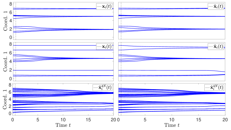
Refer to caption
Figure 3: (Opinion Dynamics) 𝑿(t)𝑿𝑡\boldsymbol{X}(t) (Left column) and 𝑿^(t)^𝑿𝑡\hat{\boldsymbol{X}}(t) (Right column) obtained with the true kernel ϕitalic-ϕ\phi and the estimated interaction kernel ϕ^^italic-ϕ\hat{\phi} from M=16𝑀16M=16 trajectories, for an initial condition in the training data (Top row) and an initial condition randomly chosen (Middle row). The black dashed vertical line at t=0.5𝑡0.5t=0.5 divides the “training” interval [0,0.5]00.5[0,0.5] from the “prediction” interval [0.5, 20]. Bottom row: 𝑿(t)𝑿𝑡\boldsymbol{X}(t) and 𝑿^(t)^𝑿𝑡\hat{\boldsymbol{X}}(t) obtained with ϕitalic-ϕ\phi and ϕ^^italic-ϕ\hat{\phi}, for dynamics with larger Nnew=4Nsubscript𝑁𝑛𝑒𝑤4𝑁N_{new}=4N, over one set of initial conditions. We achieve small error in all cases, in particular predicting the number and location of clusters for large time. The mean of max-in-time trajectory errors over 101010 learning trials can be found in Figure 4.
Refer to caption
Refer to caption
Figure 4: (Opinion Dynamics) Mean errors in trajectory prediction over 10 learning trails using estimated interaction kernels obtained with different values of M𝑀M: for initial conditions in the training set (Training ICs), randomly drawn from μ0subscript𝜇0\mu_{0} (Random ICs), and for a system with 4N4𝑁4N agents (Large N𝑁N). Left: Errors over the training time interval [0,0.5]. Right: Errors over the prediction time interval [0.5,20]. Right upper corner inside the left figure: the learning rate of the relative L2(ρTL)superscript𝐿2superscriptsubscript𝜌𝑇𝐿L^{2}(\rho_{T}^{L}) errors of smoothed estimated interaction kernels. The mean trajectory errors decay at a rate close to the learning rate of interaction kernels, in agreement with Theorem 7.
Refer to caption
Refer to caption
Figure 5: (Opinion Dynamics). Left: The approximate coercivity constant on nsubscript𝑛\mathcal{H}_{n} that consists of piecewise constant functions over n𝑛n uniform partitions of [0,10]010[0,10], obtained from data of 105superscript10510^{5} trajectories. Right: Given true velocities, the learning rate of the estimators is 0.29, close to the theoretical optimal min-max rate 1/313{1}/{3} (shown in the black dot line). Otherwise, for unobserved velocities, the curve of the learning error flattens due to the approximation error of velocities by the finite difference method.

To verify the learnability of the interaction kernel, we estimate the coercivity constant on the hypothesis spaces used in the experiments: we partition [0,10]010[0,10] into n𝑛n uniform subintervals and choose a set of basis functions consisting of the indicator functions, and then use Algorithm 2. We display the estimated coercivity constant of nsubscript𝑛\mathcal{H}_{n} for different values of n𝑛n in Figure 5. These numerical results suggest that the coercivity constant, over L2([0,10],ρTL)superscript𝐿2010superscriptsubscript𝜌𝑇𝐿L^{2}([0,10],\rho_{T}^{L}), is around 0.080.080.08, close to the conjectured lower bound 0.090.090.09 based on Theorem 9. We impute this small difference to the finite sample approximation.
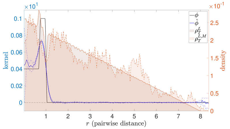
Refer to caption
Figure 6: (Opinion Dynamics) Interaction kernel learned with Unif.([σ,σ])𝜎𝜎([-\sigma,\sigma]) additive noise, for σ=0.15𝜎0.15\sigma=0.15, in the observed positions and observed velocities; here M=128𝑀128M=128, with all the other parameters as in Table 3.

Figure 5 shows that the learning rate of the interaction kernel is M0.3superscript𝑀0.3M^{-0.3}, close to the theoretical optimal rate M1/3superscript𝑀13M^{-{1}/{3}} in Theorem 6 up to a logarithmic factor. An interesting phenomenon is that smoothed learned interaction kernel exhibits a learning rate of M0.45superscript𝑀0.45M^{-0.45} (see upper-right corners of plots in Figure 4). We explain this phenomenon as follows: the gridded interpolation smoothing techniques make our piecewise constant estimators match well with the true kernel, which is almost piecewise constant, and given the lack of noise, it succeeds in reducing the error in the estimator and yielding an almost parametric learning rate.
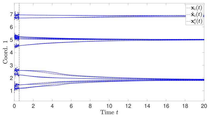
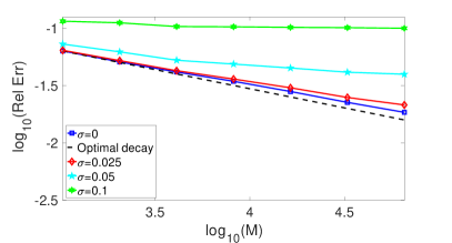
Refer to caption
Figure 7: (Opinion Dynamics) One of the observed trajectories before and after being perturbed by the additive noise. The solid lines represent the true trajectory; the dashed semi-transparent lines represent the noisy trajectory used as training data (together with noisy observations of the velocity); the dash dotted lines are the predicted trajectory learned from the noisy trajectory.
Refer to caption
Refer to caption
Figure 8: (Opinion Dynamics). The learning rates of estimators with different levels of additive noise drawn from Unif.([σ,σ])𝜎𝜎([-\sigma,\sigma]). The noise causes a flattening of the error, with large noise making improvements in the error negligible as the number of observations increases. Left: Rates for estimators without smoothing. Right: Rates for smoothed estimators.

4.3 Predator-Swarm dynamics

There has been a growing literature on modelling interactions between animals of multiple types for the study of animal motion, see Escobedo et al. (2014); Parrish and Edelstein-Keshet (1999); Cohn and Kumar (2009); Nowak (2006); Fryxell et al. (2007). We consider a first-order Predator-Swarm system, modelling interactions between a group of preys and a single predator. The prey-prey interactions have both short-range repulsion to prevent collisions, and long-range attraction to keep the preys in a flock. The preys attract the predator and the predator repels the preys. Since there is only one predator, there are no predator-predator interactions. The intensity of interactions between the single predator and group of preys can be tuned with parameters, determining dynamics with various interesting patterns (from confusing the predator with fast preys, to chasing, to catching up to one prey). We use the set C1subscript𝐶1C_{1} for the set of preys, and the set C2subscript𝐶2C_{2} for the single predator. We consider the interaction kernels

ϕ1,1(r)=1r2,ϕ1,2(r)=2r2,ϕ2,1(r)=3.5r3,ϕ2,2(r)0.formulae-sequencesubscriptitalic-ϕ11𝑟1superscript𝑟2formulae-sequencesubscriptitalic-ϕ12𝑟2superscript𝑟2formulae-sequencesubscriptitalic-ϕ21𝑟3.5superscript𝑟3subscriptitalic-ϕ22𝑟0\phi_{1,1}(r)=1-r^{-2},\quad\phi_{1,2}(r)=-2r^{-2},\quad\phi_{2,1}(r)=3.5r^{-3},\quad\phi_{2,2}(r)\equiv 0.

Since interaction kernels are all singular at r=0𝑟0r=0, we truncate them at rtruncsubscript𝑟truncr_{\text{trunc}} by connecting it with an exponential function of the form aexp(br)𝑎𝑏𝑟a\exp(-br) so that it has continuous derivative on +superscript\mathbb{R}^{+}. The truncation parameters are summarized in Table 4.

kernels rtruncsubscript𝑟truncr_{\text{trunc}}
ϕ1,1subscriptitalic-ϕ11\phi_{1,1} 0.4
ϕ1,2subscriptitalic-ϕ12\phi_{1,2} 111
ϕ2,1subscriptitalic-ϕ21\phi_{2,1} 0.40.40.4
ϕ2,2subscriptitalic-ϕ22\phi_{2,2} 00
Table 4: (PS) Truncation parameters for the Prey-Predator kernels
d𝑑d N1subscript𝑁1N_{1} N2subscript𝑁2N_{2} MρTLsubscript𝑀superscriptsubscript𝜌𝑇𝐿M_{\rho_{T}^{L}} L𝐿L [t1;tL;tf]subscript𝑡1subscript𝑡𝐿subscript𝑡𝑓[t_{1};t_{L};t_{f}] μ0subscript𝜇0\mu_{0} deg(ψkksubscript𝜓𝑘superscript𝑘\psi_{kk^{\prime}}) nkksubscript𝑛𝑘superscript𝑘n_{kk^{\prime}}
222 9 111 105superscript10510^{5}
100
[0;1;20]0120[0;1;20]
Preys: Unif. disk [0,0.5]
Predators: Unif. ring [0.8,1]
1 100(MlogM)15100superscript𝑀𝑀15100(\frac{M}{\log M})^{\frac{1}{5}}
Table 5: (PS) System and learning Parameters for the Predator-Swarming system

In the numerical experiments, the initial positions of the preys are sampled from the uniform distribution on the disk with radius 0.5, and the initial position of the predator is sampled from the uniform distribution in the ring with radii between 0.80.80.8 and 111. The dynamics mimics the following real situation: preys gather and scatter in a small area; the predator approaches the preys gradually and begins to chase the preys within a small distance; although the predator is able to catch up with the swarm as a whole, the individual prey is able to escape by “confusing” the predator: the preys form a ring with the predator at the centre. Finally, they form a flocking behaviour, i.e., they all run in the same direction.

In this example, we assume that the prior information is that each interaction kernel ϕkksubscriptbold-italic-ϕ𝑘superscript𝑘{\bm{\phi}}_{kk^{\prime}} is in the 2-Hölder space, i.e., its derivative is Lipchitz. Note that the true interaction kernels are not compactly supported. However, our theory is still applicable to this case: due to the compact support of μ0subscript𝜇0\mu_{0} and decay of ϕbold-italic-ϕ{\bm{\phi}} at \infty, Grownwall’s inequality implies that, for a sufficiently large R𝑅R (depending only on supp(μ0)suppsubscript𝜇0\text{supp}(\mu_{0}), ϕsubscriptnormbold-italic-ϕ\|{\bm{\phi}}\|_{\infty} and T𝑇T), ϕbold-italic-ϕ{\bm{\phi}} and ϕ1[0,R]bold-italic-ϕsubscript10𝑅{\bm{\phi}}1_{[0,R]} would produce the same dynamics on [0,T]0𝑇[0,T] for any initial conditions sampled from μ0subscript𝜇0\mu_{0}, but now ϕ=ϕ1[0,R]bold-italic-ϕbold-italic-ϕsubscript10𝑅{\bm{\phi}}={\bm{\phi}}1_{[0,R]} is in the function space 𝒦R,Ssubscript𝒦𝑅𝑆\mathcal{K}_{R,S}. Therefore, we can still assume that ϕbold-italic-ϕ{\bm{\phi}} is compactly supported. Here, we choose R=10𝑅10R=10 and nkksubscriptsubscript𝑛𝑘superscript𝑘\mathcal{H}_{n_{kk^{\prime}}} to be the function space that consists of piecewise linear functions on the uniform partition of [0,10] with n𝑛n intervals. It is well-known in approximation theory (e.g. DeVore and Lucier (1992)) that infφnφϕkk1[0,10]Lip[ϕkk]n2subscriptinfimum𝜑subscript𝑛subscriptnorm𝜑subscriptitalic-ϕ𝑘superscript𝑘subscript1010Lipdelimited-[]superscriptsubscriptitalic-ϕ𝑘superscript𝑘superscript𝑛2\inf_{\varphi\in\mathcal{H}_{n}}\|\varphi-\phi_{kk^{\prime}}1_{[0,10]}\|_{\infty}\leq\text{Lip}[\phi_{kk^{\prime}}^{{}^{\prime}}]n^{-2}. Therefore the conditions in Theorem 6 are satisfied with s=2𝑠2s=2. Our theory suggests that any choice of dimension n𝑛n that is proportional to (MlogM)1/5superscript𝑀𝑀15(\frac{M}{\log M})^{{1}/{5}} yields an optimal learning rate M25superscript𝑀25M^{-\frac{2}{5}}, up to a logarithmic factor. We choose n=100(MlogM)1/5𝑛100superscript𝑀𝑀15n=100(\frac{M}{\log M})^{{1}/{5}} here. The system and learning parameters for Predator-Swarm dynamics are summarized in Table 5.
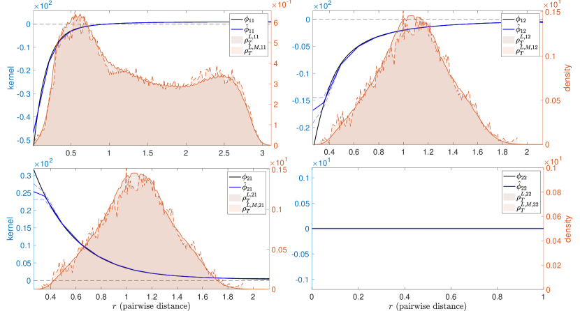
Refer to caption
Refer to caption
Figure 9: (Predator-Swarm Dynamics) Comparison between true and estimated interaction kernels with M=16𝑀16M=16 (Top) and 102410241024 (Bottom). In black: the true interaction kernels. In blue: the learned interaction kernels using piecewise linear functions. When M𝑀M increases from 16 to 102410241024, the standard deviation bars on the estimated interaction kernels become smaller and less visible. The relative errors in 𝑳2(𝝆TL)superscript𝑳2superscriptsubscript𝝆𝑇𝐿\boldsymbol{L}^{2}(\bm{\rho}_{T}^{L}) for the interaction kernels are (9±2)103plus-or-minus92superscript103(9\pm 2)\cdot 10^{-3} and (2.5±0.05)103plus-or-minus2.50.05superscript103(2.5\pm 0.05)\cdot 10^{-3}.

Figure 9 indicates that the estimators match the true interaction kernels extremely well except for a small bias at locations near 0. We impute this error near 0 to two reasons: (i) the strong short-range repulsion between agents force the pairwise distances to stay bounded away from r=0𝑟0r=0, yielding a 𝝆TLsuperscriptsubscript𝝆𝑇𝐿\bm{\rho}_{T}^{L} that is nearly singular near 0, so that there are only a few samples to learn the interaction kernels near 00. We see that as M𝑀M increases, the error near 0 is getting smaller, and we expect it to converge to 00. (ii) Information of ϕ(0)bold-italic-ϕ0{\bm{\phi}}(0) is lost due to the structure of the equations, as we mentioned earlier in the previous example, which may cause the error in the finite difference approximation of velocities to affect the reconstruction of values near 00.

Refer to caption
Figure 10: (PS) 𝑿(t)𝑿𝑡\boldsymbol{X}(t) and 𝑿^(t)^𝑿𝑡\hat{\boldsymbol{X}}(t) obtained with ϕbold-italic-ϕ{\bm{\phi}} and ϕ^^bold-italic-ϕ\hat{\bm{\phi}} learned from M=16𝑀16M=16 trajectories respectively: for an initial condition in the training data (Top) and an initial condition randomly chosen (Middle). The black dot at t=1𝑡1t=1 divides the “training” interval [0,1]01[0,1] from the “prediction” interval [1, 20]. Bottom: 𝑿(t)𝑿𝑡\boldsymbol{X}(t) and 𝑿^(t)^𝑿𝑡\hat{\boldsymbol{X}}(t) obtained with ϕitalic-ϕ\phi and ϕ^^italic-ϕ\hat{\phi} learned from M=16𝑀16M=16 trajectories respectively, for dynamics with larger Nnew=4Nsubscript𝑁𝑛𝑒𝑤4𝑁N_{new}=4N, over a set of initial conditions. We achieve small errors in all cases, in particular we predict successfully the flocking time and direction. The means of trajectory errors can be found in Figure 11.

Figure 10 shows that with a rather small M𝑀M, the learned interaction kernels not only produce an accurate approximation of the transient behaviour of the agents over the training time interval [t1,tL]subscript𝑡1subscript𝑡𝐿[t_{1},t_{L}], but also of the flocking behaviour over the large time interval [tL,tf]subscript𝑡𝐿subscript𝑡𝑓[t_{L},t_{f}] including the time of formation and the direction of a flocking, which is perhaps beyond expectations.

Figure 11 shows that the mean trajectory errors over 10 learning trials decay with M𝑀M at a rate 0.32 on the training time interval [0,1]01[0,1], matching the learning rate of smoothed kernels, even in the case of a new system with 4N4𝑁4N agents. This agrees with Theorem 7 on the learning rate of trajectories over the training time. For the prediction time interval [1,20]120[1,20], our learned interaction kernels also produced very accurate approximations of true trajectories in all cases, see Figure 11.

Next, we study the learnability of the estimated interaction kernels in this system. As demonstrated by Proposition 8, the coercivity constant is the minimal eigenvalue of AL,,𝓗subscript𝐴𝐿𝓗A_{L,\infty,\boldsymbol{\mathcal{H}}}, which in our cases is blocked diagonal: one block for learning prey-prey and prey-predator interactions from velocities of preys, and the other block for learning predator-prey interaction from velocities of the predator. We display the minimal eigenvalues for each block in Figure 12. We see that the minimal eigenvalue of the prey-prey block matrix stays around 21022superscript1022\cdot 10^{-2} and the predator-predator matrix stays around 0.71020.7superscript1020.7\cdot 10^{-2} as partitions get finer. We therefore conjecture that the coercivity constant over 𝑳2([0,10],𝝆TL)superscript𝑳2010superscriptsubscript𝝆𝑇𝐿\boldsymbol{L}^{2}([0,10],\bm{\rho}_{T}^{L}) is about 0.71020.7superscript1020.7\cdot 10^{-2}.

When true velocities are observed, we obtain a learning rate for ϕ^()ϕ()L2(𝝆TL)\|\hat{\bm{\phi}}(\cdot)\cdot-{\bm{\phi}}(\cdot)\cdot\|_{L^{2}(\bm{\rho}_{T}^{L})} around M0.35superscript𝑀0.35M^{-0.35} (logM/M)0.4\log M/M)^{-0.4}) (see Figure 12), which matches our theoretical results and is close to the optimal min-max rate M2/5superscript𝑀25M^{-{2}/{5}} for regression with noisy observations up to a logarithmic factor. If the velocities were not observed, the learning rate would be affected. In the right upper corner of Figure 11, we see that the learning rate of the smoothed estimators is around M0.32superscript𝑀0.32M^{-0.32} if we use the finite difference method to estimate the unobserved velocities, leading to an error in the velocities of size O(102)𝑂superscript102O(10^{-2}).

Refer to caption
Refer to caption
Figure 11: (Predator-Swarm Dynamics) Mean errors in trajectory prediction over 10 learning trials using estimated interaction kernels obtained with different values of M𝑀M: for initial conditions in the training set (Training ICs), randomly drawn from μ0subscript𝜇0\mu_{0} (Random ICs), and for a system with 4N4𝑁4N agents (Large N𝑁N). Left: Errors over the training time interval [0,1]. Right: Errors over the future time interval [1,20]. Upper right corner of left figure: the learning rate of the smoothed learned interaction kernels. The decay rate of the mean trajectory prediction errors over the training time is faster than that of interaction kernels. On the prediction time interval, we still achieve good accuracy for trajectories, with a rate a bit slower than that of interaction kernels.
Refer to caption
Refer to caption
Figure 12: (PS). Left: The coercivity constant on nsubscript𝑛\mathcal{H}_{n} consisting of piecewise linear functions over n𝑛n-uniform partitions of the support of 𝝆TLsuperscriptsubscript𝝆𝑇𝐿\bm{\rho}_{T}^{L}, computed from data consisting of M=105𝑀superscript105M=10^{5} trajectories.Right: the relative L2(𝝆TL)superscript𝐿2superscriptsubscript𝝆𝑇𝐿L^{2}(\bm{\rho}_{T}^{L}) errors decay at a rate about (M)0.35superscript𝑀0.35(M)^{-0.35}, close to theoretical optimal min-max rate.
Refer to caption
Figure 13: (Predator-Swarm Dynamics) Interaction kernels learned with Unif.([σ,σ])𝜎𝜎([-\sigma,\sigma]) multiplicative noise, for σ=0.1𝜎0.1\sigma=0.1, in the observed positions and observed velocities; here M=16𝑀16M=16, with all the other parameters as in Table 5.
Refer to caption
Figure 14: (Predator-Swarm Dynamics) One of the observed trajectories before and after being perturbed by the multiplicative noise drawn from Unif.([σ,σ])𝜎𝜎([-\sigma,\sigma]) with σ=0.1𝜎0.1\sigma=0.1. The solid lines represent the true trajectory; the dashed semi-transparent lines represent the noisy trajectory used as training data (together with noisy observations of the velocity); the dash dotted lines are the predicted trajectory learned from the noisy trajectory.
Refer to caption
Refer to caption
Figure 15: (Predator-Swarm Dynamics). The learning rates of estimators with different levels of multiplicative noise drawn from Unif.([σ,σ])𝜎𝜎([-\sigma,\sigma]). The noise make the learning curve tend to be flat as its level increases. Left: Rates for estimators without smoothing. Right: Rates for smoothed estimators.

4.4 Heterogeneous particle dynamics

We consider here another representative heterogeneous agent dynamics: a particle system with two types of particles (denoted by α𝛼\alpha and β𝛽\beta) governed by Lennard-Jones type potentials (a popular choice for example to model atom-atom interactions in molecular dynamics and materials sciences). The general expression of the Lennard-Jones type potential is

Φ(r)=pϵ(pq)[qp(rmr)p(rmr)q]Φ𝑟𝑝italic-ϵ𝑝𝑞delimited-[]𝑞𝑝superscriptsubscript𝑟𝑚𝑟𝑝superscriptsubscript𝑟𝑚𝑟𝑞\Phi(r)=\frac{p\epsilon}{(p-q)}\left[\frac{q}{p}\left(\frac{r_{m}}{r}\right)^{p}-\left(\frac{r_{m}}{r}\right)^{q}\right]

where ϵitalic-ϵ\epsilon is the depth of the potential well, r𝑟r is the distance between the particles, and rmsubscript𝑟𝑚r_{m} is the distance at which the potential reaches its minimum. At rmsubscript𝑟𝑚r_{m}, the potential function has the value ϵitalic-ϵ-\epsilon. The rpsuperscript𝑟𝑝r^{-p} term, which is the repulsive term, describes Pauli repulsion at short ranges due to overlapping electron orbitals, and the rqsuperscript𝑟𝑞r^{-q} term, which is the attractive long-range term, describes attraction at long ranges (modeling van der Waals forces, or dispersion forces). Note that the corresponding Lennard-Jones type kernel ϕ(r)=Φ(r)ritalic-ϕ𝑟superscriptΦ𝑟𝑟\phi(r)=\frac{\Phi^{\prime}(r)}{r} is singular at r=0𝑟0r=0: we truncate it at rtruncsubscript𝑟truncr_{\text{trunc}} by connecting it with an exponential function of the form aexp(br12)𝑎𝑏superscript𝑟12a\exp(-br^{12}) so that it is continuous with a continuous derivative on +superscript\mathbb{R}^{+}.

Refer to caption
Refer to caption
Figure 16: (Lennard Jones Dynamics) Comparison between true and estimated interaction kernels with M=16𝑀16M=16 (Top) and M=512𝑀512M=512 (Bottom). In black: the true interaction kernels. In blue: the learned interaction kernels using piecewise linear functions. The learned interaction kernels with M=16𝑀16M=16 match the true kernels very well except at the region near 0. For a larger M=512𝑀512M=512, the learned interaction kernels match more faithfully to the true interaction kernels at locations near 0; the standard deviation bars on the estimated interaction kernels become smaller and less visible. The relative errors in 𝑳2(𝝆TL)superscript𝑳2superscriptsubscript𝝆𝑇𝐿\boldsymbol{L}^{2}(\bm{\rho}_{T}^{L}) norm for the kernels are (4±2)102plus-or-minus42superscript102(4\pm 2)\cdot 10^{-2} and (1.2±0.003.5)102plus-or-minus1.20.003.5superscript102(1.2\pm 0.003.5)\cdot 10^{-2}.

In our notation for heterogeneous systems, the set C1subscript𝐶1C_{1} corresponds to α𝛼\alpha-particles, and C2subscript𝐶2C_{2} corresponds to β𝛽\beta-particles. The intensity of interaction(s) between particles can be tuned with parameters, determining different types of mixture of particles. In the numerical simulations, we consider interaction kernels ϕ1,1subscriptitalic-ϕ11\phi_{1,1}, ϕ1,2subscriptitalic-ϕ12\phi_{1,2}, ϕ2,1subscriptitalic-ϕ21\phi_{2,1} and ϕ2,2subscriptitalic-ϕ22\phi_{2,2} with parameters summarized in Table 6.

kernels p𝑝p q𝑞q ϵitalic-ϵ\epsilon rmsubscript𝑟𝑚r_{m} rtruncsubscript𝑟truncr_{\text{trunc}}
ϕ1,1subscriptitalic-ϕ11\phi_{1,1} 444 1 101010 0.80.80.8 0.68
ϕ1,2subscriptitalic-ϕ12\phi_{1,2} 888 2 1.51.51.5 0.50.50.5 0.40.40.4
ϕ2,1subscriptitalic-ϕ21\phi_{2,1} 888 2 1.51.51.5 0.50.50.5 0.40.40.4
ϕ2,2subscriptitalic-ϕ22\phi_{2,2} 555 2 555 111 0.80.80.8
Table 6: (LJ) Parameters for the Lennard Jones kernels
d𝑑d N1subscript𝑁1N_{1} N2subscript𝑁2N_{2} MρTLsubscript𝑀superscriptsubscript𝜌𝑇𝐿M_{\rho_{T}^{L}} L𝐿L [t1;tL;tf]subscript𝑡1subscript𝑡𝐿subscript𝑡𝑓[t_{1};t_{L};t_{f}] μ0subscript𝜇0\mu_{0} deg(ψkksubscript𝜓𝑘superscript𝑘\psi_{kk^{\prime}}) nkksubscript𝑛𝑘superscript𝑘n_{kk^{\prime}}
222 5 555 105superscript10510^{5}
100
[0;0.05;2]00.052[0;0.05;2] 𝒩(0,I20×20)𝒩0subscript𝐼2020\mathcal{N}(\textbf{0},I_{20\times 20}) 1 300(MlogM)15300superscript𝑀𝑀15300(\frac{M}{\log M})^{\frac{1}{5}}
Table 7: (LJ) Parameters for the system

In the experiments, the particles are drawn i.i.d from standard Gaussian distribution in 2. In this system, the particle-particle interactions are all short-range repulsions and long-range attractions. The short-range repulsion force prevents the particles to collide and long-range attractions keep the particles in the flock. Both the α𝛼\alpha-particles and β𝛽\beta-particles form the crystal-like clusters. Moreover, the α𝛼\alpha-β𝛽\beta potential function is the same with the β𝛽\beta-α𝛼\alpha potential function. Both of them have the smallest rmsubscript𝑟𝑚r_{m} and relative large attractive force (see Table 6) when an α𝛼\alpha-particle is far from a β𝛽\beta-particle. As a result, the attraction force between two different types of particles will force them to mix homogeneously.

Since the system evolves to equilibrium configurations very quickly, we observe the dynamics up to a time tLsubscript𝑡𝐿t_{L} which is a fraction of the equilibrium time. Since the particles only explore a bounded region due to the large-range attraction, 𝝆TLsuperscriptsubscript𝝆𝑇𝐿\smash{\bm{\rho}_{T}^{L}} is essentially supported on a bounded region (see the histogram background of Figure 16), on which the interaction kernels are in the 2-Hölder space. Therefore, our learning theory is still applicable in this case. Similar to the learning in Predator-Swarm dynamics, the estimator of each ϕkksubscriptitalic-ϕ𝑘superscript𝑘\phi_{kk^{\prime}} belongs to a piecewise linear function space over a uniform partition of n𝑛n intervals. The observation and learning parameters are summarized in Table 7. As reported in Figure 16, with rather small M𝑀M, the learned interaction kernels ϕ^^bold-italic-ϕ\widehat{\bm{\phi}} approximate the true interaction kernels ϕbold-italic-ϕ{\bm{\phi}} very well in the regions with large 𝝆TLsuperscriptsubscript𝝆𝑇𝐿\bm{\rho}_{T}^{L}, i.e., regions with an abundance of observed values of pairwise distances to reconstruct the interaction kernels. The reasons for the error near 0 are similar to those for Predator-Swarm dynamics.
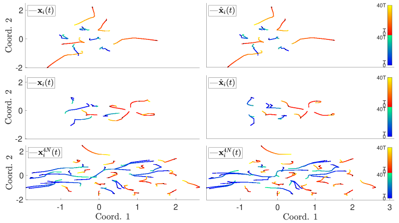
Refer to caption
Figure 17: (Lennard Jones Dynamics) 𝑿(t)𝑿𝑡\boldsymbol{X}(t) and 𝑿^(t)^𝑿𝑡\hat{\boldsymbol{X}}(t) obtained with ϕbold-italic-ϕ{\bm{\phi}} and ϕ^^bold-italic-ϕ\widehat{\bm{\phi}} learned with M=16𝑀16M=16 for an initial condition in the training data (Top row) and a new initial condition random drawn from μ0subscript𝜇0\mu_{0} (Middle row). The black dot at t=0.05𝑡0.05t=0.05 divides the training time interval [0,0.05]00.05[0,0.05] from the prediction time interval [0.05, 2]. Bottom row: 𝑿(t)𝑿𝑡\boldsymbol{X}(t) and 𝑿^(t)^𝑿𝑡\hat{\boldsymbol{X}}(t) obtained with ϕitalic-ϕ\phi and ϕ^^italic-ϕ\hat{\phi} learned from M=16𝑀16M=16 trajectories respectively, for dynamics with larger Nnew=4Nsubscript𝑁𝑛𝑒𝑤4𝑁N_{new}=4N, over a set of initial conditions. We achieve small errors, in average, in particular predicting the time and shape of particle aggregation. The means of trajectory prediction errors are in Figure 18.

Figure 17 shows that the learned interaction kernels not only produce an accurate approximation of transient behaviour of particles on the training time interval [t1,tL]subscript𝑡1subscript𝑡𝐿[t_{1},t_{L}], but also the aggregation of particles over a much larger prediction time interval [tL,tf]subscript𝑡𝐿subscript𝑡𝑓[t_{L},t_{f}].

Refer to caption
Refer to caption
Figure 18: (Lennard Jones Dynamics) Mean errors in trajectory prediction over 10 learning trails using estimated interaction kernels obtained with different values of M𝑀M: for initial conditions in the training set (Training ICs), randomly drawn from μ0subscript𝜇0\mu_{0} (Random ICs), and for a system with 4N4𝑁4N agents (Large N𝑁N). Left: Errors over the training time interval [0, 0.05]. Right: Errors over the future time interval [0.05, 2]. Upper right corner of left figure: the learning rate of kernels (used to predict dynamics). The learning curves of trajectory prediction errors over the training time interval are almost the same with those of interaction kernels. On the prediction time interval, we still achieve a good accuracy of trajectory prediction and just a slightly slower rate for predicting trajectories in all cases.

We summarize the mean trajectory prediction errors over 10 learning trials in Figure 18. It shows that the learning rate of the trajectory errors over the training time interval [0,0.05]00.05[0,0.05] is the same with the learning rate of the kernels. For the prediction time interval [0.05,2]0.052[0.05,2], our learned interaction kernels still produced very accurate approximations of true trajectories in all cases, as demonstrated in Figure 18.

We then compute the minimal eigenvalue of AL,,𝓗subscript𝐴𝐿𝓗A_{L,\infty,\boldsymbol{\mathcal{H}}}, inspired by Proposition 8. In this case, AL,,𝓗subscript𝐴𝐿𝓗A_{L,\infty,\boldsymbol{\mathcal{H}}} is block diagonal: one block for learning ϕ1,1subscriptitalic-ϕ11\phi_{1,1} and ϕ1,2subscriptitalic-ϕ12\phi_{1,2} from velocities of α𝛼\alpha-particles, and the other block for learning ϕ2,1subscriptitalic-ϕ21\phi_{2,1} and ϕ2,2subscriptitalic-ϕ22\phi_{2,2} from velocities of the β𝛽\beta-particles. We display the minimal eigenvalues for each block in Figure 19. We see that the minimal eigenvalue of the type 1 block matrix stay around 8.71028.7superscript1028.7\cdot 10^{-2} and the type 2 block matrix stay around 8.91028.9superscript1028.9\cdot 10^{-2} as the partitions get finer, suggesting a positive coercivity constant over 𝑳2(𝝆TL)superscript𝑳2superscriptsubscript𝝆𝑇𝐿\boldsymbol{L}^{2}(\bm{\rho}_{T}^{L}).

Refer to caption
Refer to caption
Figure 19: Left: The coercivity constant on nsubscript𝑛\mathcal{H}_{n} consisting of piecewise linear functions over n𝑛n-uniform partitions of the support of 𝝆TLsuperscriptsubscript𝝆𝑇𝐿\bm{\rho}_{T}^{L}, computed from data consisting of M=105𝑀superscript105M=10^{5} trajectories. Right: the relative L2(𝝆TL)superscript𝐿2superscriptsubscript𝝆𝑇𝐿L^{2}(\bm{\rho}_{T}^{L}) errors decay at a rate M0.35superscript𝑀0.35M^{-0.35}, close to theoretical optimal min-max rate M0.4superscript𝑀0.4M^{-0.4} up to a logarithmic factor (shown in the black dot line) as in Theorem 6.

We choose the partition number nkksubscript𝑛𝑘superscript𝑘n_{kk^{\prime}} for learning ϕkksubscriptitalic-ϕ𝑘superscript𝑘\phi_{kk^{\prime}} according to Theorem 6. Given true velocities, we obtain a learning rate for ϕ^()ϕ()L2(𝝆TL)\smash{\|\hat{\bm{\phi}}(\cdot)\cdot-{\bm{\phi}}(\cdot)\cdot\|_{L^{2}(\bm{\rho}_{T}^{L})}} around M0.35superscript𝑀0.35M^{-0.35} (see right column of Figure 19), which is close to the theoretical optimal min-max rate M2/5superscript𝑀25M^{-{2}/{5}}. The error in finite difference approximation of the velocities affects the learning rate, as is demonstrated in the right upper corner of Figure 18, where the learning curves tends to flatten.
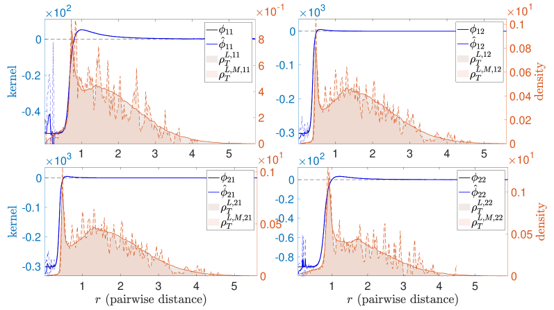
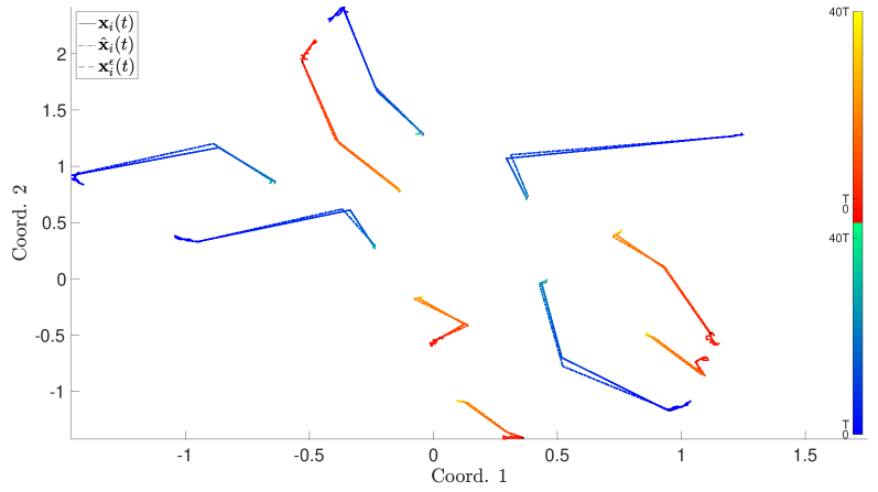
Refer to caption
Figure 20: (Lennard Jones Dynamics) Interaction kernels learned with Unif.([σ,σ])𝜎𝜎([-\sigma,\sigma]) additive noise, for σ=0.02𝜎0.02\sigma=0.02, in the observed positions and observed velocities; here M=16𝑀16M=16, with all the other parameters as in Table 7.
Refer to caption
Figure 21: (Lennard Jones Dynamics) One of the observed trajectories before and after being perturbed by the additive noise drawn from Unif.([σ,σ])𝜎𝜎([-\sigma,\sigma]) with σ=0.02𝜎0.02\sigma=0.02. The solid lines represent the true trajectory; the dashed semi-transparent lines represent the noisy trajectory used as training data (together with noisy observations of the velocity); the dash dotted lines are the predicted trajectory learned from the noisy trajectory.
Refer to caption
Refer to caption
Figure 22: (Lennard Jones Dynamics). The learning rates of estimators with different levels of additive noise drawn from Unif.([σ,σ])𝜎𝜎([-\sigma,\sigma]). Left: Rates for estimators without smoothing. Right: Rates for smoothed estimators.

4.5 Summary of the numerical experiments

  • Short time observations don’t prevent us from learning the interaction kernels. The randomness of initial conditions enables the agents to explore large regions of state space, and in the space of pairwise distance in a short time. The estimated interaction kernels approximate well in the regions where 𝝆TLsuperscriptsubscript𝝆𝑇𝐿\bm{\rho}_{T}^{L} is large, i.e. regions with an abundance pairwise distances to reconstruct the interaction kernels. As the number of trajectories increases, we obtain more faithful approximations of the true interaction kernels, agreeing with the consistency Theorem 5. We also see that our estimators, even learned from a small amount of data sampled from a short period of transient dynamics, not only can predict the dynamics on the training time interval [t1,tL]subscript𝑡1subscript𝑡𝐿[t_{1},t_{L}] but also produce accurate predictions of large time behaviour of the system.

  • The decay rate of the mean trajectory prediction errors over the training time interval [t1,tL]subscript𝑡1subscript𝑡𝐿[t_{1},t_{L}] in terms of M𝑀M is the same with the learning rate of the estimated interaction kernels (that are used to predict dynamics), agreeing with Theorem 7.

  • The coercivity condition holds on hypothesis spaces that consist of piecewise polynomials, for different kernel functions, and various initial distributions including Gaussian and uniform distributions, and for different L𝐿L. The learning rates of the kernels match closely the rate we derived in Theorem 6, which are optimal up to a logarithmic factor.

  • Our estimators are robust to the observational noise up to a certain level and still produced rather accurate predictions of the true dynamics. The learning rate of interaction kernels tends to be flat as the noise level increases, showing our estimators do not overcome the problem exhibited by other estimators of ODEs and PDEs, and do not denoise and recover the true interaction kernel even asymptotically. When the noise is significant, the accuracy of the estimators did not improve as the number of observed trajectories increased.

5 Discussions on the coercivity condition

The coercivity condition on the hypothesis space 𝓗𝓗\boldsymbol{\mathcal{H}}, quantized by the constant cL,N,𝓗subscript𝑐𝐿𝑁𝓗c_{L,N,\boldsymbol{\mathcal{H}}}, plays a vital role in establishing the optimal convergence rate, as is demonstrated in Theorem 4 and Theorem 6. Proposition 8 provides a way to compute the coercivity constant on a finite dimensional 𝓗𝓗\boldsymbol{\mathcal{H}} numerically: it is the minimal eigenvalue of the matrix that yields the estimator by choosing an orthonormal basis of 𝑳2([0,R],𝝆TL)superscript𝑳20𝑅superscriptsubscript𝝆𝑇𝐿\boldsymbol{L}^{2}([0,R],\bm{\rho}_{T}^{L}). We have performed extensive numerical experiments to test the coercivity condition for different dynamical systems. Numerical results suggest that the coercivity condition holds true on rather general hypothesis space for a large class of kernel functions, and for various initial distributions including Gaussian and uniform distributions, and for different values of L𝐿L as long as 𝝆TLsuperscriptsubscript𝝆𝑇𝐿\bm{\rho}_{T}^{L} is not degenerate.

In the following, we prove the coercivity condition on general compact sets of 𝑳2([0,R],𝝆TL)superscript𝑳20𝑅superscriptsubscript𝝆𝑇𝐿\boldsymbol{L}^{2}([0,R],\bm{\rho}_{T}^{L}) under suitable hypotheses, and even independently of N𝑁N. This implies that the finite sample bounds we achieved in Theorem 6 can be dimension free, suggesting that the coercivity condition may be a fundamental property of the system, even in the mean field limit.

5.1 Homogeneous systems

In a homogeneous system, it is natural to assume the distribution μ0subscript𝜇0\mu_{0} of initial conditions is exchangeable (i.e., the distribution is invariant under permutation of components). We prove the coercivity condition for exchangeable Gaussian distributions in the case of L=1𝐿1L=1. We show that cL,N,subscript𝑐𝐿𝑁c_{L,N,\mathcal{H}} can be bounded below by a positive constant that is independent of N𝑁N for any compact set \mathcal{H} in L2([0,R],ρTL)superscript𝐿20𝑅superscriptsubscript𝜌𝑇𝐿L^{2}([0,R],\rho_{T}^{L}). A key element is connect the coercivity with the strict positiveness of an integral operator, which follows from a Müntz-Szász-type Theorem. We refer to Li et al. (2019) for a further study on the coercivity condition for stochastic homogeneous systems.

Theorem 9

Consider the system at time t1=0subscript𝑡10t_{1}=0 with initial distribution 𝛍0subscript𝛍0{\bm{\mu}}_{0} being exchangeable Gaussian with cov(𝐱i(t1))cov(𝐱i(t1),𝐱j(t1))=λIdcovsubscript𝐱𝑖subscript𝑡1covsubscript𝐱𝑖subscript𝑡1subscript𝐱𝑗subscript𝑡1𝜆subscript𝐼𝑑\mathrm{cov}(\boldsymbol{x}_{i}(t_{1}))-\mathrm{cov}(\boldsymbol{x}_{i}(t_{1}),\boldsymbol{x}_{j}(t_{1}))=\lambda I_{d}  for a constant λ>0𝜆0\lambda>0. Then the coercivity condition holds true on =L2([0,R],ρT1)superscript𝐿20𝑅subscriptsuperscript𝜌1𝑇\mathcal{H}=L^{2}([0,R],\rho^{1}_{T}) with the coercivity constant cL,N,=N1N2subscript𝑐𝐿𝑁𝑁1superscript𝑁2c_{L,N,\mathcal{H}}=\frac{N-1}{N^{2}}. If the hypothesis space \mathcal{H} is a compact subset of L2([0,R],ρT1)superscript𝐿20𝑅subscriptsuperscript𝜌1𝑇L^{2}([0,R],\rho^{1}_{T}), then we have cL,N,=N1N2+(N1)(N2)N2csubscript𝑐𝐿𝑁𝑁1superscript𝑁2𝑁1𝑁2superscript𝑁2subscript𝑐c_{L,N,\mathcal{H}}=\frac{N-1}{N^{2}}+\frac{(N-1)(N-2)}{N^{2}}c_{\mathcal{H}} for its coercivity constant, where c>0subscript𝑐0c_{\mathcal{H}}>0 is independent of N𝑁N.

Proof  With L=1𝐿1L=1, the right hand side of the coercivity inequality (2.9) is

𝔼μ0[𝐟φ(𝑿(t1))𝒮2]subscript𝔼subscript𝜇0delimited-[]superscriptsubscriptnormsubscript𝐟𝜑𝑿subscript𝑡1𝒮2\displaystyle\mathbb{E}_{\mu_{0}}[\big{\|}\mathbf{f}_{\varphi}(\boldsymbol{X}(t_{1}))\big{\|}_{\mathcal{S}}^{2}] =1N3i=1N𝔼μ0[(j=k=1N+jk=1N)φ(𝒙ji(t1))φ(𝒙ki(t1))𝒙ji(t1),𝒙ki(t1)]absent1superscript𝑁3superscriptsubscript𝑖1𝑁subscript𝔼subscript𝜇0delimited-[]superscriptsubscript𝑗𝑘1𝑁superscriptsubscript𝑗𝑘1𝑁𝜑normsubscript𝒙𝑗𝑖subscript𝑡1𝜑normsubscript𝒙𝑘𝑖subscript𝑡1subscript𝒙𝑗𝑖subscript𝑡1subscript𝒙𝑘𝑖subscript𝑡1\displaystyle=\frac{1}{N^{3}}\sum_{i=1}^{N}\mathbb{E}_{\mu_{0}}\bigg{[}\left(\sum_{j=k=1}^{N}+\sum_{j\neq k=1}^{N}\right)\varphi(\|\boldsymbol{x}_{ji}(t_{1})\|)\varphi(\|\boldsymbol{x}_{ki}(t_{1})\|)\langle\boldsymbol{x}_{ji}(t_{1}),\boldsymbol{x}_{ki}(t_{1})\big{\rangle}\bigg{]}
=N1N2φ()L2([0,R],ρT1)2+,\displaystyle=\frac{N-1}{N^{2}}\|\varphi(\cdot)\cdot\|_{L^{2}([0,R],\rho_{T}^{1})}^{2}+\mathcal{R}, (5.1)

where =1N3i=1Njk,ji,kiCijk1superscript𝑁3superscriptsubscript𝑖1𝑁subscriptformulae-sequence𝑗𝑘formulae-sequence𝑗𝑖𝑘𝑖subscript𝐶𝑖𝑗𝑘\mathcal{R}=\frac{1}{N^{3}}\sum_{i=1}^{N}\sum_{j\neq k,j\neq i,k\neq i}C_{ijk} with

Cijk:=𝔼[φ(𝒙ji(t1))φ(𝒙ki(t1))𝒙ji(t1),𝒙ki(t1)],assignsubscript𝐶𝑖𝑗𝑘𝔼delimited-[]𝜑normsubscript𝒙𝑗𝑖subscript𝑡1𝜑normsubscript𝒙𝑘𝑖subscript𝑡1subscript𝒙𝑗𝑖subscript𝑡1subscript𝒙𝑘𝑖subscript𝑡1\displaystyle C_{ijk}:=\mathbb{E}\bigg{[}\varphi(\|\boldsymbol{x}_{ji}(t_{1})\|)\varphi(\|\boldsymbol{x}_{ki}(t_{1})\|)\langle\boldsymbol{x}_{ji}(t_{1}),\boldsymbol{x}_{ki}(t_{1})\big{\rangle}\bigg{]},

Because of exchangeability, we have

Cijk=𝔼[φ(YX)φ(ZX)YX,ZX]subscript𝐶𝑖𝑗𝑘𝔼delimited-[]𝜑norm𝑌𝑋𝜑norm𝑍𝑋𝑌𝑋𝑍𝑋\displaystyle C_{ijk}=\mathbb{E}\bigg{[}\varphi(\|Y-X\|)\varphi(\|Z-X\|)\left\langle Y-X,Z-X\right\rangle\bigg{]}

for all (i,j,k)𝑖𝑗𝑘(i,j,k), where X,Y,Z𝑋𝑌𝑍X,Y,Z are exchangeable Gaussian random variables with cov(X)cov(X,Y)=λIdcov𝑋cov𝑋𝑌𝜆subscript𝐼𝑑\mathrm{cov}(X)-\mathrm{cov}(X,Y)=\lambda I_{d}. By Lemma 10 below, Cijkcφ()L2([0,R],ρT1)2C_{ijk}\geq c_{\mathcal{H}}\|\varphi(\cdot)\cdot\|_{L^{2}([0,R],\rho_{T}^{1})}^{2}. Therefore, (N1)(N2)N2cφ()L2([0,R],ρT1)2\mathcal{R}\geq\frac{(N-1)(N-2)}{N^{2}}c_{\mathcal{H}}\|\varphi(\cdot)\cdot\|_{L^{2}([0,R],\rho_{T}^{1})}^{2}, and φ,φ(N1N2+(N1)(N2)N2c)φ()L2([0,R],ρT1)2.\langle\langle{\varphi,\varphi}\rangle\rangle\geq(\frac{N-1}{N^{2}}+\frac{(N-1)(N-2)}{N^{2}}c_{\mathcal{H}})\|\varphi(\cdot)\cdot\|^{2}_{L^{2}([0,R],\rho_{T}^{1})}\,.  

The following lemma is a key element in the above proof of the coercivity condition.

Lemma 10

Let X,Y,Z𝑋𝑌𝑍X,Y,Z be exchangeable Gaussian random vectors in d with cov(X)cov(X,Y)=λIdcov𝑋cov𝑋𝑌𝜆subscript𝐼𝑑\mathrm{cov}(X)-\mathrm{cov}(X,Y)=\lambda I_{d} for a constant λ>0𝜆0\lambda>0. Let ρT1superscriptsubscript𝜌𝑇1\rho_{T}^{1} be a probability measure over + with density function Cλ1rd1e14λr2superscriptsubscript𝐶𝜆1superscript𝑟𝑑1superscript𝑒14𝜆superscript𝑟2C_{\lambda}^{-1}r^{d-1}e^{-\frac{1}{4\lambda}r^{2}} where Cλ=12(4λ)d2Γ(d2)subscript𝐶𝜆12superscript4𝜆𝑑2Γ𝑑2C_{\lambda}=\frac{1}{2}(4\lambda)^{\frac{d}{2}}\Gamma(\frac{d}{2}). Then,

𝔼[φ(|XY|)φ(|XZ|)XY,XZ]c𝒳φ()L2(ρT1)2\mathbb{E}\left[\varphi(|X-Y|)\varphi(|X-Z|)\langle X-Y,X-Z\rangle\right]\geq c_{\mathcal{\mathcal{X}}}\|\varphi(\cdot)\cdot\|^{2}_{L^{2}(\rho_{T}^{1})} (5.2)

for all φ()𝒳\varphi(\cdot)\cdot\in\mathcal{X}, with c𝒳>0subscript𝑐𝒳0c_{\mathcal{X}}>0 if 𝒳𝒳\mathcal{X} is compact and c𝒳=0subscript𝑐𝒳0c_{\mathcal{X}}=0 if 𝒳=L2([0,R],ρT1)𝒳superscript𝐿20𝑅superscriptsubscript𝜌𝑇1\mathcal{X}=L^{2}([0,R],\rho_{T}^{1}).

Proof  Let (U,V)=(XY,XZ)𝑈𝑉𝑋𝑌𝑋𝑍(U,V)=(X-Y,X-Z). Note that the covariance matrix of (U,V)𝑈𝑉(U,V) is λ(2IdIdId2Id)𝜆matrix2subscript𝐼𝑑subscript𝐼𝑑subscript𝐼𝑑2subscript𝐼𝑑\lambda\begin{pmatrix}2I_{d}&I_{d}\\ I_{d}&2I_{d}\end{pmatrix}. Then

𝔼[φ(|XY|)φ(|XZ|)XY,XZ]𝔼delimited-[]𝜑𝑋𝑌𝜑𝑋𝑍𝑋𝑌𝑋𝑍\displaystyle\mathbb{E}\left[\varphi(|X-Y|)\varphi(|X-Z|)\langle X-Y,X-Z\rangle\right] =𝔼[φ(|U|)φ(|V|)U,V]absent𝔼delimited-[]𝜑𝑈𝜑𝑉𝑈𝑉\displaystyle=\ \mathbb{E}\left[\varphi(|U|)\varphi(|V|)\langle U,V\rangle\right]
=\displaystyle= 00φ(r)rφ(s)sG(r,s)𝑑ρT1(r)𝑑ρT1(s),superscriptsubscript0superscriptsubscript0𝜑𝑟𝑟𝜑𝑠𝑠𝐺𝑟𝑠differential-dsuperscriptsubscript𝜌𝑇1𝑟differential-dsuperscriptsubscript𝜌𝑇1𝑠\displaystyle\int_{0}^{\infty}\int_{0}^{\infty}\varphi(r)r\varphi(s)sG(r,s)d\rho_{T}^{1}(r)d\rho_{T}^{1}(s), (5.3)

where the integral kernel G:+×+G:^{+}\times^{+}\to is

G(r,s)=e112λ(r2+s2){12Cd(ecλrsecλrs), if d=1;CdS1S1ξ,ηecλrsξ,ηdξdη|S1|2, if d2𝐺𝑟𝑠superscript𝑒112𝜆superscript𝑟2superscript𝑠2cases12subscript𝐶𝑑superscript𝑒subscript𝑐𝜆𝑟𝑠superscript𝑒subscript𝑐𝜆𝑟𝑠 if 𝑑1subscript𝐶𝑑subscriptsubscript𝑆1subscriptsubscript𝑆1𝜉𝜂superscript𝑒subscript𝑐𝜆𝑟𝑠𝜉𝜂𝑑𝜉𝑑𝜂superscriptsubscript𝑆12 if 𝑑2G(r,s)=e^{-\frac{1}{12\lambda}(r^{2}+s^{2})}\begin{cases}\frac{1}{2}C_{d}\left(e^{c_{\lambda}rs}-e^{-c_{\lambda}rs}\right)\,,&\text{ if }d=1;\\ C_{d}\int_{S_{1}}\int_{S_{1}}\langle\xi,\eta\rangle e^{c_{\lambda}rs\langle\xi,\eta\rangle}\frac{d\xi d\eta}{|S_{1}|^{2}}\,,&\text{ if }d\geq 2\end{cases}

with Cd=(32)dsubscript𝐶𝑑superscript32𝑑C_{d}=\left(\frac{\sqrt{3}}{2}\right)^{-d}, cλ=13λsubscript𝑐𝜆13𝜆c_{\lambda}=\frac{1}{3\lambda} and with |S1|=2πd2Γ(d2)subscript𝑆12superscript𝜋𝑑2Γ𝑑2|S_{1}|=2\frac{\pi^{\frac{d}{2}}}{\Gamma(\frac{d}{2})} being the surface area of the unit sphere. Define

GR(r,s)={G(r,s),0r,sR;0,otherwise.subscript𝐺𝑅𝑟𝑠cases𝐺𝑟𝑠formulae-sequence0𝑟𝑠𝑅0otherwiseG_{R}(r,s)=\begin{cases}G(r,s),&0\leq r,s\leq R;\\ 0,&\text{otherwise}.\end{cases} (5.4)

Note that GR(r,s)L2([0,R]×[0,R],ρT1×ρT1)subscript𝐺𝑅𝑟𝑠superscript𝐿20𝑅0𝑅superscriptsubscript𝜌𝑇1superscriptsubscript𝜌𝑇1G_{R}(r,s)\in L^{2}([0,R]\times[0,R],\rho_{T}^{1}\times\rho_{T}^{1}) is real and symmetric, so its associated integral operator QR:L2([0,R],ρT1)L2([0,R],ρT1):subscript𝑄𝑅superscript𝐿20𝑅superscriptsubscript𝜌𝑇1superscript𝐿20𝑅superscriptsubscript𝜌𝑇1Q_{R}:L^{2}([0,R],\rho_{T}^{1})\rightarrow L^{2}([0,R],\rho_{T}^{1})

QRg(r)=0RGR(r,s)g(s)𝑑ρT1(s),r[0,R]formulae-sequencesubscript𝑄𝑅𝑔𝑟superscriptsubscript0𝑅subscript𝐺𝑅𝑟𝑠𝑔𝑠differential-dsuperscriptsubscript𝜌𝑇1𝑠𝑟0𝑅\displaystyle Q_{R}g(r)=\int_{0}^{R}G_{R}(r,s)g(s)d\rho_{T}^{1}(s),\quad r\in[0,R] (5.5)

is symmetric and compact. Following from (5.1), for any φ()L2([0,R],ρT1)\varphi(\cdot)\cdot\in L^{2}([0,R],\rho_{T}^{1})

𝔼[φ(|XY|)φ(|XZ|)XY,XZ]=QRφ(),φ()L2([0,R],ρT1).\displaystyle\ \mathbb{E}\left[\varphi(|X-Y|)\varphi(|X-Z|)\langle X-Y,X-Z\rangle\right]=\langle Q_{R}\varphi(\cdot)\cdot,\varphi(\cdot)\cdot\rangle_{L^{2}([0,R],\rho_{T}^{1})}. (5.6)

To show the existence of c𝒳0subscript𝑐𝒳0c_{\mathcal{X}}\geq 0 in (5.2), we show that QRsubscript𝑄𝑅Q_{R} is strictly positive. We first show that QRg,gL2([0,R],ρT1)0subscriptsubscript𝑄𝑅𝑔𝑔superscript𝐿20𝑅superscriptsubscript𝜌𝑇10\langle Q_{R}g,g\rangle_{L^{2}([0,R],\rho_{T}^{1})}\geq 0 for any gL2([0,R],ρT1)𝑔superscript𝐿20𝑅superscriptsubscript𝜌𝑇1g\in L^{2}([0,R],\rho_{T}^{1}). When d=1𝑑1d=1, we have from Taylor expansion that

G(r,s)=e112λ(r2+s2)k=01k!ak(rs)k𝐺𝑟𝑠superscript𝑒112𝜆superscript𝑟2superscript𝑠2superscriptsubscript𝑘01𝑘subscript𝑎𝑘superscript𝑟𝑠𝑘\displaystyle G(r,s)=e^{-\frac{1}{12\lambda}(r^{2}+s^{2})}\sum_{k=0}^{\infty}\frac{1}{k!}a_{k}(rs)^{k} (5.7)

with ak=12Cdcλk(1(1)k)subscript𝑎𝑘12subscript𝐶𝑑superscriptsubscript𝑐𝜆𝑘1superscript1𝑘a_{k}=\frac{1}{2}C_{d}c_{\lambda}^{k}\left(1-(-1)^{k}\right). When d2𝑑2d\geq 2, using the fact that

ξ,ηecλrsξ,η=1rscλecrsξ,η=k=11(k1)!cλk1(rs)k1ξ,ηk,𝜉𝜂superscript𝑒subscript𝑐𝜆𝑟𝑠𝜉𝜂1𝑟𝑠subscript𝑐𝜆superscript𝑒𝑐𝑟𝑠𝜉𝜂superscriptsubscript𝑘11𝑘1superscriptsubscript𝑐𝜆𝑘1superscript𝑟𝑠𝑘1superscript𝜉𝜂𝑘\langle\xi,\eta\rangle e^{c_{\lambda}rs\langle\xi,\eta\rangle}=\frac{1}{rs}\frac{\partial}{\partial{c_{\lambda}}}e^{crs\langle\xi,\eta\rangle}=\sum_{k=1}^{\infty}\frac{1}{(k-1)!}c_{\lambda}^{k-1}(rs)^{k-1}\langle\xi,\eta\rangle^{k},

and the fact that

bk+1=S1S1ξ,ηkdξdη|S1|2{=0, for even k;(0,1), for odd k,subscript𝑏𝑘1subscriptsubscript𝑆1subscriptsubscript𝑆1superscript𝜉𝜂𝑘𝑑𝜉𝑑𝜂superscriptsubscript𝑆12casesabsent0 for even 𝑘absent01 for odd 𝑘b_{k+1}=\int_{S_{1}}\int_{S_{1}}\langle\xi,\eta\rangle^{k}\frac{d\xi d\eta}{|S_{1}|^{2}}\left\{\begin{array}[]{ll}=0,&\textrm{ for even }k;\\ \in(0,1),&\textrm{ for odd }k,\end{array}\right.

we obtain again (5.7) with ak=Cdcλkbk+10subscript𝑎𝑘subscript𝐶𝑑superscriptsubscript𝑐𝜆𝑘subscript𝑏𝑘10a_{k}=C_{d}c_{\lambda}^{k}b_{k+1}\geq 0. Note that for either d=1𝑑1d=1 or d2𝑑2d\geq 2, we have ak>0subscript𝑎𝑘0a_{k}>0 when k𝑘k is odd and ak=0subscript𝑎𝑘0a_{k}=0 when k𝑘k is even. Therefore, for any gL2([0,R],ρT1)𝑔superscript𝐿20𝑅superscriptsubscript𝜌𝑇1g\in L^{2}([0,R],\rho_{T}^{1}) we have

QRg,gL2([0,R],ρT1)=k=1,k oddakk!(0Rg(r)rke112λr2𝑑ρT1)20.subscriptsubscript𝑄𝑅𝑔𝑔superscript𝐿20𝑅superscriptsubscript𝜌𝑇1superscriptsubscript𝑘1𝑘 oddsubscript𝑎𝑘𝑘superscriptsuperscriptsubscript0𝑅𝑔𝑟superscript𝑟𝑘superscript𝑒112𝜆superscript𝑟2differential-dsuperscriptsubscript𝜌𝑇120\langle Q_{R}g,g\rangle_{L^{2}([0,R],\rho_{T}^{1})}=\sum_{k=1,k\text{ odd}}^{\infty}\frac{a_{k}}{k!}\left(\int_{0}^{R}g(r)r^{k}e^{-\frac{1}{12\lambda}r^{2}}d\rho_{T}^{1}\right)^{2}\geq 0.

Next we show QRg,gL2([0,R],ρT1)=0subscriptsubscript𝑄𝑅𝑔𝑔superscript𝐿20𝑅superscriptsubscript𝜌𝑇10\langle Q_{R}g,g\rangle_{L^{2}([0,R],\rho_{T}^{1})}=0 implies g=0𝑔0g=0. Suppose QRg,gL2([0,R],ρT1)=0subscriptsubscript𝑄𝑅𝑔𝑔superscript𝐿20𝑅superscriptsubscript𝜌𝑇10\langle Q_{R}g,g\rangle_{L^{2}([0,R],\rho_{T}^{1})}=0: this means that

g(r)re112λr2span{1,r2,r4,r6,}L2([0,R],ρT1).perpendicular-to𝑔𝑟𝑟superscript𝑒112𝜆superscript𝑟2span1superscript𝑟2superscript𝑟4superscript𝑟6superscript𝐿20𝑅superscriptsubscript𝜌𝑇1g(r)re^{-\frac{1}{12\lambda}r^{2}}\perp\mathrm{span}\{1,r^{2},r^{4},r^{6},\cdots\}\subset L^{2}([0,R],\rho_{T}^{1}).

But span{1,r2,r4,r6,}span1superscript𝑟2superscript𝑟4superscript𝑟6\mathrm{span}\{1,r^{2},r^{4},r^{6},\cdots\} is a dense set in L2([0,R],ρT1)superscript𝐿20𝑅superscriptsubscript𝜌𝑇1L^{2}([0,R],\rho_{T}^{1}) by Müntz-Szász Theorem (Borwein and Erdélyi, 1997, Theorem 6.5), therefore g(r)re112λr2=0𝑔𝑟𝑟superscript𝑒112𝜆superscript𝑟20g(r)re^{-\frac{1}{12\lambda}r^{2}}=0 and hence g=0𝑔0g=0. This proves that QRsubscript𝑄𝑅Q_{R} is strictly positive, which implies that QRsubscript𝑄𝑅Q_{R} only has positive eigenvalues with 0 as an accumulation point of eigenvalues. Therefore, for φ()\varphi(\cdot)\cdot in the compact set 𝒳𝒳\mathcal{X} of L2([0,R],ρT1)superscript𝐿20𝑅superscriptsubscript𝜌𝑇1L^{2}([0,R],\rho_{T}^{1}), we have

QRφ(),φ()L2([0,R],ρT1)c𝒳φ()L2([0,R],ρT1)2,\langle Q_{R}\varphi(\cdot)\cdot,\varphi(\cdot)\cdot\rangle_{L^{2}([0,R],\rho_{T}^{1})}\geq c_{\mathcal{X}}\|\varphi(\cdot)\cdot\|^{2}_{L^{2}([0,R],\rho_{T}^{1})},

where c𝒳>0subscript𝑐𝒳0c_{\mathcal{X}}>0 only depends on 𝒳𝒳\mathcal{X}.  

The following lemma shows that for any R>0𝑅0R>0, the norm of the operator QRsubscript𝑄𝑅Q_{R} is strictly less than 111.

Lemma 11

The compact operator QR:L2([0,R],ρT1)L2([0,R],ρT1):subscript𝑄𝑅superscript𝐿20𝑅superscriptsubscript𝜌𝑇1superscript𝐿20𝑅superscriptsubscript𝜌𝑇1Q_{R}:L^{2}([0,R],\rho_{T}^{1})\rightarrow L^{2}([0,R],\rho_{T}^{1}) defined in (5.5) satisfies QR<1normsubscript𝑄𝑅1\|Q_{R}\|<1.

Proof  Note that QR1normsubscript𝑄𝑅1\|Q_{R}\|\leq 1 follows directly from the Cauchy-Schwarz inequality:

QR(φ),φL2([0,R],ρT1)subscriptsubscript𝑄𝑅𝜑𝜑superscript𝐿20𝑅superscriptsubscript𝜌𝑇1\displaystyle\langle Q_{R}(\varphi),\varphi\rangle_{L^{2}([0,R],\rho_{T}^{1})} =𝔼[φ(|U|)φ(|V|)U|U|,V|V|]𝔼[φ(|U|)φ(|V|)]absent𝔼delimited-[]𝜑𝑈𝜑𝑉𝑈𝑈𝑉𝑉𝔼delimited-[]𝜑𝑈𝜑𝑉\displaystyle=\mathbb{E}\left[\varphi(|U|)\varphi(|V|)\langle\frac{U}{|U|},\frac{V}{|V|}\rangle\right]\leq\mathbb{E}\left[\varphi(|U|)\varphi(|V|)\right]
𝔼[φ2(|V|)]𝔼[φ2(|U|)]=φL2([0,R],ρT1)2,absent𝔼delimited-[]superscript𝜑2𝑉𝔼delimited-[]superscript𝜑2𝑈superscriptsubscriptnorm𝜑superscript𝐿20𝑅superscriptsubscript𝜌𝑇12\displaystyle\leq\sqrt{\mathbb{E}\left[\varphi^{2}(|V|)\right]}\sqrt{\mathbb{E}\left[\varphi^{2}(|U|)\right]}=\|\varphi\|_{L^{2}([0,R],\rho_{T}^{1})}^{2},

for any φL2([0,R],ρT1)𝜑superscript𝐿20𝑅superscriptsubscript𝜌𝑇1\varphi\in L^{2}([0,R],\rho_{T}^{1}). Suppose QR=1normsubscript𝑄𝑅1\|Q_{R}\|=1. Since QRsubscript𝑄𝑅Q_{R} is compact, then there exists an eigenfunction:

QRg(r)=g(r),r[0,R].formulae-sequencesubscript𝑄𝑅𝑔𝑟𝑔𝑟𝑟0𝑅Q_{R}g(r)=g(r),\,r\in[0,R].

Now define g^(r)={g(r),0rR;0,R<r2R^𝑔𝑟cases𝑔𝑟0𝑟𝑅0𝑅𝑟2𝑅\hat{g}(r)=\begin{cases}g(r),&0\leq r\leq R;\\ 0,&R<r\leq 2R\end{cases}. Note that, from its definition in (5.4), G2R(r,s)=GR(r,s)subscript𝐺2𝑅𝑟𝑠subscript𝐺𝑅𝑟𝑠G_{2R}(r,s)=G_{R}(r,s) for all (r,s)[0,R]×[0,R]𝑟𝑠0𝑅0𝑅(r,s)\in[0,R]\times[0,R]; therefore for r[0,R]𝑟0𝑅r\in[0,R],

Q2Rg^(r)=02Rg^(s)G2R(r,s)𝑑ρT1(s)=0Rg(s)G2R(r,s)𝑑ρT1(s)=QRg(r).subscript𝑄2𝑅^𝑔𝑟superscriptsubscript02𝑅^𝑔𝑠subscript𝐺2𝑅𝑟𝑠differential-dsuperscriptsubscript𝜌𝑇1𝑠superscriptsubscript0𝑅𝑔𝑠subscript𝐺2𝑅𝑟𝑠differential-dsuperscriptsubscript𝜌𝑇1𝑠subscript𝑄𝑅𝑔𝑟Q_{2R}\hat{g}(r)=\int_{0}^{2R}\hat{g}(s)G_{2R}(r,s)d\rho_{T}^{1}(s)=\int_{0}^{R}g(s)G_{2R}(r,s)d\rho_{T}^{1}(s)=Q_{R}g(r).

Therefore, using the fact that Q2R1normsubscript𝑄2𝑅1\|Q_{2R}\|\leq 1, we have

Q2Rg^,Q2Rg^L2([0,2R],ρT1)subscriptsubscript𝑄2𝑅^𝑔subscript𝑄2𝑅^𝑔superscript𝐿202𝑅superscriptsubscript𝜌𝑇1\displaystyle\langle Q_{2R}\hat{g},Q_{2R}\hat{g}\rangle_{L^{2}([0,2R],\rho_{T}^{1})} =QRg,QRgL2([0,R],ρT1)+Q2Rg^,Q2Rg^L2([R,2R],ρT1)absentsubscriptsubscript𝑄𝑅𝑔subscript𝑄𝑅𝑔superscript𝐿20𝑅superscriptsubscript𝜌𝑇1subscriptsubscript𝑄2𝑅^𝑔subscript𝑄2𝑅^𝑔superscript𝐿2𝑅2𝑅superscriptsubscript𝜌𝑇1\displaystyle=\langle Q_{R}g,Q_{R}g\rangle_{L^{2}([0,R],\rho_{T}^{1})}+\langle Q_{2R}\hat{g},Q_{2R}\hat{g}\rangle_{L^{2}([R,2R],\rho_{T}^{1})}
g^L2([0,2R],ρT1)2=gL2([0,R],ρT1)2.absentsubscriptsuperscriptnorm^𝑔2superscript𝐿202𝑅superscriptsubscript𝜌𝑇1subscriptsuperscriptnorm𝑔2superscript𝐿20𝑅superscriptsubscript𝜌𝑇1\displaystyle\leq\|\hat{g}\|^{2}_{L^{2}([0,2R],\rho_{T}^{1})}=\|g\|^{2}_{L^{2}([0,R],\rho_{T}^{1})}.

This means that Q2Rg^=0subscript𝑄2𝑅^𝑔0Q_{2R}\hat{g}=0 a.e. on [R,2R]𝑅2𝑅[R,2R]. However, we now show that Q2Rg^(r)subscript𝑄2𝑅^𝑔𝑟Q_{2R}\hat{g}(r) is real analytic over (0,2R)02𝑅(0,2R), which leads to a contradiction. To see the analyticity of Q2Rg^(r)subscript𝑄2𝑅^𝑔𝑟Q_{2R}\hat{g}(r), we use the power series representation of the kernel G2R(r,s)subscript𝐺2𝑅𝑟𝑠G_{2R}(r,s) defined in (5.7), to see that for s[0,2R]𝑠02𝑅s\in[0,2R]

(Q2Rg^)(s)subscript𝑄2𝑅^𝑔𝑠\displaystyle(Q_{2R}\hat{g})(s) =0RG2R(r,s)g(r)𝑑ρT1(r)=e112λs20Rk=1,odd1k!akrkskg(r)e112λr2dρT1(r)absentsuperscriptsubscript0𝑅subscript𝐺2𝑅𝑟𝑠𝑔𝑟differential-dsuperscriptsubscript𝜌𝑇1𝑟superscript𝑒112𝜆superscript𝑠2superscriptsubscript0𝑅superscriptsubscript𝑘1odd1𝑘subscript𝑎𝑘superscript𝑟𝑘superscript𝑠𝑘𝑔𝑟superscript𝑒112𝜆superscript𝑟2𝑑superscriptsubscript𝜌𝑇1𝑟\displaystyle=\int_{0}^{R}G_{2R}(r,s)g(r)d\rho_{T}^{1}(r)=e^{-\frac{1}{12\lambda}s^{2}}\int_{0}^{R}\sum_{k=1,\text{odd}}^{\infty}\frac{1}{k!}a_{k}r^{k}s^{k}g(r)e^{-\frac{1}{12\lambda}r^{2}}d\rho_{T}^{1}(r)
=Cde112λs2k=1,odd1k!bk+13kcksk,absentsubscript𝐶𝑑superscript𝑒112𝜆superscript𝑠2superscriptsubscript𝑘1odd1𝑘subscript𝑏𝑘1superscript3𝑘subscript𝑐𝑘superscript𝑠𝑘\displaystyle=C_{d}e^{-\frac{1}{12\lambda}s^{2}}\sum_{k=1,\text{odd}}^{\infty}\frac{1}{k!}\frac{b_{k+1}}{3^{k}}c_{k}s^{k},

where ck=0rke112λr2g(r)𝑑ρT1(r)subscript𝑐𝑘superscriptsubscript0superscript𝑟𝑘superscript𝑒112𝜆superscript𝑟2𝑔𝑟differential-dsuperscriptsubscript𝜌𝑇1𝑟c_{k}=\int_{0}^{\infty}r^{k}e^{-\frac{1}{12\lambda}r^{2}}g(r)d\rho_{T}^{1}(r) and bk+1(0,1)subscript𝑏𝑘101b_{k+1}\in(0,1). Then |ck|<φL2(ρT1)rkL2(ρT1)subscript𝑐𝑘subscriptnorm𝜑superscript𝐿2superscriptsubscript𝜌𝑇1subscriptnormsuperscript𝑟𝑘superscript𝐿2superscriptsubscript𝜌𝑇1|c_{k}|<\|\varphi\|_{L^{2}(\rho_{T}^{1})}\|r^{k}\|_{L^{2}(\rho_{T}^{1})}. By computation, rkL2(ρT1)=3kΓ(k+d12)/Γ(d2)subscriptnormsuperscript𝑟𝑘superscript𝐿2superscriptsubscript𝜌𝑇1superscript3𝑘Γ𝑘𝑑12Γ𝑑2\|r^{k}\|_{L^{2}(\rho_{T}^{1})}=\sqrt{3^{k}{\Gamma(k+\frac{d-1}{2})}/{\Gamma(\frac{d}{2})}}. According to Stirling’s formula, Γ(z+1)2πz(z/e)zsimilar-toΓ𝑧12𝜋𝑧superscript𝑧𝑒𝑧\Gamma(z+1)\sim\sqrt{2\pi z}({z/e})^{z} for positive z𝑧z and k!(k/e)k2πksimilar-to𝑘superscript𝑘𝑒𝑘2𝜋𝑘k!\sim{(k/e)^{k}}\sqrt{2\pi k}; applying the root test, we conclude that the convergence radius for the above series on the right is infinity. Therefore, it is a real analytic function over (0,2R)02𝑅(0,2R).  

Theorem 9 shows a particular case in which the coercivity constant cL,N,subscript𝑐𝐿𝑁c_{L,N,\mathcal{H}} is positive uniformly in N𝑁N, and therefore coercivity is a property also of the system in the limit as N𝑁N\rightarrow\infty, satisfying the mean-field equations. The coercivity condition has been further discussed in Li et al. (2019), where it is proved for a class of linear and nonlinear stochastic systems of interacting agents.

5.2 Heterogeneous systems

Intuitively, learning interaction kernels in heterogeneous systems seems more difficult than in homogeneous systems, as the observed velocities are the superposition of multiple interaction kernels evaluated at different locations. However, the numerical experiments in subsection 4.1 demonstrate the efficiency of our algorithm in learning multiple interaction kernels simultaneously from their superpositions. In this section, we generalize the arguments of Theorem 9 to heterogeneous systems. In particular, this requires considering the coercivity condition on the function space of multiple interaction kernels. For simplicity of notation, we consider a system with K=2𝐾2K=2 types of agents, with C1={1,,N}subscript𝐶11𝑁C_{1}=\{1,\dots,N\} and C2={N+1,,2N}subscript𝐶2𝑁12𝑁C_{2}=\{N+1,\dots,2N\}.

Theorem 12

Consider the system at time t1=0subscript𝑡10t_{1}=0 with initial distribution 𝛍0subscript𝛍0{\bm{\mu}}_{0} being exchangeable Gaussian with cov(𝐱i(t1))cov(𝐱i(t1),𝐱j(t1))=λIdcovsubscript𝐱𝑖subscript𝑡1covsubscript𝐱𝑖subscript𝑡1subscript𝐱𝑗subscript𝑡1𝜆subscript𝐼𝑑\mathrm{cov}(\boldsymbol{x}_{i}(t_{1}))-\mathrm{cov}(\boldsymbol{x}_{i}(t_{1}),\boldsymbol{x}_{j}(t_{1}))=\lambda I_{d}  for a constant λ>0𝜆0\lambda>0. Then the coercivity condition holds true on a hypothesis space 𝓗𝓗\boldsymbol{\mathcal{H}} that is compact in 𝐋2([0,R],𝛒T1)superscript𝐋20𝑅superscriptsubscript𝛒𝑇1\boldsymbol{L}^{2}([0,R],\bm{\rho}_{T}^{1}), with constant cL,N,𝓗>(1c𝓗)(N1)N2subscript𝑐𝐿𝑁𝓗1subscriptsuperscript𝑐𝓗𝑁1superscript𝑁2c_{L,N,\boldsymbol{\mathcal{H}}}>\frac{(1-c^{\prime}_{\boldsymbol{\mathcal{H}}})(N-1)}{N^{2}}, where c𝓗<1subscriptsuperscript𝑐𝓗1c^{\prime}_{\boldsymbol{\mathcal{H}}}<1.

Proof  Since the initial distribution is exchangeable Gaussian and L=1𝐿1L=1, we have ρT1,kkρT1superscriptsubscript𝜌𝑇1𝑘superscript𝑘superscriptsubscript𝜌𝑇1\rho_{T}^{1,kk^{\prime}}\equiv\rho_{T}^{1}, a probability measure over + with density function Cλrd1e13λr2subscript𝐶𝜆superscript𝑟𝑑1superscript𝑒13𝜆superscript𝑟2C_{\lambda}r^{d-1}e^{-\frac{1}{3\lambda}r^{2}} where Cλ=12(3λ)d2Γ(d2)subscript𝐶𝜆12superscript3𝜆𝑑2Γ𝑑2C_{\lambda}=\frac{1}{2}(3\lambda)^{\frac{d}{2}}\Gamma(\frac{d}{2}). For 𝝋=(φkk)k=1,k=12,2𝓗𝝋superscriptsubscriptsubscript𝜑𝑘superscript𝑘formulae-sequence𝑘1superscript𝑘122𝓗{\bm{\varphi}}=(\varphi_{kk^{\prime}})_{k=1,k^{\prime}=1}^{2,2}\in\boldsymbol{\mathcal{H}},

𝔼μ0𝐟𝝋(𝑿(0))𝒮2subscript𝔼subscript𝜇0superscriptsubscriptnormsubscript𝐟𝝋𝑿0𝒮2\displaystyle\mathbb{E}_{\mu_{0}}\big{\|}\mathbf{f}_{{\bm{\varphi}}}(\boldsymbol{X}(0))\big{\|}_{\mathcal{S}}^{2} =N1N2φ11()L2([0,R],ρT1)2+1Nφ12()L2([0,R],ρT1)2+N1N1\displaystyle=\frac{N-1}{N^{2}}\|\varphi_{11}(\cdot)\cdot\|_{L^{2}([0,R],\rho_{T}^{1})}^{2}+\frac{1}{N}\|\varphi_{12}(\cdot)\cdot\|_{L^{2}([0,R],\rho_{T}^{1})}^{2}+\frac{N-1}{N}\mathcal{R}_{1} (5.8)
+1Nφ21()L2([0,R],ρT1)2+N1N2φ22()L2([0,R],ρT1)2+N1N2,\displaystyle+\frac{1}{N}\|\varphi_{21}(\cdot)\cdot\|_{L^{2}([0,R],\rho_{T}^{1})}^{2}+\frac{N-1}{N^{2}}\|\varphi_{22}(\cdot)\cdot\|_{L^{2}([0,R],\rho_{T}^{1})}^{2}+\frac{N-1}{N}\mathcal{R}_{2},

where

1subscript1\displaystyle\mathcal{R}_{1} =N2NQφ11(),φ11()L2([0,R],ρT1)+2Qφ11(),φ12()L2([0,R],ρT1)+Qφ12(),φ12()L2([0,R],ρT1),\displaystyle=\frac{N-2}{N}\langle Q\varphi_{11}(\cdot)\cdot,\varphi_{11}(\cdot)\cdot\rangle_{L^{2}([0,R],\rho_{T}^{1})}+2\langle Q\varphi_{11}(\cdot)\cdot,\varphi_{12}(\cdot)\cdot\rangle_{L^{2}([0,R],\rho_{T}^{1})}+\langle Q\varphi_{12}(\cdot)\cdot,\varphi_{12}(\cdot)\cdot\rangle_{L^{2}([0,R],\rho_{T}^{1})},
2subscript2\displaystyle\mathcal{R}_{2} =N2NQφ22(),φ22()L2([0,R],ρT1)+2Qφ22(),φ21()L2([0,R],ρT1)+Qφ21(),φ21()L2([0,R],ρT1),\displaystyle=\frac{N-2}{N}\langle Q\varphi_{22}(\cdot)\cdot,\varphi_{22}(\cdot)\cdot\rangle_{L^{2}([0,R],\rho_{T}^{1})}+2\langle Q\varphi_{22}(\cdot)\cdot,\varphi_{21}(\cdot)\cdot\rangle_{L^{2}([0,R],\rho_{T}^{1})}+\langle Q\varphi_{21}(\cdot)\cdot,\varphi_{21}(\cdot)\cdot\rangle_{L^{2}([0,R],\rho_{T}^{1})},

and Q𝑄Q is the integral operator defined in (5.5). Suppose 𝓗=k,k=1,12,2k,k𝓗superscriptsubscriptdirect-sumformulae-sequence𝑘superscript𝑘1122subscript𝑘superscript𝑘\boldsymbol{\mathcal{H}}=\bigoplus_{k,k^{\prime}=1,1}^{2,2}\mathcal{H}_{k,k^{\prime}} with k,kL2([0,R],ρT1)subscript𝑘superscript𝑘superscript𝐿20𝑅superscriptsubscript𝜌𝑇1\mathcal{H}_{k,k^{\prime}}\subset L^{2}([0,R],\rho_{T}^{1}). Let

c𝓗=maxk,k,fk,kQf(),f()L2([0,R],ρT1)f(),f()L2([0,R]ρT1);c^{\prime}_{\boldsymbol{\mathcal{H}}}=\max_{k,k^{\prime},f\in\mathcal{H}_{k,k^{\prime}}}\frac{\langle Qf(\cdot)\cdot,f(\cdot)\cdot\rangle_{L^{2}([0,R],\rho_{T}^{1})}}{\langle f(\cdot)\cdot,f(\cdot)\cdot\rangle_{L^{2}([0,R]\rho_{T}^{1})}}\,;

by Lemma 11, we know c𝓗=maxkkckk<1subscriptsuperscript𝑐𝓗subscript𝑘superscript𝑘subscriptsuperscript𝑐subscript𝑘superscript𝑘1c^{\prime}_{\boldsymbol{\mathcal{H}}}=\max_{kk^{\prime}}c^{\prime}_{\mathcal{H}_{kk^{\prime}}}<1, then we have

φkk()L2([0,R],ρT1)2Qφkk(),φkk()L2([0,R],ρT1)+(1c𝓗)φkk()L2([0,R],ρT1)2\displaystyle\|\varphi_{kk^{\prime}}(\cdot)\cdot\|_{L^{2}([0,R],\rho_{T}^{1})}^{2}\geq\langle Q\varphi_{kk^{\prime}}(\cdot)\cdot,\varphi_{kk^{\prime}}(\cdot)\cdot\rangle_{L^{2}([0,R],\rho_{T}^{1})}+(1-c^{\prime}_{\boldsymbol{\mathcal{H}}})\|\varphi_{kk^{\prime}}(\cdot)\cdot\|_{L^{2}([0,R],\rho_{T}^{1})}^{2} (5.9)

Combining (5.9) with (5.8) yields

𝔼μ0𝐟𝝋(𝑿(0))𝒮2subscript𝔼subscript𝜇0superscriptsubscriptnormsubscript𝐟𝝋𝑿0𝒮2\displaystyle\mathbb{E}_{\mu_{0}}\big{\|}\mathbf{f}_{{\bm{\varphi}}}(\boldsymbol{X}(0))\big{\|}_{\mathcal{S}}^{2} (1c𝓗)(N1)N2(φ11()L2([0,R],ρT1)2+φ22()L2([0,R],ρT1)2)\displaystyle\geq\frac{(1-c^{\prime}_{\boldsymbol{\mathcal{H}}})(N-1)}{N^{2}}\left(\|\varphi_{11}(\cdot)\cdot\|_{L^{2}([0,R],\rho_{T}^{1})}^{2}+\|\varphi_{22}(\cdot)\cdot\|_{L^{2}([0,R],\rho_{T}^{1})}^{2}\right)
+(1c𝓗)N(φ12()L2([0,R],ρT1)2+φ21()L2([0,R],ρT1)2))\displaystyle+\frac{(1-c^{\prime}_{\boldsymbol{\mathcal{H}}})}{N}\left(\|\varphi_{12}(\cdot)\cdot\|_{L^{2}([0,R],\rho_{T}^{1})}^{2}+\|\varphi_{21}(\cdot)\cdot\|_{L^{2}([0,R],\rho_{T}^{1})}^{2})\right)
+N1N(Qψ1,ψ1L2([0,R],ρT1)+Qψ2,ψ2L2([0,R],ρT1))𝑁1𝑁subscript𝑄subscript𝜓1subscript𝜓1superscript𝐿20𝑅superscriptsubscript𝜌𝑇1subscript𝑄subscript𝜓2subscript𝜓2superscript𝐿20𝑅superscriptsubscript𝜌𝑇1\displaystyle+\frac{N-1}{N}\left(\langle Q\psi_{1},\psi_{1}\rangle_{L^{2}([0,R],\rho_{T}^{1})}+\langle Q\psi_{2},\psi_{2}\rangle_{L^{2}([0,R],\rho_{T}^{1})}\right) (5.10)

where

ψ1=N1Nφ11()+NN1φ12()andψ2=N1Nφ22()+NN1φ21().\displaystyle\psi_{1}=\sqrt{\frac{N-1}{N}}\varphi_{11}(\cdot)\cdot+\sqrt{\frac{N}{N-1}}\varphi_{12}(\cdot)\cdot\quad\text{and}\quad\psi_{2}=\sqrt{\frac{N-1}{N}}\varphi_{22}(\cdot)\cdot+\sqrt{\frac{N}{N-1}}\varphi_{21}(\cdot)\cdot\,. (5.11)

Note that Q:L2([0,R],ρT1)L2([0,R],ρT1):𝑄superscript𝐿20𝑅superscriptsubscript𝜌𝑇1superscript𝐿20𝑅superscriptsubscript𝜌𝑇1Q:L^{2}([0,R],\rho_{T}^{1})\rightarrow L^{2}([0,R],\rho_{T}^{1}) defined on (5.5) is a compact strictly positive operator. Therefore (5.2) yields that

𝔼μ0𝐟𝝋(𝑿(0))𝒮2>(1c𝓗)(N1)N2𝝋()𝑳2([0,R],𝝆T1)2.\mathbb{E}_{\mu_{0}}\big{\|}\mathbf{f}_{{\bm{\varphi}}}(\boldsymbol{X}(0))\big{\|}_{\mathcal{S}}^{2}>\frac{(1-c^{\prime}_{\boldsymbol{\mathcal{H}}})(N-1)}{N^{2}}\|{\bm{\varphi}}(\cdot)\cdot\|^{2}_{\boldsymbol{L}^{2}([0,R],\bm{\rho}_{T}^{1})}.


We remark that the inequality (5.2) indicates that cL,N,𝓗subscript𝑐𝐿𝑁𝓗c_{L,N,\boldsymbol{\mathcal{H}}} could be independent of N𝑁N if

Qψ1,ψ1L2([0,R],ρT1)+Qψ2,ψ2L2([0,R],ρT1)𝝋()𝑳2([0,R],ρT1)2\displaystyle\langle Q\psi_{1},\psi_{1}\rangle_{L^{2}([0,R],\rho_{T}^{1})}+\langle Q\psi_{2},\psi_{2}\rangle_{L^{2}([0,R],\rho_{T}^{1})}\approx\|{\bm{\varphi}}(\cdot)\cdot\|_{\boldsymbol{L}^{2}([0,R],\rho_{T}^{1})}^{2} (5.12)

where the functions ψ1subscript𝜓1\psi_{1} and ψ2subscript𝜓2\psi_{2} are defined in (5.11). This would be implied by: for k=1,2𝑘12k=1,2, the hypothesis spaces k,1subscript𝑘1\mathcal{H}_{k,1} and k,2subscript𝑘2\mathcal{H}_{k,2} have a positive angle as subsets of L2([0,R],ρT1)superscript𝐿20𝑅superscriptsubscript𝜌𝑇1L^{2}([0,R],\rho_{T}^{1}), so that for fk,1𝑓subscript𝑘1f\in\mathcal{H}_{k,1} and gk,2𝑔subscript𝑘2g\in\mathcal{H}_{k,2}

f()+g()L2([0,R],ρT1)2c(f()L2([0,R],ρT1)2+g()L2([0,R],ρT1)2).\displaystyle\|f(\cdot)\cdot+g(\cdot)\cdot\|_{L^{2}([0,R],\rho_{T}^{1})}^{2}\geq c^{\prime}(\|f(\cdot)\cdot\|_{L^{2}([0,R],\rho_{T}^{1})}^{2}+\|g(\cdot)\cdot\|_{L^{2}([0,R],\rho_{T}^{1})}^{2}). (5.13)

For example, if the supports of true interaction kernels ϕk,1subscriptitalic-ϕ𝑘1\phi_{k,1} and ϕk,2subscriptitalic-ϕ𝑘2\phi_{k,2} are disjoint for k=1,2𝑘12k=1,2 and this information is available a priori, then we could choose k,1subscript𝑘1\mathcal{H}_{k,1} and k,2subscript𝑘2\mathcal{H}_{k,2} consisting of appropriate functions with disjoint supports. In this case, (5.13) is true with c=1superscript𝑐1c^{\prime}=1. Using arguments as in the case of homogeneous systems, one can then show the coercivity constant is positive and independent of N𝑁N.

6 Appendix: proofs

In this section, we provide technical details of our main results. For reader’s convenience and the sake of a self-contained presentation, we first show that the first order heterogeneous systems (1.1) are well-posed provided the interaction kernels are in the admissible space.

6.1 Well posedness of first order heterogeneous systems

Proposition 13

Suppose the kernels ϕ=(ϕkk)k,k=1Kbold-ϕsuperscriptsubscriptsubscriptitalic-ϕ𝑘superscript𝑘𝑘superscript𝑘1𝐾{\bm{\phi}}=(\phi_{kk^{\prime}})_{k,k^{\prime}=1}^{K} lie in the admissible set 𝓚R,Ssubscript𝓚𝑅𝑆\boldsymbol{\mathcal{K}}_{R,S}, i.e., ϕkk𝒦R,S.subscriptitalic-ϕ𝑘superscript𝑘subscript𝒦𝑅𝑆\phi_{kk^{\prime}}\in\mathcal{K}_{R,S}. Then the first order heterogenous system (1.1) admits a unique global solution in [0,T]0𝑇[0,T] for every initial datum 𝐗(0)dN𝐗0superscript𝑑𝑁\boldsymbol{X}(0)\in\mathbb{R}^{dN} and the solution depends continuously on the initial condition.

The proof of the Proposition 13 uses Lemma 14 and the same techniques for proving the well-posedness of the homogeneous system (see Section 6 in Bongini et al. (2017)).

Lemma 14

For any φ𝒦R,S𝜑subscript𝒦𝑅𝑆\varphi\in\mathcal{K}_{R,S}, the function

F[φ](𝒙)=φ(𝒙)𝒙,𝒙dF_{[\varphi]}(\boldsymbol{x})=\varphi(\|\boldsymbol{x}\|)\boldsymbol{x}\quad,\,\boldsymbol{x}\in^{d}

is Lipschitz continuous on dsuperscript𝑑\mathbb{R}^{d}.

6.2 Proofs of properties of measures

Proof  [Proof of Lemma 1]For each (k,k)𝑘superscript𝑘(k,k^{\prime}) with 1k,kKformulae-sequence1𝑘superscript𝑘𝐾1\leq k,k^{\prime}\leq K, t𝑡t and each Borel set A+𝐴subscriptA\subset\mathbb{R}_{+}, define

ϱkk(t,A)=1LNkk𝔼μ0iCk,iCkii𝟙A(rii(t)),superscriptitalic-ϱ𝑘superscript𝑘𝑡𝐴1𝐿subscript𝑁𝑘superscript𝑘subscript𝔼subscript𝜇0subscriptformulae-sequence𝑖subscript𝐶𝑘superscript𝑖subscript𝐶superscript𝑘𝑖superscript𝑖subscript1𝐴subscript𝑟𝑖superscript𝑖𝑡\varrho^{kk^{\prime}}(t,A)=\frac{1}{LN_{kk^{\prime}}}\mathbb{E}_{\mu_{0}}\!\sum_{\begin{subarray}{c}i\in C_{k},i^{\prime}\in C_{k^{\prime}}\\ i\neq i^{\prime}\end{subarray}}\mathbbm{1}_{A}(r_{ii^{\prime}}(t)),

where 𝟙Asubscript1𝐴\mathbbm{1}_{A} is the indicator function of the set A𝐴A. Clearly, the measure ϱkk(t,)superscriptitalic-ϱ𝑘superscript𝑘𝑡\varrho^{kk^{\prime}}(t,\cdot) is the average of the probability distributions of the pairwise distances between type k𝑘k agents and type ksuperscript𝑘k^{\prime} agents, and therefore it is a probability distribution, and so is ρTL,kk=1Ll=1Lϱkk(tl,)superscriptsubscript𝜌𝑇𝐿𝑘superscript𝑘1𝐿superscriptsubscript𝑙1𝐿superscriptitalic-ϱ𝑘superscript𝑘subscript𝑡𝑙\rho_{T}^{L,kk^{\prime}}=\frac{1}{L}\sum_{l=1}^{L}\varrho^{kk^{\prime}}(t_{l},\cdot).

To show that ρTkk()=1T0Tϱkk(t,)𝑑tsuperscriptsubscript𝜌𝑇𝑘superscript𝑘1𝑇superscriptsubscript0𝑇superscriptitalic-ϱ𝑘superscript𝑘𝑡differential-d𝑡\rho_{T}^{kk^{\prime}}(\cdot)=\frac{1}{T}\int_{0}^{T}\varrho^{kk^{\prime}}(t,\cdot)dt is well-defined and is a probability measure, it suffices to show that the mapping t[0,T]ϱkk(t,A)𝑡0𝑇superscriptitalic-ϱ𝑘superscript𝑘𝑡𝐴t\in[0,T]\rightarrow\varrho^{kk^{\prime}}(t,A) is lower semi-continuous for every open set A+𝐴subscriptA\subset\mathbb{R}_{+}, and is upper semi-continuous for any compact set A𝐴A. Fix t[0,T]𝑡0𝑇t\in[0,T]. Due to the continuity of the solution to ODE system (see Proposition 13), we have 𝑿(tn)𝑿(t)0norm𝑿subscript𝑡𝑛𝑿𝑡0\big{\|}\boldsymbol{X}(t_{n})-\boldsymbol{X}(t)\big{\|}\rightarrow 0 if tntsubscript𝑡𝑛𝑡t_{n}\rightarrow t, therefore rii(tn)subscript𝑟𝑖superscript𝑖subscript𝑡𝑛r_{ii^{\prime}}(t_{n}) converges to rii(t)subscript𝑟𝑖superscript𝑖𝑡r_{ii^{\prime}}(t) for each pair (i,i)𝑖superscript𝑖(i,i^{\prime}) with 1i,iNformulae-sequence1𝑖superscript𝑖𝑁1\leq i,i^{\prime}\leq N. Since the indicator function of an open set is lower semi-continuous, whereas the indicator function of a closed set is upper semi-continuous, the conclusion follows from the Portmanteau Lemma.

To prove the absolute continuity of ρTL,kksuperscriptsubscript𝜌𝑇𝐿𝑘superscript𝑘\rho_{T}^{L,kk^{\prime}} and ρTkksuperscriptsubscript𝜌𝑇𝑘superscript𝑘\rho_{T}^{kk^{\prime}} with respect to the Lebesgue measure, let A+𝐴subscriptA\subset\mathbb{R}_{+} with Lebesgue measure zero. Let Pii(𝑿)=rii:dN+P_{ii^{\prime}}(\boldsymbol{X})=r_{ii^{\prime}}:^{dN}\to_{+} for i,i=1,,Nformulae-sequence𝑖superscript𝑖1𝑁i,i^{\prime}=1,\dots,N, and denote Ft:dNdNF_{t}:^{dN}\to^{dN} the forward map such that 𝑿t=Ft(𝑿0)subscript𝑿𝑡subscript𝐹𝑡subscript𝑿0\boldsymbol{X}_{t}=F_{t}(\boldsymbol{X}_{0}). Observe that Bii=Pii1(A)subscript𝐵𝑖superscript𝑖superscriptsubscript𝑃𝑖superscript𝑖1𝐴B_{ii^{\prime}}=P_{ii^{\prime}}^{-1}(A) in a Lebesgue null set in dN for each (i,i)𝑖superscript𝑖(i,i^{\prime}), and that the forward map Ftsubscript𝐹𝑡F_{t} of the dynamical system is continuous, we have

𝔼μ0[𝟙A(rii(t))]=μ0(Ft1(Pij1(A)))=0subscript𝔼subscript𝜇0delimited-[]subscript1𝐴subscript𝑟𝑖superscript𝑖𝑡subscript𝜇0superscriptsubscript𝐹𝑡1superscriptsubscript𝑃𝑖𝑗1𝐴0\mathbb{E}_{\mu_{0}}[\mathbbm{1}_{A}(r_{ii^{\prime}}(t))]=\mu_{0}\left(F_{t}^{-1}(P_{ij}^{-1}(A))\right)=0

for each t𝑡t and each pair (i,j)𝑖𝑗(i,j). As a consequence,

ρTL,kk(A)=1LNkkl=1LiCk,iCkii𝔼μ0[𝟙A(rii(tl))]=0superscriptsubscript𝜌𝑇𝐿𝑘superscript𝑘𝐴1𝐿subscript𝑁𝑘superscript𝑘superscriptsubscript𝑙1𝐿subscriptformulae-sequence𝑖subscript𝐶𝑘superscript𝑖subscript𝐶superscript𝑘𝑖superscript𝑖subscript𝔼subscript𝜇0delimited-[]subscript1𝐴subscript𝑟𝑖superscript𝑖subscript𝑡𝑙0\rho_{T}^{L,kk^{\prime}}(A)=\frac{1}{LN_{kk^{\prime}}}\sum_{l=1}^{L}\!\sum_{\begin{subarray}{c}i\in C_{k},i^{\prime}\in C_{k^{\prime}}\\ i\neq i^{\prime}\end{subarray}}\mathbb{E}_{\mu_{0}}[\mathbbm{1}_{A}(r_{ii^{\prime}}(t_{l}))]=0

and similarly ρTkk(A)=0superscriptsubscript𝜌𝑇𝑘superscript𝑘𝐴0\rho_{T}^{kk^{\prime}}(A)=0 by Fubini’s Theorem.

The previous analysis can also imply that, or any Borel set A𝐴A,

ρTL,kk(A)=sup{ρTL,kk(K),KA,K compact}=inf{ρTL,kk(O),AO,O open}.\rho_{T}^{L,kk^{\prime}}(A)=\sup\{\rho_{T}^{L,kk^{\prime}}(K),K\subset A,K\text{ compact}\}=\inf\{\rho_{T}^{L,kk^{\prime}}(O),A\subset O,O\text{ open}\}.

Therefore, the measure ρTL,kksuperscriptsubscript𝜌𝑇𝐿𝑘superscript𝑘\rho_{T}^{L,kk^{\prime}} is a regular measure on +subscript\mathbb{R}_{+}.  

Proof [Proof of Proposition 2] By integration of (1.1) we obtain

𝒙i(t)normsubscript𝒙𝑖𝑡\displaystyle\|\boldsymbol{x}_{i}(t)\| 𝒙i(0)+0ti=1N1N𝓀𝒾|ϕ𝓀𝒾𝓀𝒾(rii(s))|rii(s)ds𝒙i(0)+KϕRt.absentnormsubscript𝒙𝑖0superscriptsubscript0𝑡superscriptsubscriptsuperscript𝑖1𝑁1subscript𝑁subscript𝓀superscript𝒾subscriptitalic-ϕsubscript𝓀𝒾subscript𝓀superscript𝒾subscript𝑟𝑖superscript𝑖𝑠subscript𝑟𝑖superscript𝑖𝑠𝑑𝑠normsubscript𝒙𝑖0𝐾subscriptnormbold-italic-ϕ𝑅𝑡\displaystyle\leq\|\boldsymbol{x}_{i}(0)\|+\int_{0}^{t}\sum_{i^{\prime}=1}^{N}\frac{1}{N_{\mathpzc{k}_{i^{\prime}}}}|\phi_{\mathpzc{k}_{i}\mathpzc{k}_{i^{\prime}}}(r_{ii^{\prime}}(s))|{r}_{ii^{\prime}}(s)ds\leq\|\boldsymbol{x}_{i}(0)\|+K\|{\bm{\phi}}\|_{\infty}Rt.

Using the fact that μ0subscript𝜇0\mu_{0} is compactly supported, we obtain

maxi𝒙i(t)C0+KϕRt.subscript𝑖normsubscript𝒙𝑖𝑡subscript𝐶0𝐾subscriptnormbold-italic-ϕ𝑅𝑡\displaystyle\max_{i}\|\boldsymbol{x}_{i}(t)\|\leq C_{0}+K\|{\bm{\phi}}\|_{\infty}Rt.

for some constant C0subscript𝐶0C_{0} depending only on the size of the support of μ0subscript𝜇0\mu_{0}. Therefore,

maxiirii(t)2maxi𝒙i(t)R0,0tTformulae-sequencesubscript𝑖superscript𝑖subscript𝑟𝑖superscript𝑖𝑡2subscript𝑖normsubscript𝒙𝑖𝑡subscript𝑅00𝑡𝑇\max_{ii^{\prime}}r_{ii^{\prime}}(t)\leq 2\max_{i}\|\boldsymbol{x}_{i}(t)\|\leq R_{0}\,,\quad 0\leq t\leq T

where R0=2C0+2KϕRTsubscript𝑅02subscript𝐶02𝐾subscriptnormbold-italic-ϕ𝑅𝑇R_{0}=2C_{0}+2K\|{\bm{\phi}}\|_{\infty}RT. The conclusion follows.


6.3 Proofs of Convergence of Estimators

Throughout this section, we assume that

Assumption 15

𝓗𝓗\boldsymbol{\mathcal{H}} is a compact convex subset of 𝐋([0,R])superscript𝐋0𝑅\boldsymbol{L^{\infty}}([0,R]) and is bounded above by S0Ssubscript𝑆0𝑆S_{0}\geq S.

It is easy to see that 𝓗𝓗\boldsymbol{\mathcal{H}} can be naturally embedded as a compact set of 𝑳2(𝝆TL)superscript𝑳2superscriptsubscript𝝆𝑇𝐿\boldsymbol{L}^{2}(\bm{\rho}_{T}^{L}). Assumption 15 ensure that the existence of minimizers to the error functionals 𝓔Msubscript𝓔𝑀\boldsymbol{\mathcal{E}}_{M} defined in (1.3). We shall first estimate discrepancy of these functionals, prove the uniqueness of their minimizers, and then establish uniform estimates on the defect between 𝓔Msubscript𝓔𝑀\boldsymbol{\mathcal{E}}_{M} and 𝓔subscript𝓔\boldsymbol{\mathcal{E}}_{\infty}.

For t[0,T]𝑡0𝑇t\in[0,T] and 𝝋𝓗𝝋𝓗{\bm{\varphi}}\in\boldsymbol{\mathcal{H}}, we introduce the random variable

𝓔𝑿(t)(𝝋):=𝑿˙(t)𝐟𝝋(𝑿(t))𝒮2,assignsubscript𝓔𝑿𝑡𝝋subscriptsuperscriptnorm˙𝑿𝑡subscript𝐟𝝋𝑿𝑡2𝒮\displaystyle\boldsymbol{\mathcal{E}}_{\boldsymbol{X}(t)}({\bm{\varphi}}):=\left\|\dot{\boldsymbol{X}}(t)-\mathbf{f}_{{\bm{\varphi}}}(\boldsymbol{X}(t))\right\|^{2}_{\mathcal{S}}, (6.1)

where 𝒮\|\cdot\|_{\mathcal{S}} is defined in (1.4)italic-(1.4italic-)\eqref{firstorder: classnorm}. Then we know that 𝓔(𝝋)=1Ll=1L𝔼μ0[𝓔𝑿(tl)(𝝋)]subscript𝓔𝝋1𝐿superscriptsubscript𝑙1𝐿subscript𝔼subscript𝜇0delimited-[]subscript𝓔𝑿subscript𝑡𝑙𝝋\boldsymbol{\mathcal{E}}_{\infty}({\bm{\varphi}})=\frac{1}{L}\sum_{l=1}^{L}\mathbb{E}_{\mu_{0}}[\boldsymbol{\mathcal{E}}_{\boldsymbol{X}(t_{l})}({\bm{\varphi}})].

Continuity of the error functionals over 𝓗𝓗\boldsymbol{\mathcal{H}}

Proposition 16

For 𝛗1,𝛗2𝓗subscript𝛗1subscript𝛗2𝓗{\bm{\varphi}}_{1},{\bm{\varphi}}_{2}\in\boldsymbol{\mathcal{H}}, we have

|𝓔(𝝋1)𝓔(𝝋2)|subscript𝓔subscript𝝋1subscript𝓔subscript𝝋2\displaystyle|\boldsymbol{\mathcal{E}}_{\infty}({\bm{\varphi}}_{1})-\boldsymbol{\mathcal{E}}_{\infty}({\bm{\varphi}}_{2})| K2𝝋1()𝝋2()𝑳2(𝝆TL)2ϕ()𝝋1()𝝋2()𝑳2(𝝆TL)\displaystyle\leq K^{2}\|{\bm{\varphi}}_{1}(\cdot)\cdot-{\bm{\varphi}}_{2}(\cdot)\cdot\|_{\boldsymbol{L}^{2}(\bm{\rho}_{T}^{L})}\|2{\bm{\phi}}(\cdot)\cdot-{\bm{\varphi}}_{1}(\cdot)\cdot-{\bm{\varphi}}_{2}(\cdot)\cdot\|_{\boldsymbol{L}^{2}(\bm{\rho}_{T}^{L})} (6.2)
|𝓔M(𝝋1)𝓔M(𝝋2)|subscript𝓔𝑀subscript𝝋1subscript𝓔𝑀subscript𝝋2\displaystyle|\boldsymbol{\mathcal{E}}_{M}({\bm{\varphi}}_{1})-\boldsymbol{\mathcal{E}}_{M}({\bm{\varphi}}_{2})| K4𝝋1()𝝋2()2ϕ()𝝋1()𝝋2()\displaystyle\leq K^{4}\|{\bm{\varphi}}_{1}(\cdot)\cdot-{\bm{\varphi}}_{2}(\cdot)\cdot\|_{\infty}\|2{\bm{\phi}}(\cdot)\cdot-{\bm{\varphi}}_{1}(\cdot)\cdot-{\bm{\varphi}}_{2}(\cdot)\cdot\|_{\infty} (6.3)

Proof  Let 𝝋1=(φkk,1)subscript𝝋1subscript𝜑𝑘superscript𝑘1{\bm{\varphi}}_{1}=(\varphi_{kk^{\prime},1}) and 𝝋2=(φkk,2)subscript𝝋2subscript𝜑𝑘superscript𝑘2{\bm{\varphi}}_{2}=(\varphi_{kk^{\prime},2}). In the following, we use k,k𝑘superscript𝑘k,k^{\prime} and k′′superscript𝑘′′k^{\prime\prime} to index as agent types and Cksubscript𝐶𝑘C_{k} as the indices of type k𝑘k agents. Using Jensen’s inequality, then

|𝑿(t)(𝝋1)𝑿(t)(𝝋2)|subscript𝑿𝑡subscript𝝋1subscript𝑿𝑡subscript𝝋2\displaystyle|\mathcal{E}_{\boldsymbol{X}(t)}({\bm{\varphi}}_{1})-\mathcal{E}_{\boldsymbol{X}(t)}({\bm{\varphi}}_{2})|
=|k=1K1NjiCkk=1K1NjiCk(φkk,1φkk,2)(rii)𝒓ii,k′′=1K1Nk′′iCk′′(2ϕkkφkk,1φkk,2)(rii)𝒓ii|absentsuperscriptsubscript𝑘1𝐾1subscript𝑁𝑗subscript𝑖subscript𝐶𝑘superscriptsubscriptsuperscript𝑘1𝐾1subscript𝑁superscript𝑗subscriptsuperscript𝑖subscript𝐶superscript𝑘subscript𝜑𝑘superscript𝑘1subscript𝜑𝑘superscript𝑘2subscript𝑟𝑖superscript𝑖subscript𝒓𝑖superscript𝑖superscriptsubscriptsuperscript𝑘′′1𝐾1subscript𝑁superscript𝑘′′subscriptsuperscript𝑖subscript𝐶superscript𝑘′′2subscriptitalic-ϕ𝑘superscript𝑘subscript𝜑𝑘superscript𝑘1subscript𝜑𝑘superscript𝑘2subscript𝑟𝑖superscript𝑖subscript𝒓𝑖superscript𝑖\displaystyle=\bigg{|}\sum_{k=1}^{K}\frac{1}{N_{j}}\sum_{i\in C_{k}}\big{\langle}\sum_{k^{\prime}=1}^{K}\frac{1}{N_{j^{\prime}}}\sum_{i^{\prime}\in C_{k^{\prime}}}(\varphi_{kk^{\prime},1}-\varphi_{kk^{\prime},2})(r_{ii^{\prime}}){\boldsymbol{r}}_{ii^{\prime}},\sum_{k^{\prime\prime}=1}^{K}\frac{1}{N_{k^{\prime\prime}}}\sum_{i^{\prime}\in C_{k^{\prime\prime}}}(2\phi_{kk^{\prime}}-\varphi_{kk^{\prime},1}-\varphi_{kk^{\prime},2})(r_{ii^{\prime}}){\boldsymbol{r}}_{ii^{\prime}}\big{\rangle}\bigg{|}
k=1Kk=1Kk′′=1K1NkiCk1NkiCk(φkk,1φkk,2)(rii)𝒓ii1Nk′′iCk′′(2ϕkk′′φkk′′,1ϕ^kk′′,2)(rii)𝒓iiabsentsuperscriptsubscript𝑘1𝐾superscriptsubscriptsuperscript𝑘1𝐾superscriptsubscriptsuperscript𝑘′′1𝐾1subscript𝑁𝑘subscript𝑖subscript𝐶𝑘norm1subscript𝑁superscript𝑘subscriptsuperscript𝑖subscript𝐶superscript𝑘subscript𝜑𝑘superscript𝑘1subscript𝜑𝑘superscript𝑘2subscript𝑟𝑖superscript𝑖subscript𝒓𝑖superscript𝑖norm1subscript𝑁superscript𝑘′′subscriptsuperscript𝑖subscript𝐶superscript𝑘′′2subscriptitalic-ϕ𝑘superscript𝑘′′subscript𝜑𝑘superscript𝑘′′1subscript^italic-ϕ𝑘superscript𝑘′′2subscript𝑟𝑖superscript𝑖subscript𝒓𝑖superscript𝑖\displaystyle\leq\sum_{k=1}^{K}\sum_{k^{\prime}=1}^{K}\sum_{k^{\prime\prime}=1}^{K}\frac{1}{N_{k}}\sum_{i\in C_{k}}\|\frac{1}{N_{k^{\prime}}}\sum_{i^{\prime}\in C_{k^{\prime}}}(\varphi_{kk^{\prime},1}-\varphi_{kk^{\prime},2})(r_{ii^{\prime}}){{\boldsymbol{r}}_{ii^{\prime}}}\|\|\frac{1}{N_{k^{\prime\prime}}}\sum_{i^{\prime}\in C_{k^{\prime\prime}}}(2\phi_{kk^{\prime\prime}}-\varphi_{kk^{\prime\prime},1}-\widehat{\phi}_{kk^{\prime\prime},2})(r_{ii^{\prime}}){{\boldsymbol{r}}_{ii^{\prime}}}\|
<j=1Kk=1Kk′′=1K1NkNkiCk,iCk(φkk,2φkk,1)2(rii)rii2×\displaystyle<\sum_{j=1}^{K}\sum_{k^{\prime}=1}^{K}\sum_{k^{\prime\prime}=1}^{K}\sqrt{\frac{1}{N_{k}N_{k^{\prime}}}\sum_{i\in C_{k},i^{\prime}\in C_{k^{\prime}}}(\varphi_{kk^{\prime},2}-\varphi_{kk^{\prime},1})^{2}(r_{ii^{\prime}})r^{2}_{ii^{\prime}}}\times
1NkNk′′iCk,iCk′′(2ϕkk′′φkk′′,1ϕkk′′,2)2(rii)rii21subscript𝑁𝑘subscript𝑁superscript𝑘′′subscriptformulae-sequence𝑖subscript𝐶𝑘superscript𝑖subscript𝐶superscript𝑘′′superscript2subscriptitalic-ϕ𝑘superscript𝑘′′subscript𝜑𝑘superscript𝑘′′1subscriptitalic-ϕ𝑘superscript𝑘′′22subscript𝑟𝑖superscript𝑖subscriptsuperscript𝑟2𝑖superscript𝑖\displaystyle\qquad\qquad\qquad\qquad\sqrt{\frac{1}{N_{k}N_{k^{\prime\prime}}}\sum_{i\in C_{k},i^{\prime}\in C_{k^{\prime\prime}}}(2\phi_{kk^{\prime\prime}}-\varphi_{kk^{\prime\prime},1}-\phi_{kk^{\prime\prime},2})^{2}(r_{ii^{\prime}})r^{2}_{ii^{\prime}}}
<k=1Kk=1Kk′′=1Kφkk,2()φkk,1()L2(ρ^Tt,kk)2ϕkk′′()φkk′′,1()ϕkk′′,2()L2(ρ^Tt,kk′′)\displaystyle<\sum_{k=1}^{K}\sum_{k^{\prime}=1}^{K}\sum_{k^{\prime\prime}=1}^{K}\|\varphi_{kk^{\prime},2}(\cdot)\cdot-\varphi_{kk^{\prime},1}(\cdot)\cdot\|_{L^{2}(\hat{\rho}_{T}^{t,kk^{\prime}})}\|2\phi_{kk^{\prime\prime}}(\cdot)\cdot-\varphi_{kk^{\prime\prime},1}(\cdot)\cdot-\phi_{kk^{\prime\prime},2}(\cdot)\cdot\|_{L^{2}(\hat{\rho}_{T}^{t,kk^{\prime\prime}})}
K2𝝋1()𝝋2()𝑳2(𝝆^Tt)2ϕ()𝝋1()𝝋2()𝑳2(𝝆^Tt),\displaystyle\leq K^{2}\|{\bm{\varphi}}_{1}(\cdot)\cdot-{\bm{\varphi}}_{2}(\cdot)\cdot\|_{\boldsymbol{L}^{2}(\hat{\bm{\rho}}_{T}^{t})}\|2{\bm{\phi}}(\cdot)\cdot-{\bm{\varphi}}_{1}(\cdot)\cdot-{\bm{\varphi}}_{2}(\cdot)\cdot\|_{\boldsymbol{L}^{2}(\hat{\bm{\rho}}_{T}^{t})}, (6.4)

where

ρ^Tt,kk=1LNkkl=1LiCk,iCkiiδrii(t)(r)dt, and 𝝆^Tt=k,k=1,1K,Kρ^Tt,kk.formulae-sequencesuperscriptsubscript^𝜌𝑇𝑡𝑘superscript𝑘1𝐿subscript𝑁𝑘superscript𝑘superscriptsubscript𝑙1𝐿subscriptformulae-sequence𝑖subscript𝐶𝑘superscript𝑖subscript𝐶superscript𝑘𝑖superscript𝑖subscript𝛿subscript𝑟𝑖superscript𝑖𝑡𝑟𝑑𝑡 and superscriptsubscript^𝝆𝑇𝑡superscriptsubscriptdirect-sumformulae-sequence𝑘superscript𝑘11𝐾𝐾superscriptsubscript^𝜌𝑇𝑡𝑘superscript𝑘\displaystyle\smash{\widehat{\rho}}_{T}^{t,kk^{\prime}}=\displaystyle\frac{1}{LN_{kk^{\prime}}}\sum_{l=1}^{L}\!\sum_{\begin{subarray}{c}i\in C_{k},i^{\prime}\in C_{k^{\prime}}\\ i\neq i^{\prime}\end{subarray}}\delta_{r_{ii^{\prime}}(t)}(r)dt,\text{ and }\widehat{\bm{\rho}}_{T}^{t}=\bigoplus_{k,k^{\prime}=1,1}^{K,K}\widehat{\rho}_{T}^{t,kk^{\prime}}.

Therefore

|1Ll=1L𝑿(tl)(𝝋1)1Ll=1L𝑿(tl)(𝝋2)|1Ll=1L|𝑿(tl)(𝝋2)𝑿(tl)(𝝋1)|1𝐿superscriptsubscript𝑙1𝐿subscript𝑿subscript𝑡𝑙subscript𝝋11𝐿superscriptsubscript𝑙1𝐿subscript𝑿subscript𝑡𝑙subscript𝝋21𝐿superscriptsubscript𝑙1𝐿subscript𝑿subscript𝑡𝑙subscript𝝋2subscript𝑿subscript𝑡𝑙subscript𝝋1\displaystyle\big{|}\frac{1}{L}\sum_{l=1}^{L}\mathcal{E}_{\boldsymbol{X}(t_{l})}({\bm{\varphi}}_{1})-\frac{1}{L}\sum_{l=1}^{L}\mathcal{E}_{\boldsymbol{X}(t_{l})}({\bm{\varphi}}_{2})\big{|}\leq\frac{1}{L}\sum_{l=1}^{L}\big{|}\mathcal{E}_{\boldsymbol{X}(t_{l})}({\bm{\varphi}}_{2})-\mathcal{E}_{\boldsymbol{X}(t_{l})}({\bm{\varphi}}_{1})\big{|}
<K2Ll=1L𝝋1()𝝋2()𝑳2(𝝆^Ttl)2ϕ()𝝋1()𝝋2()𝑳2(𝝆^Ttl)\displaystyle<\frac{K^{2}}{L}\sum_{l=1}^{L}\|{\bm{\varphi}}_{1}(\cdot)\cdot-{\bm{\varphi}}_{2}(\cdot)\cdot\|_{\boldsymbol{L}^{2}(\widehat{\bm{\rho}}_{T}^{t_{l}})}\|2{\bm{\phi}}(\cdot)\cdot-{\bm{\varphi}}_{1}(\cdot)\cdot-{\bm{\varphi}}_{2}(\cdot)\cdot\|_{\boldsymbol{L}^{2}(\widehat{\bm{\rho}}_{T}^{t_{l}})}
K21Ll=1L𝝋1()𝝋2()𝑳2(𝝆^Ttl)21Ll=1L2ϕ()𝝋1()𝝋2()𝑳2(𝝆^Ttl)2\displaystyle\leq K^{2}\sqrt{\frac{1}{L}\sum_{l=1}^{L}\|{\bm{\varphi}}_{1}(\cdot)\cdot-{\bm{\varphi}}_{2}(\cdot)\cdot\|^{2}_{\boldsymbol{L}^{2}(\widehat{\bm{\rho}}_{T}^{t_{l}})}}\sqrt{\frac{1}{L}\sum_{l=1}^{L}\|2{\bm{\phi}}(\cdot)\cdot-{\bm{\varphi}}_{1}(\cdot)\cdot-{\bm{\varphi}}_{2}(\cdot)\cdot\|^{2}_{\boldsymbol{L}^{2}(\widehat{\bm{\rho}}_{T}^{t_{l}})}}
=K2𝝋1()𝝋2()𝑳2(𝝆^TL)2ϕ()𝝋1()𝝋2()𝑳2(𝝆^TL)\displaystyle=K^{2}\|{\bm{\varphi}}_{1}(\cdot)\cdot-{\bm{\varphi}}_{2}(\cdot)\cdot\|_{\boldsymbol{L}^{2}(\widehat{\boldsymbol{\rho}}_{T}^{L})}\|2{\bm{\phi}}(\cdot)\cdot-{\bm{\varphi}}_{1}(\cdot)\cdot-{\bm{\varphi}}_{2}(\cdot)\cdot\|_{\boldsymbol{L}^{2}(\widehat{\boldsymbol{\rho}}_{T}^{L})} (6.5)
K4𝝋1()𝝋2()2ϕ()𝝋1()𝝋2()\displaystyle\leq K^{4}\|{\bm{\varphi}}_{1}(\cdot)\cdot-{\bm{\varphi}}_{2}(\cdot)\cdot\|_{\infty}\|2{\bm{\phi}}(\cdot)\cdot-{\bm{\varphi}}_{1}(\cdot)-{\bm{\varphi}}_{2}(\cdot)\cdot\|_{\infty} (6.6)
K4R2𝝋1𝝋22ϕ𝝋1𝝋2absentsuperscript𝐾4superscript𝑅2subscriptnormsubscript𝝋1subscript𝝋2subscriptnorm2bold-italic-ϕsubscript𝝋1subscript𝝋2\displaystyle\leq K^{4}R^{2}\|{\bm{\varphi}}_{1}-{\bm{\varphi}}_{2}\|_{\infty}\|2{\bm{\phi}}-{\bm{\varphi}}_{1}-{\bm{\varphi}}_{2}\|_{\infty} (6.7)

Taking expectation with respect to μ0subscript𝜇0\mu_{0} on both sides and using the (6.5) yields the first inequality. Notice that

|𝓔M(𝝋1)𝓔M(𝝋2)|1Mm=1M|1Ll=1L𝑿(m)(tl)(𝝋1)1Ll=1L𝑿(m)(tl)(𝝋2)|,subscript𝓔𝑀subscript𝝋1subscript𝓔𝑀subscript𝝋21𝑀superscriptsubscript𝑚1𝑀1𝐿superscriptsubscript𝑙1𝐿subscriptsuperscript𝑿𝑚subscript𝑡𝑙subscript𝝋11𝐿superscriptsubscript𝑙1𝐿subscriptsuperscript𝑿𝑚subscript𝑡𝑙subscript𝝋2|\boldsymbol{\mathcal{E}}_{M}({\bm{\varphi}}_{1})-\boldsymbol{\mathcal{E}}_{M}({\bm{\varphi}}_{2})|\leq\frac{1}{M}\sum_{m=1}^{M}\big{|}\frac{1}{L}\sum_{l=1}^{L}\mathcal{E}_{\boldsymbol{X}^{(m)}(t_{l})}({\bm{\varphi}}_{1})-\frac{1}{L}\sum_{l=1}^{L}\mathcal{E}_{\boldsymbol{X}^{(m)}(t_{l})}({\bm{\varphi}}_{2})\big{|},

Then the second inequality in proposition follows by applying (6.6).


The following lemma can be immediately deduced using (6.2), (6.3), and (6.7).

Lemma 17

For all 𝛗𝓗𝛗𝓗{\bm{\varphi}}\in\boldsymbol{\mathcal{H}}, we define the defect function

LM(𝝋)=𝓔(𝝋)𝓔M(𝝋).subscript𝐿𝑀𝝋subscript𝓔𝝋subscript𝓔𝑀𝝋L_{M}({\bm{\varphi}})=\boldsymbol{\mathcal{E}}_{\infty}({\bm{\varphi}})-\boldsymbol{\mathcal{E}}_{M}({\bm{\varphi}})\,. (6.8)

Then for 𝛗1,𝛗2𝓗subscript𝛗1subscript𝛗2𝓗{\bm{\varphi}}_{1},{\bm{\varphi}}_{2}\in\boldsymbol{\mathcal{H}}, the estimate

|LM(𝝋1)LM(𝝋2)|2K4R2𝝋1𝝋2𝝋1+𝝋22ϕsubscript𝐿𝑀subscript𝝋1subscript𝐿𝑀subscript𝝋22superscript𝐾4superscript𝑅2subscriptnormsubscript𝝋1subscript𝝋2subscriptnormsubscript𝝋1subscript𝝋22bold-italic-ϕ|L_{M}({\bm{\varphi}}_{1})-L_{M}({\bm{\varphi}}_{2})|\leq 2K^{4}R^{2}\|{\bm{\varphi}}_{1}-{\bm{\varphi}}_{2}\|_{\infty}\|{\bm{\varphi}}_{1}+{\bm{\varphi}}_{2}-2{\bm{\phi}}\|_{\infty}

holds true surely.

Uniqueness of minimizers over compact convex space

Recall the bilinear functional ,delimited-⟨⟩\langle\langle{\cdot,\cdot}\rangle\rangle introduced in (3.4)

𝝋1,𝝋2:=1Ll=1L𝔼μ0[𝐟𝝋1(𝑿(tl)),𝐟𝝋2(𝑿(tl))𝒮],assigndelimited-⟨⟩subscript𝝋1subscript𝝋21𝐿superscriptsubscript𝑙1𝐿subscript𝔼subscript𝜇0delimited-[]subscriptsubscript𝐟subscript𝝋1𝑿subscript𝑡𝑙subscript𝐟subscript𝝋2𝑿subscript𝑡𝑙𝒮\displaystyle\langle\langle{{\bm{\varphi}}_{1},{\bm{\varphi}}_{2}}\rangle\rangle:=\frac{1}{L}\sum_{l=1}^{L}\mathbb{E}_{\mu_{0}}\bigg{[}\left\langle\mathbf{f}_{{\bm{\varphi}}_{1}}(\boldsymbol{X}(t_{l})),\mathbf{f}_{{\bm{\varphi}}_{2}}(\boldsymbol{X}(t_{l}))\right\rangle_{\mathcal{S}}\bigg{]},

for any 𝝋1,𝝋2𝓗subscript𝝋1subscript𝝋2𝓗{\bm{\varphi}}_{1},{\bm{\varphi}}_{2}\in\boldsymbol{\mathcal{H}}. Then the coercivity condition (2.9) can be rephrased as: for all 𝝋𝓗𝝋𝓗{\bm{\varphi}}\in\boldsymbol{\mathcal{H}}

cL,N,𝓗𝝋()𝑳2(𝝆TL)2𝝋,𝝋c_{L,N,\boldsymbol{\mathcal{H}}}\left\|{\bm{\varphi}}(\cdot)\cdot\right\|^{2}_{\bm{L}^{2}(\bm{\rho}_{T}^{L})}\leq\langle\langle{{\bm{\varphi}},{\bm{\varphi}}}\rangle\rangle
Proposition 18

Let

ϕ^,𝓗:=argmin𝝋𝓗𝓔(𝝋);assignsubscript^bold-italic-ϕ𝓗𝝋𝓗argminsubscript𝓔𝝋\widehat{{\bm{\phi}}}_{\infty,\boldsymbol{\mathcal{H}}}:=\underset{{\bm{\varphi}}\in\boldsymbol{\mathcal{H}}}{\operatorname{arg}\operatorname{min}}\;\boldsymbol{\mathcal{E}}_{\infty}({\bm{\varphi}});

then for all 𝛗𝛗{\bm{\varphi}}\in\mathcal{H},

𝓔(𝝋)𝓔(ϕ^,)cL,N,𝓗𝝋()ϕ^,()𝑳2(𝝆TL)2.\boldsymbol{\mathcal{E}}_{\infty}({\bm{\varphi}})-\boldsymbol{\mathcal{E}}_{\infty}(\widehat{{\bm{\phi}}}_{\infty,\mathcal{H}})\geq c_{L,N,\boldsymbol{\mathcal{H}}}\|{\bm{\varphi}}(\cdot)\cdot-\widehat{{\bm{\phi}}}_{\infty,\mathcal{H}}(\cdot)\cdot\|_{\bm{L}^{2}(\bm{\rho}_{T}^{L})}^{2}\,. (6.9)

As a consequence, the minimizer of 𝓔subscript𝓔\boldsymbol{\mathcal{E}}_{\infty} over 𝓗𝓗\boldsymbol{\mathcal{H}} is unique in 𝐋2(𝛒TL)superscript𝐋2superscriptsubscript𝛒𝑇𝐿\bm{L}^{2}(\bm{\rho}_{T}^{L}).

Proof  For 𝝋𝓗𝝋𝓗{\bm{\varphi}}\in\boldsymbol{\mathcal{H}}, we have

𝓔(𝝋)𝓔(ϕ^,𝓗)subscript𝓔𝝋subscript𝓔subscript^bold-italic-ϕ𝓗\displaystyle\boldsymbol{\mathcal{E}}_{\infty}({\bm{\varphi}})-\boldsymbol{\mathcal{E}}_{\infty}(\widehat{{\bm{\phi}}}_{\infty,\boldsymbol{\mathcal{H}}}) =𝝋ϕ,𝝋ϕϕ^,𝓗ϕ,ϕ^,𝓗ϕabsentdelimited-⟨⟩𝝋bold-italic-ϕ𝝋bold-italic-ϕdelimited-⟨⟩subscript^bold-italic-ϕ𝓗bold-italic-ϕsubscript^bold-italic-ϕ𝓗bold-italic-ϕ\displaystyle=\langle\langle{{\bm{\varphi}}-{\bm{\phi}},{\bm{\varphi}}-{\bm{\phi}}}\rangle\rangle-\langle\langle{\widehat{{\bm{\phi}}}_{\infty,\boldsymbol{\mathcal{H}}}-{\bm{\phi}},\widehat{{\bm{\phi}}}_{\infty,\boldsymbol{\mathcal{H}}}-{\bm{\phi}}}\rangle\rangle
=𝝋ϕ^,𝓗,𝝋+ϕ^,𝓗2ϕabsentdelimited-⟨⟩𝝋subscript^bold-italic-ϕ𝓗𝝋subscript^bold-italic-ϕ𝓗2bold-italic-ϕ\displaystyle=\langle\langle{{\bm{\varphi}}-\widehat{{\bm{\phi}}}_{\infty,\boldsymbol{\mathcal{H}}},{\bm{\varphi}}+\widehat{{\bm{\phi}}}_{\infty,\boldsymbol{\mathcal{H}}}-2{\bm{\phi}}}\rangle\rangle
=𝝋ϕ^,𝓗,𝝋ϕ^,𝓗+2𝝋ϕ^,𝓗,ϕ^,𝓗ϕ.absentdelimited-⟨⟩𝝋subscript^bold-italic-ϕ𝓗𝝋subscript^bold-italic-ϕ𝓗2delimited-⟨⟩𝝋subscript^bold-italic-ϕ𝓗subscript^bold-italic-ϕ𝓗bold-italic-ϕ\displaystyle=\langle\langle{{\bm{\varphi}}-\widehat{{\bm{\phi}}}_{\infty,\boldsymbol{\mathcal{H}}},{\bm{\varphi}}-\widehat{{\bm{\phi}}}_{\infty,\boldsymbol{\mathcal{H}}}}\rangle\rangle+2\langle\langle{{\bm{\varphi}}-\widehat{{\bm{\phi}}}_{\infty,\boldsymbol{\mathcal{H}}},\widehat{{\bm{\phi}}}_{\infty,\boldsymbol{\mathcal{H}}}-{\bm{\phi}}}\rangle\rangle.

Note that by the coercivity condition, 𝝋ϕ^,,𝝋ϕ^,𝓗cL,N,𝓗𝝋()𝝋^,𝓗()L2(𝝆TL)2\langle\langle{{\bm{\varphi}}-\widehat{{\bm{\phi}}}_{\infty,\mathcal{H}},{\bm{\varphi}}-\widehat{{\bm{\phi}}}_{\infty,\boldsymbol{\mathcal{H}}}}\rangle\rangle\geq c_{L,N,\boldsymbol{\mathcal{H}}}\|{\bm{\varphi}}(\cdot)\cdot-\widehat{{\bm{\varphi}}}_{\infty,\boldsymbol{\mathcal{H}}}(\cdot)\cdot\|_{L^{2}(\bm{\rho}_{T}^{L})}^{2}. Therefore, to prove (6.9), it suffices to show that 𝝋ϕ^L,,𝓗,ϕ^,𝓗ϕ0delimited-⟨⟩𝝋subscript^bold-italic-ϕ𝐿𝓗subscript^bold-italic-ϕ𝓗bold-italic-ϕ0\langle\langle{{\bm{\varphi}}-\widehat{{\bm{\phi}}}_{L,\infty,\boldsymbol{\mathcal{H}}},\widehat{{\bm{\phi}}}_{\infty,\boldsymbol{\mathcal{H}}}-{\bm{\phi}}}\rangle\rangle\geq 0. To see this, the convexity of 𝓗𝓗\boldsymbol{\mathcal{H}} implies t𝝋+(1t)ϕ^,𝓗𝓗𝑡𝝋1𝑡subscript^bold-italic-ϕ𝓗𝓗t{\bm{\varphi}}+(1-t)\widehat{{\bm{\phi}}}_{\infty,\boldsymbol{\mathcal{H}}}\in\boldsymbol{\mathcal{H}}, t[0,1]for-all𝑡01\forall t\in[0,1]. For t(0,1]𝑡01t\in(0,1], we have

𝓔(t𝝋+(1t)ϕ^,𝓗)𝓔(ϕ^,𝓗)0subscript𝓔𝑡𝝋1𝑡subscript^bold-italic-ϕ𝓗subscript𝓔subscript^bold-italic-ϕ𝓗0\displaystyle\boldsymbol{\mathcal{E}}_{\infty}(t{\bm{\varphi}}+(1-t)\widehat{{\bm{\phi}}}_{\infty,\boldsymbol{\mathcal{H}}})-\boldsymbol{\mathcal{E}}_{\infty}(\widehat{{\bm{\phi}}}_{\infty,\boldsymbol{\mathcal{H}}})\geq 0

since ϕ^,𝓗subscript^bold-italic-ϕ𝓗\widehat{{\bm{\phi}}}_{\infty,\boldsymbol{\mathcal{H}}} is a minimizer in 𝓗𝓗\boldsymbol{\mathcal{H}}, therefore

t𝝋ϕ^,𝓗,t𝝋+(2t)ϕ^,𝓗2ϕ0𝑡delimited-⟨⟩𝝋subscript^bold-italic-ϕ𝓗𝑡𝝋2𝑡subscript^bold-italic-ϕ𝓗2bold-italic-ϕ0\displaystyle t\langle\langle{{\bm{\varphi}}-\widehat{{\bm{\phi}}}_{\infty,\boldsymbol{\mathcal{H}}},t{\bm{\varphi}}+(2-t)\widehat{{\bm{\phi}}}_{\infty,\boldsymbol{\mathcal{H}}}-2{\bm{\phi}}}\rangle\rangle\geq 0
ϕϕ^,𝓗,tϕ+(2t)ϕ^,ϕ2ϕ0.absentdelimited-⟨⟩bold-italic-ϕsubscript^bold-italic-ϕ𝓗𝑡bold-italic-ϕ2𝑡subscript^bold-italic-ϕbold-italic-ϕ2bold-italic-ϕ0\displaystyle\Leftrightarrow\langle\langle{{\bm{\phi}}-\widehat{{\bm{\phi}}}_{\infty,\boldsymbol{\mathcal{H}}},t{\bm{\phi}}+(2-t)\widehat{{\bm{\phi}}}_{\infty,{\bm{\phi}}}-2{\bm{\phi}}}\rangle\rangle\geq 0.

Since the bilinear functional ,delimited-⟨⟩\langle\langle{\cdot,\cdot}\rangle\rangle is continuous over 𝓗×𝓗𝓗𝓗\boldsymbol{\mathcal{H}}\times\boldsymbol{\mathcal{H}} (see Proposition 6.3), letting t0+𝑡superscript0t\rightarrow 0^{+}, by a continuity argument we have 𝝋ϕ^,𝓗,2ϕ^,𝓗2ϕ0.delimited-⟨⟩𝝋subscript^bold-italic-ϕ𝓗2subscript^bold-italic-ϕ𝓗2bold-italic-ϕ0\langle\langle{{\bm{\varphi}}-\widehat{{\bm{\phi}}}_{\infty,\boldsymbol{\mathcal{H}}},2\widehat{{\bm{\phi}}}_{\infty,\boldsymbol{\mathcal{H}}}-2{\bm{\phi}}}\rangle\rangle\geq 0.


Uniform estimates on defect functions

Lemma 19

Denote the minimizer of 𝓔()subscript𝓔\boldsymbol{\mathcal{E}}_{\infty}(\cdot) over 𝓗𝓗\boldsymbol{\mathcal{H}} by

ϕ^,𝓗=argmin𝝋𝓗𝓔(𝝋).subscript^bold-italic-ϕ𝓗𝝋𝓗argminsubscript𝓔𝝋\displaystyle\widehat{\bm{\phi}}_{\infty,\boldsymbol{\mathcal{H}}}=\underset{{\bm{\varphi}}\in\boldsymbol{\mathcal{H}}}{\operatorname{arg}\operatorname{min}}\;\boldsymbol{\mathcal{E}}_{\infty}({\bm{\varphi}}). (6.10)

For any 𝛗𝓗𝛗𝓗{\bm{\varphi}}\in\boldsymbol{\mathcal{H}}, define

𝒟,𝓗(𝝋):=𝓔(𝝋)𝓔(ϕ^,𝓗),assignsubscript𝒟𝓗𝝋subscript𝓔𝝋subscript𝓔subscript^bold-italic-ϕ𝓗\displaystyle\mathcal{D}_{\infty,\boldsymbol{\mathcal{H}}}({\bm{\varphi}}):=\boldsymbol{\mathcal{E}}_{\infty}({\bm{\varphi}})-\boldsymbol{\mathcal{E}}_{\infty}(\widehat{\bm{\phi}}_{\infty,\boldsymbol{\mathcal{H}}})\,, (6.11)
𝒟M,𝓗(𝝋):=𝓔M(𝝋)𝓔M(ϕ^,𝓗).assignsubscript𝒟𝑀𝓗𝝋subscript𝓔𝑀𝝋subscript𝓔𝑀subscript^bold-italic-ϕ𝓗\displaystyle\mathcal{D}_{M,\boldsymbol{\mathcal{H}}}({\bm{\varphi}}):=\boldsymbol{\mathcal{E}}_{M}({\bm{\varphi}})-\boldsymbol{\mathcal{E}}_{M}(\widehat{\bm{\phi}}_{\infty,\boldsymbol{\mathcal{H}}})\,. (6.12)

For all ϵ>0italic-ϵ0\epsilon>0 and 0<α<10𝛼10<\alpha<1, if 𝛗1𝓗subscript𝛗1𝓗{\bm{\varphi}}_{1}\in\boldsymbol{\mathcal{H}} satisfies

𝒟,𝓗(𝝋1)𝒟M,𝓗(𝝋1)𝒟,𝓗(𝝋1)+ϵ<α,subscript𝒟𝓗subscript𝝋1subscript𝒟𝑀𝓗subscript𝝋1subscript𝒟𝓗subscript𝝋1italic-ϵ𝛼\frac{\mathcal{D}_{\infty,\boldsymbol{\mathcal{H}}}({\bm{\varphi}}_{1})-\mathcal{D}_{M,\boldsymbol{\mathcal{H}}}({\bm{\varphi}}_{1})}{\mathcal{D}_{\infty,\boldsymbol{\mathcal{H}}}({\bm{\varphi}}_{1})+\epsilon}<\alpha\,,

then for all 𝛗2𝓗subscript𝛗2𝓗{\bm{\varphi}}_{2}\in\boldsymbol{\mathcal{H}} such that 𝛗1𝛗2αϵ8S0R2K4subscriptnormsubscript𝛗1subscript𝛗2𝛼italic-ϵ8subscript𝑆0superscript𝑅2superscript𝐾4\|{\bm{\varphi}}_{1}-{\bm{\varphi}}_{2}\|_{\infty}\leq\frac{\alpha\epsilon}{8S_{0}R^{2}K^{4}} we have

𝒟,𝓗(𝝋2)𝒟M,𝓗(𝝋2)𝒟,𝓗(𝝋2)+ϵ<3α.subscript𝒟𝓗subscript𝝋2subscript𝒟𝑀𝓗subscript𝝋2subscript𝒟𝓗subscript𝝋2italic-ϵ3𝛼\frac{\mathcal{D}_{\infty,\boldsymbol{\mathcal{H}}}({\bm{\varphi}}_{2})-\mathcal{D}_{M,\boldsymbol{\mathcal{H}}}({\bm{\varphi}}_{2})}{\mathcal{D}_{\infty,\boldsymbol{\mathcal{H}}}({\bm{\varphi}}_{2})+\epsilon}<3\alpha.

Proof  For 𝝋𝓗𝝋𝓗{\bm{\varphi}}\in\boldsymbol{\mathcal{H}}, recall the definition (6.8) of the defect function LM(𝝋)=𝓔L,(𝝋)𝓔M(𝝋)subscript𝐿𝑀𝝋subscript𝓔𝐿𝝋subscript𝓔𝑀𝝋L_{M}({\bm{\varphi}})=\boldsymbol{\mathcal{E}}_{L,\infty}({\bm{\varphi}})-\boldsymbol{\mathcal{E}}_{M}({\bm{\varphi}}). We have

𝒟,𝓗(𝝋2)𝒟M,𝓗(𝝋2)𝒟,𝓗(𝝋2)+ϵsubscript𝒟𝓗subscript𝝋2subscript𝒟𝑀𝓗subscript𝝋2subscript𝒟𝓗subscript𝝋2italic-ϵ\displaystyle\frac{\mathcal{D}_{\infty,\boldsymbol{\mathcal{H}}}({\bm{\varphi}}_{2})-\mathcal{D}_{M,\boldsymbol{\mathcal{H}}}({\bm{\varphi}}_{2})}{\mathcal{D}_{\infty,\boldsymbol{\mathcal{H}}}({\bm{\varphi}}_{2})+\epsilon} =𝓔(𝝋2)𝓔(ϕ^,𝓗)(𝓔M(𝝋2)𝓔M(ϕ^,𝓗))𝒟,𝓗(𝝋2)+ϵabsentsubscript𝓔subscript𝝋2subscript𝓔subscript^bold-italic-ϕ𝓗subscript𝓔𝑀subscript𝝋2subscript𝓔𝑀subscript^bold-italic-ϕ𝓗subscript𝒟𝓗subscript𝝋2italic-ϵ\displaystyle=\frac{\boldsymbol{\mathcal{E}}_{\infty}({\bm{\varphi}}_{2})-\boldsymbol{\mathcal{E}}_{\infty}(\widehat{\bm{\phi}}_{\infty,\boldsymbol{\mathcal{H}}})-(\boldsymbol{\mathcal{E}}_{M}({\bm{\varphi}}_{2})-\boldsymbol{\mathcal{E}}_{M}(\widehat{\bm{\phi}}_{\infty,\boldsymbol{\mathcal{H}}}))}{\mathcal{D}_{\infty,\boldsymbol{\mathcal{H}}}({\bm{\varphi}}_{2})+\epsilon}
=LM(𝝋2)LM(𝝋1)𝒟,𝓗(𝝋2)+ϵ+LM(𝝋1)LM(ϕ^,𝓗)𝒟,𝓗(𝝋2)+ϵabsentsubscript𝐿𝑀subscript𝝋2subscript𝐿𝑀subscript𝝋1subscript𝒟𝓗subscript𝝋2italic-ϵsubscript𝐿𝑀subscript𝝋1subscript𝐿𝑀subscript^bold-italic-ϕ𝓗subscript𝒟𝓗subscript𝝋2italic-ϵ\displaystyle=\frac{L_{M}({\bm{\varphi}}_{2})-L_{M}({\bm{\varphi}}_{1})}{\mathcal{D}_{\infty,\boldsymbol{\mathcal{H}}}({\bm{\varphi}}_{2})+\epsilon}+\frac{L_{M}({\bm{\varphi}}_{1})-L_{M}(\widehat{\bm{\phi}}_{\infty,\boldsymbol{\mathcal{H}}})}{\mathcal{D}_{\infty,\boldsymbol{\mathcal{H}}}({\bm{\varphi}}_{2})+\epsilon}

By Lemma 17, we have

LM(𝝋2)LM(𝝋1)8S0R2K4𝝋2𝝋1αϵ.subscript𝐿𝑀subscript𝝋2subscript𝐿𝑀subscript𝝋18subscript𝑆0superscript𝑅2superscript𝐾4subscriptnormsubscript𝝋2subscript𝝋1𝛼italic-ϵL_{M}({\bm{\varphi}}_{2})-L_{M}({\bm{\varphi}}_{1})\leq 8S_{0}R^{2}K^{4}\|{\bm{\varphi}}_{2}-{\bm{\varphi}}_{1}\|_{\infty}\leq\alpha\epsilon\,.

Notice that 𝒟,𝓗(𝝋2)0subscript𝒟𝓗subscript𝝋20\mathcal{D}_{\infty,\boldsymbol{\mathcal{H}}}({\bm{\varphi}}_{2})\geq 0 and therefore,

LM(𝝋1)LM(𝝋2)𝒟,𝓗(𝝋2)+ϵα.subscript𝐿𝑀subscript𝝋1subscript𝐿𝑀subscript𝝋2subscript𝒟𝓗subscript𝝋2italic-ϵ𝛼\frac{L_{M}({\bm{\varphi}}_{1})-L_{M}({\bm{\varphi}}_{2})}{\mathcal{D}_{\infty,\boldsymbol{\mathcal{H}}}({\bm{\varphi}}_{2})+\epsilon}\leq\alpha\,.

For the second term, we use Proposition 6.3 and the fact α<1𝛼1\alpha<1 to obtain

(𝝋1)(𝝋2)<4S0R2K4𝝋1𝝋2<ϵ.subscriptsubscript𝝋1subscriptsubscript𝝋2bra4subscript𝑆0superscript𝑅2superscript𝐾4subscript𝝋1evaluated-atsubscript𝝋2italic-ϵ\mathcal{E}_{\infty}({\bm{\varphi}}_{1})-\mathcal{E}_{\infty}({\bm{\varphi}}_{2})<4S_{0}R^{2}K^{4}\|{\bm{\varphi}}_{1}-{\bm{\varphi}}_{2}\|_{\infty}<\epsilon.

This implies that

𝒟,𝓗(𝝋1)𝒟,𝓗(𝝋2)=(𝝋1)(𝝋2)<ϵϵ+𝒟,𝓗(𝝋2),subscript𝒟𝓗subscript𝝋1subscript𝒟𝓗subscript𝝋2subscriptsubscript𝝋1subscriptsubscript𝝋2italic-ϵitalic-ϵsubscript𝒟𝓗subscript𝝋2\mathcal{D}_{\infty,\boldsymbol{\mathcal{H}}}({\bm{\varphi}}_{1})-\mathcal{D}_{\infty,\boldsymbol{\mathcal{H}}}({\bm{\varphi}}_{2})=\mathcal{E}_{\infty}({\bm{\varphi}}_{1})-\mathcal{E}_{\infty}({\bm{\varphi}}_{2})<\epsilon\leq\epsilon+\mathcal{D}_{\infty,\boldsymbol{\mathcal{H}}}({\bm{\varphi}}_{2}),

which implies that

𝒟,𝓗(𝝋1)+ϵ𝒟,𝓗(𝝋2)+ϵ2.subscript𝒟𝓗subscript𝝋1italic-ϵsubscript𝒟𝓗subscript𝝋2italic-ϵ2\frac{\mathcal{D}_{\infty,\boldsymbol{\mathcal{H}}}({\bm{\varphi}}_{1})+\epsilon}{\mathcal{D}_{\infty,\boldsymbol{\mathcal{H}}}({\bm{\varphi}}_{2})+\epsilon}\leq 2.

But then

LM(𝝋1)LM(ϕ^,𝓗)𝒟,𝓗(𝝋2)+ϵ=𝒟,𝓗(𝝋1)𝒟M,𝓗(𝝋1)𝒟,𝓗(𝝋1)+ϵ𝒟,𝓗(𝝋1)+ϵ𝒟,𝓗(𝝋2)+ϵ<2α,subscript𝐿𝑀subscript𝝋1subscript𝐿𝑀subscript^bold-italic-ϕ𝓗subscript𝒟𝓗subscript𝝋2italic-ϵsubscript𝒟𝓗subscript𝝋1subscript𝒟𝑀𝓗subscript𝝋1subscript𝒟𝓗subscript𝝋1italic-ϵsubscript𝒟𝓗subscript𝝋1italic-ϵsubscript𝒟𝓗subscript𝝋2italic-ϵ2𝛼\frac{L_{M}({\bm{\varphi}}_{1})-L_{M}(\widehat{\bm{\phi}}_{\infty,\boldsymbol{\mathcal{H}}})}{\mathcal{D}_{\infty,\boldsymbol{\mathcal{H}}}({\bm{\varphi}}_{2})+\epsilon}=\frac{\mathcal{D}_{\infty,\boldsymbol{\mathcal{H}}}({\bm{\varphi}}_{1})-\mathcal{D}_{M,\boldsymbol{\mathcal{H}}}({\bm{\varphi}}_{1})}{\mathcal{D}_{\infty,\boldsymbol{\mathcal{H}}}({\bm{\varphi}}_{1})+\epsilon}\frac{\mathcal{D}_{\infty,\boldsymbol{\mathcal{H}}}({\bm{\varphi}}_{1})+\epsilon}{\mathcal{D}_{\infty,\boldsymbol{\mathcal{H}}}({\bm{\varphi}}_{2})+\epsilon}<2\alpha,

and the conclusion follows by summing two estimates.  

Proposition 20

For all ϵ>0italic-ϵ0\epsilon>0 and 0<α<10𝛼10<\alpha<1, we have

Pμ0{sup𝝋𝓗𝒟,𝓗(𝝋)𝒟M,𝓗(𝝋)𝒟,𝓗(𝝋)+ϵ3α}𝒩(𝓗,αϵ8S0R2K4)ecL,N,𝓗α2Mϵ32S0K4subscript𝑃subscript𝜇0subscriptsupremum𝝋𝓗subscript𝒟𝓗𝝋subscript𝒟𝑀𝓗𝝋subscript𝒟𝓗𝝋italic-ϵ3𝛼𝒩𝓗𝛼italic-ϵ8subscript𝑆0superscript𝑅2superscript𝐾4superscript𝑒subscript𝑐𝐿𝑁𝓗superscript𝛼2𝑀italic-ϵ32subscript𝑆0superscript𝐾4P_{\mu_{0}}\bigg{\{}\sup_{{\bm{\varphi}}\in\boldsymbol{\mathcal{H}}}\frac{\mathcal{D}_{\infty,\boldsymbol{\mathcal{H}}}({\bm{\varphi}})-\mathcal{D}_{M,\boldsymbol{\mathcal{H}}}({\bm{\varphi}})}{\mathcal{D}_{\infty,\boldsymbol{\mathcal{H}}}({\bm{\varphi}})+\epsilon}\geq 3\alpha\bigg{\}}\leq\mathcal{N}\left(\boldsymbol{\mathcal{H}},\frac{\alpha\epsilon}{8S_{0}R^{2}K^{4}}\right)e^{-\frac{c_{L,N,\boldsymbol{\mathcal{H}}}\alpha^{2}M\epsilon}{32S_{0}K^{4}}}

where the covering number 𝒩(𝓗,δ)𝒩𝓗𝛿\mathcal{N}(\boldsymbol{\mathcal{H}},\delta) denotes the minimal number of balls in 𝓗𝓗\boldsymbol{\mathcal{H}}, with respect to the \infty-norm, with radius δ𝛿\delta covering 𝓗𝓗\boldsymbol{\mathcal{H}}.

Proof  For all ϵ>0italic-ϵ0\epsilon>0 and 0<α<10𝛼10<\alpha<1, we first show that for any 𝝋𝓗𝝋𝓗{\bm{\varphi}}\in\boldsymbol{\mathcal{H}},

Pμ0{𝒟,𝓗(𝝋)𝒟M,𝓗(𝝋)𝒟,𝓗(𝝋)+ϵα}ecL,N,𝓗α2Mϵ32S02K4.subscript𝑃subscript𝜇0subscript𝒟𝓗𝝋subscript𝒟𝑀𝓗𝝋subscript𝒟𝓗𝝋italic-ϵ𝛼superscript𝑒subscript𝑐𝐿𝑁𝓗superscript𝛼2𝑀italic-ϵ32superscriptsubscript𝑆02superscript𝐾4\displaystyle P_{\mu_{0}}\bigg{\{}\frac{\mathcal{D}_{\infty,\boldsymbol{\mathcal{H}}}({\bm{\varphi}})-\mathcal{D}_{M,\boldsymbol{\mathcal{H}}}({\bm{\varphi}})}{\mathcal{D}_{\infty,\boldsymbol{\mathcal{H}}}({\bm{\varphi}})+\epsilon}\geq\alpha\bigg{\}}\leq e^{\frac{-c_{L,N,\boldsymbol{\mathcal{H}}}\alpha^{2}M\epsilon}{32S_{0}^{2}K^{4}}}\,.

We consider the random variable 1Ll=1L(𝓔𝑿(tl)(𝝋)𝓔𝑿(tl)(ϕ^,𝓗))1𝐿superscriptsubscript𝑙1𝐿subscript𝓔𝑿subscript𝑡𝑙𝝋subscript𝓔𝑿subscript𝑡𝑙subscript^bold-italic-ϕ𝓗\frac{1}{L}\sum_{l=1}^{L}\big{(}\boldsymbol{\mathcal{E}}_{\boldsymbol{X}(t_{l})}({\bm{\varphi}})-\boldsymbol{\mathcal{E}}_{\boldsymbol{X}(t_{l})}(\widehat{\bm{\phi}}_{\infty,\boldsymbol{\mathcal{H}}})\big{)}, and let σ2superscript𝜎2\sigma^{2} be its variance. From (6.2) and the coercivity condition (2.9), we obtain that

σ2superscript𝜎2\displaystyle\sigma^{2} 𝔼[|1Ll=1L(𝓔𝑿(tl)(𝝋)𝓔𝑿(tl)(ϕ^,𝓗))|2]absent𝔼delimited-[]superscript1𝐿superscriptsubscript𝑙1𝐿subscript𝓔𝑿subscript𝑡𝑙𝝋subscript𝓔𝑿subscript𝑡𝑙subscript^bold-italic-ϕ𝓗2\displaystyle\leq\mathbb{E}\big{[}\big{|}\frac{1}{L}\sum_{l=1}^{L}\big{(}\boldsymbol{\mathcal{E}}_{\boldsymbol{X}(t_{l})}({\bm{\varphi}})-\boldsymbol{\mathcal{E}}_{\boldsymbol{X}(t_{l})}(\widehat{\bm{\phi}}_{\infty,\boldsymbol{\mathcal{H}}})\big{)}\big{|}^{2}\big{]}
1Ll=1L𝔼[|𝓔𝑿(tl)(𝝋)𝓔𝑿(tl)(ϕ^,𝓗)|2]absent1𝐿superscriptsubscript𝑙1𝐿𝔼delimited-[]superscriptsubscript𝓔𝑿subscript𝑡𝑙𝝋subscript𝓔𝑿subscript𝑡𝑙subscript^bold-italic-ϕ𝓗2\displaystyle\leq\frac{1}{L}\sum_{l=1}^{L}\mathbb{E}\big{[}\big{|}\boldsymbol{\mathcal{E}}_{\boldsymbol{X}(t_{l})}({\bm{\varphi}})-\boldsymbol{\mathcal{E}}_{\boldsymbol{X}(t_{l})}(\widehat{\bm{\phi}}_{\infty,\boldsymbol{\mathcal{H}}})\big{|}^{2}\big{]}
K4𝝋()ϕ^,𝓗()𝑳2(𝝆TL)2𝝋()+ϕ^,𝓗()2ϕ()2\displaystyle\leq K^{4}\|{\bm{\varphi}}(\cdot)\cdot-\widehat{\bm{\phi}}_{\infty,\boldsymbol{\mathcal{H}}}(\cdot)\cdot\|_{\boldsymbol{L}^{2}(\bm{\rho}_{T}^{L})}^{2}\|{\bm{\varphi}}(\cdot)\cdot+\widehat{\bm{\phi}}_{\infty,\boldsymbol{\mathcal{H}}}(\cdot)\cdot-2{\bm{\phi}}(\cdot)\cdot\|_{\infty}^{2}
K4cL,N,𝓗(𝓔(𝝋)𝓔(ϕ^,𝓗))𝝋()+ϕ^,𝓗()2ϕ()2\displaystyle\leq\frac{K^{4}}{c_{L,N,\boldsymbol{\mathcal{H}}}}(\boldsymbol{\mathcal{E}}_{\infty}({\bm{\varphi}})-\boldsymbol{\mathcal{E}}_{\infty}(\widehat{\bm{\phi}}_{\infty,\boldsymbol{\mathcal{H}}}))\|{\bm{\varphi}}(\cdot)\cdot+\widehat{\bm{\phi}}_{\infty,\boldsymbol{\mathcal{H}}}(\cdot)\cdot-2{\bm{\phi}}(\cdot)\cdot\|_{\infty}^{2}
(2S0+2S)2R2K4cL,N,𝓗(𝓔(𝝋)𝓔(ϕ^,𝓗))absentsuperscript2subscript𝑆02𝑆2superscript𝑅2superscript𝐾4subscript𝑐𝐿𝑁𝓗subscript𝓔𝝋subscript𝓔subscript^bold-italic-ϕ𝓗\displaystyle\leq\frac{(2S_{0}+2S)^{2}R^{2}K^{4}}{c_{L,N,\boldsymbol{\mathcal{H}}}}(\boldsymbol{\mathcal{E}}_{\infty}({\bm{\varphi}})-\boldsymbol{\mathcal{E}}_{\infty}(\widehat{\bm{\phi}}_{\infty,\boldsymbol{\mathcal{H}}}))
16S02R2K4cL,N,𝓗𝒟,𝓗(𝝋).absent16superscriptsubscript𝑆02superscript𝑅2superscript𝐾4subscript𝑐𝐿𝑁𝓗subscript𝒟𝓗𝝋\displaystyle\leq\frac{16S_{0}^{2}R^{2}K^{4}}{c_{L,N,\boldsymbol{\mathcal{H}}}}\mathcal{D}_{\infty,\boldsymbol{\mathcal{H}}}({\bm{\varphi}}). (6.13)

We also have that

|1Ll=1L(𝓔𝑿(tl)(𝝋)𝓔𝑿(tl)(ϕ^,𝓗))|8S02R2K41𝐿superscriptsubscript𝑙1𝐿subscript𝓔𝑿subscript𝑡𝑙𝝋subscript𝓔𝑿subscript𝑡𝑙subscript^bold-italic-ϕ𝓗8superscriptsubscript𝑆02superscript𝑅2superscript𝐾4|\frac{1}{L}\sum_{l=1}^{L}\big{(}\boldsymbol{\mathcal{E}}_{\boldsymbol{X}(t_{l})}({\bm{\varphi}})-\boldsymbol{\mathcal{E}}_{\boldsymbol{X}(t_{l})}(\widehat{\bm{\phi}}_{\infty,\boldsymbol{\mathcal{H}}})\big{)}|\leq 8S_{0}^{2}R^{2}K^{4}

holds true almost surely. Applying the one-sided Bernstein’s inequality to the random variable

1Ll=1L(𝓔𝑿(tl)(𝝋)𝓔𝑿(tl)(ϕ^,𝓗)),1𝐿superscriptsubscript𝑙1𝐿subscript𝓔𝑿subscript𝑡𝑙𝝋subscript𝓔𝑿subscript𝑡𝑙subscript^bold-italic-ϕ𝓗\frac{1}{L}\sum_{l=1}^{L}\big{(}\boldsymbol{\mathcal{E}}_{\boldsymbol{X}(t_{l})}({\bm{\varphi}})-\boldsymbol{\mathcal{E}}_{\boldsymbol{X}(t_{l})}(\widehat{\bm{\phi}}_{\infty,\boldsymbol{\mathcal{H}}})\big{)},

we obtain that

Pμ0{𝒟,𝓗(𝝋)𝒟M,𝓗(𝝋)𝒟,𝓗(𝝋)+ϵα}eα2(𝒟,𝓗(𝝋)+ϵ)2M2(σ2+8S02R2K4α(𝒟,𝓗(𝝋)+ϵ)3).subscript𝑃subscript𝜇0subscript𝒟𝓗𝝋subscript𝒟𝑀𝓗𝝋subscript𝒟𝓗𝝋italic-ϵ𝛼superscript𝑒superscript𝛼2superscriptsubscript𝒟𝓗𝝋italic-ϵ2𝑀2superscript𝜎28superscriptsubscript𝑆02superscript𝑅2superscript𝐾4𝛼subscript𝒟𝓗𝝋italic-ϵ3P_{\mu_{0}}\big{\{}\frac{\mathcal{D}_{\infty,\boldsymbol{\mathcal{H}}}({\bm{\varphi}})-\mathcal{D}_{M,\boldsymbol{\mathcal{H}}}({\bm{\varphi}})}{\mathcal{D}_{\infty,\boldsymbol{\mathcal{H}}}({\bm{\varphi}})+\epsilon}\geq\alpha\big{\}}\leq e^{-\frac{\alpha^{2}(\mathcal{D}_{\infty,\boldsymbol{\mathcal{H}}}({\bm{\varphi}})+\epsilon)^{2}M}{2(\sigma^{2}+\frac{8S_{0}^{2}R^{2}K^{4}\alpha(\mathcal{D}_{\infty,\boldsymbol{\mathcal{H}}}({\bm{\varphi}})+\epsilon)}{3})}}.

Now we estimate

cL,N,𝓗ϵ32S02R2K6(𝒟,𝓗(𝝋)+ϵ)22(σ2+8S02R2K4α(𝒟,𝓗(𝝋)+ϵ)3),i.e.subscript𝑐𝐿𝑁𝓗italic-ϵ32superscriptsubscript𝑆02superscript𝑅2superscript𝐾6superscriptsubscript𝒟𝓗𝝋italic-ϵ22superscript𝜎28superscriptsubscript𝑆02superscript𝑅2superscript𝐾4𝛼subscript𝒟𝓗𝝋italic-ϵ3i.e.\displaystyle\frac{c_{L,N,\boldsymbol{\mathcal{H}}}\epsilon}{32S_{0}^{2}R^{2}K^{6}}\leq\frac{(\mathcal{D}_{\infty,\boldsymbol{\mathcal{H}}}({\bm{\varphi}})+\epsilon)^{2}}{2(\sigma^{2}+\frac{8S_{0}^{2}R^{2}K^{4}\alpha(\mathcal{D}_{\infty,\boldsymbol{\mathcal{H}}}({\bm{\varphi}})+\epsilon)}{3})}\,,\text{i.e.}
cL,N,𝓗ϵ16S02R2K6(σ2+8S02R2K4α(𝒟,𝓗(𝝋)+ϵ)3)(𝒟,𝓗(𝝋)+ϵ)2.subscript𝑐𝐿𝑁𝓗italic-ϵ16superscriptsubscript𝑆02superscript𝑅2superscript𝐾6superscript𝜎28superscriptsubscript𝑆02superscript𝑅2superscript𝐾4𝛼subscript𝒟𝓗𝝋italic-ϵ3superscriptsubscript𝒟𝓗𝝋italic-ϵ2\displaystyle\frac{c_{L,N,\boldsymbol{\mathcal{H}}}\epsilon}{16S_{0}^{2}R^{2}K^{6}}(\sigma^{2}+\frac{8S_{0}^{2}R^{2}K^{4}\alpha(\mathcal{D}_{\infty,\boldsymbol{\mathcal{H}}}({\bm{\varphi}})+\epsilon)}{3})\leq(\mathcal{D}_{\infty,\boldsymbol{\mathcal{H}}}({\bm{\varphi}})+\epsilon)^{2}.

By the estimate (6), since 0<α10𝛼10<\alpha\leq 1 and 0<cL<K20subscript𝑐𝐿superscript𝐾20<c_{L}<K^{2} it suffices to show

𝒟,𝓗(𝝋)ϵ+ϵ(𝒟,𝓗(𝝋)+ϵ)6(𝒟,𝓗(𝝋)+ϵ)2,subscript𝒟𝓗𝝋italic-ϵitalic-ϵsubscript𝒟𝓗𝝋italic-ϵ6superscriptsubscript𝒟𝓗𝝋italic-ϵ2\mathcal{D}_{\infty,\boldsymbol{\mathcal{H}}}({\bm{\varphi}})\epsilon+\frac{\epsilon(\mathcal{D}_{\infty,\boldsymbol{\mathcal{H}}}({\bm{\varphi}})+\epsilon)}{6}\leq(\mathcal{D}_{\infty,\boldsymbol{\mathcal{H}}}({\bm{\varphi}})+\epsilon)^{2},

which follows from 2𝒟,𝓗(𝝋)ϵ+ϵ2(𝒟,𝓗(𝝋)+ϵ)22subscript𝒟𝓗𝝋italic-ϵsuperscriptitalic-ϵ2superscriptsubscript𝒟𝓗𝝋italic-ϵ22\mathcal{D}_{\infty,\boldsymbol{\mathcal{H}}}({\bm{\varphi}})\epsilon+\epsilon^{2}\leq(\mathcal{D}_{\infty,\boldsymbol{\mathcal{H}}}({\bm{\varphi}})+\epsilon)^{2}.

Given ϵ>0italic-ϵ0\epsilon>0, consider 𝝋jsubscript𝝋𝑗{\bm{\varphi}}_{j} such that the disks Djsubscript𝐷𝑗D_{j} centered at 𝝋jsubscript𝝋𝑗{\bm{\varphi}}_{j} and with radius αϵ8S0R2K4𝛼italic-ϵ8subscript𝑆0superscript𝑅2superscript𝐾4\frac{\alpha\epsilon}{8S_{0}R^{2}K^{4}} cover 𝓗𝓗\boldsymbol{\mathcal{H}} for j=1,,𝒩(𝓗,αϵ8S0R2K4)𝑗1𝒩𝓗𝛼italic-ϵ8subscript𝑆0superscript𝑅2superscript𝐾4j=1,\cdots,\mathcal{N}(\boldsymbol{\mathcal{H}},\frac{\alpha\epsilon}{8S_{0}R^{2}K^{4}}). By Lemma 19, we have

sup𝝋Dj𝒟,𝓗(𝝋)𝒟M,𝓗(𝝋)𝒟,𝓗(𝝋)+ϵ3α𝒟,𝓗(𝝋j)𝒟M,𝓗(𝝋j)𝒟,𝓗(𝝋j)+ϵα.subscriptsupremum𝝋subscript𝐷𝑗subscript𝒟𝓗𝝋subscript𝒟𝑀𝓗𝝋subscript𝒟𝓗𝝋italic-ϵ3𝛼subscript𝒟𝓗subscript𝝋𝑗subscript𝒟𝑀𝓗subscript𝝋𝑗subscript𝒟𝓗subscript𝝋𝑗italic-ϵ𝛼\sup_{{\bm{\varphi}}\in D_{j}}\frac{\mathcal{D}_{\infty,\boldsymbol{\mathcal{H}}}({\bm{\varphi}})-\mathcal{D}_{M,\boldsymbol{\mathcal{H}}}({\bm{\varphi}})}{\mathcal{D}_{\infty,\boldsymbol{\mathcal{H}}}({\bm{\varphi}})+\epsilon}\geq 3\alpha\Rightarrow\frac{\mathcal{D}_{\infty,\boldsymbol{\mathcal{H}}}({\bm{\varphi}}_{j})-\mathcal{D}_{M,\boldsymbol{\mathcal{H}}}({\bm{\varphi}}_{j})}{\mathcal{D}_{\infty,\boldsymbol{\mathcal{H}}}({\bm{\varphi}}_{j})+\epsilon}\geq\alpha.

We conclude that, for each j𝑗j,

Pμ0{sup𝝋Dj𝒟,𝓗(𝝋)𝒟M,𝓗(𝝋)𝒟,𝓗(𝝋)+ϵ3α}Pμ0{𝒟,𝓗(𝝋j)𝒟M,𝓗(𝝋j)𝒟,𝓗(𝝋j)+ϵα}ecL,N,𝓗α2Mϵ32S02R2K6.subscript𝑃subscript𝜇0subscriptsupremum𝝋subscript𝐷𝑗subscript𝒟𝓗𝝋subscript𝒟𝑀𝓗𝝋subscript𝒟𝓗𝝋italic-ϵ3𝛼subscript𝑃subscript𝜇0subscript𝒟𝓗subscript𝝋𝑗subscript𝒟𝑀𝓗subscript𝝋𝑗subscript𝒟𝓗subscript𝝋𝑗italic-ϵ𝛼superscript𝑒subscript𝑐𝐿𝑁𝓗superscript𝛼2𝑀italic-ϵ32superscriptsubscript𝑆02superscript𝑅2superscript𝐾6P_{\mu_{0}}\bigg{\{}\sup_{{\bm{\varphi}}\in D_{j}}\frac{\mathcal{D}_{\infty,\boldsymbol{\mathcal{H}}}({\bm{\varphi}})-\mathcal{D}_{M,\boldsymbol{\mathcal{H}}}({\bm{\varphi}})}{\mathcal{D}_{\infty,\boldsymbol{\mathcal{H}}}({\bm{\varphi}})+\epsilon}\geq 3\alpha\bigg{\}}\leq P_{\mu_{0}}\bigg{\{}\frac{\mathcal{D}_{\infty,\boldsymbol{\mathcal{H}}}({\bm{\varphi}}_{j})-\mathcal{D}_{M,\boldsymbol{\mathcal{H}}}({\bm{\varphi}}_{j})}{\mathcal{D}_{\infty,\boldsymbol{\mathcal{H}}}({\bm{\varphi}}_{j})+\epsilon}\geq\alpha\bigg{\}}\leq e^{-\frac{c_{L,N,\boldsymbol{\mathcal{H}}}\alpha^{2}M\epsilon}{32S_{0}^{2}R^{2}K^{6}}}.

Since 𝓗=jDj𝓗subscript𝑗subscript𝐷𝑗\boldsymbol{\mathcal{H}}=\cup_{j}D_{j},

Pμ0{sup𝝋𝓗𝒟,𝓗(𝝋)𝒟M,𝓗(𝝋)𝒟,𝓗(𝝋)+ϵ3α}subscript𝑃subscript𝜇0subscriptsupremum𝝋𝓗subscript𝒟𝓗𝝋subscript𝒟𝑀𝓗𝝋subscript𝒟𝓗𝝋italic-ϵ3𝛼\displaystyle P_{\mu_{0}}\bigg{\{}\sup_{{\bm{\varphi}}\in\boldsymbol{\mathcal{H}}}\frac{\mathcal{D}_{\infty,\boldsymbol{\mathcal{H}}}({\bm{\varphi}})-\mathcal{D}_{M,\boldsymbol{\mathcal{H}}}({\bm{\varphi}})}{\mathcal{D}_{\infty,\boldsymbol{\mathcal{H}}}({\bm{\varphi}})+\epsilon}\geq 3\alpha\bigg{\}} jPμ0{sup𝝋Dj𝒟,𝓗(𝝋)𝒟M,𝓗(𝝋)𝒟,𝓗(𝝋)+ϵ3α}absentsubscript𝑗subscript𝑃subscript𝜇0subscriptsupremum𝝋subscript𝐷𝑗subscript𝒟𝓗𝝋subscript𝒟𝑀𝓗𝝋subscript𝒟𝓗𝝋italic-ϵ3𝛼\displaystyle\leq\sum_{j}P_{\mu_{0}}\bigg{\{}\sup_{{\bm{\varphi}}\in D_{j}}\frac{\mathcal{D}_{\infty,\boldsymbol{\mathcal{H}}}({\bm{\varphi}})-\mathcal{D}_{M,\boldsymbol{\mathcal{H}}}({\bm{\varphi}})}{\mathcal{D}_{\infty,\boldsymbol{\mathcal{H}}}({\bm{\varphi}})+\epsilon}\geq 3\alpha\bigg{\}}
𝒩(𝓗,αϵ8S0R2K4)ecL,N,𝓗α2Mϵ32S02R2K6.absent𝒩𝓗𝛼italic-ϵ8subscript𝑆0superscript𝑅2superscript𝐾4superscript𝑒subscript𝑐𝐿𝑁𝓗superscript𝛼2𝑀italic-ϵ32superscriptsubscript𝑆02superscript𝑅2superscript𝐾6\displaystyle\leq\mathcal{N}(\boldsymbol{\mathcal{H}},\frac{\alpha\epsilon}{8S_{0}R^{2}K^{4}})e^{-\frac{c_{L,N,\boldsymbol{\mathcal{H}}}\alpha^{2}M\epsilon}{32S_{0}^{2}R^{2}K^{6}}}.


Proof  [of Theorem 4 ] Put α=16𝛼16\alpha=\frac{1}{6} in Proposition 20. We know that, with probability at least

1𝒩(𝓗,ϵ48S0R2K4)ecL,N,𝓗Mϵ1152S02R2K6,1𝒩𝓗italic-ϵ48subscript𝑆0superscript𝑅2superscript𝐾4superscript𝑒subscript𝑐𝐿𝑁𝓗𝑀italic-ϵ1152superscriptsubscript𝑆02superscript𝑅2superscript𝐾61-\mathcal{N}(\boldsymbol{\mathcal{H}},\frac{\epsilon}{48S_{0}R^{2}K^{4}})e^{-\frac{c_{L,N,\boldsymbol{\mathcal{H}}}M\epsilon}{1152S_{0}^{2}R^{2}K^{6}}},

we have

sup𝝋𝓗𝒟,𝓗(𝝋)𝒟M,𝓗(𝝋)𝒟,𝓗(𝝋)+ϵ<12,subscriptsupremum𝝋𝓗subscript𝒟𝓗𝝋subscript𝒟𝑀𝓗𝝋subscript𝒟𝓗𝝋italic-ϵ12\sup_{{\bm{\varphi}}\in\boldsymbol{\mathcal{H}}}\frac{\mathcal{D}_{\infty,\boldsymbol{\mathcal{H}}}({\bm{\varphi}})-\mathcal{D}_{M,\boldsymbol{\mathcal{H}}}({\bm{\varphi}})}{\mathcal{D}_{\infty,\boldsymbol{\mathcal{H}}}({\bm{\varphi}})+\epsilon}<\frac{1}{2},

and therefore, for all 𝝋𝓗𝝋𝓗{\bm{\varphi}}\in\boldsymbol{\mathcal{H}},

12𝒟,𝓗(𝝋)<𝒟M,𝓗(𝝋)+12ϵ.12subscript𝒟𝓗𝝋subscript𝒟𝑀𝓗𝝋12italic-ϵ\frac{1}{2}\mathcal{D}_{\infty,\boldsymbol{\mathcal{H}}}({\bm{\varphi}})<\mathcal{D}_{M,\boldsymbol{\mathcal{H}}}({\bm{\varphi}})+\frac{1}{2}\epsilon.

Taking 𝝋=ϕ^M,𝓗𝝋subscript^bold-italic-ϕ𝑀𝓗{\bm{\varphi}}=\widehat{\bm{\phi}}_{M,\boldsymbol{\mathcal{H}}}, we have

𝒟,𝓗(ϕ^M,𝓗)<2𝒟M,𝓗(ϕ^M,𝓗)+ϵ.subscript𝒟𝓗subscript^bold-italic-ϕ𝑀𝓗2subscript𝒟𝑀𝓗subscript^bold-italic-ϕ𝑀𝓗italic-ϵ\mathcal{D}_{\infty,\boldsymbol{\mathcal{H}}}(\widehat{\bm{\phi}}_{M,\boldsymbol{\mathcal{H}}})<2\mathcal{D}_{M,\boldsymbol{\mathcal{H}}}(\widehat{\bm{\phi}}_{M,\boldsymbol{\mathcal{H}}})+\epsilon\,.

But 𝒟M,𝓗(ϕ^M,𝓗)=M(ϕ^M,𝓗)M(ϕ^,𝓗)0subscript𝒟𝑀𝓗subscript^bold-italic-ϕ𝑀𝓗subscript𝑀subscript^bold-italic-ϕ𝑀𝓗subscript𝑀subscript^bold-italic-ϕ𝓗0\mathcal{D}_{M,\boldsymbol{\mathcal{H}}}(\widehat{\bm{\phi}}_{M,\boldsymbol{\mathcal{H}}})=\mathcal{E}_{M}(\widehat{\bm{\phi}}_{M,\boldsymbol{\mathcal{H}}})-\mathcal{E}_{M}(\widehat{\bm{\phi}}_{\infty,\boldsymbol{\mathcal{H}}})\leq 0 and hence by Proposition 18 we have

cL,N,𝓗ϕ^M,𝓗()ϕ^,𝓗()𝑳2(𝝆TL)2𝒟,𝓗(ϕ^M,𝓗)<ϵ.c_{L,N,\boldsymbol{\mathcal{H}}}\|\widehat{\bm{\phi}}_{M,\boldsymbol{\mathcal{H}}}(\cdot)\cdot-\widehat{\bm{\phi}}_{\infty,\boldsymbol{\mathcal{H}}}(\cdot)\cdot\|_{\boldsymbol{L}^{2}(\bm{\rho}_{T}^{L})}^{2}\leq\mathcal{D}_{\infty,\boldsymbol{\mathcal{H}}}(\widehat{\bm{\phi}}_{M,\boldsymbol{\mathcal{H}}})<\epsilon.

Therefore,

ϕ^M,𝓗()ϕ()𝑳2(𝝆TL)2\displaystyle\|\widehat{\bm{\phi}}_{M,\boldsymbol{\mathcal{H}}}(\cdot)\cdot-{\bm{\phi}}(\cdot)\cdot\|_{\boldsymbol{L}^{2}(\bm{\rho}_{T}^{L})}^{2} 2ϕ^M,𝓗()ϕ^,𝓗()L2(𝝆TL)2+2ϕ^,𝓗()ϕ()𝑳2(𝝆TL)2\displaystyle\leq 2\|\widehat{\bm{\phi}}_{M,\boldsymbol{\mathcal{H}}}(\cdot)\cdot-\widehat{\bm{\phi}}_{\infty,\boldsymbol{\mathcal{H}}}(\cdot)\cdot\|_{L^{2}(\bm{\rho}_{T}^{L})}^{2}+2\|\widehat{\bm{\phi}}_{\infty,\boldsymbol{\mathcal{H}}}(\cdot)\cdot-{\bm{\phi}}(\cdot)\cdot\|_{\boldsymbol{L}^{2}(\bm{\rho}_{T}^{L})}^{2}
2cL,N,𝓗(ϵ+inf𝝋𝓗𝝋()ϕ()𝑳2(𝝆TL)2)\displaystyle\leq\frac{2}{c_{L,N,\boldsymbol{\mathcal{H}}}}(\epsilon+\inf_{{\bm{\varphi}}\in\boldsymbol{\mathcal{H}}}\|{\bm{\varphi}}(\cdot)\cdot-{\bm{\phi}}(\cdot)\cdot\|_{\boldsymbol{L}^{2}(\bm{\rho}_{T}^{L})}^{2})
2cL,N,𝓗(ϵ+inf𝝋𝓗R2𝝋ϕ2)absent2subscript𝑐𝐿𝑁𝓗italic-ϵsubscriptinfimum𝝋𝓗superscript𝑅2superscriptsubscriptnorm𝝋bold-italic-ϕ2\displaystyle\leq\frac{2}{c_{L,N,\boldsymbol{\mathcal{H}}}}(\epsilon+\inf_{{\bm{\varphi}}\in\boldsymbol{\mathcal{H}}}R^{2}\|{\bm{\varphi}}-{\bm{\phi}}\|_{\infty}^{2})

where the last two inequalities follows from the coercivity condition and by the definition of ϕ^,𝓗subscript^bold-italic-ϕ𝓗\widehat{\bm{\phi}}_{\infty,\boldsymbol{\mathcal{H}}}. Given 0<δ<10𝛿10<\delta<1, we let

1𝒩(𝓗,ϵ48S0R2K4)ecL,N,𝓗Mϵ1152S02R2K61δ1𝒩𝓗italic-ϵ48subscript𝑆0superscript𝑅2superscript𝐾4superscript𝑒subscript𝑐𝐿𝑁𝓗𝑀italic-ϵ1152superscriptsubscript𝑆02superscript𝑅2superscript𝐾61𝛿1-\mathcal{N}(\boldsymbol{\mathcal{H}},\frac{\epsilon}{48S_{0}R^{2}K^{4}})e^{-\frac{c_{L,N,\boldsymbol{\mathcal{H}}}M\epsilon}{1152S_{0}^{2}R^{2}K^{6}}}\geq 1-\delta

and the conclusion follows.  

Proof [of Theorem 5 ] According to the definition of the coercivity constant, we have cL,N,𝓗McL,N,M𝓗Msubscript𝑐𝐿𝑁subscript𝓗𝑀subscript𝑐𝐿𝑁subscript𝑀subscript𝓗𝑀c_{L,N,\boldsymbol{\mathcal{H}}_{M}}\geq c_{L,N,\cup_{M}{\boldsymbol{\mathcal{H}}_{M}}}. Then by the proof of Theorem 4, we obtain

cL,N,M𝓗𝑴ϕ^M,𝓗M()ϕ()𝑳2(𝝆TL)2\displaystyle c_{L,N,\cup_{M}\boldsymbol{\boldsymbol{\mathcal{H}}_{M}}}\|\widehat{\bm{\phi}}_{M,\boldsymbol{\mathcal{H}}_{M}}(\cdot)\cdot-{\bm{\phi}}(\cdot)\cdot\|_{\boldsymbol{L}^{2}(\bm{\rho}_{T}^{L})}^{2} 𝓓,𝓗M(ϕ^M,𝓗M)+𝓔(ϕ^,𝓗M)absentsubscript𝓓subscript𝓗𝑀subscript^bold-italic-ϕ𝑀subscript𝓗𝑀subscript𝓔subscript^bold-italic-ϕsubscript𝓗𝑀\displaystyle\leq\boldsymbol{\mathcal{D}}_{\infty,\boldsymbol{\mathcal{H}}_{M}}(\widehat{\bm{\phi}}_{M,\boldsymbol{\mathcal{H}}_{M}})+\boldsymbol{\mathcal{E}}_{\infty}(\widehat{\bm{\phi}}_{\infty,\boldsymbol{\mathcal{H}}_{M}}) (6.14)

For any ϵ>0italic-ϵ0\epsilon>0, the inequality (6.14) implies that

Pμ0{cL,N,M𝓗Mϕ^M,𝓗M()ϕ()𝑳2(𝝆TL)2ϵ}\displaystyle P_{\mu_{0}}\{c_{L,N,\cup_{M}{\boldsymbol{\mathcal{H}}_{M}}}\|\widehat{\bm{\phi}}_{M,\boldsymbol{\mathcal{H}}_{M}}(\cdot)\cdot-{\bm{\phi}}(\cdot)\cdot\|_{\boldsymbol{L}^{2}(\bm{\rho}_{T}^{L})}^{2}\geq\epsilon\}
Pμ0{𝓓,𝓗M(ϕ^M,𝓗M)+𝓔(ϕ^,𝓗M)ϵ}absentsubscript𝑃subscript𝜇0subscript𝓓subscript𝓗𝑀subscript^bold-italic-ϕ𝑀subscript𝓗𝑀subscript𝓔subscript^bold-italic-ϕsubscript𝓗𝑀italic-ϵ\displaystyle\qquad\leq P_{\mu_{0}}\{\boldsymbol{\mathcal{D}}_{\infty,\boldsymbol{\mathcal{H}}_{M}}(\widehat{\bm{\phi}}_{M,\boldsymbol{\mathcal{H}}_{M}})+\boldsymbol{\mathcal{E}}_{\infty}(\widehat{\bm{\phi}}_{\infty,\boldsymbol{\mathcal{H}}_{M}})\geq\epsilon\}
Pμ0{𝓓,𝓗M(ϕ^M,𝓗M)ϵ2}+Pμ0{𝓔(ϕ^,𝓗M)ϵ2}.absentsubscript𝑃subscript𝜇0subscript𝓓subscript𝓗𝑀subscript^bold-italic-ϕ𝑀subscript𝓗𝑀italic-ϵ2subscript𝑃subscript𝜇0subscript𝓔subscript^bold-italic-ϕsubscript𝓗𝑀italic-ϵ2\displaystyle\qquad\leq P_{\mu_{0}}\{\boldsymbol{\mathcal{D}}_{\infty,\boldsymbol{\mathcal{H}}_{M}}(\widehat{\bm{\phi}}_{M,\boldsymbol{\mathcal{H}}_{M}})\geq\frac{\epsilon}{2}\}+P_{\mu_{0}}\{\boldsymbol{\mathcal{E}}_{\infty}(\widehat{\bm{\phi}}_{\infty,\boldsymbol{\mathcal{H}}_{M}})\geq\frac{\epsilon}{2}\}.

From the proof of Theorem 4, we obtain that

Pμ0{𝓓,𝓗M(ϕ^M,𝓗M)ϵ}subscript𝑃subscript𝜇0subscript𝓓subscript𝓗𝑀subscript^bold-italic-ϕ𝑀subscript𝓗𝑀italic-ϵ\displaystyle P_{\mu_{0}}\{\boldsymbol{\mathcal{D}}_{\infty,\boldsymbol{\mathcal{H}}_{M}}(\widehat{\bm{\phi}}_{M,\boldsymbol{\mathcal{H}}_{M}})\geq\epsilon\} 𝒩(𝓗M,ϵ48S2R2K4)ecL,N,𝓗MMϵ1152S2R2K6absent𝒩subscript𝓗𝑀italic-ϵ48superscript𝑆2superscript𝑅2superscript𝐾4superscript𝑒subscript𝑐𝐿𝑁subscript𝓗𝑀𝑀italic-ϵ1152superscript𝑆2superscript𝑅2superscript𝐾6\displaystyle\leq\mathcal{N}(\boldsymbol{\mathcal{H}}_{M},\frac{\epsilon}{48S^{2}R^{2}K^{4}})e^{-\frac{c_{L,N,\boldsymbol{\mathcal{H}}_{M}}M\epsilon}{1152S^{2}R^{2}K^{6}}}
𝒩(M𝓗M,ϵ48S2R2K4)ecL,N,M𝓗MMϵ1152S2R2K6absent𝒩subscript𝑀subscript𝓗𝑀italic-ϵ48superscript𝑆2superscript𝑅2superscript𝐾4superscript𝑒subscript𝑐𝐿𝑁subscript𝑀subscript𝓗𝑀𝑀italic-ϵ1152superscript𝑆2superscript𝑅2superscript𝐾6\displaystyle\leq\mathcal{N}(\cup_{M}{\boldsymbol{\mathcal{H}}_{M}},\frac{\epsilon}{48S^{2}R^{2}K^{4}})e^{-\frac{c_{L,N,\cup_{M}\boldsymbol{\mathcal{H}}_{M}}M\epsilon}{1152S^{2}R^{2}K^{6}}}
C(M𝓗M,ϵ)ecL,N,M𝓗MMϵ1152S2R2K6,absent𝐶subscript𝑀subscript𝓗𝑀italic-ϵsuperscript𝑒subscript𝑐𝐿𝑁subscript𝑀subscript𝓗𝑀𝑀italic-ϵ1152superscript𝑆2superscript𝑅2superscript𝐾6\displaystyle\leq C(\cup_{M}\boldsymbol{\mathcal{H}}_{M},\epsilon)e^{-\frac{c_{L,N,\cup_{M}\boldsymbol{\mathcal{H}}_{M}}M\epsilon}{1152S^{2}R^{2}K^{6}}},

where C1subscript𝐶1C_{1} is an absolute constant independent of M𝑀M and C(M𝓗M,ϵ)𝐶subscript𝑀subscript𝓗𝑀italic-ϵC(\cup_{M}\boldsymbol{\mathcal{H}}_{M},\epsilon) is a finite positive constant due to the compactness of M𝓗Msubscript𝑀subscript𝓗𝑀\cup_{M}\boldsymbol{\mathcal{H}}_{M}. Therefore,

M=1Pμ0{𝓓,𝓗M(ϕ^M,𝓗M)ϵ}superscriptsubscript𝑀1subscript𝑃subscript𝜇0subscript𝓓subscript𝓗𝑀subscript^bold-italic-ϕ𝑀subscript𝓗𝑀italic-ϵ\displaystyle\sum_{M=1}^{\infty}P_{\mu_{0}}\{\boldsymbol{\mathcal{D}}_{\infty,\boldsymbol{\mathcal{H}}_{M}}(\widehat{\bm{\phi}}_{M,\boldsymbol{\mathcal{H}}_{M}})\geq\epsilon\} M=1C(M𝓗M,ϵ)ecL,N,Mϵ1152S2R2K6<.absentsuperscriptsubscript𝑀1𝐶subscript𝑀subscript𝓗𝑀italic-ϵsuperscript𝑒subscript𝑐𝐿𝑁𝑀italic-ϵ1152superscript𝑆2superscript𝑅2superscript𝐾6\displaystyle\leq\sum_{M=1}^{\infty}C(\cup_{M}\boldsymbol{\mathcal{H}}_{M},\epsilon)e^{-\frac{c_{L,N,}M\epsilon}{1152S^{2}R^{2}K^{6}}}<\infty.

On the other hand, the estimate (6.2) yields that

𝓔(ϕ^,𝓗M)4K4SR2inf𝒇𝓗M𝒇ϕM0.subscript𝓔subscript^bold-italic-ϕsubscript𝓗𝑀4superscript𝐾4𝑆superscript𝑅2subscriptinfimum𝒇subscript𝓗𝑀subscriptnorm𝒇bold-italic-ϕ𝑀0\boldsymbol{\mathcal{E}}_{\infty}(\widehat{\bm{\phi}}_{\infty,\boldsymbol{\mathcal{H}}_{M}})\leq 4K^{4}SR^{2}\inf_{\boldsymbol{f}\in\boldsymbol{\mathcal{H}}_{M}}\|\boldsymbol{f}-{\bm{\phi}}\|_{\infty}\xrightarrow{M\rightarrow\infty}0.

Therefore, Pμ0{𝓔(ϕ^,𝓗M)ϵ}=0subscript𝑃subscript𝜇0subscript𝓔subscript^bold-italic-ϕsubscript𝓗𝑀italic-ϵ0P_{\mu_{0}}\{\boldsymbol{\mathcal{E}}_{\infty}(\widehat{\bm{\phi}}_{\infty,\boldsymbol{\mathcal{H}}_{M}})\geq\epsilon\}=0 when M𝑀M is large enough. So we have

M=1Pμ0{𝓔(ϕ^,𝓗M)ϵ}<superscriptsubscript𝑀1subscript𝑃subscript𝜇0subscript𝓔subscript^bold-italic-ϕsubscript𝓗𝑀italic-ϵ\sum_{M=1}^{\infty}P_{\mu_{0}}\{\boldsymbol{\mathcal{E}}_{\infty}(\widehat{\bm{\phi}}_{\infty,\boldsymbol{\mathcal{H}}_{M}})\geq\epsilon\}<\infty

By the Borel-Cantelli Lemma, we have

Pμ0{lim supM{cL,N,M𝓗Mϕ^M,𝓗M()ϕ()𝑳2(𝝆TL)2ϵ}}=0,P_{\mu_{0}}\big{\{}\limsup_{{M\rightarrow\infty}}\{c_{L,N,\cup_{M}{\boldsymbol{\mathcal{H}}_{M}}}\|\widehat{\bm{\phi}}_{M,\boldsymbol{\mathcal{H}}_{M}}(\cdot)\cdot-{\bm{\phi}}(\cdot)\cdot\|_{\boldsymbol{L}^{2}(\bm{\rho}_{T}^{L})}^{2}\geq\epsilon\}\big{\}}=0,

which is equivalent to

Pμ0{liminfM{cL,N,M𝓗Mϕ^M,𝓗M()ϕ()𝑳2(𝝆TL)2ϵ}}=1.P_{\mu_{0}}\big{\{}\lim\inf_{{M\rightarrow\infty}}\{c_{L,N,\cup_{M}{\boldsymbol{\mathcal{H}}_{M}}}\|\widehat{\bm{\phi}}_{M,\boldsymbol{\mathcal{H}}_{M}}(\cdot)\cdot-{\bm{\phi}}(\cdot)\cdot\|_{\boldsymbol{L}^{2}(\bm{\rho}_{T}^{L})}^{2}\leq\epsilon\}\big{\}}=1.

The conclusion follows.  

References

  • Abebe et al. (2018) Rediet Abebe, Jon Kleinberg, David Parkes, and Charalampos E Tsourakakis. Opinion dynamics with varying susceptibility to persuasion. In Proceedings of the 24th ACM SIGKDD International Conference on Knowledge Discovery & Data Mining, pages 1089–1098, 2018.
  • Bellomo et al. (2017) N. Bellomo, P. Degond, and E. Tadmor, editors. Active Particles, Volume 1. Springer International Publishing AG, Switerland, 2017.
  • Binev et al. (2005) P. Binev, A. Cohen, W. Dahmen, R. DeVore, and V. Temlyakov. Universal algorithms for learning theory part i: piecewise constant functions. Journal of Machine Learning Research, 6(Sep):1297–1321, 2005.
  • Blodel et al. (2009) V. Blodel, J. Hendricks, and J. Tsitsiklis. On Krause’s multi-agent consensus model with state-dependent connectivity. Automatic Control, IEEE Transactions on, 54(11):2586 – 2597, 2009.
  • Bongard and Lipson (2007) J. Bongard and H. Lipson. Automated reverse engineering of nonlinear dynamical systems. Proceedings of the National Academy of Sciences of the United States of America, 104(24):9943–9948, 2007.
  • Bongini et al. (2017) M. Bongini, M. Fornasier, M. Hansen, and M. Maggioni. Inferring interaction rules from observations of evolutive systems I: The variational approach. Mathematical Models and Methods in Applied Sciences, 27(05):909–951, 2017.
  • Boninsegna et al. (2018) L. Boninsegna, F. Nüske, and C. Clementi. Sparse learning of stochastic dynamical equations. The Journal of Chemical Physics, 148(24):241723, 2018.
  • Borwein and Erdélyi (1997) P. Borwein and T. Erdélyi. Generalizations of Müntz’s theorem via a remez-type inequality for müntz spaces. Journal of the American Mathematical Society, pages 327–349, 1997.
  • Brillinger et al. (2012) David R Brillinger, Haiganoush K Preisler, Alan A Ager, and JG Kie. The use of potential functions in modelling animal movement. In Selected Works of David Brillinger, pages 385–409. Springer, 2012.
  • Brillinger et al. (2011) DR Brillinger, HK Preisler, and MJ Wisdom. Modelling particles moving in a potential field with pairwise interactions and an application. Brazilian Journal of Probability and Statistics, pages 421–436, 2011.
  • Brugna and Toscani (2015) C. Brugna and G. Toscani. Kinetic models of opinion formation in the presence of personal conviction. Physical Review E, 92(5):052818, 2015. doi: 10.1103/PhysRevE.92.052818.
  • Brunel (2008) N. Brunel. Parameter estimation of ODEs via nonparametric estimators. Electronic Journal of Statistics, 2:1242–1267, 2008.
  • Brunton et al. (2016) S. Brunton, J. Proctor, and J. Kutz. Discovering governing equations from data by sparse identification of nonlinear dynamical systems. Proceedings of the National Academy of Sciences of the United States of America, 113(15):3932–3937, 2016. doi: 10.1073/pnas.1517384113. URL http://www.pnas.org/content/113/15/3932.abstract.
  • Brunton et al. (2017) S. Brunton, N. Kutz, and J. Proctor. Data-drive discovery of governing physical laws. SIAM News, 50(1), 2017. URL https://sinews.siam.org/Details-Page/data-driven-discovery-of-governing-physical-laws.
  • Cao et al. (2011) J. Cao, L. Wang, and J. Xu. Robust estimation for ordinary differential equation models. Biometrics, 67(4):1305–1313, 2011.
  • Chartrand (2011) R. Chartrand. Numerical differentiation of noisy, nonsmooth data. ISRN Applied Mathematics, 2011, 2011.
  • Chen (2014) X. Chen. Multi-agent systems with reciprocal interaction laws. PhD thesis, Harvard University, 2014.
  • Chuang et al. (2007) Y. Chuang, M. D’Orsogna, D. Marthaler, A. Bertozzi, and L. Chayes. State transition and the continuum limit for the 2D interacting, self-propelled particle system. Physica D, 232:33 – 47, 2007.
  • Cisneros et al. (2016) Gerardo Andrés Cisneros, Kjartan Thor Wikfeldt, Lars Ojamäe, Jibao Lu, Yao Xu, Hedieh Torabifard, Albert P Bartok, Gabor Csanyi, Valeria Molinero, and Francesco Paesani. Modeling molecular interactions in water: From pairwise to many-body potential energy functions. Chemical reviews, 116(13):7501–7528, 2016.
  • Cleveland and Devlin (1988) W. Cleveland and S. Devlin. Locally weighted regression: an approach to regression analysis by local fitting. Journal of the American Statistical Association, 83(403):596–610, 1988.
  • Cohn and Kumar (2009) H. Cohn and A. Kumar. Algorithmic design of self-assembling structures. Proceedings of the National Academy of Sciences of the United States of America, 106:9570 – 9575, 2009.
  • Couzin et al. (2005) I. Couzin, J. Krause, N. Franks, and S. Levin. Effective leadership and decision-making in animal groups on the move. Nature, 433(7025):513 – 516, 2005.
  • Cucker and Smale (2002) F. Cucker and S. Smale. On the mathematical foundations of learning. Bulletin of the American Mathematical Society, 39(1):1–49, 2002.
  • Dattner and Klaassen (2015) I. Dattner and C. Klaassen. Optimal rate of direct estimators in systems of ordinary differential equations linear in functions of the parameters. Electronic Journal of Statistics, 9(2):1939–1973, 2015.
  • De et al. (2014) Abir De, Sourangshu Bhattacharya, Parantapa Bhattacharya, Niloy Ganguly, and Soumen Chakrabarti. Learning a linear influence model from transient opinion dynamics. In Proceedings of the 23rd ACM International Conference on Conference on Information and Knowledge Management, pages 401–410, 2014.
  • DeVore and Lucier (1992) R. DeVore and B. Lucier. Wavelets. Acta Numerica, 1:1–56, 1992.
  • DeVore et al. (2004) R. DeVore, G. Kerkyacharian, D. Picard, and V. Temlyakov. Mathematical methods for supervised learning. IMI Preprints, 22:1–51, 2004.
  • D’Orsogna et al. (2006) M. D’Orsogna, Y. Chuang, A. Bertozzi, and L. Chayes. Self-propelled particles with soft-core interactions: patterns, stability, and collapse. Physical Review Letter, 96:104 – 302, 2006.
  • Escobedo et al. (2014) R. Escobedo, C. Muro, L. Spector, and R. P. Coppinger. Group size, individual role differentiation and effectiveness of cooperation in a homogeneous group of hunters. Journal of the Royal Society Interface, 11:20140204, 2014.
  • Fan and Gijbels (1996) J. Fan and I. Gijbels. Local Polynomial Modelling and its Applications. 1996.
  • Fryxell et al. (2007) J. Fryxell, A. Mosser, A. Sinclair, and C. Packer. Group formation stabilizes predator-prey dynamics. Nature, 449:1041 – 1043, 2007.
  • Györfi et al. (2002) L. Györfi, M. Kohler, A. Krzyzak, and H. Walk. A distribution-free theory of nonparametric regression. Springer, New York, 2002.
  • Han et al. (2015) X. Han, Z. Shen, W. Wang, and Z. Di. Robust reconstruction of complex networks from sparse data. Physical Review Letters, 114(2):028701, 2015.
  • Hemelrijk and Hildenbrandt (2011) C. Hemelrijk and H. Hildenbrandt. Some causes of the variable shape of flocks of birds. PloS One, 6(8):e22479, 2011.
  • Kang et al. (2019) S. Kang, W. Liao, and Y. Liu. Ident: Identifying differential equations with numerical time evolution. arXiv preprint arXiv:1904.03538, 2019.
  • Katz et al. (2011) Y. Katz, K. Tunstrom, C. Ioannou, C. Huepe, and I. Couzin. Inferring the structure and dynamics of interactions in schooling fish. Proceedings of the National Academy of Sciences of the United States of America, 108:18720–8725, 2011.
  • Ke et al. (2002) J. Ke, J. Minett, C. Au, and W. Wang. Self-organization and selection in the emergence of vocabulary. Complexity, 7:41 – 54, 2002.
  • Knowles and Renka (2014) I. Knowles and R. Renka. Methods for numerical differentiation of noisy data. Electronic Journal of Differential Equations, 21:235–246, 2014.
  • Kolokolnikov et al. (2013) T. Kolokolnikov, J. Carrillo, A. Bertozzi, R. Fetecau, and M. Lewis. Emergent behaviour in multi-particle systems with non-local interactions. Physica D, 260:1–4, 2013.
  • Krause (2000) U. Krause. A discrete nonlinear and non-autonomous model of consensus formation. Communications in difference equations, pages 227 – 236, 2000.
  • Li et al. (2019) Z. Li, F. Lu, M. Maggioni, S. Tang, and C. Zhang. On the identifiability of interaction functions in systems of interacting particles, 2019.
  • Liang and Wu (2008) H. Liang and H. Wu. Parameter estimation for differential equation models using a framework of measurement error in regression models. Journal of the American Statistical Association, 103(484):1570–1583, 2008.
  • Long et al. (2017) Z. Long, Y. Lu, X. Ma, and B. Dong. PDE-net: Learning PDEs from data. arXiv preprint arXiv:1710.09668, 2017.
  • Lu et al. (2019) F. Lu, M. Zhong, S. Tang, and M. Maggioni. Nonparametric inference of interaction laws in systems of agents from trajectory data. Proceedings of the National Academy of Sciences of the United States of America, 116(29):14424–14433, 2019.
  • Lu et al. (2020) F. Lu, M. Maggioni, and S. Tang. Learning interaction kernels in stochastic systems of interacting particles, 2020.
  • Lukeman et al. (2010) R. Lukeman, Y. Li, and L. Edelstein-Keshet. Inferring individual rules from collective behavior. Proceedings of the National Academy of Sciences of the United States of America, 107:12576 – 12580, 2010.
  • Miao et al. (2011) H. Miao, X. Xia, A. Perelson, and H. Wu. On identifiability of nonlinear ODE models and applications in viral dynamics. SIAM Review, 53(1):3–39, 2011.
  • Mostch and Tadmor (2014) S. Mostch and E. Tadmor. Heterophilious dynamics enhances consensus. SIAM Review, 56(4):577 – 621, 2014.
  • Nowak (2006) M. Nowak. Five rules for the evolution of cooperation. Science, 314:1560 – 1563, 2006.
  • Olfati-Saber and Murray (2004) R. Olfati-Saber and R. Murray. Consensus problems in networks of agents with switching topology and time-delays. IEEE Transactions on Automatic Control, 49(9):1520–1533, 2004.
  • Parrish and Edelstein-Keshet (1999) J. Parrish and L. Edelstein-Keshet. Complexiy, pattern, and evolutionary trade-offs in animal aggregation. Science, 284:99 – 101, 1999.
  • Raissi (2018) M. Raissi. Deep hidden physics models: Deep learning of nonlinear partial differential equations. The Journal of Machine Learning Research, 19(1):932–955, 2018.
  • Raissi and Karniadakis (2018) M. Raissi and G. Karniadakis. Hidden physics models: Machine learning of nonlinear partial differential equations. Journal of Computational Physics, 357:125–141, 2018.
  • Raissi et al. (2018) M. Raissi, P. Perdikaris, and G. Karniadakis. Multistep neural networks for data-driven discovery of nonlinear dynamical systems. arXiv preprint arXiv:1801.01236, 2018.
  • Ramsay and Hooker (2018) J. Ramsay and G. Hooker. Dynamic data analysis: Modeling data with differential equations. Springer Series in Statistics, 2018.
  • Ramsay et al. (2007) J. Ramsay, G. Hooker, D. Campbell, and J. Cao. Parameter estimation for differential equations: a generalized smoothing approach. Journal of the Royal Statistical Society: Series B (Statistical Methodology), 69(5):741–796, 2007.
  • Rudy et al. (2019) H. Rudy, N. Kutz, and S. Brunton. Deep learning of dynamics and signal-noise decomposition with time-stepping constraints. Journal of Computational Physics, 2019.
  • Rudy et al. (2017) S. Rudy, S. Brunton, J. Proctor, and N. Kutz. Data-driven discovery of partial differential equations. Science Advances, 3(4):e1602614, 2017. doi: 10.1126/sciadv.1602614. URL http://advances.sciencemag.org/content/3/4/e1602614.
  • Schaeffer et al. (2013) H. Schaeffer, R. Caflisch, C. Hauck, and S. Osher. Sparse dynamics for partial differential equations. Proceedings of the National Academy of Sciences of the United States of America, 110(17):6634–6639, 2013. ISSN 0027-8424. doi: 10.1073/pnas.1302752110. URL https://www.pnas.org/content/110/17/6634.
  • Schaeffer et al. (2018) H. Schaeffer, G. Tran, and R. Ward. Extracting sparse high-dimensional dynamics from limited data. SIAM Journal on Applied Mathematics, 78(6):3279–3295, 2018.
  • Schmidt and Lipson (2009) M. Schmidt and H. Lipson. Distilling free-form natural laws from experimental data. Science, 324(5923):81–85, 2009.
  • Toner and Tu (1995) J. Toner and Y. Tu. Long-range order in a two-dimensional dynamical xy model: how birds fly together. Physical Review Letters, 75(23):4326, 1995.
  • Tran and Ward (2017) G. Tran and R. Ward. Exact recovery of chaotic systems from highly corrupted data. Multiscale Modeling and Simulation, 15(3):1108–1129, 2017.
  • Tropp (2015) J. Tropp. An introduction to matrix concentration inequalities. Foundations and Trends in Machine Learning, 8(1-2):1–230, 2015.
  • Varah (1982) J. Varah. A spline least squares method for numerical parameter estimation in differential equations. SIAM Journal on Scientific and Statistical Computing, 3(1):28–46, 1982.
  • Vicsek et al. (1995) T. Vicsek, A. Czirok, E. Ben-Jacob, I. Cohen, and O. Shochet. Novel Type of Phase Transition in a System of Self-Driven Particles. Physical Review Letters, 75(6):1226 – 1229, 1995.
  • Wagner et al. (2015) J. Wagner, P. Mazurek, and R. Morawski. Regularised differentiation of measurement data. In Proc. XXI IMEKO World Congress” Measurement in Research and Industry, pages 1–6, 2015.
  • Wang et al. (2018) S. Wang, E. Herzog, W. Kiss, I. Schwartz, G. Bloch, M. Sebek, D. Granados-Fuentes, L. Wang, and J. Li. Inferring dynamic topology for decoding spatiotemporal structures in complex heterogeneous networks. Proceedings of the National Academy of Sciences of the United States of America, 115(37):9300–9305, 2018.
  • Wu and Xiu (2019) Kailiang Wu and Dongbin Xiu. Numerical aspects for approximating governing equations using data. Journal of Computational Physics, 384:200–221, 2019.
  • Zhang and Lin (2018) S. Zhang and G. Lin. Robust data-driven discovery of governing physical laws with error bars. Proceedings of the Royal Society A: Mathematical, Physical and Engineering Sciences, 474(2217):20180305, 2018.
  • Zhong et al. (2020a) Ming Zhong, Jason Miller, and Mauro Maggioni. Data-driven modeling of celestial dynamics from Jet Propulsion Laboratory’s development ephemeris. In preparation, 2020a.
  • Zhong et al. (2020b) Ming Zhong, Jason Miller, and Mauro Maggioni. Data-driven discovery of emergent behaviors in collective dynamics. Physica D: Nonlinear Phenomena, page 132542, 2020b.