Abstract

We introduce the concept of stationary graviton non-Gaussianity (nG), an observable that can be probed in terms of 3-point correlation functions of a stochastic gravitational wave (GW) background. When evaluated in momentum space, stationary nG corresponds to folded bispectra of graviton nG. We determine 3-point overlap functions for testing stationary nG with pulsar timing array GW experiments, and we obtain the corresponding optimal signal-to-noise ratio. For the first time, we consider 3-point overlap functions including scalar graviton polarizations (which can be motivated in theories of modified gravity); moreover, we also calculate 3-point overlap functions for correlating pulsar timing array with ground based GW detectors. The value of the optimal signal-to-noise ratio depends on the number and position of monitored pulsars. We build geometrical quantities characterizing how such ratio depends on the pulsar system under consideration, and we evaluate these geometrical parameters using data from the IPTA collaboration. We quantitatively show how monitoring a large number of pulsars can increase the signal-to-noise ratio associated with measurements of stationary graviton nG.

Probing a stationary non-Gaussian background
of stochastic gravitational waves with pulsar timing arrays

1 Introduction

After the direct detection of GWs from merging black hole and neutron star binaries, one of the next challenges for GW experiments is the measurement of a stochastic gravitational wave background (SGWB). A theoretical characterization of the properties of the SGWB is essential for designing observables aimed to distinguish among different sources. Reviews of astrophysical and cosmological sources for a SGWB measurable with GW experiments can be found e.g. in [1, 2, 3, 4, 5]. If a SGWB will be eventually detected, a natural question is whether it is possible to disentangle its different contributions from astrophysical and/or cosmological sources.

If a SGWB has cosmological origin, its spectrum can be characterized by specific properties: the frequency dependence of its energy density profile can be more complex than the typical power-law that characterise astrophysical backgrounds. (See e.g. the recent [6] for an accurate tool for distinguishing among different frequency profiles with LISA experiment.) Depending on the production mechanisms, it can be characterized by a large, intrinsic graviton (also called tensor) non-Gaussianity (nG) (see e.g. [7] for an analysis and review of tensor nG from cosmological inflation ). Although GWs produced by early universe mechanisms can be non-Gaussian, any signal detected at frequency scales of GW experiments is usually considered to be Gaussian, for various related reasons [13, 14, 15, 1]. One reason (as explained in [1, 13]) is that any higher order, connected correlation of signals detected with GW experiments typically involves angular integrations of contributions from many different, causally disconnected patches of the sky. By the central limit theorem, such linear superposition of signals from different directions tend to suppress any existing nG in GWs originating from each independent patch. Other more concrete reasons, as spelled out in full detail in the recent works [14, 15] are as follows: on their way through large cosmological distances from source to detection, GWs can collect random phases induced by long-wavelength matter fluctuations, which tend to suppress existing non-Gaussian phase correlations among GW signals. Moreover, due to the finite time of measurement, GW momenta can not be resolved perfectly, and such uncertainty again suppresses non-Gaussian effects when measuring higher order correlators .

A common feature of the cases studied so far, and partly at the root of the problems mentioned above, is that the corresponding GW signal 3-point function is not stationary: the value of the 3-point correlator of GW signal evaluated at equal time (say $t$) depends on the value of $t$. In this work, to overcome this problem, we introduce and characterize the concept of stationary graviton non-Gaussianity. It is characterized by higher-order correlators with two important porperties: they are invariant under time translation symmetry, and (as a consequence) they select GWs propagating along a common direction. Such features eliminate possible phase differences accumulating along the way GW travel from source to detection. They can then allow one to avoid the previous problems, making stationary graviton nG an observable that can be potentially probed by measuring 3-point functions of the SGWB with GW experiments. When evaluated in momentum space, stationary nG corresponds to a folded (also dubbed flattened) shape of tensor nG . In Section 2, we first characterize general properties of this category of non-Gaussian, stationary signals, and explain why they have the opportunity to avoid the problems investigated in [14, 15]. We then discuss prospects to detect stationary non-Gaussianity with pulsar timing arrays (PTA).

Besides interferometers, another promising tool for detect SGWBs is based on observations of time residuals from large arrays of pulsars, which can detect the passage of GWs by tiny changes in their precisely measured periods. They can detect GWs at small frequencies of around $10^{-7}-10^{-9}$ Hz. Several collaborations are studying pulsar data set in order to detect GW signals – EPTA [20], NANOGrav [21], PPTA [22] – and data are collected in an international collaboration called IPTA [23] which is currently monitoring 49 pulsars. In the relatively near future, SKA will considerably increase the number of monitored pulsars and the accuracy of measurements, see e.g. [24]. Theoretical studies of how the response of a PTA system to a SGWB have been started decades ago by the work of Hellings and Downs [25]. A more recent, detailed analysis of optimal signal-to-noise ratio and detectability prospects for a SGWB can be found in [26]. Reviews can be found in [27, 28, 2]. See also [29] for a study of overlap functions for 3-point non-Gaussian correlators with PTA (we will discuss in footnote 6 the differences between [29] and our work). Discussions on tests of deviations from General Relativity with PTAs can be found e.g. in [30, 31, 32].

In Section 3, we study overlap functions for PTA systems associated with stationary graviton nG. We do so in various different cases. We first consider 3-point overlap functions for PTA data aimed to detect correlations among spin-2 tensor modes of General Relativity. We then study 3-point overlap functions including scalar excitations (the ‘breathing mode’ or transverse scalar graviton polarization), that are motivated by modified theories of gravity. We finally study correlations among different GW experiments (PTA and ground based interferometers), motivated by the fact 3-point functions associated with folded nG can correlate signals with very distinct frequencies.

Armed with these results, in Section 4 we determine the expression for the optimal signal-to-noise ratio to detect stationary nG in the SGWB. We investigate how the number of monitored pulsars and the geometry of the PTA system determine the optimal SGWB. We compute some of the key geometrical quantities characterizing the optimal SNR with data from IPTA collaboration. Our results give a quantitative indication that monitoring a large number of pulsars can increase the signal-to-noise ratio associated with measurements of stationary graviton nG.

2 Characterization of a stationary non-Gaussian SGWB

In this Section we discuss necessary conditions to make graviton non-Gaussianity an observable that can be directly probed in terms of $3$-point correlation functions of a SGWB. We assume that the SGWB background is stationary, meaning that all correlators are time translationally invariant. If they were not, destructive interference effects are expected to set them to zero. Additionally, we shall also assume that parity is conserved, and that the background geometry preserves 3-dimensional spatial isotropy.

The GW spin-2 tensor mode in transverse-traceless gauge is expanded in Fourier modes as

$$h_{ab}(t,\vec{x})\,=\,\sum_{\lambda}\int_{-\infty}^{\infty}df\int d^{2}\hat{n}\,e^{-2\pi\,i\,f\,\hat{n}\,\vec{x}}\,e^{2\pi\,i\,f\,t}\,{\bf e}_{ab}^{(\lambda)}(\hat{n})\,h_{\lambda}(f,\,\hat{n})\,,$$ (1)

with $f$ the GW frequency, and $\hat{n}$ the unit vector corresponding to the GW direction. The product $2\pi\,f\,\hat{n}$ corresponds to the 3-momentum of the GW. The condition $h_{\lambda}(f,\,\hat{n})=h^{*}_{\lambda}(-f,\,\hat{n})$ ensures that the function $h_{ab}(t,\vec{x})$ is real. The sum runs over chirality index $\lambda=L,R$, and ${\bf e}_{ab}^{(\lambda)}(\hat{n})$ denotes the polarization tensor: see Appendix A for our conventions on these quantities. In (1) we integrate over positive as well as negative frequencies $f$, so to maintain a concise expression [33].

Being the SGWB by hypothesis stationary, all correlators depend on time differences only. In other words, correlators in real space as

$$\langle h_{a_{1}b_{1}}(t_{1},\vec{x}_{1})\dots h_{a_{n}b_{n}}(t_{n},\vec{x}_{n})\rangle$$ (2)

depend only on $t_{1}-t_{n}$ for each $n$ and are invariant under time translation. This condition is easily achieved for the case of 2-point correlation functions. Assuming to correlate two modes with frequencies $f_{1,2}$ of opposite signs (say $f_{1}>0$), the 2-point correlator in Fourier space has the standard structure

$$\langle h_{\lambda_{1}}(f_{1},\,\hat{n}_{1})h_{\lambda_{2}}(f_{2},\,\hat{n}_{2})\rangle = \,\delta^{(3)}\left(f_{1}\,\hat{n}_{1}+f_{2}\,\hat{n}_{2}\right)\,\delta^{\lambda_{1}\lambda_{2}}\,{P}(f_{1})\,,$$ (3)

$$= \delta\left(f_{1}+f_{2}\right)\,\delta^{(2)}\left(\hat{n}_{2}-\hat{n}_{3}\right)\,\delta^{\lambda_{1}\lambda_{2}}\,{P}(f_{1})\,,$$ (4)

with $P(f)$ the power spectrum depending on frequency. In the second line, we used the fact that the 3-dimensional $\delta$-function implies the condition $f_{1}\hat{n}_{1}\,=\,-f_{2}\hat{n}_{2}$. Taking the square of this expression one gets $f_{1}^{2}\,=\,f_{2}^{2}\,\,\Rightarrow\,\,f_{1}\,=\,-f_{2}$ (recall that we are working with positive as well as negative frequencies) and hence $\hat{n}_{1}\,=\,\hat{n}_{2}$.

The $\delta$-functions make the correlator in eq (14) isotropic (the waves come from the same direction) and stationary. Stationarity is evident in the 2-point correlator in real space:

$$\langle h_{a_{1}b_{1}}(t_{1},\vec{x}_{1})h_{a_{2}b_{2}}(t_{2},\vec{x}_{2})\rangle = \sum_{\lambda_{1}\lambda_{2}}\int_{-\infty}^{\infty}df_{1}df_{2}\int d^{2}\hat{n}_{1}\,d^{2}\hat{n}_{2}\,$$ (5)

$$\times e^{2\pi\,i\,f_{1}\,t_{1}}\,e^{2\pi\,i\,f_{2}\,t_{2}}\,\delta\left(f_{1}+f_{2}\right)\,\delta^{(2)}\left(\hat{n}_{2}-\hat{n}_{3}\right)$$

$$\times {\bf e}_{a_{1}b_{1}}^{(\lambda_{1})}(\hat{n}_{1})\,{\bf e}_{a_{2}b_{2}}^{(\lambda_{2})}(\hat{n}_{2})\,\,\delta^{\lambda_{1}\lambda_{2}}\,{P}(f_{1})$$

$$= \sum_{\lambda_{1}}\int_{-\infty}^{\infty}df_{1}\int d^{2}\hat{n}_{1}\,\,e^{2\pi\,i\,f_{1}\,\left(t_{1}-t_{2}\right)}{\bf e}_{a_{1}b_{1}}^{(\lambda_{1})}(\hat{n}_{1})\,{\bf e}_{a_{2}b_{2}}^{(\lambda_{1})}(\hat{n}_{1})\,\,{P}(f_{1})\,.$$ (6)

The previous expression is time-translationally invariant, since it depends only on the time difference $(t_{2}-t_{1})$ appearing in the exponential term of eq (6).

What about higher-order, connected $n$-point functions? The crucial feature of expression (14) which leads to time-translation invariance in real space is the presence of the $\delta$-function in frequencies, $\delta(f_{1}+f_{2})$.

We then postulate that the same property holds for the 3-point function in Fourier space, and write the Ansatz

$$\langle h_{\lambda_{1}}(f_{1},\,\hat{n}_{1})h_{\lambda_{2}}(f_{2},\,\hat{n}_{2})h_{\lambda_{3}}(f_{3},\,\hat{n}_{3})\rangle\,=\,\delta\left(f_{1}+f_{2}+f_{3}\right)\,\langle h_{\lambda_{1}}(f_{1},\,\hat{n}_{1})h_{\lambda_{2}}(f_{2},\,\hat{n}_{2})h_{\lambda_{3}}(f_{3},\,\hat{n}_{3})\rangle_{\rm st.}$$ (7)

where the label ${\rm st}$ means stationary. A non-vanishing 3-pt correlator with this property characterizes what we shall call stationary graviton non-Gaussianity (nG). Indeed, substituting the decomposition (7) in the three point correlator in coordinate space, and using eq (1) to express correlators, we obtain the expression (we integrate over $f_{3}$ and use the $\delta$-function appearing in eq (7))

$$\langle h_{a_{1}b_{1}}(t_{1},\vec{x}_{1})h_{a_{2}b_{2}}(t_{2},\vec{x}_{2})h_{a_{3}b_{3}}(t_{3},\vec{x}_{3})\rangle = \sum_{\lambda_{1}\lambda_{2}\lambda_{3}}\int_{-\infty}^{\infty}df_{1}df_{2}\int d^{2}\hat{n}_{1}\,d^{2}\hat{n}_{2}\,d^{2}\hat{n}_{3}$$ (8)

$$\hskip-56.9055pt\times\,e^{2\pi\,i\,f_{1}\,\left(t_{1}-t_{3}\right)}\,e^{2\pi\,i\,f_{2}\,\left(t_{2}-t_{3}\right)}\,e^{-2\pi\,i\,f_{1}\,\left(\hat{n}_{1}\,\vec{x}_{1}-\hat{n}_{3}\,\vec{x}_{3}\right)}\,e^{-2\pi\,i\,f_{2}\,\left(\hat{n}_{2}\,\vec{x}_{2}-\hat{n}_{3}\,\vec{x}_{3}\right)}$$

$$\hskip-56.9055pt\times\,{\bf e}_{a_{1}b_{1}}^{(\lambda_{1})}(\hat{n}_{1})\,{\bf e}_{a_{2}b_{2}}^{(\lambda_{2})}(\hat{n}_{2})\,\,{\bf e}_{a_{3}b_{3}}^{(\lambda_{3})}(\hat{n}_{3})\,$$

$$\hskip-56.9055pt\times\,\langle h_{\lambda_{1}}(f_{1},\,\hat{n}_{1})h_{\lambda_{2}}(f_{2},\,\hat{n}_{2})h^{*}_{\lambda_{3}}(f_{1}+f_{2},\,\hat{n}_{3})\rangle_{\rm st}\,.$$

Since it depends only on time differences, this correlator is time translationally invariant, as desired, hence the 3-point function is stationary.

At this level, our stationary Ansatz (7) is purely phenomenological, being it introduced to realize the stationary condition (8). But it is not difficult to characterise the 3-point function in Fourier space. Indeed, the statistical isotropy of the fluctuations also requires that the Fourier space correlator (7) is proportional to the three dimensional $\delta-$function acting on the three momenta, meaning that the vectors $f_{i}\hat{n}_{i}$ form a closed triangle (the label ${\rm iso}$ means isotropic):

$$\langle h_{\lambda_{1}}(f_{1},\,\hat{n}_{1})h_{\lambda_{2}}(f_{2},\,\hat{n}_{2})h_{\lambda_{3}}(f_{3},\,\hat{n}_{3})\rangle\,=\,\delta^{(3)}(f_{1}\,\hat{n}_{1}+f_{2}\,\hat{n}_{2}+f_{3}\,\hat{n}_{3})\,\langle h_{\lambda_{1}}(f_{1},\,\hat{n}_{1})h_{\lambda_{2}}(f_{2},\,\hat{n}_{2})h_{\lambda_{3}}(f_{3},\,\hat{n}_{3})\rangle_{iso}\,.$$ (9)

We now show that, taken together with the condition (9), the stationarity condition of eq (7) selects only ‘folded’ (also called flattened) triangles in moment space, whose sides are exactly superimposed. Since the sum over frequencies vanish for the stationarity condition, one of the two frequencies has sign opposite to the other one: without lack of generality, we can take $f_{1,2}>0$ and $f_{3}<0$. We write the two conditions (7) and (9) as

$$f_{3}\hat{n}_{3} = -f_{1}\hat{n}_{1}-f_{2}\hat{n}_{2}\,,$$ (10)

$$f_{3} = -f_{1}-f_{2}\,.$$ (11)

Taking the square of both sides of (10), we get the condition

$$f_{3}^{2} = f_{1}^{2}+f_{2}^{2}+2\,f_{1}f_{2}\,\hat{n}_{1}\cdot\hat{n}_{2}\,.$$ (12)

Consider finite, non-vanishing values for $f_{i}$: the only way to make eq (12) compatible with the square of both sides of eq (11) is to require $\hat{n}_{1}\cdot\hat{n}_{2}\,=\,1$. Contracting eq (10) with $\hat{n}_{1}$, and using this result, we obtain

$$f_{3}\,\hat{n}_{3}\cdot\hat{n}_{1} = -f_{1}-f_{2}\,,$$ (13)

which is compatible with eq (11) only if $\hat{n}_{1}\cdot\hat{n}_{3}\,=\,1$. Hence the condition of stationarity is equivalent to consider folded triangles in momentum space, with superimposed sides. In other words, $\hat{n}_{i}\cdot\hat{n}_{j}\,=\,1$ for each $\hat{n}_{i}$, and the directions characterizing the GW modes entering the three-point correlator lie on the same line. See Fig 1 for a graphical representation of examples of folded triangles in momentum space, corresponding to folded nG.

Figure 1: Representation of folded (also called flattened) triangles. Here $f_{1,2}>0$, $f_{3}<0$. The triangle sides are intended to be superimposed, with vanishing angles between the sides $(f_{1},f_{3})$ and $(f_{2},f_{3})$. The side lengths can be very different (e.g. $f_{1}\sim|f_{3}|\gg f_{2}$, left plot) or comparable in size (e.g. $f_{1}\sim f_{2}\sim|f_{3}|/2$, right plot).

To summarize, the condition of stationarity requires that the two and three point functions of tensor modes in Fourier space read, if none of the $f_{i}$ is vanishing small :

$$\langle h_{\lambda_{1}}(f_{1},\,\hat{n}_{1})h_{\lambda_{2}}(f_{2},\,\hat{n}_{2})\rangle = \delta\left(f_{1}+f_{2}\right)\,\delta^{(2)}\left(\hat{n}_{1}-\hat{n}_{2}\right)\,\delta^{\lambda_{1}\lambda_{2}}\,{P}(f_{1})\,,$$ (14)

$$\langle h_{\lambda_{1}}(f_{1},\,\hat{n}_{1})h_{\lambda_{2}}(f_{2},\,\hat{n}_{2})h_{\lambda_{3}}(f_{3},\,\hat{n}_{3})\rangle = \delta\left(f_{1}+f_{2}+f_{3}\right)\,\delta^{(2)}\left(\hat{n}_{1}-\hat{n}_{3}\right)\,\delta^{(2)}\left(\hat{n}_{2}-\hat{n}_{3}\right)\,$$ (15)

$$\times\,\,{B}^{\lambda_{1}\lambda_{2}\lambda_{3}}(f_{1},\,f_{2},\,\hat{n}_{\star})\,,$$

where in the last line we introduced the function ${B}^{\lambda_{1,2,3}}$, the tensor bispectrum associated to scenarios with stationary nG. Such bispectrum is characterized by flattened triangle shapes  (see Fig 1).

For the rest of this work, we shall focus on stationary correlators of the form in eqs (14), (15). Folded non-Gaussianity is known to arise in the scalar sector of specific models of inflation, see e.g. [34, 35, 36, 37]. It would be interesting to investigate models where the same shape of nG arise in the tensor sector, for example in models with extra spin-2 degrees of freedom in an EFT approach to inflation (see e.g. [38, 39]). We do not pursue the problem of model building any further in this work, but we instead continue with characterizing the interesting properties of stationary graviton nG. It is also worth noticing that – even if the background is isotropic – the tensor bispectrum can distinguish among different chiralities, since its amplitude depends on the value of the chirality indexes $\lambda_{i}$.

Substituting the 3-point function in Fourier space (15) into eq (8), we find the concise expression

$$\langle h_{a_{1}b_{1}}(t_{1},\vec{x}_{1})h_{a_{2}b_{2}}(t_{2},\vec{x}_{2})h_{a_{3}b_{3}}(t_{3},\vec{x}_{3})\rangle = \sum_{\lambda_{1}\lambda_{2}\lambda_{3}}\int_{-\infty}^{\infty}df_{1}df_{2}\int d^{2}\hat{n}\,\times\,{\bf e}_{a_{1}b_{1}}^{(\lambda_{1})}(\hat{n})\,{\bf e}_{a_{2}b_{2}}^{(\lambda_{2})}(\hat{n})\,\,{\bf e}_{a_{3}b_{3}}^{(\lambda_{3})}(\hat{n})\,$$ (16)

$$\times e^{2\pi\,i\,f_{1}\,\left(t_{1}-t_{3}\right)}\,e^{2\pi\,i\,f_{2}\,\left(t_{2}-t_{3}\right)}\,e^{-2\pi\,i\,f_{1}\,\hat{n}\,\left(\,\vec{x}_{1}-\vec{x}_{3}\right)}\,e^{-2\pi\,i\,f_{2}\,\hat{n}\,\left(\vec{x}_{2}-\,\vec{x}_{3}\right)}$$

$$\times {B}^{\lambda_{1}\lambda_{2}\lambda_{3}}(f_{1},\,f_{2},\,\hat{n}_{\star})\,,$$

that makes stationarity and isotropy particularly transparent.

2.1 On the local observability of stationary graviton non-Gaussianity in a SGWB

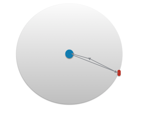
We conclude this Section discussing some interesting properties of (16). Tensor 3-point functions satisfying the stationarity condition (15) do not necessarily suffer from decorrelation effects as discussed in [14, 13, 15, 1]. Such effects are associated with phase decorrelations among different waves coming from several distinct causally disconnected regions, a process that tends to ‘Gaussianize’ the system for the central limit theorem. Interestingly, in our case, the delta-function conditions on the wave-vectors given in eq (15) (a consequence of stationarity) ensure us that GWs come from the same direction. This is particularly clear from eq (16), where the angular integral is carried over the single direction of propagation of the waves (see also Fig 2). The work [14] already pointed out that contributions to 3-point functions for which GW momenta are accurately aligned can avoid decorrelation effects. Our concept of stationary graviton nG singles out the category of tensor nG whose support is enhanced for such configurations, which are the only ones that can be probed by measurements of 3-point functions of GW signals.

Figure 2: The structure of the 3-point function in eq (15) requires that the three GWs entering in the correlator originate from a common direction $\hat{n}$ in the sky. In the graphical representation above, we show with the red spot the common region of emission of three GWs (which can be of cosmological origin); with the blue blob the region containing GW detectors (which can be of astrophysical size, as in the case of PTA experiments). The lines with arrows (that we intend as superimposed) indicate the GW common direction $\hat{n}$.

Besides this effect, [15] shows that GWs, in their (possibly long) way from source to detection, can collect random phases induced by long-wavelength energy fluctuations. These phases, physically associated with a Shapiro time delay effect, influence the short-wavelength GW modes propagating over cosmological distances. Indeed, they tend to suppress phase correlations of initially non-Gaussian fields, and to reduce the amplitude of connected $n$-point tensor correlation functions with $n\geq 3$. In our case, correlators depend on time differences only. Hence they are not sensitive to the entire time-travel of the wave from emission to detection, but only to the relatively short time-scale of the experiment. Although this is a more model dependent issue – depending on how long wavelength matter fluctuations influence tensor geodesics – we can develop some semi-quantitative argument as follows. The effect of long wavelength modes can be expressed in terms of coordinate redefinitions [40], which depend on time and on position. Following [15], we focus on the effect of long wavelength curvature fluctuations, and describe their effect in terms of a shift of time coordinate. We express the graviton mode in real space as

$$h_{ab}(t,\vec{x})\,=\,\sum_{\lambda}\int_{-\infty}^{\infty}df\int d^{2}\hat{n}\,e^{-2\pi\,i\,f\,\hat{n}\,\vec{x}}\,e^{2\pi\,i\,f\,\left(t+Z(t,\,\hat{n})\right)}\,{\bf e}_{ab}^{(\lambda)}(\hat{n})\,h_{\lambda}(f,\,\hat{n})\,,$$ (17)

where the function $Z(t,\hat{n})$ in the exponent (depending on time and GW direction) characterizes the effect of the long mode. In taking the equal time 3-point function in coordinate space using eq (17), and making use of stationary correlation properties as in eq (15), the $\delta$-functions in the GW directions force all the arguments of the $Z$ functions to be equal, and the $\delta$-functions in frequencies force them to cancel. The result is not dependent on time, nor on $Z$. Hence, long modes – when described as above – do not influence the equal-time 3-point function. It would be interesting to formalize this argument more precisely, but such analysis deserves more extensive work that we leave to a future publication.

3 Pulsar Timing Array overlap functions

We now investigate techniques to probe stationary tensor nG with pulsar timing arrays (from now on, PTA). Precision measurements of time delays in pulsar periods can allow astronomers to extract interesting information on the physics of the GW sector. Pulsar time delays can be due to a GW which deforming the space-time by passing between the pulsar and the earth; to intrinsic pulsar period variations; or to some unknown or less-known noise sources. By correlating measurements from distinct pulsars, noise can be reduced, and possible GW signal revealed. A correlation between different time-delay measurements lead to the concept of overlap function, which quantifies the response of a set of GW detectors to GWs with a given frequency. Starting from the overlap function, it is then possible to estimate the signal-to-noise ratio associated to dedicated GW observables aimed at characterise the non-Gaussian properties of a SGWB. In this Section, after reviewing in Section 3.1 well known results on 2-point overlap functions for PTA observations, we pass to discuss 3-point functions specializing to the case of stationary graviton non-Gaussianity. In particular:

1. In Section 3.2 we discuss overlap functions for pulsar timing arrays designed to probe tensor non-Gaussianity with folded shapes, corresponding to stationary graviton non-Gaussianity (see Section 2). When correlating GW measurements from PTA experiments we expect the signals to have comparable frequencies. Hence we probe flattened triangle shapes with comparable side lengths in momentum space, corresponding to the right panel of Fig 1.

2. The tensor bispectrum can correlate also modes with different spins (e.g. tensors with scalars). This might lead to interesting observables when investigating theories of modified gravity with extra degrees of freedom (as in scalar-tensor theories). For the first time, in Section 3.3 we compute mixed 3-point overlap functions for GW experiments correlating tensor and scalar fluctuations, specialising to the case of PTA experiments.

3. A stationary tensor 3-point function can also correlate GWs with very distinct frequencies, as long as they satisfy the $\delta$-function constraints of eq (15): an example is the flattened triangle in momentum space of Fig 1 (left panel) in which one of the frequencies is much smaller than the others. This implies that triangle configurations can be probed by correlating different experiments operating over different frequency ranges. For the first time, in Section 3.4 we build overlap functions correlating distinct experiments: PTA (detecting SGWBs at frequencies of order $f_{\rm PTA}\,\sim\,10^{-9}-10^{-7}$ Hz) and ground based detectors (operating at frequencies of $f_{\rm GB}\,\sim\,10^{0}-10^{3}$ Hz).

Following the review in [2], we define the total time-delay output $s_{\alpha}$ measured by a GW experiment based on a PTA system as sum of a GW signal $\sigma_{\alpha}$, and the noise $n_{a}$. We assume that the noise is uncorrelated with the GW signal, and both have average zero. For any GW propagating in the direction $\hat{n}$, we define the signal detected by the PTA in terms of the relative time delay induced by the GW on the pulsar period

$$\sigma_{\alpha}(t)\,\equiv\,\frac{\Delta T_{\alpha}}{T_{\alpha}}\,=\,\frac{x_{\alpha}^{i}\,x_{\alpha}^{j}}{2(1+\hat{n}\cdot\hat{x}_{\alpha})}\,\left[h_{ij}(t,\,\vec{x}=0)-h_{ij}(t-\tau_{\alpha},\,\vec{x}_{\alpha})\right]\,,$$ (18)

where the Earth is located at position $\vec{x}\,=\,0$, while the pulsar $\alpha$ is located at position $\vec{x}\,=\,\vec{x}_{\alpha}$. $\tau_{\alpha}$ is the light travel time from the pulsar to the Earth and $\hat{x}_{a}$ the unit vector between the Earth and the pulsar position. Expressing this quantity in Fourier space, we find

$$\sigma_{\alpha}(t)\,=\,\sum_{\lambda}\int_{-\infty}^{\infty}df\int d^{2}\hat{n}\ F^{(\lambda)}_{\alpha}(\hat{n})\,e^{2\pi\,i\,f\,t}\,h_{\lambda}(f,\,\hat{n})\,\left(1-e^{-2\pi if\tau_{\alpha}}\,e^{-2\pi\,i\,f\,\hat{n}\,\vec{x}_{\alpha}}\right)\,,$$ (19)

where we introduce the detector tensor

$$F_{\alpha}^{(\lambda)}(\hat{n})\,=\,\frac{x_{\alpha}^{i}\,x_{\alpha}^{j}\,{\bf e}_{ij}^{(\lambda)}(\hat{n})}{2(1+\hat{n}\cdot\hat{x}_{\alpha})}\,\,,$$ (20)

which depends only on the GW direction, but not on the GW frequency $f$.

3.1 Two-point overlap functions

The simplest possibility to consider is the 2-point correlation function. We review this well known case here, before discussing new results for the 3-point overlap function for stationary nG. The 2-point function for the GW modes is given in eq (14). The equal-time 2-point correlation function for the PTA time-delay signal reads

$$\langle\sigma_{\alpha}(t)\sigma_{\beta}(t)\rangle = \sum_{\lambda_{1}\lambda_{2}}\int_{-\infty}^{\infty}df_{1}df_{2}\int d^{2}\hat{n}_{1}d^{2}\hat{n}_{2}\ F^{(\lambda_{1})}_{\alpha}(\hat{n}_{1})F^{(\lambda_{2})}_{\beta}(\hat{n}_{2})\,e^{2\pi\,i\,\left(f_{1}+f_{2}\right)\,t}\,P(f_{1})$$

$$\times\,\,\delta^{(2)}(\hat{n}_{1}-\hat{n}_{2})\,\delta(f_{1}+f_{2})\,\delta_{\lambda_{1}\lambda_{2}}\,\left(1-e^{-2\pi if_{1}\tau_{\alpha}\left(1+\hat{n}_{1}\,\hat{n}_{\alpha}\right)}\right)\,\left(1-e^{-2\pi if_{2}\tau_{\beta}\left(1+\hat{n}_{2}\,\hat{n}_{\beta}\right)}\right)\,.$$

For pulsars at typical distances of $10^{3}$ parsec, taking into account the frequency range probed by PTA, one finds that the quantity $f\tau_{\alpha}\sim{\cal O}(10^{2})$. This implies that contributions containing exponentials in the pulsar terms, in the second line of the previous equation, are rapidly oscillating functions that are averaged out in the integral over directions $\hat{n}$. Hence we can neglect these terms and substitute the second line with a unit factor.

Figure 3: Representation of a system of two pulsars, and the earth. We denote with $\zeta$ the angle between the unit vectors from the earth towards each of the pulsars.

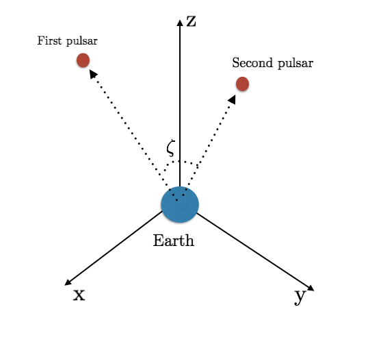
Under this approximation, making use of the $\delta$ functions, we can assemble the angular integral into a response function, and express the previous quantity as

$$\langle\sigma_{\alpha}(t)\sigma_{b}(t)\rangle = 2\pi\,\sum_{\lambda}\int df\,{\cal R}^{(\lambda)}_{\alpha\beta}\,P(f)\,,$$ (22)

where the PTA 2pt response function is given by an angular integration, leading to the so-called Hellings-Down overlap function [25] (see also [26, 41, 2]):

$${\cal R}^{(\lambda)}_{\alpha\beta}(\zeta) = \int\frac{d^{2}\hat{n}}{2\pi}\,F^{(\lambda)}_{\alpha}(\hat{n})F^{(\lambda)}_{\beta}(\hat{n})\,,$$ (23)

$$= \frac{1}{6}-\frac{\left(1-\cos\zeta\right)}{24}\left(1-6\,\ln\left(\frac{1-\cos\zeta}{2}\right)\right)\,,$$ (24)

where

$$\cos\zeta\,\equiv\,\hat{x}_{\alpha}\,\cdot\,\hat{x}_{\beta}\,.$$ (25)

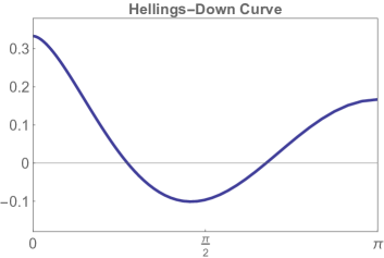
It is important to stress that the Hellings-Down function ${\cal R}^{(\lambda)}_{\alpha\beta}$ depends only on angle $\zeta$ between pulsar directions, and not on the GW frequency. In Fig 4 we represent the profile of the sum of overlap functions over polarization indexes, ${\cal R}_{\alpha\beta}(\zeta)\,=\,\sum_{\lambda}{\cal R}^{(\lambda)}_{\alpha\beta}$.

Figure 4: The 2-point overlap function for the sum of the spin-2 polarizations ${\cal R}_{ab}(\zeta)\,=\,\sum_{\lambda}{\cal R}^{(\lambda)}_{ab}$ (the so-called Hellings-Down curve [25]). The $x$-axis contain the angle $\zeta$ defined in eq (25). The $y$-axis the corresponding value of the overlap function, see eq (23).

3.2 Three-point overlap functions

We now analyze the 3-point overlap function for flattend tensor bispectra satisfying a stationarity condition, as described in Section 2. Such shapes of tensor bispectra were not specifically investigated in [29], hence our results are new. In correlating signals from different pulsars, we assume that the frequencies of the GWs are comparable, hence the flattened tensor bispectra in momentum space have a shape with sides of similar size, see the right panel of Fig 1.

The tensor 3-point function in Fourier space is given by eq (15). The PTA signal equal-time 3pt function then results, using the notation of the previous subsection, is

$$\langle\sigma_{\alpha}(t)\sigma_{\beta}(t)\sigma_{\gamma}(t)\rangle = \sum_{\lambda_{1}\lambda_{2}\lambda_{3}}\int_{-\infty}^{\infty}df_{1}df_{2}\int d^{2}\hat{n}\,F^{(\lambda_{1})}_{\alpha}(\hat{n})F^{(\lambda_{2})}_{\beta}(\hat{n})F^{(\lambda_{3})}_{\gamma}(\hat{n})\,{B}^{\lambda_{1}\lambda_{2}\lambda_{3}}(f_{1},f_{2},\hat{n}_{\star})\,.$$

We now conveniently collect the angular integration in the definition of the 3-point overlap function ${\cal R}_{\alpha\beta\gamma}^{\lambda_{1}\lambda_{2}\lambda_{3}}(\hat{n}_{\star})$:

$$\langle\sigma_{\alpha}(t)\sigma_{\beta}(t)\sigma_{\gamma}(t)\rangle = \sum_{\lambda_{1}\lambda_{2}\lambda_{3}}2\pi\,\int_{-\infty}^{\infty}df_{1}df_{2}\,{\cal R}_{\alpha\beta\gamma}^{\lambda_{1}\lambda_{2}\lambda_{3}}(\hat{n}_{\star})\,{B}^{\lambda_{1}\lambda_{2}\lambda_{3}}(f_{1},f_{2},\hat{n}_{\star})\,.$$ (27)

To perform such angular integrations, we introduce a rotation matrix $M\left[\theta,\,\phi\right]$:

$$M\left[\theta,\,\phi\right]=\left(\begin{array}[]{ccc}\sin\theta\cos\phi&\cos\theta\cos\phi&-\sin\phi\\ \sin\theta\sin\phi&\cos\theta\sin\phi&\cos\phi\\ \cos\theta&-\sin\theta&0\end{array}\right)\,.$$ (28)

We rotate over the reference direction $n_{\star}$: $\hat{n}\,=\,M\left[\theta,\,\phi\right]\,\hat{n}_{\star}$, so to write

$${\cal R}^{\lambda_{1}\lambda_{2}\lambda_{3}}_{\alpha\beta\gamma}(\hat{n}_{\star})\,=\,\frac{1}{2\pi}\int_{0}^{2\pi}\,d\phi\,\,\int_{0}^{\pi}\,\sin{\theta}\,d\theta\,\left[F^{(\lambda_{1})}_{\alpha}(M\,\hat{n}_{\star})F^{(\lambda_{2})}_{\beta}(M\,\hat{n}_{\star})F^{(\lambda_{3})}_{\gamma}(M\,\hat{n}_{\star})+\left(\lambda_{i}\to-\lambda_{i}\right)\right]\,.$$ (29)

Notice that the PTA 3-point overlap function depends on the chirality of the GW, the relative position of pulsars, and the reference direction $\hat{n}_{\star}$. From now on, in this work we select $\hat{n}_{\star}$ to point along the $\hat{x}$ axis:

$$\hat{n}_{\star}\,=\,\left(1,\,0,\,0\right)\,.$$ (30)

On the other hand, the overlap function does not depend on the frequency since (for the same arguments discussed in Section 3.1) we can safely neglect the earth terms. In what follows, we do not consider scenarios including parity violation, and we sum over opposite chiralities. In other words, indicating $R\,=\,+$ and $L\,=\,-$, we compute and plot the sum ${\cal R}^{\lambda_{1}\lambda_{2}\lambda_{3}}_{\alpha\beta\gamma}+{\cal R}^{-\lambda_{1}\,-\lambda_{2}\,-\lambda_{3}}_{\alpha\beta\gamma}$, as done in Section 3.1 for the 2-point overlap function.

Evaluating the precise angular structure of ${\cal R}^{\lambda_{1}\lambda_{2}\lambda_{3}}_{\alpha\beta\gamma}(\hat{n}_{\star})$ is essential for estimating the optimal signal-to-noise ratio of an experiment to measure a stationary tensor bispectrum, as we shall learn in Section 4. In the next two subsections, we evaluate the 3-point overlap functions in two different configurations.

3.2.1 3-point overlap function: two signals from the same pulsar

In this subsection we compute the overlap function for a case where we correlate two time-delay signals from the same pulsar $\alpha$, with a third signal from a separate pulsar $\beta$. This case will be important for the discussion in Section 4. We consider the limit of equal time 3-point correlation

$$\left\langle\sigma_{\alpha}\left(t\right)\sigma_{\alpha}\left(t\right)\sigma_{\beta}\left(t\right)\right\rangle\,,$$ (31)

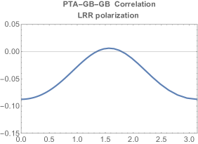
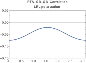
and we represent in Fig 5 for a graphical representation of the geometry of the system.

Figure 5: Representation of a configuration where we correlate two signals measured at the same pulsar $\alpha$ with a signal for the distinct pulsar $\beta$.

In this case we find that the 3-point overlap function depends only on the angle $\zeta$ between the vectors from the earth towards pulsars $\alpha$ and $\beta$. The general formula to compute such function is given by eq (29), with $\gamma=\beta$. The response function ${\cal R}_{\alpha\beta\beta}^{\lambda_{1}\lambda_{2}\lambda_{3}}$ depends on chirality, see Fig 6. Its magnitude is around few percent, depending on the value of $\zeta$. We find ${\cal R}_{\alpha\beta\beta}^{RRR}\,=\,{\cal R}_{\alpha\beta\beta}^{RLR}$. Notice that these results are quite different from the Hellings-Down profile reviewed in Section 3.1 for the 2-point function, in respect of size and angular profile.

Figure 6: 3-point overlap functions associated with stationary, flattened bispectra, for correlating two signals from the same pulsar with a signal from another pulsar (see Fig 5). In the x-axis we vary the angle $\zeta$ between the unit vectors from the earth towards pulsars $\alpha$ and $\beta$. In the y-axis we represent the magnitude of the associated 3-point function, which depends on the polarization of the GWs.

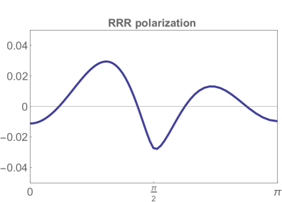
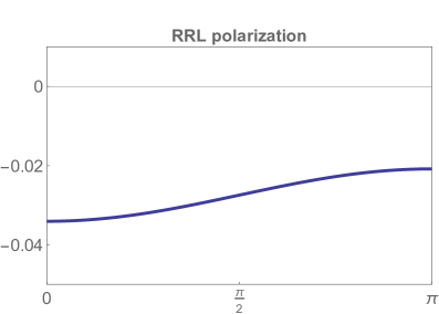
3.2.2 3-point overlap function: signals from from three distinct pulsars

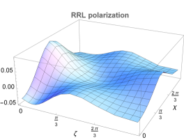
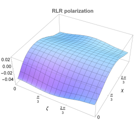
When we correlate time-delay signals from three different pulsars, the result depends in a more complex way on the geometry of the system. For definiteness, here we focus our attention on a system where the three pulsars lie on orthogonal planes, $(x,\,y)$, $(x,\,z)$, $(y,\,z)$: see Fig 7.

Figure 7: A configuration with three pulsars lying on orthogonal planes. In this representative figure, $\zeta$ denotes the angle beween the unit vectors from the earth towards pulsar 1 and 2. $\chi$ denotes the angle beween the unit vectors from the earth towards pulsar 2 and 3.

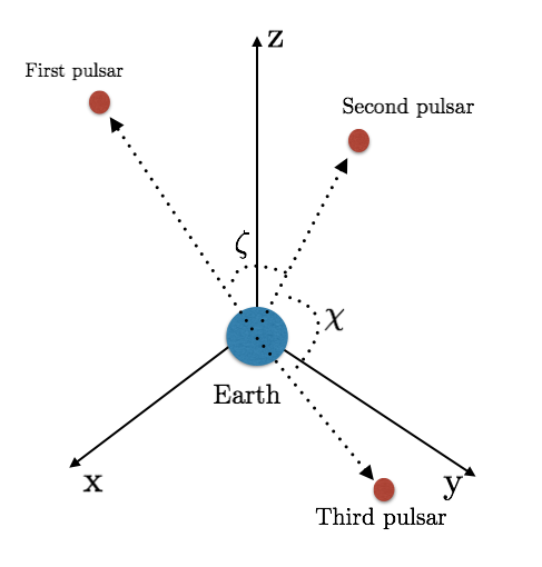
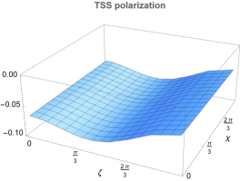
In this case, the 3-point overlap function depends on two angles $\zeta$ and $\chi$ between the vectors from earth towards the pulsars. We represent our results for the overlap functions in Fig 8, evaluated using the general formula (29). Also in this case the typical magnitude of the overlap function is of order of a few percent. On the other hand, the plots in Fig 8 also present peaks and valleys where the magnitude of the overlap function can increase by a factor of order one with respect to the 2-dimensional case studied in section 3.2.1.

Figure 8: Three-point overlap functions associated with stationary, flattened bispectra We locate the pulsars in three different orthogonal planes (say (xy), (yz), (xz)) and vary the angle $\zeta$ between the unit vectors from the earth towards pulsar 1 and 2, and $\chi$ the unit vectors from the earth towards pulsar 1 and 3. The z-axis represents the magnitude of the corresponding overlap function.

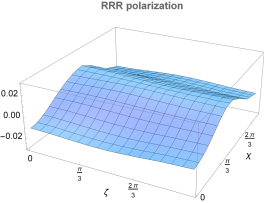
3.3 Three-point overlap functions: correlating tensor and scalar polarizations

GW experiments can be sensitive also to vector and scalar polarizations of GWs, motivated by theories that modify General Relativity: see the interesting early works [42, 43] that first explored this possibility, and [30, 31, 32] for analysis that specifically cover PTA experiments. GW 2-point functions do not correlate fields of different spin (e.g. scalar and tensors) around an isotropic background; instead, correlations among different spins are possible at the level of 3-point functions. In this subsection, for the first time we investigate 3-point overlap functions describing the correlation of scalar GW polarizations with tensor (or scalar) polarizations. Our results are model independent, and we do not refer to specific scenarios. But, for the same reasons discussed in the previous sections, we focus on stationary non-Gaussianity, associated with time-translation-invariant 3-point functions (that is, bispectra with folded shapes in momentum space). Our conventions for polarization tensors describing the transverse scalar ‘breathing mode’ GW polarization are standard and listed in Appendix A.

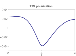
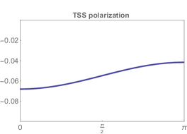
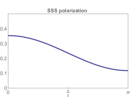
We first consider correlation of two signals from the same pulsar $\alpha$ with a signal from a distinct pulsar $\beta$, as in subsection 3.2.1. Figure 9 shows our result for the overlap function relative to a stationary bispectrum of folded shape, with correlate scalar and tensor modes. Interestingly, the magnitude of the overlap function in the presence of scalar excitations is larger than in the case of spin-2 modes only, and does not depend on the chirality (L/R) of tensors entering the correlators. As we shall see, this fact has some consequences in the computation of the signal-to-noise ratio.

Figure 9: Three-point overlap functions correlating two signals from the same pulsar $\alpha$ with a signal from second pulsar $\beta$. We vary the angle $\zeta$ between the unit vectors from the earth towards pulsar a and b. We correlate tensor T polarization with scalar S polarization.

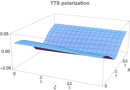
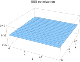
We then consider correlation of three signals from three distinct pulsars, with the condition that the three pulsars lie on orthogonal planes, as done in Section 3.2.2 in a purely tensor context. Figure 10 shows our results for the overlap functions for this case. Notice that for the pulsar configuration we consider the overlap function for scalar autocorrelations is flat.

Figure 10: Three-point overlap functions correlating scalar and tensor modes for signals from three different pulsars lying on orthogonal planes. We vary the angle $\zeta$, $\chi$ between the unit vectors from the earth towards the pulsars. We correlate tensor (T) polarization with scalar (S) polarization.

3.4 Three-point overlap functions: correlating PTA and ground-based experiments

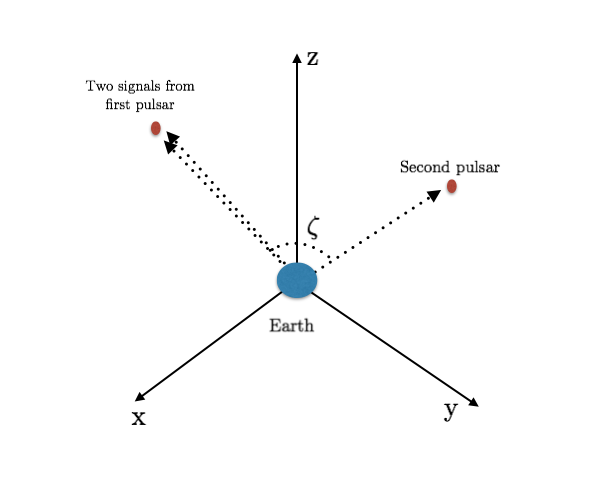
Another interesting feature of stationary tensor nG is the possibility to correlate signals with very different frequencies, associated with triangles in momentum space for which one of the side lengths is much smaller than the other two (see Fig 1, left panel). In cases in which the frequencies involved differ by several orders of magnitude, it is interesting to correlate signals detected by PTA experiments with signals measured by ground-based experiments (e.g. LIGO) that work in the frequency range $10^{0}-10^{3}$ Hz. See Figure 11 for a graphical representation of the system.

Figure 11: Representation of a possible measurement where we correlate signals measured with PTA with signals detected with ground-based experiments (labelled as ‘LIGO’).

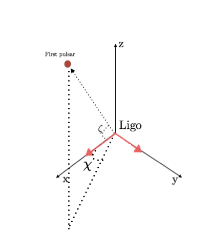
The calculation of the corresponding overlap function is conceptually similar to what we have done so far: only the expression for the detector tensor (given in eq (20) for the PTA case) changes. In the small-antenna limit, the detector tensor for ground based experiments reads:

$$F_{\alpha}^{(\lambda)}(\hat{n})\,=\,\frac{1}{2}\,{\bf e}_{ij}^{(\lambda)}\left(X_{a}^{i}\,X_{a}^{j}-Y_{a}^{i}\,Y_{a}^{j}\right)\,,$$ (32)

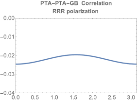
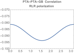
with $\vec{X}_{a}$, $\vec{Y}_{a}$ indicating the arm directions of the interferometer $\alpha$. It is sufficient to plug this expression for the detector tensor in the general formula (29) for the 3-point detector function to study the case of cross correlations among different experiments. We represent our results in Figs 12 and 13. In Fig 12, we correlate two signals from the same pulsar with a signal measured by a ground-based detector.

Figure 12: 3-point overlap functions for correlations between two signals from the same pulsar and a signal measured at a ground-based detector. We vary the angle $\zeta$ between the unit vectors from the earth and a direction of one of the ground based detector arms.

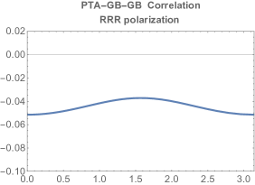
In Fig 13, instead, we correlate one signal from a pulsar with two signals measured by the same ground based detector.

Figure 13: 3-point overlap functions for correlations between one signal from a pulsar and two signals measured at the same ground-based detector. We vary the angle $\zeta$ between the unit vectors from the earth and a direction of one of the ground based detector arms.

4 The optimal signal-to-noise ratio for stationary tensor nG

Armed with the results of Section 3 on the PTA overlap functions, we now wish to determine the optimal way to correlate measurements from different pulsars, so to maximise the signal-to-noise ratio (SNR) when measuring stationary tensor bispectra in flattened configurations with Pulsar Timing Arrays. We call $s_{\alpha}(t)$ the output of the measurement at time $t$ from pulsar $\alpha$, which is the sum of GW signal $\sigma_{\alpha}(t)$ and noise $n(t)$. (And same for pulsars $\beta$, $\gamma$.) In order to carry on our computations, we make the following assumptions:

• We shall assume that the noise dominates over the GW signal. The total time $T$ during which data are collected ($5$-$10$ years) is much larger than the typical frequency scale of the detected GWs (say $f\sim 10$ nHz), so we work in a regime $fT\gg 1$.

• We will assume that the graviton bispectrum is very peaked in flattened configurations as described in Section 2, so that the condition of stationary bispectrum is very well realised, and any variance associated with the spread of the bispectrum shape is well smaller than the (dominant) instrumental noise as discussed in the previous bullet point. It would be interesting to study concrete early universe models leading to graviton nG with this property, but we leave this for future work.

Under these hypothesis, we start deriving the expression for the optimal signal-to-noise ratio, which (as we shall see) depends on the frequency dependence of the tensor bispectrum, as we well as a constant geometrical quantity that we call ${\texttt{r}}^{\lambda_{1}\lambda_{2}\lambda_{3}}$ ($\lambda_{i}$ denoting the GW chirality). The quantity ${\texttt{r}}^{\lambda_{1}\lambda_{2}\lambda_{3}}$ depends on the GW chirality and on the number and geometrical configuration of the pulsars in the PTA system under consideration. Towards the end of the section, we shall collect in a table the values for this quantity, when evaluated for the IPTA data set [23].

In order to estimate the optimal SNR, we generalise to the case of 3-point functions the methods described in the textbook [44] and the articles [26, 45]. The computation of the optimal SNR for tensor bispectrum has been already carried on in [7]: here we simplify the analysis by adapting the computation to the present context, where we focus on ‘stationary’ non-Gaussianity only, and on PTA measurements. We define the stationary three point correlator among a measurement performed with a triplet of pulsars, denoted with $(\alpha,\,\beta,\,\gamma)$:

$${\cal Y}_{\alpha\beta\gamma}\,=\,\int_{-T/2}^{T/2}\,dt_{1}\int_{-T/2}^{T/2}\,dt_{2}\int_{-T/2}^{T/2}\,dt_{3}\,s_{\alpha}(t_{1})s_{\beta}(t_{2})s_{\gamma}(t_{3})\,Q(t_{3}-t_{1})\,Q(t_{3}-t_{2})\,,$$ (33)

where we integrate over the duration $T$ of the experiment. In the previous expression, $Q(t_{i}-t_{j})$ is a filter function, depending on time differences, which we assume decays very rapidly with increasing values of $|t_{i}-t_{j}|$. Notice that we include two copies of $Q$, in order to take into account the two independent time differences $(t_{3}-t_{1})$ and $(t_{2}-t_{1})$.

In the definition of SNR$\equiv$S$/$N, the quantity S (the signal) corresponds to the ensemble average value of ${\cal Y}_{\alpha\beta\gamma}$ when the signal is present; the quantity N (the noise) is the root mean square value of ${\cal Y}_{\alpha\beta\gamma}$ when the signal is absent. In what comes next, we wish to determine the choice of filter function $Q$ maximising the SNR.

We Fourier transform the expression (33):

$${\cal Y}_{\alpha\beta\gamma} = \int_{-\infty}^{\infty}\,df_{A}\,df_{B}\,df_{1}\,df_{2}\,df_{3}\,\,\delta_{T}(f_{1}-f_{A})\,\delta_{T}(f_{2}-f_{B})\,\delta_{T}(f_{3}+f_{A}+f_{B})$$ (34)

$$\times\,\tilde{s}_{\alpha}(f_{1})\,\tilde{s}_{\beta}(f_{2})\,\tilde{s}_{\gamma}(f_{3})\,\tilde{Q}(f_{A})\,\tilde{Q}(f_{B})\,,$$

and introduce the function $\delta_{T}(f)\,\equiv\,\left(\int_{-T/2}^{T/2}\,dt\,\exp{2\pi\,i\,ft}\right)$. This function approaches the Dirac delta function for $T\to\infty$, and has the property that $\delta_{T}(0)\,=\,T$. We proceed integrating over the frequencies $f_{1}$, $f_{2}$. We get (in the physically relevant limit of large $f\,T$ where we can approximate $\delta_{T}$ with a $\delta$ function):

$${\cal Y}_{\alpha\beta\gamma} = \int_{-\infty}^{\infty}\,df_{A}\,df_{B}\,df_{3}\,\,\delta_{T}(f_{3}+f_{A}+f_{B})\,\tilde{s}_{\alpha}(f_{A})\,\tilde{s}_{\beta}(f_{B})\,\tilde{s}_{\gamma}(f_{3})\,\tilde{Q}(f_{A})\,\tilde{Q}(f_{B})\,.$$ (35)

We now compute the SNR$\equiv$S$/$N.

The signal S. Using the procedure outlined above, and equation (19) for the individual signals from each pulsar, we get the following expression for the total signal associated with the 3-pulsar measurement:

$$S = \sum_{\lambda_{1}\lambda_{2}\lambda_{3}}\int_{-\infty}^{\infty}\,df_{A}\,df_{B}\,df_{3}\,d^{2}\hat{n}_{1}\,d^{2}\hat{n}_{2}\,d^{2}\hat{n}_{3}\,\delta_{T}(f_{3}+f_{A}+f_{B})\,F_{\alpha}^{\lambda_{1}}(\hat{n}_{1})\,F_{\beta}^{\lambda_{2}}(\hat{n}_{2})\,F_{\gamma}^{\lambda_{3}}(\hat{n}_{3})$$ (37)

$$\times\,\langle h_{\lambda_{1}}(f_{A},\hat{n}_{1})\,h_{\lambda_{2}}(f_{B},\hat{n}_{2})\,h_{\lambda_{3}}(f_{3},\hat{n}_{3})\rangle\,\tilde{Q}(f_{A})\,\tilde{Q}(f_{B})\,,$$

$$= \sum_{\lambda_{1}\lambda_{2}\lambda_{3}}\,\int_{-\infty}^{\infty}\,df_{A}\,df_{B}\,df_{3}\,\delta(f_{3}+f_{A}+f_{B})\,\delta_{T}(f_{3}+f_{A}+f_{B})\,,$$

$$\,\tilde{Q}(f_{A})\,\tilde{Q}(f_{B})\,{B}^{\lambda_{1}\lambda_{2}\lambda_{3}}(f_{A},f_{B},\,\hat{n}_{\star})\,{\cal R}_{\alpha\beta\gamma}^{\lambda_{1}\lambda_{2}\lambda_{3}}(\hat{n}_{\star})\,,$$

$$= T\,\sum_{\lambda_{1}\lambda_{2}\lambda_{3}}\,\int_{-\infty}^{\infty}\,df_{A}\,df_{B}\,,\,\tilde{Q}(f_{A})\,\tilde{Q}(f_{B})\,{B}^{\lambda_{1}\lambda_{2}\lambda_{3}}(f_{A},f_{B},\,\hat{n}_{\star})\,{\cal R}_{\alpha\beta\gamma}^{\lambda_{1}\lambda_{2}\lambda_{3}}(\hat{n}_{\star})\,,$$ (38)

where we use the fact that $\delta_{T}(0)=T$, and make use of expression (15) for the GW three point function in momentum space.

The noise N. We assume that the noise is Gaussian and uncorrelated between pulsars; we define the noise spectrum as

$$\langle n_{\alpha}(f_{A})n_{\alpha}^{*}(f_{C})\rangle\,=\,S_{n}\,\delta(f_{A}-f_{C})\,,$$ (39)

where we use the fact that PTA noise is frequency independent. We make use of the following formula from [45]:

$$S_{n}\,=\,2\Delta t\,\sigma^{2}\,,$$ (40)

with $1/\Delta t$ the measurement cadence (of order $20$ yr^-1), and $\sigma^{2}$ the rms of the noise timing (for IPTA pulsars, this quantity is of order $1$ $\mu$s). The noise squared of the measurement, in absence of signal, is

$$N^{2} = \langle{\cal Y}{\cal Y}^{*}\rangle\,,$$ (42)

$$= \int df_{A}\,df_{B}\,df_{3}\,df_{C}\,df_{D}\,df_{4}\,\,\delta_{T}(f_{3}+f_{A}+f_{B})\,\delta_{T}(f_{4}+f_{C}+f_{D})$$

$$\times\langle n_{\alpha}(f_{A})n_{\alpha}^{*}(f_{C})\rangle\langle n_{\beta}(f_{B})n_{\beta}^{*}(f_{D})\rangle\langle n_{\gamma}(f_{3})n_{\gamma}^{*}(f_{4})\rangle$$

$$\times Q(f_{A})Q^{*}(f_{C})Q(f_{B})Q^{*}(f_{D})\,,$$

$$= T\,S_{n}^{3}\,\int df_{A}\,df_{B}\,|Q(f_{A})|^{2}\,|Q(f_{B})|^{2}\,\,.$$ (43)

Then the ratio corresponding to signal-to-noise is the ratio of the quantity $S$ in eq (38) versus $N$ of eq (43). We can sum over all the available distinct pulsar triplets $(\alpha,\,\beta,\,\gamma)$ in the network under consideration . We find

$$\text{SNR}\,=\,\sqrt{T}\,\frac{\left[\sum_{\alpha\beta\gamma}\sum_{\lambda_{i}}\int_{-\infty}^{\infty}\,df_{A}\,df_{B}\,\,\tilde{Q}(f_{A})\,\tilde{Q}(f_{B})\,\left(\,{B}^{\lambda_{1}\lambda_{2}\lambda_{3}}(f_{A},f_{B},\,\hat{n}_{\star})\,{\cal R}_{\alpha\beta\gamma}^{\lambda_{1}\lambda_{2}\lambda_{3}}(\hat{n}_{\star})\right)\right]}{\left[\,S_{n}^{3}\,\int df_{A}\,df_{B}\,|Q(f_{A})|^{2}\,|Q(f_{B})|^{2}\,\right]^{1/2}}\,.$$ (44)

In order to determine the function $Q$ maximising the previous expression, we first define a positive definite scalar product $[\cdots,\cdots]$ between two quantities which depend on frequency (recall that $S_{n}$ is a positive quantity):

$$\left[A_{1}(f_{a},f_{b}),\,A_{1}(f_{a},f_{b})\right]\,=\,\int df_{a}\,df_{b}\,\,A_{1}(f_{a},f_{b})\,A_{2}^{*}(f_{a},f_{b})\,S_{n}^{3}\,.$$ (45)

By dropping indexes, the SNR of eq (44) can be then schematically re-expressed in terms of this scalar product as

$$\text{SNR}\,=\,\sqrt{T}\,\frac{\left[QQ,\,{B}\,{\cal R}/S_{n}^{3}\right]}{\left[QQ,\,QQ\right]^{1/2}}\,.$$ (46)

The previous quantity is maximized by choosing the function $Q$ as

$$Q(f_{a})Q(f_{b})\,=\,\frac{{B}(f_{a},f_{b},\,n^{*})\,{\cal R}(n^{*})}{S_{n}^{3}}\,.$$ (47)

To summarize, the optimal SNR is given by the expression

$$\text{SNR}_{\text{opt}}\,=\,\sqrt{4\,T}\,\left[\sum_{\lambda_{1}\lambda_{2}\lambda_{3}}\,\frac{\int_{0}^{\infty}\,df_{A}\,df_{B}\left({\texttt{r}}^{\lambda_{1}\lambda_{2}\lambda_{3}}\,{B}^{\lambda_{1}\lambda_{2}\lambda_{3}}(f_{A},f_{B},\,\hat{n}_{\star})\,\right)^{2}}{S_{n}^{3}}\right]^{\frac{1}{2}}\,,$$ (48)

where we find convenient to define a single quantity ${\texttt{r}}^{\lambda_{1}\lambda_{2}\lambda_{3}}$ containing the sum of the PTA response functions over all independent pulsar triplets:

$${\texttt{r}}^{\lambda_{1}\lambda_{2}\lambda_{3}}\,=\,\left[\sum_{\alpha\beta\gamma}\left({\cal R}_{\alpha\beta\gamma}^{\lambda_{1}\lambda_{2}\lambda_{3}}(\hat{n}_{\star})\right)^{2}\right]^{\frac{1}{2}}\,.$$ (49)

	Case 1	Case 2
${\texttt{r}}^{RRR}$	$20.17$	$0.58$
${\texttt{r}}^{RRL}$	$19.58$	$0.99$
${\texttt{r}}^{RLR}$	$19.58$	$0.99$
${\texttt{r}}^{STT}$	$38.11$	$0.28$
${\texttt{r}}^{SST}$	$119.49$	$1.96$
${\texttt{r}}^{SSS}$	$168.99$	$9.12$

Table 1: Value of the quantity ${\texttt{r}}^{\lambda_{1}\lambda_{2}\lambda_{3}}$ for different GW tensor polarizations, computed for two different cases using IPTA data. Case 1: we do the sum of eq (49) summing over distinct pulsar triplets. Case 2: the sum is made assuming that we correlate two signals from one pulsar with one signal from another pulsar (as in Section 3.2.1) hence we sum over distinct couples of pulsars. We consider purely tensor correlators (depending on chirality, upper part of the table) and scalar-tensor correlators (lower part of the table).

Hence we learn that the optimal SNR, besides than on the frequency dependence of the bispectrum, is characterized by the constant quantity ${\texttt{r}}^{\lambda_{1}\lambda_{2}\lambda_{3}}$ of eq. (49). This depends on the GW polarization, and on the number and position of the pulsars one considers. We compute this quantity for the case of IPTA pulsars – an international collaboration monitoring the period of 49 pulsars from different PTA data set, see Appendix B – in Table 1. Summing over distinct triplets of pulsars (Case 1) give much larger values for the parameter $r^{\lambda_{1}\lambda_{2}\lambda_{3}}$, than summing over couples (Case 2): we believe that this is due to the large number of independent triples one can form with the large pulsar data set we use. Also, both for Case 1 and 2, the size of this parameter is much larger in the case of correlations involving scalar modes only, since the corresponding overlap function is one order of magnitude larger than in the case of tensor correlators, see Section 3.

Our conclusion is that the optimal SNR for measuring stationary graviton non-Gaussianity can be greatly enhanced by monitoring larger numbers of pulsars, since it depends on number and configurations of pulsar triplets. It will be interesting to build explicit models leading to stationary tensor nG, and investigate at what extent we can probe amplitude and slope (i.e. frequency dependence) of a stationary tensor bispectrum with current (IPTA) and future (SKA) PTA experiments. We leave these investigations to future work.

5 Conclusions

In this work we introduced the concept of stationary graviton non-Gaussianity (nG). We discussed how its properties make it the only type of graviton nG that can be directly measurable in terms of three-point functions of a stochastic gravitational wave background (SGWB). When evaluated in Fourier space, 3-point functions associated with stationary nG correspond to configurations peaked in folded configurations. We determined 3-point overlap functions for probing stationary nG with PTA experiments, and we obtained the corresponding optimal signal-to-noise ratio (SNR). For the first time, we considered 3-point overlap functions for PTA including scalar graviton polarizations (which can be motivated in theories of modified gravity); moreover, we also calculated 3-point overlap functions for correlating PTA with ground based GW interferometers. We have shown that the value of the optimal SNR depends on the number and position of monitored pulsars. We built geometrical quantities characterizing how the SNR depends on the PTA system under consideration, and we evaluated such geometrical parameters using data from the IPTA collaboration. We shown that monitoring a large number of pulsars can increase the SNR associated with measurements of stationary graviton nG.

If in the future a SGWB will be detected with PTA GW experiments, it will be interesting to try to measure the corresponding signal 3-point function with the tools we developed here. If data will provide evidence for stationary nG, a challenge for theorists will be to design and characterize early universe scenarios (possibly using approaches based on the effective field theory of inflation) able to realize folded configurations for graviton nG in momentum space.

Acknowledgments

Is is a pleasure to thank Enrico Barausse, Nicola Bartolo, Valerio De Luca, Emanuela Dimastrogiovanni, Matteo Fasiello, Gabriele Franciolini, Marco Peloso, and Toni Riotto for useful discussions and suggestions, and for comments on a draft of this work. G.T. is partially supported by STFC grant ST/P00055X/1.

Appendix A Conventions for the polarization tensors

We adopt standard conventions for the polarization tensors adapted to the GW direction $\hat{n}$, the same used in [7]. We assume a Cartesian coordinate system with orthogonal axis $(\hat{x},\,\hat{y},\,\hat{z})$. Starting from the GW direction $\hat{n}$ we define two orthogonal unit vectors $\hat{u}$ and $\hat{v}$:

$$\hat{u} = \frac{\hat{n}\times\hat{z}}{|\hat{n}\times\hat{z}|}\hskip 28.45274pt,\hskip 28.45274pt\hat{v}\,=\,\hat{n}\times\hat{u}\,.$$ (50)

Using these unit vectors, we can define two tensor polarizations $(+,\,\times)$:

$$e^{(+)}_{ab} = \frac{\hat{u}_{a}\hat{u}_{b}-\hat{v}_{a}\hat{v}_{b}}{\sqrt{2}}\,,$$ (51)

$$e^{(\times)}_{ab} = \frac{\hat{u}_{a}\hat{v}_{b}+\hat{v}_{a}\hat{u}_{b}}{\sqrt{2}}\,$$ (52)

which satisy $e^{(+)}_{ab}e^{(+)}_{ab}\,=\,1\,=\,e^{(\times)}_{ab}e^{(\times)}_{ab}$, $e^{(+)}_{ab}e^{(\times)}_{ab}\,=\,0$. From these objects, we obtain the chiral polarization operators $(R,L)$ which we use in the main text:

$$e^{(R,\,L)}_{ab} = \frac{e^{(+)}_{ab}\pm i\,e^{(\times)}_{ab}}{\sqrt{2}}\,.$$ (53)

For what respect the breathing scalar mode we adopt the following polarization tensor [46]:

$$e^{(S)}_{ab} = \frac{\hat{u}_{a}\hat{u}_{b}+\hat{v}_{a}\hat{v}_{b}}{\sqrt{2}}\,.$$ (54)

Appendix B The IPTA data set

Table 2 contains data from 49 pulsars which are observed by the International Pulsar Timing Array (IPTA). The IPTA consists of various pulsar timing arrays throughout the world. This includes the Parkes Pulsar Timing Array (PPTA) in Australia, NanoGrav (consisting of Arecibo (Puerto Rico) and Green Bank Telescope (USA)) and the European Pulsar Timing Array (EPTA) (consisting of Effelsberg Radio Telescope (Germay), Nançay (France), Lovell Telescope (UK), Sardina Radio Telescope (Italy) and Synthesis Radio Telescope (Netherlands)). The combination of these various arrays allows for a larger data set of pulsars to be observed.

Pulsar Name	$\textbf{RMS}\,[\mu s]$	TOAs
J0030+0451	1.9	1,030
J0034-0538	4.4	267
J0218+4232	6.7	1,005
J0437–4715	0.3	5,052
J0610–2100	5.2	347
J0613–0200	1.2	2,940
J0621+1002	11.5	637
J0711–6830	2.0	549
J0751–6830	3.5	1,129
J0900–3144	3.4	575
J1012+5307	1.7	2,910
J1022+1001	2.2	1375
J1024–0719	5.9	918
J1045–4509	3.3	635
J1455–3330	4.0	1,495
J1600–3053	0.8	1,697
J1603–7202	2.3	483
J1640+2224	2.0	1,139
J1643–1224	2.7	2,395
J1713+0747	0.3	19,972
J1721–2457	25.5	152
J1730–2304	2.1	5.63
J1732–5049	2.5	242
J1738+0333	2.6	206
J1744–1134	1.1	2,589

Pulsar Name	$\textbf{RMS}\,[\mu s]$	TOAs
J1751–2857	2.4	78
J1801–1417	4.6	86
J1802–2124	4.3	433
J1804–2717	4.5	76
J1824–2452A	2.4	298
J1843–1113	1.7	186
J1853+1303	1.1	566
J1857+0943	1.3	1,641
J1909–3744	0.2	2,623
J1910+1256	3.0	597
J1911+1347	0.6	45
J1911–1114	5.3	81
J1918–0642	1.5	1,522
J1939+2134	70.0	3,905
J1955+2908	5.0	319
J2010–1323	1.9	296
J2019+2425	8.8	80
J2033+1734	13.3	130
J2124–3358	3.0	1115
J2129–5721	1.2	447
J2145–0750	1.2	2,347
J2229+2643	3.8	234
J2317+1439	1.6	867
J2322+2057	6.9	199

Table 2: Pulsars analyzed by IPTA [23].

J1824-2452A is followed by a letter in order to differentiate between pulsars that are in close proximity (otherwise it is difficult to give them unique names).

The pulsar names are determined by the coordinates in the sky. Pulsars with a J in front of the coordinates mean that they have more precise coordinates than older pulsars (before 1993 and these are denoted with a B). The first number is the right ascension which is the a point along the celestial equator between the sun and the March equinox to the point above the earth which is in question. This is measured in hours and minutes. The other section of the coordinates is determined by its declination which is how far above (+) or below (–) the pulsar is with respect to the celestial equator. Note that older pulsars (that begin with a B) only have their declination to the nearest degree whilst the J pulsars have more accurate coordinates.

Right ascension can be converted to degrees as follows:

$$RA_{deg}=\text{hour}+\frac{\text{min}}{60}+\frac{\text{sec}}{3600}.$$ (55)

References

- [1] B. Allen, “The Stochastic gravity wave background: Sources and detection,” in Relativistic gravitation and gravitational radiation. Proceedings, School of Physics, Les Houches, France, September 26-October 6, 1995, pp. 373–417. 1996. arXiv:gr-qc/9604033 [gr-qc].
- [2] M. Maggiore, Gravitational Waves. Vol. 2: Astrophysics and Cosmology. Oxford University Press, 2018.
- [3] N. Bartolo et al., “Science with the space-based interferometer LISA. IV: Probing inflation with gravitational waves,” JCAP 1612 no. 12, (2016) 026, arXiv:1610.06481 [astro-ph.CO].
- [4] C. Caprini and D. G. Figueroa, “Cosmological Backgrounds of Gravitational Waves,” Class. Quant. Grav. 35 no. 16, (2018) 163001, arXiv:1801.04268 [astro-ph.CO].
- [5] T. Regimbau, “The astrophysical gravitational wave stochastic background,” Res. Astron. Astrophys. 11 (2011) 369–390, arXiv:1101.2762 [astro-ph.CO].
- [6] C. Caprini, D. G. Figueroa, R. Flauger, G. Nardini, M. Peloso, M. Pieroni, A. Ricciardone, and G. Tasinato, “Reconstructing the spectral shape of a stochastic gravitational wave background with LISA,” arXiv:1906.09244 [astro-ph.CO].
- [7] N. Bartolo, V. Domcke, D. G. Figueroa, J. Garcia-Bellido, M. Peloso, M. Pieroni, A. Ricciardone, M. Sakellariadou, L. Sorbo, and G. Tasinato, “Probing non-Gaussian Stochastic Gravitational Wave Backgrounds with LISA,” JCAP 1811 no. 11, (2018) 034, arXiv:1806.02819 [astro-ph.CO].
- [8] S. Drasco and E. E. Flanagan, “Detection methods for nonGaussian gravitational wave stochastic backgrounds,” Phys. Rev. D67 (2003) 082003, arXiv:gr-qc/0210032 [gr-qc].
- [9] N. Seto, “Non-Gaussianity analysis of GW background made by short-duration burst signals,” Phys. Rev. D80 (2009) 043003, arXiv:0908.0228 [gr-qc].
- [10] N. Seto, “Non-Gaussianity test for discriminating gravitational wave backgrounds around 0.1-1Hz,” Astrophys. J. 683 (2008) L95–L98, arXiv:0807.1151 [astro-ph].
- [11] E. Racine and C. Cutler, “Gaussianity of LISA’s confusion backgrounds,” Phys. Rev. D76 (2007) 124033, arXiv:0708.4242 [gr-qc].
- [12] L. Martellini and T. Regimbau, “Semiparametric approach to the detection of non-Gaussian gravitational wave stochastic backgrounds,” Phys. Rev. D89 no. 12, (2014) 124009, arXiv:1405.5775 [astro-ph.CO].
- [13] P. Adshead and E. A. Lim, “3-pt Statistics of Cosmological Stochastic Gravitational Waves,” Phys. Rev. D82 (2010) 024023, arXiv:0912.1615 [astro-ph.CO].
- [14] N. Bartolo, V. De Luca, G. Franciolini, A. Lewis, M. Peloso, and A. Riotto, “The Primordial Black Hole Dark Matter - LISA Serendipity,” Phys. Rev. Lett. 122 no. 21, (2019) 211301, arXiv:1810.12218 [astro-ph.CO].
- [15] N. Bartolo, V. De Luca, G. Franciolini, M. Peloso, D. Racco, and A. Riotto, “Testing primordial black holes as dark matter with LISA,” Phys. Rev. D99 no. 10, (2019) 103521, arXiv:1810.12224 [astro-ph.CO].
- [16] E. Dimastrogiovanni, M. Fasiello, and G. Tasinato, “Searching for Fossil Fields in the Gravity Sector,” arXiv:1906.07204 [astro-ph.CO].
- [17] A. Ricciardone and G. Tasinato, “Anisotropic tensor power spectrum at interferometer scales induced by tensor squeezed non-Gaussianity,” JCAP 1802 no. 02, (2018) 011, arXiv:1711.02635 [astro-ph.CO].
- [18] O. Ozsoy, M. Mylova, S. Parameswaran, C. Powell, G. Tasinato, and I. Zavala, “Squeezed tensor non-Gaussianity in non-attractor inflation,” arXiv:1902.04976 [hep-th].
- [19] N. Bartolo, D. Bertacca, S. Matarrese, M. Peloso, A. Ricciardone, A. Riotto, and G. Tasinato, “Anisotropies and non-Gaussianity of the Cosmological Gravitational Wave Background,” arXiv:1908.00527 [astro-ph.CO].
- [20] M. Kramer and D. J. Champion, “The European Pulsar Timing Array and the Large European Array for Pulsars,” Class. Quant. Grav. 30 (2013) 224009.
- [21] M. A. McLaughlin, “The North American Nanohertz Observatory for Gravitational Waves,” Class. Quant. Grav. 30 (2013) 224008, arXiv:1310.0758 [astro-ph.IM].
- [22] R. N. Manchester et al., “The Parkes Pulsar Timing Array Project,” Publ. Astron. Soc. Austral. 30 (2013) 17, arXiv:1210.6130 [astro-ph.IM].
- [23] J. P. W. Verbiest et al., “The International Pulsar Timing Array: First Data Release,” Mon. Not. Roy. Astron. Soc. 458 no. 2, (2016) 1267–1288, arXiv:1602.03640 [astro-ph.IM].
- [24] M. Kramer, “Fundamental physics with the SKA: Strong-field tests of gravity using pulsars and black holes,” arXiv:astro-ph/0409020 [astro-ph].
- [25] R. w. Hellings and G. s. Downs, “UPPER LIMITS ON THE ISOTROPIC GRAVITATIONAL RADIATION BACKGROUND FROM PULSAR TIMING ANALYSIS,” Astrophys. J. 265 (1983) L39–L42.
- [26] M. Anholm, S. Ballmer, J. D. E. Creighton, L. R. Price, and X. Siemens, “Optimal strategies for gravitational wave stochastic background searches in pulsar timing data,” Phys. Rev. D79 (2009) 084030, arXiv:0809.0701 [gr-qc].
- [27] G. Janssen et al., “Gravitational wave astronomy with the SKA,” PoS AASKA14 (2015) 037, arXiv:1501.00127 [astro-ph.IM].
- [28] C. J. Moore, R. H. Cole, and C. P. L. Berry, “Gravitational-wave sensitivity curves,” Class. Quant. Grav. 32 no. 1, (2015) 015014, arXiv:1408.0740 [gr-qc].
- [29] M. Tsuneto, A. Ito, T. Noumi, and J. Soda, “Searching for Bispectrum of Stochastic Gravitational Waves with Pulsar Timing Arrays,” JCAP 1903 no. 03, (2019) 032, arXiv:1812.10615 [gr-qc].
- [30] N. Yunes and X. Siemens, “Gravitational-Wave Tests of General Relativity with Ground-Based Detectors and Pulsar Timing-Arrays,” Living Rev. Rel. 16 (2013) 9, arXiv:1304.3473 [gr-qc].
- [31] S. J. Chamberlin and X. Siemens, “Stochastic backgrounds in alternative theories of gravity: overlap reduction functions for pulsar timing arrays,” Phys. Rev. D85 (2012) 082001, arXiv:1111.5661 [astro-ph.HE].
- [32] N. J. Cornish, L. O’Beirne, S. R. Taylor, and N. Yunes, “Constraining alternative theories of gravity using pulsar timing arrays,” Phys. Rev. Lett. 120 no. 18, (2018) 181101, arXiv:1712.07132 [gr-qc].
- [33] B. Allen and J. D. Romano, “Detecting a stochastic background of gravitational radiation: Signal processing strategies and sensitivities,” Phys. Rev. D59 (1999) 102001, arXiv:gr-qc/9710117 [gr-qc].
- [34] X. Chen, M.-x. Huang, S. Kachru, and G. Shiu, “Observational signatures and non-Gaussianities of general single field inflation,” JCAP 0701 (2007) 002, arXiv:hep-th/0605045 [hep-th].
- [35] R. Holman and A. J. Tolley, “Enhanced Non-Gaussianity from Excited Initial States,” JCAP 0805 (2008) 001, arXiv:0710.1302 [hep-th].
- [36] N. Bartolo, M. Fasiello, S. Matarrese, and A. Riotto, “Large non-Gaussianities in the Effective Field Theory Approach to Single-Field Inflation: the Bispectrum,” JCAP 1008 (2010) 008, arXiv:1004.0893 [astro-ph.CO].
- [37] S. Garcia-Saenz and S. Renaux-Petel, “Flattened non-Gaussianities from the effective field theory of inflation with imaginary speed of sound,” JCAP 1811 no. 11, (2018) 005, arXiv:1805.12563 [hep-th].
- [38] E. Dimastrogiovanni, M. Fasiello, G. Tasinato, and D. Wands, “Tensor non-Gaussianities from Non-minimal Coupling to the Inflaton,” JCAP 1902 (2019) 008, arXiv:1810.08866 [astro-ph.CO].
- [39] G. Goon, K. Hinterbichler, A. Joyce, and M. Trodden, “Shapes of gravity: Tensor non-Gaussianity and massive spin-2 fields,” arXiv:1812.07571 [hep-th].
- [40] S. Weinberg, “Adiabatic modes in cosmology,” Phys. Rev. D67 (2003) 123504, arXiv:astro-ph/0302326 [astro-ph].
- [41] C. M. F. Mingarelli, Gravitational wave astrophysics with pulsar timing arrays. PhD thesis, Birmingham U., 2014. http://etheses.bham.ac.uk/5117/.
- [42] D. M. Eardley, D. L. Lee, A. P. Lightman, R. V. Wagoner, and C. M. Will, “Gravitational-wave observations as a tool for testing relativistic gravity,” Phys. Rev. Lett. 30 (1973) 884–886.
- [43] D. M. Eardley, D. L. Lee, and A. P. Lightman, “Gravitational-wave observations as a tool for testing relativistic gravity,” Phys. Rev. D8 (1973) 3308–3321.
- [44] M. Maggiore, Gravitational Waves. Vol. 1: Theory and Experiments. Oxford Master Series in Physics. Oxford University Press, 2007. http://www.oup.com/uk/catalogue/?ci=9780198570745.
- [45] E. Thrane and J. D. Romano, “Sensitivity curves for searches for gravitational-wave backgrounds,” Phys. Rev. D88 no. 12, (2013) 124032, arXiv:1310.5300 [astro-ph.IM].
- [46] A. Nishizawa, A. Taruya, K. Hayama, S. Kawamura, and M.-a. Sakagami, “Probing non-tensorial polarizations of stochastic gravitational-wave backgrounds with ground-based laser interferometers,” Phys. Rev. D79 (2009) 082002, arXiv:0903.0528 [astro-ph.CO].