Solving Optical Tomography with Deep Learning

Abstract

This paper presents a neural network approach for solving two-dimensional optical tomography (OT) problems based on the radiative transfer equation. The mathematical problem of OT is to recover the optical properties of an object based on the albedo operator that is accessible from boundary measurements. Both the forward map from the optical properties to the albedo operator and the inverse map are high-dimensional and nonlinear. For the circular tomography geometry, a perturbative analysis shows that the forward map can be approximated by a vectorized convolution operator in the angular direction. Motivated by this, we propose effective neural network architectures for the forward and inverse maps based on convolution layers, with weights learned from training datasets. Numerical results demonstrate the efficiency of the proposed neural networks.

Keywords: Optical tomography; Radiative transfer equation; Albedo operator; Inverse problem; Neural networks; Convolutional neural network.

1 Introduction

Optical tomography (OT) is a non-invasive method for reconstructing the optical properties of the medium from boundary measurements with harmless near-infrared light. A typical experiment is to illuminate a highly-scattering medium by a narrow collimated beam and measure the light on the surface by an array of detectors [4]. Since it is non-destructive to biological tissues, OT is of great interest in early tumor diagnosis in medicine, such as in brain imaging [10] and breast imaging [27]. Other industrial applications include atmospheric remote sensing [63] and semiconductor etching [21], etc. We refer readers to the review paper [4], the book [5] and references therein for more details of OT.

Background.

The governing equation of the near-infrared light depends on the spatial scale, ranging from Maxwell equations at the microscale, radiative transfer equation (RTE) at the mesoscale, and to diffusion theory at the macroscale [4]. Among them, RTE is the most widely accepted model for light propagation in tissues. Let $\Omega\subset\mathbb{R}^{n}$ for $n=2$ or $3$ be a bounded Lipschitz domain and $\mathbb{S}^{n-1}$ is the unit sphere in $\mathbb{R}^{n}$. Define $\Gamma_{\pm}=\{(x,v)\in\partial\Omega\times\mathbb{S}^{n-1}\mid\pm v\cdot\nu(x)>0\}$ with $\nu(x)$ to be the outward unit normal to $\partial\Omega$ at $x$. The specific intensity $\Phi(x,v)$, defined as the intensity of the light at the position $x$ in the direction $v$, satisfies the following RTE

$$v\cdot\nabla\Phi(x,v)+\mu_{t}(x)\Phi(x,v)=\mu(x)\int_{\mathbb{S}^{d-1}}\sigma(v\cdot v^{\prime})\Phi(x,v^{\prime})\,\mathrm{d}v^{\prime}+Q(x,v), (x,v)\in\Omega\times\mathbb{S}^{n-1},$$ (1.1)

$$\Phi(x,v)=F(x,v), \text{ on }\Gamma_{-}.$$

The scattering phase function $\sigma$ satisfies $\int_{\mathbb{S}^{n-1}}\sigma(v\cdot v^{\prime})\,\mathrm{d}v=1$. $Q(x,v)$ is the source inside $\Omega$ and $F(x,v)$ is the boundary condition specified at $\Gamma_{-}$. In this paper, the internal light source is assumed to be absent, i.e., $Q(x,v)=0$. The transport coefficient $\mu_{t}(x)=\mu_{a}(x)+\mu(x)$ measures the total absorption, including the physical absorption quantified by the term $\mu_{a}(x)$ and the scattering phenomenon quantified by the term $\mu(x)$. Here we focus on the reconstruction of the scattering coefficient $\mu(x)$ under the assumption that $\mu_{a}$ is a known constant.

The scattering phase function $\sigma(v\cdot v^{\prime})$ describes the probability for a photon entering a scattering process at the direction of propagation $v$ to leave this process at the direction $v^{\prime}$. The most common phase function in OT is the Henyey-Greenstein scattering function [38]

$$\sigma(v\cdot v^{\prime})=\frac{1}{|\mathbb{S}^{n-1}|}\frac{1-g^{2}}{(1+g^{2}-2gv\cdot v^{\prime})^{n/2}}.$$ (1.2)

The parameter $g\in(-1,1)$ defines the shape of the probability density. The case $g=0$ indicates that the scattering is almost isotropic, whereas the value of $g$ close to $1$ indicates the scattering is primarily a forward directed. A typical value in biological tissue is $g=0.9$.

The boundary condition in (1.1) guarantees the uniqueness of solutions of the RTE [12]. In most applications, $F(x,v)$ is either a delta function (in $v$) at direction $v=-\nu(x)$ or an angular-uniform illumination source. In both cases, $F(x,v)$ can be written as an angular independent function $f(x)h(\nu(x)\cdot v)$ for some fixed distribution $h(\cdot)$.

The measurement on the boundary can be angular dependent or independent. Here we focus on the angular independent case, where the measurable quantity is given by

$$b(x)\equiv\mathcal{B}\Phi(x)\equiv\int_{v\cdot\nu(x)>0}v\cdot\nu(x)\Phi(x,v)\,\mathrm{d}v.$$ (1.3)

The albedo operator is defined as

$$\Lambda:H^{k}(\partial\Omega)\to H^{-k}(\partial\Omega),\quad f(x)\mid_{\partial\Omega}\to b(x)\mid_{\partial\Omega},$$ (1.4)

where $k>2+n/2$. We refer the readers to [64] for more details of the albedo operator and the spaces $H^{\pm k}(\partial\Omega)$.

For a given $\mu(x)$, the albedo operator is a linear map, hence there exists a $\mu$-dependent distribution kernel $\lambda(r,s)$ for $r,s\in\partial\Omega$ such that

$$(\Lambda f)(r)=b(r)=\int_{\partial\Omega}\lambda(r,s)f(s)\,\mathrm{d}S(s).$$ (1.5)

The forward problem for the albedo operator is that, given the scattering coefficient $\mu$, to compute the kernel $\lambda(r,s)$, i.e., $\mu\to\lambda$. The inverse problem, which is central to OT, is to recover the optical scattering coefficient $\mu$ in $\Omega$ based on the observation data. Typically, the observation data is a collection of pairs $(f,\Lambda f)$ of the boundary illumination source $f$ and the measurable quantity $\Lambda f$. When the observation data is sufficient, it is reasonable to assume that the kernel $\lambda$ is known and hence the inverse problem is to recover $\mu$ from $\lambda$, i.e., $\lambda\to\mu$. The solvability of the inverse problem has been well studied [15, 59, 6, 5]. Since the measurements are angularly integrated, the inverse problem is often sensitive to noise [9, 64]. For example, in the diffusion limit where RTE can be approximated by a diffusion equation, the inverse problem is considered ill-conditioned due to the elliptic nature [4] of the equation. In other cases, the inverse problem can suffer Hölder instability due to its transport nature (see [64] for example).

From a computational perspective, both the forward and inverse problems associated with the albedo operator 1.4 are numerically challenging. For the forward problem, since the unknown field $\Phi(x,v)$ is a $(2n-1)$-dimensional function in both the space $x$ and the direction $v$, direct solution of RTE is quite expensive even for the two-dimensional case. For OT problems, the situation is worse since in each round of measurements the number of RTE solves is equal to the number of light sources. For the inverse problem, the map $\lambda\to\mu$ is often numerically unstable [9, 49] due to the ill-posedness and the measurement noise. In order to avoid instability, an application-dependent regularization term is often required in order to stabilize the inverse problem; see, for instance, [37, 13, 42, 31, 9]. Algorithmically, the inverse problem is usually solved with iterative methods [37, 34, 31, 62], which often require a significant number of iterations.

Contributions.

In the recent years, deep neural networks (DNNs) have been very effective tools in a variety of contexts and have achieved great successes in computer vision, image processing, speech recognition, and many other artificial intelligence applications [39, 46, 33, 54, 50, 60, 48, 58]. More recently, DNNs have been increasingly used in the context of scientific computing, particularly in solving PDE-related problems [43, 8, 35, 25, 3, 55, 47, 28]. First, since neural networks offer a powerful tool for approximating high-dimensional functions [17], it is natural to use them as an ansatz for high-dimensional PDEs [57, 11, 35, 44, 20]. A second main direction focuses on the low-dimensional parameterized PDE problems, by using the DNNs to represent the nonlinear map from the high-dimensional parameters of the PDE solution [52, 36, 43, 25, 24, 23, 51, 7]. Applying DNNs to inverse problems [45, 40, 41, 2, 53, 61, 26, 56] can be viewed as a particularly important case of this direction.

This paper applies the deep learning approach to the two-dimensional OT problems by representing both the forward and inverse maps using neural network architectures. The starting point of the new architectures is reformulating RTE into an integral form, which allows for writing out explicitly the forward map $\mu\to\lambda$. By applying a perturbative analysis on the forward map followed by reparameterization, we find the forward map contains one-dimensional convolution in the angular direction for the circular tomography geometry. This observation motivates to represent the forward map from 2D coefficient $\mu$ to 2D data $\lambda$ by a one-dimensional convolution neural network (with multiple channels). Following the idea of the back-projection method [29], the inverse map $\lambda\to\mu$ can be approximated by reversing the architecture of the forward map followed with a simple two-dimensional neural network. For the test problems being considered, the resulting neural networks have a relatively small number of parameters, thanks to the convolutional structure. This rather small number of parameters allows for rapid and accurate training, even on rather limited data sets, which is friendly for OT problems as solving RTE is computationally quite expensive.

Organization.

This rest of the paper is organized as follows. The mathematical background on the albedo operator is studied in Section 2. The design and architecture of the DNNs of the forward and inverse maps are discussed in Section 3. Numerical tests are presented in Section 4.

2 Mathematical analysis of the albedo operator

The goal of this section is to make the relationship between the scattering field $\mu(x)$ and the kernel $\lambda(r,s)$ of the albedo operator more explicit. The first step is to reformulate RTE as an equivalent integral equation [12, 22]. Denote by

$$\mathcal{J}F(x,v)=\exp\left(-\int_{0}^{t}\mu_{t}(x-\tau v)\,\mathrm{d}\tau\right)F(x-tv,v)$$ (2.1)

the extension of boundary values, where $t(x,v)$ is the distance of a photon traveling from $x$ to the domain boundary along the direction $-v$, i.e.,

$$t(x,v)=\sup\{\tau:x-sv\in\Omega\text{ for }0\leq s<\tau\}$$ (2.2)

and $(x-t(x,v)v,v)\in\Gamma_{-}$. Introduce also the lifting operator

$$\mathcal{L}Q(x,v)=\int_{0}^{t}\exp\left(-\int_{0}^{\tau}\mu_{t}(x-sv)\,\mathrm{d}s\right)Q(x-\tau v,v)\,\mathrm{d}\tau,$$ (2.3)

and the scattering operator

$$\mathcal{S}\Phi(x,v)=\mu(x)\int_{\mathbb{S}^{n-1}}\sigma(v^{\prime}\cdot v)\Phi(x,v^{\prime})\,\mathrm{d}v^{\prime}.$$ (2.4)

Direct calculations verify that

$$(v\cdot\nabla+\mu_{t})\mathcal{J}F =0,$$ (2.5)

$$(v\cdot\nabla+\mu_{t})\mathcal{L}Q =Q,\quad\mathcal{L}Q\mid_{\Gamma_{-}}=0.$$

This indicates that the extension of the boundary value $\mathcal{J}F$ lies in the kernel of the transport operator $v\cdot\nabla+\mu_{t}$ and the lifting operator is the right inverse of the transport operator. Noticing that the internal source vanishes ($Q=0$), one can write RTE equivalently in an integral form [12]

$$\Phi=\mathcal{L}\mathcal{S}\Phi+\mathcal{J}F,$$ (2.6)

which is a Fredholm integral equation of the second kind. The existence and uniqueness of the integral equation is well understood [12, 18] and inverting 2.6 results in

$$\Phi=(\mathcal{I}-\mathcal{L}\mathcal{S})^{-1}\mathcal{J}F,$$ (2.7)

where $\mathcal{I}$ is the identity operator.

In order to better understand the relationship between the scattering coefficient and the solution, we perform a perturbative analysis for 2.7. Notice that all the operators $\mathcal{L}$, $\mathcal{S}$ and $\mathcal{J}$ depend the scattering coefficient $\mu$ either directly or implicitly through $\mu_{t}$. Denote the background of the scattering coefficients by $\mu_{0}$ and introduce the perturbation

$$\tilde{\mu}\equiv\mu-\mu_{0}.$$

Here we assume that both $\mu_{0}$ and $\mu_{a}$ are constant. The background of the total absorption coefficient is then $\mu_{t,0}\equiv\mu_{a}+\mu_{0}$. In order to carry out the perturbative analysis, we expand the operators $\mathcal{L},\mathcal{J},\mathcal{S}$ into terms of different orders of $\tilde{\mu}$:

$$\mathcal{L}=\mathcal{L}_{0}+\mathcal{L}_{1}+\ldots,\quad\mathcal{J}=\mathcal{J}_{0}+\mathcal{J}_{1}+\ldots,\quad\mathcal{S}=\mathcal{S}_{0}+\mathcal{S}_{1}+\ldots$$ (2.8)

where the background operators $\mathcal{L}_{0}$, $\mathcal{S}_{0}$ and $\mathcal{J}_{0}$ are independent of $\tilde{\mu}$ while $\mathcal{L}_{1}$, $\mathcal{S}_{1}$ and $\mathcal{J}_{1}$ are all linear in $\tilde{\mu}$. With these new notations, 2.7 can be reformulated as

$$\Phi=(\mathcal{I}-\mathcal{L}_{0}\mathcal{S}_{0}-\mathcal{L}_{1}\mathcal{S}_{0}-\mathcal{L}_{0}\mathcal{S}_{1}-\ldots)^{-1}(\mathcal{J}_{0}+\mathcal{J}_{1}+\ldots)F$$ (2.9)

where $\ldots$ stands for higher order terms in $\tilde{\mu}$. Let us introduce $\mathcal{E}_{1}=\mathcal{L}_{1}\mathcal{S}_{0}+\mathcal{L}_{0}\mathcal{S}_{1}$, which is also first order in $\tilde{\mu}$. When $\tilde{\mu}$ is sufficiently small, one can expand $(\mathcal{I}-\mathcal{L}_{0}\mathcal{S}_{0}-\mathcal{L}_{1}\mathcal{S}_{0}-\mathcal{L}_{0}\mathcal{S}_{1}-\ldots)^{-1}=(\mathcal{I}-\mathcal{L}_{0}\mathcal{S}_{0}-\mathcal{E}_{1}-\ldots)^{-1}$ via a Neumann series

$$(\mathcal{I}-\mathcal{L}_{0}\mathcal{S}_{0}-\mathcal{E}_{1}-\ldots)^{-1}=\mathcal{G}_{0}+\mathcal{G}_{0}\mathcal{E}_{1}\mathcal{G}_{0}+\ldots.$$ (2.10)

where $\mathcal{G}_{0}=(\mathcal{I}-\mathcal{L}_{0}\mathcal{S}_{0})^{-1}$. Putting this back in (2.9) and keeping only the terms linear in $\tilde{\mu}$, we conclude that the solution of RTE is approximated by

$$\Phi\approx(\mathcal{G}_{0}\mathcal{J}_{0}+\mathcal{G}_{0}\mathcal{J}_{1}+\mathcal{G}_{0}\mathcal{E}_{1}\mathcal{G}_{0}\mathcal{J}_{0})F.$$ (2.11)

Combining this with the measurement quantity 1.3 results in

$$b=\mathcal{B}\Phi=\mathcal{B}(\mathcal{I}-\mathcal{L}\mathcal{S})^{-1}\mathcal{J}F\approx\mathcal{B}(\mathcal{G}_{0}\mathcal{J}_{0}+\mathcal{G}_{0}\mathcal{J}_{1}+\mathcal{G}_{0}\mathcal{E}_{1}\mathcal{G}_{0}\mathcal{J}_{0})F.$$ (2.12)

By introducing $b_{0}=b\mid_{\mu=\mu_{0}}$, the boundary measurement obtained with the background scattering coefficient $\mu_{0}$, it is equivalent to focus on the difference $b-b_{0}$. This is known as difference imaging in medical applications [4] and the formula for the difference is

$$b-b_{0}=\mathcal{B}(\mathcal{I}-\mathcal{L}\mathcal{S})^{-1}\mathcal{J}F-\mathcal{B}(\mathcal{I}-\mathcal{L}_{0}\mathcal{S}_{0})^{-1}\mathcal{J}_{0}F\approx\mathcal{B}\mathcal{G}_{0}\mathcal{J}_{1}F+\mathcal{B}\mathcal{G}_{0}\mathcal{E}_{1}\mathcal{G}_{0}\mathcal{J}_{0}F.$$ (2.13)

In practical applications, the boundary source can be represented as

$$F(x,v)=f(x)h(\nu(x)\cdot v).$$ (2.14)

For example, if the boundary source is a laser, $h(\nu(x)\cdot v)=\delta(\nu(x)\cdot v-1)$; if the source is angular independent, then $h(\nu(x)\cdot v)=1/|\mathbb{S}^{n-1}|$. Hence, the difference of the albedo operator 1.4 applied to $f$ is

$$b-b_{0}=\left(\Lambda-\Lambda_{0}\right)f=\mathcal{B}(\mathcal{I}-\mathcal{L}\mathcal{S})^{-1}\mathcal{J}hf-\mathcal{B}(\mathcal{I}-\mathcal{L}_{0}\mathcal{S}_{0})^{-1}\mathcal{J}_{0}hf\approx\mathcal{B}\mathcal{G}_{0}\mathcal{J}_{1}hf+\mathcal{B}\mathcal{G}_{0}\mathcal{E}_{1}\mathcal{G}_{0}\mathcal{J}_{0}hf.$$ (2.15)

By setting $f(x)$ to be delta sources, one can extract from $b-b_{0}$ the kernel

$$\tilde{\lambda}\equiv\lambda-\lambda_{0}$$

of the difference albedo operator $\Lambda-\Lambda_{0}$. In order to see $\tilde{\lambda}$ more explicitly, denote the distribution kernel of the operator $\mathcal{G}_{0}$ by $G_{0}(x,v,x^{\prime},v^{\prime})$, i.e., $\mathcal{G}_{0}F(x,v)=\int_{\Omega\times\mathbb{S}^{n-1}}G_{0}(x,v,x^{\prime},v^{\prime})F(x^{\prime},v^{\prime})\,\mathrm{d}x^{\prime}\,\mathrm{d}v^{\prime}$, and the distribution kernel of the operator $\mathcal{E}_{1}$ by $E_{1}(x,v,x^{\prime},v^{\prime})$. By defining the operator $\beta[\eta](x,y)=|x-y|\int_{0}^{1}\eta(x+\tau(y-x))\,\mathrm{d}\tau$ for any function $\eta(x)$, the operator $\mathcal{B}\mathcal{G}_{0}\mathcal{J}$ can be represented as

$$\mathcal{B}\mathcal{G}_{0}\mathcal{J}F(x_{r})=\int_{\nu(x_{r})\cdot v>0}\nu(x_{r})\cdot v\int_{\Omega}\int_{\partial\Omega}G_{0}\left(x_{r},v,x,\widehat{x-x_{s}}\right)\exp(-\beta[\mu_{t}](x_{s},x))F(x_{s},\widehat{x-x_{s}})\,\mathrm{d}v\,\mathrm{d}x\,\mathrm{d}x_{s},$$ (2.16)

where $\hat{x}=\frac{x}{|x|}$. Using the approximation

$$\exp(-\beta[\mu_{t}](x,y)) =\exp\left(-\beta[\mu_{t,0}](x,y)\right)\exp\left(-\beta[\tilde{\mu}](x,y)\right)$$ (2.17)

$$\approx\exp\left(-\beta[\mu_{t,0}](x,y)\right)\left(1-\beta[\tilde{\mu}](x,y)\right),$$

from $\tilde{\mu}=\mu-\mu_{0}=\mu_{t}-\mu_{t,0}$, the kernel of the first term $\mathcal{B}\mathcal{G}_{0}\mathcal{J}_{1}$ is

$$d_{1}(x_{r},x_{s})=-\int_{\nu(x_{r})\cdot v>0}\nu(x_{r})\cdot v\int_{\Omega}G_{0}\left(x_{r},v,x,\widehat{x-x_{s}}\right)\exp\left(-\beta[\mu_{t,0}](x_{s},x)\right)\beta[\tilde{\mu}](x_{s},x)h(\nu(x_{s})\cdot\widehat{x-x_{s}})\,\mathrm{d}v\,\mathrm{d}x,$$ (2.18)

which is linear in $\tilde{\mu}$ through $\beta[\tilde{\mu}]$. Similarly, the kernel of the second term $\mathcal{B}\mathcal{G}_{0}\mathcal{E}_{1}\mathcal{G}_{0}\mathcal{J}_{0}$ can be approximated by

$$d_{2}(x_{r},x_{s}) =\int_{\nu(x_{r})\cdot v>0}\nu(x_{r})\cdot v\int_{\Omega^{3}}\int_{(\mathbb{S}^{n-1})^{2}}G_{0}(x_{r},v,x_{1},v_{1})E_{1}(x_{1},v_{1},x_{2},v_{2})G_{0}(x_{2},v_{2},x_{3},\widehat{x_{3}-x_{s}})$$ (2.19)

$$\qquad\times\exp\left(-\beta[\mu_{t,0}](x_{3},x_{s})\right)h(\nu(x_{s})\cdot\widehat{x_{3}-x_{s}})\,\mathrm{d}x_{1}\,\mathrm{d}x_{2}\,\mathrm{d}x_{3}\,\mathrm{d}v\,\mathrm{d}v_{1}\,\mathrm{d}v_{2},$$

which is also linear in $\tilde{\mu}$ through $E_{1}(x_{1},v_{1},x_{2},v_{2})$. Putting them together, the kernel of the difference of the albedo operator $\Lambda-\Lambda_{0}$ can then approximated by

$$\tilde{\lambda}(x_{r},x_{s})\equiv(\lambda-\lambda_{0})(x_{r},x_{s})\approx d(x_{r},x_{s})\equiv d_{1}(x_{r},x_{s})+d_{2}(x_{r},x_{s}).$$ (2.20)

3 Neural networks for OT

The discussion below focuses on the two-dimensional case, i.e., $n=2$. For circular tomography geometry, the domain $\Omega$ is a unit disk [4, 9, 62, 5]. As illustrated in Fig. 1, the light sources are placed on the boundary equidistantly, while the receivers are shifted by a half spacing. The forward problem of OT is to determinate all the outgoing intensity on the receivers when the light source is activated one by one. The measured data is the kernel $\lambda(x_{r},x_{s})$, where $x_{s}=(\cos(s),\sin(s))$ with $s=\frac{2\pi k}{N_{s}}$, $k=0,\dots,N_{s}-1$ and $x_{r}=(\cos(r),\sin(r))$ with $r=\frac{(2j+1)\pi}{N_{r}}$, $j=0,\dots,N_{r}-1$, where $N_{s}=N_{r}$ in the current setup. Both the absorption coefficient $\mu_{a}$ and the background scattering coefficient $\mu_{0}$ are assumed to be known constants. The inverse problem of OT is to recover the scattering coefficient $\mu$ in the domain given the observation data $\lambda(x_{r},x_{s})-\lambda_{0}(x_{r},x_{s})$, where $\lambda_{0}(x_{r},x_{s})$ is the measurement data of the medium with scattering coefficient to be $\mu_{0}$.

Figure 1: Illustration of the problem setup. The domain is a unit disk and the light sources and the receivers are equidistantly placed on the boundary, with a half spacing shift in between.

3.1 Forward problem of OT

Since the domain $\Omega$ is a disk, it is convenient to write the problem in the polar coordinates. Let $x_{r}=(\cos(r),\sin(r))$, $x_{s}=(\cos(s),\sin(s))$ and $x=(\rho\cos(\theta),\rho\sin(\theta))$, where $\rho\in[0,1]$ denotes the radial direction and $r,s,\theta\in[0,2\pi)$ denotes the angular direction.

(a) $\lambda(x_{r},x_{s})$

(b) $(\lambda-\lambda_{0})(x_{r},x_{s})$

(c) $\lambda(x_{h},x_{s})$

(d) $(\lambda-\lambda_{0})(x_{h},x_{s})$

Figure 2: The uppers figures are the measurement data $\lambda(x_{r},x_{s})$ and the difference $\lambda(x_{r},x_{s})-\lambda_{0}(x_{r},x_{s})\approx d(x_{r},x_{s})$ with respect to the background, respectively. The horizontal and vertical axes are $s$ and $r$, respectively. The lower figures are shift of their upper figures by $h=r-s$.

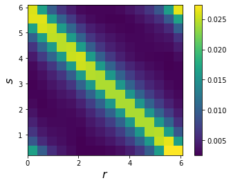
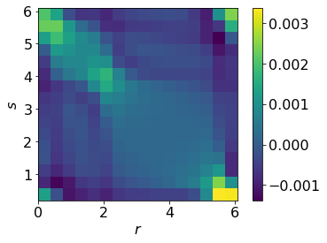
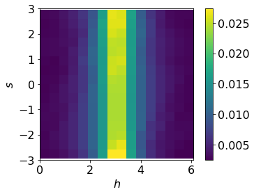
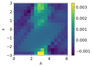
Convolution in the angular direction.

Figure 2d presents an example of the measurement data $\lambda(x_{r},x_{s})$ and $\lambda(x_{r},x_{s})-\lambda_{0}(x_{r},x_{s})$. Notice that the main signal concentrates upon the diagonal part and the left-lower and right-upper corners. Due to the circular tomography geometry, it is convenient to “shear” the measurement data by introducing a new angular variable $h=r-s$, where the difference here is understood modulus $2\pi$. As we shall see, this shearing step significantly simplifies the architecture of the NNs. Under the new parameterization, the measurement data is

$$d(h,s)\equiv d(x_{h+s},x_{s})=d((\cos(s+h),\sin(s+h)),(\cos(s),\sin(s))).$$ (3.1)

By also writing $\mu(\rho,\theta)\equiv\mu((\rho\cos(\theta),\rho\sin(\theta)))$ in the polar coordinates, the linear dependence of $d(h,s)$ on $\tilde{\mu}$ in (2.18) and (2.19) states that there exists a kernel distribution $K(h,s,\rho,\theta)$ such that

$$d(h,s)=\int_{0}^{1}\int_{0}^{2\pi}K(h,s,\rho,\theta)\tilde{\mu}(\rho,\theta)\,\mathrm{d}\rho\,\mathrm{d}\theta.$$ (3.2)

The following proposition states that this can in fact be written as a convolution in the angular direction.

Proposition 1.

There exists a function $\kappa(h,\rho,\cdot)$ periodic in the last argument such that

$$K(h,s,\rho,\theta)=\kappa(h,\rho,s-\theta).$$ (3.3)

The proof of this proposition uses some basic formulas summarized in the following lemma.

Lemma 2.

If $R\in\mathbb{R}^{2\times 2}$ is a rotation matrix, then

$$\beta[\mu_{0}](Rx,Ry) =\beta[\mu_{0}](x,y),$$ (3.4)

$$G_{0}(x,v,x^{\prime},v^{\prime}) =G_{0}(Rx,Rv,Rx^{\prime},Rv^{\prime}).$$ (3.5)

Proof.

The definition of $\beta$ indicates $\beta[\mu_{0}](x,y)=\mu_{0}|x-y|$. Thus 3.4 holds.

Denote the distribution kernel of $\mathcal{L}_{0}\mathcal{S}_{0}$ by $L_{0}(x,v,x^{\prime},v^{\prime})$. Since $\mathcal{G}_{0}=(\mathcal{I}-\mathcal{L}_{0}\mathcal{S}_{0})^{-1}$, we just need to check $L_{0}(Rx,Rv,Rx^{\prime},Rv^{\prime})=L_{0}(x,v,x^{\prime},v^{\prime})$. Notice that the operator $\mathcal{L}\mathcal{S}$ is defined as

$$\mathcal{L}\mathcal{S}Q(x,v) =\int_{0}^{t}\exp\left(-\beta[\mu_{t}](x,x-\tau v)\right)\mu(x-\tau v)\int_{\mathbb{S}^{1}}\sigma(v\cdot v^{\prime})Q(x-\tau v,v^{\prime})\,\mathrm{d}v^{\prime}\,\mathrm{d}\tau$$ (3.6)

$$=\int_{\Omega}\int_{\mathbb{S}^{1}}\frac{\delta(v-\widehat{x-x^{\prime}})}{|x-x^{\prime}|}\exp\left(-\beta[\mu_{t}](x,x^{\prime})\right)\mu(x^{\prime})\sigma(v\cdot v^{\prime})Q(x^{\prime},v^{\prime})\,\mathrm{d}x^{\prime}\,\mathrm{d}v^{\prime}.$$

Then the kernel $L_{0}$ reads

$$L_{0}(x,v,x^{\prime},v^{\prime})=\frac{\delta(v-\widehat{x-x^{\prime}})}{|x-x^{\prime}|}\exp\left(-\beta[\mu_{t,0}](x,x^{\prime})\right)\mu_{0}\sigma(v\cdot v^{\prime}).$$

Since $\delta(Rv-R(\widehat{x-x^{\prime}}))=\delta(v-\widehat{x-x^{\prime}})$, $Rv\cdot Rv^{\prime}=v\cdot v^{\prime}$ and 3.4, one can directly obtain

$$L_{0}(Rx,Rv,Rx^{\prime},Rv^{\prime})=L_{0}(x,v,x^{\prime},v^{\prime}).$$

This completes the proof. ∎

Proof of Proposition 1.

To prove 3.3, one needs to show that, for any $\rho\in[0,1)$ and any $h\in[-\pi,\pi)$ and $s,\psi\in[0,2\pi)$,

$$d(h,s+\psi)=\int_{0}^{1}\int_{0}^{2\pi}K(h,s,\rho,\theta)\tilde{\mu}(\rho,\theta+\psi)\,\mathrm{d}\rho\,\mathrm{d}\theta$$ (3.7)

holds. Notice 2.20 that $d$ has two parts. We study them one by one. Define the rotation matrix $R=\begin{pmatrix}\cos(\psi)&-\sin(\psi)\\ \sin(\psi)&\cos(\psi)\end{pmatrix}$, then

$$d_{1}(h,s+\psi)=d_{1}(Rx_{r},Rx_{s}) =-\int_{\nu(Rx_{r})\cdot v>0}\nu(Rx_{r})\cdot v\int_{\Omega}G_{0}\left(Rx_{r},v,x,\widehat{x-Rx_{s}}\right)$$

$$\qquad\times\exp\left(-\beta[\mu_{t,0}](Rx_{s},x)\right)\beta[\tilde{\mu}](Rx_{s},x)h(\nu(Rx_{s})\cdot\widehat{x-Rx_{s}})\,\mathrm{d}v\,\mathrm{d}x.$$

Since $\Omega$ is a disk, the integral keeps unchanged if we change of variables as $v\to Rv$ and $x\to Rx$. Using $\nu(Rx_{r})\cdot Rv=\nu(x_{r})\cdot v$, 3.5 and 3.4 to eliminate the rotation and changing the variable again as $Rv\to v$ and $Rx\to x$, we obtain

$$d_{1}(h,s+\psi)=d_{1}(Rx_{r},Rx_{s}) =-\int_{\nu(x_{r})\cdot v>0}\nu(x_{r})\cdot v\int_{\Omega}G_{0}\left(x_{r},v,x,\widehat{x-x_{s}}\right)$$

$$\qquad\times\exp\left(-\beta[\mu_{t,0}](x_{s},x)\right)\beta[\tilde{\mu}](Rx_{s},Rx)h(\nu(x_{s})\cdot\widehat{x-x_{s}})\,\mathrm{d}v\,\mathrm{d}x.$$

This completes the proof of the $d_{1}$ part.

Next we study the second part $d_{2}$. Noticing 3.6, we obtain the kernel distribution $E_{1}(x,v,x^{\prime},v^{\prime})$

$$E(x,v,x^{\prime},v^{\prime})=\frac{\delta(v-\widehat{x-x^{\prime}})}{|x-x^{\prime}|}\exp\left(-\beta[\mu_{t,0}](x,x^{\prime})\right)\sigma(v\cdot v^{\prime})\left(-\beta[\tilde{\mu}](x,x^{\prime})+\tilde{\mu}(x^{\prime})\right).$$

Using 3.4, we have

$$E_{1}(Rx,Rv,Rx^{\prime},Rv^{\prime})=\frac{\delta(v-\widehat{x-x^{\prime}})}{|x-x^{\prime}|}\exp\left(-\beta[\mu_{t,0}](x,x^{\prime})\right)\sigma(v\cdot v^{\prime})\left(-\beta[\tilde{\mu}](Rx,Rx^{\prime})+\tilde{\mu}(Rx^{\prime})\right).$$

Then using the same technique in the proof of the first part, we can show that 3.7 also holds for the second part. This completes the proof. ∎

Proposition 1 shows that $K$ acts on $\tilde{\mu}$ in the angular direction by a convolution, i.e.,

$$d(h,s)=\int_{0}^{1}(\kappa(h,\rho,\cdot)*\tilde{\mu}(\rho,\cdot))(s)\,\mathrm{d}\rho.$$ (3.8)

This effectively reduces the forward map to a family of 1D convolutions, parameterized by $\rho$ and $h$.

Till now all the analysis is in the continuous space. One can apply a discretization on the RTE 1.1 by the finite volume method on the space and discrete velocity method on the direction domain [30]. The kernel distribution $G_{0}$ and $E$ are replaced by its discrete version. The actual discretization is often problem-dependent and we leave it to Section 4. Here with a slight abuse of notation, we use the same letters to denote the continuous kernels, variables and their discretization. Then the discretization version of 3.8 is

$$d(h,s)\approx\sum_{\rho}(\kappa(h,\rho,\cdot)*\tilde{\mu}(\rho,\cdot))(s).$$ (3.9)

Neural network architecture.

The perturbative analysis shows that if $\tilde{\mu}$ is sufficiently small, the forward map $\tilde{\mu}(\rho,\theta)\to\tilde{\lambda}(h,s)$ can be approximated by 3.9. This indicates that the forward map 3.9 can be approximated by a convolution layer for small $\tilde{\mu}$. For larger $\tilde{\mu}$, this linear approximation is no longer accurate. In order to extend the neural network for 3.9 to the nonlinear case, we propose to increase the number of convolution layers and include nonlinear activation functions, as shown in Algorithm 1. Here ${{\sf{Conv1d}}}[\alpha,w,{{\sf{ReLU}}}]$ stands for a one-dimensional layer with channel number $\alpha$, window size $w$, and activation function as ${{\sf{ReLU}}}$. Note that because the value of the measurement data ranges in $\mathbb{R}$, no activation function is applied after the last layer. Since the convolution in 3.9 is global, the architectural parameters are chosen with

$$wN_{\mathrm{cnn}}\geq N_{s}$$ (3.10)

so that the resulting network is capable of capturing global interactions. When $N_{s}$ is large, it is possible that the recently proposed multiscale neural networks, for example MNN-$\mathcal{H}$-net [25], MNN-$\mathcal{H}^{2}$-net [24], and BCR-net [23], are more efficient for such global interactions. However in order to simplify the presentation, the discussion here sticks to the convolutional layers.

1:$\alpha$, $w$, $N_{\mathrm{cnn}}\in\mathbb{N}^{+}$, $\tilde{\mu}\in\mathbb{R}^{N_{\rho}\times N_{\theta}}$

2:$\tilde{\lambda}\in\mathbb{R}^{N_{h}\times N_{s}}$

3:$\xi^{(0)}=\tilde{\mu}$ with $\rho$ as the channel direction

4:for $k$ from $1$ to $N_{\mathrm{cnn}}-1$ by $1$ do

5:    $\xi^{(k)}\leftarrow{{\sf{Conv1d}}}[\alpha,w,{{\sf{ReLU}}}](\xi^{(k-1)})$

6:end for

7:$\tilde{\lambda}\leftarrow{{\sf{Conv1d}}}[N_{h},w,{{\sf{id}}}](\xi^{(N_{\mathrm{cnn}}-1)})$

8:return $\tilde{\lambda}$

Algorithm 1 Neural network architecture for the forward problem $\tilde{\mu}\to\tilde{\lambda}$.

3.2 Inverse problem of OT

The perturbative analysis shows that if $\tilde{\mu}$ is sufficiently small, the forward map can be approximated by

$$\tilde{\lambda}\approx K\tilde{\mu},$$ (3.11)

which is the operator notation of the discretization 3.9. Here $\tilde{\mu}$ is a vector indexed by $(\rho,\theta)$, $\tilde{\lambda}$ is a vector indexed by $(h,s)$, and $K$ is a matrix with row indexed by $(h,s)$ and column indexed by $(\rho,\theta)$. The filtered back-projection method [29] suggests the following formula to recover $\tilde{\mu}$:

$$\tilde{\mu}\approx(K^{\mathsf{T}}K+\epsilon I)^{-1}K^{\mathsf{T}}\tilde{\lambda}.$$ (3.12)

Since $K^{\mathsf{T}}\tilde{\lambda}$ can also be written as a family of convolutions

$$(K^{\mathsf{T}}\tilde{\lambda})(\rho,\theta)=\sum_{h}(\kappa(h,\rho,\cdot)*\tilde{\lambda}(h,\cdot))(\theta),$$ (3.13)

the application of $K^{\mathsf{T}}$ to $\tilde{\lambda}$ can be approximated with a one-dimensional convolutional neural network, similar to $K$. For the part $K^{\mathsf{T}}K+\epsilon I$, which can be viewed as a post-processing in the $(\rho,\theta)$ space, we implement this with several two-dimensional convolutional layers for simplicity. However, for problems with larger sizes, multiscale neural networks such as [25, 24, 23] can be also used. The resulting architecture for the inverse map is summarized in Algorithm 2 and illustrated in Fig. 3

1:$\alpha_{1},\alpha_{2}$, $w_{1},w_{2}$, $N_{\mathrm{cnn}_{1}}$, $N_{\mathrm{cnn}_{2}}\in\mathbb{N}^{+}$, $\tilde{\lambda}\in\mathbb{R}^{N_{h}\times N_{s}}$

2:$\tilde{\mu}\in\mathbb{R}^{N_{\rho}\times N_{\theta}}$

3:$\zeta^{(0)}=\tilde{\lambda}$ with $h$ as the channel direction

4:for $k$ from $1$ to $N_{\mathrm{cnn}_{1}}$ by $1$ do

5:    $\zeta^{(k)}\leftarrow{{\sf{Conv1d}}}[\alpha_{1},w_{1},{{\sf{ReLU}}}](\zeta^{(k-1)})$

6:end for

7:$\xi^{(0)}\leftarrow\zeta^{(N_{\mathrm{cnn}_{1}})}$

8:for $k$ from $1$ to $N_{\mathrm{cnn}_{2}}-1$ by $1$ do

9:    $\xi^{(k)}\leftarrow{{\sf{Conv2d}}}[\alpha_{2},w_{2},{{\sf{ReLU}}}](\xi^{(k-1)})$

10:end for

11:$\tilde{\mu}\leftarrow{{\sf{Conv2d}}}[1,w_{2},{{\sf{id}}}](\xi^{(N_{\mathrm{cnn}_{2}}-1)})$

12:return $\tilde{\mu}$

Algorithm 2 Neural network architecture for the inverse problem $\tilde{\lambda}\to\tilde{\mu}$.

Figure 3: Neural network architecture for the inverse map of OT.

4 Numerical tests

This section reports the numerical performance of the proposed neural network architectures for the forward and inverse maps.

4.1 Experimental setup

The RTE in 1.1 is discretized with a finite volume method in $x$ and a discrete velocity method in $v$. The upwind scheme is used for the convection term and the composite trapezoidal rule is applied for the integral of the scattering term. The value of $\sigma(v^{\prime}\cdot v)$ is replaced by its value on the discretization points with a scaling such that its numerical quadrature is $1$. The multi-level method proposed in [30] is adopted to solve the discrete system. The domain $\Omega$ is partitioned by triangle mesh with $6976$ elements and $3553$ points. The direction $v$ is uniformly discretized using $32$ points. In the polar coordinates, the domain $(\rho,\theta)\in[0,1]\times[0,2\pi)$ is partitioned by a uniformly Cartesian mesh with $96\times 192$ points. As a technical note, since Algorithms 1 and 2 are designed for the scattering coefficient in the polar coordinates, the scattering coefficient on the triangle mesh is treated as a piece-constant function and it is further interpolated on to the polar grid.

To mimic the setup of realistic medical applications, $\Omega$ is a disc with the radius equal to $20\mathrm{mm}$ and the background scattering and absorption coefficient are $1\mathrm{mm}^{-1}$ and $0.01\mathrm{mm}^{-1}$, respectively [31, 9, 62]. The parameter $g$ in 1.2 is set as $g=0.9$, a typical value of biological tissues. In the experiment, $N_{s}=16$ light sources and $N_{r}=16$ receivers are equidistantly placed on the boundary of the domain with a half spacing shift (see Fig. 1). The source light is an angular independent pointolite, i.e., the $s$-th light source is $F(x,v)=\delta(x-x_{s})$.

The NN is implemented with Keras [14] running on top of TensorFlow [1]. Nadam is chosen as the optimizer [19] and the mean squared error is used as the loss function. The parameters of the network are initialized by Xavier initialization [32]. In the training process, the batch size and the learning rate is firstly set as $16$ and $10^{-3}$ respectively, and the NN is trained $100$ epochs. Then we increase the batch size by a factor $2$ till to $256$ with the learning rate unchanged, and then decrease the learning rate by a factor $10^{1/2}$ to $10^{-5}$ with the batch size fixed as $256$. In each step, we train the NN $50$ epochs. The selection of the channel number $\alpha$, number of convolution layers $N_{\mathrm{cnn}}$ and the window size $w$ will be discussed in the numerical results.

4.2 Numerical results

For a fixed scattering coefficient field $\mu$, $\lambda(h,s)=\lambda((\cos(s+h),\sin(s+h)),(\cos(s),\sin(s)))$ stands for the exact measurement data solved by numerical discretization of 1.1. The prediction of the forward NN from $\mu$ is denoted by $\lambda^{\mathrm{NN}}$, while the one of the inverse NN from $\lambda$ is denoted by $\mu^{\mathrm{NN}}$. The accuracy for the forward problem is measured by the relative error in the $\ell^{2}$ norm:

$$\frac{\|\lambda-\lambda^{\mathrm{NN}}\|_{\ell^{2}}}{\|\lambda\|_{\ell^{2}}}.$$ (4.1)

For each experiment, the test error is then obtained by averaging 4.1 over a given set of test samples. The numerical results presented below are obtained by repeating the training process three times, using different random seeds for the NN initialization.

The scattering coefficient $\mu(x)$ is assumed to be piecewise constant. For each sample $\mu(x)$, we randomly generate $N_{e}$ ellipses in $\Omega$ and set $\mu(x)=2\mathrm{mm}^{-1}$ in the ellipses and $1\mathrm{mm}^{-1}$ otherwise. For each ellipse, the width and height are sampled from the uniform distributions $\mathcal{U}(0.0075,0.015)$ and $\mathcal{U}(0.00375,0.0075)$, respectively, the direction is uniformly random over the unit circle, and the position is uniformly sampled in the disk. It is also required that each ellipse lies in the disk and there is no intersection between each two ellipses. For each test, $10,204$ samples $\{(\mu_{i},\lambda_{i})\}$ are generated with $8192$ used for training and the remaining 2048 for testing.

While Algorithms 1 and 2 assume for simplicity that $N_{\theta}=N_{s}$, this is often not the case in the experimental setup. To deal with this issue, for the forward problem we first compress $\mu$ from $N_{r}\times N_{\theta}$ to $\alpha\times N_{s}$ by a one-dimensional convolution layer with channel number $\alpha$, window size $N_{r}/N_{s}$, and strides $N_{r}/N_{s}$. For the inverse problem, an interpolation operator for extending the data of size $\alpha\times N_{s}$ to $N_{r}\times N_{\theta}$ is added after the one-dimensional convolution neural networks. In the implementation, the interpolation is implemented by two layers. The first layer interpolates the data of size $\alpha\times N_{s}$ along with the angular direction to $\alpha\times N_{\theta}$ by a one-dimensional convolution layer with channel number $\alpha\times N_{\theta}/N_{s}$ and window size $1$, and a column major reshape. The second layer interpolates the data of size $\alpha\times N_{\theta}$ along with the radial direction to $N_{r}\times N_{\theta}$ by a convolution layer with channel number $N_{r}$ and window size $1$.

Forward problem.

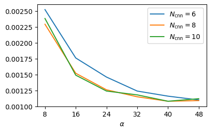
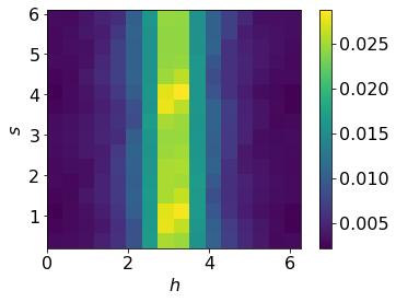
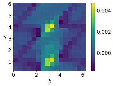
The data set is generated with the number of ellipses $N_{e}=4$ and the window size $w$ in Algorithm 1 is set to be $5$. Multiple numerical experiments are performed to study how the test error depends on the channel number $\alpha$ and the convolution layer number $N_{\mathrm{cnn}}$, with the results presented in Fig. 4. As the number of channels increases, the test error first consistently decreases and then saturates. The same is observed for the number of convolution layers. The choices of the hyper-parameters $\alpha=32$ and $N_{\mathrm{cnn}}=8$ offers a reasonable balance between accuracy and efficiency. For this specific case, the number of parameters is $7.5\times 10^{4}$ and the test error is $1.1\times 10^{-3}$. Figure 5d illustrates the NN prediction $\lambda^{\mathrm{NN}}$ and its corresponding references $\lambda$ of a sample in the test data.

Figure 4: The test error for different channel numbers $\alpha$ and different convolution layer numbers $N_{\mathrm{cnn}}$.

(a) $\lambda(h,s)$

(b) $\lambda^{\mathrm{NN}}(h,s)$

(c) $\lambda(h,s)-\lambda_{0}(h,s)$

(d) $\lambda^{\mathrm{NN}}(h,s)-\lambda_{0}(h,s)$

Figure 5: Illustration of a sample in the test data for the forward problem with the number of ellipses $N_{e}=4$ in $\Omega$. The channel number $\alpha=32$ and the convolution layer number $N_{\mathrm{cnn}}=8$.

Inverse problem.

Two date sets corresponding to $N_{e}=2,4$ are generated. The hyper-parameters in Algorithm 2 are set as $(\alpha_{1}=32,w_{1}=5,N_{\mathrm{cnn}_{1}}=6)$ and $(\alpha_{2}=4,w_{2}=3\times 3,N_{\mathrm{cnn}_{2}}=5)$ and the number of parameters in NN is $4.8\times 10^{4}$. To model the uncertainty in the measurement data, we introduce noises to the albedo operator in the data set by defining $\lambda_{i}^{\delta}\equiv(1+Z_{i}\delta)\lambda_{i}$, where $Z_{i}$ is a Gaussian random variable with zero mean and unity variation and $\delta$ controls the signal-to-noise ratio. For each noisy level $\delta=0$, $0.5\%$, $1\%$, $2\%$ and $5\%$, an independent NN is trained and tested with the noisy data set $\{(\lambda_{i}^{\delta},\mu_{i})\}$. Note that in our experiments the mean of $\frac{\|\lambda-\lambda_{0}\|}{\lambda}$ for all the samples is about $5\%$ and hence the signal-to-noise ratio for the difference $\lambda-\lambda_{0}$ is almost $100\%$ when the noise level $\delta=5\%$.

(a) Reference $\mu$

(b) $\mu^{\mathrm{NN}}$ with $\delta=0$

(c) $\mu^{\mathrm{NN}}$ with $\delta=0.5\%$

(d) $\mu^{\mathrm{NN}}$ with $\delta=1\%$

(e) $\mu^{\mathrm{NN}}$ with $\delta=2\%$

(f) $\mu^{\mathrm{NN}}$ with $\delta=5\%$

Figure 6: NN prediction of a sample in the test data for the number of ellipses $N_{e}=2$ in $\Omega$ and for different noise level $\delta=0,0.5\%,1\%,2\%,5\%$.

(a) Reference $\mu$

(b) $\mu^{\mathrm{NN}}$ with $\delta=0$

(c) $\mu^{\mathrm{NN}}$ with $\delta=0.5\%$

(d) $\mu^{\mathrm{NN}}$ with $\delta=1\%$

(e) $\mu^{\mathrm{NN}}$ with $\delta=2\%$

(f) $\mu^{\mathrm{NN}}$ with $\delta=5\%$

Figure 7: NN prediction of a sample in the test data for the number of ellipses $N_{e}=4$ in $\Omega$ and for different noise level $\delta=0,0.5\%,1\%,2\%,5\%$.

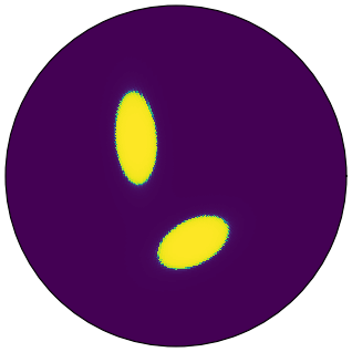
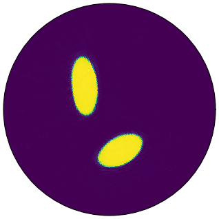
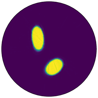
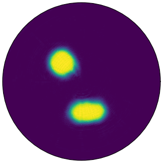
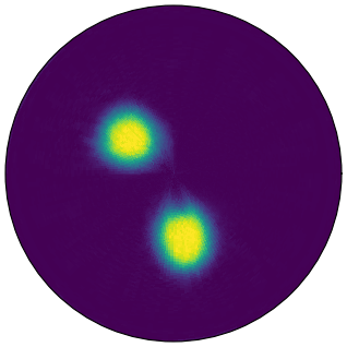
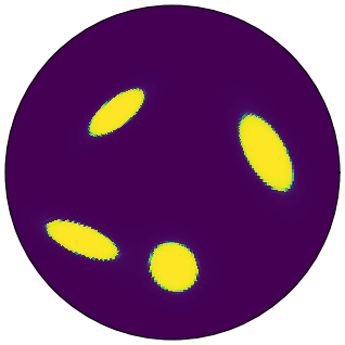
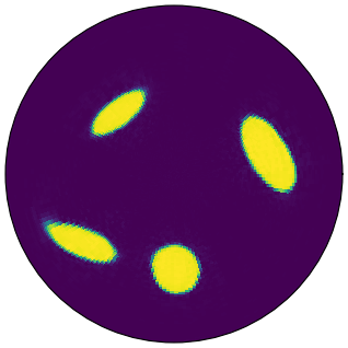
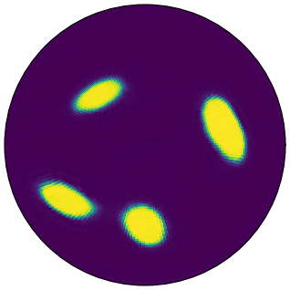
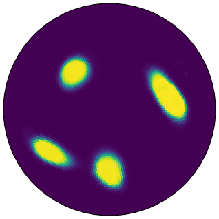
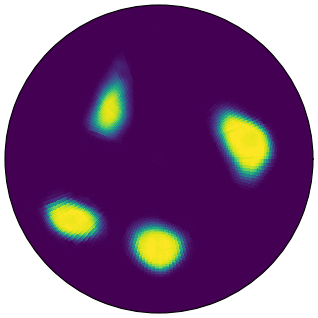
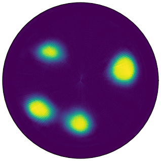
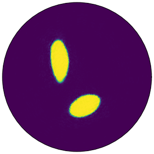
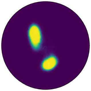
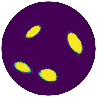
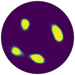
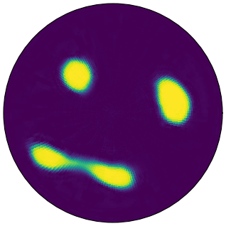
Figures 6 and 7 show samples in the test data for different noise level $\delta$ and different number of ellipses $N_{e}$ in $\Omega$. When there is no noise in the measurement data, the NN offers an accurate prediction of the scattering coefficient $\mu$, in the position, shape and direction of the ellipses. For the small noise levels, for example $\delta=0.5\%$ and $1\%$, the boundary of the shapes in the prediction is blurred while the position and direction of the ellipses are still correct. As the noise level $\delta$ increases, the shapes become fuzzy but the position and number of shapes are still correctly predicted. This demonstrates the NN architecture in Algorithm 2 is capable of learning the inverse problem of OT.

To test the generalization performance of the NN, we train the NN using the data set of $N_{e}=2$ at a given noise level and test the NN by the data of $N_{e}=4$ with the same noise level (and vice versa). The results, summarized in Fig. 8, indicate that the NN trained by the data, with two inclusions is capable of recovering the measurement data of the case with four inclusions, and vice versa. This is an indication that the trained NN is capable of predicting beyond the training scenario.

(a) Reference $\mu$ for $N_{e}=2$

(b) $\mu^{\mathrm{NN}}$ with $\delta=0$

(c) $\mu^{\mathrm{NN}}$ with $\delta=0.5\%$

(d) $\mu^{\mathrm{NN}}$ with $\delta=1\%$

(e) Reference $\mu$ for $N_{e}=4$

(f) $\mu^{\mathrm{NN}}$ with $\delta=0\%$

(g) $\mu^{\mathrm{NN}}$ with $\delta=0.5\%$

(h) $\mu^{\mathrm{NN}}$ with $\delta=1\%$

Figure 8: NN generation test. The upper figures: the NN is trained by the data of the number of ellipses $N_{e}=4$ in $\Omega$ with noise level $\delta=0$ $0.5\%$ or $1\%$ and test by the data of $N_{e}=2$ with the same noise level. The lower figures correspond the case of training data $N_{e}=2$ and test data $N_{e}=4$.

5 Discussions

This paper presents a neural network approach for OT problems. Mathematically, these NNs approximate the forward and inverse maps between the scattering coefficient and the kernel distribution of the albedo operator. The perturbative analysis, which indicates that the linearized forward map can be represented by a one-dimensional convolution with multiple channels, inspires the design of the NN architectures.

NNs have offered a few clear advantages in approximating the forward and inverse problems. For both the forward and inverse maps, once the NN is trained, applying the map is significantly accelerated as it only involves a single inference with the trained NN. For the inverse problem, two critical issues for more traditional approaches are the choices of the solution algorithm and the regularization term. NNs seem to bypass the algorithm issue by choosing an appropriate architecture and learning the map from the data, and at the same time, identify an appropriate regularization by automatically learning the key features from the training set. Numerical results also demonstrate that the proposed NNs are capable of approximating the forward and inverse maps accurately. However, although empirically encouraging, theoretical justification of these advantages require significant work.

The discussion in this paper focuses on the reconstruction of the scattering coefficient. Using a similar analysis, one can extend the work to the reconstruction of the absorption coefficient or both. The analysis in this paper can also extended to the three-dimensional OT problems by leveraging recent work such as [16].

References

- [1] M. Abadi et al. Tensorflow: A system for large-scale machine learning. In OSDI, volume 16, pages 265–283, 2016.
- [2] J. Adler and O. Öktem. Solving ill-posed inverse problems using iterative deep neural networks. Inverse Problems, 33(12):124007, 2017.
- [3] M. Araya-Polo, J. Jennings, A. Adler, and T. Dahlke. Deep-learning tomography. The Leading Edge, 37(1):58–66, 2018.
- [4] S. R. Arridge and J. C. Schotland. Optical tomography: forward and inverse problems. Inverse problems, 25(12):123010, 2009.
- [5] G. Bal. Introduction to inverse problems. Lecture Notes-Department of Statistics and Mathematics, University of Chicago, 2019.
- [6] G. Bal and A. Jollivet. Stability estimates in stationary inverse transport. Inverse Problems and Imaging, 2(4):427–454, 2008.
- [7] L. Bar and N. Sochen. Unsupervised deep learning algorithm for PDE-based forward and inverse problems. arXiv preprint arXiv:1904.05417, 2019.
- [8] J. Berg and K. Nyström. A unified deep artificial neural network approach to partial differential equations in complex geometries. Neurocomputing, 317:28–41, 2018.
- [9] B. Bi, B. Han, W. Han, J. Tang, and L. Li. Image reconstruction for diffuse optical tomography based on radiative transfer equation. Computational and mathematical methods in medicine, 2015, 2015.
- [10] D. A. Boas, A. M. Dale, and M. A. Franceschini. Diffuse optical imaging of brain activation: approaches to optimizing image sensitivity, resolution, and accuracy. Neuroimage, 23:S275–S288, 2004.
- [11] G. Carleo and M. Troyer. Solving the quantum many-body problem with artificial neural networks. Science, 355(6325):602–606, 2017.
- [12] K. Case and P. Zweifel. Existence and uniqueness theorems for the neutron transport equation. Journal of Mathematical Physics, 4(11):1376–1385, 1963.
- [13] T. F. Chan, G. H. Golub, and P. Mulet. A nonlinear primal-dual method for total variation-based image restoration. SIAM journal on scientific computing, 20(6):1964–1977, 1999.
- [14] F. Chollet et al. Keras. https://keras.io, 2015.
- [15] M. Choulli and P. Stefanov. Reconstruction of the coefficients of the stationary transport equation from boundary measurements. Inverse Problems, 12(5):L19, 1996.
- [16] T. S. Cohen, M. Geiger, J. Köhler, and M. Welling. Spherical CNNs. In International Conference on Learning Representations, 2018.
- [17] G. Cybenko. Approximation by superpositions of a sigmoidal function. Mathematics of control, signals and systems, 2(4):303–314, 1989.
- [18] R. Dautray and J.-L. Lions. Mathematical Analysis and Numerical Methods for Science and Technology: Volume 6 Evolution Problems II. Springer-Verlag Berlin Heidelberg, 2000.
- [19] T. Dozat. Incorporating Nesterov momentum into adam. International Conference on Learning Representations, 2016.
- [20] W. E and B. Yu. The deep Ritz method: A deep learning-based numerical algorithm for solving variational problems. Communications in Mathematics and Statistics, 6(1):1–12, 2018.
- [21] C. Edwards, A. Arbabi, G. Popescu, and L. L. Goddard. Optically monitoring and controlling nanoscale topography during semiconductor etching. Light: Science & Applications, 1(9):e30, 2012.
- [22] H. Egger and M. Schlottbom. An theory for stationary radiative transfer. Applicable Analysis, 93(6):1283–1296, 2014.
- [23] Y. Fan, C. O. Bohorquez, and L. Ying. BCR-Net: a neural network based on the nonstandard wavelet form. Journal of Computational Physics, 384:1–15, 2019.
- [24] Y. Fan, J. Feliu-Fabà, L. Lin, L. Ying, and L. Zepeda-Núñez. A multiscale neural network based on hierarchical nested bases. Research in the Mathematical Sciences, 6(2):21, 2019.
- [25] Y. Fan, L. Lin, L. Ying, and L. Zepeda-Núñez. A multiscale neural network based on hierarchical matrices. arXiv preprint arXiv:1807.01883, 2018.
- [26] Y. Fan and L. Ying. Solving electrical impedance tomography with deep learning. arXiv preprint arXiv:1906.03944, 2019.
- [27] S. Fantini and A. Sassaroli. Near-infrared optical mammography for breast cancer detection with intrinsic contrast. Annals of biomedical engineering, 40(2):398–407, 2012.
- [28] J. Feliu-Faba, Y. Fan, and L. Ying. Meta-learning pseudo-differential operators with deep neural networks. arXiv preprint arXiv:1906.06782, 2019.
- [29] T. Feng, P. Edström, and M. Gulliksson. Levenberg–Marquardt methods for parameter estimation problems in the radiative transfer equation. Inverse Problems, 23(3):879, 2007.
- [30] H. Gao and H. Zhao. A fast-forward solver of radiative transfer equation. Transport Theory and Statistical Physics, 38(3):149–192, 2009.
- [31] H. Gao and H. Zhao. Multilevel bioluminescence tomography based on radiative transfer equation part 1: l1 regularization. Optics Express, 18(3):1854–1871, 2010.
- [32] X. Glorot and Y. Bengio. Understanding the difficulty of training deep feedforward neural networks. In Proceedings of the thirteenth international conference on artificial intelligence and statistics, pages 249–256, 2010.
- [33] I. Goodfellow, Y. Bengio, A. Courville, and Y. Bengio. Deep learning, volume 1. MIT press Cambridge, 2016.
- [34] E. Haber, U. M. Ascher, and D. Oldenburg. On optimization techniques for solving nonlinear inverse problems. Inverse problems, 16(5):1263, 2000.
- [35] J. Han, A. Jentzen, and W. E. Solving high-dimensional partial differential equations using deep learning. Proceedings of the National Academy of Sciences, 115(34):8505–8510, 2018.
- [36] J. Han, L. Zhang, R. Car, and W. E. Deep potential: A general representation of a many-body potential energy surface. Communications in Computational Physics, 23(3):629–639, 2018.
- [37] M. Hanke. Regularizing properties of a truncated Newton-CG algorithm for nonlinear inverse problems. Numerical Functional Analysis and Optimization, 18(9-10):971–993, 1997.
- [38] L. G. Henyey and J. L. Greenstein. Diffuse radiation in the galaxy. The Astrophysical Journal, 93:70–83, 1941.
- [39] G. Hinton, L. Deng, D. Yu, G. E. Dahl, A. r. Mohamed, N. Jaitly, A. Senior, V. Vanhoucke, P. Nguyen, T. N. Sainath, and B. Kingsbury. Deep neural networks for acoustic modeling in speech recognition: The shared views of four research groups. IEEE Signal Processing Magazine, 29(6):82–97, 2012.
- [40] S. R. H. Hoole. Artificial neural networks in the solution of inverse electromagnetic field problems. IEEE transactions on Magnetics, 29(2):1931–1934, 1993.
- [41] H. Kabir, Y. Wang, M. Yu, and Q.-J. Zhang. Neural network inverse modeling and applications to microwave filter design. IEEE Transactions on Microwave Theory and Techniques, 56(4):867–879, 2008.
- [42] J. P. Kaipio, V. Kolehmainen, M. Vauhkonen, and E. Somersalo. Inverse problems with structural prior information. Inverse problems, 15(3):713, 1999.
- [43] Y. Khoo, J. Lu, and L. Ying. Solving parametric PDE problems with artificial neural networks. arXiv preprint arXiv:1707.03351, 2017.
- [44] Y. Khoo, J. Lu, and L. Ying. Solving for high-dimensional committor functions using artificial neural networks. Research in the Mathematical Sciences, 6(1):1, 2019.
- [45] Y. Khoo and L. Ying. SwitchNet: a neural network model for forward and inverse scattering problems. arXiv preprint arXiv:1810.09675, 2018.
- [46] A. Krizhevsky, I. Sutskever, and G. E. Hinton. ImageNet classification with deep convolutional neural networks. In Proceedings of the 25th International Conference on Neural Information Processing Systems - Volume 1, NIPS’12, pages 1097–1105, USA, 2012. Curran Associates Inc.
- [47] G. Kutyniok, P. Petersen, M. Raslan, and R. Schneider. A theoretical analysis of deep neural networks and parametric PDEs. arXiv preprint arXiv:1904.00377, 2019.
- [48] Y. LeCun, Y. Bengio, and G. Hinton. Deep learning. Nature, 521(436), 2015.
- [49] C. Leng, D. Yu, S. Zhang, Y. An, and Y. Hu. Reconstruction method for optical tomography based on the linearized Bregman iteration with sparse regularization. Computational and mathematical methods in medicine, 2015, 2015.
- [50] M. K. K. Leung, H. Y. Xiong, L. J. Lee, and B. J. Frey. Deep learning of the tissue-regulated splicing code. Bioinformatics, 30(12):i121–i129, 2014.
- [51] Y. Li, J. Lu, and A. Mao. Variational training of neural network approximations of solution maps for physical models. arXiv preprint arXiv:1905.02789, 2019.
- [52] Z. Long, Y. Lu, X. Ma, and B. Dong. PDE-net: Learning PDEs from data. In J. Dy and A. Krause, editors, Proceedings of the 35th International Conference on Machine Learning, volume 80 of Proceedings of Machine Learning Research, pages 3208–3216, Stockholmsmässan, Stockholm Sweden, 10–15 Jul 2018. PMLR.
- [53] A. Lucas, M. Iliadis, R. Molina, and A. K. Katsaggelos. Using deep neural networks for inverse problems in imaging: beyond analytical methods. IEEE Signal Processing Magazine, 35(1):20–36, 2018.
- [54] J. Ma, R. P. Sheridan, A. Liaw, G. E. Dahl, and V. Svetnik. Deep neural nets as a method for quantitative structure-activity relationships. Journal of Chemical Information and Modeling, 55(2):263–274, 2015.
- [55] M. Raissi and G. E. Karniadakis. Hidden physics models: Machine learning of nonlinear partial differential equations. Journal of Computational Physics, 357:125 – 141, 2018.
- [56] M. Raissi, P. Perdikaris, and G. E. Karniadakis. Physics-informed neural networks: A deep learning framework for solving forward and inverse problems involving nonlinear partial differential equations. Journal of Computational Physics, 378:686–707, 2019.
- [57] K. Rudd and S. Ferrari. A constrained integration (CINT) approach to solving partial differential equations using artificial neural networks. Neurocomputing, 155:277–285, 2015.
- [58] J. Schmidhuber. Deep learning in neural networks: An overview. Neural Networks, 61:85–117, 2015.
- [59] P. Stefanov et al. Optical tomography in two dimensions. Methods and Applications of Analysis, 10(1):001–010, 2003.
- [60] I. Sutskever, O. Vinyals, and Q. V. Le. Sequence to sequence learning with neural networks. In Z. Ghahramani, M. Welling, C. Cortes, N. D. Lawrence, and K. Q. Weinberger, editors, Advances in Neural Information Processing Systems 27, pages 3104–3112. Curran Associates, Inc., 2014.
- [61] C. Tan, S. Lv, F. Dong, and M. Takei. Image reconstruction based on convolutional neural network for electrical resistance tomography. IEEE Sensors Journal, 19(1):196–204, 2018.
- [62] S. Tong, B. Han, Y. Chen, J. Tang, B. Bi, and R. Gu. RTE-based parameter reconstruction with TV + L1 regularization. Journal of Computational and Applied Mathematics, 337:256–273, 2018.
- [63] C. Weitkamp. Lidar: range-resolved optical remote sensing of the atmosphere, volume 102. Springer Science & Business, 2006.
- [64] H. Zhao and Y. Zhong. Instability of an inverse problem for the stationary radiative transport near the diffusion limit. arXiv preprint arXiv:1809.01790, 2018.