Learning Only from Relevant Keywords and Unlabeled Documents

Abstract

We consider a document classification problem where document labels are absent but only relevant keywords of a target class and unlabeled documents are given. Although heuristic methods based on pseudo-labeling have been considered, theoretical understanding of this problem has still been limited. Moreover, previous methods cannot easily incorporate well-developed techniques in supervised text classification. In this paper, we propose a theoretically guaranteed learning framework that is simple to implement and has flexible choices of models, e.g., linear models or neural networks. We demonstrate how to optimize the area under the receiver operating characteristic curve (AUC) effectively and also discuss how to adjust it to optimize other well-known evaluation metrics such as the accuracy and $\mathrm{F}_{1}$-measure. Finally, we show the effectiveness of our framework using benchmark datasets.

1 Introduction

Supervised text classification is a traditional problem in natural language processing that has been studied extensively (Nigam et al., 2000; Sebastiani, 2002; Forman, 2003; Joulin et al., 2016). In this problem, we are given a set of labeled text documents and the goal is to construct a classifier that can classify an unseen document effectively. There are many useful applications for text classification, e.g., sentiment classification (Liu and Zhang, 2012; Medhat et al., 2014), biomedical text mining (Cohen and Hersh, 2005; Huang and Lu, 2015), and social media monitoring (Zeng et al., 2010; Hu and Liu, 2012).

In the real-world, it is impractical to expect that labeled data can always be obtained abundantly. For example, given big data of unlabeled texts, it can be very time-consuming and costly for the labeling task so that we can apply a supervised text classification method. Another example is when the label information is protected due to privacy concerns. These bottlenecks motivate researches on weakly-supervised learning (Zhou, 2017), which focuses on devising a machine learning method that can learn effectively although a lot of labeled data are not accessible.

An alternative is to provide keywords as a hint for classifying a document to a target class. Intuitively, this approach can be much cheaper when the number of documents is huge since the number of keywords does not necessarily grow linearly with the number of documents. Dataless classification is a text classification problem where we are given keywords for each class and unlabeled documents (Chang et al., 2008; Song and Roth, 2014; Chen et al., 2015; Li and Yang, 2018). Note that we do not have access to any labeled documents.

In this paper, we investigate dataless classification in the situation where only the keywords of the target class are given. We regard documents of a class that we have relevant keywords as positive and others as negative. Unlike dataless classification, we have access to only the keywords of the positive class. This problem setting can be considered more difficult than the traditional one since one can always reduce dataless classification to this problem by ignoring negative keywords. This scenario is also highly relevant when the information about negative classes cannot be explicitly described, e.g., in the information retrieval task, we may only have information about the target class of interest.

This problem setting has already been considered by Jin et al. (2017), where they called it lightly-supervised one-class classification. To the best of our knowledge, existing work in dataless classification and lightly-supervised one-class classification neither provide a theoretical guarantee, nor have flexible choices of models and optimization algorithms for this problem.

The goal of this paper is to formalize lightly-supervised one-class classification and develop a reliable and flexible framework to handle this problem effectively. To achieve this goal, we propose a framework that has a theoretical guarantee and allows practitioners to have flexible choices to maximize the performance, e.g., neural network architectures such as convolutional neural networks (Zhang et al., 2015) or recurrent neural networks (Lai et al., 2015). They can also pick an optimization method that is suitable for their model such as Adam (Kingma and Ba, 2014) or AMSGrad (Reddi et al., 2018). These advantages allow us to utilize well-developed supervised-learning text classification methods in our framework.

We point out that the problem of lightly-supervised one-class classification is highly related to binary classification from corrupted labels. Intuitively, the common idea to solve this problem is to use keywords to pseudo-label given documents then performs classification (Jin et al., 2017). However, pseudo-positive and pseudo-negative labels are unreliable since they can be incorrectly labeled. Thus, the learning method should be robust against label corruption. In our framework, we also use relevant keywords to split unlabeled data into two sets. Then, the key idea is to employ a method based on an empirical risk minimization framework (Vapnik, 1998) with a loss function that benefits from a symmetric condition to maximize AUC (Charoenphakdee et al., 2019). We justify the soundness of our method by proving that our proposed framework gives a consistent estimation of the true expected AUC risk as long as the divided two sets have different proportions of positive data. We elucidate this theoretical result by providing an estimation error bound for AUC maximization using a Rademacher complexity measure. Furthermore, we discuss how to adjust our method to optimize other evaluation metrics, which are the accuracy and $\mathrm{F}_{1}$-measure. We also illustrate that label corruption may cause a classifier to pick a wrong decision boundary and suggest to adjust the threshold on the basis of the proportion of positive data in unlabeled data.

2 Preliminaries

In this section, we introduce the notation, review AUC, and an empirical risk minimization framework for optimizing AUC.

2.1 Notation

Let $\boldsymbol{x}\in\mathcal{X}$ be a pattern in the input space $\mathcal{X}$ and $y\in\{-1,1\}$ be a label. We denote $g:\mathcal{X}\to\mathbb{R}$ as a prediction function. Let $\mathbb{E}_{\mathrm{P}}[\cdot]$ and $\mathbb{E}_{\mathrm{N}}[\cdot]$ denote the expectation over the class-conditional probability $p(\boldsymbol{x}|y=1)$ and $p(\boldsymbol{x}|y=-1)$, respectively. Moreover, let $\pi$ denote a class prior $p(y=1)$, i.e., the proportion of positive data.

Loss functions that we will discuss in this paper are in the family of margin losses, where a loss receives one argument $\ell:\mathbb{R}\to\mathbb{R}$. This loss family covers a lot of well-known losses (Bartlett et al., 2006), e.g., the logistic loss, squared loss, and hinge loss. We define the zero-one loss as $\ell_{0\text{-}1}(z)=-\frac{1}{2}\mathrm{sign}(z)+\frac{1}{2},$ where sign$(g(\boldsymbol{x}))=1$ if $g(\boldsymbol{x})>0$, $-1$ if $g(\boldsymbol{x})<0$, and $0$ otherwise. Finally, we consider a symmetric loss as a margin loss $\ell_{\mathrm{sym}}$ that satisfies the symmetric condition $\ell_{\mathrm{sym}}(z)+\ell_{\mathrm{sym}}(-z)=K$, where $K$ is a positive constant. Examples of such losses are the zero-one loss and sigmoid loss (Ghosh et al., 2015). Table 1 provides examples of margin losses in binary classification.

Table 1: Examples of loss functions. A symmetric loss is a loss function such that $\ell(z)+\ell(-z)=K$, where $K$ is a positive constant.

Loss name	$\ell(z)$	Symmetric
Logistic	$\log(1+e^{-z})$	$\times$
Squared	$(1-z)^{2}$	$\times$
Zero-one	$-\frac{1}{2}\mathrm{sign}(z)+\frac{1}{2}$	$\checkmark$
Sigmoid	$\frac{1}{1+\exp(z)}$	$\checkmark$

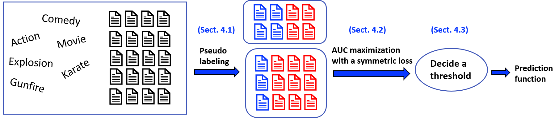
Figure 1: An overview of the framework. Blue documents indicates clean positive data and red documents denote clean negative data in the two sets of data divided by the pseudo-labeling algorithm. Note that labels are not observed by the framework. Sect. denotes a section that describes the procedure for each step.

2.2 Area under the Receiver Operating Characteristic Curve (AUC)

AUC is an evaluation metric for a bipartite ranking task (Cortes and Mohri, 2004; Menon and Williamson, 2016), where we want to find a function that outputs a higher value for positive data than negative data. Moreover, AUC is also a popular metric for a classifier under class imbalance (Menon et al., 2015). It is also known in the literature of statistics as the Wilcoxon-Mann-Whitney statistic (Mann and Whitney, 1947; Hanley and McNeil, 1982).

Let us consider the AUC risk, i.e., bipartite ranking risk (Narasimhan and Agarwal, 2013):

$$R_{\mathrm{AUC}}^{\ell_{0\text{-}1}}(g)=\mathbb{E}_{\mathrm{P}}\left[\mathbb{E}_{\mathrm{N}}\left[\ell_{0\text{-}1}(g(\boldsymbol{x}^{\mathrm{P}}_{i})-g(\boldsymbol{x}^{\mathrm{N}}_{j}))\right]\right]\text{.}$$ (1)

Then, AUC is defined as $\mathrm{AUC}(g)=1-R_{\mathrm{AUC}}^{\ell_{0\text{-}1}}(g)$. It is important to note that unlike many other evaluation metrics, we can evaluate AUC without deciding the threshold for a function $g$. In this paper, we will show that optimizing AUC in our problem setting has a great advantage when no information about the threshold is given since we only have keywords and unlabeled documents.

2.3 Empirical Risk Minimization (ERM) for AUC Maximization

Here, we review a widely used framework in machine learning called the ERM framework  (Vapnik, 1998) for AUC maximization.

The goal of AUC maximization is to minimize the AUC risk in (1) with respect to the zero-one loss $R_{\mathrm{AUC}}^{\ell_{0\text{-}1}}(g)$ (Menon and Williamson, 2016).

Although the goal is to minimize the bipartite ranking risk with respect to the zero-one loss $\ell_{0\text{-}1}$, a surrogate loss $\ell$, e.g., the logistic loss or the squared loss, is instead applied in practice since minimizing $\ell_{0\text{-}1}$ is computationally infeasible (Ben-David et al., 2003; Zhang, 2004; Bartlett et al., 2006; Feldman et al., 2012). Note that we cannot directly minimize the AUC risk in our setting since we do not have access to the positive and negative distributions.

To explain the ERM framework for bipartite ranking, in this section, let us assume that we are given positive data $\{\boldsymbol{x}^{\mathrm{P}}_{i}\}_{i=1}^{n_{\mathrm{P}}}$ and negative data $\{\boldsymbol{x}^{\mathrm{N}}_{j}\}_{j=1}^{n_{\mathrm{N}}}$ drawn from the class-conditional probability densities $p(\boldsymbol{x}|y=1)$ and $p(\boldsymbol{x}|y=-1)$, respectively. Having access to positive and negative data, the ERM framework suggests us to minimize the following empirical risk (Yan et al., 2003; Cortes and Mohri, 2004):

$$\hat{R}_{\mathrm{AUC}}^{\ell}(g)=\frac{1}{n_{\mathrm{P}}n_{\mathrm{N}}}\sum_{i=1}^{n_{\mathrm{P}}}\sum_{j=1}^{n_{\mathrm{N}}}\ell(g(\boldsymbol{x}^{\mathrm{P}}_{i})-g(\boldsymbol{x}^{\mathrm{N}}_{j}))\text{.}$$ (2)

With the given training data and a surrogate loss $\ell$, we can minimize $\hat{R}_{\mathrm{AUC}}^{\ell}(g)$. This risk estimator $\hat{R}_{\mathrm{AUC}}^{\ell}(g)$ is an unbiased and consistent estimator of the true AUC risk (1), which means it converges to the true AUC risk as the number of data increases (Yan et al., 2003; Herschtal and Raskutti, 2004; Gao and Zhou, 2015).

Note that in practice, it is common to apply a regularization method for controlling the bias-variance trade-off of the estimator to avoid overfitting. In this paper, we adopt the ERM framework for minimizing the AUC risk. Note that one challenge of our problem is that we cannot apply the standard AUC risk directly since we have no access to any labeled data.

3 Problem Formulation

In this section, we formulate the problem of learning from keywords and unlabeled data. We are given a set of relevant keywords $W:=\{w_{j}\}_{j=1}^{n_{\mathrm{W}}}$, and unlabeled documents drawn from the following distribution:

$$X_{\mathrm{U}}:=\{\boldsymbol{x}^{\mathrm{U}}_{i}\}_{i=1}^{n_{\mathrm{U}}}\stackrel{{\scriptstyle\mathrm{i.i.d.}}}{{\sim}}p_{\pi}(\boldsymbol{x}),$$

where

$$p_{\pi}(\boldsymbol{x})=\pi p(\boldsymbol{x}|y=1)+(1-\pi)\,p(\boldsymbol{x}|y=-1).$$

The evaluation metric defines the goal of this problem. For example, if we want a ranking function that outputs a large value for positive data, and small otherwise, the well-known evaluation metric is AUC (Agarwal et al., 2005). We will discuss other evaluation metrics, which are the accuracy and $\mathrm{F}_{1}$-measure in Section 4.3.

4 Proposed Framework

In this section, we propose a novel framework for handling this problem systematically. The framework consists of three parts. First, we use relevant keywords to extract pseudo-positive data from the unlabeled data. Then, we employ a symmetric loss function for AUC optimization within the empirical risk minimization framework. Finally, we adjust the threshold of a trained AUC maximizer to further optimize other evaluation metrics. Figure 1 shows an overview of our framework.

4.1 Pseudo-labeling

Here, we propose a simple pseudo-labeling method. We want to emphasize that we do not expect that a pseudo-labeling algorithm is perfect, i.e., pseudo-positive documents may contain negative documents. In Section 4.2, we show that it is possible to maximize AUC effectively even though the labels are highly corrupted.

Since we focus on proposing a general framework that can be used in a wide range of text classification tasks, we use a simple pseudo-labeling method. In practice, one can incorporate prior knowledge such as the specific characteristic of documents to develop a sophisticated and potentially better pseudo-labeling algorithm to further enhance the performance. Our simple pseudo-labeling method is a ranking score based on the document similarities with the cosine similarity between unlabeled documents and keywords. Although we assume some keywords are given, it is hard to guarantee that the given keywords are sufficient to learn effectively. Hence, it is reasonable to sample more similar words to given keywords. In this paper, we used the GloVe model to find similar words Pennington et al. (2014). With a sufficient number of keywords, we calculate the cosine similarity between the set of extended keywords set and each unlabeled document by simply merging all keywords and extended keywords into one document and measure the similarity between this keyword document and each unlabeled document. Finally, we pseudo-label documents to positive if their cosine similarities are in the top-$\phi$%.

Input: Unlabeled documents $\{\boldsymbol{x}^{\mathrm{U}}_{i}\}_{i=1}^{n_{\mathrm{U}}}$, keyword set $W:=\{w_{j}\}_{j=1}^{n_{\mathrm{W}}}$, threshold $\phi\in[0,100]$, weight of original keywords $\alpha\in\mathbb{N}$, sampling factor $\gamma\in\mathbb{N}$.

Output: two sets of pseudo-labeled documents $X_{\mathrm{CP}}$ and $X_{\mathrm{CN}}$

$X_{\mathrm{CP}}:=\{\}$; $X_{\mathrm{CN}}:=\{\}$ foreach $w_{j}$ do

      Add additional ($\alpha$-1) of $w_{j}$ to $W$;

       Find top-$\gamma$ similar words to $w_{j}$ $W_{sim}:=\{w_{j}^{i}\}_{i=1}^{\gamma}$;

       Add $W_{sim}$ to $W$;

end foreach

Compute similarity $s_{i}$ between one document that merges all keywords $W=\{w_{j}\}_{j=1}^{(\alpha+\gamma)n_{\mathrm{W}}}$ and each document $\boldsymbol{x}^{\mathrm{U}}_{i}$;

foreach $\boldsymbol{x}^{\mathrm{U}}_{i}$ do

       if $s_{i}>0$ and in the top-$\phi$(%) then

            Add $\boldsymbol{x}^{\mathrm{U}}_{i}$ to $X_{\mathrm{CP}}$;

       else

            Add $\boldsymbol{x}^{\mathrm{U}}_{i}$ to $X_{\mathrm{CN}}$;

       end if

      

end foreach

return $X_{\mathrm{CP}}$, $X_{\mathrm{CN}}$

Algorithm 1 A pseudo-labeling algorithm

4.2 AUC Optimization from Corrupted Labels

After applying Algorithm 1, we can obtain two sets of data, which we call them a corrupted positive set and a corrupted negative set. Let us define $\theta,\,\theta^{\prime}\in[0,1]$, which indicate the proportion of positive data for the corrupted positive and negative sets, respectively. We assume a mild condition that our pseudo-labeling method can split the data such that the corrupted positive set has a higher proportion of positive data than another set, i.e., $\theta>\theta^{\prime}$. Then, we formulate the data from the two sets as

$$X_{\mathrm{CP}} :=\{\boldsymbol{x}^{\mathrm{CP}}_{i}\}_{i=1}^{n_{\mathrm{CP}}}\stackrel{{\scriptstyle\mathrm{i.i.d.}}}{{\sim}}p_{\theta}(\boldsymbol{x})\text{,}$$

$$X_{\mathrm{CN}} :=\{\boldsymbol{x}^{\mathrm{CN}}_{j}\}_{j=1}^{n_{\mathrm{CN}}}\stackrel{{\scriptstyle\mathrm{i.i.d.}}}{{\sim}}p_{\theta^{\prime}}(\boldsymbol{x})\text{,}$$

where

$$p_{\theta}(\boldsymbol{x}) :=\theta p(\boldsymbol{x}|y=1)+(1-\theta)p(\boldsymbol{x}|y=-1)\text{,}$$

$$p_{\theta^{\prime}}(\boldsymbol{x}) :=\theta^{\prime}p(\boldsymbol{x}|y=1)+(1-\theta^{\prime})p(\boldsymbol{x}|y=-1)\text{.}$$

$X_{\mathrm{CP}}$ and $X_{\mathrm{CN}}$ are the sets of corrupted positive and corrupted negative data, respectively. We utilize the fact that optimizing AUC can be performed effectively even when the data is highly corrupted by using a symmetric loss function (Charoenphakdee et al., 2019). More specifically, let us consider a corrupted AUC risk. First, let us define $\mathbb{E}_{\theta}$ and $\mathbb{E}_{\theta^{\prime}}$ as the expectation over $p_{\theta}$ and $p_{\theta^{\prime}}$, respectively. A corrupted AUC risk is defined as

$$R^{\ell}_{\mathrm{AUC}\text{-}\mathrm{Corr}}(g)=\mathbb{E}_{\theta}[\mathbb{E}_{\theta^{\prime}}[\ell(g(\boldsymbol{x})-g(\boldsymbol{x}^{\prime})))]]\text{.}$$ (3)

Intuitively, the risk (3) is minimized by a function $g$ that gives a higher value on corrupted positive data over corrupted negative data. The following theorem establishes the relationship between the clean AUC risk and corrupted AUC risk.

Theorem 1 (Charoenphakdee et al. (2019)).

Let $\varphi^{\ell}(\boldsymbol{x},\boldsymbol{x}^{\prime})=\ell(g(\boldsymbol{x})-g(\boldsymbol{x}^{\prime}))+\ell(g(\boldsymbol{x}^{\prime})-g(\boldsymbol{x}))$. Then $R^{\ell}_{\mathrm{AUC}\text{-}\mathrm{Corr}}(g)$ can be expressed as

$$\begin{split}&R^{\ell}_{\mathrm{AUC}\text{-}\mathrm{Corr}}(g)=(\theta-\theta^{\prime})R^{\ell}_{\mathrm{AUC}}(g)\\ &+\underbrace{(1-\theta)\theta^{\prime}\mathbb{E}_{\mathrm{P}}[\mathbb{E}_{\mathrm{N}}[\varphi^{\ell}(\boldsymbol{x}^{\mathrm{P}},\boldsymbol{x}^{\mathrm{N}})]]}_{\textup{Excessive term}}\\ &+\underbrace{\frac{\theta\theta^{\prime}}{2}\mathbb{E}_{\mathrm{P^{\prime}}}[\mathbb{E}_{\mathrm{P}}[\varphi^{\ell}(\boldsymbol{x}^{\mathrm{P^{\prime}}},\boldsymbol{x}^{\mathrm{P}})]]}_{\textup{Excessive term}}\\ &+\underbrace{\frac{(1-\theta)(1-\theta^{\prime})}{2}\mathbb{E}_{\mathrm{N^{\prime}}}[\mathbb{E}_{\mathrm{N}}[\varphi^{\ell}(\boldsymbol{x}^{\mathrm{N^{\prime}}},\boldsymbol{x}^{\mathrm{N}})]]}_{\textup{Excessive term}}\text{.}\end{split}$$

Theorem 1 shows that minimizing the corrupted risk $R^{\ell}_{\mathrm{AUC}\text{-}\mathrm{Corr}}(g)$ implies minimizing both the clean risk $R^{\ell}_{\mathrm{AUC}}(g)$ and excessive terms. However, since we only aim to minimize the clean risk, minimizing the corrupted risk may not effectively minimize the clean risk since excessive terms can be minimized instead and lead to overfitting.  Charoenphakdee et al. (2019) showed that with a specific class of losses, excessive terms become constant. The following theorem suggests that by using a family of symmetric losses, the corrupted AUC risk can be expressed as an affine transformation of the clean AUC risk.

Theorem 2 (Charoenphakdee et al. (2019)).

Let $\ell_{\mathrm{sym}}$ be a symmetric loss such that $\ell_{\mathrm{sym}}(z)+\ell_{\mathrm{sym}}(-z)=K$, where $K$ is a positive constant. Then, $R^{\ell_{\mathrm{sym}}}_{\mathrm{AUC}\text{-}\mathrm{Corr}}(g)$ can be expressed as

$$R^{\ell_{\mathrm{sym}}}_{\mathrm{AUC}\text{-}\mathrm{Corr}}(g) =(\theta-\theta^{\prime})R^{\ell_{\mathrm{sym}}}_{\mathrm{AUC}}(g)$$

$$\quad+\frac{K(1-\theta+\theta^{\prime})}{2}\text{.}$$

According to Theorem 2, we can optimize AUC by using a symmetric loss without estimating $\theta$ and $\theta^{\prime}$ and do not suffer from excessive terms. This insight was also suggested by Menon et al. (2015), but they focused on more general losses, while it has been shown that using a symmetric loss can be preferable (Charoenphakdee et al., 2019). Our experiments also support that using a symmetric loss is preferable, while using a non-symmetric loss still provided reasonable performance. Similarly to AUC, we can also maximize the balanced accuracy effectively with a symmetric loss (see van Rooyen et al. (2015); Charoenphakdee et al. (2019) for more details on the balanced accuracy). Since the result of Charoenphakdee et al. (2019) only suggests that the minimizer of the corrupted risk and clean risk are identical, we provide a theory to explain why a more accurate pseudo-labeling algorithm can improve the performance by proving an estimation error bound in Section 5.

4.3 Optimizing Accuracy and $\mathrm{F}_{1}$-measure

Here, we review other evaluation metrics and discuss how to adjust our framework for optimizing other evaluation metrics. Many evaluation metrics can be optimized if a suitable threshold and $p(y=1|\boldsymbol{x})$ are known (Yan et al., 2018), e.g., $\mathrm{sign}[p(y=1|x)-\frac{1}{2}]$ is the Bayes-optimal solution for the accuracy. It is known that the Bayes-optimal solution of AUC maximization is any function that has a strictly monotonic relationship with $p(y=1|\boldsymbol{x})$ (Menon and Williamson, 2016). Therefore, finding an appropriate threshold with an AUC maximizer can give an effective classifier (Narasimhan and Agarwal, 2013).

For the accuracy and $\mathrm{F}_{1}$-measure, we propose to optimize AUC first and then adjust the threshold to optimize other metrics. It is important to emphasize that a big challenge behind this problem is that there is no information about the threshold from given data since all given data are unlabeled.

Without additional assumptions, we argue that it is theoretically impossible to draw an optimal threshold to optimize the accuracy and $\mathrm{F}_{1}$-measure for this problem. Unlike supervised-learning, where we have positive and negative data, the threshold information is provided from labels and we can draw the decision boundary accordingly. On the other hand, one can learn a bipartite ranking function effectively by AUC optimization in our setting, which suggests the idea to learn a reliable ranking function first, and then adjust the threshold.

Suppose that we know the proportion of positive data $\pi$ in the training data and the class prior of the training and test data are identical. A reasonable threshold $\beta\in\mathbb{R}$ can be given as

$$\pi=\int\mathrm{sign}(g(\boldsymbol{x})-\beta)p_{\pi}(\boldsymbol{x})d\boldsymbol{x}.$$ (4)

Intuitively, we use a threshold $\beta$ that decides the top proportion $\pi$ as positives and negative otherwise, which can optimize the accuracy effectively. This threshold is known as a precision-recall breakeven point, where it is the point where the precision equals to recall (see Kato et al. (2019) for its proof). Therefore, it is a reasonable threshold for the $\mathrm{F}_{1}$-measure since it is a harmonic mean of precision and recall. With unlabeled documents and $\pi$, we can decide $\beta$ that satisfies the empirical version of Eq. (4).

Existing methods, which may learn a threshold without knowing $\pi$, may actually learn a wrong threshold. Table 3 illustrates the failure of a default threshold when learning a classifier in noisy environments and Table 4 shows that much better performance on $\mathrm{F}_{1}$-measure and accuracy can be recover by adjusting the threshold with Eq. (4). Regarding the assumption that training and test class priors are identical, it is the common assumption if we want to use these metrics for evaluation and is implicitly assumed in the existing work (Jin et al., 2017). If the class priors are not identical, we suggest not to use these metrics since it can be misleading because a good $\mathrm{F}_{1}$-measure in training data cannot guarantee a good $\mathrm{F}_{1}$-measure in the test data. In real-world applications, such situations may occur when we do not collect unlabeled data directly from the test environment or the test environment is prone to be changed over time. If it is impossible to estimate $\pi$ or the test condition can be changed, we suggest to use other evaluation metrics such as AUC or precision at $k$.

5 Theoretical Analysis

In this section, we provide a theoretical guarantee for our method. Although it has been shown that the risk minimizer of corrupted data is identical to that of clean data (Charoenphakdee et al., 2019), the existing work cannot explain why a good pseudo-labeling algorithm can give a better performance. Throughout this section, we assume that an output of a loss function $\ell_{\mathrm{sym}}$ is bounded by $[0,K]$ without loss of generality for a nonnegative symmetric loss. Here, we prove an estimation error bound, which suggests that a larger gap between $\theta-\theta^{\prime}$ leads to a tighter bound and thus faster convergence. Note that the gap is largest when we have clean positive data (i.e., $\theta=1$) and clean negative data (i.e., $\theta^{\prime}=0$). Therefore, a good pseudo-labeling is an algorithm that can divide the data with a large gap (i.e., $\theta-\theta^{\prime}$ is large). All proofs can be found in Appendix A.

Let $\hat{g}\in\mathcal{G}$ be a minimizer of the empirical corrupted AUC risk $\widehat{R}^{\ell_{\mathrm{sym}}}_{\mathrm{AUC}\text{-}\mathrm{Corr}}$ in the hypothesis class $\mathcal{G}$. Let $g^{*}\in\mathcal{G}$ be a minimizer of the expected risk of clean AUC risk $R^{\ell_{\mathrm{sym}}}_{\mathrm{AUC}}$. Then, the following lemma establishes the relationship between an estimation error bound of the AUC risk and the uniform deviation bound of the corrupted AUC risk.

Lemma 3.

An estimation error bound of the clean AUC risk $R^{\ell}_{\mathrm{AUC}}$ can be given as follows.

$$R^{\ell_{\mathrm{sym}}}_{\mathrm{AUC}}(\hat{g})-R^{\ell_{\mathrm{sym}}}_{\mathrm{AUC}}(g^{*})\leq$$

$$\frac{2}{\theta-\theta^{\prime}}\sup\limits_{g\in\mathcal{G}}|R^{\ell_{\mathrm{sym}}}_{\mathrm{AUC}\text{-}\mathrm{Corr}}(g)-\widehat{R}^{\ell_{\mathrm{sym}}}_{\mathrm{AUC}\text{-}\mathrm{Corr}}(g)|.$$

Next, let $\mathcal{Q}_{\mathcal{G}}^{\ell_{\mathrm{sym}}}$ be a class of functions mapping $\mathcal{X}^{2}$ to $[0,K]$ such that $\mathcal{Q}_{\mathcal{G}}^{\ell_{\mathrm{sym}}}=\{Q:(\boldsymbol{x},\boldsymbol{x}^{\prime})\to\ell_{\mathrm{sym}}(g(\boldsymbol{x})-g(\boldsymbol{x}^{\prime})),g\in\mathcal{G}\}$. Given samples $(x_{1},\ldots,x_{n})~{}\in~{}\mathcal{X}^{n}$ and $({x^{\prime}}_{1},\ldots,{x^{\prime}}_{m})~{}\in~{}\mathcal{X}^{m}$ independently and identically drawn from a distribution with densities $\mu$ and $\mu^{\prime}$, respectively. The empirical bipartite Rademacher complexity (Usunier et al., 2005) of a function class $\mathcal{Q}_{\mathcal{G}}^{\ell_{\mathrm{sym}}}$ is defined as

$$\hat{\mathfrak{R}}_{n,m}(\mathcal{Q}_{\mathcal{G}}^{\ell_{\mathrm{sym}}})=$$

$$2\mathbb{E}_{\sigma,\upsilon}\sup\limits_{Q\in\mathcal{Q}_{\mathcal{G}}^{\ell_{\mathrm{sym}}}}\frac{1}{nm}\sum_{i=1}^{n}\sum_{j=1}^{m}\frac{\sigma_{i}+\upsilon_{j}}{2}\left[Q(\boldsymbol{x}_{i},{\boldsymbol{x}^{\prime}}_{j})\right],$$

where the inner expectation is taken over $\sigma=(\sigma_{1},\ldots,\sigma_{n})$ and $\upsilon=(\upsilon_{1},\ldots,\upsilon_{m})$ which are independent random variables taking values in $\{-1,+1\}$ uniformly.

Then, the bipartite Rademacher complexity can be defined as

$$\mathfrak{R}_{n,m}(\mathcal{Q}_{\mathcal{G}}^{\ell_{\mathrm{sym}}})=\mathbb{E}_{x_{1},\ldots,x_{n},{x^{\prime}}_{1},\ldots,{x^{\prime}}_{m}}\hat{\mathfrak{R}}_{n,m}(\mathcal{Q}_{\mathcal{G}}^{\ell_{\mathrm{sym}}}).$$

Let $\mathfrak{R}^{\mathrm{Corr}}_{n_{\mathrm{CP}},n_{\mathrm{CN}}}$ be the bipartite Rademacher complexities of pseudo-labeled data where $\mu=p_{\theta}$ and $\mu^{\prime}=p_{\theta}^{\prime}$. Next, we provide a uniform deviation bound of the corrupted AUC risk.

Lemma 4 (Uniform deviation bound).

For all $Q\in\mathcal{Q}_{\mathcal{G}}^{\ell_{\mathrm{sym}}}$ and $\delta\in(0,1)$, with probability at least $1-\delta$, we have

$$\sup\limits_{g\in\mathcal{G}}\left|{R^{\ell_{\mathrm{sym}}}_{\mathrm{AUC}\text{-}\mathrm{Corr}}(g)}-{\widehat{R}^{\ell_{\mathrm{sym}}}_{\mathrm{AUC}\text{-}\mathrm{Corr}}(g)}\right|\leq$$

$$K\sqrt{\frac{(n_{\mathrm{CP}}+n_{\mathrm{CN}})\log\frac{1}{\delta}}{2n_{\mathrm{CP}}n_{\mathrm{CN}}}}+2\mathfrak{R}^{\mathrm{Corr}}_{n_{\mathrm{CP}},n_{\mathrm{CN}}}(\mathcal{Q}_{\mathcal{G}}^{\ell_{\mathrm{sym}}}).$$

where the probability is over repeated sampling of data for evaluating $\widehat{R}^{\ell}_{\mathrm{AUC}\text{-}\mathrm{Corr}}(g)$.

Then, by combining Lemma 3 and Lemma 4, we obtain the following theorem.

Theorem 5 (Estimation error bound).

For all $Q\in\mathcal{Q}_{\mathcal{G}}^{\ell_{\mathrm{sym}}}$ and $\delta\in$ (0,1), with probability at least $1-\delta$, we have

$$R^{\ell_{\mathrm{sym}}}_{\mathrm{AUC}}(\hat{g})-R^{\ell_{\mathrm{sym}}}_{\mathrm{AUC}}(g^{*})\leq$$

$$\frac{1}{\theta-\theta^{\prime}}\bigg{[}K\sqrt{\frac{2(n_{\mathrm{CP}}+n_{\mathrm{CN}})\log\frac{1}{\delta}}{n_{\mathrm{CP}}n_{\mathrm{CN}}}}\bigg{]}$$

$$+\frac{4\mathfrak{R}^{\mathrm{Corr}}_{n_{\mathrm{CP}},n_{\mathrm{CN}}}(\mathcal{Q}_{\mathcal{G}}^{\ell_{\mathrm{sym}}})}{\theta-\theta^{\prime}},$$

where the probability is over repeated sampling of $X_{\mathrm{CP}}$ and $X_{\mathrm{CN}}$ for training $\hat{g}$.

Theorem 5 shows that a gap $\frac{1}{\theta-\theta^{\prime}}$ affects the tightness of the bound. When $\theta$ and $\theta^{\prime}$ are close to each other, i.e., when the data is highly corrupted, the bound becomes loose. This illustrates the difficulty of the task when pseudo-labeling algorithm performs poorly and we may need more data. Nevertheless, as long as $\theta>\theta^{\prime}$, with all parametric models with their norm is bounded such as neural networks with weight decay or kernel model, our learning framework is consistent, i.e., the estimation error converges to zero as $n_{\mathrm{CP}},n_{\mathrm{CN}}\to\infty$.

6 Experimental Results

We present experimental results in this section with evaluation metrics include AUC, macro $\mathrm{F}_{1}$-measure, accuracy (ACC) and precision at $100$ (Prec@$100$). Prec@$100$ is the ratio of the true positive data over in the top-$100$ ranking score.

Table 2: Keywords for each dataset

Dataset	Keywords
$\mathsf{Subj}$	wonderful terrible feel happy ugly even horrible
	interesting funny dramatic romantic compassionate
$\mathsf{Custrev}$	easy excellent nice great good love amazing best
	awesome perfect definitely better happy compassionate
$\mathsf{MPQA}$	support hope help good great love
$\mathsf{AYI}$	great best excellent friendly awesome nice amazing
$\mathsf{20NG}$	sports baseball hockey

6.1 Experiment Setup

Datasets: We used five datasets, namely the Subjectivity dataset Pang and Lee (2004) ($\mathsf{Subj}$), Customer reviews (Hu and Liu, 2004) ($\mathsf{Custrev}$), Opinion mining in MPQA corpus ($\mathsf{MPQA}$), Product reviews from Amazon, Yelp, and IMDb ($\mathsf{AYI}$), 20 Newsgroups Lang (1995) ($\mathsf{20NG}$) with baseball and hockey groups as positive. More information on the datasets can be found in Appendix B. Keywords for each dataset are shown in Table 2.

Table 3: Failure of optimizing $\mathrm{F}_{1}$-measure if thresholds are not adjusted. Full results can be found in Appendix C. By adjusting the threshold in Table 4 can substantially improve the performance.

Methods	$\mathsf{Subj}$	$\mathsf{MPQA}$	$\mathsf{AYI}$	$\mathsf{20NG}$
Maxent	63.4 (0.31)	50.1 (0.22)	42.5 (0.35)	47.4 (0.05)
NB	73.7 (0.23)	53.8 (0.22)	65.8 (0.42)	23.7 (0.25)
RandomForest	33.3 (0.00)	43.5 (0.20)	35.0 (0.20)	47.2 (0.00)
KNN	43.6 (0.23)	51.0 (0.16)	61.6 (0.43)	84.3 (0.26)

Common setup: First, we need to pseudo-label documents. We used Algorithm 1 to feed pseudo-labeled documents to all methods, where $\phi$ is set to $90$. ($\alpha$, $\gamma$) were set to ($3$,$5$) for all datasets except $\mathsf{Subj}$, which was ($1$,$50$). We used $50$-dimensional features for GloVe word embeddings. For ACC and $\mathrm{F}_{1}$, we gave true thresholds $\pi$ to all methods to see the top performance of each method. We also provide the results with varying thresholds and heuristic thresholds in Appendix C, where the trends of performance for each method do not differ much from Table 4. Note that AUC and Prec@$100$ do not use a threshold to evaluate. The experimental results are reported in the mean value and standard error of 20 trials. ”N/A” indicates that an algorithm is not terminated due to too many number of vocabularies.

Baselines: We compared our method with three categories of baselines: the text-feature, GloVe-feature, and zero-shot baselines. For the text-feature baselines, we use naive Bayes (NB), the maximum entropy model (Maxent), and naive Bayes that is implemented for learning from positive and unlabeled data (PU-NB). All implementations were from Natural Language Toolkit (NLTK) (Loper and Bird, 2002). For the GloVe-feature baselines, we used mean word vectors as features and employed a random forest (RandomForest) and K-nearest neighbors (KNN), which were implemented by Scikit-learn (Pedregosa et al., 2011). Finally, the zero-shot baselines did not use unlabeled data but simply GloVe to rank the score of a document (GloVeRanking) and keyword voting (Voting). We also showed the performance when fully-labeled data are given as references. O-Maxent is a maxent model with fully-labeled data and O-Sigmoid is our framework that skips the pseudo-labeling step and uses fully-labeled data for AUC optimization.

Table 4: Mean value and standard error of 20 trials for the AUC, $\mathrm{F}_{1}$-measure, accuracy (ACC), and precision at $100$ (Prec@$100$) of learning from relavant keywords and unlabeled documents. Outperforming methods are highlighted in boldface using one-sided t-test with the significance level of 5%. The sigmoid loss is symmetric while the logistic loss is non-symmetric.

Dataset	Evaluation	Proposed framework		Text-feature baselines			GloVe-feature baselines		Zero-shot baselines		Oracle
		Sigmoid	Logistic	PU-NB	NB	Maxent	RandomForest	KNN	GloVeRanking	Voting	O-Maxent	O-Sigmoid
$\mathsf{Subj}$	AUC	88.1 (0.35)	84.1 (0.30)	55.4 (0.13)	85.0 (0.18)	84.6 (0.20)	82.4 (0.27)	73.6 (0.29)	81.7 (0.19)	70.2 (0.24)	97.4 (0.06)	93.6 (0.11)
	$\mathrm{F}_{1}$	80.1 (0.38)	76.0 (0.32)	47.1 (0.20)	76.3 (0.16)	76.3 (0.24)	75.1 (0.27)	63.6 (0.32)	74.5 (0.13)	63.5 (0.18)	92.0 (0.13)	86.4 (0.14)
	ACC	80.1 (0.38)	76.0 (0.32)	55.0 (0.13)	76.3 (0.16)	76.3 (0.24)	75.1 (0.27)	65.0 (0.28)	74.5 (0.13)	64.1 (0.18)	92.0 (0.13)	86.4 (0.14)
	Prec@$100$	96.3 (0.60)	95.1 (0.60)	0.9 (0.09)	95.9 (0.33)	94.7 (0.39)	93.2 (0.50)	91.5 (0.59)	95.2 (0.54)	85.8 (0.93)	99.3 (0.15)	97.8 (0.27)
$\mathsf{Custrev}$	AUC	71.2 (0.34)	70.7 (0.34)	59.7 (0.32)	74.2 (0.35)	69.9 (0.46)	62.6 (0.47)	67.9 (0.40)	55.3 (0.39)	67.4 (0.32)	75.0(0.38)	78.5(0.30)
	$\mathrm{F}_{1}$	63.6 (0.41)	63.1 (0.31)	58.4 (0.35)	63.3 (0.49)	62.1 (0.43)	58.3 (0.44)	60.8 (0.33)	53.0 (0.40)	38.9 (0.00)	68.5 (0.42)	70.2 (0.29)
	ACC	66.5 (0.40)	66.0 (0.31)	64.8 (0.32)	69.8 (0.37)	65.8 (0.39)	61.9 (0.40)	66.6 (0.29)	56.6 (0.37)	63.7 (0.00)	71.4 (0.41)	72.5 (0.28)
	Prec@$100$	91.2 (0.46)	91.5 (0.49)	99.2 (0.18)	89.8 (0.55)	91.2 (0.57)	80.9 (0.49)	86.3 (0.85)	75.1 (0.81)	87.3 (0.66)	82.2 (0.35)	86.9 (0.28)
$\mathsf{MPQA}$	AUC	80.4 (0.44)	78.7 (0.37)	52.1 (0.27)	56.4 (0.31)	56.7 (0.23)	69.1 (0.55)	60.1 (0.23)	63.6 (0.26)	56.0 (0.12)	78.3 (0.25)	86.8 (0.18)
	$\mathrm{F}_{1}$	71.7 (0.44)	69.8 (0.31)	46.7 (0.23)	54.3 (0.28)	53.1 (0.20)	62.4 (0.45)	23.8 (0.00)	57.5 (0.17)	23.8 (0.00)	69.8 (0.19)	77.9 (0.22)
	ACC	75.6 (0.39)	74.0 (0.27)	47.1 (0.24)	62.4 (0.28)	58.4 (0.17)	67.4 (0.39)	31.2 (0.00)	63.3 (0.17)	31.2 (0.00)	72.8 (0.20)	81.0 (0.19)
	Prec@$100$	81.5 (0.97)	77.5 (1.02)	10.8 (3.37)	69.5 (0.86)	63.8 (1.93)	76.9 (1.06)	78.7 (0.80)	50.6 (0.60)	74.7 (0.69)	94.8 (0.46)	90.5 (0.52)
$\mathsf{AYI}$	AUC	76.0 (0.41)	75.6 (0.43)	60.5 (0.39)	71.2 (0.41)	60.7 (0.46)	70.1 (0.55)	72.5 (0.39)	62.4 (0.53)	61.0 (0.33)	84.6 (0.32)	81.1 (0.40)
	$\mathrm{F}_{1}$	69.3 (0.36)	68.8 (0.40)	58.9 (0.47)	61.6 (0.38)	56.6 (0.36)	64.5 (0.53)	65.5 (0.52)	58.7 (0.51)	33.5 (0.00)	76.8 (0.37)	73.0 (0.39)
	ACC	69.3 (0.36)	68.8 (0.40)	60.1 (0.41)	62.5 (0.35)	56.8 (0.36)	64.6 (0.53)	65.8 (0.44)	58.7 (0.51)	50.5 (0.00)	76.9 (0.37)	73.0 (0.39)
	Prec@$100$	87.5 (0.55)	87.5 (0.62)	74.5 (2.20)	85.1 (0.71)	70.2 (1.00)	77.2 (0.99)	82.5 (0.69)	72.4 (0.91)	79.2 (0.87)	95.6 (0.47)	90.1 (0.73)
$\mathsf{20NG}$	AUC	96.4 (0.12)	96.0 (0.15)	N/A	77.1 (0.21)	57.6 (0.32)	96.8 (0.16)	94.7 (0.16)	95.0 (0.17)	62.9 (0.22)	65.5 (0.46)	99.0 (0.05)
	$\mathrm{F}_{1}$	90.8 (0.20)	90.6 (0.21)	N/A	58.4 (0.22)	52.4 (0.25)	89.6 (0.28)	86.7 (0.59)	90.5 (0.18)	9.6 (0.00)	56.8 (0.29)	94.1 (0.14)
	ACC	96.5 (0.08)	96.4 (0.08)	N/A	70.2 (0.31)	81.6 (0.11)	96.1 (0.10)	94.5 (0.35)	96.4 (0.07)	10.6 (0.00)	83.5 (0.11)	97.8 (0.05)
	Prec@$100$	99.5 (0.15)	99.1 (0.24)	N/A	0.4 (0.11)	17.6 (0.77)	99.5 (0.15)	97.6 (0.38)	97.5 (0.28)	85.2 (1.03)	32.0 (1.31)	99.9 (0.07)

Table 5: Mean $\mathrm{F}_{1}$-measure and standard error of 20 trials with varying thresholds with different $\hat{\pi}$ in Eq. (4).

Dataset	Methods	0.05	0.1	0.2	0.3	0.4	0.5	0.6	0.7	0.8	0.9
$\mathsf{Subj}$	Sigmoid	43.3 (0.17)	51.2 (0.24)	63.9 (0.34)	72.5 (0.27)	77.9 (0.37)	80.1 (0.38)	78.7 (0.32)	73.7 (0.29)	64.7 (0.32)	51.8 (0.30)
	Maxent	37.1 (0.15)	41.9 (0.18)	52.5 (0.27)	62.1 (0.19)	70.6 (0.27)	76.3 (0.24)	74.5 (0.25)	64.1 (0.25)	50.3 (0.22)	39.3 (0.13)
	RandomForest	42.1 (0.22)	49.9 (0.15)	61.6 (0.22)	69.1 (0.26)	73.5 (0.29)	75.1 (0.27)	73.5 (0.17)	69.0 (0.21)	61.2 (0.24)	49.6 (0.23)
	GloVe Ranking	43.1 (0.24)	50.5 (0.25)	61.9 (0.25)	69.3 (0.27)	73.6 (0.18)	74.5 (0.13)	72.8 (0.18)	68.0 (0.16)	60.6 (0.23)	49.4 (0.22)
$\mathsf{20NG}$	Sigmoid	79.9 (0.23)	91.2 (0.18)	78.4 (0.20)	68.2 (0.15)	60.0 (0.14)	52.7 (0.13)	45.3 (0.15)	37.8 (0.13)	29.7 (0.13)	20.5 (0.13)
	Maxent	51.5 (0.19)	52.3 (0.24)	51.5 (0.21)	49.5 (0.16)	46.6 (0.15)	43.0 (0.16)	38.1 (0.14)	32.9 (0.15)	26.3 (0.16)	19.0 (0.13)
	RandomForest	79.4 (0.33)	89.8 (0.29)	78.5 (0.17)	68.2 (0.15)	59.8 (0.16)	52.6 (0.13)	45.4 (0.12)	37.7 (0.16)	29.6 (0.13)	20.3 (0.10)
	GloVe Ranking	79.2 (0.34)	90.7 (0.17)	78.2 (0.22)	67.9 (0.19)	59.9 (0.14)	52.3 (0.11)	45.0 (0.10)	37.6 (0.10)	29.3 (0.11)	20.1 (0.13)

Proposed methods: For the AUC optimization part, we used the recurrent convolutional neural networks (RCNN) model Lai et al. (2015) with two layer long short-term memory (LSTM) Hochreiter and Schmidhuber (1997). We used Adam (Kingma and Ba, 2014) as an optimization method. We used the symmetric sigmoid loss (Sigmoid). We also show the results of the non-symmetric logistic loss (Logistic) to validate the improvement from using a symmetric loss. Implementation details are provided in Appendix B.

6.2 End-to-end Classification Performance

Table 4 shows the classification performance. It can be observed that our proposed framework outperforms other baselines in many cases. Moreover, the sigmoid loss (Sigmoid) outperforms the logstic loss (Logistic), which agrees with Theorem 2. Nevertheless, the performance of the logistic loss is desirable compared with baselines. It can be observed that GloveRanking, which does not use unlabeled data can outperform many baselines in $\mathsf{20NG}$. This can be due to the fact that pseudo-labeling data were corrupted and degraded the performance of a classifier heavily. In Table 4, for $\mathsf{MPQA}$ and $\mathsf{20NG}$, our proposed framework with symmetric losses is able to outperform O-Maxent in the $\mathrm{F}_{1}$-measure, AUC score, and accuracy without having access to labels. One possible reason that O-Maxent does not perform well on $\mathsf{20NG}$ is class imbalance.

Table 5 shows the accuracy and $\mathrm{F}_{1}$-measure with varying thresholds. The true class prior of $\mathsf{Subj}$ and $\mathsf{20NG}$ were $0.5$ and $0.11$, respectively. It can be observed that the threshold based on Eq. (4) gives a desirable performance when $\hat{\pi}$ is close to $\pi$. For Prec@$100$, we can see that Prec@$100$ for $\mathsf{20NG}$ for the sigmoid loss in our framework and RandomForest is $99.5$, without any labeled data, which indicates that we may pick top-$100$ documents as positive with almost perfect precision.

7 Conclusion

We proposed a theoretically-grounded framework for learning from relevant keywords and unlabeled documents. Our framework is highly flexible and can guarantee any heuristic pseudo-labeling method as long as an algorithm can divide unlabeled documents into two sets of data with different proportions of positive data. Experiments showed the usefulness of the proposed method.

Appendix A Proof of the Estimation Error Bound

In this section, we prove the estimation error bound of AUC optimization from corrupted labels.

A.1 Proof of Lemma 3

With the result of Charoenphakdee et al. (2019), we can relate the expected clean AUC risk and corrupted risk as

$$R^{\ell_{\mathrm{sym}}}_{\mathrm{AUC}\text{-}\mathrm{Corr}}(g) =(\theta-\theta^{\prime})R^{\ell_{\mathrm{sym}}}_{\mathrm{AUC}}(g)+\frac{K(1-\theta+\theta^{\prime})}{2}\text{.}$$ (5)

Next, we derive the estimation error bound of the corrupted risk. Note that $\hat{g}$ is an empirical minimizer of the corrupted AUC risk, i.e., $\hat{g}=\operatornamewithlimits{\arg\min}\limits_{g\in\mathcal{G}}{\widehat{R}^{\ell_{\mathrm{sym}}}_{\mathrm{AUC}\text{-}\mathrm{Corr}}(g)}$ and therefore

$${\widehat{R}^{\ell_{\mathrm{sym}}}_{\mathrm{AUC}\text{-}\mathrm{Corr}}(g^{*})}-{\widehat{R}^{\ell_{\mathrm{sym}}}_{\mathrm{AUC}\text{-}\mathrm{Corr}}(\hat{g})}\geq 0$$

Then, we can write the following:

$${R^{\ell_{\mathrm{sym}}}_{\mathrm{AUC}\text{-}\mathrm{Corr}}(\hat{g})} ={R^{\ell_{\mathrm{sym}}}_{\mathrm{AUC}\text{-}\mathrm{Corr}}(\hat{g})}-{R^{\ell_{\mathrm{sym}}}_{\mathrm{AUC}\text{-}\mathrm{Corr}}(g^{*})}+{R^{\ell_{\mathrm{sym}}}_{\mathrm{AUC}\text{-}\mathrm{Corr}}(g^{*})}$$

$$\leq{R^{\ell_{\mathrm{sym}}}_{\mathrm{AUC}\text{-}\mathrm{Corr}}(\hat{g})}-{R^{\ell_{\mathrm{sym}}}_{\mathrm{AUC}\text{-}\mathrm{Corr}}(g^{*})}+{R^{\ell_{\mathrm{sym}}}_{\mathrm{AUC}\text{-}\mathrm{Corr}}(g^{*})}+\left[{\widehat{R}^{\ell_{\mathrm{sym}}}_{\mathrm{AUC}\text{-}\mathrm{Corr}}(g^{*})}-{\widehat{R}^{\ell_{\mathrm{sym}}}_{\mathrm{AUC}\text{-}\mathrm{Corr}}(\hat{g})}\right]$$

$$=\left[{R^{\ell_{\mathrm{sym}}}_{\mathrm{AUC}\text{-}\mathrm{Corr}}(\hat{g})}-{\widehat{R}^{\ell_{\mathrm{sym}}}_{\mathrm{AUC}\text{-}\mathrm{Corr}}(\hat{g})}\right]+\left[{R^{\ell_{\mathrm{sym}}}_{\mathrm{AUC}\text{-}\mathrm{Corr}}(g^{*})}-{\widehat{R}^{\ell_{\mathrm{sym}}}_{\mathrm{AUC}\text{-}\mathrm{Corr}}(g^{*})}\right]+{R^{\ell_{\mathrm{sym}}}_{\mathrm{AUC}\text{-}\mathrm{Corr}}(g^{*})}$$

$$\leq 2\sup\limits_{g\in\mathcal{G}}|R^{\ell_{\mathrm{sym}}}_{\mathrm{AUC}\text{-}\mathrm{Corr}}(g)-\widehat{R}^{\ell_{\mathrm{sym}}}_{\mathrm{AUC}\text{-}\mathrm{Corr}}(g)|+{R^{\ell_{\mathrm{sym}}}_{\mathrm{AUC}\text{-}\mathrm{Corr}}(g^{*})}$$

Thus, the estimation error bound of the corrupted AUC risk can be given as

$${R^{\ell_{\mathrm{sym}}}_{\mathrm{AUC}\text{-}\mathrm{Corr}}(\hat{g})}-{R^{\ell_{\mathrm{sym}}}_{\mathrm{AUC}\text{-}\mathrm{Corr}}(g^{*})} \leq 2\sup\limits_{g\in\mathcal{G}}\left|R^{\ell_{\mathrm{sym}}}_{\mathrm{AUC}\text{-}\mathrm{Corr}}(g)-\widehat{R}^{\ell_{\mathrm{sym}}}_{\mathrm{AUC}\text{-}\mathrm{Corr}}(g)\right|$$ (6)

Let $\mathrm{Const}=\frac{K(1-\theta+\theta^{\prime})}{2}$, by applying Eq. (5) to the left side of Ineq. (6), we can obtain the following:

$$\left[(\theta-\theta^{\prime})R^{\ell_{\mathrm{sym}}}_{\mathrm{AUC}}(\hat{g})+\mathrm{Const}\right]-\left[(\theta-\theta^{\prime})R^{\ell_{\mathrm{sym}}}_{\mathrm{AUC}}(g^{*})+\mathrm{Const}\right] \leq 2\sup\limits_{g\in\mathcal{G}}\left|R^{\ell_{\mathrm{sym}}}_{\mathrm{AUC}\text{-}\mathrm{Corr}}(g)-\widehat{R}^{\ell_{\mathrm{sym}}}_{\mathrm{AUC}\text{-}\mathrm{Corr}}(g)\right|$$

Since the constant terms cancel itself and we can multiply both sides by $(\theta-\theta^{\prime})$ since $\theta>\theta^{\prime}$, we obtain the following:

$$R^{\ell_{\mathrm{sym}}}_{\mathrm{AUC}}(\hat{g})-R^{\ell_{\mathrm{sym}}}_{\mathrm{AUC}}(g^{*}) \leq\frac{2}{\theta-\theta^{\prime}}\sup\limits_{g\in\mathcal{G}}\left|R^{\ell_{\mathrm{sym}}}_{\mathrm{AUC}\text{-}\mathrm{Corr}}(g)-\widehat{R}^{\ell_{\mathrm{sym}}}_{\mathrm{AUC}\text{-}\mathrm{Corr}}(g)\right|$$ (7)

Thus, we conclude the proof of Lemma 3.

A.2 Proof of Lemma 4

Here, we prove the uniform deviation bound of the corrupted AUC risk. We employ the technique from Usunier et al. (2005) to prove the estimation error bound. Following Usunier et al. (2005), we consider another notion of Rademacher complexity for bipartite ranking. First, let us restate the empirical bipartite Rademacher complexity as follows here for convenience.

Definition 6 (Bipartite empirical Rademacher complexity (a slightly modified version of Usunier et al. (2005))).

Let $\mathcal{Q}_{\mathcal{G}}^{\ell_{\mathrm{sym}}}$ be a class of functions mapping $\mathcal{X}^{2}$ to $[0,K]$ such that $\mathcal{Q}_{\mathcal{G}}^{\ell_{\mathrm{sym}}}=\{Q_{g}^{\ell_{\mathrm{sym}}}:(\boldsymbol{x},\boldsymbol{x}^{\prime})\to\ell_{\mathrm{sym}}(g(\boldsymbol{x})-g(\boldsymbol{x}^{\prime})),g\in\mathcal{G}\}$. Given samples $(x_{1},\ldots,x_{n})~{}\in~{}\mathcal{X}^{n}$ and $({x^{\prime}}_{1},\ldots,{x^{\prime}}_{m})~{}\in~{}\mathcal{X}^{m}$ independently and identically drawn from a distribution with densities $\mu$ and $\mu^{\prime}$, respectively. The empirical bipartite Rademacher complexity of a function class $\mathcal{Q}_{\mathcal{G}}^{\ell_{\mathrm{sym}}}$ is defined as

$$\hat{\mathfrak{R}}_{n,m}(\mathcal{Q}_{\mathcal{G}}^{\ell_{\mathrm{sym}}})=2\mathbb{E}_{\sigma,\upsilon}\sup\limits_{Q\in\mathcal{Q}_{\mathcal{G}}^{\ell_{\mathrm{sym}}}}\frac{1}{nm}\sum_{i=1}^{n}\sum_{j=1}^{m}\frac{\sigma_{i}+\upsilon_{j}}{2}\left[Q(\boldsymbol{x}_{i},{\boldsymbol{x}^{\prime}}_{j})\right],$$

where the inner expectation is taken over $\sigma=(\sigma_{1},\ldots,\sigma_{n})$ and $\upsilon=(\upsilon_{1},\ldots,\upsilon_{m})$ which are independent random variables taking values in $\{-1,+1\}$ uniformly.

Then, the bipartite Rademacher complexity can be defined as

Definition 7 (Bipartite Rademacher complexity Usunier et al. (2005)).

Let $\hat{\mathfrak{R}}_{n,m}(\mathcal{Q}_{\mathcal{G}}^{\ell_{\mathrm{sym}}})$ be an empirical bipartite Rademacher complexity. The bipartite Rademacher complexity of $\mathcal{Q}_{\mathcal{G}}^{\ell_{\mathrm{sym}}}$ is defined as

$$\mathfrak{R}_{n,m}(\mathcal{Q}_{\mathcal{G}}^{\ell_{\mathrm{sym}}})=\mathbb{E}_{x_{1},\ldots,x_{n},{x^{\prime}}_{1},\ldots,{x^{\prime}}_{m}}\hat{\mathfrak{R}}_{n,m}(\mathcal{Q}_{\mathcal{G}}^{\ell_{\mathrm{sym}}}).$$

Our next step is similar to the result from Appendix A of Usunier et al. (2005) et al., the only different is that we assume that an output of a loss function $\ell_{\mathrm{sym}}$ is bounded by $[0,K]$ without loss of generality for nonnegative symmetric losses. By using Mcdiarmid’s inequality (McDiarmid, 1989; Usunier et al., 2005), for $\epsilon\in(0,1]$, we have

$$\mathrm{Pr}\left(\sup\limits_{g\in\mathcal{G}}\left|{R^{\ell_{\mathrm{sym}}}_{\mathrm{AUC}\text{-}\mathrm{Corr}}(g)}-{\widehat{R}^{\ell_{\mathrm{sym}}}_{\mathrm{AUC}\text{-}\mathrm{Corr}}(g)}\right|-\mathbb{E}_{X_{\mathrm{CP}}X_{\mathrm{CN}}}\sup\limits_{g\in\mathcal{G}}\left|{R^{\ell_{\mathrm{sym}}}_{\mathrm{AUC}\text{-}\mathrm{Corr}}(g)}-{\widehat{R}^{\ell_{\mathrm{sym}}}_{\mathrm{AUC}\text{-}\mathrm{Corr}}(g)}\right|>\epsilon\right)$$

$$\leq\exp\left(\frac{-2n_{\mathrm{CP}}n_{\mathrm{CN}}\epsilon^{2}}{K^{2}(n_{\mathrm{CP}}+n_{\mathrm{CN}})}\right)$$

Then we apply the inversion technique (Bousquet et al., 2003). More specifically, we set

$$\exp\left(\frac{-2n_{\mathrm{CP}}n_{\mathrm{CN}}\epsilon^{2}}{K^{2}(n_{\mathrm{CP}}+n_{\mathrm{CN}})}\right)=\delta,$$

and then solve for $\epsilon$. Then, for $\delta\in(0,1]$, the following bound holds with probability $1-\delta$.

$$\sup\limits_{g\in\mathcal{G}}\left|{R^{\ell_{\mathrm{sym}}}_{\mathrm{AUC}\text{-}\mathrm{Corr}}(g)}-{\widehat{R}^{\ell_{\mathrm{sym}}}_{\mathrm{AUC}\text{-}\mathrm{Corr}}(g)}\right|\leq \,\mathbb{E}_{X_{\mathrm{CP}}X_{\mathrm{CN}}}\sup\limits_{g\in\mathcal{G}}\left|{R^{\ell_{\mathrm{sym}}}_{\mathrm{AUC}\text{-}\mathrm{Corr}}(g)}-{\widehat{R}^{\ell_{\mathrm{sym}}}_{\mathrm{AUC}\text{-}\mathrm{Corr}}(g)}\right|$$

$$+K\sqrt{\frac{(n_{\mathrm{CP}}+n_{\mathrm{CN}})\log\frac{1}{\delta}}{2n_{\mathrm{CP}}n_{\mathrm{CN}}}}.$$

The next step is based on symmetrization procedure, which the following result can be obtained directly from Usunier et al. (2005).

$$\mathbb{E}_{X_{\mathrm{CP}}X_{\mathrm{CN}}}\sup\limits_{g\in\mathcal{G}}\left|{R^{\ell_{\mathrm{sym}}}_{\mathrm{AUC}\text{-}\mathrm{Corr}}(g)}-{\widehat{R}^{\ell_{\mathrm{sym}}}_{\mathrm{AUC}\text{-}\mathrm{Corr}}(g)}\right|\leq 2\mathfrak{R}_{n,m}(\mathcal{Q}_{\mathcal{G}}^{\ell_{\mathrm{sym}}}).$$

Thus, we obtain the following bound, with probability $1-\delta$ where the probability is over repeated sampling of data for evaluating $\widehat{R}^{\ell}_{\mathrm{AUC}\text{-}\mathrm{Corr}}(g)$.

$$\sup\limits_{g\in\mathcal{G}}\left|{R^{\ell_{\mathrm{sym}}}_{\mathrm{AUC}\text{-}\mathrm{Corr}}(g)}-{\widehat{R}^{\ell_{\mathrm{sym}}}_{\mathrm{AUC}\text{-}\mathrm{Corr}}(g)}\right|\leq \,2\mathfrak{R}^{\mathrm{Corr}}_{n_{\mathrm{CP}},n_{\mathrm{CN}}}(\mathcal{Q}_{\mathcal{G}}^{\ell_{\mathrm{sym}}})+K\sqrt{\frac{(n_{\mathrm{CP}}+n_{\mathrm{CN}})\log\frac{1}{\delta}}{2n_{\mathrm{CP}}n_{\mathrm{CN}}}}.$$ (8)

This concludes the proof of Lemma 4.

A.3 Proof of Theorem 5

Once Lemmas 3 and 4 are obtained, Theorem 5 can be derived straightforwardly by combining both lemmas by replacing the supremum term in the right hand side of Ineq. (7) in Lemma 3, which is $\sup\limits_{g\in\mathcal{G}}\left|R^{\ell_{\mathrm{sym}}}_{\mathrm{AUC}\text{-}\mathrm{Corr}}(g)-\widehat{R}^{\ell_{\mathrm{sym}}}_{\mathrm{AUC}\text{-}\mathrm{Corr}}(g)\right|$, with the right hand side of Ineq. (8) from Lemma 4. Then the following result is obtained directly with probability $1-\delta$,

$$R^{\ell_{\mathrm{sym}}}_{\mathrm{AUC}}(\hat{g})-R^{\ell_{\mathrm{sym}}}_{\mathrm{AUC}}(g^{*})\leq\frac{1}{\theta-\theta^{\prime}}\bigg{[}K\sqrt{\frac{2(n_{\mathrm{CP}}+n_{\mathrm{CN}})\log\frac{1}{\delta}}{n_{\mathrm{CP}}n_{\mathrm{CN}}}}\bigg{]}+\frac{4\mathfrak{R}^{\mathrm{Corr}}_{n_{\mathrm{CP}},n_{\mathrm{CN}}}(\mathcal{Q}_{\mathcal{G}}^{\ell_{\mathrm{sym}}})}{\theta-\theta^{\prime}},$$

where the probability is over repeated sampling of $X_{\mathrm{CP}}$ and $X_{\mathrm{CN}}$ for training $\hat{g}$.

Appendix B Dataset and Implementation details

In this section, we explain more details in experiment. We split data into 80% of train data and 20% of test data respectively. Since we train each method for each dataset 20 times, we shuffle dataset to make different train data from other trials while every method are trained with same data for each trial. We used a larger learning rate for small dataset $\mathsf{Custrev}$ and $\mathsf{AYI}$, since the training takes more epoch to finish due to a lower number of mini-batch. More specifically, we used $10^{-4}$ for $\mathsf{Custrev}$ and $\mathsf{AYI}$ and $10^{-5}$ for other datasets. Apart from that, we used exactly same architecture and hyperparameters for all experiments. We set weight decay factor to $0.003$. Nevertheless, we found that the weight decay is not sensitively affect the performance for a reasonable weight decay that is not too large. We provide the dataset information and the result of Algorithm 1 for each dataset in Table 6. Note that we only pseudo-label the train data, not both test data and $\theta,\theta^{\prime}$ are unknown to learning algorithm.

Table 6: Dataset information and result of Algorithm 1

Dataset	True values			Algorithm 1
	$\text{Train data}(n_{p},n_{n})$	$\text{Test data}(n_{p},n_{n})$	$\pi$	$(\alpha,\gamma)$	$X_{\mathrm{CP}}(n_{TP},n_{FP})$	$X_{\mathrm{CN}}(n_{FN},n_{TN})$	$(\theta,\theta^{\prime})$	$\hat{\pi}_{\mathrm{Hue}}$
$\mathsf{Subj}$	$(4000,4000)$	$(1000,1000)$	$0.50$	$(1,50)$	$(2688,1596)$	$(1312,2404)$	$(0.63,0.35)$	$0.54$
$\mathsf{Custrev}$	$(1924,1092)$	$(481,274)$	$0.65$	$(3,5)$	$(1007,237)$	$(917,855)$	$(0.81,0.52)$	$0.41$
$\mathsf{MPQA}$	$(2648,5833)$	$(663,1459)$	$0.31$	$(3,5)$	$(328,90)$	$(2320,5743)$	$(0.78,0.29)$	$0.05$
$\mathsf{AYI}$	$(1108,1089)$	$(278,273)$	$0.50$	$(3,5)$	$(268,90)$	$(640,999)$	$(0.84,0.39)$	$0.16$
$\mathsf{20NG}$	$(1594,13482)$	$(399,3371)$	$0.11$	$(3,5)$	$(669,232)$	$(925,13250)$	$(0.74,0.07)$	$0.06$

For baseline methods, we tried to use the standard parameters for all methods unless there are legitimate reasons. For KNN, we tune the number of neighbors to evaluate as $10$ since we observe that the performance is reasonable since too low neighbors may fail miserably and too high neighbors is computationally infeasible. For Maxent model, we used Generalized Iterative Scaling (GIS) method to optimize since we observed that Improved Iterative Scaling (IIS) can lead to numerical instability and cause the program to have an overflow exception. For PositiveNaiveBayes in $\mathsf{20NG}$ dataset, we used ”Intel(R) Xeon(R) CPU E5-2450 0 @ 2.10GHz” to run. Unfortunately, we waited for 40 hours and found that the algorithm did not terminate, yet we had to run for 20 trials in order to conduct a one-sided t-test to validate the significance of the method. Thus, we report as ”N/A”.

Appendix C Additional Experimental Results

In this section, we present more experimental results with different threshold criteria and also visualize the performance of $\mathrm{F}_{1}$ and ACC with varying thresholds.

C.1 Performance of a Default Threshold

Table 7 shows a performance without adjusting a threshold.

Table 7: Mean value and standard error of 20 trials for the $\mathrm{F}_{1}$-measure, and accuracy (ACC) of learning from relavant keywords and unlabeled documents with the default threshold of each algorithm. For our framework we simply used $\beta=0.5$. Outperforming methods are highlighted in boldface using one-sided t-test with the significance level of 5%.

Dataset	Evaluation	Proposed framework		Text-feature baselines			GloVe-feature baselines		Zero-shot baselines
		Sigmoid	Logistic	PU-NB	NB	Maxent	RandomForest	KNN	GloveRanking	Voting
$\mathsf{Subj}$	$\mathrm{F}_{1}$	69.0 (1.75)	63.1 (1.55)	45.9 (0.22)	73.7 (0.23)	63.4 (0.31)	33.3 (0.00)	43.6 (0.23)	39.5 (0.13)	56.0 (0.20)
	ACC	71.4 (1.33)	66.7 (1.06)	55.7 (0.12)	74.6 (0.20)	66.9 (0.23)	50.00 (0.00)	54.7 (0.13)	52.4 (0.08)	59.9 (0.15)
$\mathsf{Custrev}$	$\mathrm{F}_{1}$	53.9 (0.63)	47.3 (0.48)	57.7 (0.43)	66.8 (0.36)	40.6 (0.28)	43.4 (0.41)	61.9 (0.38)	41.6 (0.22)	62.0 (0.34)
	ACC	66.0 (0.23)	64.7 (0.18)	67.0 (0.30)	68.3 (0.37)	44.8 (0.20)	45.8 (0.28)	64.1 (0.39)	63.3 (0.13)	63.3 (0.34)
$\mathsf{MPQA}$	$\mathrm{F}_{1}$	67.2 (1.23)	67.1 (0.69)	38.5 (0.20)	53.8 (0.22)	50.1 (0.22)	43.5 (0.20)	51.0 (0.16)	49.8 (0.20)	53.3 (0.19)
	ACC	73.8 (0.79)	72.2 (0.68)	39.4 (0.18)	67.3 (0.15)	68.1 (0.13)	69.5 (0.06)	71.4 (0.07)	49.8 (0.20)	71.4 (0.07)
$\mathsf{AYI}$	$\mathrm{F}_{1}$	69.5 (0.35)	65.5 (0.49)	54.4 (0.49)	65.8 (0.42)	42.5 (0.35)	35.0 (0.20)	61.6 (0.43)	39.1 (0.30)	56.5 (0.44)
	ACC	69.5 (0.35)	67.0 (0.41)	58.0 (0.32)	65.9 (0.42)	53.7 (0.20)	50.3 (0.09)	64.1 (0.34)	51.6 (0.18)	60.3 (0.33)
$\mathsf{20NG}$	$\mathrm{F}_{1}$	59.0 (0.92)	51.9 (1.97)	N/A	23.7 (0.25)	47.4 (0.05)	47.2 (0.00)	84.3 (0.26)	54.2 (0.11)	66.9 (0.28)
	ACC	68.4 (1.19)	58.9 (2.59)	N/A	23.8 (0.26)	89.2 (0.02)	89.4 (0.00)	95.1 (0.06)	62.3 (0.13)	91.0 (0.06)

C.2 Heuristic Threshold $\hat{\pi}_{\mathrm{Hue}}$ Based on Algorithm 1

Table 8 shows the performance by picking the threshold that is the ratio between pseudo-positive data over unlabeled data.

Table 8: Mean value and standard error of 20 trials for the $\mathrm{F}_{1}$-measure, and accuracy (ACC) of learning from relavant keywords and unlabeled documents with the threshold based on Algorithm 1. Outperforming methods are highlighted in boldface using one-sided t-test with the significance level of 5%.

Dataset	Evaluation	Proposed framework		Text-feature baselines			GloVe-feature baselines		Zero-shot baselines
		Sigmoid	Logistic	PU-NB	NB	Maxent	RandomForest	KNN	GloveRanking	Voting
$\mathsf{Subj}$	$\mathrm{F}_{1}$	80.1 (0.35)	76.0 (0.32)	47.1 (0.20)	76.9 (0.24)	76.8 (0.21)	54.8 (0.13)	61.2 (0.27)	74.3 (0.14)	63.5 (0.18)
	ACC	80.2 (0.35)	76.1 (0.32)	55.0 (0.13)	77.0 (0.24)	76.8 (0.21)	60.9 (0.09)	64.0 (0.21)	74.3 (0.14)	64.1 (0.18)
$\mathsf{Custrev}$	$\mathrm{F}_{1}$	62.3 (0.33)	61.8 (0.33)	58.4 (0.34)	64.1 (0.32)	60.8 (0.35)	55.6 (0.46)	60.3 (0.48)	50.9 (0.29)	61.9 (0.32)
	ACC	62.4 (0.33)	61.9 (0.33)	64.3 (0.33)	64.3 (0.33)	60.9 (0.36)	55.7 (0.46)	60.9 (0.59)	51.0 (0.30)	63.2 (0.34)
$\mathsf{MPQA}$	$\mathrm{F}_{1}$	52.8 (0.26)	52.1 (0.26)	46.7 (0.23)	49.0 (0.21)	51.4 (0.22)	52.2 (0.26)	53.2 (0.29)	47.6 (0.12)	53.3 (0.19)
	ACC	71.9 (0.11)	71.5 (0.11)	47.1 (0.24)	70.4 (0.07)	66.1 (0.13)	71.4 (0.12)	71.5 (0.09)	68.7 (0.07)	71.4 (0.07)
$\mathsf{AYI}$	$\mathrm{F}_{1}$	64.5 (0.44)	64.1 (0.35)	58.9 (0.47)	62.8 (0.49)	54.5 (0.46)	58.8 (0.52)	64.9 (0.52)	55.5 (0.45)	33.5 (0.00)
	ACC	66.5 (0.38)	66.2 (0.31)	60.1 (0.41)	65.1 (0.39)	57.1 (0.36)	61.4 (0.43)	65.9 (0.43)	58.4 (0.41)	50.5 (0.00)
$\mathsf{20NG}$	$\mathrm{F}_{1}$	83.8 (0.24)	83.8 (0.23)	N/A	58.4 (0.22)	51.8 (0.22)	83.2 (0.32)	84.3 (0.26)	83.1 (0.26)	9.6 (0.00)
	ACC	95.1 (0.06)	95.1 (0.06)	N/A	70.2 (0.31)	85.1 (0.09)	95.0 (0.08)	95.1 (0.06)	94.9 (0.07)	10.6 (0.00)

C.3 True Threshold $\pi$

Table 9 reports a result as we can see in the main body of the paper.

Table 9: Mean value and standard error of 20 trials for the $\mathrm{F}_{1}$-measure, and accuracy (ACC) of learning from relavant keywords and unlabeled documents with the true threshold. Outperforming methods are highlighted in boldface using one-sided t-test with the significance level of 5%.

Dataset	Evaluation	Proposed framework		Text-feature baselines			GloVe-feature baselines		Zero-shot baselines
		Sigmoid	Logistic	PU-NB	NB	Maxent	Randomforest	Knn	GloveRanking	Voting
$\mathsf{Subj}$	$\mathrm{F}_{1}$	80.1 (0.38)	76.0 (0.32)	47.1 (0.20)	76.3 (0.16)	76.3 (0.24)	75.1 (0.27)	63.6 (0.32)	74.5 (0.13)	63.5 (0.18)
	ACC	80.1 (0.38)	76.0 (0.32)	55.0 (0.13)	76.3 (0.16)	76.3 (0.24)	75.1 (0.27)	65.0 (0.28)	74.5 (0.13)	64.1 (0.18)
$\mathsf{Custrev}$	$\mathrm{F}_{1}$	63.6 (0.41)	63.1 (0.31)	58.4 (0.35)	63.3 (0.49)	62.1 (0.43)	58.3 (0.44)	60.8 (0.33)	53.0 (0.40)	38.9 (0.00)
	ACC	66.5 (0.40)	66.0 (0.31)	64.8 (0.32)	69.8 (0.37)	65.8 (0.39)	61.9 (0.40)	66.6 (0.29)	56.6 (0.37)	63.7 (0.00)
$\mathsf{MPQA}$	$\mathrm{F}_{1}$	71.7 (0.44)	69.8 (0.31)	46.7 (0.23)	54.3 (0.28)	53.1 (0.20)	62.4 (0.45)	23.8 (0.00)	57.5 (0.17)	23.8 (0.00)
	ACC	75.6 (0.39)	74.0 (0.27)	47.1 (0.24)	62.4 (0.28)	58.4 (0.17)	67.4 (0.39)	31.2 (0.00)	63.3 (0.17)	31.2 (0.00)
$\mathsf{AYI}$	$\mathrm{F}_{1}$	69.3 (0.36)	68.8 (0.40)	58.9 (0.47)	61.6 (0.38)	56.6 (0.36)	64.5 (0.53)	65.5 (0.52)	58.7 (0.51)	33.5 (0.00)
	ACC	69.3 (0.36)	68.8 (0.40)	60.1 (0.41)	62.5 (0.35)	56.8 (0.36)	64.6 (0.53)	65.8 (0.44)	58.7 (0.51)	50.5 (0.00)
$\mathsf{20NG}$	$\mathrm{F}_{1}$	90.8 (0.20)	90.6 (0.21)	N/A	58.4 (0.22)	52.4 (0.25)	89.6 (0.28)	86.7 (0.59)	90.5 (0.18)	9.6 (0.00)
	ACC	96.5 (0.08)	96.4 (0.08)	N/A	70.2 (0.31)	81.6 (0.11)	96.1 (0.10)	94.5 (0.35)	96.4 (0.07)	10.6 (0.00)

C.4 Threshold with Varying $\hat{\pi}$

Tables 10–14 illustrate the performance under varying $\hat{\pi}$ for five datasets.

Table 10: Mean $\mathrm{F}_{1}$-measure and standard error of 20 trials with varying thresholds with different $\hat{\pi}$ in Eq. (4): $\mathsf{Subj}$, $\pi=0.5$

Evaluation	Methods	0.05	0.1	0.2	0.3	0.4	0.5	0.6	0.7	0.8	0.9
$\mathrm{F}_{1}$	Sigmoid	43.3 (0.17)	51.2 (0.24)	63.9 (0.34)	72.5 (0.27)	77.9 (0.37)	80.1 (0.38)	78.7 (0.32)	73.7 (0.29)	64.7 (0.32)	51.8 (0.30)
	Logistic	43.3 (0.17)	50.3 (0.25)	62.0 (0.28)	69.8 (0.26)	74.2 (0.29)	76.0 (0.32)	75.2 (0.28)	71.2 (0.31)	63.6 (0.32)	51.3 (0.34)
	PU-NB	47.1 (0.20)	47.1 (0.20)	47.1 (0.20)	47.1 (0.20)	47.1 (0.20)	47.1 (0.20)	47.1 (0.20)	47.1 (0.20)	47.1 (0.20)	47.1 (0.20)
	NB	37.9 (0.15)	42.3 (0.17)	50.7 (0.27)	60.0 (0.24)	69.0 (0.22)	76.3 (0.16)	72.0 (0.23)	59.1 (0.20)	46.7 (0.23)	37.7 (0.16)
	Maxent	37.1 (0.15)	41.9 (0.18)	52.5 (0.27)	62.1 (0.19)	70.6 (0.27)	76.3 (0.24)	74.5 (0.25)	64.1 (0.25)	50.3 (0.22)	39.3 (0.13)
	RandomForest	42.1 (0.22)	49.9 (0.15)	61.6 (0.22)	69.1 (0.26)	73.5 (0.29)	75.1 (0.27)	73.5 (0.17)	69.0 (0.21)	61.2 (0.24)	49.6 (0.23)
	KNN	43.6 (0.23)	51.7 (0.26)	61.2 (0.27)	68.3 (0.27)	67.7 (0.48)	63.6 (0.32)	63.6 (0.32)	34.7 (1.41)	33.3 (0.00)	33.3 (0.00)
	GloveRanking	43.1 (0.24)	50.5 (0.25)	61.9 (0.25)	69.3 (0.27)	73.6 (0.18)	74.5 (0.13)	72.8 (0.18)	68.0 (0.16)	60.6 (0.23)	49.4 (0.22)
	Voting	43.2 (0.16)	49.3 (0.17)	59.9 (0.21)	63.1 (0.22)	65.2 (0.22)	63.5 (0.18)	63.5 (0.18)	56.0 (0.20)	33.3 (0.00)	33.3 (0.00)
ACC	Sigmoid	54.7 (0.09)	59.0 (0.15)	67.1 (0.27)	73.6 (0.26)	78.1 (0.36)	80.1 (0.38)	78.9 (0.31)	74.7 (0.26)	67.9 (0.24)	59.5 (0.18)
	Logistic	54.7 (0.09)	58.2 (0.15)	65.4 (0.21)	71.0 (0.23)	74.4 (0.28)	76.0 (0.32)	75.4 (0.28)	72.3 (0.28)	66.9 (0.25)	59.1 (0.20)
	PU-NB	55.0 (0.13)	55.0 (0.13)	55.0 (0.13)	55.0 (0.13)	55.0 (0.13)	55.0 (0.13)	55.0 (0.13)	55.0 (0.13)	55.0 (0.13)	55.0 (0.13)
	NB	52.1 (0.07)	54.2 (0.09)	58.5 (0.17)	64.1 (0.19)	70.4 (0.19)	76.3 (0.16)	73.3 (0.20)	64.0 (0.14)	56.5 (0.13)	51.9 (0.08)
	Maxent	51.7 (0.07)	54.0 (0.10)	59.6 (0.17)	65.4 (0.14)	71.5 (0.25)	76.3 (0.24)	75.1 (0.24)	67.4 (0.19)	58.6 (0.14)	52.7 (0.07)
	RandomForest	54.0 (0.12)	58.1 (0.10)	65.1 (0.18)	70.3 (0.24)	73.8 (0.29)	75.1 (0.27)	73.8 (0.17)	70.4 (0.19)	64.8 (0.18)	57.8 (0.14)
	KNN	54.7 (0.13)	58.7 (0.18)	64.0 (0.21)	68.6 (0.26)	68.1 (0.42)	65.0 (0.28)	65.0 (0.28)	50.7 (0.67)	50.00 (0.00)	50.00 (0.00)
	GloveRanking	54.6 (0.13)	58.4 (0.15)	65.4 (0.21)	70.6 (0.25)	73.8 (0.18)	74.5 (0.13)	73.0 (0.17)	69.3 (0.14)	64.1 (0.17)	57.5 (0.13)
	Voting	54.1 (0.10)	57.0 (0.12)	62.0 (0.19)	63.8 (0.21)	65.2 (0.22)	64.1 (0.18)	64.1 (0.18)	59.9 (0.15)	50.00 (0.00)	50.00 (0.00)

Table 11: Mean $\mathrm{F}_{1}$-measure and standard error of 20 trials with varying thresholds with different $\hat{\pi}$ in Eq. (4) : $\mathsf{Custrev}$, $\pi=0.65$

Evaluation	Methods	0.05	0.1	0.2	0.3	0.4	0.5	0.6	0.7	0.8	0.9
$\mathrm{F}_{1}$	Sigmoid	34.0 (0.24)	40.2 (0.33)	50.7 (0.43)	57.6 (0.36)	62.1 (0.37)	63.9 (0.37)	64.0 (0.38)	62.8 (0.33)	58.3 (0.40)	51.7 (0.34)
	Logistic	34.2 (0.26)	40.4 (0.42)	51.1 (0.42)	58.0 (0.31)	61.6 (0.35)	62.9 (0.31)	63.2 (0.34)	62.1 (0.43)	58.2 (0.33)	50.8 (0.36)
	PU-NB	58.4 (0.34)	58.4 (0.34)	58.4 (0.34)	58.4 (0.34)	58.4 (0.34)	58.4 (0.34)	58.4 (0.34)	57.9 (0.40)	53.3 (0.32)	46.1 (0.26)
	NB	28.9 (0.17)	32.6 (0.20)	40.4 (0.36)	49.5 (0.45)	62.8 (0.43)	67.1 (0.41)	64.7 (0.48)	60.2 (0.46)	53.4 (0.39)	45.9 (0.37)
	Maxent	31.1 (0.22)	36.3 (0.21)	45.4 (0.32)	53.8 (0.39)	60.1 (0.35)	62.6 (0.48)	62.7 (0.48)	60.7 (0.49)	56.1 (0.52)	47.9 (0.46)
	RandomForest	31.9 (0.23)	36.5 (0.18)	45.0 (0.28)	50.8 (0.36)	55.3 (0.47)	57.7 (0.43)	58.5 (0.40)	57.5 (0.44)	54.0 (0.35)	47.7 (0.33)
	KNN	38.3 (0.33)	46.8 (0.35)	54.8 (0.30)	58.9 (0.63)	60.1 (0.44)	61.9 (0.38)	60.8 (0.33)	60.5 (0.33)	55.1 (0.30)	47.4 (0.29)
	GloveRanking	32.8 (0.31)	37.2 (0.29)	44.0 (0.29)	47.6 (0.22)	50.6 (0.27)	52.0 (0.30)	53.1 (0.45)	53.1 (0.41)	50.4 (0.31)	45.9 (0.24)
	Voting	36.0 (0.27)	41.3 (0.50)	52.9 (0.34)	60.6 (0.33)	61.1 (0.28)	62.0 (0.34)	38.9 (0.00)	38.9 (0.00)	38.9 (0.00)	38.9 (0.00)
ACC	Sigmoid	40.5 (0.15)	44.4 (0.23)	52.0 (0.36)	57.8 (0.34)	62.1 (0.38)	64.6 (0.39)	66.1 (0.39)	67.3 (0.34)	66.6 (0.29)	65.8 (0.20)
	Logistic	40.7 (0.16)	44.6 (0.29)	52.5 (0.36)	58.2 (0.29)	61.7 (0.35)	63.6 (0.34)	65.4 (0.34)	66.7 (0.39)	66.6 (0.24)	65.3 (0.20)
	PU-NB	64.3 (0.33)	64.3 (0.33)	64.3 (0.33)	64.3 (0.33)	64.3 (0.33)	64.3 (0.33)	64.3 (0.33)	66.9 (0.28)	67.3 (0.17)	65.7 (0.12)
	NB	37.6 (0.10)	39.7 (0.13)	44.5 (0.26)	51.0 (0.36)	62.9 (0.44)	69.2 (0.38)	69.9 (0.38)	69.5 (0.31)	67.7 (0.21)	65.8 (0.15)
	Maxent	38.8 (0.14)	42.0 (0.14)	48.0 (0.25)	54.4 (0.36)	60.1 (0.35)	63.4 (0.48)	65.3 (0.42)	66.5 (0.38)	66.6 (0.35)	65.3 (0.25)
	RandomForest	39.1 (0.14)	41.6 (0.11)	46.9 (0.25)	51.2 (0.35)	55.4 (0.47)	58.6 (0.43)	61.2 (0.39)	63.0 (0.35)	63.9 (0.20)	64.0 (0.16)
	KNN	43.0 (0.22)	48.7 (0.29)	55.0 (0.28)	59.2 (0.63)	60.4 (0.51)	64.1 (0.39)	66.6 (0.29)	66.6 (0.27)	66.4 (0.20)	65.2 (0.13)
	GloveRanking	39.4 (0.20)	41.6 (0.22)	45.6 (0.25)	47.8 (0.20)	50.7 (0.28)	52.9 (0.31)	55.7 (0.43)	58.4 (0.34)	59.9 (0.30)	61.5 (0.17)
	Voting	41.5 (0.19)	44.9 (0.35)	53.5 (0.30)	60.6 (0.33)	61.3 (0.32)	63.3 (0.34)	63.7 (0.00)	63.7 (0.00)	63.7 (0.00)	63.7 (0.00)

Table 12: Mean $\mathrm{F}_{1}$-measure and standard error of 20 trials with varying thresholds with different $\hat{\pi}$ in Eq. (4) : $\mathsf{MPQA}$, $\pi=0.31$

Evaluation	Methods	0.05	0.1	0.2	0.3	0.4	0.5	0.6	0.7	0.8	0.9
$\mathrm{F}_{1}$	Sigmoid	52.5 (0.28)	60.7 (0.38)	68.7 (0.43)	71.6 (0.45)	71.0 (0.41)	68.3 (0.36)	63.4 (0.34)	56.6 (0.29)	48.6 (0.18)	37.6 (0.25)
	Logistic	52.0 (0.27)	59.0 (0.25)	67.1 (0.33)	69.8 (0.31)	69.5 (0.37)	67.4 (0.33)	62.9 (0.29)	56.3 (0.25)	48.1 (0.25)	37.6 (0.25)
	PU-NB	46.7 (0.23)	46.7 (0.23)	46.7 (0.23)	46.7 (0.23)	46.7 (0.23)	46.7 (0.23)	46.7 (0.23)	46.6 (0.23)	42.9 (0.24)	34.2 (0.22)
	NB	48.9 (0.23)	52.7 (0.22)	54.1 (0.23)	54.3 (0.26)	53.8 (0.26)	52.6 (0.25)	50.2 (0.24)	47.6 (0.22)	40.5 (0.21)	34.5 (0.23)
	Maxent	51.4 (0.22)	52.9 (0.18)	52.8 (0.22)	53.1 (0.20)	51.9 (0.20)	51.9 (0.20)	49.5 (0.16)	45.9 (0.20)	40.2 (0.18)	33.4 (0.17)
	RandomForest	52.0 (0.28)	56.6 (0.36)	61.1 (0.43)	62.3 (0.44)	61.7 (0.45)	60.0 (0.38)	56.5 (0.38)	51.3 (0.33)	44.6 (0.34)	35.9 (0.19)
	KNN	52.8 (0.24)	56.7 (0.26)	59.4 (0.26)	23.8 (0.00)	23.8 (0.00)	23.8 (0.00)	23.8 (0.00)	23.8 (0.00)	23.8 (0.00)	23.8 (0.00)
	GloveRanking	47.5 (0.12)	50.9 (0.19)	55.5 (0.21)	57.5 (0.19)	57.9 (0.18)	57.0 (0.25)	54.9 (0.21)	51.0 (0.19)	44.2 (0.23)	35.7 (0.20)
	Voting	53.3 (0.19)	23.8 (0.00)	23.8 (0.00)	23.8 (0.00)	23.8 (0.00)	23.8 (0.00)	23.8 (0.00)	23.8 (0.00)	23.8 (0.00)	23.8 (0.00)
ACC	Sigmoid	71.9 (0.12)	74.2 (0.21)	76.1 (0.32)	75.8 (0.40)	73.4 (0.38)	69.4 (0.35)	63.7 (0.35)	56.6 (0.29)	49.2 (0.16)	40.4 (0.19)
	Logistic	71.4 (0.10)	73.1 (0.18)	74.8 (0.26)	74.3 (0.27)	72.0 (0.35)	68.5 (0.33)	63.1 (0.29)	56.3 (0.25)	48.8 (0.23)	40.4 (0.19)
	PU-NB	47.1 (0.24)	47.1 (0.24)	47.1 (0.24)	47.1 (0.24)	47.1 (0.24)	47.1 (0.24)	47.1 (0.24)	46.8 (0.22)	43.0 (0.23)	37.0 (0.18)
	NB	70.4 (0.08)	70.1 (0.11)	67.0 (0.16)	63.4 (0.22)	59.7 (0.24)	56.0 (0.23)	51.4 (0.25)	47.8 (0.22)	41.1 (0.20)	37.4 (0.18)
	Maxent	66.2 (0.13)	64.0 (0.16)	60.2 (0.17)	58.6 (0.17)	55.6 (0.16)	53.2 (0.20)	49.7 (0.16)	46.0 (0.20)	41.1 (0.16)	36.6 (0.14)
	RandomForest	71.4 (0.12)	71.5 (0.20)	70.2 (0.30)	67.7 (0.38)	64.7 (0.42)	61.3 (0.38)	56.8 (0.38)	51.3 (0.33)	45.4 (0.32)	38.9 (0.16)
	KNN	71.5 (0.08)	70.7 (0.21)	67.4 (0.23)	31.2 (0.00)	31.2 (0.00)	31.2 (0.00)	31.2 (0.00)	31.2 (0.00)	31.2 (0.00)	31.2 (0.00)
	GloveRanking	68.7 (0.06)	67.6 (0.11)	65.9 (0.17)	63.8 (0.18)	61.4 (0.17)	58.5 (0.25)	55.2 (0.22)	51.0 (0.19)	44.9 (0.21)	38.6 (0.16)
	Voting	71.4 (0.07)	31.2 (0.00)	31.2 (0.00)	31.2 (0.00)	31.2 (0.00)	31.2 (0.00)	31.2 (0.00)	31.2 (0.00)	31.2 (0.00)	31.2 (0.00)

Table 13: Mean $\mathrm{F}_{1}$-measure and standard error of 20 trials with varying thresholds with different $\hat{\pi}$ in Eq. (4) : $\mathsf{AYI}$, $\pi=0.50$

Evaluation	Methods	0.05	0.1	0.2	0.3	0.4	0.5	0.6	0.7	0.8	0.9
$\mathrm{F}_{1}$	Sigmoid	42.8 (0.44)	51.3 (0.50)	61.2 (0.44)	66.5 (0.44)	68.6 (0.42)	69.3 (0.36)	66.9 (0.41)	63.5 (0.46)	56.8 (0.52)	47.9 (0.35)
	Logistic	43.1 (0.49)	50.6 (0.48)	60.9 (0.43)	66.5 (0.40)	68.7 (0.43)	68.8 (0.40)	66.6 (0.42)	62.7 (0.42)	56.4 (0.54)	46.9 (0.36)
	PU-NB	58.9 (0.47)	58.9 (0.47)	58.9 (0.47)	58.9 (0.47)	58.9 (0.47)	58.9 (0.47)	58.2 (0.38)	53.8 (0.38)	48.0 (0.36)	40.5 (0.38)
	NB	33.7 (0.12)	36.1 (0.20)	49.9 (0.44)	65.9 (0.47)	64.8 (0.44)	61.7 (0.38)	57.5 (0.47)	52.3 (0.42)	46.5 (0.38)	39.2 (0.41)
	Maxent	39.0 (0.32)	45.4 (0.48)	52.6 (0.52)	56.0 (0.43)	57.1 (0.41)	56.8 (0.36)	54.3 (0.41)	50.9 (0.41)	45.8 (0.38)	38.8 (0.32)
	RandomForest	39.6 (0.47)	46.4 (0.42)	55.3 (0.55)	61.4 (0.52)	64.5 (0.51)	64.5 (0.54)	62.8 (0.47)	58.1 (0.60)	52.8 (0.57)	44.1 (0.42)
	KNN	44.5 (0.33)	50.2 (0.58)	61.6 (0.43)	65.6 (0.49)	66.5 (0.41)	65.6 (0.50)	61.1 (0.35)	54.4 (1.23)	49.9 (0.34)	33.5 (0.00)
	GloveRanking	39.9 (0.39)	46.1 (0.56)	53.7 (0.46)	56.6 (0.55)	58.0 (0.59)	58.7 (0.51)	57.8 (0.40)	55.2 (0.41)	50.2 (0.30)	43.3 (0.36)
	Voting	43.7 (0.31)	52.4 (0.38)	46.6 (2.47)	33.5 (0.00)	33.5 (0.00)	33.5 (0.00)	33.5 (0.00)	33.5 (0.00)	33.5 (0.00)	33.5 (0.00)
ACC	Sigmoid	54.1 (0.24)	58.7 (0.32)	64.4 (0.32)	67.8 (0.39)	68.9 (0.41)	69.3 (0.36)	67.4 (0.38)	65.1 (0.39)	61.0 (0.38)	56.4 (0.23)
	Logistic	54.4 (0.26)	58.2 (0.30)	64.2 (0.33)	67.7 (0.38)	69.0 (0.42)	68.8 (0.40)	67.1 (0.40)	64.4 (0.36)	60.7 (0.40)	55.9 (0.22)
	PU-NB	60.1 (0.41)	60.1 (0.41)	60.1 (0.41)	60.1 (0.41)	60.1 (0.41)	60.1 (0.41)	59.8 (0.36)	57.8 (0.28)	55.4 (0.22)	52.6 (0.19)
	NB	49.7 (0.06)	50.8 (0.10)	57.6 (0.25)	66.4 (0.44)	64.9 (0.44)	62.5 (0.36)	60.0 (0.40)	57.4 (0.30)	55.0 (0.23)	52.2 (0.22)
	Maxent	52.3 (0.16)	54.7 (0.29)	56.9 (0.39)	57.4 (0.38)	57.2 (0.40)	56.9 (0.36)	55.6 (0.37)	54.5 (0.34)	53.2 (0.24)	51.6 (0.19)
	RandomForest	52.4 (0.24)	55.5 (0.28)	59.6 (0.43)	63.0 (0.46)	64.8 (0.48)	64.6 (0.54)	63.5 (0.45)	60.6 (0.54)	58.2 (0.44)	54.2 (0.29)
	KNN	54.9 (0.19)	57.8 (0.35)	64.1 (0.34)	66.1 (0.47)	66.6 (0.40)	65.9 (0.43)	62.9 (0.31)	59.3 (0.68)	57.0 (0.23)	50.5 (0.00)
	GloveRanking	52.0 (0.18)	54.8 (0.30)	58.0 (0.36)	58.5 (0.52)	58.6 (0.57)	58.7 (0.51)	58.2 (0.41)	57.0 (0.38)	54.7 (0.25)	52.6 (0.22)
	Voting	53.8 (0.17)	58.8 (0.25)	55.9 (1.04)	50.5 (0.00)	50.5 (0.00)	50.5 (0.00)	50.5 (0.00)	50.5 (0.00)	50.5 (0.00)	50.5 (0.00)

Table 14: Mean $\mathrm{F}_{1}$-measure and standard error of 20 trials with varying thresholds with different $\hat{\pi}$ in Eq. (4) : $\mathsf{20NG}$, true $\pi=0.11$

Evaluation	Methods	0.05	0.1	0.2	0.3	0.4	0.5	0.6	0.7	0.8	0.9
$\mathrm{F}_{1}$	Sigmoid	79.9 (0.23)	91.2 (0.18)	78.4 (0.20)	68.2 (0.15)	60.0 (0.14)	52.7 (0.13)	45.3 (0.15)	37.8 (0.13)	29.7 (0.13)	20.5 (0.13)
	Logistic	79.7 (0.29)	90.9 (0.18)	78.2 (0.20)	68.0 (0.14)	59.9 (0.15)	52.6 (0.13)	45.4 (0.15)	37.9 (0.15)	29.8 (0.10)	20.6 (0.09)
	NB	58.4 (0.22)	58.4 (0.22)	58.4 (0.22)	58.4 (0.22)	58.4 (0.22)	54.4 (0.14)	48.3 (0.10)	41.4 (0.10)	33.6 (0.12)	24.4 (0.12)
	Maxent	51.5 (0.19)	52.3 (0.24)	51.5 (0.21)	49.5 (0.16)	46.6 (0.15)	43.0 (0.16)	38.1 (0.14)	32.9 (0.15)	26.3 (0.16)	19.0 (0.13)
	RandomForest	79.4 (0.33)	89.8 (0.29)	78.5 (0.17)	68.2 (0.15)	59.8 (0.16)	52.6 (0.13)	45.4 (0.12)	37.7 (0.16)	29.6 (0.13)	20.3 (0.10)
	KNN	83.9 (0.41)	88.4 (0.19)	68.4 (0.20)	9.6 (0.00)	9.6 (0.00)	9.6 (0.00)	9.6 (0.00)	9.6 (0.00)	9.6 (0.00)	9.6 (0.00)
	GloveRanking	79.2 (0.34)	90.7 (0.17)	78.2 (0.22)	67.9 (0.19)	59.9 (0.14)	52.3 (0.11)	45.0 (0.10)	37.6 (0.10)	29.3 (0.11)	20.1 (0.13)
	Voting	9.6 (0.00)	9.6 (0.00)	9.6 (0.00)	9.6 (0.00)	9.6 (0.00)	9.6 (0.00)	9.6 (0.00)	9.6 (0.00)	9.6 (0.00)	9.6 (0.00)
ACC	Sigmoid	94.3 (0.05)	96.8 (0.07)	88.8 (0.14)	79.4 (0.14)	69.7 (0.17)	60.1 (0.17)	49.9 (0.21)	40.0 (0.16)	30.3 (0.14)	20.5 (0.13)
	Logistic	94.2 (0.06)	96.6 (0.07)	88.7 (0.14)	79.3 (0.13)	69.7 (0.18)	60.0 (0.17)	50.1 (0.19)	40.2 (0.19)	30.4 (0.11)	20.6 (0.09)
	NB	70.2 (0.31)	70.2 (0.31)	70.2 (0.31)	70.2 (0.31)	70.2 (0.31)	64.0 (0.18)	55.0 (0.14)	45.2 (0.14)	35.1 (0.15)	24.5 (0.13)
	Maxent	85.8 (0.08)	82.0 (0.10)	74.4 (0.13)	66.8 (0.18)	59.1 (0.19)	51.3 (0.20)	43.0 (0.17)	35.2 (0.18)	26.8 (0.18)	19.0 (0.13)
	RandomForest	94.1 (0.07)	96.3 (0.11)	88.7 (0.12)	79.3 (0.13)	69.4 (0.19)	59.7 (0.17)	50.1 (0.16)	40.0 (0.20)	30.2 (0.14)	20.3 (0.10)
	KNN	95.0 (0.09)	95.6 (0.08)	79.7 (0.20)	10.6 (0.00)	10.6 (0.00)	10.6 (0.00)	10.6 (0.00)	10.6 (0.00)	10.6 (0.00)	10.6 (0.00)
	GloveRanking	94.0 (0.07)	96.6 (0.06)	88.7 (0.16)	79.3 (0.18)	69.7 (0.17)	59.7 (0.14)	49.7 (0.13)	40.0 (0.13)	29.9 (0.13)	20.1 (0.12)
	Voting	10.6 (0.00)	10.6 (0.00)	10.6 (0.00)	10.6 (0.00)	10.6 (0.00)	10.6 (0.00)	10.6 (0.00)	10.6 (0.00)	10.6 (0.00)	10.6 (0.00)

References

- Agarwal et al. (2005) Shivani Agarwal, Thore Graepel, Ralf Herbrich, Sariel Har-Peled, and Dan Roth. 2005. Generalization bounds for the area under the roc curve. JMLR, 6(Apr):393–425.
- Bartlett et al. (2006) Peter L Bartlett, Michael I Jordan, and Jon D McAuliffe. 2006. Convexity, classification, and risk bounds. JASA, 101(473):138–156.
- Ben-David et al. (2003) Shai Ben-David, Nadav Eiron, and Philip M Long. 2003. On the difficulty of approximately maximizing agreements. Journal of Computer and System Sciences, 66(3):496–514.
- Bousquet et al. (2003) Olivier Bousquet, Stéphane Boucheron, and Gábor Lugosi. 2003. Introduction to statistical learning theory. In Summer School on Machine Learning, pages 169–207. Springer.
- Chang et al. (2008) Ming-Wei Chang, Lev-Arie Ratinov, Dan Roth, and Vivek Srikumar. 2008. Importance of semantic representation: Dataless classification. In AAAI, volume 2, pages 830–835.
- Charoenphakdee et al. (2019) Nontawat Charoenphakdee, Jongyeong Lee, and Masashi Sugiyama. 2019. On symmetric losses for learning from corrupted labels. ICML.
- Chen et al. (2015) Xingyuan Chen, Yunqing Xia, Peng Jin, and John Carroll. 2015. Dataless text classification with descriptive lda. In AAAI.
- Cohen and Hersh (2005) Aaron M Cohen and William R Hersh. 2005. A survey of current work in biomedical text mining. Briefings in bioinformatics, 6(1):57–71.
- Cortes and Mohri (2004) Corinna Cortes and Mehryar Mohri. 2004. Auc optimization vs. error rate minimization. In NeurIPS, pages 313–320.
- Feldman et al. (2012) Vitaly Feldman, Venkatesan Guruswami, Prasad Raghavendra, and Yi Wu. 2012. Agnostic learning of monomials by halfspaces is hard. SIAM Journal on Computing, 41(6):1558–1590.
- Forman (2003) George Forman. 2003. An extensive empirical study of feature selection metrics for text classification. JMLR, 3(Mar):1289–1305.
- Gao and Zhou (2015) Wei Gao and Zhi-Hua Zhou. 2015. On the consistency of auc pairwise optimization. In IJCAI, pages 939–945.
- Ghosh et al. (2015) Aritra Ghosh, Naresh Manwani, and PS Sastry. 2015. Making risk minimization tolerant to label noise. Neurocomputing, 160:93–107.
- Hanley and McNeil (1982) James A Hanley and Barbara J McNeil. 1982. The meaning and use of the area under a receiver operating characteristic (roc) curve. Radiology, 143(1):29–36.
- Herschtal and Raskutti (2004) Alan Herschtal and Bhavani Raskutti. 2004. Optimising area under the roc curve using gradient descent. In ICML, page 49. ACM.
- Hochreiter and Schmidhuber (1997) Sepp Hochreiter and Jürgen Schmidhuber. 1997. Long short-term memory. Neural computation, pages 1735–1780.
- Hu and Liu (2004) Minqing Hu and Bing Liu. 2004. Mining and summarizing customer reviews. In KDD, pages 168–177. ACM.
- Hu and Liu (2012) Xia Hu and Huan Liu. 2012. Text analytics in social media. In Mining text data, pages 385–414. Springer.
- Huang and Lu (2015) Chung-Chi Huang and Zhiyong Lu. 2015. Community challenges in biomedical text mining over 10 years: success, failure and the future. Briefings in bioinformatics, 17(1):132–144.
- Jin et al. (2017) Yiping Jin, Dittaya Wanvarie, and Phu Le. 2017. Combining lightly-supervised text classification models for accurate contextual advertising. In IJCNLP, volume 1, pages 545–554.
- Joulin et al. (2016) Armand Joulin, Edouard Grave, Piotr Bojanowski, and Tomas Mikolov. 2016. Bag of tricks for efficient text classification. arXiv preprint arXiv:1607.01759.
- Kato et al. (2019) Masahiro Kato, Takeshi Teshima, and Junya Honda. 2019. Learning from positive and unlabeled data with a selection bias. ICLR.
- Kingma and Ba (2014) Diederik P Kingma and Jimmy Ba. 2014. Adam: A method for stochastic optimization. ICLR.
- Lai et al. (2015) Siwei Lai, Liheng Xu, Kang Liu, and Jun Zhao. 2015. Recurrent convolutional neural networks for text classification. In AAAI.
- Lang (1995) Ken Lang. 1995. Newsweeder: Learning to filter netnews. In ICML, pages 331–339.
- Li and Yang (2018) Ximing Li and Bo Yang. 2018. A pseudo label based dataless naive bayes algorithm for text classification with seed words. In Proceedings of the 27th International Conference on Computational Linguistics, pages 1908–1917.
- Liu and Zhang (2012) Bing Liu and Lei Zhang. 2012. A survey of opinion mining and sentiment analysis. In Mining text data, pages 415–463. Springer.
- Loper and Bird (2002) Edward Loper and Steven Bird. 2002. Nltk: the natural language toolkit. arXiv preprint cs/0205028.
- Mann and Whitney (1947) Henry B Mann and Donald R Whitney. 1947. On a test of whether one of two random variables is stochastically larger than the other. The annals of mathematical statistics, pages 50–60.
- McDiarmid (1989) Colin McDiarmid. 1989. On the method of bounded differences. Surveys in Combinatorics, 141(1):148–188.
- Medhat et al. (2014) Walaa Medhat, Ahmed Hassan, and Hoda Korashy. 2014. Sentiment analysis algorithms and applications: A survey. Ain Shams engineering journal, 5(4):1093–1113.
- Menon et al. (2015) Aditya Menon, Brendan van Rooyen, Cheng Soon Ong, and Bob Williamson. 2015. Learning from corrupted binary labels via class-probability estimation. In ICML, pages 125–134.
- Menon and Williamson (2016) Aditya Krishna Menon and Robert C Williamson. 2016. Bipartite ranking: a risk-theoretic perspective. JMLR, 17(1):6766–6867.
- Narasimhan and Agarwal (2013) Harikrishna Narasimhan and Shivani Agarwal. 2013. On the relationship between binary classification, bipartite ranking, and binary class probability estimation. In NeurIPS, pages 2913–2921.
- Nigam et al. (2000) Kamal Nigam, Andrew Kachites McCallum, Sebastian Thrun, and Tom Mitchell. 2000. Text classification from labeled and unlabeled documents using em. Machine learning, 39(2-3):103–134.
- Pang and Lee (2004) Bo Pang and Lillian Lee. 2004. A sentimental education: Sentiment analysis using subjectivity. In ACL, pages 271–278.
- Pedregosa et al. (2011) Fabian Pedregosa, Gaël Varoquaux, Alexandre Gramfort, Vincent Michel, Bertrand Thirion, Olivier Grisel, Mathieu Blondel, Peter Prettenhofer, Ron Weiss, Vincent Dubourg, Jake Vanderplas, Alexandre Passos, David Cournapeau, Matthieu Brucher, Matthieu Perrot, and Édouard Duchesnay. 2011. Scikit-learn: Machine learning in Python. JMLR, 12:2825–2830.
- Pennington et al. (2014) Jeffrey Pennington, Richard Socher, and Christopher D. Manning. 2014. Glove: Global vectors for word representation. In EMNLP, pages 1532–1543.
- Reddi et al. (2018) Sashank J Reddi, Satyen Kale, and Sanjiv Kumar. 2018. On the convergence of Adam and beyond. In ICLR.
- van Rooyen et al. (2015) Brendan van Rooyen, Aditya Krishna Menon, and Robert C Williamson. 2015. An average classification algorithm. arXiv preprint arXiv:1506.01520.
- Sebastiani (2002) Fabrizio Sebastiani. 2002. Machine learning in automated text categorization. ACM computing surveys (CSUR), 34(1):1–47.
- Song and Roth (2014) Yangqiu Song and Dan Roth. 2014. On dataless hierarchical text classification. In AAAI.
- Usunier et al. (2005) Nicolas Usunier, Massih-Reza Amini, and Patrick Gallinari. 2005. A data-dependent generalisation error bound for the auc. In ICML Workshop.
- Vapnik (1998) Vladimir Vapnik. 1998. Statistical learning theory. 1998, volume 3. Wiley, New York.
- Yan et al. (2018) Bowei Yan, Oluwasanmi Koyejo, Kai Zhong, and Pradeep Ravikumar. 2018. Binary classification with karmic, threshold-quasi-concave metrics. arXiv preprint arXiv:1806.00640.
- Yan et al. (2003) Lian Yan, Robert H Dodier, Michael Mozer, and Richard H Wolniewicz. 2003. Optimizing classifier performance via an approximation to the wilcoxon-mann-whitney statistic. In ICML, pages 848–855.
- Zeng et al. (2010) Daniel Zeng, Hsinchun Chen, Robert Lusch, and Shu-Hsing Li. 2010. Social media analytics and intelligence. IEEE Intelligent Systems, 25(6):13–16.
- Zhang (2004) Tong Zhang. 2004. Statistical behavior and consistency of classification methods based on convex risk minimization. Annals of Statistics, pages 56–85.
- Zhang et al. (2015) Xiang Zhang, Junbo Zhao, and Yann LeCun. 2015. Character-level convolutional networks for text classification. In NeurIPS, pages 649–657.
- Zhou (2017) Zhi-Hua Zhou. 2017. A brief introduction to weakly supervised learning. National Science Review, 5(1):44–53.