Asking Easy Questions: A User-Friendly
Approach to Active Reward Learning

Abstract

Robots can learn the right reward function by querying a human expert. Existing approaches attempt to choose questions where the robot is most uncertain about the human’s response; however, they do not consider how easy it will be for the human to answer! In this paper we explore an information gain formulation for optimally selecting questions that naturally account for the human’s ability to answer. Our approach identifies questions that optimize the trade-off between robot and human uncertainty, and determines when these questions become redundant or costly. Simulations and a user study show our method not only produces easy questions, but also ultimately results in faster reward learning.

Keywords: Human-Robot Interaction, Reward Learning, Active Learning

1 Introduction

Before we deploy a robot, that robot must understand how we want it to behave. Consider a household robot tasked with picking up plates from the kitchen table: when reaching for these plates, how far should the robot stay from obstacles? Would we rather the robot move quickly or slowly? And should the robot take precautions in case it accidentally drops a plate? Often the right behavior—and the reward function that encodes this behavior—is highly personal, and varies from one user to another. A natural way for robots to learn what their current end-user wants is by asking questions.

Within today’s state-of-the-art, robots solve an optimization problem to choose which questions they ask [1, 2, 3]. But just because a question is optimal does not mean that the human can correctly answer it! Returning to our household robot example, imagine that the robot wants to determine how quickly it should move. There are a range of possible speeds from $0$ to $10$ m/s, and the robot has a uniform prior over this range. When the robot naïvely attempts to minimize its uncertainty—for example, by optimizing for volume removal—it selects a query that divides the speeds in half; would you rather reach for the plate at a speed of $4.9$ or $5.1$ m/s? While these answer two choices are optimal—in the sense that they remove the most incorrect hypotheses—they are also indistinguishable, and so the human end-user cannot correctly describe their reward function to the robot (see Fig. 1).

In this paper, we focus on asking questions while accounting for the human’s ability to answer them. Considering the human while choosing a question is not only important for the human’s ease-of-use, but it also improves the robot’s learning by reducing wrong answers and indecision. Our insight is:

When robots choose queries to naïvely minimize their uncertainty,
the resulting questions may be very difficult for the human to answer.

Based on this observation, we develop an approach that actively learns the human’s reward preferences by asking easy questions. We identify a trade-off: robots should choose queries that balance (a) how much information they gain from a correct answer against (b) the human’s ability to answer that question confidently. Overall, by reformulating active preference-based reward learning to account for the human’s capabilities, we obtain a set of tools for user-friendly questions:

Information Gain Leads to Easy Questions. We demonstrate volume removal—a popular state-of-the-art method for active reward learning—does not generate easy queries (Sec. 4). We next explore an alternate objective: we find that when the robot optimizes for information gain, it naturally prioritizes queries that the human can answer confidently, regardless of what the human’s individual preferences are (Sec. 5). Importantly, optimizing information gain is not more difficult than volume removal within our settings, since both methods here have the same computational complexity.

Asking the Right Number of Questions. Every question the robot asks has an associated cost; for example, the time it takes the human to answer. Although asking additional questions provides more information about the human’s reward function, clearly the robot should not ask unlimited questions. Accordingly, we derive an optimal stopping condition so that the robot only asks questions while their expected value outweighs their cost (Sec. 6). Our result minimizes the number of queries that the user must respond to, and we include extensions for personalized, query-dependent costs.

Simulations and User Studies. We experimentally compare our approach to the state-of-the-art (Sec. 7). Across several simulated environments, we show that using the easy questions generated by information gain ultimately leads to faster robot learning than volume removal, and that our information gain approach asks particularly easy questions at the start of its learning. Users reported that our approach asked easier questions in both simulations and experiments on a Fetch robot.

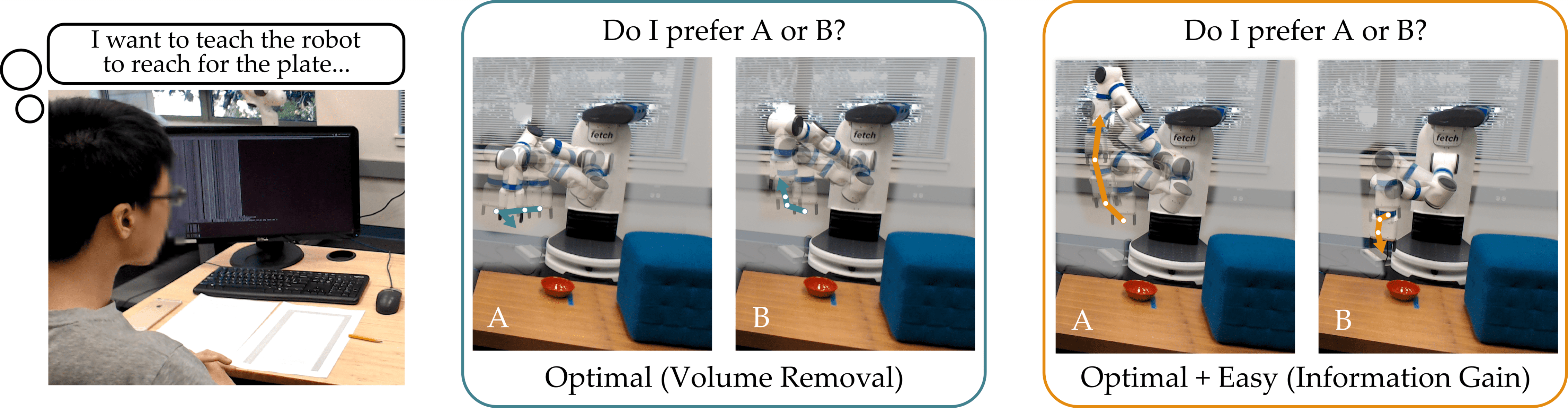
Figure 1: Comparing questions that naïvely minimize model uncertainty to queries that also account for the human’s answer uncertainty. Here the robot is attempting to learn the user’s reward function, and demonstrates two possible trajectories. The human tries to select the trajectory that better agrees with their own preferences. While the trajectories produced by volume removal are almost indistinguishable, our approach results in questions that are easy to answer: these easy questions also increase the robot’s overall learning efficiency.

2 Related Work

Reward Learning. There are many works that attempt to learn the correct reward function from human feedback. Inverse reinforcement learning (IRL) recovers the reward from expert demonstrations, where the human shows the robot how to perform the task [4, 5, 6, 7, 8]. But providing demonstrations is often difficult, particularly when the robot has many degrees of freedom [9, 10]. Preference-based learning provides a more user-friendly alternative: here the human is shown a few possible trajectories and then asked to select the best one (or rank each of them) [11, 1, 12, 13]. We are interested in leveraging preference-based learning while choosing the queries intelligently, so that we improve data efficiency and user experience.

Active Learning. Active learning seeks to tackle the data inefficiency by selecting the most informative queries, so that the robot learns as much as possible from only a few questions [14]. Recent research has applied it to preference-based learning using various optimization objectives to select the queries [12, 15, 16, 1]. Maximizing the volume removed from the hypothesis space (i.e., volume removal) is a popular approach [1, 17, 13, 18, 19, 3, 20]. Outside of preference-based learning, active learning papers approximately maximize the information gained from each question (i.e., information gain) [21, 22, 23, 24, 25, 26]. We build on both, with a focus on asking easy questions.

User-Friendly Questions. Related works found that robots which ask difficult questions can frustrate the user [11, 27], humans want to be able to express uncertainty [28], and that there is an inherent cost when asking questions (i.e., time, effort). There are some papers that attempt to address these challenges by asking natural questions [29, 30], incorporating an additional “About Equal” option to express uncertainty [31, 32, 33], or identifying the optimal time to stop asking questions [34]. Our approach incorporates all three of these challenges to ask the right number of easy questions.

3 Problem Formulation

Model. We consider a deterministic, fully-observable dynamical system. We use $s_{t}\in\mathcal{S}$ to denote the state of the system and $a_{t}\in\mathcal{A}$ to denote the action (control input) to the system, both at time $t$. A trajectory, $\xi\in\Xi$, is a finite sequence of states and actions. i.e., $\xi=((s_{t},a_{t}))_{t=0}^{T}$, where $T$ is the time horizon of the system. Since the system is deterministic, a trajectory $\xi$ can be more succinctly represented by $\Lambda=(s_{0},a_{0},a_{1},\ldots,a_{T})$, the initial state and sequence of actions in the trajectory. We use $\xi$ and $\Lambda$ interchangeably when referring to a trajectory, depending on the context.

We assume a reward function, $R:\Xi\to\mathbb{R}$, describes how a human wants the system to behave. Our goal is to learn $R$. More formally, let $R$ be a linear combination of selected features $\Phi:\Xi\to\mathbb{R}^{d}$, so that $R(\xi)=\omega^{\top}\Phi(\xi)$. To learn $R$, we simply have to learn the human’s $\omega$.

Preference Queries. A preference query $Q:=\{\xi_{1},\xi_{2},\hbox to10.00002pt{.\hss.\hss.},\xi_{K}\}$ is a set of $K$ trajectories; the human responds to a preference query by picking their most preferred trajectory from this set. We will learn the reward parameter $\omega$ by choosing—and having the human respond to—a sequence of queries.

We want to find the true reward parameter using as few preference queries as tractably possible. In other words, we want to find the sequence of queries that maximizes the amount of information that we expect to receive about $\omega$. Such a sequence of queries should recognize there is a human-in-the-loop; it should also generate queries that are “easy” for the human, thereby minimizing the amount of bad feedback it may receive. Unfortunately, this problem is, in general, NP-hard [35].

We therefore proceed in a greedy fashion: we first initialize a distribution over $\omega$, and then iteratively alternate between (a) generating a single query and (b) using the human’s response to that query to update our distribution over $\omega$. For some query generation strategies, such as the maximum volume removal method (see Sec. 4), this greedy approach has bounded regret [1].

We first focus on the second step: updating our distribution over $\omega$ based on the human’s response. Let $P(q\mid Q,\omega)$ denote the probability that the human chooses trajectory $q$ from the query $Q$ when their reward parameter is $\omega$ (see Section 7.1 for common human choice models). Then, given a prior $p(\omega)$ and the human’s response $q$ to the query $Q$, we can compute a posterior over $\omega$:

$$P(\omega\mid Q,q)\propto P(q\mid Q,\omega)P(\omega).$$

In the next sections, we discuss methods for generating the queries $Q$ that the human will answer.

4 Volume Removal Solution

Maximizing volume removal is one popular strategy for selecting queries. The method attempts to generate the most-informative queries by finding the query that maximizes the expected difference between the prior and unnormalized posterior [1, 13, 3, 18]. Formally, the method generates a query of $K$ trajectories (for $K\geq 2$) at iteration $n$ by solving:

$$Q^{*}_{n} =\operatornamewithlimits{arg\,max}_{Q_{n}=\{\Lambda_{1},\dots,\Lambda_{K}\}}\mathbb{E}_{q_{n}}\mathbb{E}_{\omega}\left[1-P(q_{n}\mid Q_{n},\omega)\right].$$ (1)

The distribution over $\omega$ can get very complex and thus—to tractably compute the expectation—we are forced to resort to sampling. Letting $\Omega$ denote a set of $M$ samples from the prior $P(\omega)$ and $\stackrel{{\scriptstyle\boldsymbol{\cdot}}}{{=}}$ denote asymptotic equality as $M\to\infty$, the optimization problem can be re-written as:

$$Q^{*}_{n}\stackrel{{\scriptstyle\boldsymbol{\cdot}}}{{=}}\operatornamewithlimits{arg\,min}_{Q_{n}=\{\Lambda_{1},\dots,\Lambda_{K}\}}\sum_{q_{n}\in Q_{n}}\left(\sum_{{\omega}\in\Omega}P(q_{n}\mid Q_{n},{\omega})\right)^{2}.$$ (2)

Failure Case. Although prior works have shown that volume removal works well in practice, here we reveal that the optimization problem used to identify volume removal queries does not capture our original goal of generating informative queries. Specifically, the trivial query, which outputs $K$ identical trajectories as options, is in fact a global solution to the volume removal formulation.

Theorem 1.

The trivial query, $Q\!=\!\{\xi_{A},\xi_{A},\hbox to10.00002pt{.\hss.\hss.},\xi_{A}\}$ (for any $\xi_{A}\in\Xi$) is the global solution to (1).

Proof.

For a given $Q$ and $\omega$, $\sum_{q}P(q\!\mid\!Q,\omega)\!=\!1$. Thus, we can bound the objective in $\eqref{eq:og_old_optimization}$ as follows:

$$\mathbb{E}_{q_{n}}\mathbb{E}_{\omega}[1-P(q_{n}\mid Q_{n},\omega)]=1-\mathbb{E}_{w}\sum_{q_{n}\in Q_{n}}P(q_{n}\mid Q_{n},\omega)^{2}\leq 1-1/K.$$

For the trivial query $Q\!=\!\{\xi_{A},\xi_{A},\hbox to10.00002pt{.\hss.\hss.},\xi_{A}\}$, the objective in (1) has value $\mathbb{E}_{q_{n}}\mathbb{E}_{\omega}\left[1\!-\!P(q_{n}\mid Q,\omega)\right]\!=\!1\!-\!1/K$, equal to the upper bound on the objective and thus, it is a global solution to (1). ∎

The robot should ask questions to learn the human’s preferences: but when all answer options are the same, the robot gains no information at all about what the human prefers! Hence, the maximum volume removal method works well in practice not despite the non-convexity of the optimization problem, but because of it. This non-convexity allows solution methods to converge to other locally optimal queries, which may be more informative than the globally optimal trivial query.

Hard Queries. Even when volume removal identifies queries that are not identical, the questions it asks may still be very challenging for the user to answer [3]. Here we provide a concrete example:

Example 1.

Let the robot query the human while providing two answer options, $q_{1}$ and $q_{2}$. First, consider a query $Q_{A}$ such that $P(q_{1}\!\mid\!Q_{A},\omega)\!=\!P(q_{2}\!\mid\!Q_{A},\omega)\ \forall\omega\!\in\!\Omega$. Intuitively, responding to $Q_{A}$ is “hard” for the human, since their probability of selecting either option is equal. Alternatively, consider a query $Q_{B}$ such that $P(q_{1}\!\mid\!Q_{B},\omega)\!\approx\!1\ \forall\omega\!\in\!\Omega^{(1)}$ and $P(q_{2}\!\mid\!Q_{B},\omega)\!\approx\!1\ \forall\omega\!\in\!\Omega^{(2)}$, where $\Omega^{(1)}\!\cup\!\Omega^{(2)}\!=\!\Omega$ and $\lvert\Omega^{(1)}\rvert\!=\!\lvert\Omega^{(2)}\rvert$. If the true $\omega$ lies in $\Omega^{(1)}$, the human will always select $q_{1}$ and conversely, if the true $\omega$ lies in $\Omega^{(2)}$, the human will always select $q_{2}$. Intuitively, this query is “easy” for the human: regardless of their true reward, the choice is almost certain.

An intelligent robot should select $Q_{B}$ over $Q_{A}$: not only does $Q_{A}$ fail to provide information about the human’s reward (because their answer could be explained by any $\omega$), but it is also hard for the human to answer (since both options seem equal). When maximizing volume removal, however, the robot thinks $Q_{A}$ is just as good as $Q_{B}$: they are both global solutions to its optimization problem. Fig. 2 demonstrates hard queries generated by the volume removal formulation.

5 Information Gain Solution

In this section we outline an alternate objective that robots should use to select useful questions. We focus on addressing the short-comings of volume removal by introducing a trade-off: instead of naïvely optimizing to minimize the robot’s uncertainty, the robot should also consider the human’s ability to answer. We find we can utilize information gain to incorporate this trade off, encouraging the robot to ask easy but informative queries. Moreover, we demonstrate that leveraging information gain to select queries has the same benefits as volume removal without its potential drawbacks.

Let us first introduce our method. At each step, we attempt to find the query that maximizes the expected information gain about $\omega$. We can do so by solving the following optimization problem:

$$Q^{*}_{n} =\operatornamewithlimits{arg\,max}_{Q_{n}=\{\Lambda_{1},\dots,\Lambda_{K}\}}I(\omega;q_{n}\mid Q_{n})=\operatornamewithlimits{arg\,max}_{Q_{n}=\{\Lambda_{1},\dots,\Lambda_{K}\}}H(\omega\mid Q_{n})-\mathbb{E}_{q_{n}}H(\omega\mid q_{n},Q_{n}),$$ (3)

where $I$ is the mutual information and $H$ is Shannon’s information entropy [36]. By approximating the expectations via sampling, we re-write this optimization problem as:

$$Q^{*}_{n} \stackrel{{\scriptstyle\boldsymbol{\cdot}}}{{=}}\operatornamewithlimits{arg\,max}_{Q_{n}=\{\Lambda_{1},\dots,\Lambda_{K}\}}\frac{1}{M}\sum_{q_{n}\in Q_{n}}\sum_{{\omega}\in\Omega}P(q_{n}\mid Q_{n},{\omega})\log_{2}{\left(\frac{M\cdot P(q_{n}\mid Q_{n},{\omega})}{\sum_{\omega^{\prime}\in\Omega}P(q_{n}\mid Q_{n},\omega^{\prime})}\right)}.$$ (4)

Robots that solve (4) to select their questions do not show identical trajectories to the user: the trivial query $Q=\{\xi_{A},\ldots,\xi_{A}\}$ is not the global solution to our new optimization problem. Instead, such a query is the actually global minimum. Additionally, the complexity of computing objective (4) is equivalent (in order) to the maximum volume removal objective (2). Thus, while being at least as tractable, our method avoids the failure case of the volume removal formulation (Theorem 1).

5.1 Generating Easy Queries

Unlike volume removal, our information gain formulation reasons over the trade-off between two sources of uncertainty: robot and human. To see this, we re-write the optimization problem as:

$$Q^{*}_{n} =\operatornamewithlimits{arg\,max}_{Q_{n}=\{\Lambda_{1},\dots,\Lambda_{K}\}}H(q_{n}\mid Q_{n})-\mathbb{E}_{\omega}H(q_{n}\mid\omega,Q_{n}).$$ (5)

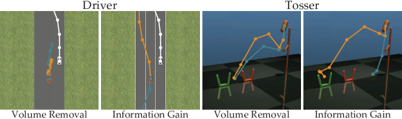
Figure 2: Sample queries generated with the volume removal and information gain methods on 2 different tasks. Volume removal generates queries that are difficult, because the options are almost equally good.

Here, the first term is the robot’s uncertainty over the human’s response: i.e., how well can the robot predict what the human will answer. The second term is the human’s uncertainty when answering: i.e., given that the user has reward parameter $\omega$, how confidently does she choose option $q$? Optimizing for information gain, without any additional easiness term, considers both types of uncertainty, and favors questions where (a) the robot is unsure how the human will answer but (b) the human can answer easily. We visualize some example queries produced by information gain in Figs. 1 and 2. We also concretely show our objective favors easy queries by returning to Example 1 from Sec. 4.

Example 2.

The first term in Eq. (5) has the same value for both $Q_{A}$ and $Q_{B}$. However, $Q_{A}$ attains the global maximum of the second term while $Q_{B}$ attains the global minimum! Thus, the overall value of $Q_{B}$ is higher and, as desired, the robot recognizes that $Q_{B}$ is a more intelligent question.

5.2 Theoretical Guarantees

When comparing our method to volume removal, we avoid its two pitfalls of identical options (Theorem 1) and difficult questions (Example 1). But we also inherit many of the same benefits, including an assurance that greedy optimization leads to bounded regret. Recall that—for both volume removal and information gain—the robot selects its question without considering the future questions. Sadigh et al. [1] have demonstrated, by virtue of the maximum volume removal objective being submodular, this greedy algorithm is guaranteed to have bounded sub-optimality in terms of the volume removed. Our method is greedy as well, and below we show it enjoys similar theoretical guarantees.

Theorem 2.

We assume that the queries are generated from a finite set and we ignore any errors due to sampling. Then, the sequence of queries generated according to (4) at each iteration is at least $1-\epsilon$ times as informative as the optimal sequence of queries after $\log\frac{1}{\epsilon}$ as many iterations.

Proof.

In Eq. (4), we aim to maximize the mutual information between $\omega$ and the set of queries $S$, which is monotone in $S$. Recall that the mutual information is a submodular function. Therefore, our objective is a submodular, monotone function, and the desired result follows directly from [37]. ∎

5.3 Extensions

Building off the volume removal method, many extensions have been developed such as batch optimization [13, 38] or warm starting techniques [3]. These extensions are agnostic to the details of the optimization; they simply require the query generation algorithm operates in a greedy manner and maintains a distribution over $\omega$. Hence, these extensions can be readily applied to our method.

Thus, when compared to the maximum volume removal, our method (1) has the same theoretical guarantees; (2) has the same computational complexity; (3) does not have a fundamental failure case; (4) generates easier queries for the human to respond; and (5) can leverage the same extensions.

6 Optimal Stopping

In the previous section, we showed how to improve the preference-based learning by easy and informative questions. We now further improve user-experience with an automatic stopping criterion: the active learning should end when the robot’s questions get more costly than they are informative.

We first extend the preference-based learning framework so that each query $Q$ has an associated cost $c(Q)$. This function captures the cost of a question: the amount of time it takes for the human to answer, the number of similar questions that the human has already seen, or even the interpretability of the question itself. We next subtract this cost from our information gain objective (3), so that the robot maximizes information gain while biasing its search towards low-cost questions:

$$r^{*}_{n}=\max_{Q_{n}=\{\Lambda_{1},\dots,\Lambda_{K}\}}I(\omega;q_{n}\mid Q_{n})-c(Q_{n}).$$ (6)

Now that we have introduced a cost into the query selection problem, the robot can reason about when its questions are becoming prohibitively expensive or redundant. Intuitively, the robot should stop asking questions if their cost outweighs their value; and, indeed, that is the optimal stopping condition when the robot maximizes information gain.

Theorem 3.

A robot using information gain to perform active preference-based learning should stop asking questions if and only if the global solution to (6) is negative at the current timestep.

The proof of the result is presented in the Appendix.

The decision to terminate our learning algorithm is straightforward: at each timestep, if $r^{*}_{n}$ is non-negative, we ask the human to respond to another query; otherwise, the robot stops asking questions. This automatic stopping procedure helps make the active learning process more user-friendly by ensuring that the user does not have to respond to any unnecessary or redundant queries.

7 Experiments

We argue that our information gain approach for asking easy questions is not only user-friendly, but also improves the robot’s learning rate. In this section we experimentally compare volume removal and information gain: we begin in Sec. 7.1 by defining how the robot models the user, and then we review our results across simulated environments (Sec. 7.2) and a user study (Sec. 7.3).

7.1 Human Choice Model

Standard Model. We require a probabilistic model for the human’s choice $q$ in a query $Q$ conditioned on their reward parameters $\omega$. Previous work demonstrated the importance of modeling imperfect human responses [39]. We model a noisily rational human as selecting $\xi_{k}$ from $Q$ by

$$P(q=\xi_{k}\mid Q,\omega) =\frac{\exp(R(\xi_{k}))}{\sum_{\xi\in Q}\exp(R(\xi))}.$$ (7)

This model, backed by neuroscience and psychology [40, 41, 42, 43], is routinely used [18, 33, 44].

Extended Model. We generalize this preference model to include an “About Equal” option for queries between two trajectories. We denote this option by $\Upsilon$ and define a weak preference query (as opposed to strict preference queries) $Q^{+}:=Q\cup\{\Upsilon\}$ when $K=2$.

Building on prior work [32], we incorporate the information from the “About Equal” option by introducing a minimum perceivable difference parameter $\delta\geq 0$, and defining:

$$P(q=\Upsilon\mid Q^{+},\omega) =\left(\exp(2\delta)-1\right)P(q=\xi_{1}\mid Q^{+},\omega)P(q=\xi_{2}\mid Q^{+},\omega)\>,$$

$$P(q=\xi_{k}\mid Q^{+},\omega) =\frac{1}{1+\exp(\delta+R(\xi_{k^{\prime}})-R(\xi_{k}))},\forall\xi_{k},\xi_{k^{\prime}}\in Q^{+}\setminus\{\Upsilon\},k\neq k^{\prime}.$$ (8)

Notice that Eq. (8) reduces to Eq. (7) when $\delta=0$; in which case we model the human as always perceiving the difference in options. All derivations in earlier sections hold with weak preference queries. In particular, we include a discussion of extending our formulation to the case where $\delta$ is user-specific and unknown in the Appendix. The additional parameter causes no trouble in practice.

We note that there are alternative choice models compatible with our framework for weak preferences (e.g., [11]). Additionally, one may generalize the weak preference queries to $K>2$, though it complicates the choice model as the user must specify which of the trajectories create uncertainty.

7.2 Simulations

We perform experiments in a variety of environments: (1) a linear dynamical system (LDS) with six-dimensional state and three-dimensional action space; (2) A two-dimensional Driver environment [45] which simulates an autonomous car with steering, braking and acceleration capabilities driving in an environment with another vehicle; (3) A Tosser robot built in MuJoCo [46] that tosses capsule-shaped object into baskets; (4) A Fetch mobile manipulator robot [47] (using OpenAI Gym [48] for simulation) that performs a reaching task among obstacles. Fig. 2 visualizes Driver and Tosser.

Implementation. We adopt the features and action spaces from [38] (detailed in Appendix). We normalize features to have unit variance under uniformly random actions. We set $K\!=\!2$, and when using the “About Equal” option set $\delta\!=\!1$. To accelerate query generation, we generate $500,000$ queries with uniformly random actions and optimize over this finite set. To judge convergence of inferred reward parameters to true parameters, we adopt the alignment metric from [1], $m\!=\!\frac{1}{M}\sum_{\bar{\omega}\in\Omega}\frac{\omega^{\top}\bar{\omega}}{\lVert\omega\rVert_{2}\lVert\bar{\omega}\rVert_{2}}$ with $M\!=\!100$, and $\Omega$ sampled using Metropolis-Hastings algorithm.

Hypothesis 1. Information gain formulation outperforms volume removal w.r.t. data-efficiency.

We sample $100$ reward parameters uniformly at random from $\{\omega\!\in\!\mathbb{R}^{d}\!\mid\!\lVert\omega\rVert_{2}\!=\!1\}$. We learn the reward functions via both strict and weak preference queries, using simulated responses. Fig. 3 shows the alignment value against query number for the $4$ different tasks. Even though the “About Equal” option improves the performance of volume removal by preventing $Q=\{\xi_{A},\xi_{A},\dots\}$ from being a global optimum, information gain gives a significant improvement on the learning rate both with and without the “About Equal” option in all environments. These results strongly support H1.

Hypothesis 2. Information gain queries are easier than those from volume removal.

The numbers given within Fig. 4 count the wrong answers and “About Equal” choices made by the simulated users. The information gain formulation significantly improves over volume removal and is slightly better than uniformly random querying. Moreover, weak preference queries consistently decrease the number of wrong answers, which can be one reason why it performs better than strict queries. Fig. 4 also shows when the wrong responses are given. While wrong answer ratios are higher with volume removal formulation, it can be seen that information gain reduces wrong answers especially in early queries, which leads to faster learning. These results support H2.

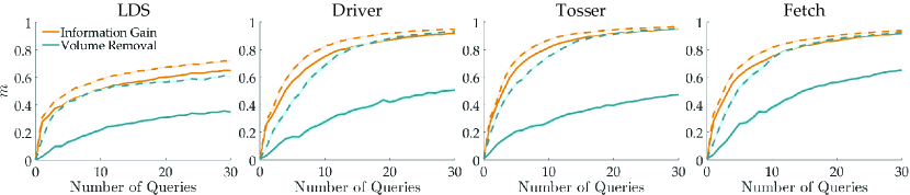
Figure 3: Alignment values are plotted (mean$\pm$s.e.). Dashed lines show the weak preference query variants.

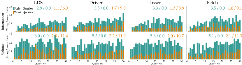
Figure 4: Wrong answer ratios on different queries are shown. The numbers at top show the average number of wrong responses and “About Equal” choices, respectively, for both strict and weak queries.

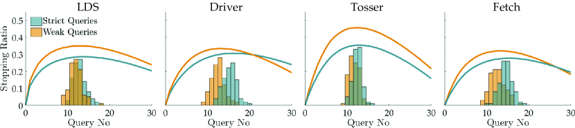
Figure 5: Simulation results for optimal stopping. Line plots show cumulative active learning rewards, averaged over $100$ test runs and scaled for visualization. Histograms show when optimal stopping condition is satisfied.

Hypothesis 3. Optimal stopping enables cost-efficient reward learning under various costs.

Lastly, to test H3, we adopted a cost to improve interpretability of queries, which may have the associated benefit of making learning more efficient [10]. We defined a cost function:

$$c(Q)=\epsilon-\lvert\Psi_{i^{*}}\rvert+\max_{j\in\{1,\dots,d\}\setminus\{i^{*}\}}\lvert\Psi_{j}\rvert,\>i^{*}=\operatornamewithlimits{arg\,max}_{i}{\lvert\Psi_{i}\rvert},$$ (9)

where $Q=\{\xi_{1},\xi_{2}\}$ and $\Psi=\Phi(\xi_{1})-\Phi(\xi_{2})$. This cost favors queries in which the difference in one feature is larger than that between all other features. Such a query may prove more interpretable. We first simulate $100$ random users and tune $\epsilon$ accordingly: For each simulated user, we record the $\epsilon$ value that makes the objective zero in the $i^{\textrm{th}}$ query (for smallest $i$) such that $m_{i},m_{i-1},m_{i-2}\in[x,x+0.02]$ for some $x$. We then use the average of these $\epsilon$ values for our tests with $100$ different random users. Fig. 5 shows the results. Optimal stopping rule enables terminating the process with near-optimal cumulative active learning rewards in all environments, which supports H3.

7.3 User Studies

We deployed our algorithm on a Fetch robot, as well as Driver and Tosser simulations. We recruited $15$ participants for the simulations and $12$ for the Fetch. We used strict preference queries; other parameters were the same as in simulations. We slightly simplified Fetch feature space and trajectories; see Appendix for details. A video demonstration is available at http://youtu.be/JIs43cO_g18.

Methodology. We began by asking participants to rank a set of features (described in plain language) to encourage each user to be consistent in her preferences. Subsequently, we queried each participant with a sequence of 30 questions generated actively; 15 from volume removal and 15 via information gain. We prevent bias by randomizing the sequence of questions for each user and experiment: the user does not know which algorithm generates a question. We test two hypotheses.

Hypothesis 4. Users find information gain queries easier than those of volume removal.

Participants responded to a 7-point Likert scale survey after each question: “It was easy to choose between the trajectories that the robot showed me.” (7-Agree, 1-Disagree). They were also asked the Yes/No question: “Can you tell the difference between the options presented?”

Figure 6 (a) shows the results of the easiness surveys. In all environments, users found information gain queries easier; the results are statistically significant (two-sample $t$-test, $p<0.005$). Fig. 6 (b) shows the average number of times the users stated they cannot distinguish the options presented. The volume removal formulation yields several queries that are indistinguishable to the users while the information gain avoids this issue. The difference is significant for Driver (paired-sample $t$-test, $p<0.05$) and Tosser ($p<0.005$). Taken together, these results support H4.

Hypothesis 5. A user’s preference aligns best with reward parameters learned via information gain.

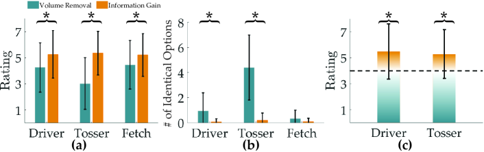
Figure 6: User study results. Error bars show std. Asterisks show statistical significance. (a) Easiness survey results averaged over all queries and users. (b) The number of identical options in the experiments averaged over all users. (c) Final preferences averaged over the users. $7$ means the user strongly prefers the optimized trajectory w.r.t. the learned reward by the information gain formulation, and $1$ is the volume removal.

In concluding the Tosser and Driver experiments, we showed participants two trajectories: one optimized using reward parameters from information gain (trajectory A) and one optimized using reward parameters from volume removal (trajectory B). Participants responded to a 7-point Likert scale survey: “Trajectory A better aligns with my preferences than trajectory B” (7-Agree, 1-Disagree).

Fig. 6(c) shows survey results. Users significantly preferred the information gain trajectory over that of volume removal in both environments (one-sample $t$-test, $p<0.05$), supporting H5.

8 Conclusion

Summary. We demonstrate robots can generate both informative and easy queries for reward learning by greedily maximizing their information gain. This objective trades-off between the uncertainties of the robot and the human about the human’s response. We also use optimal stopping to decide when questions become prohibitively expensive. Both in simulation and in a user study we demonstrate the benefits of asking the right number of easy questions. We found our formulation to be more data-efficient and generate easier (as judged by humans) queries than state-of-the-art methods.

Limitations and Future Work. To identify which questions the human can confidently answer, we rely on a cognitive model of the human. Our approach is limited by the accuracy of this model: in future work, we are interested in learning and personalizing this model for the current user. Moreover, it may be sometimes desirable to make some questions explicitly easier. One can use the interpretability cost (Eq. (9)), or add a weight term to Eq. (5) for which further research is warranted.

Acknowledgments

This work is supported by FLI grant RFP2-000 and NSF Award #1849952. Toyota Research Institute (TRI) provided funds to assist the authors with their research but this article solely reflects the opinions and conclusions of its authors and not TRI or any other Toyota entity.

9 Appendix

9.1 Derivation of Information Gain Solution

$$Q^{*}_{n} =\operatornamewithlimits{arg\,max}_{Q_{n}=\{\Delta_{1},\dots,\Delta_{K}\}}I(q_{n};\omega\mid Q_{n})$$

$$I(q_{n} ;\omega\mid Q_{n})$$

$$=H(\omega\mid Q_{n})-\mathbb{E}_{q_{n}\mid Q_{n}}\left[H(\omega\mid q_{n},Q_{n})\right]$$

$$=-\mathbb{E}_{\omega\mid Q_{n}}\left[\log_{2}\left(P(\omega\mid Q_{n})\right)\right]+\mathbb{E}_{\omega,q_{n}\mid Q_{n}}\left[\log_{2}\left(P(\omega\mid q_{n},Q_{n})\right)\right]$$

$$=\mathbb{E}_{\omega,q_{n}\mid Q_{n}}\left[\log_{2}\left(P(\omega\mid q_{n},Q_{n})\right)-\log_{2}\left(P(\omega\mid Q_{n})\right)\right]$$

$$=\mathbb{E}_{\omega,q_{n}\mid Q_{n}}\left[\log_{2}\left(P(q_{n}\mid Q_{n},\omega)\right)-\log_{2}\left(P(q_{n}\mid Q_{n})\right)\right]$$

$$=\mathbb{E}_{\omega,q_{n}\mid Q_{n}}\left[\log_{2}\left(P(q_{n}\mid Q_{n},\omega)\right)-\log_{2}\left(\int P(q_{n}\mid Q_{n},\omega^{\prime})P(\omega^{\prime}\mid Q_{n})d\omega^{\prime}\right)\right]$$

$$\stackrel{{\scriptstyle\boldsymbol{\cdot}}}{{=}}\mathbb{E}_{\omega,q_{n}\mid Q_{n}}\left[\log_{2}\left(P(q_{n}\mid Q_{n},\omega)\right)-\log_{2}\left(\frac{1}{M}\sum_{\omega^{\prime}\in\Omega}P(q_{n}\mid Q_{n},\omega^{\prime})\right)\right]$$

$$=\mathbb{E}_{\omega,q_{n}\mid Q_{n}}\left[\log_{2}\left(\frac{M\cdot P(q_{n}\mid Q_{n},\omega)}{\sum_{\omega^{\prime}\in\Omega}P(q_{n}\mid Q_{n},\omega^{\prime})}\right)\right]$$

$$=\mathbb{E}_{\omega\mid Q_{n}}\left[\mathbb{E}_{q_{n}\mid Q_{n},\omega}\left[\log_{2}\left(\frac{M\cdot P(q_{n}\mid Q_{n},\omega)}{\sum_{\omega^{\prime}\in\Omega}P(q_{n}\mid Q_{n},\omega^{\prime})}\right)\right]\right]$$

$$=\mathbb{E}_{\omega\mid Q_{n}}\left[\sum_{q_{n}\in Q_{n}}P(q_{n}\mid Q_{n},\omega)\log_{2}\left(\frac{M\cdot P(q_{n}\mid Q_{n},\omega)}{\sum_{\omega^{\prime}\in\Omega}P(q_{n}\mid Q_{n},\omega^{\prime})}\right)\right]$$

$$\stackrel{{\scriptstyle\boldsymbol{\cdot}}}{{=}}\frac{1}{M}\sum_{q_{n}\in Q_{n}}\sum_{\bar{\omega}\in\Omega}P(q_{n}\mid Q_{n},\bar{\omega})\log_{2}\left(\frac{M\cdot P(q_{n}\mid Q_{n},\bar{\omega})}{\sum_{\omega^{\prime}\in\Omega}P(q_{n}\mid Q_{n},\omega^{\prime})}\right)$$

where the integral is taken over all possible values of $\omega$.

9.2 Proof of Theorem 3

Theorem 3.

Terminating the algorithm is optimal if and only if global solution to (6) is negative.

Proof.

We need to show if the global optimum is negative, then any longer-horizon optimization will also give negative reward in expectation. Let $Q^{*}_{n}$ denote the global optimizer. For any $k\geq 0$,

$$I( q_{n},\dots,q_{n+k};\omega\mid Q_{n},\dots,Q_{n+k})-\sum_{i=0}^{k}c(Q_{n+i})$$

$$=I(q_{n};\omega\mid Q_{n})\!+\!\hbox to10.00002pt{.\hss.\hss.}\!+\!I(q_{n+k};\omega\mid q_{n},\hbox to10.00002pt{.\hss.\hss.},q_{n+k-1},Q_{n},\hbox to10.00002pt{.\hss.\hss.},Q_{n+k})\!-\!\sum_{i=0}^{k}c(Q_{n+i})$$

$$\leq I(q_{n};\omega\mid Q_{n})\!+\!\hbox to10.00002pt{.\hss.\hss.}\!+\!I(q_{n+k};\omega\mid Q_{n+k})\!-\!\sum_{i=0}^{k}c(Q_{n+i})$$

$$\leq(k+1)\left[I(q_{n};\omega\mid Q^{*}_{n})-c(Q^{*}_{n})\right]<0$$

where the first inequality is due to the submodularity of the mutual information, and the second inequality is because $Q^{*}_{n}$ is the global maximizer of the greedy objective. The other direction of the proof is very clear: If the global optimizer is nonnegative, then querying $Q^{*}_{n}$ will not decrease the cumulative active learning reward in expectation, so stopping is not optimal. ∎

9.3 Extension to User-Specific and Unknown $\delta$

We now derive the information gain solution when the parameter $\delta$ of the human model we introduced in Sec. 7.1 is unknown. One can also introduce a temperature parameter $\beta$ to the softmax model such that $R(\xi_{k})$ values will be replaced with $\beta R(\xi_{k})$ in Eqs. (7) and (8). This temperature parameter is useful for setting how noisy the user choices are, and learning it can ease the feature design.

Therefore, for generality, we denote all human model parameters that will be learned as a vector $\nu$. Since our true goal is to learn $\omega$, the optimization now becomes:

$$Q_{n}^{*} =\operatornamewithlimits{arg\,max}_{Q_{n}=\{\Lambda_{1},\dots,\Lambda_{K}\}}\mathbb{E}_{\nu\mid Q_{n}}\left[I(q_{n};\omega\mid Q_{n})\right]$$

We now work on this objective as we did in Sec. 9.1:

$$\mathbb{E} {}_{\nu\mid Q_{n}}\left[I(q_{n};\omega\mid Q_{n})\right]$$

$$=\mathbb{E}_{\nu\mid Q_{n}}\left[H(\omega\mid\nu,Q_{n})-\mathbb{E}_{q_{n}\mid\nu,Q_{n}}\left[H(\omega\mid q_{n},\nu,Q_{n})\right]\right]$$

$$=\mathbb{E}_{\nu\mid Q_{n}}\left[H(\omega\mid\nu,Q_{n})\right]-\mathbb{E}_{\nu,q_{n}\mid Q_{n}}\left[H(\omega\mid q_{n},\nu,Q_{n})\right]$$

$$=-\mathbb{E}_{\nu,\omega\mid Q_{n}}\left[\log_{2}\left(P(\omega\mid\nu,Q_{n})\right)\right]+\mathbb{E}_{\nu,q_{n},\omega\mid Q_{n}}\left[\log_{2}\left(P(\omega\mid q_{n},\nu,Q_{n})\right)\right]$$

$$=\mathbb{E}_{\nu,q_{n},\omega\mid Q_{n}}\left[\log_{2}\left(P(\omega\mid q_{n},\nu,Q_{n})\right)-\log_{2}\left(P(\omega\mid\nu,Q_{n})\right)\right]$$

$$=\mathbb{E}_{\nu,q_{n},\omega\mid Q_{n}}\left[\log_{2}\left(P(q_{n}\mid\omega,\nu,Q_{n})\right)-\log_{2}\left(P(q_{n}\mid\nu,Q_{n})\right)\right]$$

$$=\mathbb{E}_{\nu,q_{n},\omega\mid Q_{n}}\!\left[\log_{2}\left(P(q_{n}\mid\omega,\nu,Q_{n})\right)\!-\!\log_{2}\left(P(\nu,q_{n}\mid Q_{n})\right)\!+\!\log_{2}\left(P(\nu\mid Q_{n})\right)\right]$$

Noting that $P(\nu\mid Q_{n})=P(\nu)$, we drop the last term because it does not involve the optimization variable $Q_{n}$. Then, the new objective is:

$$\mathbb{E}_{\nu,q_{n},\omega\mid Q_{n}}\!\left[\log_{2}\left(P(q_{n}\mid\omega,\nu,Q_{n})\right)\!-\!\log_{2}\left(P(\nu,q_{n}\mid Q_{n})\right)\right]$$

$$\stackrel{{\scriptstyle\boldsymbol{\cdot}}}{{=}}\frac{1}{M}\sum_{(\bar{\omega},\bar{\nu})\in\Omega^{+}}\sum_{q_{n}\in Q_{n}}P(q_{n}\mid\bar{\omega},\bar{\nu},Q_{n})\left[\log_{2}\left(P(q_{n}\mid\bar{\omega},\bar{\nu},Q_{n})\right)\!-\!\log_{2}\left(P(\bar{\nu},q_{n}\mid Q_{n})\right)\right]$$

where $\Omega^{+}$ is a set that contains $M$ samples from $P(\omega,\nu)$. Since $P(\bar{\nu},q_{n}\mid Q_{n})=\int P(q_{n}\mid\bar{\nu},\omega^{\prime},Q_{n})P(\bar{\nu},\omega^{\prime}\mid Q_{n})d\omega^{\prime}$ where the integration is over all possible values of $\omega$, we can write the second logarithm term as:

$$\log_{2}\left(\frac{1}{M}\sum_{\omega^{\prime}\in\Omega(\bar{\nu})}P(q_{n}\mid\bar{\nu},\omega^{\prime},Q_{n})\right)$$

with asymptotic equality, where $\Omega(\bar{\nu})$ is the set that contains $M$ samples from $P(\omega,\bar{\nu})$ with fixed $\bar{\nu}$. Note that while we can actually compute this objective, it is computationally much heavier than the case without $\nu$, because we need to take $M$ samples of $\omega$ for each $\bar{\nu}$ sample.

One property of this objective that will ease the computation is the fact that it is parallelizable. An alternative approach is to actively learn $(\omega,\nu)$ instead of just $\omega$. This will of course cause some performance loss, because we are only interested in $\omega$. However, if we learn them together, the derivation follows Sec. 9.1 by simply replacing $\omega$ with $(\omega,\nu)$, and the final optimization becomes:

$$\operatornamewithlimits{arg\,max}_{Q_{n}=\{\Lambda_{1},\dots,\Lambda_{K}\}}\frac{1}{M}\sum_{q_{n}\in Q_{n}}\sum_{(\bar{\omega},\bar{\nu})\in\Omega^{+}}P(q_{n}\mid Q_{n},\bar{\omega},\bar{\nu})\log_{2}\left(\frac{M\cdot P(q_{n}\mid Q_{n},\bar{\omega},\bar{\nu})}{\sum_{(\omega^{\prime},\nu^{\prime})\in\Omega^{+}}P(q_{n}\mid Q_{n},\omega^{\prime},\nu^{\prime})}\right)$$

Using this approximate, but computationally faster optimization, we performed additional analysis where we compare the performances of strict preference queries, weak preference queries with known $\delta$ and weak preference queries without assuming any $\delta$ (all with the information gain formulation). As in the previous simulations, we simulated $100$ users with different random reward functions. Each user is simulated to have a true delta, uniformly randomly taken from $[0,2]$. During the sampling of $\Omega^{+}$, we did not assume any prior knowledge about $\delta$, except the natural condition that $\delta\geq 0$. The comparison results are in Fig. 7. While knowing $\delta$ increases the performance as it is expected, weak preference queries are still better than strict queries even when $\delta$ is unknown. This supports the advantage of employing weak queries.

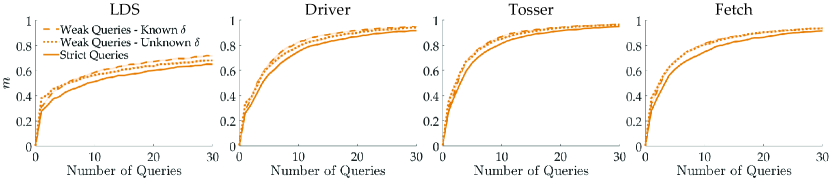
Figure 7: The simulation results with information gain formulation for unknown $\delta$. Plots are mean$\pm$s.e.

9.4 Feature Transformations and Action Spaces of the Environments

We give the details about the simulation environments in Table 1. We slightly modified the Fetch task for the user studies. We removed the average speed feature and set the robot such that it directly moves to its final position without following each of $19$ control inputs.

Table 1: Environment Details

	Driver	Tosser	Fetch (Simulations)
Features	• The average of $e^{-c_{1}d_{1}^{2}}$ over the trajectory, where $d_{1}$ is the shortest distance between the ego car and a lane center, and $c_{1}\!=\!30$. • The average of $(v_{1}\!-\!1)^{2}$ over the trajectory, where $v_{1}$ is the speed of the ego car. • The average of $\cos(\theta_{1})$ over the trajectory, where $\theta_{1}$ is the angle between the directions of ego car and the road. • The average of $e^{-c_{2}d_{2}^{2}-c_{3}d_{3}^{2}}$ over the trajectory, where $d_{2}$ and $d_{3}$ are the horizontal and vertical distances between the ego car and the other car, respectively; and $c_{2}\!=\!7$, $c_{3}\!=\!3$.	• The maximum distance the object moved forward from the tosser. • The maximum altitude of the object. • Number of flips (real number) the object does. • $e^{-c_{4}d_{4}}$ where $d_{4}$ is the final horizontal distance between the object and the center of the closest basket, and $c_{4}=3$.	• The average of $e^{-c_{5}d_{5}}$ over the trajectory where $d_{5}$ is the distance between the end effector and the goal object, and $c_{5}=1$. • The average of $e^{-c_{6}d_{6}}$ over the trajectory where $d_{6}$ is the vertical distance between the end effector and the table, and $c_{6}=1$. • The average of $e^{-c_{7}d_{7}}$ over the trajectory where $d_{7}$ is the distance between the end effector and the obstacle, and $c_{7}=1$. • The average of the end effector speed over the trajectory.
$\stackrel{{\scriptstyle\hbox{{Action}}}}{{\hbox{{Space}}}}$	The ego car is given steering and acceleration values $5$ times, each of which is applied for $10$ time steps.	The two joints of the tosser are given control inputs twice. Both the first and the second set of inputs are applied for $25$ time steps each, after the object is in free fall for $150$ time steps. In the next $800$ time steps, the user of the system observes the object’s trajectory.	The orientation of the gripper is fixed such that the end effector always points down. For the position of the gripper, we give control inputs $19$ times, each of which is applied for $8$ time steps.

9.5 Comparison of Models without Query Space Discretization

We repeated the experiment that supports H1, and whose results are shown in Fig. 3, without query space discretization. By optimizing over the continuous action space of the environments, we tested information gain and volume removal formulations with both strict and weak preference queries in LDS, Driver and Tosser tasks. We excluded Fetch again in order to avoid prohibitive trajectory optimization due to large action space. Fig. 8 shows the result. As it is expected, information gain formulation outperforms the volume removal with both preference query types. And, weak preference queries lead to faster learning compared to strict preference queries.

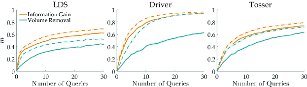
Figure 8: Alignment values are plotted (mean$\pm$s.e.). Dashed lines show the weak preference query variants.

9.6 Effect of Information from “About Equal” Responses

We have seen that weak preference queries consistently decrease wrong answers and improve the performance. However, this improvement is not necessarily merely due to the decrease in wrong answers. It can also be credited to the information we acquire thanks to “About Equal” responses.

To investigate the effect of this information, we perform two additional experiments with $100$ different simulated human reward functions with weak preference queries: First, we use the information by the “About Equal” responses; and second, we ignore such responses and remove the query from the query set to prevent repetition. We again take $M=100$ and use Metropolis-Hastings algorithm for sampling. Fig. 9 shows the results. It can be seen that for both volume removal and information gain formulations, the information from “About Equal” option improves the learning performance in Driver, Tosser and Fetch tasks, whereas its effect is very small in LDS.

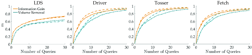
Figure 9: The results (mean$\pm$standard error) of the simulations with weak preference queries where we use the information from “About Equal” responses (dashed lines) and where we don’t use (dash-dot lines).

9.7 Optimal Stopping under Query-Independent Costs

To investigate optimal stopping performance under query-independent costs, we defined the cost function as $c(Q)=\epsilon$, which just balances the trade-off between the number of questions and learning performance. Similar to the query-dependent costs case we described in 7.2, we first simulate $100$ random users and tune $\epsilon$ accordingly: For each simulated user, we record the $\epsilon$ value that makes the objective zero in the $i^{\textrm{th}}$ query such that $m_{i},m_{i-1},m_{i-2}\in[x,x+0.02]$ for some $x$. We then use the average of these $\epsilon$ values for our tests with $100$ different random users. Fig. 10 shows the results. Optimal stopping rule enables terminating the process with near-optimal cumulative active learning rewards in all environments, which again supports H3.

Figure 10: Simulation results for optimal stopping under query-independent costs. Line plots show cumulative active learning rewards, averaged over $100$ test runs and scaled for better appearance. Histograms show when optimal stopping condition is satisfied.

References

- Sadigh et al. [2017] D. Sadigh, A. D. Dragan, S. S. Sastry, and S. A. Seshia. Active preference-based learning of reward functions. In Proceedings of Robotics: Science and Systems (RSS), July 2017.
- Cui and Niekum [2018] Y. Cui and S. Niekum. Active reward learning from critiques. In 2018 IEEE International Conference on Robotics and Automation (ICRA), pages 6907–6914. IEEE, 2018.
- Palan et al. [2019] M. Palan, G. Shevchuk, N. C. Landolfi, and D. Sadigh. Learning reward functions by integrating human demonstrations and preferences. In Proceedings of Robotics: Science and Systems (RSS), June 2019.
- Argall et al. [2009] B. D. Argall, S. Chernova, M. Veloso, and B. Browning. A survey of robot learning from demonstration. Robotics and autonomous systems, 57(5):469–483, 2009.
- Abbeel and Ng [2004] P. Abbeel and A. Y. Ng. Apprenticeship learning via inverse reinforcement learning. In Proceedings of the twenty-first international conference on Machine learning, page 1. ACM, 2004.
- Ng et al. [2000] A. Y. Ng, S. J. Russell, et al. Algorithms for inverse reinforcement learning. In Icml, volume 1, page 2, 2000.
- Abbeel and Ng [2005] P. Abbeel and A. Y. Ng. Exploration and apprenticeship learning in reinforcement learning. In Proceedings of the 22nd international conference on Machine learning, pages 1–8. ACM, 2005.
- Ziebart et al. [2008] B. D. Ziebart, A. L. Maas, J. A. Bagnell, and A. K. Dey. Maximum entropy inverse reinforcement learning. In Aaai, volume 8, pages 1433–1438. Chicago, IL, USA, 2008.
- Akgun et al. [2012] B. Akgun, M. Cakmak, K. Jiang, and A. L. Thomaz. Keyframe-based learning from demonstration. International Journal of Social Robotics, 4(4):343–355, 2012.
- Bajcsy et al. [2018] A. Bajcsy, D. P. Losey, M. K. O’Malley, and A. D. Dragan. Learning from physical human corrections, one feature at a time. In Proceedings of the 2018 ACM/IEEE International Conference on Human-Robot Interaction, pages 141–149. ACM, 2018.
- Holladay et al. [2016] R. Holladay, S. Javdani, A. Dragan, and S. Srinivasa. Active comparison based learning incorporating user uncertainty and noise. In RSS Workshop on Model Learning for Human-Robot Communication, 2016.
- Christiano et al. [2017] P. F. Christiano, J. Leike, T. Brown, M. Martic, S. Legg, and D. Amodei. Deep reinforcement learning from human preferences. In Advances in Neural Information Processing Systems, 2017.
- Biyik and Sadigh [2018] E. Biyik and D. Sadigh. Batch active preference-based learning of reward functions. In Conference on Robot Learning (CoRL), October 2018.
- Settles [2009] B. Settles. Active learning literature survey. Technical report, University of Wisconsin-Madison Department of Computer Sciences, 2009.
- Daniel et al. [2014] C. Daniel, M. Viering, J. Metz, O. Kroemer, and J. Peters. Active reward learning. In Robotics: Science and systems, 2014.
- Akrour et al. [2012] R. Akrour, M. Schoenauer, and M. Sebag. April: Active preference learning-based reinforcement learning. In Joint European Conference on Machine Learning and Knowledge Discovery in Databases, pages 116–131. Springer, 2012.
- Golovin and Krause [2011] D. Golovin and A. Krause. Adaptive submodularity: Theory and applications in active learning and stochastic optimization. Journal of Artificial Intelligence Research, 42:427–486, 2011.
- Biyik et al. [2019] E. Biyik, D. A. Lazar, D. Sadigh, and R. Pedarsani. The green choice: Learning and influencing human decisions on shared roads. In Proceedings of the 58th IEEE Conference on Decision and Control (CDC), December 2019.
- Katz et al. [2019] S. M. Katz, A.-C. L. Bihan, and M. J. Kochenderfer. Learning an urban air mobility encounter model from expert preferences. In 2019 IEEE/AIAA 38th Digital Avionics Systems Conference (DASC), September 2019.
- Basu et al. [2019] C. Basu, E. Biyik, Z. He, M. Singhal, and D. Sadigh. Active learning of reward dynamics from hierarchical queries. In Proceedings of the IEEE/RSJ International Conference on Intelligent Robots and Systems (IROS), November 2019.
- Golovin et al. [2010] D. Golovin, A. Krause, and D. Ray. Near-optimal bayesian active learning with noisy observations. In Advances in Neural Information Processing Systems, pages 766–774, 2010.
- Zheng et al. [2005] A. X. Zheng, I. Rish, and A. Beygelzimer. Efficient test selection in active diagnosis via entropy approximation. In Proceedings of the Twenty-First Conference on Uncertainty in Artificial Intelligence, pages 675–682. AUAI Press, 2005.
- Houlsby et al. [2011] N. Houlsby, F. Huszár, Z. Ghahramani, and M. Lengyel. Bayesian active learning for classification and preference learning. arXiv preprint arXiv:1112.5745, 2011.
- MacKay [1992] D. J. MacKay. Information-based objective functions for active data selection. Neural computation, 4(4):590–604, 1992.
- Krishnapuram et al. [2005] B. Krishnapuram, D. Williams, Y. Xue, L. Carin, M. Figueiredo, and A. J. Hartemink. On semi-supervised classification. In Advances in neural information processing systems, pages 721–728, 2005.
- Herbrich et al. [2003] R. Herbrich, N. D. Lawrence, and M. Seeger. Fast sparse gaussian process methods: The informative vector machine. In Advances in neural information processing systems, pages 625–632, 2003.
- Amershi et al. [2014] S. Amershi, M. Cakmak, W. B. Knox, and T. Kulesza. Power to the people: The role of humans in interactive machine learning. AI Magazine, 35(4):105–120, 2014.
- Guillory and Bilmes [2011] A. Guillory and J. A. Bilmes. Simultaneous learning and covering with adversarial noise. In ICML, volume 11, pages 369–376, 2011.
- Racca et al. [2019] M. Racca, A. Oulasvirta, and V. Kyrki. Teacher-aware active robot learning. In 2019 14th ACM/IEEE International Conference on Human-Robot Interaction (HRI), pages 335–343. IEEE, 2019.
- Cakmak and Thomaz [2012] M. Cakmak and A. L. Thomaz. Designing robot learners that ask good questions. In Proceedings of the seventh annual ACM/IEEE international conference on Human-Robot Interaction. ACM, 2012.
- Basu et al. [2018] C. Basu, M. Singhal, and A. D. Dragan. Learning from richer human guidance: Augmenting comparison-based learning with feature queries. In Proceedings of the 2018 ACM/IEEE International Conference on Human-Robot Interaction, pages 132–140. ACM, 2018.
- Krishnan [1977] K. Krishnan. Incorporating thresholds of indifference in probabilistic choice models. Management science, 23(11):1224–1233, 1977.
- Guo and Sanner [2010] S. Guo and S. Sanner. Real-time multiattribute bayesian preference elicitation with pairwise comparison queries. In Proceedings of the Thirteenth International Conference on Artificial Intelligence and Statistics, pages 289–296, 2010.
- Dimitrakakis and Savu-Krohn [2008] C. Dimitrakakis and C. Savu-Krohn. Cost-minimising strategies for data labelling: optimal stopping and active learning. In International Symposium on Foundations of Information and Knowledge Systems, pages 96–111. Springer, 2008.
- Ailon [2012] N. Ailon. An active learning algorithm for ranking from pairwise preferences with an almost optimal query complexity. Journal of Machine Learning Research, 13(Jan):137–164, 2012.
- Cover and Thomas [2012] T. M. Cover and J. A. Thomas. Elements of information theory. John Wiley & Sons, 2012.
- Nemhauser et al. [1978] G. L. Nemhauser, L. A. Wolsey, and M. L. Fisher. An analysis of approximations for maximizing submodular set functions—i. Mathematical programming, 14(1):265–294, 1978.
- Bıyık et al. [2019] E. Bıyık, K. Wang, N. Anari, and D. Sadigh. Batch active learning using determinantal point processes. arXiv preprint arXiv:1906.07975, 2019.
- Kulesza et al. [2014] T. Kulesza, S. Amershi, R. Caruana, D. Fisher, and D. Charles. Structured labeling for facilitating concept evolution in machine learning. In Proceedings of the SIGCHI Conference on Human Factors in Computing Systems, pages 3075–3084. ACM, 2014.
- Daw et al. [2006] N. D. Daw, J. P. O’doherty, P. Dayan, B. Seymour, and R. J. Dolan. Cortical substrates for exploratory decisions in humans. Nature, 441(7095):876, 2006.
- Luce [2012] R. D. Luce. Individual choice behavior: A theoretical analysis. Courier Corporation, 2012.
- Ben-Akiva et al. [1985] M. E. Ben-Akiva, S. R. Lerman, and S. R. Lerman. Discrete choice analysis: theory and application to travel demand, volume 9. MIT press, 1985.
- Lucas et al. [2009] C. G. Lucas, T. L. Griffiths, F. Xu, and C. Fawcett. A rational model of preference learning and choice prediction by children. In Advances in neural information processing systems, pages 985–992, 2009.
- Viappiani and Boutilier [2010] P. Viappiani and C. Boutilier. Optimal bayesian recommendation sets and myopically optimal choice query sets. In Advances in neural information processing systems, pages 2352–2360, 2010.
- Sadigh et al. [2016] D. Sadigh, S. Sastry, S. A. Seshia, and A. D. Dragan. Planning for autonomous cars that leverage effects on human actions. In Robotics: Science and Systems, volume 2. Ann Arbor, MI, USA, 2016.
- Todorov et al. [2012] E. Todorov, T. Erez, and Y. Tassa. Mujoco: A physics engine for model-based control. In 2012 IEEE/RSJ International Conference on Intelligent Robots and Systems, pages 5026–5033. IEEE, 2012.
- Wise et al. [2016] M. Wise, M. Ferguson, D. King, E. Diehr, and D. Dymesich. Fetch and freight: Standard platforms for service robot applications. In Workshop on Autonomous Mobile Service Robots, 2016.
- Brockman et al. [2016] G. Brockman, V. Cheung, L. Pettersson, J. Schneider, J. Schulman, J. Tang, and W. Zaremba. Openai gym. arXiv preprint arXiv:1606.01540, 2016.