Deep localization of subcellular protein structures from fluorescence microscopy images

Abstract

Accurate localization of proteins from fluorescence microscopy images is challenging due to the inter-class similarities and intra-class disparities introducing grave concerns in addressing multi-class classification problems. Conventional machine learning-based image prediction pipelines rely heavily on pre-processing such as normalization and segmentation followed by hand-crafted feature extraction to identify useful, informative, and application-specific features. Here, we demonstrate that deep learning-based pipelines can effectively classify protein images from different datasets. We propose an end-to-end Protein Localization Convolutional Neural Network (PLCNN) that classifies protein images more accurately and reliably. PLCNN processes raw imagery without involving any pre-processing steps and produces outputs without any customization or parameter adjustment for a particular dataset. Experimental analysis is performed on five benchmark datasets. PLCNN consistently outperformed the existing state-of-the-art approaches from traditional machine learning and deep architectures. This study highlights the importance of deep learning for the analysis of fluorescence microscopy protein imagery. The proposed deep pipeline can better guide drug designing procedures in the pharmaceutical industry and open new avenues for researchers in computational biology and bioinformatics.

1 Introduction

Protein subcellular localization refers to the spatial distribution of different proteins inside a cell. To understand various cellular processes, it is crucial to comprehend the functions of proteins, which are in turn highly correlated to their native locations inside the cell yang2014image ; chong2015yeast ; parnamaa2017accurate ; shao2017deep . Protein functions can be better grasped by identifying the protein subcellular spatial distributions. For instance, proteins at mitochondria perform aerobic respiration and energy production in a cell glory2007automated ; xu2018bioimage . During the drug discovery procedures, precise information about the location of proteins can also help in identifying drugs tahir2011protein . Similarly, information about the location of proteins before and after using certain drugs can reveal their effectiveness glory2007automated ; itzhak2016global . Proteins residing in different locations are dedicated to performing some particular functions, and any change in their native localizations may be a symptom of some severe disease xu2018bioimage ; xiang2019amc . Therefore, capturing the change in proteins’ native locations is significant in detecting any abnormal behavior ahead of time that may be important to some diagnostic or treatments.

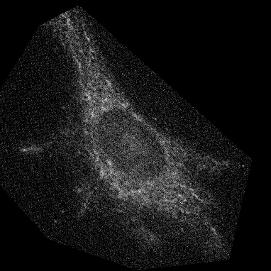
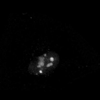
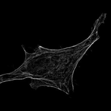
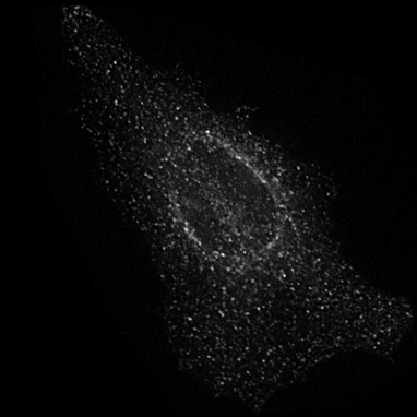
Microscopy techniques are employed to capture subcellular localization images of proteins in a cell, which were previously analyzed using traditional wet methods. However, advances in microscopy techniques have brought an avalanche of medical images in a considerable amount; hence, manual analysis and processing of these medical images become nearly impossible for biologists. Moreover, a subjective inspection of images may lead to errors in decision-making process shao2017deep ; tahir2011protein ; kreft2004automated . It is highly likely that the images generated for proteins of the same class may look visually different (see Figure 1). Similarly, proteins belonging to two different classes may look alike. Such a situation leads to the poor performance of classification systems. These problems are resolved by applying different hand-crafted feature extraction strategies to capture multiple views from the same image tahir2016protein . Hence, this is a cumbersome job and may fail to discriminate with high accuracy.

Due to the reasons mentioned above, automated computational techniques continued to focus on many researchers in computational biology and bioinformatics over the last two decades xu2018bioimage . Consequently, substantial advancement has been observed concerning the automated computational methods, improving the performance of protein subcellular localization from microscopy images.

Our primary contributions are 1): we introduce a novel architecture, which exploits different features at various levels in distinct blocks, 2): we investigate the effect of different components of the network and demonstrate improved prediction accuracy, and 3): we provide extensive evaluation on five datasets against a number of traditional and deep-learning algorithms.

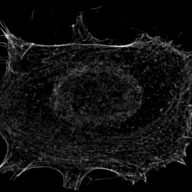
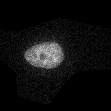
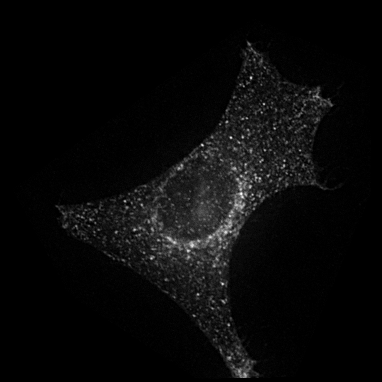
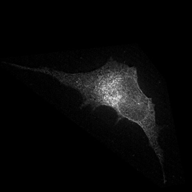
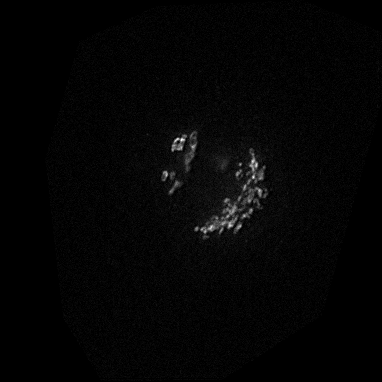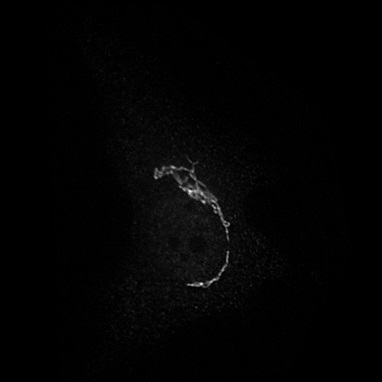
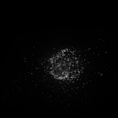
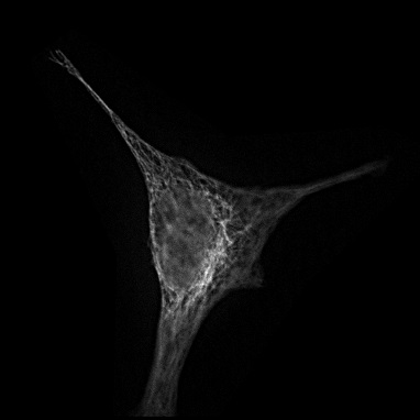
Actin DNA Endosome Endoplasmic Reti. Golgia Golgpp Lysosome Microtubule Mitochondria Nucleolus

Figure 1: Images from Hela dataset for protein localization; each image belongs to a different class. Most of the images are Sparse. Best viewed when zoomed-n on a display.

2 Related Works

Murphy’s group has instituted pioneering work in the machine learning computational methods, to accurately predict subcellular locations of proteins from fluorescence microscopy images. In this connection, Boland et al.have proposed to utilize Zernike moments and Haralick texture features in conjunction with a neural network to classify protein images from CHO dataset boland1998automated into five distinct categories. Next, as an extension to their earlier work, Murphy et al.murphy2000towards have introduced a quantitative approach in which they not only employed Zernike moments and Haralick texture features for the description of protein images but also presented a new set of geometric and morphological features. Back-propagation neural network, linear discriminator, K-nearest neighbors and classification trees were investigated for the stated purpose. Adopting the previous feature extraction techniques, Huang and Murphy huang2004boosting formed an ensemble of three classifiers to localize the subcellular proteins.

The proposed approaches by the Murphy group have demonstrated significant performance in discriminating protein localization images. However, they had to apply a number of feature extraction techniques where each technique is dedicated to capturing certain aspects of protein images. Following the works of Murphy et al., a novel feature extraction technique known as Threshold Adjacency Statistics (TAS) is proposed in hamilton2007fast , in which the input image is converted into binary images using different thresholds. In the next step, from each binary image, nine statistics are computed, which serve as an input to support vector machines (SVM) for classification. TAS is able to extract meaningful information from protein images with low computational complexity. However, appropriate threshold selection has a great impact on the performance of generated features. Moreover, Chebira et al. chebira2007multiresolution reported a multi-resolution approach using Haar filters to decompose an input image into multi-resolution subspaces, extracting Haralick, morphological, and Zernike features, and performing classification in respective multi-resolution subspaces. Results obtained in this way are combined through a weighting algorithm to yield a global prediction independently. The proposed multi-resolution approach demonstrated enhanced performance that comes at the expense of increased computational cost.

Nanni & Lumini nanni2008reliable presented the concatenated features of invariant LBP, Haralick, and TAS in conjunction with a random subspace of Levenberg-Marquardt Neural Network. LBP technique is the choice of many researchers for texture classification due to its intrinsic properties; for example, they are rotation invariant, resistant to illumination changes, and computationally efficient. Despite its simplicity, it is capable of extracting minute details from image texture. However, its noise-sensitive nature may lead to poor performance. Building on the success of LBP features, Nanni et al.nanni2010local have put forward variants of LBP for feature extraction, exploiting the topological arrangements for neighborhood calculation as well as several encoding schemes for the assessment of local gray-scale differences. The resultant features are then fed to a linear SVM for training. These variants curbed the noise-sensitive behavior of LBP that enhanced its discriminative power.

In fluorescence microscopy, Li et al. li2013automated combined the concepts from LBPs and TASs to develop a novel technique: Local Difference Patterns (LDPs), engaging SVM as a classifier. LDPs are invariant to translation and rotation that showed better performance compared to other simple techniques like Haralick features and TASs. Similar to zhang2011phenotype , Tahir and Khan tahir2016protein employed GLCM that exploits statistical and Texton features. The classification is performed through SVM, and the final prediction is obtained through the majority voting scheme. The proposed technique has shown some-how better performance through efficient exploitation of two simple methods. Moreover, Tahir et al. tahir2018efficient enhanced the discriminative power of the TAS technique by incorporating seven threshold ranges resulting in seven binary images compared to three hamilton2007fast . The seven SVMs are trained using each binarized image features, while the majority voting scheme delivers the final output. Though this technique’s performance is better than its classical counterpart, it requires the calculation of additional threshold values that make it computationally expensive.

The core issue with classical machine learning methods is identifying appropriate features for describing protein images with maximum discriminating capability and selecting proper classifiers to benefit from those features. Any single feature extraction technique usually extracts only one aspect of essential characteristics from protein images. Hence, different feature extraction strategies are applied to extract diverse information from the same image. Additionally, segmentation and feature selection may also be required to obtain more relevant and useful information from protein images, which may result in more computational cost, time, and efforts nanni2017handcrafted ; xiao2019application . In case the extracted features reasonably describe the data under consideration, it cannot be guaranteed that the same technique works for data other than the one for which it has been crafted kraus2017automated .

In recent years, convolutional neural networks (CNNs) have attracted the focus of many researchers in a variety of problem domains parnamaa2017accurate ; le2019identification ; zhang2019protein ; guo2019identification . Deep learning provides solutions to avoid cumbersome tasks related to classical machine learning problems xiao2019application ; kraus2017automated ; gu2018recent . The deep learning prediction systems learn features directly from the raw images without the need for designing and identifying hand-crafted feature extraction techniques. Similarly, in CNNs, pre-processing is not a primary requirement compared to classical prediction models.

In the field of computational biology and bioinformatics, Dürr and Sick durr2016single applied a convolutional neural network to biological images for the classification of cell phenotypes. The input to the model is a segmented cell rather than a raw image. More recently, Pärnamaa and Parts parnamaa2017accurate developed a CNN model named DeepYeast for the classification of yeast microscopy images and localization of proteins. Shao et al. shao2017deep coupled classical machine learning with CNNs for classification. In this connection, AlexNet krizhevsky2012imagenet is used to extract features from natural images, which are followed by a partial parameter transfer strategy to extract features from protein images. Next, feature selection is performed on the last fully connected layer using Lasso model tibshirani1996regression , and the resultant features were fed into RBF-SVM for final output.

To classify efficiently, Godinez et al. godinez2017multi developed a multi-scale CNN architecture that processes images at various spatial scales over parallel layers. For this purpose, seven different scaled versions are computed for each image to feed into the network. Each image is processed through three convolutional layers, establishing a convolutional pathway for each sequence, which works independently of the other and captures relevant features appearing at a particular scale. Next, Kraus et al. kraus2017automated trained DeepLoc, a convolutional neural network consisting of convolutional blocks and fully connected layers. The convolutional layers identify invariant features from the input images, while fully connected layers classify the input images based on the features computed in the convolutional layers.

Lately, Xiao et al. xiao2019application analyzed various types of deep CNNs for their performance against conventional machine learning techniques. Comparable to DeepYeast parnamaa2017accurate , Xiao et al.xiao2019application implemented 11-layer CNN with batch normalization, similar to VGG simonyan2014vgg . The authors further experimented and analyzed VGG, ResNet he2016deep , Inception-ResNet V₂ szegedy2017inception , straightened ResNet (modified version), and CapsNet sabour2017dynamic . Besides, as a separate experiment, image features are extracted using convolutional layers of VGG (employing batch normalization) and the conventional machine learning classifier replacing the last fully connected layer. The obtained results using various CNN models proved their efficiency compared to conventional machine learning algorithms. Recently, Lao & Fevens lao2019cell employed ResNet he2016deep and many of its variants for cell phenotype classification from raw imagery without performing any prior image segmentation. They demonstrated the capabilities of WRN zagoruyko2016wide , ResNeXt xie2017aggregated , and PyramidNet han2017deep .

Our method, protein localization convolutional neural network, namely, PLCNN, employs a multi-branch network with feature concatenation. Each branch of the network computes different image features due to its block structure based on distinct skip connections. Unlike traditional methods, no pre-processing or post-processing is performed to achieve favorable and data-specific results. In the next section, we provide details about our network.

3 Proposed Network

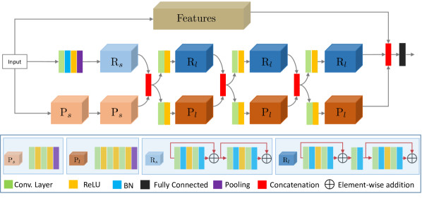
Recently, plain networks such as VGG simonyan2014vgg , residual networks such as ResNet he2016deep and densely concatenated networks such as DenseNet huang2017denseNet have delivered a state-of-the-art performance in object classification, recognition, and detection while offering the stability of the training. Inspired by the elements of mentioned networks, we design a modular network to localize protein structures in cell images. The design consists of three types of modules: 1) without any skip connections, 2) with skip connections, and 3) with dense connections. Figure 2 outlines the architecture of our network. We first provide the rationale behind our design

Design Rationale: Our purpose here is to design a network where we can exploit a novel multi-branch architecture. It has been shown in many tasks anwar2019densely that such structures help in learning different features via different strategies. Therefore, we carefully design the network keeping in mind the various approaches. We want to exploit previously learned features in the first branch, relying on the current and all previous layers’ concatenation. The network’s second branch should learn the residuals in the input image, while the last one should learn the features sequentially. We also concatenate the second and third branch features, hence reinforcing the course correction of the network. Due to these carefully designed factors, our method performs more accurately than the mentioned classification networks.

Network Elements: Our proposed network has a modular structure composed of different modules. The variation of each module is depicted via the colors employed. The orange color represents the non-residual part, and the blue blocks are for residual learning. Similarly, the golden block uses dense connections to extract features from the images. The outputs of each residual and non-residual blocks are concatenated except the first blocks. Our experiments typically employ filters of size $3\times 3$ and $1\times 1$ in the convolutional layers. Next, we explain the difference between the blocks.

Apart from the noticeable difference between the modules based upon the connection types, the modules are distinct in their composition of elements. To be more precise, our network is governed by four meta-level structures; the connection types in the modules, the number of modules, the elements in the modules, and the number of feature maps.

Our network’s high-level architecture can be regarded as a chain of modules of residual and non-residual blocks, where the concatenation happens after each block. Each concatenation’s output is fed into each convolutional layer to compress the high number of channels for computational efficiency. At the end of the network, the output features of residual, non-residual, and dense parts are stacked together, flattened, and passed through the fully connected layer to produce probabilities equal to the number of classes. The class with the highest probability is declared as the protein type present in the image.

The simplest of the three modules is the plain one, which comprises convolutional layers, each followed by ReLU and a final max-pooling operation at the end of the module. Moreover, there are two types of plain modules i.e. P_s and P_l where the difference lies in the number of convolutional layers. The former contains two, and the latter contains three layers.

The residual modules consist of two convolutions where batch normalization and ReLU follow the first one, while the second one is followed by only batch normalization. The input of the block is added to the output of the second batch normalization. This structure is repeated two times in each R_s residual module, while for R_l, a strided convolution is added between the two structures to match the size for the corresponding plain modules before concatenation. The architecture of R_s and R_l are shown in the lower part of Figure 2. Features block takes its inspiration from DenseNet huang2017denseNet , where each layer is stacked with the previous layers. These modules aim at learning the kernel weights to predict accurate probabilities. The skip connections in residual and dense modules help propagate the loss gradients without a bottleneck in the forward and backward direction.

Formulation: Let us suppose that an image $y$ is passed via a deep network having $N$ layers, where each layer implements a non-linear transformation function $M_{n}(\cdot)$ and $n$ represents the index of the layer. $M_{n}(\cdot)$ can be composed of compound operations, e.g. convolution, batch normalization, ReLU, or pooling, then the output of the $n^{th}$ layer can be denoted as $y_{n}$.

Non-Residual Modules: Non-residual convolutional networks pass the input through $n^{th}$ module to get the features of $(n+1)^{th}$ i.e. connecting the output with the input via a single feed-forward path, which gives rise to the following layer transition

$$y^{n_{r}}_{n}=M_{n}(y_{(n-1)}),$$ (1)

where $n_{r}$ represents the output of the non-residual non-linear transformation module.

Residual Modules: On the other hand, residual blocks connect the input with the output using a skip, also known as bypass, connection over $M_{n}(\cdot)$ as

$$y^{r}_{n}=M_{n}(y_{(n-1)})+y_{(n-1)},$$ (2)

where $r$ indicates features from the residual module.

Figure 2: A glimpse of the proposed network used for localization of the protein structures in the cell. The composition of R_s, R_l, P_s, and P_l are provided below the network structure, where the subscript _s has a small number of convolutions as compared to _l. The P_s and P_l are two types of plain modules, where the difference lies in the number of convolutional layers; the former contains two, and the latter contains three layers. Similarly, the R_s residual module consists of two convolutions where batch normalization and ReLU follow the first one, while the second one is followed by only batch normalization, while for R_l, a strided convolution is added between the two structures to match the size for the corresponding plain modules before concatenation.

Dense Connections: The dense modules employ dense connections, which receive features from all the previous layers as input:

$$y^{d}_{n}=M_{n}([y_{0};y_{1};y_{2};\ldots;y_{n-1}]),$$ (3)

where $[\cdot]$ represents concatenation of feature maps from layers $0,\ldots,n-1$. Similarly, $d$ refers to the output features from the dense module.

Composite Function: Inspired by he2016deep and huang2017denseNet , we also define the composite function M${}_{n}(\cdot)$ having three operations: convolution followed by batch normalization and ReLU.

Channels Compression: The number of channels is reduced after the final concatenation in the dense module and after the concatenation of the feature maps from non-residual and residual modules to improve the model compactness and efficiency.

Label Prediction: As a final step, the features of all the modules are stacked and passed through a fully connected layer after softmax produces probabilities equal to the number of classes present in the corresponding dataset. The highest probability is considered to be the predicted class as

$$\alpha=\psi(\tau([y^{d}_{f},y^{r}_{f};y^{n_{r}}_{f}])),$$ (4)

where $f$ represents the last transformation function. Similarly, $\tau$ is the fully connected operation, and $\psi$ operator selects the highest probability and maps it to the predicted class label $\alpha$.

Network Loss: The fully-connected layer’s output is fed into the softmax function, which is the generalization of the logistic function for multiple classes. The softmax normalizes the values in 0 and 1 intervals where normalized values add up to 1. The softmax can be described as

$$F(y_{i})={e^{y_{i}}}\bigg{/}{\sum_{j=1}^{n}e^{y_{j}}}$$ (5)

where $y_{i}$ represents actual values corresponding to $n$ mutually exclusive classes.

We employ cross-entropy as a loss function, which computes the difference between the predicted probabilities and the class’s actual distribution. One-hot encoding is used for the actual class distribution, where the probability of the real class is 1 and all other probabilities are zero. The cross-entropy loss is given by

Table 1: The description of parameters and symbols used in proposed algorithms.

Symbols Description Symbols Description $\Omega$ Dataset $\tau_{r}$ Training Data $S_{\Omega}$ DatasetSize $\nu$ Validation Data $\beta$ BatchSize $\rho$ Testing Data $\varepsilon$ Epochs $Conv$ Convolutional layer $N_{B}$ No. of Blocks $y_{n}$ n^th layer’s output $F(y_{i})$ Class probabilities $M_{n}(\cdot)$ Conv+BN+ReLU $\phi$ Trained Network $\alpha$ Predict class label $\tau$ Fully-Connnected $\gamma$ Learning rate $p_{i}(y)$ Actual probability $q_{i}(y)$ Estimated probability $\varepsilon_{i}=\frac{S_{\Omega}}{\beta}$ No. of Iterations per Epoch $\psi$ Probability selector

$$l(p,q)=-\sum_{i=1}^{n}p_{i}(y)\log(q_{i}(y)),$$ (6)

where $p_{i}(y)$ is the actual probability and $q_{i}(y)$ is the estimated probability of class $i$. We provide the whole process as algorithm 1 and algorithm 2 and explanations of symbols are presented in Table 1.

1:  Inputs: $\Omega$, $S_{\Omega}$, $\beta$, $\varepsilon$, $N_{B}$

2:  Output: $F(y_{i})$, $\phi$

3:  Initialization: $\varepsilon=40,\gamma=10^{-4},\beta=32,\varepsilon_{i}=\frac{S_{\Omega}}{\beta}$

4:  Data preparation: [$\tau_{r},\nu,\rho$ ] = data_split ($\Omega$) ;

 // Split dataset

5:  Training:

6:  for  p = 1 to $\varepsilon$ do

7:     for  k = 1 to $\varepsilon_{i}$ do

8:        $F(y_{i})$= $\phi$($\Omega_{k}$, $N_{B}$) ;

 // Network training (algorithm 2)

9:         Calculate $l(p,q)=-\sum_{i=1}^{n}p_{i}(y)\log(q_{i}(y))$ ;

 // Cross Entropy

10:        BackPropagate Gradients ;

 //

11:        Update Network Parameters ;

 //

12:     end for

13:  end for

14:  Testing:

15:  for  k =1 to $S_{\Omega}$ do

16:     $F(y_{i})=\phi(\Omega_{k},N_{B})$ ;

 // Network testing (algorithm 2)

17:  end for

18:  Output: $F(y_{i})$

Algorithm 1 Classification Framework

1:  Main Network Steps:

2:  Step 1: Compute Dense Features   

3:  $y^{d}_{n}=M_{n}([y_{0};y_{1};y_{2};\ldots;y_{n-1}])$ ;

 // From eq. 3

4:  Step 2: Compute Residual & Non-Residual Features

5:  for  p = 1 to $N_{B}$ do

6:     if p==1 then

7:        $n=0$ ;

 // If first layer then index is zero

8:     else

9:        $y^{n_{r}}_{n}=M_{n}(y_{(n1-1)})$ ;

 // From eq. 1

10:        $y^{r}_{n}=M_{n}(y_{(n2-1)})+y_{(n2-1)}$ ;

 // From eq. 2

11:        $y^{c}_{n}=[y^{n_{r}}_{n},y^{r}_{n}]$ ;

 // Concatenate features

12:        $y_{n1}=Conv(y^{n_{r}}_{n})$ ;

 // First Convolutional layer output

13:        $y_{n2}=Conv(y^{r}_{n})$ ;

 // Second Convolutional layer output

14:     end if

15:  end for

16:  Step 3: Concatenate Computed Features   

17:  $y_{i}=\psi(\tau([y^{d}_{f},y^{r}_{f};y^{n_{r}}_{f}]))$ ;

 // From eq. 4

18:  Step 4: Normalize outputs

19:  $F(y_{i})={e^{y_{i}}}\bigg{/}{\sum_{j=1}^{n}e^{y_{j}}}$ ;

 // From eq. 5

20:  Return: $F(y_{i})$

Algorithm 2 Protein Classification Network (PLCNN)

4 Experimental settings

First, we detail the training of our network. Subsequently, we discuss the datasets used in our experiments. These include HeLa boland2001neural , CHO boland1998automated , LOCATE datasets hamilton2007fast , and Yeast parnamaa2017accurate . Next, we evaluate our network against conventional algorithms such as SVM-SubLoc tahir2011protein , ETAS-Subloc tahir2018efficient , and IEH-GT tahir2016protein as well as convolutional neural networks such as AlexNet krizhevsky2012imagenet , ResNet he2016deep , GoogleNet szegedy2015going , DenseNet huang2017denseNet , M-CNN godinez2017multi and DeepYeast parnamaa2017accurate . In the end, we analyze various aspects of the proposed network and present ablation studies.

4.1 Training Details

During training, the input to our network are the resized images of 224$\times$224 from the corresponding datasets. Training and testing are performed via 10-fold cross-validation, and there is no overlap i.e. both are disjoint in each iteration. We also augment the training data by applying conventional techniques such as flipping horizontally and vertically as well as rotating the images within a range of $[0,\frac{\pi n}{2}]$, where $n=1,2,3$. We also normalized the images using ImageNet krizhevsky2012imagenet mean and standard deviation.

We implemented the network using the PyTorch framework and trained it using P100 GPUs via SGD optimizer ruder2016overview . The initial learning rate was fixed at $10^{-2}$ with weight decay as $10^{-4}$ and momentum parameter as $0.9$. The learning rate was halved after every 10⁵ iterations, and the system was trained for about 4$\times$10⁵ iterations. The training time was variable for each dataset; however, as an example, the training for CHO dataset boland1998automated took around 14 minutes to complete the mentioned iterations. The batch size was selected to be $32$. The residual component of the network was initialized from the weights of ResNet he2016deep , the non-residual part from VGG simonyan2014vgg , and the densely connected section from DenseNet huang2017denseNet weights.

4.2 Datasets

We analyzed the PLCNN approach’s performance on five benchmark subcellular localization datasets that are described as follows.

Table 2: Performance comparison with machine learning and CNN-Specific algorithms. The “Endo” and “Trans” is the abbreviation for LOCATE Endogenous and Transfected datasets, respectively. Best results are highlighted in bold.

Method HeLa CHO Endo Trans Yeast Machine Learning SVM-SubLoc 99.7 - 99.8 98.7 - ETAS-SubLoc - - 99.2 91.8 - IEH-GT - 99.7 - - - CNN Specific GoogleNet 92.0 91.0 - - - M-CNN 91.0 94.0 - - - DeepYeast - - - - 91.0 PLCNN (Ours) 93.0 100.0 99.8 99.6 91.0

Table 3: Performance against traditional CNN methods using on all the five datasets. The best results are in bold.

Methods Datasets Alexnet ResNet DenseNet Ours HeLa 85.1 86.5 87.9 93.0 CHO 97.4 98.6 98.4 100.0 Endo 98.1 99.1 99.2 99.8 Trans 94.2 98.4 98.8 99.6 Yeast 80.9 81.5 81.7 91.0

• HeLa dataset: HeLa dataset boland2001neural is a repository of 2D fluorescence microscopy images from HeLa cell lines where each organelle is stained with a corresponding fluorescent dye. Overall, there are 862 single cell images distributed in 10 different categories. Figure 3 highlights the distribution of protein images and the number of images in each class for the HeLa dataset. The number of images is given on the y-axis, while each category’s labels are on the x-axis. The largest number of images are in the Actin category, while the lowest belongs to the Mitochondria class.

  

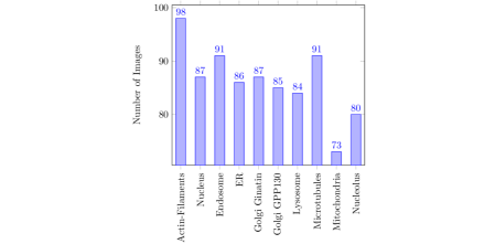
  Figure 3: HeLa Dataset: The number of images in each class. The horizontal axis shows the type of protein the images belong.

• CHO dataset: CHO dataset boland1998automated is developed from Chinese Hamster Ovary cells that contain 327 fluorescence microscopy images. Figure 4 provides an overview of the class distribution as well as the images per class in the CHO dataset. There are only five CHO classes, having the minimum number of images in Nucleolus and the maximum number in Lysosome.

  

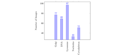
  Figure 4: CHO dataset: The five classes of the CHO dataset boland1998automated with the number of images per class.

• LOCATE datasets: LOCATE is a compilation of two datasets hamilton2007fast i.e. LOCATE Endogenous and LOCATE Transfected, each containing 502 and 553 subcellular localization images distributed in 10 and 11 classes, respectively. Figure 5 depicts the distribution of images in various categories for each dataset. The blue bars represent the images in Endogenous, while the red bars are for the Transfected dataset. The distribution of images in all the categories is mostly even.

  Figure 5: Locate dataset: The protein images of LOCATE datasets. The blue and red bars represent the Endogenous and Transfected datasets, respectively.

• Yeast dataset: We have used the Yeast dataset developed by Parnamaa & Parts parnamaa2017accurate that consists of 7132 microscopy images distributed over 12 distinct categories. To augment the original dataset, the images were cropped into 64$\times$64 patches, generating 90,000 samples in total. These patches are distributed exclusively into 65,000 training, 12,500 validation, and 12,500 testing. Only the training and testing samples per class are illustrated in Figure 6. The number of images for the Peroxisome organelle is the least, while most images are found in Cytoplasm.

  

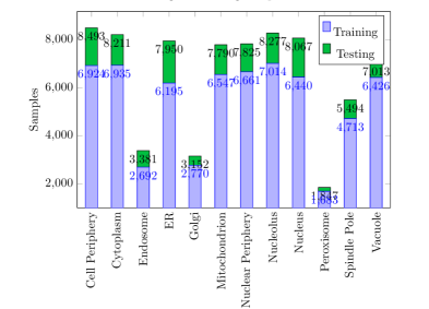
  Figure 6: Yeast dataset: Per class training and testing samples from Yeast dataset. The blue color shows the number of training images, and the dark green represents the testing images.

4.3 Comparisons

In this section, we provide comparisons against state-of-the-art algorithms on the datasets, as mentioned earlier. The proposed PLCNN results are reported without any customization or parameter adjustment for a particular dataset. We employ BBBC datasets ljosa2012BBBC , where only two types of phenotype classes are present, namely, the neutral and positive control phenotypes. During comparison on this dataset, our algorithm, as well as other deep learning methods including M-CNN godinez2017multi , achieved perfect classification. The problem on the mentioned datasets is a simple binary classification; hence, reporting results on BBBC datasets ljosa2012BBBC become trivial.

Figure 7: The average quantitative results of ten execution for each method on the HeLa dataset. Our PLCNN method consistently outperforms with a significant margin.

4.3.1 Multi class subcellular organelles classification

Groundtruth
AlexNet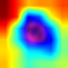
DenseNet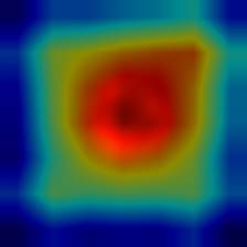
ResNet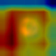
PLCNN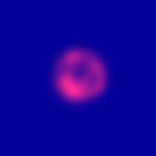

Figure 8: Visualization results from Grad-CAM selvaraju2017grad . The visualization is computed for the last convolutional outputs, and the corresponding algorithms are shown in the left column of the input images. Each method focuses on sample images from CHO and Yeast datasets. Our approach provides the best results due to the correct identification of proteins; other methods fail to focus as indicated by the random colors.

Traditional models: We present a comparative analysis of the PLCNN model against the conventional machine learning models. For a fair comparison, we train and test our network using the same dataset configuration. Table 2 highlights the performance of PLCNN and machine learning-based models. Although SVM-SubLoc tahir2011protein has achieved $99.7\%$ accuracy for HeLa dataset boland2001neural , the pre-processing requires widespread efforts and are highly time-consuming. Likewise, identifying suitable representative features is also a cumbersome job. Moreover, the SVM-SubLoc tahir2011protein , ETAS-Subloc tahir2018efficient , and IEH-GT tahir2016protein are ensemble methods i.e. combination of multiple traditional classification algorithms; that is why, the performances are higher than many of the complex systems nanni2008reliable ; nanni2010selecting ; lin2007boosting for HeLa and CHO datasets.

Tahir et al. tahir2011protein captured multi-resolution subspaces of each image before extracting features. Similarly, the model ETAS-SubLoc tahir2018efficient for the feature extraction performs extensive pre-processing to produce multiple thresholded images from a single protein image. Similarly, IEH-GT tahir2016protein has achieved $99.7\%$ performance accuracy for the CHO dataset where the authors had to employ several hand-crafted pre-processing and feature extraction steps for such efficient classification.

Comparative analysis in Table 2 reveals that PLCNN outperforms all methods on all datasets except HeLa boland2001neural even though it does not require any pre-processing. The PLCNN achieved $93.0\%$ accuracy for HeLa boland2001neural that is lower than that of SVM-SubLoc tahir2011protein ; the latter employs an ensemble of classifiers. Furthermore, the traditional algorithms tahir2011protein ; tahir2016protein are usually tailored for specific datasets and hence only perform well on particular datasets for which they are designed. These algorithms fail to deliver on other datasets, thus indicating limited generalization capability.

On the other hand, PLCNN performs well across multiple subcellular localization datasets. Mainly, LOCATE Transfected dataset has been observed to be one of the most challenging datasets where the performance of stand-alone conventional machine learning algorithms for a single feature extraction technique is below $92\%$ as demonstrated in  Conventional-nanni2018bioimage ; Conventional-nanni2019general . In order to improve the performance of conventional machine learning algorithms, researchers usually adopt the notion of ensemble methods to exploit hybrid feature spaces chong2015yeast ; chebira2007multiresolution ; zhang2011phenotype ; tahir2018efficient . In such cases, extensive efforts are required to find an effective combination of classification algorithms and discriminative feature descriptors. In contrast, PLCNN achieved $99.6\%$ accuracy on this dataset, improving upon the traditional techniques without spending huge efforts on identifying effective feature descriptors and machine learning algorithms.

Table 4: The effect of decreasing the training dataset. It can be observed that the performance decrease for traditional ensemble algorithms with the decrease in training data while, on the other hand, PLCNN gives a consistent performance with a negligible difference.

Methods Dataset Split SVM ETAS Ours CHO 90%-10% 99.6 47.0 100.0 80%-20% 99.6 50.4 99.3 70%-30% 99.3 57.1 98.9 60%-40% 98.7 86.8 99.0 Endogenous 90%-10% 99.0 98.0 99.8 80%-20% 98.8 97.8 99.7 70%-30% 95.8 96.2 99.7 60%-40% 95.8 96.2 99.7 Transfected 90%-10% 98.0 93.4 99.6 80%-20% 97.8 93.6 99.2 70%-30% 96.2 93.8 99.3 60%-40% 95.1 92.5 97.9

CNN-Specific models: Here, we discuss models, which are specifically designed for protein localization. The results are presented in Table 2. Our algorithm is the best performer for all the datasets amidst the CNN-Specific models. It should be noted here that although GoogleNet szegedy2015going is not a CNN-Specific model, since M-CNN godinez2017multi compared against it, we have also reproduced the numbers from godinez2017multi . Our model in top-1 accuracy on HeLa boland2001neural and CHO boland1998automated improves by 2% and 6%, respectively on the existing deep learning models. Most of the CNN-algorithms ignore LOCATE Endogenous and Transfected datasets. Here, we also present both datasets’ results, which can be a baseline for future algorithms. Moreover, our network’s performance is similar to the DeepYeast algorithm due to small patches of size 64$\times$64 and limited information in the patches.

CNN-Agnostic models: We provide the comparisons in Table 3 for HeLa and Yeast datasets against CNN-Agnostic models i.e. the networks designed for general classification and detection such as ResNet he2016deep , DenseNet huang2017denseNet etc. The performance of state-of-the-art algorithms is lower than PLCNN, where it is leading by 5.1% on HeLa dataset and 2.9% on Yeast, from the second-best performing model i.e. DenseNet huang2017denseNet . Although Yeast’s improvement is small compared to HeLa, the former is a challenging dataset due to the small size (64$\times$64) of the images.

4.4 Ablation studies

In this section, we investigate and analyze various aspects of our PLCNN model.

Figure 9: Confusion matrix for CHO dataset. The rows present the actual organelle class, while the columns show the predicted ones. The results are aggregated for 10-fold cross-validations. The plot’s last column shows the precision; the bottom row shows the recall, and the cell in the bottom right presents the overall accuracy.

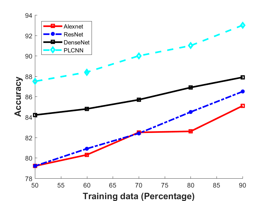
Influence of dataset size: To show that our model is robust and performs better, we start from a 90%:10% training:testing split and then reduce the training partition by 10% each time and increase the testing set by 10%. Figure 7 presents the performance of each model on HeLa dataset boland2001neural . The results of ResNet he2016deep and AlexNet krizhevsky2012imagenet are below 80% while our’s is the highest when the split is 60%. Meanwhile, if 90% dataset is reserved for training, then the testing part is 10%, and our method’s accuracy is 5.1% higher than the second-best performing DenseNet huang2017denseNet model. Overall, our method leads for all the training and testing partitions, which indicates our algorithm’s robust architecture.

Training size effect on traditional algorithms: Next, we investigate the training dataset’s effect on our model and classical algorithms. The performances of the classical algorithms on LOCATE and CHO datasets are very high. However, this could be due to the small amount of data reserved for testing, usually between 5% to 10%. We present the effect of decreasing training data size in Table 4, which illustrates the classical methods’ high results due to more training data as compared to test data. When training data decreases, the accuracy drops. Note that results are shown in Table 4 for traditional algorithms are the ensemble-based accuracies occluding our claim regarding performance drop. Detailed results for the individual members of the same ensemble are given in Table 5, where the effect of increasing test data is evident. Contrary to the traditional algorithms, our PLCNN performs consistently better on all three datasets, as the drop in performance is almost negligible.

Table 5: ETAS accuracies for individual members of ensemble on CHO dataset for $\tau$ = 40. Here, $\mu$ refers to the average intensity value of the image and $\tau$ indicates the threshold of the pixel intensities for calculating the average.

Feature Name 90%-10% 80%-20% 70%-30% 60%-40% $\mu$ to $255$ 93.2 92.6 92.0 91.4 $\mu$ to $255-\tau$ 30.5 28.7 27.2 26.9 $\mu+\tau$ to $255$ 91.4 90.5 90.2 89.2 $\mu+\tau$ to $255-\tau$ 29.3 28.4 27.5 26.2 $\mu-\tau$ to $255$ 91.4 89.9 89.2 89.2 $\mu-\tau$ to $255-\tau$ 29.6 29.6 26.6 26.2 $\mu-\tau$ to $\mu+\tau$ 32.1 31.8 31.4 30.8

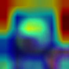
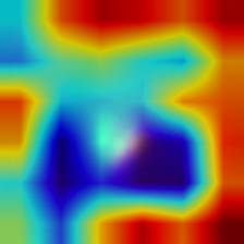
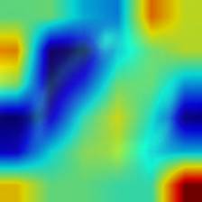
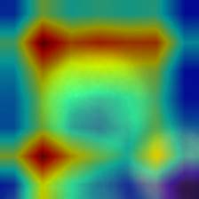
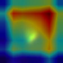
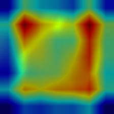
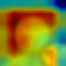
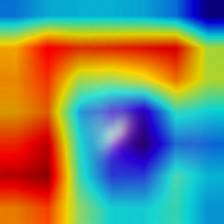
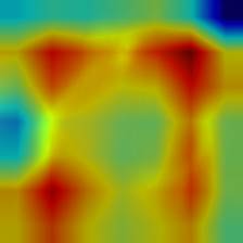
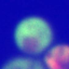
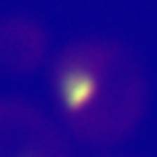
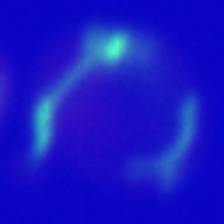
Image attentions: Attention mechanisms anwar2019densely ; anwar2019real are used in many computer vision applications to learn about the focus of networks. Though we have not explicitly applied our network’s attention, we illustrate here that our method focuses on the object of interest. We utilize Grad-CAM selvaraju2017grad to visualize the attention of the networks. The features before the last layer are collected and provided to the Grad-CAM selvaraju2017grad . Figure 8 illustrates the focus of each CNN method on sample images from CHO and Yeast datasets. Our method provides the best results due to the correct identification of proteins present in the images.

Figure 10: Confusion matrix for Yeast dataset. The predicted organelle are shown in the columns while the true values are present in the rows. The summaries of accuracies are given in the last row and column.

Confusion matrices: We present confusion matrix for CHO dataset boland1998automated in Figure 9 for the PLCNN, aggregating the results for all cross-validations. The correctly classified organelle classes are given along the matrix’s diagonal, while the non-diagonal elements show the misclassified organelles. Mostly, the non-diagonal elements are zeros. The overall accuracy is in the diagonal’s final element, while the individual accuracy is summarized in the right column and last row. Besides, the diagonal shows the accuracies contributed by each organelle. Our PLCNN perfectly classifies four out of the five organelle types. The only incorrect classification is for Golgi, where the accuracy is 97.7% as our PLCNN confuses one image of Golgi and Lysosome. These results are consistent with the traditional classifiers, and the incorrect classification may be due to the very similar patterns in these images.

Our results are better than the previous best-performing method i.e. M-CNN godinez2017multi ; for example, PLCNN accuracy on “Nucleolus” is 100% while the M-CNN godinez2017multi is only 81%. Moreover, our method is also superior in performance to M-CNN, which requires manual intervention.

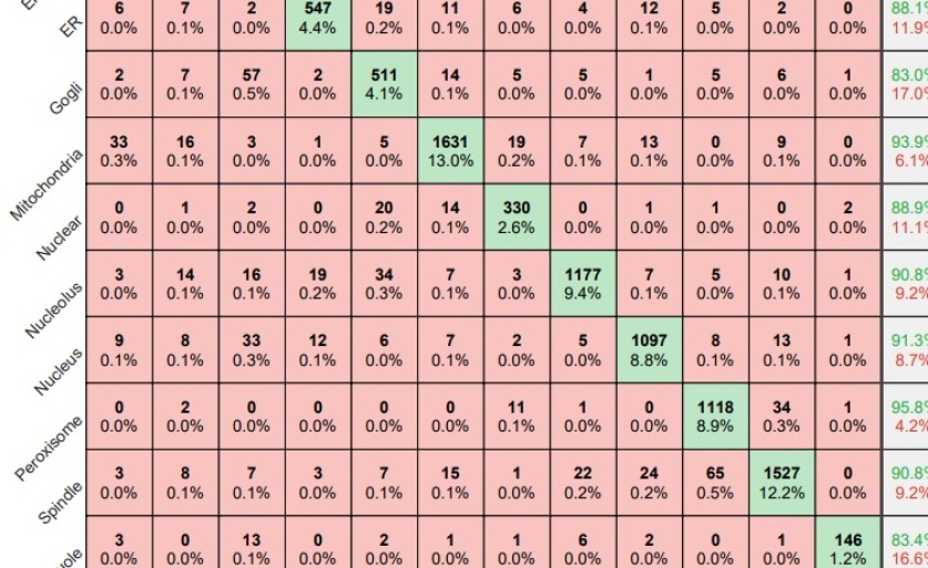
Figure 10 displays the confusion matrix computed for Yeast dataset parnamaa2017accurate . Again, the correctly classified elements are along the diagonal while the incorrect ones are along with the non-diagonal spaces. The precision is the last column in the given matrix, while the recall is the last row. The PLCNN performs relatively better on six protein types i.e. “Cell”, “Mitochondria”, “Nuclear”, “Nucleus”, “Peroxisome” and “Spindle” while for the remaining classes, the precision is more than 82%, this may be due to the low number of training images. The most confusion is between the protein types of “Cell” and “Cytoplasm”, which equates to be 0.4%. On the other hand, the low recall PLCNN reported is for “Gogli” protein, which is 74.2%; however, the recall for other types is more than 88%.

Prediction confidence: We compare the prediction confidence of traditional classifiers trained on Yeast and HeLa datasets against our PLCNN on four images as shown in Figure 11. Each image has the prediction probabilities for each algorithm underneath. The red color shows when the prediction is incorrect, whereas the green is for the correct outcome. It can be observed that our method predicts the correct labels with high confidence, while the probability is very low when the prediction is incorrect. The image in the first column in Figure 11 is very challenging due to minimum texture and almost no structure. All the methods failed to identify the type of protein in the mentioned image correctly. However, the competing methods prediction scores are much higher than ours. Similarly, our algorithm confidence is always high when the prediction is correct and low when it is incorrect. This shows the learning capability of our network.

AlexNet	0.32	0.57	0.79	0.82
ResNet	0.69	0.68	0.49	1
DenseNet	0.60	0.79	0.75	0.90
PLCNN	0.26	0.88	1	1

Figure 11: The correct predictions are highlighted via green while the red depicts incorrect. Our method prediction score is high for true outcome and vice versa.

5 Conclusion

Fluorescence microscopy techniques provide a powerful mechanism to obtain protein images from living cells. We have proposed an end-to-end PLCNN approach to analyze protein localization images from fluorescence microscopy images in this work. Our proposed approach can predict subcellular locations from protein images utilizing intensity values as input to the network. We have also tested some of the other CNN variations using benchmark protein image datasets. PLCNN consistently outperformed the existing state-of-the-art machine learning and deep learning models over a diverse set of protein localization datasets. Our approach computes the output probabilities of the network to predict the protein localization quantitatively.

The image attention analysis reveals that the PLCNN network can capture objects of interest in protein imagery while ignoring irrelevant and unnecessary details. Our proposed approach’s generalizing capability is validated from its consistent performance across all the utilized datasets over several images from different backgrounds. Comparative analysis reveals that our proposed approach is either better or comparable to the current state-of-the-art models. Particularly, the recognition capability of PLCNN on HeLa and Yeast images needs further improvement.

Experimental results reveal that pattern recognition-based procedures can be developed to simplify bioinformatics-based solutions to aid drug discovery in the pharmaceutical industry. Thus a critical aspect of our future work would be to develop a real-time state-of-the-art application that will be able to recognize protein images as soon as they are obtained from living cells. However, such development will require a more in-depth quantitative analysis of protein imagery.

6 Declarations

Funding

This research did not receive any specific funding.

Conflict of interest

The authors declare that they have no conflict of interest.

Ethics approval

Since no experiments are performed on humans or animals (dead or alive) in this research, therefore, Ethical approval is not required.

Availability of data and material

Publicly available datasets are used in this study.

Code availability

Code available at https://github.com/saeed-anwar/PLCNN

References

- (1) Yang, F., Xu, Y.Y., Wang, S.T., Shen, H.B.: Image-based classification of protein subcellular location patterns in human reproductive tissue by ensemble learning global and local features. Neurocomputing 131, 113–123 (2014)
- (2) Chong, Y.T., Koh, J.L., Friesen, H., Duffy, S.K., Cox, M.J., Moses, A., Moffat, J., Boone, C., Andrews, B.J.: Yeast proteome dynamics from single cell imaging and automated analysis. Cell 161(6), 1413–1424 (2015)
- (3) Pärnamaa, T., Parts, L.: Accurate classification of protein subcellular localization from high-throughput microscopy images using deep learning. G3: Genes, Genomes, Genetics 7(5), 1385–1392 (2017)
- (4) Shao, W., Ding, Y., Shen, H.B., Zhang, D.: Deep model-based feature extraction for predicting protein subcellular localizations from bio-images. Frontiers of Computer Science 11(2), 243–252 (2017)
- (5) Glory, E., Murphy, R.F.: Automated subcellular location determination and high-throughput microscopy. Developmental cell 12(1), 7–16 (2007)
- (6) Xu, Y.Y., Yao, L.X., Shen, H.B.: Bioimage-based protein subcellular location prediction: a comprehensive review. Frontiers of Computer Science 12(1), 26–39 (2018)
- (7) Tahir, M., Khan, A., Majid, A.: Protein subcellular localization of fluorescence imagery using spatial and transform domain features. Bioinformatics 28(1), 91–97 (2011)
- (8) Itzhak, D.N., Tyanova, S., Cox, J., Borner, G.H.: Global, quantitative and dynamic mapping of protein subcellular localization. Elife 5, e16950 (2016)
- (9) Xiang, S., Liang, Q., Hu, Y., Tang, P., Coppola, G., Zhang, D., Sun, W.: Amc-net: Asymmetric and multi-scale convolutional neural network for multi-label hpa classification. Computer Methods and Programs in Biomedicine 178, 275–287 (2019)
- (10) Kreft, M., Milisav, I., Potokar, M., Zorec, R.: Automated high through-put colocalization analysis of multichannel confocal images. Computer Methods and Programs in Biomedicine 74(1), 63–67 (2004)
- (11) Tahir, M., Khan, A.: Protein subcellular localization of fluorescence microscopy images: Employing new statistical and texton based image features and svm based ensemble classification. Information Sciences 345, 65–80 (2016)
- (12) Boland, M.V., Markey, M.K., Murphy, R.F.: Automated recognition of patterns characteristic of subcellular structures in fluorescence microscopy images. Cytometry: The Journal of the International Society for Analytical Cytology 33(3), 366–375 (1998)
- (13) Murphy, R.F., Boland, M.V., Velliste, M., et al.: Towards a systematics for protein subcellular location: Quantitative description of protein localization patterns and automated analysis of fluorescence microscope images. In: ISMB. pp. 251–259 (2000)
- (14) Huang, K., Murphy, R.F.: Boosting accuracy of automated classification of fluorescence microscope images for location proteomics. BMC Bioinformatics 5(1), 78 (2004)
- (15) Hamilton, N.A., Pantelic, R.S., Hanson, K., Teasdale, R.D.: Fast automated cell phenotype image classification. BMC Bioinformatics 8(1), 110 (2007)
- (16) Chebira, A., Barbotin, Y., Jackson, C., Merryman, T., Srinivasa, G., Murphy, R.F., Kovačević, J.: A multiresolution approach to automated classification of protein subcellular location images. BMC Bioinformatics 8(1), 210 (2007)
- (17) Nanni, L., Lumini, A.: A reliable method for cell phenotype image classification. Artificial intelligence in medicine 43(2), 87–97 (2008)
- (18) Nanni, L., Lumini, A., Brahnam, S.: Local binary patterns variants as texture descriptors for medical image analysis. Artificial intelligence in medicine 49(2), 117–125 (2010)
- (19) Li, C., Wang, X.h., Zheng, L., Huang, J.f.: Automated protein subcellular localization based on local invariant features. The protein journal 32(3), 230–237 (2013)
- (20) Zhang, B., Pham, T.D.: Phenotype recognition with combined features and random subspace classifier ensemble. BMC Bioinformatics 12(1), 128 (2011)
- (21) Tahir, M., Jan, B., Hayat, M., Shah, S.U., Amin, M.: Efficient computational model for classification of protein localization images using extended threshold adjacency statistics and support vector machines. Computer methods and programs in biomedicine 157, 205–215 (2018)
- (22) Nanni, L., Ghidoni, S., Brahnam, S.: Handcrafted vs. non-handcrafted features for computer vision classification. Pattern Recognition 71, 158–172 (2017)
- (23) Xiao, M., Shen, X., Pan, W.: Application of deep convolutional neural networks in classification of protein subcellular localization with microscopy images. Genetic epidemiology 43(3), 330–341 (2019)
- (24) Kraus, O.Z., Grys, B.T., Ba, J., Chong, Y., Frey, B.J., Boone, C., Andrews, B.J.: Automated analysis of high-content microscopy data with deep learning. Molecular systems biology 13(4), 924 (2017)
- (25) Le, N.Q.K., Huynh, T.T., Yapp, E.K.Y., Yeh, H.Y.: Identification of clathrin proteins by incorporating hyperparameter optimization in deep learning and pssm profiles. Computer Methods and Programs in Biomedicine 177, 81–88 (2019)
- (26) Zhang, L., Yu, G., Xia, D., Wang, J.: Protein–protein interactions prediction based on ensemble deep neural networks. Neurocomputing 324, 10–19 (2019)
- (27) Guo, Y., Shang, X., Li, Z.: Identification of cancer subtypes by integrating multiple types of transcriptomics data with deep learning in breast cancer. Neurocomputing 324, 20–30 (2019)
- (28) Gu, J., Wang, Z., Kuen, J., Ma, L., Shahroudy, A., Shuai, B., Liu, T., Wang, X., Wang, G., Cai, J., et al.: Recent advances in convolutional neural networks. Pattern Recognition 77, 354–377 (2018)
- (29) Dürr, O., Sick, B.: Single-cell phenotype classification using deep convolutional neural networks. Journal of biomolecular screening 21(9), 998–1003 (2016)
- (30) Krizhevsky, A., Sutskever, I., Hinton, G.E.: Imagenet classification with deep convolutional neural networks. In: Advances in Neural Information Processing Systems. pp. 1097–1105 (2012)
- (31) Tibshirani, R.: Regression shrinkage and selection via the lasso. Journal of the Royal Statistical Society. Series B (Methodological) 58(1), 267–288 (1996)
- (32) Godinez, W.J., Hossain, I., Lazic, S.E., Davies, J.W., Zhang, X.: A multi-scale convolutional neural network for phenotyping high-content cellular images. Bioinformatics 33(13), 2010–2019 (2017)
- (33) Simonyan, K., Zisserman, A.: Very deep convolutional networks for large-scale image recognition. In: Proceedings of the International Conference on Learning Representations (2015)
- (34) He, K., Zhang, X., Ren, S., Sun, J.: Deep residual learning for image recognition. In: Proceedings of the IEEE conference on computer vision and pattern recognition. pp. 770–778 (2016)
- (35) Szegedy, C., Ioffe, S., Vanhoucke, V., Alemi, A.A.: Inception-v4, inception-resnet and the impact of residual connections on learning. In: AAAI. vol. 4, p. 12 (2017)
- (36) Sabour, S., Frosst, N., Hinton, G.E.: Dynamic routing between capsules. In: NIPS. pp. 3856–3866 (2017)
- (37) Lao, Q., Fevens, T.: Cell phenotype classification using deep residual network and its variants. International Journal of Pattern Recognition and Artificial Intelligence 33(11), 1940017 (2019)
- (38) Zagoruyko, S., Komodakis, N.: Wide residual networks. In: Proceedings of the British Machine Vision Conference (BMVC). pp. 1–12. BMVA Press (September 2016)
- (39) Xie, S., Girshick, R., Dollár, P., Tu, Z., He, K.: Aggregated residual transformations for deep neural networks. In: CVPR. pp. 5987–5995. IEEE (2017)
- (40) Han, D., Kim, J., Kim, J.: Deep pyramidal residual networks. In: CVPR. pp. 6307–6315. IEEE (2017)
- (41) Huang, G., Liu, Z., Van Der Maaten, L., Weinberger, K.Q.: Densely connected convolutional networks. In: Proceedings of the IEEE Conference on Computer Vision and Pattern Recognition. pp. 4700–4708 (2016)
- (42) Anwar, S., Barnes, N.: Densely residual laplacian super-resolution. IEEE Transactions on Pattern Analysis and Machine Intelligence (2020)
- (43) Boland, M.V., Murphy, R.F.: A neural network classifier capable of recognizing the patterns of all major subcellular structures in fluorescence microscope images of hela cells. Bioinformatics 17(12), 1213–1223 (2001)
- (44) Szegedy, C., Liu, W., Jia, Y., Sermanet, P., Reed, S., Anguelov, D., Erhan, D., Vanhoucke, V., Rabinovich, A.: Going deeper with convolutions. In: CVPR. pp. 1–9 (2015)
- (45) Ruder, S.: An overview of gradient descent optimization algorithms. arXiv preprint arXiv:1609.04747 (2016)
- (46) Ljosa, V., Sokolnicki, K.L., Carpenter, A.E.: Annotated high-throughput microscopy image sets for validation. Nature methods 9(7), 637–637 (2012)
- (47) Selvaraju, R.R., Cogswell, M., Das, A., Vedantam, R., Parikh, D., Batra, D.: Grad-cam: Visual explanations from deep networks via gradient-based localization. In: ICCV. pp. 618–626 (2017)
- (48) Nanni, L., Brahnam, S., Alessandra, L.: Selecting the best performing rotation invariant patterns in local binary/ternary patterns. In: International conference on IP, computer vision, and pattern recognition. pp. 369–375 (2010)
- (49) Lin, C.C., Tsai, Y.S., Lin, Y.S., Chiu, T.Y., Hsiung, C.C., Lee, M.I., Simpson, J.C., Hsu, C.N.: Boosting multiclass learning with repeating codes and weak detectors for protein subcellular localization. Bioinformatics 23(24), 3374–3381 (2007)
- (50) Nanni, L., Brahnam, S., Ghidoni, S., Lumini, A.: Bioimage classification with handcrafted and learned features. IEEE/ACM transactions on computational biology and bioinformatics 16(3), 874–885 (2018)
- (51) Nanni, L., Brahnam, S., Ghidoni, S., Maguolo, G.: General purpose (genp) bioimage ensemble of handcrafted and learned features with data augmentation. arXiv preprint arXiv:1904.08084 (2019)
- (52) Anwar, S., Barnes, N.: Real image denoising with feature attention. In: ICCV (October 2019)