Discovery of a Photoionized Bipolar Outflow towards the Massive Protostar G45.47+0.05

Abstract

Massive protostars generate strong radiation feedback, which may help set the mass they achieve by the end of the accretion process. Studying such feedback is therefore crucial for understanding the formation of massive stars. We report the discovery of a photoionized bipolar outflow towards the massive protostar G45.47+0.05 using high-resolution observations at 1.3 mm with the Atacama Large Millimeter/Submillimeter Array (ALMA) and at 7 mm with the Karl G. Jansky Very Large Array (VLA). By modeling the free-free continuum, the ionized outflow is found to be a photoevaporation flow with an electron temperature of $10,000~{}{\rm K}$ and an electron number density of $\sim 1.5\times 10^{7}~{}\mathrm{cm}^{-3}$ at the center, launched from a disk of radius of $110~{}\mbox{au}$. H30$\alpha$ hydrogen recombination line emission shows strong maser amplification, with G45 being one of very few sources to show such millimeter recombination line masers. The mass of the driving source is estimated to be $30-50~{}M_{\odot}$ based on the derived ionizing photon rate, or $30-40~{}M_{\odot}$ based on the H30$\alpha$ kinematics. The kinematics of the photoevaporated material is dominated by rotation close to the disk plane, while accelerated to outflowing motion above the disk plane. The mass loss rate of the photoevaporation outflow is estimated to be $\sim(2-3.5)\times 10^{-5}~{}M_{\odot}~{}{\rm yr}^{-1}$. We also found hints of a possible jet embedded inside the wide-angle ionized outflow with non-thermal emissions. The possible co-existence of a jet and a massive photoevaporation outflow suggests that, in spite of the strong photoionization feedback, accretion is still on-going.

1 Introduction

Massive stars dominate the radiative, mechanical and chemical feedback to the interstellar medium, thus regulating the evolution of galaxies. However, their formation process is not well understood. One key difference between high- and low-mass star formation is that massive protostars become so luminous that they generate strong radiation feedback, which potentially stops the accretion. For example, radiation pressure was considered a potential barrier for massive star formation (Wolfire & Cassinelli, 1987; Yorke & Sonnhalter, 2002). Photoionization is another important feedback process, as massive protostars emit large amounts of Lyman continuum photons that ionize the accretion flows to form photoevaporative outflows driven by the thermal pressure of $\sim 10^{4}~{}{\rm K}$ ionized gas (Hollenbach et al., 1994). However, theoretical calculations and simulations have suggested that, in the core accretion scenario these feedback processes are not strong enough to stop accretion (Krumholz et al., 2009; Kuiper et al., 2010; Peters et al., 2010; Tanaka & Nakamoto, 2011). Tanaka et al. (2017) studied the combined effects from various feedback processes in massive star formation, including magnetohydrodynamical (MHD) disk winds, radiation pressure, photoionization and stellar winds, finding that MHD winds are dominant, while the others processes play relatively minor roles. However, observational confirmation of such a theoretical scenario is still difficult, due to the rarity and typically large distances of massive protostars, especially the most massive type with strong radiation feedbacks.

The protostar G45.47+0.05 (hereafter G45; $d=8.4~{}\mbox{kpc}$, Wu et al. 2019) has a luminosity of $\sim(2-5)\times 10^{5}~{}L_{\odot}$ and a mass of $\sim 20-50~{}M_{\odot}$ (De Buizer et al. 2017), based on infrared spectral energy distribution (SED) fitting (Zhang & Tan 2018). G45 is associated with an ultracompact (UC) H ii region (Wood & Churchwell 1989; Urquhart et al. 2009; Rosero et al. 2019) and OH and H₂O masers (Forster & Caswell 1989). Molecular outflows are seen in HCO⁺($1-0$), with blue-shifted emission to the north and red-shifted emission to the south, consistent with the elongation of radio continuum emission (Wilner et al. 1996). Infrared observations at $10-40~{}\mu$m show extended emission offset to the north of the UCH ii region (De Buizer et al. 2005, 2017), which may come from the near-facing (blue-shifted) outflow cavity. The offset between the infrared emission and the UCH ii region may be due to the high infrared extinction towards the protostar, suggesting dense molecular gas surrounds the source.

2 Observations

ALMA 1.3 mm observations were performed on 2016 April 24, 2016 September 4 and 2017 November 2 with C36-3, C36-6 and C43-9 configurations (hereafter C3, C6 and C9), with on-source integration times of 3.6, 7.3 and 17.7 min, respectively (project IDs: 2015.1.01454.S; 2017.1.00181.S). J1751+0939, J2025+3343 and J2000-1748 were used for bandpass calibration; Titan, J2148+0657 and J2000-1748 were used for flux calibration; and J1922+1530, J1914+1636 and J1922+1530 were used as phase calibrators. The data were calibrated and imaged in CASA (McMullin et al. 2007). Self-calibration was performed for the three configuration data separately using the continuum data (bandwidth of 2 GHz), and applied to the line data. Images are made with the CASA task tclean using robust weighting (Briggs 1995) with the robust parameter of 0.5. The synthesized beam sizes of different configurations are listed in Figure 1. Here we focus on continuum and H30$\alpha$ line (231.90093 GHz) data, deferring analysis of molecular lines to a future paper.

The VLA 7 mm observation was performed in 2014 with A configuration and two 4-GHz basebands centered at 41.9 and 45.9 GHz (project ID: 14A-113). Details of the VLA data is summarized by Rosero et al. (2019).

3 Results

3.1 1.3 and 7 mm continuum

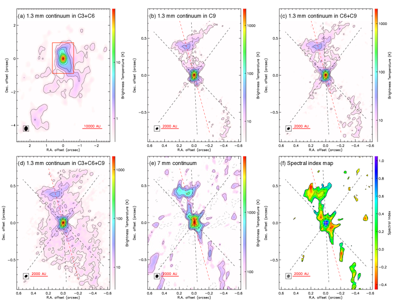
Figure 1: (a)$-$(d): ALMA 1.3 mm continuum map of G45 observed in the C3+C6 configuration (panel a), C9 configuration (panel b), C6+C9 configuration (panel c), and C3+C6+C9 configuration (panel d). The synthesized beams in these images are $0.28^{\prime\prime}\times 0.21^{\prime\prime}$ ($\mathrm{P.A.}=-6.6^{\circ}$, panel a), $0.038^{\prime\prime}\times 0.026^{\prime\prime}$ ($\mathrm{P.A.}=-53.9^{\circ}$, panel b), $0.042^{\prime\prime}\times 0.028^{\prime\prime}$ ($\mathrm{P.A.}=-53.6^{\circ}$, panel c), and $0.043^{\prime\prime}\times 0.029^{\prime\prime}$ ($\mathrm{P.A.}=-53.4^{\circ}$, panel d). The contour levels are $5\sigma\times 2^{n}$ ($n=0,1,...$), with $1\sigma=0.13~{}{\rm K}$ ($0.33~{}\mbox{mJy}~{}\mbox{beam}^{-1}$, panel a), $1\sigma=1.1~{}{\rm K}$ ($0.049~{}\mbox{mJy}~{}\mbox{beam}^{-1}$, panel b), $1\sigma=0.91~{}{\rm K}$ ($0.047~{}\mbox{mJy}~{}\mbox{beam}^{-1}$, panel c), and $1\sigma=0.94~{}{\rm K}$ ($0.052~{}\mbox{mJy}~{}\mbox{beam}^{-1}$, panel d). (e): VLA 7 mm continuum map with solid contours at $5\sigma\times 2^{n}$ ($n=0,1,...,6$, $1\sigma=25~{}{\rm K}$ or $0.067~{}\mbox{mJy}~{}\mbox{beam}^{-1}$), and dashed contours at $-5\sigma$ and $-10\sigma$. The synthesized beam is $0.045^{\prime\prime}\times 0.038^{\prime\prime}$ with $\mathrm{P.A.}=-24.2^{\circ}$. (f): Map of continuum spectral index between 1.3 mm (C3+C6+C9) and 7 mm, $\alpha_{\nu}=\log(I_{\nu_{1}}/I_{\nu_{2}})/\log(\nu_{1}/\nu_{2})$, where $\nu_{1}=44~{}\mbox{GHz}$ and $\nu_{2}=234~{}\mbox{GHz}$. Only regions where both 1.3 and 7 mm emissions are $>5\sigma$ are included. Here the 1.3 mm image is restored with the same beam size as the 7 mm image. The red rectangle in panel a marks the region shown in panels b$-$f. In panels b$-$f, the black dashed lines indicate the outflow axis ($\mathrm{P.A.}=3^{\circ}$) and projected half-opening angle ($40^{\circ}$), and the red dashed line indicates a possible jet ($\mathrm{P.A.}=15^{\circ}$). The R.A. and Dec. offsets in all the panels are relative to the continuum peak position from the ALMA C9 configuration data, $(\alpha_{2000},\delta_{2000})=(19^{\mathrm{h}}14^{\mathrm{m}}25^{\mathrm{s}}.678$, $+11^{\circ}09\arcmin 25\arcsec.567)$.

The 1.3 mm continuum emission appears concentrated within $5\arcsec$ ($4.2\times 10^{4}\>\mbox{au}$) from the central source (Figure 1a). At low resolution (C3+C6 configuration), the continuum emission is elongated in the north-south direction, with extended structures towards the south. At high resolution (C9 configuration), the continuum shows an hourglass shape aligned in the north-south direction (Figure 1b), with a morphology highly symmetric with respect to an axis with $\mathrm{P.A.}\approx 3^{\circ}$, which is consistent with the direction of the HCO⁺ outflow (§1). The apparent half-opening angle of this hourglass is $\sim 40^{\circ}$ (dashed lines in Figure 1b). More extended emissions are recovered by combining with more compact configuration data (panels c and d). The bipolarity can be still clearly seen in the combined images, and most of the fainter extended emissions are inside of the outflow cavity to the north and south. The 7 mm continuum (panel e) has very similar morphology as the high-resolution 1.3 mm continuum. At both 1.3 and 7 mm, most of the compact continuum emissions are concentrated within $0.2\arcsec$ ($1.7\times 10^{3}~{}\mbox{au}$) from the central source. Another emission peak is seen $\sim 0.4\arcsec$ to the north, which was first identified by Rosero et al. (2019). Its emission appears to be more extended and shows an arc-like shape facing away from the main source in a direction consistent with the main outflow, suggesting that the northern emission structure is part of the main outflow.

Figure 1f shows the spectral index map derived using the 1.3 and 7 mm continuum intensities, $\alpha_{\nu}=\log(I_{\nu_{1}}/I_{\nu_{2}})/\log(\nu_{1}/\nu_{2})$, where $\nu_{1}=44$ GHz and $\nu_{2}=234$ GHz. Note that the position of the 1.3 mm emission peak is slightly offset from either the emission peak or the center of symmetry of the 7 mm image (see Figure 1e). Therefore, we manually shift the 7 mm image by 7 mas in the R.A. direction and 13 mas in the Dec. direction, so that the 1.3 mm emission peak coincides with the 7 mm center of symmetry in making the spectral index map (also see Figure 3d). The central region has spectral indices of $\alpha_{\nu}>0.5$, indicating partially optically thick ionized gas ($\alpha_{\nu}=2$ for completely optically thick free-free emission), while more extended structures have spectral indices of $\alpha_{\nu}\approx 0$, consistent with optically thin free-free emission (e.g., Anglada et al. 2018). Note that, for dust continuum emission, the index is $\alpha_{\nu,\mathrm{dust}}=2$ in the optically thick case and $3\lesssim\alpha_{\nu,\mathrm{dust}}\lesssim 4$ in the optically thin case (assuming a typical dust emissivity spectral index of $1-2$). These suggest that in this source, even at 1.3 mm, the compact continuum emission may have a significant free-free contribution, if not dominated by it. This is further supported by the fact that the 1.3 and 7 mm continuum emissions coincide well with the H30$\alpha$ hydrogen recombination line (HRL) emission (Figure 2a; see below). Furthermore, the 1.3 mm peak brightness temperature is $\sim 2000~{}{\rm K}$, higher than that expected from dust continuum (the average dust temperature within 1000 au from a $\sim 30\>M_{\odot}$ protostar is estimated to be several $\times 10^{2}\>{\rm K}$ from dust continuum radiative transfer (RT) simulations by Zhang & Tan (2018)) and the dust sublimation temperature ($\sim 1600~{}{\rm K}$), but can be naturally explained by thermal emission from ionized gas with a typical temperature of $10^{4}\>{\rm K}$ around massive protostars.

However, the extended 1.3 mm continuum emission shown in the low-resolution data should still be dominated by dust emission. The total 1.3 mm continuum flux $>3\sigma$ within $5\arcsec$ from the central source measured from the C3+C6 image is 0.77 Jy. The compact structure within $0.9\arcsec$ has a total $>3\sigma$ flux of 0.34 Jy measured from the C9 image, or 0.61 Jy from the C3+C6+C9 image, which can be considered as an estimate (upper limit) of the free-free flux. Their difference of 0.16 to 0.43 Jy can be used as an estimate (lower limit) for the extended dust continuum flux of the source, which corresponds to a gas mass of $(2.1-5.6)\times 10^{2}\>M_{\odot}$ assuming a temperature of 30 K (typically assumed for molecular cores), or $(0.95-2.6)\times 10^{2}~{}M_{\odot}$ assuming 60 K (suitable for within $\sim 10,000~{}\mbox{au}$ around a $20-50~{}M_{\odot}$ protostar; Zhang & Tan 2018). Here we adopt a dust opacity of $\kappa_{\mathrm{1.3mm}}=0.899~{}\mathrm{cm}^{2}~{}\mathrm{g}^{-1}$ (Ossenkopf & Henning 1994) and a gas-to-dust mass ratio of 141 (Draine 2011). These mass estimates suggest that there is a large mass reservoir for future growth of the massive protostar.

Inside the wide-angle hourglass outflow cavity, a narrower jet-like feature is apparent in the 1.3 mm images with $\mathrm{P.A.}\approx 15^{\circ}$ (red dashed line in Figure 1). Along this direction, a structure separate from the outflow cavity walls extends from the central source to the northern lobe. To the south, along the same direction, there is an additional emission peak $\sim 0.1\arcsec$ from the center, and also a stream of extended emission. These are most clearly seen in Figures 1b and 1c. Along this direction, there are also some emission features in the 7 mm image. However, some of these may arise from strong side-lobe patterns from incomplete uv sampling in the VLA observation. As shown in Figure 1f, some regions have negative spectral indices of $-0.5<\alpha_{\nu}<-0.2$, inconsistent with pure free-free emission or dust emission, indicating possible contributions from nonthermal synchrotron emission, which is occasionally found associated with massive protostellar jets (e.g., Garay et al. 1996; Carrasco-González et al. 2010; Moscadelli et al. 2013; Rosero et al. 2016; Beltrán et al. 2016; Sanna et al. 2019). Thus, detection of negative spectral indices is also consistent with a jet being embedded inside the wide-angle ionized outflow. Evidence for the coexistence of wide-angle outflows with collimated jets has been found in other massive young stellar sources, such as Cepheus A HW2, where water masers trace a wide outflow and free-free continuum traces a collimated jet (Torrelles et al. 2011).

3.2 H30$\alpha$ line

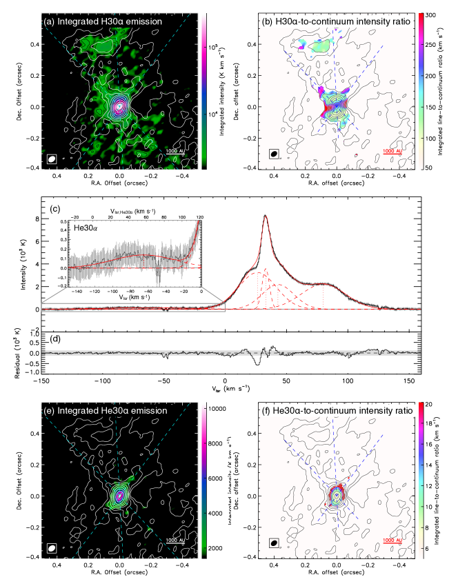
Figure 2: (a): H30$\alpha$ emission map observed in ALMA C3+C6+C9 configuration, integrated in the velocity range $-10<V_{\mathrm{lsr}}<+130~{}\mbox{km s}^{-1}$ (color scale and black contours at $5\sigma\times 2^{n}$, $n=1,2,3,...$, $1\sigma=500~{}{\rm K}~{}\mbox{km s}^{-1}$ or $0.036~{}\mbox{Jy}~{}\mbox{beam}^{-1}~{}\mbox{km s}^{-1}$), overlaid with the 1.3 mm continuum in white contours. The dashed lines in panels indicate the outflow axis ($\mathrm{P.A.}=3^{\circ}$) and projected opening angle ($40^{\circ}$). (b): Map of the integrated H30$\alpha$ line-to-continuum ratio ($\int_{v}I_{\mathrm{H30}\alpha}dv/I_{\mathrm{1.3~{}mm}}$, color scale), overlaid with the continuum (black contours). (c): H30$\alpha$ and He30$\alpha$ spectra (solid black line) at the continuum peak position. The $3\sigma$ noise is marked by the error bar in each velocity channel. The red solid curve is the fitted profile combining multiple Gaussian components, each of which is shown by the dashed curves with their central velocities indicated by the dotted lines. The inset panel shows a zoom-in view of the He30$\alpha$ spectrum. (d): The residual between the observed spectrum and the fitted profile. The shaded region indicates the 3$\sigma$ noise level. (e): Same as panel a, but showing the He30$\alpha$ emission integrated in the velocity range $-150<V_{\mathrm{lsr,H30}\alpha}<-20~{}\mbox{km s}^{-1}$ ($-28<V_{\mathrm{lsr,He30}\alpha}<+102~{}\mbox{km s}^{-1}$). The black contours are at levels of $5\sigma\times 2^{n}$, $n=1,2,3,...$, $1\sigma=460~{}{\rm K}~{}\mbox{km s}^{-1}$ or $0.033~{}\mbox{Jy}~{}\mbox{beam}^{-1}~{}\mbox{km s}^{-1}$). (f): Same as panel d, but showing the integrated He30$\alpha$ line-to-continuum ratio ($\int_{v}I_{\mathrm{He30}\alpha}dv/I_{\mathrm{1.3~{}mm}}$).

The position and morphology of the H30$\alpha$ emission are found to coincide very well with the 1.3 and 7 mm continuum emissions (Figures 2a and 2b). Figure 2c shows the H30$\alpha$ spectrum at the 1.3 mm continuum peak. The H30$\alpha$ line has a complicated spectral profile, suggesting strong non-LTE effects and multiple dynamical components. In addition to the strong narrow feature at $V_{\mathrm{lsr}}=+33~{}\mbox{km s}^{-1}$ ($\mathrm{FWHM}=7~{}\mbox{km s}^{-1}$), the rest of the line profile can be relatively well fit with three Gaussian components at $V_{\mathrm{lsr}}=+25$, $+44$ and $+80~{}\mbox{km s}^{-1}$ with $\mathrm{FWHM}=36$, 42, and $30~{}\mbox{km s}^{-1}$ (the source systemic velocity is $V_{\mathrm{sys}}\sim+60~{}\mbox{km s}^{-1}$; Ortega et al. 2012).

To quantify the level of non-LTE emission, in Figure 2b we show the map of the integrated line-to-continuum (ILTC) intensity ratio, $\int_{v}I_{\mathrm{H30}\alpha}dv/I_{\mathrm{1.3~{}mm}}$, where $I_{\mathrm{H30}\alpha}$ is the H30$\alpha$ intensity and $I_{\mathrm{1.3~{}mm}}$ is the 1.3 mm continuum intensity. Under LTE conditions and assuming both optically thin free-free and H30$\alpha$ emissions, the ILTC intensity ratio is (see, e.g., eqs. 10.35, 14.27 and 14.29 of Wilson et al. 2013)

$$\frac{\int_{v}I_{\mathrm{H30}\alpha}dv}{I_{\mathrm{1.3~{}mm}}}=4.678\times 10^{6}~{}\mbox{km s}^{-1}\left(\frac{T_{\mathrm{e}}}{{\rm K}}\right)^{-1}$$

$$\times\left[1.5\ln\left(\frac{T_{\mathrm{e}}}{{\rm K}}\right)-8.443\right]^{-1}\left[1+\frac{N\left(\mathrm{He}^{+}\right)}{N\left(\mathrm{H}^{+}\right)}\right]^{-1}.$$ (1)

The last term results from electrons from He⁺ contributing to free-free emission but not to the HRL, and typically $N\left(\mathrm{He}^{+}\right)/N\left(\mathrm{H}^{+}\right)=0.08$. Assuming a characteristic ionized gas temperature of $T_{\mathrm{e}}=10^{4}\>{\rm K}$, $\int_{v}I_{\mathrm{H30}\alpha}dv/I_{\mathrm{1.3~{}mm}}=81\>\mbox{km s}^{-1}$, which is a reference value for the optically-thin LTE conditions. As Figure 2b shows, most of the H30$\alpha$ emission is stronger than expected under LTE conditions. In some parts, the measured ILTC ratio is $>200~{}\mbox{km s}^{-1}$ and reaching $\sim 300~{}\mbox{km s}^{-1}$, significantly higher than the LTE value of $81~{}\mbox{km s}^{-1}$, indicating strong maser amplification. Previously, millimeter HRL masers were detected in MWC349A, with an H30$\alpha$ ILTC ratio of $298\>\mbox{km s}^{-1}$ (Martín-Pintado et al. 1989; Jiménez-Serra et al. 2013), and also in H26$\alpha$ (weakly in H30$\alpha$) in MonR2-IRS2 (Jiménez-Serra et al. 2013). To our knowledge, G45 is only the third massive young stellar object to show strong millimeter HRL masers, with these reaching a similar level as in MWC349A. Figure 2b also shows that the strong maser effect is concentrated toward the east and west of the central source along a direction nearly perpendicular to the outflow axis, i.e., along the disk plane. This behavior is similar to that seen in MWC349A, in which HRL masers are found to be along certain annuli of the disk (e.g., Báez-Rubio et al. 2013; Zhang et al. 2017). In addition, there are two small regions along the outflow cavity walls to the north-east and north-west which also have strong maser levels.

Note that here we have assumed all the compact 1.3 mm continuum is free-free emission, which is reasonably valid, as discussed above. However, if there is a significant dust contribution in the 1.3 mm continuum, the observed ILTC ratio is then underestimated. Furthermore, if the H30$\alpha$ emission is not completely optically thin, the expected ILTC ratio under LTE conditions should be lower than the reference value of $81~{}\mbox{km s}^{-1}$. Both of these effects would imply even higher levels of maser amplification. In addition, the ionized gas temperature can also affect the LTE value of ILTC ratio, which ranges from $34~{}\mbox{km s}^{-1}$ with $T_{\mathrm{e}}=2\times 10^{4}~{}{\rm K}$ to $156~{}\mbox{km s}^{-1}$ with $T_{\mathrm{e}}=6\times 10^{3}~{}{\rm K}$. Even at the low temperature end of this range, maser amplification is needed to explain the observed ILTC ratios.

In addition to the H30$\alpha$ line, the He30$\alpha$ Helium recombination line (231.99543 GHz) is also detected (Figure 2c). Its spectrum can be fit with a single Gaussian profile at $V_{\mathrm{lsr,H30}\alpha}=-65~{}\mbox{km s}^{-1}$ ($V_{\mathrm{lsr,He30}\alpha}=+57~{}\mbox{km s}^{-1}$) and $\mathrm{FWHM}=83~{}\mbox{km s}^{-1}$. This line width is consistent with the total H30$\alpha$ line width. He30$\alpha$ integrated emission and ILTC ratio maps are shown in Figures 2e and 2f. The He30$\alpha$ ILTC ratio increases from $\sim 5~{}\mbox{km s}^{-1}$ at the center to $\sim 20~{}\mbox{km s}^{-1}$ in the outer region. The increasing ILTC ratio towards outside is unexpected, as the outer region should have lower ratio between Helium and Hydrogen ionizing photon rates. One possible explanation is that, the He30$\alpha$ emission also has maser effects with a similar level to H30$\alpha$ (the expected He30$\alpha$ ILTC ratio in optically thin LTE conditions is $6~{}\mbox{km s}^{-1}$ using similar formula as Eq. 1 and $T_{e}=10^{4}~{}{\rm K}$; note that He⁺⁺ is not considered), but at the center, the emission becomes partially optically thick, and the observed ILTC ratio decreases. Note that at $V_{\mathrm{lsr,H30}\alpha}\approx-50~{}\mbox{km s}^{-1}$, the dips are due to the absorption of CH₃OCHO $20_{9,12}-20_{8,13}$ line (231.9854 GHz) and CH₃OCH₃ $13_{0,13}-12_{1,12}$ line (231.9879 GHz) from the cooler surrounding material in the foreground.

4 Discussions

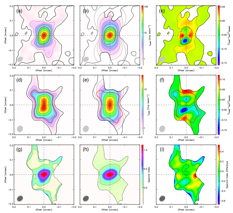
Figure 3: Comparisons between the model and observations in 1.3 mm continuum, 7 mm continuum and spectral index. (a): Observed 1.3 mm continuum map. (b): 1.3 mm continuum map from the best-fit model. (c): Differences between the observation and model $(I_{\mathrm{obs}}-I_{\mathrm{mod}})/I_{\mathrm{obs,peak}}$. (d)$-$(f): Same as panels a$-$c, but for the 7 mm continuum. (g)$-$(i): Same as panels a$-$c, but for the spectral index map. Only the regions with observed emissions $>10\sigma$ are shown. The red contours in panels a$-$f show the region with observed intensities $>0.1I_{\mathrm{obs,center}}$, which is used in the 2D model fitting. The maps are rotated by $3^{\circ}$ so that the outflow axis is along the $y$-axis. The 7 mm observational image is shifted by offsets of 7 mas in R.A. and 13 mas in Dec. to maximize the symmetry of the intensity profiles with respect to the center.

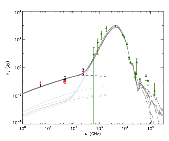
Figure 4: Observed SED of G45 compared to models. Green symbols and error bars show the fluxes from near-infrared to sub-mm wavelengths (De Buizer et al. 2017). Squares and error bars show the fluxes at 5, 42 and 46 GHz observed by VLA (Rosero et al. 2019). The red and black squares show the VLA fluxes integrated within $0.3\arcsec$ and $14\arcsec$ from the center, respectively. Triangles and error bars show the fluxes at ALMA Band 6 with assumed 10% error. The black triangle shows the ALMA flux observed in C3+C6 configuration and integrated within $5\arcsec$ from the center. The red and blue triangles show the ALMA fluxes within $0.9\arcsec$ from the center, observed in C3+C6+C9 and C9 configurations, respectively. The solid lines show the combined SEDs from free-free models and dust continuum models, and the dashed lines show the free-free model SEDs. The light dashed lines show the free-free SED from the model presented in Rosero et al. (2019), based on the photoionized MHD disk wind model by Tanaka et al. (2016). The dark dashed lines shows the free-free SEDs from the model presented in this work integrated over a region within $20000~{}\mbox{au}$ (2.4$\arcsec$) from the center. Best-fit models for different opening angles ($\theta_{w}$) are shown but the differences are small. The dust continuum models are from SED fitting by De Buizer et al. (2017) using the dust continuum radiative transfer model grid by Zhang & Tan (2018).

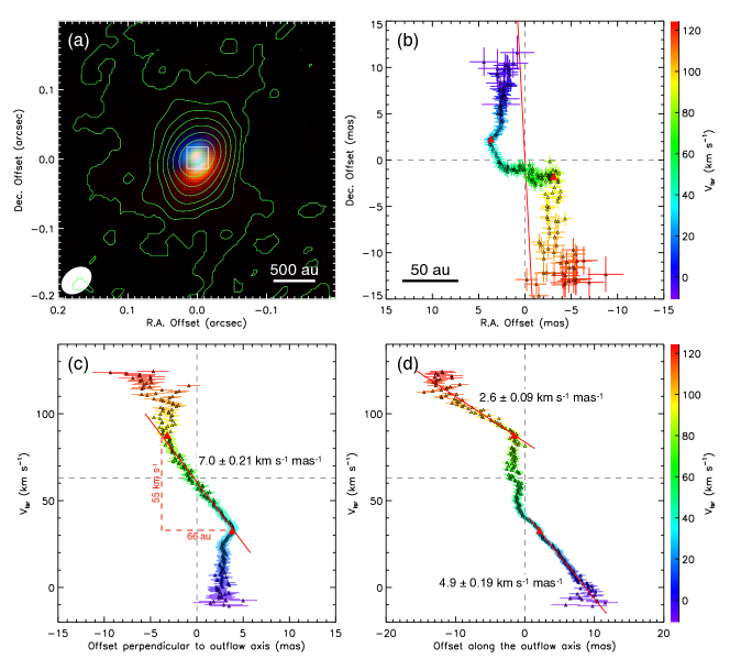
Figure 5: (a): Integrated blueshifted ($-10<V_{\mathrm{lsr}}<30~{}\mbox{km s}^{-1}$; blue color scale) and redshifted ($90<V_{\mathrm{lsr}}<130~{}\mbox{km s}^{-1}$; red color scale) H30$\alpha$ emissions, overlaid with total integrated emission ($-10<V_{\mathrm{lsr}}<130~{}\mbox{km s}^{-1}$; green contours; same as Figure 2a). The white square marks the region shown in panel b. (b): Distribution of the H30$\alpha$ emission centroids (triangles with error bars). Only channels with peak intensities $>10\sigma$ ($1\sigma=1.8~{}\mbox{mJy}~{}\mbox{beam}^{-1}$) are included. The position offsets are relative to the continuum peak. The line-of-sight velocities are shown by the color scale. The red line indicates the outflow axis ($\mathrm{P.A.}=3^{\circ}$). The large red triangles mark the positions where the centroid distribution pattern changes. (c): Distances of centroids from the continuum peak projected in the direction perpendicular to the outflow axis with their line-of-sight velocities. The red line indicates the fitted velocity gradient perpendicular to the outflow axis. (d): Distances of centroids from the continuum peak projected in the direction of the outflow axis with their line-of-sight velocities. The red lines indicate the fitted velocity gradients along the outflow axis direction.

4.1 Model for Free-free Emission

We construct a simple model to explain the 1.3 and 7 mm free-free emissions, assuming isothermal ionized gas filling bipolar outflow cavities. The details of the model fitting are described in Appendix A. The best-fit models have electron temperatures around $T_{\mathrm{e}}=1\times 10^{4}~{}{\rm K}$, electron number densities at the center around $n_{0}=1.5\times 10^{7}\>\mathrm{cm}^{-3}$ and outer radii of the outflow launching region around $\varpi_{0}=110\>\mbox{au}$. The model constraints on the true outflow opening angle (which depends on the inclination) are weak. Although the model with smallest $\chi^{2}$ has an outflow half-opening angle of $\theta_{w}=22^{\circ}$, any $\theta_{w}$ value within the range of $20^{\circ}$ to $40^{\circ}$ explored by the model grid can generate good-fitting results with similar qualities (Appendix A). Infrared SED fitting of this source provided a range of inclinations of $i>55^{\circ}$ between the line of sight and outflow axis, corresponding to $35^{\circ}<\theta_{w}<40^{\circ}$ (given projected half-opening angle of $40^{\circ}$), which we consider to be a more probable range for the opening angle. The comparisons between the observations and the best-fit model (minimum $\chi^{2}$) are shown in Figure 3. The best-fit model successfully reproduces the absolute values and relative distributions of both 1.3 and 7 mm intensities. There are some emission excesses in the observation at $\sim 0.04\arcsec$ to the south of the center seen in both bands (stronger at 7 mm), which indicates some substructures in the ionized outflow and/or contributions from nonthermal emissions, which are not taken into account in the model. Although detailed modeling of the H30$\alpha$ emission including the maser effects is out of the scope of this paper, we note that the electron temperature and density distributions derived from the free-free model are consistent with the observed strong H30$\alpha$ maser (see Appendix A).

The model requires an ionizing photon rate of $(1.4-1.8)\times 10^{49}~{}\mathrm{s}^{-1}$ (Appendix A). For zero-age main sequence (ZAMS) stars, this corresponds to a stellar mass of 43 to $48\>M_{\odot}$ (Davies et al. 2011), i.e., spectral type of O4$-$O5 (Mottram et al. 2011). According to protostellar evolution calculations with various accretion histories from different initial and environmental conditions for massive star formation (Tanaka et al. 2016; Zhang & Tan 2018), this ionizing photon rate corresponds to a stellar mass of $28-48\>M_{\odot}$. In all of these protostellar evolution calculations, the central source has started hydrogen burning and reached the main-sequence in the current stage. These mass estimates are consistent with those estimated from infrared SED fitting ($\sim 20-50~{}M_{\odot}$, De Buizer et al. 2017).

Figure 4 shows the observed SED from radio to near-infrared. The infrared SED is well explained by dust continuum emission (De Buizer et al. 2017) using the continuum RT model grid by Zhang & Tan (2018). Based on the same physical model, Rosero et al. (2019) extended the model SED to radio wavelengths by combining photoionization and free-free RT calculations by Tanaka et al. (2016) (thin lines in Figure 4). However, the observed radio fluxes are $\sim 100\times$ higher than these model predictions. The new model presented here not only reproduces the fluxes at 1.3 and 7 mm, but also simultaneously reproduces the 1.3 cm fluxes (only low-resolution data is available at this wavelength). Note that the new free-free model does not fit the SED directly, but rather, fit the 1.3 and 7 mm intensity maps. At 1.3 mm, the free-free model can only reproduce the flux of the compact emission (also see Appendix Figure 6e), while the extended emission should be dominated by the dust emission.

In the model presented in Rosero et al. (2019), only photoionization of the MHD disk wind was considered, which has a typical density of $10^{4}\>\mathrm{cm}^{-3}$ in the outflow cavity, while in the new model, a dense outflow with densities of $\sim 10^{7}~{}\mathrm{cm}^{-3}$ is included. Such high density suggests that this outflow is not an MHD disk wind, but instead a photoevaporative outflow launched from the disk. The derived outflowing rate of this ionized outflow is $(2-3.5)\times 10^{-5}(V_{\mathrm{out}}/30\>\mbox{km s}^{-1})\>M_{\odot}\>{\rm yr}^{-1}$ (Appendix A), consistent with theoretical expectations for photoevaporative outflow in later stage of massive star formation (e.g.,Tanaka et al. 2017). Note that this outflowing rate is similar to or higher than the typical outflow rates of MHD disk winds from massive protostars, indicating that photoevaporation feedback is important at this stage. However, MHD winds are still the dominant feedback mechanism regulating core-to-star efficiency, as they typically are much faster, and can sweep up a much larger amount of ambient gas (Tanaka et al. 2017). Furthermore, in spite of the strong photoionization feedback, the hourglass morphology of the free-free emission suggests that the ionized gas is still confined in the outflow cavity, while the disk/envelope remains neutral along the disk mid-plane.

4.2 Dynamics of the Ionized Gas

Figure 5a shows that the blue-shifted emission of H30$\alpha$ is to the north of the continuum peak, and the red-shifted emission is to the south, which indicates organized motion of ionized gas. To better demonstrate the kinematics of the ionized gas, we show the H30$\alpha$ emission centroid distribution in Figure 5b (see Appendix B for more details). The centroid distribution shows different patterns in different velocity ranges. At velocities $V_{\mathrm{lsr}}\lesssim+33\>\mbox{km s}^{-1}$ and $V_{\mathrm{lsr}}\gtrsim+88\>\mbox{km s}^{-1}$, the centroids are distributed roughly along the outflow axis direction, with more blue or redshifted centroids further away from the center, consistent with outflowing motion with acceleration. At velocities $+33\>\mbox{km s}^{-1}\lesssim V_{\mathrm{lsr}}\lesssim+88\>\mbox{km s}^{-1}$, the centroids are distributed roughly perpendicular to the outflow axis, with blueshifted centroids to the east and redshifted centroids to the west, more consistent with rotation kinematics (e.g., Zhang et al. 2019).

These different patterns are better seen in panels c and d, in which we plot the centroid offsets projected perpendicular to the outflow direction and along the outflow direction separately. In the velocity range $+33\>\mbox{km s}^{-1}\lesssim V_{\mathrm{lsr}}\lesssim+88\>\mbox{km s}^{-1}$, the centroids appear to have a constant distance to the center in the direction of outflow axis, but show a linear relation between the velocity and offset in the direction perpendicular to the outflow axis, which can be explained by rotation of a ring. The fitted velocity gradient within this velocity range is $7.0\pm 0.21~{}\mbox{km s}^{-1}~{}\mathrm{mas}^{-1}$ ($0.83\pm 0.03~{}\mbox{km s}^{-1}~{}\mbox{au}^{-1}$). If we consider the centroids of $V_{\mathrm{lsr}}=+33$ and $+88~{}\mbox{km s}^{-1}$ are the two ends of the projected ring (since they mark the changes in centroid patterns; marked by red triangles), from their line-of-sight velocity difference of $\Delta V_{\mathrm{lsr}}=55~{}\mbox{km s}^{-1}$ and their position offsets perpendicular to the outflow axis of $\Delta\varpi=66~{}\mbox{au}$, we can derive a dynamical mass of $m_{\mathrm{dyn}}=\Delta V_{\mathrm{lsr}}^{2}\Delta\varpi/(8G\sin^{2}i)=28~{}M_{\odot}/\sin^{2}i$. For $55^{\circ}<i<90^{\circ}$ determined by the infrared SED fitting, we obtain $m_{\mathrm{dyn}}=28-40~{}M_{\odot}$. This mass estimate is consistent with those derived from the free-free modeling ($28-48~{}M_{\odot}$) and infrared SED fitting ($\sim 20-50~{}M_{\odot}$).

Along the outflow direction, the centroid velocity linearly increases with distance at velocities $V_{\mathrm{lsr}}\lesssim+33~{}\mbox{km s}^{-1}$ or $V_{\mathrm{lsr}}\gtrsim+88~{}\mbox{km s}^{-1}$ (marked by the red triangles). The fitted velocity gradients are $4.9\pm 0.19~{}\mbox{km s}^{-1}~{}\mathrm{mas}^{-1}$ ($0.58\pm 0.02~{}\mbox{km s}^{-1}~{}\mbox{au}^{-1}$) for the blue-shifted emissions and $2.6\pm 0.09~{}\mbox{km s}^{-1}~{}\mathrm{mas}^{-1}$ ($0.31\pm 0.01~{}\mbox{km s}^{-1}~{}\mbox{au}^{-1}$) for the red-shifted emissions, which are among the highest seen in ionized flows around forming massive stars (e.g., Moscadelli et al. 2018). Note that the two high-velocity Gaussian components in the H30$\alpha$ spectrum (Figure 2c) have central velocities of $V_{\mathrm{lsr}}=+25$ and $+80~{}\mbox{km s}^{-1}$, which are close to the velocities where the centroid pattern changes from rotation to outflow. FWHM of these two components are 35 and 42 $\mbox{km s}^{-1}$, indicating motions with velocity FWHM of 28 and 36 $\mbox{km s}^{-1}$ in addition to the thermal broadening with a FWHM of $\sim 20\>\mbox{km s}^{-1}$ for $\sim 10^{4}\>{\rm K}$ ionized gas. Therefore it is reasonable to consider that the ionized outflow has a typical line-of-sight outflow velocity of $14-18~{}\mbox{km s}^{-1}$ in addition to the rotation. Considering projection effects, we adopt a fiducial value of $V_{\mathrm{out}}=30\>\mbox{km s}^{-1}$ for the velocity of this outflow (§4.1). This outflowing velocity is of order of the sound speed ($10~{}\mbox{km s}^{-1}$) and thus consistent with the scenario of a photoevaporative outflow (Hollenbach et al. 1994). A model including non-LTE effects is needed to fully understand the H30$\alpha$ kinematics including its transition from rotation to outflowing motion, which we defer to a future paper.

4.3 A Possible Embedded Jet

As discussed in §3.1, there is a jet-like structure inside the wide-angle ionized outflow seen in the 1.3 mm continuum morphology, along which several regions with negative spectral indices are seen, indicating possible contributions from non-thermal synchrotron emission. Synchrotron emission is sometimes found associated with high-velocity jets from massive protostars (e.g., Garay et al. 1996; Carrasco-González et al. 2010; Moscadelli et al. 2013; Rosero et al. 2016; Beltrán et al. 2016; Sanna et al. 2019). Padovani et al. (2015, 2016) performed model calculations of particle acceleration in protostellar jets under various conditions. According to their model, strong particle acceleration can happen under the appropriate conditions for the G45 photoevaporative outflow ($\gtrsim 10^{6}~{}\mathrm{cm}^{-3}$ with high ionization fraction), if the magnetic field strength is $\gtrsim 1\>\mathrm{mG}$ and shock velocities are $>100\>\mbox{km s}^{-1}$. This high velocity needed for the particle acceleration suggests that the shock is caused by a fast jet rather than the photoevaporation outflow itself ($V_{\mathrm{out}}\sim 30\>\mbox{km s}^{-1}$). Fast jets are commonly considered as a strong indicator of on-going accretion. Therefore this massive young star may be still accreting, in spite of strong feedback from its own photoionizing radiation. This provides a direct observational confirmation that photoionization feedback is not stopping accretion and limiting the final mass even for protostars with masses $\sim 50\>M_{\odot}$.

For the regions with negative spectral indices $<-0.3$ at $\sim 0.1\arcsec$ to the north and south of the central source, we further estimate minimum-energy magnetic field strengths of $B_{\mathrm{min}}=15$ and 17 mG for the synchrotron sources (see Appendix C). Such values are much larger than those estimated previously in synchrotron emitting regions around massive protostars (e.g., $\sim 1\>\mathrm{mG}$ in G035.02+0.35 (Sanna et al. 2019) and $0.2\>\mathrm{mG}$ in HH80-81 (Carrasco-González et al. 2010)). However, previously the synchrotron emission was detected further away from the protostar (i.e., $10^{4}\>$au in G035.02+0.35 and $10^{5}\>$au in HH 80-81), while the synchrotron emission is detected $<1000\>$au from the central source in G45. This magnetic field strength is consistent with some observations. For example, $\sim 20\>\mathrm{mG}$ was measured in Cep A HW2 within 1000 au (Vlemmings et al. 2010). It is also consistent with the magnetic field predicted for the base of the outflow by simulations of collapse of magnetically supported massive cores (e.g., Matsushita et al. 2017; Staff et al. 2019).

5 Summary

With high-resolution ALMA and VLA observations at 1.3 and 7 mm, we have discovered a bipolar wide-angle ionized outflow from the massive protostar G45.47+0.05. The H30$\alpha$ recombination line shows strong maser amplification, with this source being one of the very few massive protostars so far known to show such characteristics. By modeling the 1.3 and 7 mm free-free continuum, the ionized outflow is found to be a photoevaporation flow launched from a disk of radius of $110~{}\mbox{au}$ with an electron temperature of $\sim 10^{4}\>{\rm K}$ and an electron number density of $\sim 1.5\times 10^{7}\>\mathrm{cm}^{-1}$ at the center. The mass of the protostar is estimated to be $\sim 30-50\>M_{\odot}$ based on the required ionizing photon rate, or $\sim 30-40\>M_{\odot}$ based on the H30$\alpha$ kinematics. The kinematics of the photoevaporated gas is dominated by rotation close to the disk plane and outflow motion away from this plane. The derived photoevaporative outflow rate is $\sim(2-3.5)\times 10^{-5}\>M_{\odot}\>{\rm yr}^{-1}$. With robust detection of a resolved bipolar photoevaporative outflow, G45 provides a prototype of photoevaporation outflow in the later stage of massive star formation. Previously, clearly resolved bipolar ionized structure was detected in MWC 349A, however, its evolutionary stage or mass are still uncertain (e.g., Hofmann et al. 2002; Báez-Rubio et al. 2013; Zhang et al. 2017). G45 may also contain an inner, accretion-driven jet. The possible co-existence of a jet and a massive photoevaporative outflow suggests that, in spite of strong photoionization feedback, accretion is still proceeding to this massive young star. This confirms theoretical expectation that radiation feedback plays a relatively minor role in terminating accretion and determining the final mass of a forming massive star. The observed highly symmetric and ordered outflow and rotational motions also suggest that this massive star is forming via Core Accretion, i.e., in a similar way as low-mass stars.

Appendix A Model Fitting of 1.3 and 7 mm Free-free Emissions

We construct a simple model to explain the 1.3 and 7 mm free-free emissions. We assume isothermal ionized gas filling axisymmetric bipolar outflow cavities that consist of two connected cones with shapes described by

$$\varpi_{\rm out}(z)=\varpi_{0}+|z|\tan\theta_{w},$$ (A1)

where $\varpi_{\rm out}$ is the outer radius of the outflow cavity from the axis, $z$ is the height above the disk plane on both sides, $\theta_{w}$ is the half-opening angle of the outflow cavity, and $\varpi_{0}$ is the outer radius of the outflow launching region. The relation between the true outflow opening angle $\theta_{w}$ and the projected opening angle $\theta_{w,\mathrm{sky}}$ is

$$\frac{\tan\theta_{w}}{\tan\theta_{w,\mathrm{sky}}}=\sin i,$$ (A2)

where $i$ is the inclination angle between the outflow axis and the line of sight. For simplicity, we fix $\theta_{w,\mathrm{sky}}=40^{\circ}$ based on the observed 1.3 mm continuum morphology (Figure 1). The electron density distribution of the ionized gas in the outflow is described by a power law

$$n=n_{0}\left(\frac{r^{\prime}}{z_{0}}\right)^{-2},$$ (A3)

where $r^{\prime}=\sqrt{(|z|+z_{0})^{2}+\varpi^{2}}$, $z_{0}=\varpi_{0}/\tan\theta_{w}$, and $\varpi$ is the radius from the axis. Here $r^{\prime}$ is used to avoid a singularity, rather than $r=\sqrt{z^{2}+\varpi^{2}}$. In such a model, we have four free parameters: electron temperature $T_{\mathrm{e}}$, electron density at the center $n_{0}$, outer radius of the outflow launching region $\varpi_{0}$, and outflow half-opening angle $\theta_{w}$. Free-free RT calculations (Tanaka et al. 2016) are performed to produce model images at 1.3 and 7 mm. Here we only consider a situation that each ion has only one charge (1$e$), such as H⁺, He⁺, i.e. not considering ions such as He⁺⁺.

We compare the model with observation by calculating

$$\chi^{2}=\int\left(\frac{I_{\mathrm{mod}}-I_{\mathrm{obs}}}{I_{\mathrm{obs}}}\right)^{2}d\Omega\Bigg{/}\int d\Omega$$ (A4)

for 1.3 and 7 mm images respectively. Here the integration is over a region with $I_{\mathrm{obs}}>0.1I_{\mathrm{obs,center}}$ at each wavelength. To achieve the best-fit model, we minimize $\chi^{2}_{\mathrm{tot}}\equiv(\chi^{2}_{\mathrm{1.3mm}}+\chi^{2}_{\mathrm{7mm}})/2$ by varying the free parameters within reasonable ranges of $5\times 10^{3}~{}{\rm K}\leq T_{\mathrm{e}}\leq 2\times 10^{4}~{}{\rm K}$, $3\times 10^{6}~{}\mathrm{cm}^{-3}\leq n_{0}\leq 3\times 10^{8}~{}\mathrm{cm}^{-3}$, $30~{}\mbox{au}\leq\varpi_{0}\leq 300~{}\mbox{au}$, and $20^{\circ}\leq\theta_{w}\leq 40^{\circ}$. Note that, in the observed data, the 1.3 mm emission peak is slightly offset from either the emission peak or the center of symmetry of the 7 mm image. Therefore, we manually shift the 7 mm image by 7 mas in R.A. and 13 mas in Decl. so that the center of symmetry of the 7 mm image coincides with the 1.3 mm emission peak (see Figure 3d). We also adopt a position angle of $3^{\circ}$ for the outflow axis.

The Appendix Figure 6 shows the distributions of the $\chi^{2}$ values with various parameters. As shown in panels a$-$c, the parameters $T_{\mathrm{e}}$, $n_{0}$, and $\varpi_{0}$ are well constrained by the model fitting. The best-fit model (minimum $\chi^{2}_{\mathrm{tot}}$) has $T_{\mathrm{e}}\approx 10,000\>{\rm K}$, $n_{0}\approx 1.5\times 10^{7}~{}\mathrm{cm}^{-3}$ and $\varpi_{0}\approx 110~{}\mbox{au}$. Around these values both $\chi^{2}_{\mathrm{1.3mm}}$ and $\chi^{2}_{\mathrm{7mm}}$ are close to their minimum, showing that the model has simultaneous good fits to the images of both bands. However, the outflow half-opening angle $\theta_{w}$ is not well constrained, as shown in panel d. Although $\theta_{w}\approx 22^{\circ}$ gives the minimum $\chi^{2}_{\mathrm{tot}}$, it corresponds to an inclination angle of $i=29^{\circ}$ between the line of sight and outflow axis (near face-on), which does not agree well with other observations. For example, infrared SED fitting (De Buizer et al. 2017) estimated the source inclination to be $i>55^{\circ}$, corresponding to $35^{\circ}<\theta_{w}<40^{\circ}$, which we consider the more probable range for the opening angle. As the constraint on opening angle (and inclination) is weak, the best-fit model (minimum $\chi^{2}_{\mathrm{tot}}$, marked by a star in Figure 6) should be considered only as an example model among a group of models with good fits to the observations.

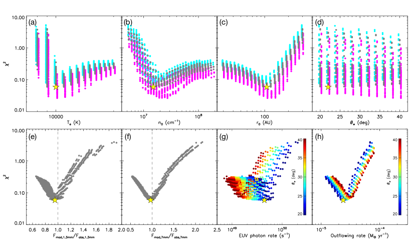
Appendix Figure 6: Distributions of $\chi^{2}$ values of free-free model fitting with model parameters: electron temperature $T_{\mathrm{e}}$ (panel a), central electron number density $n_{0}$ (panel b), radius of outflow launching region $\varpi_{0}$ (panel c), outflow half-opening angle $\theta_{w}$ (panel d), ratios of model and observed fluxes in the two bands (panels e and f), ionizing EUV photon rate (panel g), and outflowing rate assuming a velocity of $30~{}\mbox{km s}^{-1}$ (panel h). In panels a$-$f, cyan, magenta and grey symbols show the distributions of $\chi^{2}_{\mathrm{7mm}}$, $\chi^{2}_{\mathrm{1.3mm}}$ and $\chi^{2}_{\mathrm{tot}}=(\chi^{2}_{\mathrm{7mm}}+\chi^{2}_{\mathrm{1.3mm}})/2$ of the models, respectively. In panels a$-$d, the symbols are slightly offset in x-axis for better presentation. In panels e and f, the fluxes are integrated over the region with intensities $>0.1I_{\mathrm{obs,center}}$ (same as the region used in the 2D model fitting; see red contours in Figure 3). In panels g and h, only $\chi^{2}_{\mathrm{tot}}$ values are shown with the colors showing the half-opening angle parameter $\theta_{w}$. The yellow star marks the position of the best-fit model (minimum $\chi^{2}_{\mathrm{tot}}$).

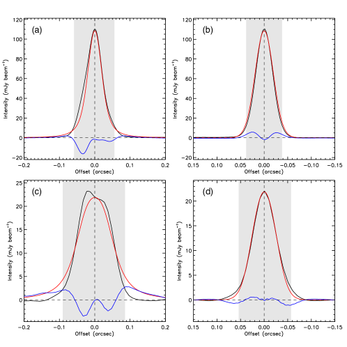
Appendix Figure 7: Comparison of the observed continuum intensity profiles with the model. (a): The observed 1.3 mm intensity profile along the outflow axis (black) compared with the model (red), with the residual shown in blue. The negative position offsets are to the south. (b): Same as panel a, but with the intensity profiles passing through the center and perpendicular to the outflow axis. The negative position offsets are to the west. (c)$-$(d): Same as panels a$-$b, but for the 7 mm continuum. The grey areas are with observed intensities $>0.1I_{\rm obs,center}$, which is used in the 2D fitting.

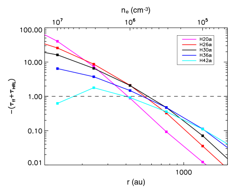
Appendix Figure 8: Dependence of total continuum and hydrogen recombination line optical depths $-(\tau_{\mathrm{ff}}+\tau_{\mathrm{HRL}})$ under non-LTE conditions on the distance from the center or the electron density, estimated based on the free-free emission model. Strong maser amplification requires $\tau_{\mathrm{ff}}+\tau_{\mathrm{HRL}}\ll-1$. Curves with different colors show different hydrogen recombination lines.

In addition to constraining the four free parameters, we also calculate the total fluxes, ionizing photon rates and mass outflow rates from the models, which are shown in panels e$-$h. Panels e and f show the comparison between the model and observation fluxes at 1.3 and 7 mm integrated in regions with observed intensities $>0.1I_{\mathrm{obs,center}}$ (same as the region used in the 2D model fitting). The model fluxes are slightly lower (within $5\%$) than the observed values. Panel g shows the ionizing photon rate, which is calculated following

$$S=4\pi\int_{\mathrm{axis}}\alpha_{B}n^{2}z^{2}dz,$$ (A5)

where $\alpha_{B}$ is the case B recombination rate for which we adopt the fitting formulas from Draine (2011), and the integration is along the axis from 0 to $\infty$. Note that this is only a lower limit for the ionizing photon luminosity in the outflow, which are just enough to ionize the outflow and ignore the possible effects of dust absorption. The uncertainty of the EUV photon rate is relatively large. Models with low $\chi^{2}$ values have EUV photon rates spanning from $\sim 1.4\times 10^{49}~{}\mathrm{s}^{-1}$ to $\sim 6\times 10^{49}~{}\mathrm{s}^{-1}$. The uncertainty is mostly from the weak constraint on the opening angle (and inclination), as shown in panel d. The best-fit model (minimum $\chi^{2}_{\mathrm{tot}}$) has an EUV photon rate of $4.5\times 10^{49}~{}\mathrm{s}^{-1}$, while the most probable inclination range ($55^{\circ}<i<90^{\circ}$, i.e. $35^{\circ}<\theta_{w}<40^{\circ}$) gives a range $1.4\times 10^{49}~{}\mathrm{s}^{-1}<S<1.8\times 10^{49}~{}\mathrm{s}^{-1}$. Panel h shows the mass outflow rates in the model (assuming a velocity of $30~{}\mbox{km s}^{-1}$; see §4.2). The best-fit models have rates from $2\times 10^{-5}(v/30~{}\mbox{km s}^{-1})~{}M_{\odot}~{}\mathrm{yr}^{-1}$ to $3.5\times 10^{-5}(v/30~{}\mbox{km s}^{-1})~{}M_{\odot}~{}\mathrm{yr}^{-1}$. These values are obtained assuming all the ions are H⁺ and the total mass is 1.4 times of the hydrogen mass. If we consider the He⁺ contributions to the free-free emission, the mass outflowing rates are $\sim 7\%$ lower than the above values, assuming a constant ratio of 0.08 between He⁺ and H⁺ throughout the ionized region.

The comparisons between the observations and best-fit model are shown in Figures 3 and 4, and the Appendix Figure 7, including the images in both bands and spectral index maps, the mm to radio SEDs, as well as intensity profiles along and perpendicular to the outflow axis. The best-fit model successfully reproduces the absolute values and relative distributions of emission intensities in both bands. The profiles perpendicular to the outflow axis are typically well fit, while some asymmetries or excesses along the outflow axis still remain. In particular, at $0.02\arcsec$ to the south, the observed 7 mm image shows an additional peak. At the same location, the observed 1.3 mm image also has a slight excess (see the residual curves in panels a and c of Appendix Figure 7). This may be caused by some substructures in the ionized outflow that are not taken into account in our model’s simple geometry and density distribution. It is also possible that this excess, stronger in the lower frequency, contains contributions of non-thermal synchrotron emission.

Here we briefly discuss whether the observed H30$\alpha$ maser can happen under the temperature and density conditions derived from the free-free model. Strong maser amplification requires the total continuum and HRL optical depth $\tau_{\mathrm{ff}}+\tau_{\mathrm{HRL}}\ll-1$ (Báez-Rubio et al. 2013). The non-LTE HRL absorption coefficient can be written as $\kappa_{\mathrm{HRL}}=b_{n}\beta_{mn}\kappa_{\mathrm{HRL,LTE}}$, with $\kappa_{\mathrm{HRL,LTE}}$ being the absorption coefficient under LTE conditions, and $b_{n}$ and $\beta_{mn}$ being the departure coefficients for the recombination line from electronic level $m$ to $n$ (e.g. $m=31,n=30$ for H30$\alpha$; Dupree & Goldberg 1970). We adopt the values of $b_{n}$ and $\beta_{mn}$ derived by Walmsley (1990), which are dependent on the electron temperature $T_{e}$ and density $n_{e}$. The non-LTE HRL optical depth is then $\tau_{\mathrm{HRL}}=\kappa_{\mathrm{HRL}}l=b_{n}\beta_{mn}\kappa_{\mathrm{HRL,LTE}}l$, with $l$ being the physical length scale. Toward the center, with $n_{e}=n_{0}=1.5\times 10^{7}~{}\mathrm{cm}^{-3}$ and $T_{e}=10,000~{}{\rm K}$ from the free-free model, and assuming the length scale $l=\varpi_{0}=110~{}\mbox{au}$ for a first-order estimation, we estimate $\tau_{\mathrm{HRL}}\approx-20$. The total continuum and HRL optical depth is then $\tau_{\mathrm{ff}}+\tau_{\mathrm{HRL}}\approx-19$, which is consistent with the observed strong maser amplification (Appendix Figure 8). We further estimate the distribution of non-LTE HRL optical depth over the ionized region, by adopting a simple relation $n_{e}\propto r^{-2}\sim l^{-2}$. The dependence of $\tau_{\mathrm{ff}}+\tau_{\mathrm{HRL}}$ on the distance to the center $r$ or the density distribution $n_{e}$ is shown in the Appendix Figure 8. Strong maser amplification appears constrained in the region $r\lesssim 400~{}\mbox{au}$ for H30$\alpha$ line, which is consistent with the observation that the high maser amplification is concentrated close to the disk mid-plane. It also shows that similar maser effects may be seen in HRLs from about H20$\alpha$ to about H42$\alpha$, which may be tested by future observations. However, accurate model prediction for HRL maser intensities is difficult as full consideration of the radiation field is need, which is out of the scope of this paper.

Appendix B Determining the H30$\alpha$ emission positional centroids.

The centroid positions are determined by fitting Gaussian ellipses to the H30$\alpha$ emissions observed in the C9 configuration at channels with peak intensities $>10\sigma$. The accuracy of the centroid positions are affected by the signal-to-noise ratio (S/N) of the data, following $\Delta\theta_{\mathrm{fit}}=\theta_{\mathrm{beam}}/(2~{}\mathrm{S/N})$ (Condon 1997), where $\theta_{\mathrm{beam}}$ is the resolution beam size, for which we adopt the major axis of the resolution beam $\theta_{\mathrm{beam}}=38~{}\mathrm{mas}$ (320 au). The phase noise in the bandpass calibrator also introduces an additional error to the centroid positions through passband calibrations (Zhang et al. 2017). The phase noise in the passband calibrator J2000-1748 is found to be $\Delta\phi=5.4^{\circ}$ after smoothing of 4 channels. Such smoothing is the same as that used in deriving the passband calibration solutions. The additional position error is $\Delta\theta_{\mathrm{bandpass}}=\theta_{\mathrm{beam}}(\Delta\phi/360^{\circ})$, and the uncertainties in the centroid positions are $\Delta\theta_{\mathrm{centroid}}=\sqrt{\Delta\theta_{\mathrm{fit}}^{2}+\Delta\theta_{\mathrm{bandpass}}^{2}}$.

Appendix C Estimating the Magnetic Field Strength from Synchrotron Emission

In the region with negative spectral indices indicating synchrotron emission, we estimate the minimum-energy magnetic filed strength, $B_{\mathrm{min}}$, which minimizes the total energy of the synchrotron source by assuming equipartition between the magnetic field energy and the particle energy. Following the classical formula for estimating minimum-energy magnetic field strength (e.g., Carrasco-González et al. 2010; Sanna et al. 2019)

$$B_{\mathrm{min}}=[4.5c_{12}(1+k)L_{R}]^{2/7}(R^{3})^{-2/7},$$ (C1)

where $L_{R}$ is the synchrotron luminosity, $R$ is the source radius, $k$ is the energy ratio between the ions (carrying most of the energy but not radiating significantly) and electrons, and $c_{12}$ is a coefficient dependent on the spectral index and the minimum and maximum frequencies in the integration of the spectrum. Here $B_{\mathrm{min}}$ is in Gauss, and $L_{R}$, $R$, $k$ and $c_{12}$ are in cgs units. We define the synchrotron emission region as the region with intensity spectral indices of $\alpha<-0.3$ and both 1.3 and 7 mm emissions $>5\sigma$. Here we only consider the negative spectral index regions within $\sim 0.2\arcsec$ from the center, as the 7 mm image is affected by strong sidelobe patterns further out from the central source. The areas of the regions to the north and south of the central source are $0.00021\mathrm{arcsec}^{2}$ and $0.0013\mathrm{arcsec}^{2}$, which correspond to effective radii of $R=0.008\arcsec$ and $0.020\arcsec$, which we use as the radii of the synchrotron emitting regions. Assuming all the 1.3 and 7 mm emissions from these regions are due to synchrotron emission, we obtain synchrotron fluxes of 0.041 and 0.070 mJy at 1.3 and 7 mm in the northern region, and 1.0 and 1.7 mJy at 1.3 and 7 mm in the southern region. Note that these are only upper limits for the synchrotron fluxes, as these regions only have negative spectral indices $\sim-0.3$ while typical synchrotron emission has a spectral index of $\sim-0.75$, suggesting there are both free-free and synchrotron contributions in these regions. However, the magnetic field strength is not very sensitive to the synchrotron flux (see Eq. C1). We then calculate synchrotron luminosities of $L_{R}=8.1\times 10^{29}~{}\mathrm{erg}~{}\mathrm{s}^{-1}$ and $L_{R}=2.0\times 10^{31}~{}\mathrm{erg}~{}\mathrm{s}^{-1}$ in the northern and southern regions, by integrating the synchrotron fluxes from 1.3 to 7 mm assuming a power-law distribution. For this frequency range, we obtain $c_{12}=3.2\times 10^{6}$ following Govoni & Feretti (2004), We also adopt $k=40$ following Carrasco-González et al. (2010) and Sanna et al. (2019). These values give $B_{\mathrm{min}}=15$ and 17 mG in the northern and southern regions, respectively.

References

- Anglada et al. (2018) Anglada, G., Rodríguez, L. F., and Carrasco-González, 2018, A&ARv, 26, 3
- Báez-Rubio et al. (2013) Báez-Rubio, A., Martín-Pintado, J., Thum, C., Planesas, P., 2013, A&A, 553, A45
- Beltrán et al. (2016) Beltrán, M. T., Cesaroni, R., Moscadelli, L., et al. 2016, A&A, 593, 49
- Briggs (1995) Briggs, D. S. 1995, in BAAS 27, Am. Astron. Soc. Meet. Abstr., 112.02
- Carrasco-González et al. (2010) Carrasco-González, C., Rodríguez, L. F., Anglada, G., et al. 2010, Science, 330, 1209
- Condon (1997) Condon, J. J. 1997, PASP, 109, 166
- De Buizer et al. (2005) De Buizer, J. M., Radomski, J. T., Telesco, C. M. & Piña, R. K. 2005, ApJS, 156, 179
- De Buizer et al. (2017) De Buizer, J. M., Liu, M., Tan, J. C., Zhang, Y., et al., 2017, ApJ, 843, 33
- Davies et al. (2011) Davies, B., Hoare, M. G., Lumsden, S. L., et al. 2011, MNRAS, 416, 972
- Draine (2011) Draine, B. T. 2011 Physics of the Interstellar and Intergalactic Medium (Princeton: Princeton Univ. Press)
- Dupree & Goldberg (1970) Dupree, A. K. & Goldberg, L. 1970, ARA&A, 8, 231
- Forster & Caswell (1989) Forster, J. R., & Caswell, J. L. 1989, A&A, 213, 339
- Hollenbach et al. (1994) Hollenbach, D., Johnstone, D., Lizano, S., & Shu, F. 1994, ApJ, 428, 654
- Garay et al. (1996) Garay, G., Ramirez, S., Rodriguez, L. F., et al. 1996, ApJ, 459,193
- Govoni & Feretti (2004) Govoni, F., & Feretti, L. 2004, Int. J. Mod. Phys. D, 13, 1549
- Hofmann et al. (2002) Hofmann, K.-H., Balega, Y., Ikhsanov, N. R., et al. 2002, A&A, 395, 891
- Jiménez-Serra et al. (2013) Jiménez-Serra, I., Báez-Rubio, A., Rivilla, V. M., et al. 2013, ApJL, 764, L4
- Krumholz et al. (2009) Krumholz, M. R., Klein, R. I., McKee, C. F., Offner, S. S. R., & Cunningham, A. J. 2009, Science, 323, 754
- Kuiper et al. (2010) Kuiper, R., Klahr, H., Beuther, H., & Henning, T. 2010, ApJ, 722, 1556
- Martín-Pintado et al. (1989) Martín-Pintado, J., Bachiller, R., Thum, C., Walmsley, M. 1989, A&A, 215, L13
- Matsushita et al. (2017) Matsushita, Y., Machida, M. N., Sakurai, Y., Hosokawa, T., 2017, MNRAS, 470, 1026
- McMullin et al. (2007) McMullin, J. P., Waters, B., Schiebel, D., Young, W., & Golap, K. 2007, Astronomical Data Analysis Software and Systems XVI (ASP Conf. Ser. 376), ed. R. A. Shaw, F. Hill, & D. J. Bell (San Francisco, CA: ASP), 127
- Moscadelli et al. (2013) Moscadelli, L., Cesaroni, R., Sánchez-Monge, Á., et al. 2013, A&A, 558, 145
- Moscadelli et al. (2018) Moscadelli, L., Rivilla, V. M., Cesaroni, R., et al. 2018, A&A, 616, A66
- Mottram et al. (2011) Mottram, J. C., Hoare, M. G., Davies, B., et al. 2011, ApJL, 730, L33
- Müller et al. (2005) Müller, H. S. P., Schlöder, F., Stutzki, J., Winnewisser, G. 2005, JMoSt, 742, 215
- Ossenkopf & Henning (1994) Ossenkopf, V., Henning, T. 1994, A&A, 291, 943
- Ortega et al. (2012) Ortega, M. E., Paron, S., Chichowolski, S. et al. 2012, A&A, 546, 96
- Padovani et al. (2015) Padovani, M., Hennebelle, P., Marcowith, A., Ferrière, K. 2015, A&A, 582, L13
- Padovani et al. (2016) Padovani, M., Marcowith, A., Hennebelle, P., Ferrière, K. 2016, A&A, 590, 8
- Paron et al. (2013) Paron, S., Fariña, C., & Ortega, M. E. 2013, A&A, 559, L2
- Peters et al. (2010) Peters, T., Banerjee, R., Klessen, R. S., et al. 2010, ApJ, 711, 1017
- Rosero et al. (2016) Rosero, V., Hofner, P., Claussen, M., et al., 2016, ApJS, 227, 25
- Rosero et al. (2019) Rosero, V., Tanaka, K. E. I., Tan, J. C., et al., 2019, ApJ, 873, 20
- Sanna et al. (2019) Sanna, A., Moscadelli, L., Goddi, C., et al., 2019, A&A, 623, L3
- Staff et al. (2019) Staff, J. E., Tanaka, K. E. I., Tan, J. C. 2019, ApJ, 882, 123
- Tan et al. (2014) Tan, J. C., Beltrán, M. T., Caselli, P., et al. 2014, in Protostars and Planets VI, ed. H. Beuther et al. (Tucson, AZ: Univ. Arizona Press), 149
- Tanaka & Nakamoto (2011) Tanaka, K. E. I., & Nakamoto, T. 2011, ApJ, 739, L50
- Tanaka et al. (2016) Tanaka, K. E. I., Tan, J. C., Zhang, Y. 2016, ApJ, 818, 52
- Tanaka et al. (2017) Tanaka, K. E. I., Tan, J. C., Zhang, Y. 2017, ApJ, 835, 32
- Torrelles et al. (2011) Torrelles, J. M., Patel, N. A., Curiel, S. et al. 2011, MNRAS, 410, 627
- Urquhart et al. (2009) Urquhart, J. S., Hoare, M. G., Purcell, C. R., et al. 2009, A&A, 501, 539
- Vlemmings et al. (2010) Vlemmings, W. H. T., Surcis, G., Torstensson, K. J. E., et al. 2010, MNRAS, 404, 134
- Walmsley (1990) Walmsley, C. M. 1990, A&AS, 82, 201
- Wilner et al. (1996) Wilner, D. J., Ho, P. T. P., Zhang, Q., 1996, ApJ, 462, 339
- Wilson et al. (2013) Wilson, T. L., Rohlfs, K., & Hüttemeister, S. 2013, Tools of Radio Astronomy (6th ed.; Berlin: Springer)
- Wolfire & Cassinelli (1987) Wolfire, M. G., & Cassinelli, J. P. 1987, ApJ, 319, 850
- Wood & Churchwell (1989) Wood, D. O. S. & Churchwell, E. 1989, ApJS, 69, 831
- Wu et al. (2019) Wu, Y. W., Reid, M. J., Sakai, N. et al. 2019, ApJ, 874, 94
- Yorke & Sonnhalter (2002) Yorke, H. W., & Sonnhalter, C. 2002, ApJ, 569, 846
- Zhang et al. (2017) Zhang, Q., Claus, B., Watson, L., Moran, J., 2017, ApJ, 837, 53
- Zhang & Tan (2018) Zhang, Y. & Tan, J. C. 2018, ApJ, 853, 18
- Zhang et al. (2019) Zhang, Y., Tan, J. C., Tanaka, K. E. I., et al. 2019, Nat. Astron., 3, 517