Subspace Estimation from Unbalanced and Incomplete Data Matrices: $\ell_{2,\infty}$ Statistical Guarantees

Abstract

This paper is concerned with estimating the column space of an unknown low-rank matrix $\bm{A}^{\star}\in\mathbb{R}^{d_{1}\times d_{2}}$, given noisy and partial observations of its entries. There is no shortage of scenarios where the observations — while being too noisy to support faithful recovery of the entire matrix — still convey sufficient information to enable reliable estimation of the column space of interest. This is particularly evident and crucial for the highly unbalanced case where the column dimension $d_{2}$ far exceeds the row dimension $d_{1}$, which is the focal point of the current paper.

We investigate an efficient spectral method, which operates upon the sample Gram matrix with diagonal deletion. While this algorithmic idea has been studied before, we establish new statistical guarantees for this method in terms of both $\ell_{2}$ and $\ell_{2,\infty}$ estimation accuracy, which improve upon prior results if $d_{2}$ is substantially larger than $d_{1}$. To illustrate the effectiveness of our findings, we derive matching minimax lower bounds with respect to the noise levels, and develop consequences of our general theory for three applications of practical importance: (1) tensor completion from noisy data, (2) covariance estimation / principal component analysis with missing data, and (3) community recovery in bipartite graphs. Our theory leads to improved performance guarantees for all three cases.

Keywords: spectral method, principal component analysis with missing data, tensor completion, covariance estimation, spectral clustering, leave-one-out analysis

1 Introduction

Consider the problem of estimating the column space of a low-rank matrix $\bm{A}^{\star}=[A_{i,j}^{\star}]_{1\leq i\leq d_{1},1\leq j\leq d_{2}}$, based on noisy and highly incomplete observations of its entries. To set the stage, suppose that we observe

$$A_{i,j}=A_{i,j}^{\star}+N_{i,j},\qquad\forall\left(i,j\right)\in\Omega,$$ (1)

where $\Omega\subseteq\left\{1,\cdots,d_{1}\right\}\times\left\{1,\cdots,d_{2}\right\}$ is the sampling set, and $A_{i,j}$ denotes the observed entry at location $\left(i,j\right)$, which is corrupted by noise $N_{i,j}$. In contrast to the classical matrix completion problem that aims to fill in all missing entries [CR09, KMO10a, CLC19, CC18b], the current paper focuses solely on estimating the column space of $\bm{A}^{\star}$, which is oftentimes a less stringent requirement.

Motivating applications.

A problem of this kind arises in numerous applications. We immediately point out several representative examples as follows, with precise descriptions postponed to Section 4.

• Tensor completion and estimation. Imagine we seek to estimate a low-rank symmetric tensor from partial observations of its entries [BM16, XYZ17, MS18], a task that spans various applications like visual data inpainting [LMWY13] and medical imaging [SHKM14]. Consider, for example, an order-$3$ tensor $\bm{T}^{\star}=\sum_{s=1}^{r}\bm{w}_{s}^{\star}\otimes\bm{w}_{s}^{\star}\otimes\bm{w}_{s}^{\star}\in\mathbb{R}^{d\times d\times d}$, where $\left\{\bm{w}_{s}^{\star}\right\}$ represents a collection of tensor factors. An alternative representation of $\bm{T}^{\star}$ can be obtained by unfolding the tensor of interest into a low-rank structured matrix $\bm{A}^{\star}\in\mathbb{R}^{d\times d^{2}}$. Consequently, estimation of the subspace spanned by $\left\{\bm{w}_{s}^{\star}\right\}$ from partial noisy entries of $\bm{T}^{\star}$ — which serves as a common and crucial step for tensor completion [MS18, CLPC19] — is equivalent to estimating the column space of $\bm{A}^{\star}$ from incomplete and noisy data; see Section 4.1 for details. Notably, the unfolded matrix becomes extremely fat as the dimension $d$ grows.

• Covariance estimation / principal component analysis with missing data. Suppose we have available a sequence of $n$ independent sample vectors $\left\{\bm{x}_{i}\in\mathbb{R}^{d}\right\}_{i=1}^{n}$, whose covariance matrix exhibits certain low-dimensional structure. Several statistical models fall in the same vein of this model, e.g. the generalized spiked model [BY12] and the factor model [FWZZ18]. An important task amounts to estimating the principal subspace of the covariance matrix of interest, possibly in the presence of missing data (where we only get to see highly incomplete entries of $\{\bm{x}_{i}\}$). If a substantial amount of data are missing, then individual sample vectors cannot possibly be recovered, thus enabling privacy protection for individual data. Fortunately, one might still hope to estimate the principal subspace, provided that a large number of sample vectors are queried (which might yield a fat data matrix $\bm{X}:=[\bm{x}_{1},\cdots,\bm{x}_{n}]$). See Section 4.2.

• Community recovery in bipartite graphs. Community recovery is often concerned with clustering a collection of individuals or nodes into different communities, based on similarities between pairs of nodes. In many complex networks, such pairwise interactions might only occur when the two nodes involved belong to two disjoint groups (denoted by $\mathcal{U}$ and $\mathcal{V}$ respectively). This calls for community recovery in bipartite networks (sometimes referred to as biclustering) [Dhi01, LCJ14, AHB14, ZA18]. As we shall detail in Section 4.3, the biclustering problem is tightly connected to subspace estimation; for instance, the column subspace of some bi-adjacency matrix $\bm{A}\in\mathbb{R}^{|\mathcal{U}|\times|\mathcal{V}|}$ (which is a noisy copy of a low-rank matrix) reveals the community memberships in $\mathcal{U}$. When the size of $\mathcal{V}$ is substantially larger than that of $\mathcal{U}$, one might encounter a situation where only the nodes in $\mathcal{U}$ (rather than those in $\mathcal{V}$) can be reliably clustered. This calls for development of “one-sided” community recovery algorithms, that is, the type of algorithms that guarantee reliable clustering of $\mathcal{U}$ without worrying about the clustering accuracy in $\mathcal{V}$.

Contributions.

Since we concentrate primarily on estimating the column space of $\bm{A}^{\star}$, it is natural to expect a reduced sample complexity as well as a weaker requirement on the signal-to-noise ratio, in comparison to the conditions required for reliable reconstruction of the whole matrix — particularly for those highly unbalanced problems with drastically different dimensions $d_{1}$ and $d_{2}$. Focusing on a spectral method applied to the Gram matrix $\bm{A}\bm{A}^{\top}$ with diagonal deletion (whose variants have been studied in multiple contexts [Lou14, FP16, LW12, MS18, EvdG19]), we establish new statistical guarantees in terms of the sample complexity and the estimation accuracy, both of which strengthen prior theory. Our results deliver optimal $\ell_{2,\infty}$ estimation risk bounds with respect to the noise level, which are previously unavailable. All this is accomplished via a powerful leave-one-out / leave-two-out analysis framework. Further, we develop minimax lower bounds under Gaussian noise, revealing that the sample complexity and the signal-to-noise ratio (SNR) required for spectral methods to achieve consistent estimation are both minimax optimal (up to some logarithmic factor). Finally, we develop concrete consequences of our general theory for all three applications mentioned above, leading to optimal performance guarantees that improve upon prior literature.

It is worth noting that low-rank subspace estimation from noisy and incomplete data has been extensively studied in a large number of prior work (e.g. [Lou14, AFWZ17, CKR17, ZCW18, ZWS19]). While many of these prior results allow $d_{1}$ and $d_{2}$ to differ, they typically fall short of establishing optimal dependency on $d_{1}$ and $d_{2}$ in the highly unbalanced scenarios. The focal point of this paper is thus to characterize the effect of such unbalancedness (as reflected by the aspect ratio $d_{2}/d_{1}$) upon consistent subspace estimation.

Paper organization.

The rest of this paper is organized as follows. Section 2 formulates the problem and introduces basic definitions and notations. In Section 3, we present our theoretical guarantees for a spectral method, as well as minimax lower bounds. Section 4 applies our general theorem to the aforementioned applications, and corroborate our theory by numerical experiments. Section 5 provides an overview of related prior works. The proof of our main theory is outlined in Section 6, with the proofs of many auxiliary lemmas postponed to the appendix. We conclude the paper with a discussion of future directions in Section 7.

2 Problem formulation

2.1 Models

Low-rank matrix.

Suppose that the unknown matrix $\bm{A}^{\star}\in\mathbb{R}^{d_{1}\times d_{2}}$ is rank-$r$, where the row dimension $d_{1}$ and the column dimension $d_{2}$ are allowed to be drastically different. Assume that the (compact) singular value decomposition (SVD) of $\bm{A}^{\star}$ is given by

$$\bm{A}^{\star} =\bm{U}^{\star}\bm{\Sigma}^{\star}\bm{V}^{\star\top}=\sum_{i=1}^{r}\sigma_{i}^{\star}\bm{u}_{i}^{\star}\bm{v}_{i}^{\star\top}.$$ (2)

Here, $\sigma_{1}^{\star}\geq\sigma_{2}^{\star}\geq\cdots\geq\sigma_{r}^{\star}>0$ represent the $r$ nonzero singular values of $\bm{A}^{\star}$, and $\bm{\Sigma}^{\star}\in\mathbb{R}^{r\times r}$ is a diagonal matrix whose diagonal entries are given by $\{\sigma_{1}^{\star},\cdots,\sigma_{r}^{\star}\}$. The columns of $\bm{U}^{\star}=\left[\bm{u}_{1}^{\star},\cdots,\bm{u}_{r}^{\star}\right]\in\mathbb{R}^{d_{1}\times r}$ (resp. $\bm{V}^{\star}=\left[\bm{v}_{1}^{\star},\cdots,\bm{v}_{r}^{\star}\right]\in\mathbb{R}^{d_{2}\times r}$) are orthonormal, which are the top-$r$ left (resp. right) singular vectors of $\bm{A}^{\star}$. We define and denote the condition number of $\bm{A}^{\star}$ as follows

$$\kappa:=\sigma_{1}^{\star}\,/\,\sigma_{r}^{\star},$$ (3)

and take

$$d:=\max\left\{d_{1},d_{2}\right\}.$$ (4)

Incoherence.

Further, we impose certain incoherence conditions on the unknown matrix $\bm{A}^{\star}$, which are commonly adopted in the matrix completion literature (e.g. [CR09, KMO10a, CLC19]).

Definition 1 (Incoherence parameters).

Define the incoherence parameters $\mu_{0}$, $\mu_{1}$ and $\mu_{2}$ as follows

$$\mu_{0}:=\frac{d_{1}d_{2}\underset{1\leq i\leq d_{1},1\leq j\leq d_{2}}{\max}\left|A_{i,j}^{\star}\right|^{2}}{\left\|\bm{A}^{\star}\right\|_{\mathrm{F}}^{2}}$$ , (5)

$$\mu_{1}:=\frac{d_{1}}{r}\max_{1\leq i\leq d_{1}}\left\|\bm{U}^{\star\top}\bm{e}_{i}\right\|_{2}^{2}\qquad \text{and}\qquad\mu_{2}:=\frac{d_{2}}{r}\max_{1\leq i\leq d_{2}}\left\|\bm{V}^{\star\top}\bm{e}_{i}\right\|_{2}^{2},$$ (6)

where $\bm{e}_{i}$ is the $i$-th standard basis vector of compatible dimensionality.

Intuitively, when $\mu_{0}$, $\mu_{1}$ and $\mu_{2}$ are all small, the energies of the matrices $\bm{A}^{\star}$, $\bm{U}^{\star}$ and $\bm{V}^{\star}$ are (nearly) evenly spread out across all entries, rows, and columns. For notational simplicity, we shall set

$$\mu:=\max\left\{\mu_{0},\mu_{1},\mu_{2}\right\}.$$ (7)

Random sampling and random noise.

Suppose that we have only collected noisy observations of the entries of $\bm{A}^{\star}$ over a sampling set $\Omega\subseteq\{1,\cdots,d_{1}\}\times\{1,\cdots,d_{2}\}$. Specifically, we observe

$$A_{i,j}=\begin{cases}A_{i,j}^{\star}+N_{i,j},\qquad&(i,j)\in\Omega,\\ 0,&\text{else},\end{cases}$$ (8)

where $N_{i,j}$ denotes the noise at location $(i,j)$. For notational simplicity, we shall write

$$\bm{A}=\mathcal{P}_{\Omega}(\bm{A}) =\mathcal{P}_{\Omega}(\bm{A}^{\star})+\mathcal{P}_{\Omega}(\bm{N}),$$ (9)

where $\mathcal{P}_{\Omega}$ represents the Euclidean projection onto the subspace of matrices supported on $\Omega$. In addition, this paper concentrates on random sampling and random noise as follows.

Assumption 1 (Random sampling).

Each $(i,j)$ is included in the sampling set $\Omega$ independently with probability $p$.

Assumption 2 (Random noise).

The noise $N_{i,j}$’s are independent random variables and satisfy the following conditions: for each $1\leq i\leq d_{1},1\leq j\leq d_{2}$,

• (Zero mean) $\mathbb{E}\left[N_{i,j}\right]=0$;

• (Variance) $\mathsf{Var}\left(N_{i,j}\right)\leq\sigma^{2}$;

• (Magnitude) Each $N_{i,j}$ satisfies either of the following condition:

  • $\left|N_{i,j}\right|\leq R$;

  • $N_{i,j}$ has a symmetric distribution satisfying $\mathbb{P}\left\{\left|N_{i,j}\right|>R\right\}\leq c_{\mathrm{r}}d^{-12}$ for some universal constant $c_{\mathrm{r}}>0$.

  Here, $R$ is some quantity obeying

  $$\frac{R^{2}}{\sigma^{2}}\leq C_{\mathrm{r}}\frac{\min\left\{p\sqrt{d_{1}d_{2}},\,pd_{2}\right\}}{\log d}$$ (10)

  for some universal constant $C_{\mathrm{r}}>0$.

As a remark, Assumption 2 allows the largest possible size $R$ of each noise component to be substantially larger than its typical size $\sigma$. For example, if $p\asymp 1$, then $R$ can be $\min{\{(d_{1}d_{2})^{1/4},\sqrt{d_{2}}\}}$ times larger than $\sigma$ (ignoring any logarithmic factor). In addition, the noise $N_{i,j}$’s do not necessarily have identical variance; in fact, our formulation allows us to accommodate the heteroscedasticity of noise (i.e. the scenario where the noise has location-varying variance).

Goal.

Given incomplete and noisy observations about $\bm{A}^{\star}\in\mathbb{R}^{d_{1}\times d_{2}}$ (cf. (8)), we seek to estimate $\bm{U}^{\star}\in\mathbb{R}^{d_{1}\times r}$ modulo some global rotation. We emphasize once again that the aim here is not to estimate the entire matrix. In truth, there are many unbalanced cases with $d_{2}\gg d_{1}$ such that (1) reliable estimation of $\bm{U}^{\star}$ is feasible, but (2) faithful estimation of the whole matrix $\bm{A}^{\star}$ is information theoretically impossible.

2.2 Notation

We denote $\left[n\right]:=\{1,\cdots,n\}$. For any matrix $\bm{A}\in\mathbb{R}^{d_{1}\times d_{2}}$, we use $\sigma_{i}\left(\bm{A}\right)$ and $\lambda_{i}\left(\bm{A}\right)$ to represent the $i$-th largest singular value and the $i$-th largest eigenvalue of $\bm{A}$, respectively. Let $\bm{A}_{i,:}$ and $\bm{A}_{:,j}$ denote respectively the $i$-th row and the $j$-th column of $\bm{A}$. Let $\left\|\bm{A}\right\|$ (resp. $\left\|\bm{A}\right\|_{\mathrm{F}}$) represent the spectral norm (resp. the Frobenius norm) of $\bm{A}$. We also denote by $\left\|\bm{A}\right\|_{2,\infty}:=\max_{i\in[d_{1}]}\|\bm{A}_{i,:}\|_{2}$ and $\left\|\bm{A}\right\|_{\infty}:=\max_{i\in[d_{1}],j\in[d_{2}]}\big{|}A_{i,j}\big{|}$ the $\ell_{2,\infty}$ norm and the entrywise $\ell_{\infty}$ norm of $\bm{A}$, respectively. Similarly, for any tensor $\bm{T}$, we use $\|\bm{T}\|_{\infty}$ to represent the largest magnitude of the entries of $\bm{T}$. Moreover, we denote by $\mathcal{P}_{\mathsf{diag}}$ the projection onto the subspace that vanish outside the diagonal, and define $\mathcal{P}_{\mathsf{off}\text{-}\mathsf{diag}}$ such that $\mathcal{P}_{\mathsf{off}\text{-}\mathsf{diag}}(\bm{A}):=\bm{A}-\mathcal{P}_{\mathsf{diag}}(\bm{A})$. Let $\mathcal{O}^{r\times r}$ stand for the set of $r\times r$ orthonormal matrices. In addition, we use $\mathsf{diag}\left(\bm{a}\right)$ to represent a diagonal matrix whose $(i,i)$-th entry is equal to $a_{i}$. Throughout this paper, the notations $C,C_{1},\cdots,c,c_{1},\cdots$ denote absolute positive constants whose values may change from line to line.

Furthermore, for any real-valued functions $f(d_{1},d_{2})$ and $g(d_{1},d_{2})$, $f(d_{1},d_{2})\lesssim g(d_{1},d_{2})$ or $f(d_{1},d_{2})=O\left(g(d_{1},d_{2})\right)$ mean that $\left|f(d_{1},d_{2})/g(d_{1},d_{2})\right|\leq C_{1}$ for some constant $C_{1}>0$; $f(d_{1},d_{2})\gtrsim g(d_{1},d_{2})$ means that $\left|f(d_{1},d_{2})/g(d_{1},d_{2})\right|\geq C_{2}$ for some universal constant $C_{2}>0$; $f(d_{1},d_{2})\asymp g(d_{1},d_{2})$ means that $C_{1}\leq\left|f(d_{1},d_{2})/g(d_{1},d_{2})\right|\leq C_{2}$ for some universal constants $C_{1},C_{2}>0$; $f(d_{1},d_{2})=o\left(g(d_{1},d_{2})\right)$ means that $f(d_{1},d_{2})/g(d_{1},d_{2})\rightarrow 0$ as $\min\left\{d_{1},d_{2}\right\}\rightarrow\infty$. In addition, $f(d_{1},d_{2})\ll g(d_{1},d_{2})$ (resp. $f(d_{1},d_{2})\gg g(d_{1},d_{2})$) means that there exists some sufficiently small (resp. large) constant $c_{1}>0$ (resp. $c_{2}>0$) such that $f(d_{1},d_{2})\leq c_{1}g(d_{1},d_{2})$ (resp. $f(d_{1},d_{2})\geq c_{2}g(d_{1},d_{2})$) holds true for all sufficiently large $d_{1}$ and $d_{2}$.

3 Main results

3.1 Algorithm: a spectral method with diagonal deletion

Recall that $\bm{A}=[A_{i,j}]_{1\leq i\leq d_{1},1\leq j\leq d_{2}}$ is the zero-padded data matrix (see (8)). It is easily seen that, under our random sampling model (i.e. Assumption 1), $p^{-1}\bm{A}$ serves as an unbiased estimator of $\bm{A}^{\star}$. One might thus expect the left singular subspace of $\bm{A}$ to form a reasonably good estimator of the subspace spanned by $\bm{U}^{\star}$. As it turns out, when $\bm{A}^{\star}$ is a very fat matrix (namely, $d_{2}\gg d_{1}$), this approach might fail to work when the sample complexity is not sufficiently large or when the noise size is not sufficiently small.

This paper adopts an alternative route by resorting to the sample Gram matrix $\bm{A}\bm{A}^{\top}$ (properly rescaled). Straightforward calculation reveals that

$$\frac{1}{p^{2}}\mathbb{E}\left[\bm{A}\bm{A}^{\top}\right]=\bm{A}^{\star}\bm{A}^{\star\top}+\underset{\text{a diagonal matrix}}{\underbrace{\left(\frac{1}{p}-1\right)\mathcal{P}_{\mathsf{diag}}\left(\bm{A}^{\star}\bm{A}^{\star\top}\right)+\frac{1}{p}\mathsf{\mathsf{diag}}\Bigg{(}\Bigg{[}\sum_{j=1}^{d_{2}}\mathsf{Var}(N_{i,j})\Bigg{]}_{1\leq i\leq d_{1}}\Bigg{)}}},$$ (11)

where $\mathsf{diag}\left(\bm{a}\right)$ with $\bm{a}\in\mathbb{R}^{d_{1}}$ represents a diagonal matrix whose $(i,i)$-th entry equals $a_{i}$. The identity (11) implies that the diagonal components of $p^{-2}\mathbb{E}\left[\bm{A}\bm{A}^{\top}\right]$ are significantly inflated, which might need to be properly suppressed.

In order to remedy the above-mentioned diagonal inflation issue, we adopt a simple strategy that zeros out all diagonal entries; that is, performing the spectral method on the following matrix

$$\bm{G}=\frac{1}{p^{2}}\mathcal{P}_{\mathsf{off}\text{-}\mathsf{diag}}\big{(}\bm{A}\bm{A}^{\top}\big{)}$$ (12)

with $\mathcal{P}_{\mathsf{off}\text{-}\mathsf{diag}}(\bm{M}):=\bm{M}-\mathcal{P}_{\mathsf{diag}}(\bm{M})$ denoting projection onto the set of zero-diagonal matrices. This clearly satisfies

$$\mathbb{E}\left[\bm{G}\right]=\mathcal{P}_{\mathsf{off}\text{-}\mathsf{diag}}\left(\bm{A}^{\star}\bm{A}^{\star\top}\right)=\mathcal{P}_{\mathsf{off}\text{-}\mathsf{diag}}\left(\bm{U}^{\star}\bm{\Sigma}^{\star 2}\bm{U}^{\star\top}\right).$$

If the diagonal entries of $\bm{A}^{\star}\bm{A}^{\star\top}$ are not too large, then one has $\bm{A}^{\star}\bm{A}^{\star\top}\approx\mathcal{P}_{\mathsf{off}\text{-}\mathsf{diag}}\left(\bm{A}^{\star}\bm{A}^{\star\top}\right)$ and, as a result, the rank-$r$ eigen-subspace of $\bm{G}$ might form a reliable estimate of the subspace spanned by $\bm{U}^{\star}$. The procedure is summarized in Algorithm 1.

Algorithm 1 The spectral method on the diagonal-deleted Gram matrix

1:  Input: sampling set $\Omega$, observed entries $\left\{A_{i,j}\mid\left(i,j\right)\in\Omega\right\}$, sampling rate $p$, rank $r$.

2:  Compute the (truncated) rank-$r$ eigen-decomposition $\bm{U}\bm{\Lambda}\bm{U}^{\top}$ of $\bm{G}$, where $\bm{U}\in\mathbb{R}^{d_{1}\times r}$, $\bm{\Lambda}\in\mathbb{R}^{r\times r}$, and

$$\bm{G}:=\mathcal{P}_{\mathsf{off}\text{-}\mathsf{diag}}\left(\tfrac{1}{p^{2}}\bm{A}\bm{A}^{\top}\right).$$ (13)

Here, $\bm{A}$ is defined in (9) and $\mathcal{P}_{\mathsf{off}\text{-}\mathsf{diag}}\left(\bm{M}\right)$ zeros out the diagonal entries of a matrix $\bm{M}$.

3:  Output $\bm{U}$ as the subspace estimate, and $\bm{\Sigma}=\bm{\Lambda}^{1/2}$ as the spectrum estimate.

We remark that this is clearly not a new algorithmic idea. In fact, proper handling of the diagonal entries (e.g. diagonal deletion, diagonal reweighting) has already been recommended in several different applications, including bipartite stochastic block models [FP16], covariance estimation [Lou13, Lou14, LW12, EvdG19], tensor completion [MS18], to name just a few.

3.2 Theoretical guarantees

In general, one can only hope to estimate $\bm{U}^{\star}$ up to global rotation. With this in mind, we introduce the following rotation matrix

$$\bm{R}\,:=\,\underset{\bm{Q}\in\mathcal{O}^{r\times r}}{\arg\min}\text{ }\left\|\bm{U}\bm{Q}-\bm{U}^{\star}\right\|_{\mathrm{F}},$$ (14)

where $\mathcal{O}^{r\times r}$ stands for the set of $r\times r$ orthonormal matrices. In words, $\bm{R}$ is the global rotation matrix that best aligns $\bm{U}$ and $\bm{U}^{\star}$. Equipped with this notation, the following theorem delivers upper bounds on the difference between the obtained estimate $\bm{U}$ and the ground truth $\bm{U}^{\star}$. The proof is postponed to Section 6.

Theorem 1.

Assume that the following conditions hold

$$p\geq c_{0}\max\left\{\frac{\mu\kappa^{4}r\log^{2}d}{\sqrt{d_{1}d_{2}}},\frac{\mu\kappa^{8}r\log^{2}d}{d_{2}}\right\},\,\,\frac{\sigma}{\sigma_{r}^{\star}}\leq c_{1}\min\left\{\frac{\sqrt{p}}{\kappa\sqrt[4]{d_{1}d_{2}}\,\sqrt{\log d}},\frac{1}{\kappa^{3}}\sqrt{\frac{p}{d_{1}\log d}}\right\}\,\,\text{and}\,\,r\leq\frac{c_{2}d_{1}}{\mu_{1}\kappa^{4}},$$ (15)

where $c_{0}>0$ is some sufficiently large constant and $c_{1},c_{2}>0$ are some sufficiently small constants. Then with probability at least $1-O\left(d^{-10}\right)$, the matrices $\bm{U}$ and $\bm{\Sigma}$ returned by Algorithm 1 satisfy

$$\left\|\bm{U}\bm{R}-\bm{U}^{\star}\right\| \lesssim\mathcal{E}_{\mathsf{general}},$$ (16a)

$$\left\|\bm{U}\bm{R}-\bm{U}^{\star}\right\|_{2,\infty} \lesssim\kappa^{2}\sqrt{\frac{\mu r}{d_{1}}}\cdot\mathcal{E}_{\mathsf{general}},$$ (16b)

$$\left\|\bm{\Sigma}-\bm{\Sigma}^{\star}\right\| \lesssim\sigma_{r}^{\star}\cdot\mathcal{E}_{\mathsf{general}},$$ (16c)

where $\bm{R}$ is defined in (14), and

$$\mathcal{E}_{\mathsf{general}}:=\underset{\mathrm{missing}\text{ }\mathrm{data}\text{ }\mathrm{effect}}{\underbrace{\frac{\mu\kappa^{2}r\log d}{\sqrt{d_{1}d_{2}}\,p}+\sqrt{\frac{\mu\kappa^{4}r\log d}{d_{2}p}}}}+\underset{\mathrm{noise}\text{ }\mathrm{effect}}{\underbrace{\frac{\sigma^{2}}{\sigma_{r}^{\star 2}}\frac{\sqrt{d_{1}d_{2}}\,\log d}{p}+\frac{\sigma\kappa}{\sigma_{r}^{\star}}\sqrt{\frac{d_{1}\log d}{p}}}}+\underset{\mathrm{diagonal}\text{ }\mathrm{deletion}\text{ }\mathrm{effect}}{\underbrace{\frac{\mu_{1}\kappa^{2}r}{d_{1}}}}.$$ (17)

Remark 1.

If there is no missing data, namely, $p=1$, then Theorem 1 continues to hold if the first two terms on the right-hand side of (17) are removed.

In a nutshell, Theorem 1 asserts that Algorithm 1 produces reliable estimates of the column subspace of $\bm{A}^{\star}$ — with respect to both the spectral norm and the $\left\|\cdot\right\|_{2,\infty}$ norm — under certain conditions imposed on the sample size and the noise size. For instance, consider the settings where $\mu,\kappa\asymp 1$ and $r\ll d_{1}\leq d_{2}$. Then as long as the following condition holds:

$$p\gtrsim\frac{r\log^{2}d}{\sqrt{d_{1}d_{2}}}\qquad\text{and}\qquad\frac{\sigma^{2}}{\sigma_{r}^{\star 2}}=o\left(\frac{p}{\sqrt{d_{1}d_{2}}\,{\log d}}\right),$$ (18)

the proposed spectral method achieves consistent estimation with high probability, namely,

$$\underset{\bm{Q}\in\mathcal{O}^{r\times r}}{\min}\frac{\left\|\bm{U}\bm{Q}-\bm{U}^{\star}\right\|}{\|\bm{U}^{\star}\|}=o\left(1\right),\quad\underset{\bm{Q}\in\mathcal{O}^{r\times r}}{\min}\frac{\left\|\bm{U}\bm{Q}-\bm{U}^{\star}\right\|_{2,\infty}}{\|\bm{U}^{\star}\|_{2,\infty}}=o\left(1\right)\quad\text{and}\quad\frac{\left\|\bm{\Sigma}-\bm{\Sigma}^{\star}\right\|}{\|\bm{\Sigma}^{\star}\|}=o\left(1\right).$$ (19)

Our upper bound (17) on the spectral norm error contains five terms. The first two terms of (17) are incurred by missing data; the third and the fourth terms of (17) represent the influence of observation noise; and the last term of (17) arises due to the bias caused by diagonal deletion. In particular, the last term is expected to be vanishingly small in the low-rank and incoherent case. Interestingly, both the missing data effect and the noise effect are captured by two different terms, which we shall interpret in what follows. Note that a primary focus of this paper is to demonstrate the feasibility of obtaining a tight control of the $\ell_{2,\infty}$ statistical error. This is particularly evident for the low-rank, incoherent, and well-conditioned case with $r,\mu,\kappa=O(1)$, in which our theory (cf. (16a) and (16b)) reveals that the $\ell_{2,\infty}$ error can be a factor of $\sqrt{1/d_{1}}$ smaller than the spectral norm error. The discussion below focuses on this case (namely, $r,\mu,\kappa=O(1)$), with all logarithmic factors omitted for simplicity of presentation.

• Let us first examine the influence of observation noise, which reads

  $$\frac{\sigma^{2}}{\sigma_{r}^{\star 2}}\frac{\sqrt{d_{1}d_{2}}}{p}+\frac{\sigma}{\sigma_{r}^{\star}}\sqrt{\frac{d_{1}}{p}}.$$ (20)

  This contains a quadratic term as well as a linear term w.r.t. $\sigma/\sigma_{r}^{\star}$. To interpret this, consider, for example, the case without missing data (i.e. $p=1$) and decompose

  $$\bm{A}\bm{A}^{\top}=\bm{A}^{\star}\bm{A}^{\star\top}+\underset{\text{linear perturbation}}{\underbrace{\bm{A}^{\star}\bm{N}^{\top}+\bm{N}\bm{A}^{\star\top}}}+\underset{\text{quadratic perturbation}}{\underbrace{\bm{N}\bm{N}^{\top}}},$$

  which clearly explains why eigenspace perturbation bounds depend both linearly and quadratically on the noise magnitudes. In general, the quadratic term $\frac{\sigma^{2}}{\sigma_{r}^{\star 2}}\frac{\sqrt{d_{1}d_{2}}}{p}$ is dominant when the signal-to-noise ratio (SNR) is not large enough; as the noise decreases to a sufficiently low level, the linear term starts to enter the picture. See Table 1 for a more precise summary. As we shall demonstrate momentarily, the terms (20) match the minimax limits (up to some logarithmic factor), meaning that it is generally impossible to get rid of either the linear term or the quadratic term.

  	large-noise regime (i.e. $\sigma/\sigma_{r}^{\star}\gtrsim\sqrt{p/d_{2}}$)	small-noise regime (i.e. $\sigma/\sigma_{r}^{\star}\lesssim\sqrt{p/d_{2}}$)
  dominant term	$\frac{\sigma^{2}}{\sigma_{r}^{\star 2}}\frac{\sqrt{d_{1}d_{2}}}{p}$	$\frac{\sigma}{\sigma_{r}^{\star}}\sqrt{\frac{d_{1}}{p}}$

  Table 1: The dominant term of the noise effect in $\frac{\sigma^{2}}{\sigma_{r}^{\star 2}}\frac{\sqrt{d_{1}d_{2}}}{p}+\frac{\sigma}{\sigma_{r}^{\star}}\sqrt{\frac{d_{1}}{p}}$ if $d_{2}\geq d_{1}$ (omitting logarithmic factors and assuming $r,\kappa,\mu\asymp 1$).

• Next, we examine the influence of missing data and assume $\sigma=0$ to simplify the discussion. If we view $\bm{N}_{\mathrm{missing}}=\frac{1}{p}\bm{A}-\bm{A}^{\star}$ as a zero-mean perturbation matrix, then one can write

  $$\tfrac{1}{p^{2}}\bm{A}\bm{A}^{\top}=\bm{A}^{\star}\bm{A}^{\star\top}+\underset{\text{linear perturbation}}{\underbrace{\bm{A}^{\star}\bm{N}_{\mathrm{missing}}^{\top}+\bm{N}_{\mathrm{missing}}\bm{A}^{\star\top}}}+\underset{\text{quadratic perturbation}}{\underbrace{\bm{N}_{\mathrm{missing}}\bm{N}_{\mathrm{missing}}^{\top}}}.$$

  Similar to the above noisy case with $p=1$, this decomposition explains why the influence of missing data contains two terms as well (see Table 2)

  $$\underset{\text{quadratic term in }1/\sqrt{p}}{\underbrace{\frac{1}{\sqrt{d_{1}d_{2}}\,p}}}+\underset{\text{linear term in }1/\sqrt{p}}{\underbrace{\frac{1}{\sqrt{d_{2}p}}}}.$$

  	high-missingness regime (i.e. $p\lesssim 1/d_{1}$)	low-missingness regime (i.e. $p\gtrsim 1/d_{1}$)
  dominant term	$\frac{1}{\sqrt{d_{1}d_{2}}\,p}$	$\frac{1}{\sqrt{d_{2}p}}$

  Table 2: The dominant term of the missing data effect in $\frac{1}{\sqrt{d_{1}d_{2}}\,p}+\frac{1}{\sqrt{d_{2}p}}$ if $d_{2}\geq d_{1}$ (omitting logarithmic factors and assuming $r,\kappa,\mu\asymp 1$).

Comparison with prior results.

To demonstrate the effectiveness of our theory, we take a moment to compare them with several prior results. Once again, the discussion below focuses on the case with $\max\left\{\mu,\kappa,r\right\}\asymp 1$. To be fair, it is worth noting that most papers discussed below either have different objectives (e.g. aiming at matrix estimation rather than subspace estimation [KMO10a, CT10, CCF⁺19]), or work with different (and possibly more general) model assumptions (e.g. square matrices [AFWZ17], or heteroskedastic noise [ZCW18]). Our purpose here is not to argue that our results are always stronger than the previous ones, but rather to point out the insufficiency of prior theory when directly applied to some basic settings.

• To begin with, we compare our spectral norm bound with that required for matrix completion [KMO10a, CT10, AFWZ17, CLC19, CCF⁺19] in the noise-free case (i.e. $\sigma=0$), in order to show how much saving can be harvested when we move from matrix estimation to subspace estimation. Suppose that $d_{2}\geq d_{1}$. As is well known, for both spectral and optimization-based methods, the sample complexities required for faithful matrix completion need to satisfy $pd_{1}d_{2}\gtrsim d_{2}\mathrm{poly}\log d$. In comparison, faithful estimation of the column subspace becomes feasible under the sample size $pd_{1}d_{2}\gtrsim\sqrt{d_{1}d_{2}}\,\mathrm{poly}\log d$, which can be much lower than that required for matrix completion (i.e. by a factor of $\sqrt{d_{2}/d_{1}}$). Further, we compare our $\|\cdot\|_{2,\infty}$ bound with the theory derived in [AFWZ17] when $d_{2}\gtrsim d_{1}\log^{2}d$. The theory in [AFWZ17, Theorem 3.4] requires the sample size and the noise level to satisfy $p\gtrsim d_{1}^{-1}\log d$ and $\sigma/\sigma_{r}^{\star}\lesssim\sqrt{\frac{p}{d_{2}\log d}}$, both of which are more stringent requirements than ours (namely, $p\gtrsim\frac{\log^{2}d}{\sqrt{d_{1}d_{2}}}$ and $\sigma/\sigma_{r}^{\star}\lesssim\frac{\sqrt{p}}{\sqrt[4]{d_{1}d_{2}}\,\sqrt{\log d}}$). Again, this arises primarily because [AFWZ17] seeks to estimate the whole matrix as opposed to its column subspace.

• We then compare our results with [MS18], which studies a diagonal-rescaling algorithm for the noise-free case (i.e. $\sigma=0$). Combining [MS18, Theorem 6.2] with the standard Davis-Kahan matrix perturbation theory, we can easily see that their spectral norm bound for subspace estimation reads

  $$\frac{\mathrm{poly}\log d}{\sqrt{d_{1}d_{2}}\,p}+\frac{\mathrm{poly}\log d}{\sqrt{d_{2}p}}.$$

  This coincides with our bound except for the last term of (17) (due to the bias incurred by diagonal deletion). In comparison, our theory offers additional $\ell_{2,\infty}$ statistical guarantees and covers the noisy case, thus strengthening the theory presented in [MS18].

• Additionally, we compare our spectral norm bound with the results derived in [ZCW18]. Consider the noiseless case where $\sigma=0$. It is proven in [ZCW18, Theorem 6] (see also the remark that follows) that: if the sample size satisfies $pd_{1}d_{2}\gtrsim\max\big{\{}d_{1}^{1/3}d_{2}^{2/3},d_{1}\big{\}}\mathrm{poly}\log d$, then the $\mathsf{HeteroPCA}$ estimator is consistent in estimating the column subspace (namely, achieving a relative $\ell_{2}$ estimation error not exceeding $o(1)$). In comparison, our theory claims that Algorithm 1 is guaranteed to yield consistent column subspace estimation as long as the sample size obeys $pd_{1}d_{2}\gtrsim\sqrt{d_{1}d_{2}}\,\mathrm{poly}\log d$. Consequently, if we omit logarithmic terms, then our sample complexity improves upon the theoretical support of $\mathsf{HeteroPCA}$ by a factor of $(d_{2}/d_{1})^{1/6}$ if $d_{2}\geq d_{1}$. Once again, the comparison here focuses on the effect of the aspect ratio $d_{2}/d_{1}$, without accounting for the influence of other parameters like $\mu,\kappa,r$.

SVD applied directly to $\bm{A}$?

Finally, another natural spectral method that comes immediately into mind is to compute the rank-$r$ SVD of $\bm{A}$, and return the matrix containing the $r$ left singular vectors as the column subspace estimate. The $\ell_{2}$ risk analysis of this approach is typically based on classical matrix perturbation theory like Wedin’s theorem [Wed73]. We caution, however, that this approach becomes highly sub-optimal when the aspect ratio $d_{2}/d_{1}$ grows. Take the case with Gaussian noise and no missing data (i.e. $p=1$) for example: in order for Wedin’s theorem to be applicable, a basic requirement is $\|\bm{N}\|<\sigma_{r}^{\star}$, which translates to the condition

$$\frac{\sigma}{\sigma_{r}^{\star}}\lesssim\frac{1}{\sqrt{d_{2}}}$$ (21)

since $\|\bm{N}\|\lesssim\sigma\sqrt{d_{2}}$. In comparison, our theory covers the range $\frac{\sigma}{\sigma_{r}^{\star}}\lesssim\frac{1}{(d_{1}d_{2})^{1/4}}$ (modulo some log factor), which allows the noise level to be $(d_{2}/d_{1})^{1/4}$ times larger than the upper bound (21) derived for the above SVD approach. The sub-optimality of this approach can also be easily seen from numerical experiments as well; see Section 4 for details.

3.3 Minimax lower bounds

It is natural to wonder whether our theoretical guarantees are tight, and whether there are other estimators that can potentially improve the performance of Algorithm 1. To answer these questions, we develop the following minimax lower bounds under Gaussian noise; the proof is deferred to Appendix D.1.

Theorem 2.

Suppose $1\leq r\leq d_{1}/2$, and $N_{i,j}\overset{\mathrm{i.i.d.}}{\sim}\mathcal{N}(0,\sigma^{2})$. Define

$$\mathcal{M}^{\star}:=\left\{\bm{B}\in\mathbb{R}^{d_{1}\times d_{2}}\mid\mathsf{rank}(\bm{B})=r,\text{ }\sigma_{r}(\bm{B})\in[0.9\sigma_{r}^{\star},1.1\sigma_{r}^{\star}]\right\}.$$

Denote by $\bm{U}(\bm{B})\in\mathbb{R}^{d_{1}\times r}$ the matrix containing the $r$ left singular vectors of $\bm{B}$. Then there exists some universal constant $c_{\mathsf{lb}}>0$ such that

$$\inf_{\widehat{\bm{U}}}\sup_{\bm{A}^{\star}\in\mathcal{M}^{\star}}\mathbb{E}\Big{[}\min_{\bm{R}\in\mathcal{O}^{r\times r}}\big{\|}\widehat{\bm{U}}\bm{R}-\bm{U}(\bm{A}^{\star})\big{\|}\Big{]} \geq c_{\mathsf{lb}}\min\Bigg{\{}\frac{\sigma^{2}}{\sigma_{r}^{\star 2}}\frac{\sqrt{d_{1}d_{2}}}{p}+\frac{\sigma}{\sigma_{r}^{\star}}\sqrt{\frac{d_{1}}{p}},\,1\Bigg{\}},$$ (22a)

$$\inf_{\widehat{\bm{U}}}\sup_{\bm{A}^{\star}\in\mathcal{M}^{\star}}\mathbb{E}\Big{[}\min_{\bm{R}\in\mathcal{O}^{r\times r}}\big{\|}\widehat{\bm{U}}\bm{R}-\bm{U}(\bm{A}^{\star})\big{\|}_{2,\infty}\Big{]} \geq c_{\mathsf{lb}}\min\Bigg{\{}\frac{\sigma^{2}}{\sigma_{r}^{\star 2}}\frac{\sqrt{d_{1}d_{2}}}{p}+\frac{\sigma}{\sigma_{r}^{\star}}\sqrt{\frac{d_{1}}{p}},\,1\Bigg{\}}\frac{1}{\sqrt{d_{1}}},$$ (22b)

where the infimum is taken over all estimators for $\bm{U}(\bm{A}^{\star})$ based on the observation $\mathcal{P}_{\Omega}(\bm{A}^{\star}+\bm{N})$.

If we again consider the case where $r,\kappa,\mu\asymp 1$, then the above lower bounds (22) match the noise effect terms in Theorem 1 (or equivalently, (20)) up to logarithmic factors. This unveils a fundamental reason why the linear and the quadratic terms in (20) are both essential in determining the estimation risk.

Another information-theoretic limit that concerns only the influence of subsampling is supplied as follows; the proof is postponed to Appendix D.2.

Theorem 3.

Suppose $d_{1}\leq d_{2}$ and $p<\frac{1-\epsilon}{\sqrt{d_{1}d_{2}}}$ for any small constant $0<\epsilon<1$. With probability approaching one, there exist unit vectors $\bm{u}^{\star},\widetilde{\bm{u}}^{\star}\in\mathbb{R}^{d_{1}}$ and $\bm{v}^{\star},\widetilde{\bm{v}}^{\star}\in\mathbb{R}^{d_{2}}$ such that

• $\min\|\bm{u}^{\star}\pm\widetilde{\bm{u}}^{\star}\|_{2}\asymp 1$ and $\|\bm{u}^{\star}\bm{v}^{\star\top}-\widetilde{\bm{u}}^{\star}\widetilde{\bm{v}}^{\star\top}\|_{\mathrm{F}}\asymp 1$;

• one cannot distinguish $\bm{u}^{\star}\bm{v}^{\star\top}$ and $\widetilde{\bm{u}}^{\star}\widetilde{\bm{v}}^{\star\top}$ from the entries in $\Omega$, i.e. $\mathcal{P}_{\Omega}(\bm{u}^{\star}\bm{v}^{\star\top})=\mathcal{P}_{\Omega}(\widetilde{\bm{u}}^{\star}\widetilde{\bm{v}}^{\star\top})$.

In words, Theorem 3 asserts that one cannot hope to achieve consistent subspace estimation (in the sense of (19)) at all, as soon as the sampling rate $p$ falls below the threshold $1/\sqrt{d_{1}d_{2}}$. Putting Theorem 2-3 together reveals that: consistent estimation can by no means be guaranteed unless

$$p\gtrsim\frac{1}{\sqrt{d_{1}d_{2}}}\qquad\text{and}\qquad\frac{\sigma^{2}}{\sigma_{r}^{\star 2}}\lesssim\frac{p}{\sqrt{d_{1}d_{2}}},$$ (23)

which agrees with our theoretical guarantees (18) (up to some logarithmic term). As a result, our minimax lower bounds confirm the near optimality of Algorithm 1 in enabling consistent estimation.

On the other hand, it is widely recognized that spectral methods are typically unable to achieve exact recovery or optimal estimation accuracy in the presence of missing data, even in the balanced case with $d_{1}=d_{2}$. For instance, if there is no noise, namely $\sigma=0$, the spectral methods fail to achieve perfect recovery as long as $p<1$ (basically the first two terms of (17) do not vanish) [KMO10b], whereas exact recovery might sometimes be feasible with the aid of optimization-based approaches [CR09]. More often than not, spectral methods are employed to produce a rough initial estimate that outperforms the random guess, which can then be refined via other algorithms (e.g. nonconvex optimization algorithms like gradient descent and alternating minimization [KMO10b, SL16, MWCC17, CLPC19]).

4 Consequences for concrete applications

We showcase the consequence of Theorem 1 in three concrete applications previously introduced in Section 1 in relatively simple settings. Rather than striving for full generality, our purpose is to highlight the broad applicability of our main results.

4.1 Noisy tensor completion

Problem settings.

We begin by considering the problem of symmetric tensor completion. Consider an unknown order-3 tensor

$$\bm{T}^{\star}=\sum_{s=1}^{r}\bm{w}_{s}^{\star}\otimes\bm{w}_{s}^{\star}\otimes\bm{w}_{s}^{\star}:=\sum_{s=1}^{r}\left(\bm{w}_{s}^{\star}\right)^{\otimes 3}\in\mathbb{R}^{d\times d\times d},$$

with canonical polyadic (CP) rank $r$. The goal is to estimate the subspace spanned by $\left\{\bm{w}_{s}^{\star}\right\}_{s=1}^{r}$, on the basis of the noisy tensor $\bm{T}=[T_{i,j,k}]_{1\leq i,j,k\leq d}$ obeying

$$T_{i,j,k}=\begin{cases}T_{i,j,k}^{\star}+N_{i,j,k},&\left(i,j,k\right)\in\Omega,\\ 0,&\left(i,j,k\right)\notin\Omega.\end{cases}$$ (24)

Here, $T_{i,j,k}$ is the observed entry in location $\left(i,j,k\right)$, $N_{i,j,k}$ is the associated independent random noise satisfying Assumption 2, and $\Omega\subseteq\left[d\right]^{3}$ stands for a sampling set obtained via uniform random sampling with sampling rate $p$ (namely, each entry is observed independently with probability $p$).

Algorithm.

Observe that the mode-1 matricization of $\bm{T}^{\star}$ is given by

$$\bm{A}^{\star}=\sum_{s=1}^{r}\bm{w}_{s}^{\star}\left(\bm{w}_{s}^{\star}\otimes\bm{w}_{s}^{\star}\right)^{\top}\in\mathbb{R}^{d\times d^{2}},$$ (25)

indicating that the column subspace of $\bm{A}^{\star}$ is essentially the subspace spanned by the tensor factors $\{\bm{w}_{s}^{\star}\}_{s=1}^{r}$. Therefore, if we denote by $\bm{A}\in\mathbb{R}^{d\times d^{2}}$ the mode-1 matricization of $\bm{T}$, then we can invoke our general spectral method to estimate the column subspace of $\bm{A}^{\star}$ given $\bm{A}$. This procedure is summarized in Algorithm 2.

Algorithm 2 The spectral method for tensor completion

1:  Input: sampling set $\Omega$, observed entries $\left\{T_{i,j,k}\mid\left(i,j,k\right)\in\Omega\right\}$, sampling rate $p$, CP-rank $r$.

2:  Let $\bm{A}\in\mathbb{R}^{d\times d^{2}}$ be the mode-1 matricization of the observed tensor $\bm{T}$ (see (24)), namely, set $A_{i,\left(j-1\right)d+k}=T_{i,j,k}$ for each $\left(i,j,k\right)\in\left[d\right]^{3}$, and employ $\bm{A}$ as the input of Algorithm 1.

3:  Output $\bm{U}\in\mathbb{R}^{d\times r}$ returned by Algorithm 1 as the subspace estimate.

Theoretical guarantees.

In order to provide theoretical support for Algorithm 2, we introduce a few more notation. First, we introduce the following quantities

$$\kappa_{\mathsf{tc}}:=\lambda_{\max}^{\star}\,/\,\lambda_{\min}^{\star},\qquad\lambda_{\min}^{\star}:=\min_{1\leq i\leq r}\left\|\bm{w}_{i}^{\star}\right\|_{2}^{3},\qquad\lambda_{\max}^{\star}:=\max_{1\leq i\leq r}\left\|\bm{w}_{i}^{\star}\right\|_{2}^{3}.$$ (26)

Note that $\left\|\bm{w}_{i}^{\star}\right\|_{2}^{3}$ is precisely the Frobenius norm of the rank-$1$ tensor $\bm{w}_{i}^{\star\otimes 3}$ — the $i$-th tensor component. Informally, $\kappa_{\mathsf{tc}}$ captures the condition number of the unknown tensor. Additionally, similar to matrix completion, we introduce the following incoherence definitions that enable efficient tensor completion:

Definition 2 (Incoherence).

Define the incoherence parameters $\mu_{3},\mu_{4},\mu_{5}$ for the tensor $\bm{T}^{\star}$ and its tensor factors $\left\{\bm{w}_{s}^{\star}\right\}_{s=1}^{r}$ as follows:

$$\mu_{3}:=\frac{d^{3}\left\|\bm{T}^{\star}\right\|_{\infty}^{2}}{\left\|\bm{T}^{\star}\right\|_{\mathrm{F}}^{2}},\qquad\mu_{4}:=\max_{1\leq i\leq r}\frac{d\left\|\bm{w}_{i}^{\star}\right\|_{\infty}^{2}}{\left\|\bm{w}_{i}^{\star}\right\|_{2}^{2}},\qquad\mu_{5}:=\max_{1\leq i\neq j\leq r}\frac{d\left\langle\bm{w}_{i}^{\star},\bm{w}_{j}^{\star}\right\rangle^{2}}{\left\|\bm{w}_{i}^{\star}\right\|_{2}^{2}\left\|\bm{w}_{j}^{\star}\right\|_{2}^{2}}$$ (27a)

For notational convenience, we also set

$$\mu_{\mathsf{tc}}:=\max\left\{\mu_{3,}\mu_{4}^{2}\right\}.$$ (28)

Given that the tensor factors $\{\bm{w}_{s}^{\star}\}_{1\leq s\leq r}$ are in general not orthogonal to each other, we introduce the following orthonormal matrix $\bm{U}^{\star}\in\mathbb{R}^{d\times r}$ to represent the subspace spanned by $\{\bm{w}_{s}^{\star}\}_{1\leq s\leq r}$:

$$\bm{U}^{\star}:=\bm{W}^{\star}\big{(}\bm{W}^{\star\top}\bm{W}^{\star}\big{)}^{-1/2},\qquad\bm{W}^{\star}:=\left[\bm{w}_{1}^{\star},\cdots,\bm{w}_{r}^{\star}\right]\in\mathbb{R}^{d\times r}.$$ (29)

Note that the particular choice of $\bm{U}^{\star}$ in (29) is not pivotal, and can be replaced by any $d_{1}\times r$ orthonormal matrix that spans the same column space as $\bm{W}^{\star}$. With these in place, we are now ready to quantify the estimation error of this spectral algorithm. The proof is deferred to Appendix A.1.

Corollary 1 (Symmetric tensor completion).

Consider the above tensor completion model. There exist some universal constants $c_{0},c_{1},c_{2}>0$ such that if

$$p\geq c_{0}\max\left\{\frac{\mu_{\mathsf{tc}}\kappa_{\mathsf{tc}}^{4}r\log^{2}d}{d^{3/2}},\frac{\mu_{\mathsf{tc}}\kappa_{\mathsf{tc}}^{8}r\log^{2}d}{d^{2}}\right\},\quad\,\,\frac{\sigma}{\lambda_{\min}^{\star}}\leq c_{1}\min\left\{\frac{\sqrt{p}}{\kappa_{\mathsf{tc}}d^{3/4}\sqrt{\log d}},\frac{1}{\kappa_{\mathsf{tc}}^{3}}\sqrt{\frac{p}{d\log d}}\right\}$$

$$\text{and}\quad r\leq c_{2}\min\left\{\frac{d}{\kappa_{\mathsf{tc}}^{4}\mu_{4}},\frac{1}{\kappa_{\mathsf{tc}}^{2}}\sqrt{\frac{d}{\mu_{5}}}\right\},$$

then with probability exceeding $1-O(d^{-10})$, Algorithm 2 yields

$$\left\|\bm{U}\bm{R}-\bm{U}^{\star}\right\| \lesssim\mathcal{E}_{\mathsf{tc}},$$ (30a)

$$\left\|\bm{U}\bm{R}-\bm{U}^{\star}\right\|_{2,\infty} \lesssim\kappa_{\mathsf{tc}}^{2}\sqrt{\frac{\mu_{\mathsf{tc}}r}{d}}\cdot\mathcal{E}_{\mathsf{tc}},$$ (30b)

where $\bm{R}\,:=\,\underset{\bm{Q}\in\mathcal{O}^{r\times r}}{\arg\min}\text{ }\left\|\bm{U}\bm{Q}-\bm{U}^{\star}\right\|_{\mathrm{F}}$ and

$$\mathcal{E}_{\mathsf{tc}}:=\frac{\mu_{\mathsf{tc}}\kappa_{\mathsf{tc}}^{2}r\log d}{d^{3/2}p}+\sqrt{\frac{\mu_{\mathsf{tc}}\kappa_{\mathsf{tc}}^{4}r\log d}{d^{2}p}}+\frac{\sigma^{2}}{\lambda_{\min}^{\star 2}}\frac{d^{3/2}\log d}{p}+\frac{\sigma\kappa_{\mathsf{tc}}}{\lambda_{\min}^{\star}}\sqrt{\frac{d\log d}{p}}+\frac{\mu_{4}\kappa_{\mathsf{tc}}^{2}r}{d}.$$ (31)

As discussed in several related work (e.g. [XYZ17, JO14, MS18, XY17, CLPC19]), once we obtain reliable estimates of the subspace spanned by the tensor factors, we can further exploit the tensor structure to estimate the unknown tensor. Indeed, in many tensor completion algorithms, subspace estimation serves as a crucial initial step for tensor completion. Moreover, while prior works only provide $\ell_{2}$ estimation error bounds, Corollary 1 further delivers $\ell_{2,\infty}$ statistical guarantees, which reflect a stronger sense of statistical accuracy. We note that [XZ19, Theorem 4] derived an appealing $\ell_{2,\infty}$ statistical error bound for an algorithm called HOSVD, under the tensor de-noising setting. In comparison to the Gaussian noise considered therein, our results accommodate the case with missing data and possibly spiky noise.

Implications.

In what follows, we discuss the sample size and the signal-to-noise (SNR) required for achieving consistent tensor estimation (namely, obtaining an $o\,(1)$ relative estimation error). For convenience of presentation, we again focus on the low-rank, incoherent, and well-conditioned case with $r,\mu,\kappa_{\mathsf{tc}}\asymp 1$. In this case, our results in Corollary 1 indicate that

$$\underset{\bm{Q}\in\mathcal{O}^{r\times r}}{\min}\left\|\bm{U}\bm{Q}-\bm{U}^{\star}\right\| =o\,(1)\qquad\text{and}\qquad\underset{\bm{Q}\in\mathcal{O}^{r\times r}}{\min}\left\|\bm{U}\bm{Q}-\bm{U}^{\star}\right\|_{2,\infty}=o\,\big{(}1/\sqrt{d}\big{)}$$ (32)

with high probability, provided that the sample size and the noise satisfy

$$p\gtrsim\frac{\log^{2}d}{d^{3/2}}\qquad\text{and}\qquad\frac{\sigma}{\lambda_{\min}^{\star}}=o\left(\sqrt{\frac{p}{d^{3/2}\log d}}\right).$$ (33)

Several remarks are in order.

• Sample complexity. It is widely conjectured that the sample complexity $pd^{3}$ required to reconstruct a order-3 tensor in polynomial time — even in the noiseless case — is at least $d^{3/2}$ (or equivalently, $p\gtrsim 1/d^{3/2}$) [BM16, XYZ17, MS18]. Therefore, our theory reveals that spectral methods achieve consistent estimation (w.r.t. both $\|\cdot\|$ and $\|\cdot\|_{2,\infty}$), as long as the sample size is slightly above the (conjectured) computational limit. Moreover, it is easily seen that the bias incurred by deleting the diagonal is much smaller than the error due to missing data, which justifies the rationale that diagonal deletion does not harm the performance by much.

• Noise size. We now comment on the noise size requirement. It is easily seen that the maximum magnitude of the entries of $\bm{T}^{\star}$ in this case is $\|\bm{T}^{\star}\|_{\infty}\asymp\lambda_{\max}^{\star}/d^{3/2}$. As a result, the noise size condition in (33) is equivalent to

  $$\frac{\sigma}{\|\bm{T}^{\star}\|_{\infty}}\lesssim\sqrt{pd^{3/2}}.$$

  Taken together with our sample size requirement $p\gtrsim\frac{\log^{2}d}{d^{3/2}}$, this condition allows the noise magnitude in each observed entry to significantly exceed the size of the corresponding entry, which covers a broad range of scenarios of practical interest. In addition, in the fully-observed case (i.e. $p=1$) with i.i.d. Gaussian noise, the authors in [ZX18] showed that the noise size condition (33) — up to some log factor — is necessary for any polynomial-time algorithm to achieve consistent estimation, provided that a certain hypergraphic planted clique conjecture holds.

Finally, we remark that in the fully-observed case (i.e. $p=1$) with i.i.d. Gaussian noise, it can be seen from [ZX18, Theorem 1] that (30a) is suboptimal; in fact, the minimax risk consists only of the linear term in $\sigma$ (namely, $\frac{\sigma}{\lambda_{\min}^{\star}}\sqrt{d}$, if we omit log factors and assume $r,\mu_{\mathsf{tc}},\mu_{5},\kappa\asymp 1$). This is a typical drawback of the spectral method for tensor estimation, since it falls short of exploiting the low-complexity structure in the row subspace. However, the spectral estimate offers a reasonably good initial estimate for this problem, and one can often employ optimization-based iterative refinement paradigms (like gradient descent [CLPC19]) to obtain minimax optimal estimates.

4.2 Covariance estimation / principal component analysis with missing data

Model and algorithm.

Next, we study covariance estimation with missing data, as previously introduced in Section 1. For concreteness, imagine a set of independent sample vectors obeying

$$\bm{x}_{i}=\bm{B}^{\star}\bm{f}_{i}^{\star}+\bm{\eta}_{i}\in\mathbb{R}^{d},\qquad\bm{f}_{i}^{\star}\overset{\mathrm{i.i.d.}}{\sim}\mathcal{N}(\bm{0},\bm{I}_{r}),\qquad 1\leq i\leq n.$$

Here $\bm{B}^{\star}\in\mathbb{R}^{d\times r}$ encodes the $r$-dimensional principal subspace underlying the data (sometimes referred to as the factor loading matrix in factor models [LM62, FWZZ18]), $\bm{f}_{i}^{\star}\sim\mathcal{N}(\bm{0},\bm{I}_{r})$ represents some random coefficients, and the noise vector $\bm{\eta}_{i}=[\eta_{i,j}]_{1\leq j\leq d}$ consists of independent Gaussian components obeying

$$\mathbb{E}[\eta_{i,j}]=0\qquad\text{and}\qquad\mathsf{Var}\left[\eta_{i,j}\right]\leq\sigma^{2}.$$

What we observe is a partial set of entries of $\bm{x}_{i}=[x_{i,j}]_{1\leq j\leq d}$, namely, we only observe $x_{i,j}$ for any $(i,j)\in\Omega$, where $\Omega$ is obtained by random sampling with rate $p$. The goal is to estimate the subspace spanned by $\bm{B}^{\star}$, or even $\bm{B}^{\star}\bm{B}^{\star\top}$.

If we write $\bm{F}^{\star}=\left[\bm{f}_{1,}^{\star}\cdots,\bm{f}_{n}^{\star}\right]\in\mathbb{R}^{r\times n}$ and $\bm{N}=\left[\bm{\eta}_{1},\cdots,\bm{\eta}_{n}\right]\in\mathbb{R}^{d\times n}$, then it boils down to estimating the column space of $\bm{A}^{\star}:=\bm{B}^{\star}\bm{F}^{\star}$ from the data $\mathcal{P}_{\Omega}(\bm{X})=\mathcal{P}_{\Omega}\big{(}\bm{B}^{\star}\bm{F}^{\star}+\bm{N}\big{)}$. Our spectral method for covariance estimation is summarized in Algorithm 3.

Algorithm 3 The spectral method for covariance estimation

1:  Input: sampling set $\Omega$, observed entries $\left\{X_{i,j}\mid\left(i,j\right)\in\Omega\right\}$, sampling rate $p$, rank $r$.

2:  Let $\bm{A}=\mathcal{P}_{\Omega}(\bm{X})\in\mathbb{R}^{d\times n}$ with $\bm{X}=[\bm{x}_{1,}\cdots,\bm{x}_{n}]$, and use $\bm{A}$ as the input of Algorithm 1. Let $\bm{U}\in\mathbb{R}^{d\times r}$ and $\bm{\Sigma}\in\mathbb{R}^{r\times r}$ be the estimates returned by Algorithm 1, and set $\bm{B}:=\frac{1}{\sqrt{n}}\bm{U}\bm{\Sigma}$.

3:  Output $\bm{U}$ as the subspace estimate and $\bm{S}:=\bm{B}\bm{B}^{\top}$ as the covariance estimate.

Theoretical guarantees.

In order to present our theory, we make a few more definitions. Without loss of generality, we shall define

$$\bm{S}^{\star}:=\bm{B}^{\star}\bm{B}^{\star\top}=\bm{U}^{\star}\bm{\Lambda}^{\star}\bm{U}^{\star\top}\qquad\text{and}\qquad\bm{B}^{\star}=\bm{U}^{\star}\bm{\Lambda}^{\star 1/2},$$ (34)

where $\bm{U}^{\star}\in\mathbb{R}^{d\times r}$ consists of orthonormal columns, and $\bm{\Lambda}^{\star}=\mathsf{diag}(\lambda_{1}^{\star},\cdots,\lambda_{r}^{\star})\in\mathbb{R}^{r\times r}$ is a diagonal matrix with $\lambda_{1}^{\star}\geq\cdots\geq\lambda_{r}^{\star}\geq 0$. We also define the condition number and the incoherence parameter as

$$\kappa_{\mathsf{ce}} :=\lambda_{1}^{\star}\,/\,\lambda_{r}^{\star}\qquad\text{and}\qquad\mu_{\mathsf{ce}}:=\frac{d}{r}\left\|\bm{U}^{\star}\right\|_{2,\infty}^{2}.$$ (35)

We are now positioned to derive statistical estimation guarantees using our general theorem. The following result is a consequence of Theorem 1; the proof is postponed to Appendix A.2.

Corollary 2 (Covariance estimation).

Consider the above covariance estimation model with missing data. There exist universal constants $c_{0},c_{1}>0$ such that if $r\leq c_{1}\frac{d}{\mu_{\mathsf{ce}}\kappa_{\mathsf{ce}}^{2}}$ and

$$n\geq c_{0}\max\left\{\frac{\mu_{\mathsf{ce}}^{2}\kappa_{\mathsf{ce}}^{6}r^{2}\log^{6}\left(n+d\right)}{dp^{2}},\frac{\mu_{\mathsf{ce}}\kappa_{\mathsf{ce}}^{5}r\log^{3}\left(n+d\right)}{p},\frac{\sigma^{4}}{\lambda_{r}^{\star 2}}\frac{\kappa_{\mathsf{ce}}^{2}d\log^{2}\left(n+d\right)}{p^{2}},\frac{\sigma^{2}}{\lambda_{r}^{\star}}\frac{\kappa_{\mathsf{ce}}^{3}d\log\left(n+d\right)}{p}\right\},$$ (36)

then with probability exceeding $1-O((n+d)^{-10})$, Algorithm 3 yields

$$\left\|\bm{U}\bm{R}-\bm{U}^{\star}\right\| \lesssim\mathcal{E}_{\mathsf{ce}},$$ (37a)

$$\left\|\bm{U}\bm{R}-\bm{U}^{\star}\right\|_{2,\infty} \lesssim\kappa_{\mathsf{ce}}^{3/2}\sqrt{\frac{\mu_{\mathsf{ce}}r\log\left(n+d\right)}{d}}\cdot\mathcal{E}_{\mathsf{ce}},$$ (37b)

$$\left\|\bm{S}-\bm{S}^{\star}\right\| \lesssim\kappa_{\mathsf{ce}}\lambda_{1}^{\star}\cdot\mathcal{E}_{\mathsf{ce}},$$ (37c)

$$\left\|\bm{S}-\bm{S}^{\star}\right\|_{\infty} \lesssim\frac{\kappa_{\mathsf{ce}}\mu_{\mathsf{ce}}r\log\left(n+d\right)}{d}\lambda_{1}^{\star}\cdot\mathcal{E}_{\mathsf{ce}}.$$ (37d)

Here, $\bm{R}\,:=\,\underset{\bm{Q}\in\mathcal{O}^{r\times r}}{\arg\min}\text{ }\left\|\bm{U}\bm{Q}-\bm{U}^{\star}\right\|_{\mathrm{F}}$ and

$$\mathcal{E}_{\mathsf{ce}}:=\frac{\mu_{\mathsf{ce}}\kappa^{2}_{\mathsf{ce}}r\log^{2}\left(n+d\right)}{\sqrt{dn}\,p}+\sqrt{\frac{\mu_{\mathsf{ce}}\kappa_{\mathsf{ce}}^{3}r\log^{2}\left(n+d\right)}{np}}+\frac{\sigma^{2}}{\lambda_{r}^{\star}}\sqrt{\frac{d}{n}}\,\frac{\log\left(n+d\right)}{p}+\frac{\sigma}{\sqrt{\lambda_{r}^{\star}}}\sqrt{\frac{d}{n}}\sqrt{\frac{\kappa_{\mathsf{ce}}\log\left(n+d\right)}{p}}+\frac{\mu_{\mathsf{ce}}\kappa_{\mathsf{ce}}r}{d}.$$ (38)

Remark 2.

We make note of a scaling issue that one shall bear in mind when comparing this result with our main theorem. In the settings of Theorem 1, the singular values $\{\sigma_{i}^{\star}\}_{i=1}^{r}$ of the truth $\bm{A}^{\star}$ do not change as the column dimension $d_{2}$ grows. In contrast, in the settings of Corollary 2, the singular values of the sample covariance matrix keep growing as we collect more sample vectors, which is equivalent to saying that these singular values scale with the column dimension.

Discussion.

To facilitate interpretation, let us again focus on the case where $\mu_{\mathsf{ce}},\kappa_{\mathsf{ce}}\asymp 1$. Corollary 2 demonstrates that for any given sampling rate $p$, we can achieve consistent estimation as long as the number $n$ of samples satisfies

$$n\gtrsim\max\left\{\frac{r^{2}}{dp^{2}},\,\frac{r}{p},\,\frac{\sigma^{4}d}{\lambda_{r}^{\star 2}p^{2}},\,\frac{\sigma^{2}d}{\lambda_{r}^{\star}p}\right\}\mathrm{poly}\log d.$$ (39)

Throughout this subsection, the sample size refers to $n$ — the number of sample vectors $\left\{\bm{x}_{i}\right\}_{1\leq i\leq n}$ available.

Next, we compare our $\ell_{2,\infty}$ bounds with several prior work for the case with $r\asymp 1$. We emphasize again that the foci and model assumptions of these prior papers might be quite different from ours (e.g. [ZWS19] is able to accommodate inhomogeneous sampling patterns), and the advantages of our results discussed below are restricted to the settings considered in this paper. For simplicity, we ignore all log factors.

• Suppose that $\sigma=1$. In this setting, [ZWS19, Theorem 4] demonstrates that if

  $$n\gtrsim\max\left\{\tfrac{1}{p^{2}},\tfrac{d^{2}}{\lambda_{r}^{\star 2}p^{2}},\tfrac{d}{\lambda_{r}^{\star}p^{2}}\right\}\mathrm{poly}\log d,$$

  then with high probability one has

  $$\min_{\bm{Q}\in\mathcal{O}^{r\times r}}\left\|\bm{U}\bm{Q}-\bm{U}^{\star}\right\|_{2,\infty}\lesssim\tfrac{1}{p\sqrt{n}}\left(\tfrac{1}{\sqrt{\lambda_{r}^{\star}}}+\tfrac{1}{\lambda_{r}^{\star}}\right)\left(1+\tfrac{\sqrt{d}}{\lambda_{r}^{\star}}\right)\mathrm{poly}\log d$$

  In comparison, our sample size requirement for consistent estimation improves upon [ZWS19, Theorem 4] by a factor of $\min\left\{d,p^{-1}\right\}$. Moreover, our estimation error bound improves upon [ZWS19, Theorem 4] by a factor of $\min\big{\{}\sqrt{\lambda_{r}^{\star}},\frac{1}{\sqrt{p}}\big{\}}$ if $\sqrt{d}\ll\lambda_{r}^{\star}\lesssim d$, by a factor of $\frac{\sqrt{d}}{\lambda_{r}^{\star}}$ when $\lambda_{r}^{\star}\lesssim 1$, and by a factor of $\min\left\{\frac{\sqrt{d}}{\lambda_{r}^{\star}\sqrt{p}},\sqrt{\frac{d}{\lambda_{r}^{\star}}}\right\}$ if $1\ll\lambda_{r}^{\star}\lesssim\sqrt{d}$.

• In the absence of missing data, the $\ell_{2,\infty}$ error bound presented in [CTP19b, Theorem 1.1] reads (ignoring logarithmic terms)

  $$\min_{\bm{Q}\in\mathcal{O}^{r\times r}}\left\|\bm{U}\bm{Q}-\bm{U}^{\star}\right\|_{2,\infty}\lesssim\begin{cases}\sqrt{\frac{1}{nd}},&\text{for}\;\frac{\sigma}{\sqrt{\lambda_{r}^{\star}}}\lesssim\frac{1}{\sqrt{d}}\\ \frac{\sigma^{2}}{\lambda_{r}^{\star}}\sqrt{\frac{d}{n}}&\text{for}\;\frac{1}{\sqrt{d}}\ll\frac{\sigma}{\sqrt{\lambda_{r}^{\star}}}\lesssim 1.\end{cases}$$

  Consequently, our result improves upon the above error bound by a factor of $\frac{\sigma\sqrt{d}}{\sqrt{\lambda_{r}^{\star}}}$ if $\frac{1}{\sqrt{d}}\ll\frac{\sigma}{\sqrt{\lambda_{r}^{\star}}}\lesssim 1$, while being able to handle the case with larger noise (namely, $\frac{\sigma}{\sqrt{\lambda_{r}^{\star}}}\gg 1$).

4.3 Community recovery in bipartite stochastic block models

As it turns out, if we denote by $\bm{A}\in\mathbb{R}{}^{|\mathcal{U}|\times|\mathcal{V}|}$ the bi-adjacency matrix of the observed random bipartite graph or its centered version, then $\bm{A}^{\star}:=\mathbb{E}[\bm{A}]$ exhibits a low-rank structure (as we shall elaborate momentarily). Perhaps more importantly, the column subspace of $\bm{A}^{\star}$ reveals the community memberships of all nodes in $\mathcal{U}$. As a result, this biclustering problem is tightly connected to subspace estimation given noisy observations of a low-rank matrix. In particular, when the size of $\mathcal{V}$ is substantially larger than that of $\mathcal{U}$, one might encounter a situation where only the nodes in $\mathcal{U}$ (rather than those in $\mathcal{V}$) can be reliably clustered. This calls for development of “one-sided” community recovery algorithms, that is, the type of algorithms that guarantee reliable clustering of $\mathcal{U}$ without worrying about the clustering accuracy in $\mathcal{V}$.

Model.

This subsection investigates the problem of biclustering, by considering a bipartite stochastic block model (BSBM) with two disjoint groups of nodes $\mathcal{U}$ and $\mathcal{V}$. Suppose that the nodes in $\mathcal{U}$ (resp. $\mathcal{V}$) form two clusters. For each pair of nodes $(i,j)\in(\mathcal{U},\mathcal{V})$, there is an edge connecting them with probability depending only on the community memberships of $i$ and $j$. To be more specific:

• Biclustering structure. Consider two disjoint collections of nodes $\mathcal{U}$ and $\mathcal{V}$, which are of size $n_{u}$ and $n_{v}$, respectively. Suppose that each collection of nodes can be clustered into two communities. To be more precise, let $\mathcal{I}_{1}\subseteq\mathcal{U}$ and $\mathcal{I}_{2}=\mathcal{U}\backslash\mathcal{I}_{1}$ (resp. $\mathcal{J}_{1}\subseteq\mathcal{V}$ and $\mathcal{J}_{2}=\mathcal{V}\backslash\mathcal{J}_{1}$) be two non-overlapping communities in $\mathcal{U}$ (resp. $\mathcal{V}$) that contain $n_{u}/2$ (resp. $n_{v}/2$) nodes each. Without loss of generality, we assume that $\mathcal{I}_{1}$ contains the first $n_{u}/2$ nodes of $\mathcal{U}$, and $\mathcal{J}_{1}$ contains the first $n_{v}/2$ nodes of $\mathcal{V}$; these are of course a priori unknown.

• Measurement model. What we observe is a random bipartite graph generated based on the community memberships of the nodes. In the simplest version of BSBMs, a pair of nodes $(i,j)\in(\mathcal{U},\mathcal{V})$ is connected by an edge independently with probability $q_{\mathsf{in}}$ if either $(i,j)\in(\mathcal{I}_{1},\mathcal{J}_{1})$ or $(i,j)\in(\mathcal{I}_{2},\mathcal{J}_{2})$ holds, and with probability $q_{\mathsf{out}}$ otherwise. Here, $0\leq q_{\mathsf{out}}\leq q_{\mathsf{in}}\leq 1$ represent the edge densities. If we denote by $\bm{C}\in\{0,1\}^{n_{u}\times n_{v}}$ the bi-adjacency matrix of this random bipartite graph, then one has

  $$\mathbb{P}\left\{C_{i,j}=1\right\}\overset{\text{ind.}}{=}\begin{cases}q_{\mathsf{in}},&\text{if}\;\;(i,j)\in(\mathcal{I}_{1},\mathcal{J}_{1})\;\;\text{or}\;\;(i,j)\in(\mathcal{I}_{2},\mathcal{J}_{2}),\\ q_{\mathsf{out}},&\text{\text{otherwise}.}\end{cases}$$

Our goal is to recover the community memberships of the nodes in $\mathcal{U}$, based on the above random bipartite graph. In what follows, we define

$$n:=n_{u}+n_{v},$$ (40)

and declare exact community recovery of $\mathcal{U}$ if the partition of the nodes returned by our algorithm coincides precisely with the true partition $(\mathcal{I}_{1},\mathcal{I}_{2})$.

While our theory covers a broad range of $n_{u}$ and $n_{v}$, we emphasize the case where $n_{v}\gg n_{u}$ (namely, $\mathcal{V}$ contains far more nodes than $\mathcal{U}$). In such a case, it is not uncommon to encounter a situation where one can only hope to recover the community memberships of the nodes in $\mathcal{U}$ but not those in $\mathcal{V}$.

Algorithm.

To attempt community recovery, we look at a centered version of the bi-adjacency matrix

$$\bm{A} :=\bm{C}-\frac{q_{\mathsf{in}}+q_{\mathsf{out}}}{2}\bm{1}_{n_{u}}\bm{1}_{n_{v}}^{\top}.$$ (41)

Recognizing that

$$\bm{A}^{\star}:=\mathbb{E}[\bm{A}]=\frac{q_{\mathsf{in}}-q_{\mathsf{out}}}{2}\left[\begin{array}[]{cc}\bm{1}_{n_{u}/2}\bm{1}_{n_{v}/2}^{\top},&-\bm{1}_{n_{u}/2}\bm{1}_{n_{v}/2}^{\top}\\ -\bm{1}_{n_{u}/2}\bm{1}_{n_{v}/2}^{\top},&\bm{1}_{n_{u}/2}\bm{1}_{n_{v}/2}^{\top}\end{array}\right]=\frac{q_{\mathsf{in}}-q_{\mathsf{out}}}{2}\left[\begin{array}[]{c}\bm{1}_{n_{u}/2}\\ -\bm{1}_{n_{u}/2}\end{array}\right]\left[\bm{1}_{n_{v}/2}^{\top},-\bm{1}_{n_{v}/2}^{\top}\right],$$ (42)

we see that the leading singular vectors of $\bm{A}^{\star}$ reveals the community memberships of all nodes. Motivated by this observation, our algorithm for recovering the community memberships in $\mathcal{U}$ proceeds as follows:

Algorithm 4 The spectral method for BSBM

1:  Input: observed bi-adjacency matrix $\bm{C}$, edge probabilities $q_{\mathsf{in}},q_{\mathsf{out}}$.

2:  Employ $\bm{A}$ (cf. (41)) as the input of Algorithm 1, and let $\bm{u}=[u_{i}]\in\mathbb{R}^{n_{u}}$ be the output returned by Algorithm 1 (which serves as the estimate of the leading left singular subspace of $\bm{A}^{\star}$.

3:  Output: for any $i\in\mathcal{U}$, we claim that $i$ belongs to the first community if $u_{i}>0$, and the second community otherwise.

Theoretical guarantees and implications.

We are now ready to invoke our general theory to demonstrate the effectiveness of the above algorithm, as asserted by the following result.

Corollary 3 (Bipartite stochastic block model).

Consider the above bipartite stochastic block model. There exists some universal constant $c_{0}>0$ such that if

$$\frac{(q_{\mathsf{in}}-q_{\mathsf{out}})^{2}}{q_{\mathsf{in}}}\geq c_{0}\max\left\{\frac{\log n}{\sqrt{n_{u}n_{v}}},\frac{\log n}{n_{v}}\right\},$$ (43)

then Algorithm 4 achieves exact community recovery of $\mathcal{U}$ with probability exceeding $1-O(n^{-10})$.

We then take a moment to discuss the implications of Corollary 3. For simplicity of presentation, we shall focus on the scenario with $q_{\mathsf{in}}\asymp q_{\mathsf{out}}=o\left(1\right)$ and $n_{u}\leq n_{v}$.

• Exact recovery via the spectral method alone. Consider the following sparse regime, where

  $$q_{\mathsf{in}}=\frac{a\log n}{\sqrt{n_{u}n_{v}}}\qquad\text{and}\qquad q_{\mathsf{out}}=\frac{b\log n}{\sqrt{n_{u}n_{v}}}$$

  for some absolute positive constants $a\geq b$. Corollary 3 demonstrates that we can achieve exact recovery when $\frac{\left(a-b\right)^{2}}{a}\gtrsim 1$. This improves upon prior results presented in [FP16]. More specifically, the results in [FP16] only guaranteed almost exact recovery of community memberships (namely, obtaining correct community memberships for a fraction $1-o(1)$ of the nodes). In comparison, our results assert that the spectral estimates alone are sufficient to reveal exact community memberships for all nodes in $\mathcal{U}$; there is no need to invoke further refinement procedures to clean up the remaining errors.

• Near optimality. In the balanced case where $n_{u}\asymp n_{v}$, the condition $\frac{\left(a-b\right)^{2}}{a}\gtrsim 1$ above is known to be information-theoretically optimal up to a constant factor. In the unbalanced case with $n_{v}\geq n_{u}$, prior work has identified a sharp threshold for detection — the problem of recovering a fraction $1/2+\epsilon$ of the community memberships for an arbitrarily small fixed constant $\epsilon>0$. Specifically, such results reveal a fundamental lower limit that requires $\frac{(q_{\mathsf{in}}-q_{\mathsf{out}})^{2}}{q_{\mathsf{in}}}\gtrsim\frac{1}{\sqrt{n_{u}n_{v}}}$ [FPV15, FP16], thus implying the information-theoretic optimality of the spectral method (up to a logarithmic factor).

4.4 Numerical experiments

To confirm the applicability of our algorithm and the theoretical findings, we conduct a series of numerical experiments. All results reported in this subsection are averaged over 100 independent Monte Carlo trials. For the sake of comparisons, we also report the numerical performance of the vanilla spectral method (namely, returning the $r$-dimensional principal column subspace of $\bm{A}$ directly without proper diagonal deletion).

Subspace estimation for random low-rank data matrices.

We start with subspace estimation for a randomly generated matrix $\bm{A}^{\star}$. Specifically, generate $\bm{A}^{\star}=\bm{Z}_{1}\bm{Z}_{2}^{\top}$, where $\bm{Z}_{1}\in\mathbb{R}^{d_{1}\times r},\bm{Z}_{2}\in\mathbb{R}^{d_{2}\times r}$ consist of i.i.d. standard Gaussian entries. The noise matrix contains i.i.d. Gaussian entries, namely, $N_{i,j}\overset{\mathrm{i.i.d.}}{\sim}\mathcal{N}\left(0,\sigma^{2}\right)$ for each $\left(i,j\right)\in[d_{1}]\times[d_{2}]$. Figures 1 and 2 plot respectively the numerical estimation errors of the estimate $\bm{U}$ vs. the sampling rate $p$, the column dimension $d_{2}$, and the standard deviation $\sigma$ of noise. Two types of estimation errors are reported: (1) the absolute spectral norm error $\left\|\bm{U}\bm{R}-\bm{U}^{\star}\right\|$ and the relative spectral norm error $\left\|\bm{U}\bm{R}-\bm{U}^{\star}\right\|/\left\|\bm{U}^{\star}\right\|$; (2) the absolute $\ell_{2,\infty}$ norm error $\left\|\bm{U}\bm{R}-\bm{U}^{\star}\right\|_{2,\infty}$ and the relative $\ell_{2,\infty}$ norm error $\left\|\bm{U}\bm{R}-\bm{U}^{\star}\right\|_{2,\infty}/\left\|\bm{U}^{\star}\right\|_{2,\infty}$, where $\bm{R}:=\arg\min_{\bm{Q}\in\mathcal{O}_{r\times r}}\|\bm{U}\bm{Q}-\bm{U}^{\star}\|_{\mathrm{F}}$. As can be seen from the plots, Algorithm 1 yields reasonably good estimates in terms of both the spectral norm and the $\ell_{2,\infty}$ norm, outperforming the vanilla spectral method in all experiments.

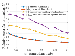
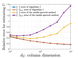
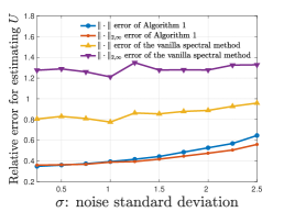
(a)	(b)	(c)

Figure 1: Relative estimation errors of the subspace estimate $\bm{U}$ for both Algorithm 1 and the vanilla spectral method. The results are reported for (a) relative error vs. sampling rate $p$ (where $d_{1}=100$, $d_{2}=1000$, $r=4$, $\sigma=1$), (b) relative error vs. column dimension $d_{2}$ (where $d_{1}=100$, $r=4$, $\sigma=1$, $p=\frac{2r\log\left(d_{1}+d_{2}\right)}{\sqrt{d_{1}d_{2}}}$), and (c) relative error vs. noise standard deviation $\sigma$ (where $d_{1}=100$, $d_{2}=1000$, $r=4$, $p=0.1$).

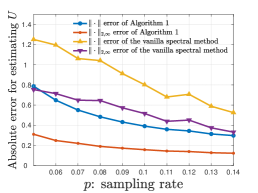
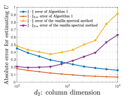
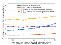
(a)	(b)	(c)

Figure 2: Absolute estimation errors of the subspace estimate $\bm{U}$ for both Algorithm 1 and the vanilla spectral method. The results are reported for (a) absolute error vs. sampling rate $p$ (where $d_{1}=100$, $d_{2}=1000$, $r=4$, $\sigma=1$), (b) absolute error vs. column dimension $d_{2}$ (where $d_{1}=100$, $r=4$, $\sigma=1$, $p=\frac{2r\log\left(d_{1}+d_{2}\right)}{\sqrt{d_{1}d_{2}}}$), and (c) absolute error vs. noise standard deviation $\sigma$ (where $d_{1}=100$, $d_{2}=1000$, $r=4$, $p=0.1$).

Tensor completion from noise data.

Next, we consider numerically the problem of tensor completion from noisy observations of its entries. Recall the notations in Section 4.1. We generate $\bm{W}^{\star}\in\mathbb{R}^{d\times r}$ with i.i.d. standard Gaussian entries, and generate $N_{i,j,k}\overset{\mathrm{i.i.d.}}{\sim}\mathcal{N}\left(0,\sigma^{2}\right)$ independently for each $\left(i,j,k\right)\in\left[d\right]^{3}$. Figure 3(a) and Figure 3(b) illustrate the relative estimation errors of the subspace estimate $\bm{U}$ vs. the sampling rate $p$ and noise standard deviation $\sigma$, respectively. Encouragingly, Figure 3 shows that Algorithm 2 accurately recovers the subspace spanned by the tensor factors of interest (with respect to both the spectral norm and the $\ell_{2,\infty}$ norm); in particular, it is capable of producing faithful subspace estimates even when the vanilla spectral method fails.

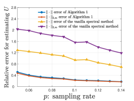
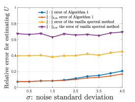
(a)	(b)

Figure 3: Relative estimation errors of the subspace $\bm{U}$ spanned by tensor components in tensor completion. The results are plotted for (a) relative error vs. sampling rate $p$ (where $d=100$, $r=4$, $\sigma=2$), and (b) relative error vs. noise standard deviation $\sigma$ (where $d=100$, $r=4$, $p=0.1$).

Covariance estimation with missing data.

The next series of experiments is concerned with covariance estimation with missing data. Recall the notations in Section 4.2. We draw $\bm{x}_{i}\overset{}{\sim}\mathcal{N}\left(\bm{{0}},\bm{\Sigma}^{\star}\right)$ independently with $\bm{\Sigma}^{\star}=\bm{U}^{\star}\bm{U}^{\star\top}$, where $\bm{U}^{\star}\in\mathbb{R}^{d\times r}$ is a i.i.d. standard Gaussian random matrix in $\mathbb{R}^{d\times r}$, and $\bm{\varepsilon}_{i}\overset{\mathrm{i.i.d.}}{\sim}\mathcal{N}\left(\bm{{0}},\sigma^{2}\bm{I}_{d}\right)$ for each $1\leq i\leq n$. We first consider the estimation error of the subspace. The numerical estimation errors of the estimate $\bm{U}$ vs. the sampling rate $p$, the sample size $n$ and the noise standard deviation $\sigma$ are plotted in Figure 4(a) – Figure 4(c), respectively. We then turn to the estimation accuracy of the covariance matrix. The numerical estimation errors of the estimate $\bm{S}$ of Algorithm 3 and the vanilla spectral method vs. the sampling rate $p$, the sample size $n$ and the noise standard deviation $\sigma$ are plotted in Figure 5, respectively. Similar to previous experiments, Algorithm 3 produces reliable estimates both in terms of the spectral norm, the $\ell_{2,\infty}$ norm and the $\ell_{\infty}$ norm accuracy.

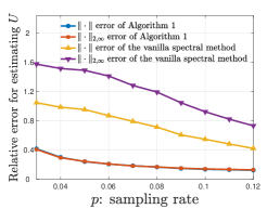
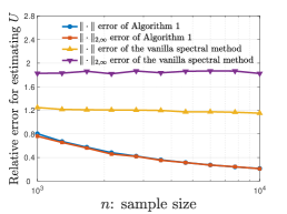
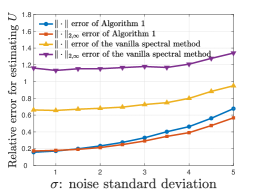
(a)	(b)	(c)

Figure 4: Relative error of the estimate $\bm{U}$ for covariance estimation with missing data. The results are shown for (a) relative error vs. sampling rate $p$ (where $d=100$, $n=5000$, $r=4$, $\sigma=1$), (b) relative error vs. sample size $n$ (where $d=100$, $r=4$, $\sigma=1$, $p=0.05$), and (c) relative error vs. noise standard deviation $\sigma$ (where $d=100$, $n=5000$, $r=4$, $p=0.1$).

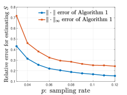
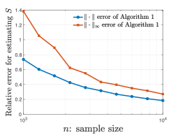
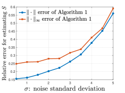
(a)	(b)	(c)
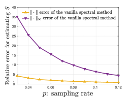
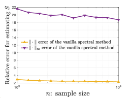
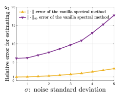
(d)	(e)	(f)

Figure 5: Relative error of the estimate $\bm{S}$ of Algorithm 3 (top row) and the vanilla spectral method (bottom row) for covariance estimation with missing data. The results are shown for (a,d) relative error vs. sampling rate $p$ (where $d=100$, $n=5000$, $r=4$, $\sigma=1$), (b,e) relative error vs. sample size $n$ (where $d=100$, $r=4$, $\sigma=1$, $p=0.05$), and (c,f) relative error vs. noise standard deviation $\sigma$ (where $d=100$, $n=5000$, $r=4$, $p=0.1$). It is worthnoting the different scales of the $y$-axis when plotting the errors of the two algorithms.

Community recovery in bipartite stochastic block model.

Finally, we conduct numerical experiments for community recovery in bipartite stochastic block models. The parameters are chosen to be $q_{\mathsf{in}}=\frac{a\log\left(n_{u}+n_{v}\right)}{\sqrt{n_{u}n_{v}}}$ and $q_{\mathsf{out}}=\frac{b\log\left(n_{u}+n_{v}\right)}{\sqrt{n_{u}n_{v}}}$ for some constants $a>b>0$. Figure 6(a) reveals a phase transition phenomenon concerned with exact community recovery. As can be seen, Algorithm 4 always succeeds in achieving exact recovery once $a$ — or equivalently $q_{\mathsf{in}}$ — exceeds a certain threshold, which outperforms the vanilla spectral method. In Figure 6(b), we vary the number $n_{v}$ nodes in $\mathcal{V}$ and plot the empirical success rates for exact recovery. The advantage of Algorithm 4 compared to the vanilla spectral method can be clearly seen from the plot.

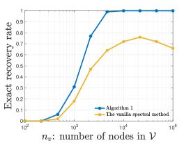
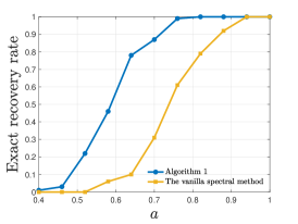
(a)	(b)

Figure 6: Empirical success rates for exact community recovery in bipartite stochastic block models, where $q_{\mathsf{in}}=\frac{a\log\left(n_{u}+n_{v}\right)}{\sqrt{n_{u}n_{v}}}$ and $q_{\mathsf{out}}=\frac{b\log\left(n_{u}+n_{v}\right)}{\sqrt{n_{u}n_{v}}}$. The results are shown for (a) empirical success rate vs. the number $n_{v}$ of nodes in $\mathcal{V}$ (where $n_{u}=100$, $a=0.8$, $b=0.01$), and (b) empirical exact recovery rate vs. $a$ (where $n_{u}=100$, $n_{v}=10000$, $b=0.01$).

5 Further related work

A natural class of spectral algorithms to estimate the leading singular subspace of a matrix — when given a noisy and sub-sampled copy of the true matrix — is to compute the leading left singular subspace of the observed data matrix. Despite the simplicity of this idea, this type of spectral methods provably achieves appealing performances for multiple statistical problems when the true matrix is (nearly) square. A partial list of examples includes low-rank matrix estimation and completion [KMO10a, JNS13, Cha15, CW15, MWCC17], community detection [RCY11, YP14, AFWZ17, Lei19], and synchronization and alignment [Sin11, AFWZ17, CC18a, SHSS16]. The $\ell_{2}$ statistical analysis of such algorithms relies heavily on the matrix perturbation theory such as the Davis-Kahan $\sin\bm{\Theta}$ theorem [DK70], the Wedin theorem [Wed72], and their extensions [Vu11, YWS14, OVW18, CZ18, CLC19, ZCW18].

However, the above-mentioned approach might lead to sub-optimal performance when the row dimension and the column dimension of the matrix differ dramatically. This issue has already been recognized in multiple contexts, including but not limited to unfolding-based spectral methods for tensor estimation [HSSS16, XY17, MS18, XZ19, ZX18] and spectral methods for biclustering [FP16]. Motivated by this sub-optimality issue, an alternative is to look at the “sample Gram matrix” which, as one expects, shares the same leading left singular space as the original observed data matrix. However, in the highly noisy or highly subsampled regime, the diagonal entries of the sample Gram matrix are highly biased, thus requiring special care. Several different treatments of diagonal components have been adopted for different contexts, including proper rescaling [MS18, Lou14, GRESS16], deletion [FP16], and iterative updates [ZCW18]. The deletion strategy is perhaps the simplest of this kind, as it does not require estimation of noise parameters. We note, however, that performing more careful iterative updates might be beneficial for certain heteroskedastic noise scenarios; see [ZCW18] for detailed discussions.

An important application of our work is the problem of tensor completion and estimation [GRY11, LMWY13, RPP13, KOKC13, MHWG14, RM14, GSSB17, SRK09, YZ16, YZ17, HZC18]. Despite its similarity to matrix completion, tensor completion is considerably more challenging; for concreteness and simplicity, we shall only discuss order-3 symmetric rank-$r$ tensors in $\mathbb{R}^{d^{3}}$. Motivated by the success of matrix completion, a simple strategy for tensor completion / denoising is to unfold the observed tensor into a $d\times d^{2}$ matrix and to apply standard matrix completion methods for completion. However, existing statistical guarantees derived in the matrix completion literature [CR09, KMO10a, Gro11] do not lead to useful bounds unless the sample size exceeds the order of $rd^{2}$, which far exceeds the requirement for other methods such as the sum-of-squares (SOS) hierarchy [BM16, PS17]. The work by [MS18] demonstrates that unfolding-based spectral algorithms can also lead to useful estimates under minimal sample complexity, as long as we look at the “Gram matrix” instead. In addition, such spectral algorithms also play an important role in initializing other nonconvex optimization methods [XY17, XYZ17, CLPC19, CPC20].

In addition, there is an enormous literature on covariance estimation and principal component analysis (PCA). For instance, the classical spiked covariance model [Joh01] has been extensively studied; in particular, the high-dimensional setting has inspired much investigation from both algorithmic and analysis perspectives [JL09, Pau07, BL08, Nad08, CY12, Ma13, CMW13, CMW15]. More recently, a computationally efficient algorithm called HeteroPCA has been proposed by [ZCW18] to achieve rate-optimal statistical guarantees for PCA in the presence of heteroskedastic noise. When it comes to incomplete data, a variety of methods have been introduced [Kie97, EvdG19, JH12]. For instance, Lounici considered estimating the top eigenvector in the setting of sparse PCA in [Lou13], and further proposed an estimator for the covariance matrix in [Lou14]. In [CZ16], bandable and sparse covariance matrices are considered. In addition, most of the prior work considered uniform random subsampling, and the recent work [ZWS19, PO19] began to account for heterogeneous missingness patterns.

Turning to the problem of community recovery or graph clustering, we note that extensive research has been carried out on stochastic block models or censored block models, which can be viewed as special cases of uni-partite networks [MNS14, Mas14, ABH15, MNS15, HWX16, CJSX14, CKST16, CRV15, GV16, CSG16, JMRT16, CLX18, CL15, GMZZ17]. The algorithms that enable exact community recovery in these block models include two-stage approaches [ABH15, MNS14] and semidefinite programming [HWX16, AL18, ABKK17, Ban18, GV16]. In addition, spectral clustering algorithms have been extensively studied as well [CO06, CO10, RCY11, YP14, LR15, YP16, AFWZ17, GMZZ17, Vu18, OVW18, STFP12, LMX15]. While this class of algorithms was originally developed to yield almost exact recovery (e.g. [ABH15]), the recent work by [AFWZ17, Lei19] uncovered that spectral methods alone are sufficient to achieve optimal exact community recovery (a.k.a. achieving strong consistency) for stochastic block models. The interested reader is referred to [Abb18] for an in-depth overview. Various extensions of the SBMs have been introduced and studied in the last few years. Our work contributes to this growing literature by justifying the optimality of spectral methods in bipartite stochastic block models [FPV15, FP16, GLMZ16].

Further, entrywise statistical analysis has recently received significant attention for various statistical problems [FWZ16, AFWZ17, MSC17, CFMW19, CCF18, ZB18, ASSS19, Lei19, EBW17, CTP19b, CTP19a, XZ19, RV15, PW19]. For instance, entrywise guarantees for spectral methods are obtained in [CCF18, EBW17] based on an algebraic Neumann trick, while the results in [ZB18, AFWZ17, CFMW19] were established based on a leave-one-out analysis. The work by [KL16, KX16, CCF18] went one step further by controlling an arbitrary linear form of the eigenvectors or singular vectors of interest. These results, however, typically lead to suboptimal performance guarantees when the row dimension and the column dimension of the matrix are substantially different.

Finally, we recently became aware of an unpublished work by Abbe, Fan and Wang [AFW19], which also considers statistical guarantees of PCA beyond the usual $\ell_{2}$ analysis; in particular, they develop an analysis framework that delivers tight $\ell_{p}$ perturbation bounds. Note, however, that their results are very different from the ones presented here. For instance, the results presented herein emphasize the scenarios with drastically different $d_{1}$ and $d_{2}$, which are not the main focus of [AFW19].

6 Analysis

In this section, we discuss in detail the analysis techniques employed to establish Theorem 1. This is built upon a leave-one-out (as well as a leave-two-out) analysis strategy that is particularly effective in controlling entrywise and $\ell_{2,\infty}$ estimation errors [EKBB⁺13, EK15, ZB18, CFMW19, AFWZ17, SCC17, CCFM19, CFMY19, CLL19, LBEK18, PW19].

6.1 Leave-one-out and leave-two-out estimates

In order to facilitate the analysis when bounding $\left\|\bm{U}\bm{R}-\bm{U}^{\star}\right\|_{2,\infty}$, we introduce a set of auxiliary leave-one-out matrices — a powerful analysis technique that has been employed to decouple complicated statistical dependency. It is worth emphasizing that these procedures are never executed in practice. Specifically, for each $1\leq m\leq d_{1}$, we introduce an auxiliary matrix

$$\bm{A}^{(m)} =\mathcal{P}_{-m,:}\left(\bm{A}\right)+p\mathcal{P}_{m,:}\left(\bm{A}^{\star}\right),$$ (44)

where $\mathcal{P}_{-m,:}$ (resp. $\mathcal{P}_{m,:}$) represents the projection onto the subspace of matrices supported on the index subset $\left\{\left[d_{1}\right]\setminus\left\{m\right\}\right\}\times\left[d_{2}\right]$ (resp. $\left\{m\right\}\times\left[d_{2}\right]$). In other words, $\bm{A}^{(m)}$ is obtained by replacing all entries in the $m$-th row by their expected values (taking into account the sampling rate). By construction, (1) $\bm{A}^{(m)}$ is statistically independent of the data in the $m$-th row of $\bm{A}$, and (2) $\bm{A}^{(m)}$ is expected to be quite close to $\bm{A}$, as we only discard a small fraction of data when constructing $\bm{A}^{(m)}$. These two observations taken together allow for optimal control of the estimation error in the $m$-th row of $\bm{U}$.

Armed with the leave-one-out matrices, we are ready to introduce auxiliary leave-one-out procedures for subspace estimation. Similar to the matrix $\bm{G}$ in Algorithm 1 (whose eigenspace serves as an estimate of the column space of $\bm{U}^{\star}$), we define an auxiliary matrix $\bm{G}^{\left(m\right)}\in\mathbb{R}^{d_{1}\times d_{1}}$ as follows:

$$\bm{G}^{\left(m\right)}=\mathcal{P}_{\mathsf{off}\text{-}\mathsf{diag}}\Big{(}\tfrac{1}{p^{2}}\bm{A}^{\left(m\right)}\bm{A}^{\left(m\right)\top}\Big{)},$$ (45)

where $\mathcal{P}_{\mathsf{off}\text{-}\mathsf{diag}}\left(\cdot\right)$ (as already defined in Section 2.2) extracts out all off-diagonal entries from a matrix. The auxiliary procedure, which is summarized in Algorithm 5, is very similar to Algorithm 1 except that it operates upon $\bm{G}^{(m)}$.

Algorithm 5 The $m$-th leave-one-out sequence

1:  Input: sampling set $\Omega$, observed entries $\{A_{i,j}\mid\left(i,j\right)\in\Omega\}$, true entries $\{A^{\star}_{m,j}\mid j\in\left[d_{2}\right]\}$, sampling rate $p$, rank $r$.

2:  Let $\bm{U}^{\left(m\right)}\bm{\Lambda}^{\left(m\right)}\bm{U}^{\left(m\right)\top}$ be the (truncated) rank-$r$ eigen-decomposition of $\bm{G}^{\left(m\right)}$. Here, $\bm{G}^{\left(m\right)}$ and $\bm{A}^{\left(m\right)}$ are defined respectively in (45) and (44).

3:  Output $\bm{U}^{\left(m\right)}$ as the subspace estimate and $\bm{\Sigma}^{\left(m\right)}={(\bm{\Lambda}^{\left(m\right)})}^{1/2}$ as the spectrum estimate.

Given that $\bm{A}^{(m)}$ (resp. $\bm{G}^{(m)}$) is very close to $\bm{A}$ (resp. $\bm{G}$), one would naturally expect $\bm{U}^{(m)}$ — the $r$-dimensional principal eigenspace of $\bm{G}^{(m)}$ — to stay extremely close to the original estimate $\bm{U}$. This fact will be formalized shortly.

As it turns out, given that the spectral method is applied to the Gram matrix (which is a quadratic form of the original data matrix), introducing the leave-one-out sequences alone is not yet sufficient for our purpose; we still need to introduce an additional set of “leave-two-out” matrices, in the hope of simultaneously handling the row-wise and the column-wise statistical dependency. Specifically, for each $1\leq m\leq d_{1}$ and each $1\leq l\leq d_{2}$, define the following auxiliary matrices:

$$\bm{A}^{\left(m,l\right)} :=\mathcal{P}_{-m,-l}\left(\bm{A}\right)+p\mathcal{\mathcal{P}}_{m,l}\left(\bm{A}^{\star}\right),$$ (46a)

$$\bm{G}^{\left(m,l\right)} :=\mathcal{P}_{\mathsf{off}\text{-}\mathsf{diag}}\left(\tfrac{1}{p^{2}}\bm{A}^{\left(m,l\right)}\bm{A}^{\left(m,l\right)\top}\right),$$ (46b)

where $\mathcal{\mathcal{P}}_{-m,-l}$ (resp. $\mathcal{\mathcal{P}}_{m,l}$) denotes the projection onto the subspace of matrices supported on $\left\{\left[d_{1}\right]\setminus\left\{m\right\}\right\}\times\left\{\left[d_{2}\right]\setminus\left\{l\right\}\right\}$ (resp. $\left\{m\right\}\times\left\{l\right\}$). Similar to $\bm{A}^{(m)}$, $\bm{A}^{(m,l)}$ is generated by replacing all data lying on the $m$-th row and the $l$-th column of $\bm{A}$ by their expected values (taking into account the sampling rate). The precise procedure is summarized in Algorithm 6. Similar to the leave-one-out estimates, one expects the new leave-two-out estimates $\bm{U}^{\left(m,l\right)}$ to be extremely close to $\bm{U}^{\left(m\right)}$ (and hence $\bm{U}$).

Algorithm 6 The $\left(m,l\right)$-th leave-two-out sequence

1:  Input: sampling set $\Omega$, observed entries $\{A_{i,j}\mid\left(i,j\right)\in\Omega\}$, true entries $\{A^{\star}_{m,j}\mid j\in\left[d_{2}\right]\}\cup\{A^{\star}_{i,l}\mid i\in\left[d_{1}\right]\}$, sampling rate $p$, rank $r$.

2:  Let $\bm{U}^{\left(m,l\right)}\bm{\Lambda}^{\left(m,l\right)}\bm{U}^{\left(m,l\right)\top}$ be the (truncated) rank-$r$ eigen-decomposition of $\bm{G}^{\left(m,l\right)}$. Here, $\bm{G}^{\left(m,l\right)}$ and $\bm{A}^{\left(m,l\right)}$ are defined respectively in (46b) and (46a).

3:  Output $\bm{U}^{\left(m,l\right)}$ as the subspace estimate and $\bm{\Sigma}^{\left(m,l\right)}={(\bm{\Lambda}^{\left(m,l\right)})}^{1/2}$ as the spectrum estimate.

6.2 Key lemmas

In this subsection, we provide several lemmas that play a crucial role in establishing our main theorem. These lemmas are primarily concerned with the proximity between the original estimate, the leave-one-out estimates, and the ground truth. Throughout this section, we let

$$\bm{G}^{\star}:=\bm{A}^{\star}\bm{A}^{\star\top}=\bm{U}^{\star}\bm{\Sigma}^{\star 2}\bm{U}^{\star\top}.$$ (47)

To begin with, we demonstrate that $\bm{G}$ is sufficiently close to $\bm{G}^{\star}$ when the difference is measured by the spectral norm. In view of standard matrix perturbation theory (which we shall make precise later), the proximity of $\bm{G}$ and $\bm{G}^{\star}$ is crucial in bounding the difference between $\bm{U}$ and $\bm{U}^{\star}$. The proof is deferred to Appendix B.2.

Lemma 1.

Instate the assumptions of Theorem 1. With probability at least $1-O\left(d^{-10}\right)$, one has

$$\left\|\bm{G}-\bm{G}^{\star}\right\| \lesssim\underset{=:\zeta_{\mathsf{op}}}{\underbrace{\frac{\mu r\sigma_{1}^{\star 2}\log d}{\sqrt{d_{1}d_{2}}\,p}+\sqrt{\frac{\mu r\sigma_{1}^{\star 4}\log d}{d_{2}p}}+\frac{\sigma^{2}\sqrt{d_{1}d_{2}}\,\log d}{p}+\sigma\sigma_{1}^{\star}\sqrt{\frac{d_{1}\log d}{p}}}}+\left\|\bm{A}^{\star}\right\|_{2,\infty}^{2}.$$ (48)

In order to get a better sense of the term $\zeta_{\mathsf{op}}$ appearing above, we make note of a straightforward yet useful fact, which reveals that $\zeta_{\mathsf{op}}$ is much smaller than any nonzero eigenvalue of $\bm{G}^{\star}$.

Fact 1.

Instate the assumptions of Theorem 1. Then the quantity $\zeta_{\mathsf{op}}$ as defined in (48) obeys

$$\zeta_{\mathsf{op}}+\left\|\bm{A}^{\star}\right\|_{2,\infty}^{2} \leq\frac{\mu r\sigma_{1}^{\star 2}\log d}{\sqrt{d_{1}d_{2}}\,p}+\sqrt{\frac{\mu r\sigma_{1}^{\star 4}\log d}{d_{2}p}}+\frac{\sigma^{2}}{\sigma_{r}^{\star 2}}\frac{\sqrt{d_{1}d_{2}}\,\log d}{p}+\sigma\sigma_{1}^{\star}\sqrt{\frac{d_{1}\log d}{p}}+\frac{\mu_{1}r\sigma_{1}^{\star 2}}{d_{1}}$$

$$\ll\frac{\sigma_{r}^{\star 2}}{\kappa^{2}},$$

where $\|\bm{A}^{\star}\|_{2,\infty}^{2}\leq\frac{\mu_{1}r\sigma_{1}^{\star 2}}{d_{1}}$ (cf. Lemma 11).

Further, the following lemma upper bounds the difference between $\bm{G}$ and $\bm{G}^{\star}$ in the $m$-th row, when projected onto the subspace represented by $\bm{U}^{\star}$; the proof is postponed to Appendix B.3. This result gives a more refined control of the difference between $\bm{G}$ and $\bm{G}^{\star}$.

Lemma 2.

Instate the assumptions of Theorem 1. With probability at least $1-O\left(d^{-10}\right)$, the following holds simultaneously for all $1\leq m\leq d_{1}$:

$$\big{\|}\left(\bm{G}-\bm{G}^{\star}\right)_{m,:}\bm{U}^{\star}\big{\|}_{2} \lesssim\big{(}\zeta_{\mathsf{op}}+\left\|\bm{A}^{\star}\right\|_{2,\infty}^{2}\big{)}\sqrt{\frac{\mu r}{d_{1}}},$$

where $\zeta_{\mathsf{op}}$ is defined in (48).

The next step, which is also the most challenging and crucial step, lies in showing that: every row of $\bm{U}$, under certain global linear transformation, serves as a good approximation of the corresponding row of $\bm{U}^{\star}$. Towards this end, we begin with the following preparations:

• We first introduce the following matrix $\bm{H}$ to represent the linear transformation we have in mind:

  $$\bm{H}:=\bm{U}^{\top}\bm{U}^{\star}.$$ (49)

  While this is not a rotation matrix, it is quite close to the rotation matrix $\bm{R}$ defined in (14).

• In addition, we find it convenient to express

  $$\bm{U}^{\star}=\bm{G}^{\star}\bm{U}^{\star}\left(\bm{\Sigma}^{\star}\right)^{-2}.$$

  Combining this with Lemma 2, one would expect $\bm{U}^{\star}$ and $\bm{G}\bm{U}^{\star}\left(\bm{\Sigma}^{\star}\right)^{-2}$ to be reasonably close, namely,

  $$\bm{U}^{\star}\approx\bm{G}\bm{U}^{\star}\left(\bm{\Sigma}^{\star}\right)^{-2}.$$ (50)

With these in hand, the following lemma (together with Lemma 2) asserts that

$$\bm{U}\bm{H}\approx\bm{G}\bm{U}^{\star}\left(\bm{\Sigma}^{\star}\right)^{-2}\approx\bm{U}^{\star}$$

in an $\ell_{2,\infty}$ sense.

Lemma 3.

Instate the assumptions of Theorem 1, and recall the definition of $\zeta_{\mathsf{op}}$ in (48). With probability at least $1-O(d^{-10})$, one has

$$\big{\|}\bm{U}\bm{H}-\bm{G}\bm{U}^{\star}\left(\bm{\Sigma}^{\star}\right)^{-2}\big{\|}_{2,\infty} \lesssim\frac{\kappa^{2}\big{(}\zeta_{\mathsf{op}}+\left\|\bm{A}^{\star}\right\|_{2,\infty}^{2}\big{)}}{\sigma_{r}^{\star 2}}\left(\left\|\bm{U}\bm{H}\right\|_{2,\infty}+\sqrt{\frac{\mu r}{d_{1}}}\right).$$

The proof of this lemma, however, goes far beyond conventional matrix perturbation theory, and requires delicate decoupling of statistical dependencies. This is accomplished via leave-one-out and leave-two-out analysis arguments. In what follows, we take a moment to explain the high-level idea.

To establish Lemma 3, we first learn from standard matrix perturbation theory[AFWZ17, Lemma 1] that: for each $1\leq m\leq d_{1}$,

$$\left\|\big{(}\bm{U}\bm{H}-\bm{G}\bm{U}^{\star}\left(\bm{\Sigma}^{\star}\right)^{-2}\big{)}_{m,:}\right\|_{2}\lesssim\frac{1}{\lambda_{r}\left(\bm{G}^{\star}\right)^{2}}\left\|\bm{G}-\bm{G}^{\star}\right\|\left\|\bm{G}_{m,:}\bm{U}^{\star}\right\|_{2}+\frac{1}{\lambda_{r}\left(\bm{G}^{\star}\right)}\left\|\bm{G}_{m,:}\left(\bm{U}\bm{H}-\bm{U}^{\star}\right)\right\|_{2}$$ (51)

holds, provided that $\bm{G}$ and $\bm{G}^{\star}$ are sufficiently close.

• The first term on the right-hand side of (51) can already be controlled by Lemma 1 and Lemma 2.

• The second term on the right-hand side of (51), however, is considerably more difficult to analyze, due to the complicated statistical dependence between $\bm{G}_{m,:}$ and $\bm{U\bm{H}}$. In order to decouple statistical dependency, we resort to the leave-one-out sequence $\bm{U}^{\left(m\right)}$ introduced in Algorithm 5 and use the triangle inequality to bound

  $$\left\|\bm{G}_{m,:}\left(\bm{U}\bm{H}-\bm{U}^{\star}\right)\right\|_{2}\leq\big{\|}\bm{G}_{m,:}\big{(}\bm{U}\bm{H}-\bm{U}^{\left(m\right)}\bm{H}^{\left(m\right)}\big{)}\big{\|}_{2}+\big{\|}\bm{G}_{m,:}\big{(}\bm{U}^{\left(m\right)}\bm{H}^{\left(m\right)}-\bm{U}^{\star}\big{)}\big{\|}_{2},$$ (52)

  where $\bm{H}^{(m)}:=\bm{U}^{(m)\top}\bm{U}^{\star}$. As mentioned before, the leave-one-out estimate $\bm{U}^{\left(m\right)}$ enjoys two nice properties.

  • The true estimate $\bm{U}$ and the leave-one-out estimate $\bm{U}^{(m)}$ are exceedingly close, as asserted by the following lemma (to be established in Appendix B.5).

    Lemma 4.

    Instate the assumptions of Theorem 1, and recall the definition of $\bm{H}$ in (49). With probability at least $1-O\left(d^{-10}\right)$, the following holds simultaneously for all $1\leq m\leq d_{1}$:

    $$\big{\|}\bm{U}^{\left(m\right)}\bm{U}^{\left(m\right)\top}-\bm{U}\bm{U}^{\top}\big{\|}_{\mathrm{F}} \lesssim\frac{\zeta_{\mathsf{op}}}{\sigma_{r}^{\star 2}}\left(\left\|\bm{U}\bm{H}\right\|_{2,\infty}+\sqrt{\frac{\mu r}{d_{1}}}\right),$$

    where $\zeta_{\mathsf{op}}$ is defined in (48).

    This result in turn allows us to control the first term on the right-hand side of (52).

  • Due to the statistical independence between $\bm{A}_{m,:}$ and $\bm{U}^{(m)}$, the matrices $\bm{G}_{m,:}$ and $\bm{U}^{(m)}$ turn out to be nearly independent. This allows one to invoke simple concentration inequalities to develop tight bounds for the second term on the right-hand side of (52). The detailed proof can be found in Appendix B.4.

Finally, we make a remark on a technical issue encountered in the proof of Lemma 4. Recall that $\bm{U}^{\left(m\right)}$ is obtained by simply replacing the $m$-th row of $\bm{A}$ with its population version, which indicates the statistical dependency between $\bm{U}^{\left(m\right)}$ and the $m$-th row of $\bm{A}$. However, there is still some delicate statistical dependency between $\bm{U}^{(m)}$ and the columns of $\bm{A}$ that need to be carefully coped with. Fortunately, the leave-two-out estimate $\bm{U}^{(m,l)}$ — which is obtained by dropping not only the $m$-th row of $\bm{A}$ but also the $l$-th of its columns — allows us to decouple the dependency between $\bm{U}^{(m,l)}$ (and hence $\bm{U}$ and $\bm{U}^{(m)}$) and the $l$-th column of $\bm{A}$. This is precisely the main reason why we introduce additional leave-two-out estimates.

6.3 Proof of Theorem 1

We are now positioned to establish our main theorem. The proof is split into two parts.

6.3.1 Statistical accuracy measured by $\left\|\cdot\right\|$

We begin by establishing the spectral norm bound (16c). Let $\lambda_{i}$ and $\lambda_{i}^{\star}$ be the $i$-th largest eigenvalue of $\bm{\Lambda}$ and $\bm{\Lambda^{\star}}$, respectively. From Lemma 1 and Weyl’s inequality, one finds that

$$\max_{1\leq i\leq r}\left|\lambda_{i}-\lambda_{i}^{\star}\right|=\left\|\bm{\Lambda}-\bm{\Lambda}^{\star}\right\| \leq\left\|\bm{G}-\bm{G}^{\star}\right\|\lesssim\zeta_{\mathsf{op}}+\|\bm{A}^{\star}\|_{2,\infty}^{2}\leq\sigma_{r}^{\star 2}\cdot\mathcal{E}_{\mathsf{general}},$$ (53)

where $\zeta_{\mathsf{op}}$ and $\mathcal{E}_{\mathsf{general}}$ are defined in (48) and (17), respectively. Here, the last inequality arises from the simple fact that $\|\bm{A}^{\star}\|_{2,\infty}^{2}\leq\frac{\mu_{1}r\sigma_{1}^{\star 2}}{d_{1}}$ (cf. Lemma 11). By virtue of Fact 1, we know that $\left\|\bm{\Lambda}-\bm{\Lambda}^{\star}\right\|\ll\sigma_{r}^{\star 2}$. Given that $\bm{\Lambda}^{\star}=\bm{\Sigma}^{\star 2}$ and $\bm{\Lambda}=\bm{\Sigma}^{2}$, this implies that for each $1\leq i\leq r$,

$$\frac{1}{4}\sigma_{i}^{\star 2}=\frac{1}{4}\lambda_{i}^{\star}\leq\lambda_{i}^{\star}-\left|\lambda_{i}-\lambda_{i}^{\star}\right|\leq\lambda_{i}\leq\lambda_{i}^{\star}+\left|\lambda_{i}-\lambda_{i}^{\star}\right|\leq 4\lambda_{i}^{\star}=4\sigma_{i}^{\star 2},$$

thus indicating that

$$\frac{1}{2}\sigma_{i}^{\star}\leq\sigma_{i}\leq 2\sigma_{i}^{\star}.$$ (54)

In conclusion,

$$\left\|\bm{\Sigma}-\bm{\Sigma}^{\star}\right\|=\max_{1\leq i\leq r}\left|\sigma_{i}-\sigma_{i}^{\star}\right|=\max_{1\leq i\leq r}\frac{\left|\sigma_{i}^{2}-\sigma_{i}^{\star 2}\right|}{\sigma_{i}+\sigma_{i}^{\star}}\overset{\mathrm{(a)}}{\leq}\max_{1\leq i\leq r}\frac{\left\|\bm{\Lambda}-\bm{\Lambda}^{\star}\right\|}{\frac{3}{2}\sigma_{i}^{\star}}\overset{\mathrm{(b)}}{\lesssim}\sigma_{r}^{\star}\cdot\mathcal{E}_{\mathsf{general}}$$

as claimed. Here, (a) comes from (54), whereas (b) follows from (53).

Next, we turn attention to (16a). First, it is seen that

$$\left\|\bm{U}\bm{R}-\bm{U}^{\star}\right\|\leq\sqrt{2}\left\|\bm{U}\bm{U}^{\top}-\bm{U}^{\star}\bm{U}^{\star\top}\right\|=\|\sin\bm{\Theta}(\bm{U},\bm{U}^{\star})\|$$ (55)

where $\bm{R}$ is defined in (14), and $\bm{\Theta}(\bm{U},\bm{U}^{\star})$ denotes a diagonal matrix whose $i$-th diagonal entry is the $i$-th principal angle between the two subspaces represented by $\bm{U}$ and $\bm{U}^{\star}$. Here, the first inequality follows from a well-known inequality connecting two different subspace distance metrics [SS90, Chapter II], while the last identity follows from [SS90, Chapter II]. In addition, Lemma 1 and Fact 1 tell us that

$$\left\|\bm{G}-\bm{G}^{\star}\right\| \lesssim\zeta_{\mathsf{op}}+\|\bm{A}^{\star}\|_{2,\infty}^{2}\ll\sigma_{r}^{\star 2}$$ (56)

with probability at least $1-O(d^{-10})$, which together with Weyl’s inequality gives

$$\lambda_{r+1}(\bm{G})\leq\lambda_{r+1}(\bm{G}^{\star})+\|\bm{G}-\bm{G}^{\star}\|=\|\bm{G}-\bm{G}^{\star}\|\leq\sigma_{r}^{\star 2}/2.$$ (57)

Therefore, [SS90, Chapter V, Theorem 3.6] (which is a version of the celebrated Davis-Kahan $\sin\bm{\Theta}$ Theorem[DK70]) reveals that

$$\|\sin\bm{\Theta}(\bm{U},\bm{U}^{\star})\| \leq\frac{\left\|\bm{G}-\bm{G}^{\star}\right\|}{\lambda_{r}\left(\bm{G}^{\star}\right)-\lambda_{r+1}\big{(}\bm{G}\big{)}}\leq\frac{\left\|\bm{G}-\bm{G}^{\star}\right\|}{\sigma_{r}^{\star 2}-\sigma_{r}^{\star 2}/2}=\frac{2\left\|\bm{G}-\bm{G}^{\star}\right\|}{\sigma_{r}^{\star 2}},$$

where we have used the fact $\lambda_{r}(\bm{G}^{\star})=\sigma_{r}^{\star 2}$. The above bounds taken collectively imply that, with probability at least $1-O(d^{-10})$,

$$\left\|\bm{U}\bm{R}-\bm{U}^{\star}\right\| \leq\frac{2\sqrt{2}\left\|\bm{G}-\bm{G}^{\star}\right\|}{\sigma_{r}^{\star 2}}\lesssim\mathcal{E}_{\mathsf{general}}.$$ (58)

6.3.2 Statistical accuracy measured by $\left\|\cdot\right\|_{2,\infty}$

Before continuing to the proof, we find it convenient to introduce a few more notations. In addition to the rotation matrix $\bm{R}$ defined in (14) and the linear transformation $\bm{H}$ defined in (49), we define

$$\mathsf{sgn}\left(\bm{H}\right) :=\widetilde{\bm{U}}\widetilde{\bm{V}}^{\top}\in\mathbb{R}^{d_{1}\times d_{1}},$$ (59)

where the columns of $\widetilde{\bm{U}}\in\mathbb{R}^{d_{1}\times d_{1}}$ (resp. $\widetilde{\bm{V}}\in\mathbb{R}^{d_{1}\times d_{1}}$) are the left (resp. right) singular vectors of $\bm{H}$. It is well-known that [TB77, Theorem 2]

$$\bm{R}=\mathsf{sgn}\left(\bm{H}\right).$$ (60)

We now move on to establishing the advertised bound (16b).

1. To begin with, we claim that $\bm{U}\bm{H}$ is extremely close to $\bm{U}\bm{R}$, provided that $\left\|\bm{G}-\bm{G}^{\star}\right\|$ is sufficiently small. To this end, recognizing that $\left\|\bm{G}-\bm{G}^{\star}\right\|\lesssim\zeta_{\mathsf{op}}\ll\sigma_{r}^{\star 2}$ (according to Lemma 1 and Fact 1), we can apply [AFWZ17, Lemma 3] to show that

   $$\left\|\bm{H}^{-1}\right\|\lesssim 1\qquad\text{and}\qquad\sqrt{\left\|\bm{H}-\mathsf{sgn}\left(\bm{H}\right)\right\|}\leq\left\|\bm{U}\bm{U}^{\top}-\bm{U}^{\star}\bm{U}^{\star\top}\right\|\lesssim\frac{\zeta_{\mathsf{op}}}{\sigma_{r}^{\star 2}},$$

   where the last inequality follows from (58). Thus, invoke the identity (60) to arrive at

   $$\left\|\bm{U}\bm{H}-\bm{U}\bm{R}\right\|_{2,\infty} =\left\|\bm{U}\bm{H}-\bm{U}\mathsf{sgn}\left(\bm{H}\right)\right\|_{2,\infty}=\left\|\bm{U}\bm{H}\bm{H}^{-1}\big{(}\bm{H}-\mathsf{sgn}\left(\bm{H}\right)\big{)}\right\|_{2,\infty}$$

   $$\leq\left\|\bm{U}\bm{H}\right\|_{2,\infty}\left\|\bm{H}^{-1}\right\|\left\|\bm{H}-\mathsf{sgn}\left(\bm{H}\right)\right\|$$

   $$\lesssim\left(\frac{\zeta_{\mathsf{op}}}{\sigma_{r}^{\star 2}}\right)^{2}\left\|\bm{U}\bm{H}\right\|_{2,\infty}\ll\frac{\zeta_{\mathsf{op}}}{\sigma_{r}^{\star 2}}\left\|\bm{U}\bm{H}\right\|_{2,\infty}.$$ (61)

   This in turn allows us to focus attention on bounding $\left\|\bm{U}\bm{H}-\bm{U}^{\star}\right\|_{2,\infty}$ (instead of $\left\|\bm{U}\bm{R}-\bm{U}^{\star}\right\|_{2,\infty}$).

2. Next, recall that $\bm{G}^{\star}=\bm{U}^{\star}\bm{\Sigma}^{\star 2}\bm{U}^{\star\top}$ and hence $\bm{G}^{\star}\bm{U}^{\star}(\bm{\Sigma}^{\star})^{-2}=\bm{U}^{\star}$. Invoke the triangle inequality to reach

   $$\left\|\bm{U}\bm{H}-\bm{U}^{\star}\right\|_{2,\infty} =\left\|\bm{U}\bm{H}-\bm{G}\bm{U}^{\star}\left(\bm{\Sigma}^{\star}\right)^{-2}+\bm{G}\bm{U}^{\star}\left(\bm{\Sigma}^{\star}\right)^{-2}-\bm{G}^{\star}\bm{U}^{\star}\left(\bm{\Sigma}^{\star}\right)^{-2}\right\|_{2,\infty}$$

   $$\leq\big{\|}\left(\bm{G}-\bm{G}^{\star}\right)\bm{U}^{\star}\left(\bm{\Sigma}^{\star}\right)^{-2}\big{\|}_{2,\infty}+\big{\|}\bm{U}\bm{H}-\bm{G}\bm{U}^{\star}\left(\bm{\Sigma}^{\star}\right)^{-2}\big{\|}_{2,\infty}$$

   $$\leq\left\|\left(\bm{G}-\bm{G}^{\star}\right)\bm{U}^{\star}\right\|_{2,\infty}\big{\|}\left(\bm{\Sigma}^{\star}\right)^{-2}\big{\|}+\big{\|}\bm{U}\bm{H}-\bm{G}\bm{U}^{\star}\left(\bm{\Sigma}^{\star}\right)^{-2}\big{\|}_{2,\infty}$$

   $$\leq\frac{1}{\sigma_{r}^{\star 2}}\left\|\left(\bm{G}-\bm{G}^{\star}\right)\bm{U}^{\star}\right\|_{2,\infty}+\big{\|}\bm{U}\bm{H}-\bm{G}\bm{U}^{\star}\left(\bm{\Sigma}^{\star}\right)^{-2}\big{\|}_{2,\infty}.$$ (62)

   Regarding the first term of (62), Lemma 2 reveals that with probability at least $1-O\left(d^{-10}\right)$,

   $$\frac{1}{\sigma_{r}^{\star 2}}\left\|\left(\bm{G}-\bm{G}^{\star}\right)\bm{U}^{\star}\right\|_{2,\infty} \lesssim\frac{\zeta_{\mathsf{op}}+\left\|\bm{A}^{\star}\right\|_{2,\infty}^{2}}{\sigma_{r}^{\star 2}}\sqrt{\frac{\mu r}{d_{1}}}.$$ (63)

   With regards to the second term of (62), Lemma 3 demonstrates that

   $$\big{\|}\bm{U}\bm{H}-\bm{G}\bm{U}^{\star}\left(\bm{\Sigma}^{\star}\right)^{-2}\big{\|}_{2,\infty}\lesssim \frac{\kappa^{2}\big{(}\zeta_{\mathsf{op}}+\left\|\bm{A}^{\star}\right\|_{2,\infty}^{2}\big{)}}{\sigma_{r}^{\star 2}}\left(\left\|\bm{U}\bm{H}\right\|_{2,\infty}+\sqrt{\frac{\mu r}{d_{1}}}\right)$$ (64)

   with probability at least $1-O\left(d^{-10}\right)$. Combine (63) and (64) to arrive at

   $$\left\|\bm{U}\bm{H}-\bm{U}^{\star}\right\|_{2,\infty} \lesssim\frac{\kappa^{2}\big{(}\zeta_{\mathsf{op}}+\left\|\bm{A}^{\star}\right\|_{2,\infty}^{2}\big{)}}{\sigma_{r}^{\star 2}}\left(\left\|\bm{U}\bm{H}\right\|_{2,\infty}+\sqrt{\frac{\mu r}{d_{1}}}\right).$$ (65)

3. As a byproduct of (65) and Fact 1, we see that

   $$\left\|\bm{U}\bm{H}-\bm{U}^{\star}\right\|_{2,\infty} \ll\left\|\bm{U}\bm{H}\right\|_{2,\infty}+\sqrt{\frac{\mu r}{d_{1}}}.$$

   It then follows from the triangle inequality that

   $$\left\|\bm{U}\bm{H}\right\|_{2,\infty}\leq\left\|\bm{U}\bm{H}-\bm{U}^{\star}\right\|_{2,\infty}+\left\|\bm{U}^{\star}\right\|_{2,\infty}\lesssim o\left(1\right)\left\|\bm{U}\bm{H}\right\|_{2,\infty}+\sqrt{\frac{\mu r}{d_{1}}},$$

   thus indicating that

   $$\left\|\bm{U}\bm{H}\right\|_{2,\infty}\leq 2\sqrt{\frac{\mu r}{d_{1}}}.$$ (66)

   Substitution into (61) and (65) gives

   $$\left\|\bm{U}\bm{H}-\bm{U}\bm{R}\right\|_{2,\infty}\ll\frac{\zeta_{\mathsf{op}}}{\sigma_{r}^{\star 2}}\sqrt{\frac{\mu r}{d_{1}}}\quad\text{and}\quad\left\|\bm{U}\bm{H}-\bm{U}^{\star}\right\|_{2,\infty}\lesssim\frac{\kappa^{2}\big{(}\zeta_{\mathsf{op}}+\left\|\bm{A}^{\star}\right\|_{2,\infty}^{2}\big{)}}{\sigma_{r}^{\star 2}}\sqrt{\frac{\mu r}{d_{1}}}.$$

Combining the above results yields

$$\left\|\bm{U}\bm{R}-\bm{U}^{\star}\right\|_{2,\infty} \leq\left\|\bm{U}\bm{H}-\bm{U}^{\star}\right\|_{2,\infty}+\left\|\bm{U}\bm{H}-\bm{U}\bm{R}\right\|_{2,\infty}$$

$$\lesssim\frac{\kappa^{2}\big{(}\zeta_{\mathsf{op}}+\left\|\bm{A}^{\star}\right\|_{2,\infty}^{2}\big{)}}{\sigma_{r}^{\star 2}}\sqrt{\frac{\mu r}{d_{1}}}.$$

Substituting the value of $\zeta_{\mathsf{op}}$ into the above inequality and using the upper bound $\|\bm{A}^{\star}\|_{2,\infty}^{2}\leq\frac{\mu_{1}r\sigma_{1}^{\star 2}}{d_{1}}$ (cf. Lemma 11), we conclude the proof.

7 Discussion

This paper has explored spectral methods tailored to subspace estimation for low-rank matrices with missing entries. In comparison to prior literature, our findings are particularly interesting when the column dimension $d_{2}$ far exceeds the row dimension $d_{1}$. In many scenarios, even though the observed data are either too noisy or too incomplete to support reliable recovery of the entire matrix (so that prior matrix completion results often become inapplicable), they might still be informative enough if the purpose is merely to estimate the column subspace of the unknown matrix. In fact, this suggests a potentially useful paradigm for privacy-preserving estimation or learning: the inability to recover the entire matrix facilitates the protection of personal data, yet it is still possible to retrieve useful subspace information for inference and learning. Our main contribution lies in establishing $\ell_{2,\infty}$ statistical guarantees for subspace estimation, therefore providing a stronger form of performance guarantees compared to the usual $\ell_{2}$ perturbation bounds.

Moving forward, there are many directions that are worth pursuing. For example, our current theory is likely suboptimal with respect to the dependence on the rank $r$ and the condition number $\kappa$. For instance, the conditions (15) and the risk bound (17) involve high-order polynomials of $\kappa$ in multiple places, and the rank $r$ in our current theory cannot exceed the order of $d_{1}/\kappa^{4}$; all of these might be improvable via more refined analysis. In addition, it is natural to wonder whether we can extend our algorithm and theory to accommodate more general sampling patterns. Going beyond estimation, an important direction lies in statistical inference and uncertainty quantification for subspace estimation, namely, how to construct valid and hopefully optimal confidence regions that are likely to contain the unknown column subspace? It would also be interesting to investigate how to incorporate other structural prior (e.g. sparsity) to further reduce the sample complexity and/or improve the estimation accuracy. Finally, another interesting avenue for future exploration is the extension to distributed or decentralized settings.

Appendix A Proofs for corollaries

A.1 Proof of Corollary 1

Recall that the spectral algorithm considered herein (cf. Section 4.1) operates upon the noisy copy of the mode-1 matricization of the tensor $\bm{T}^{\star}$, namely,

$$\bm{A}^{\star}=\sum_{s=1}^{r}\bm{w}_{s}^{\star}\left(\bm{w}_{s}^{\star}\otimes\bm{w}_{s}^{\star}\right)^{\top}.$$ (67)

Consequently, in order to apply Theorem 1, the main step boils down to estimating the spectrum and the incoherence parameters of $\bm{A}^{\star}$. Specifically, we need to upper bound the condition number $\kappa$, as well as the incoherence parameters $\mu_{0},\mu_{1}$ and $\mu_{2}$ as introduced in Definition 1.

Before proceeding, we introduce a few notations that simplify the presentation. Define

$$\lambda_{i}^{\star}:=\left\|\bm{w}_{i}^{\star}\right\|_{2}^{3},\qquad 1\leq i\leq r,$$

and let $\lambda_{\left(i\right)}^{\star}$ denote the $i$-th largest value in $\left\{\lambda_{i}^{\star}\right\}_{i=1}^{r}$. We also recall that

$$\lambda_{\min}^{\star}:=\min_{1\leq i\leq r}\left\|\bm{w}_{i}^{\star}\right\|_{2}^{3}\qquad\text{and}\qquad\lambda_{\max}^{\star}:=\max_{1\leq i\leq r}\left\|\bm{w}_{i}^{\star}\right\|_{2}^{3}.$$

In addition, we define two matrices of interest

$$\overline{\bm{W}}^{\star}:=\left[\overline{\bm{w}}_{1}^{\star},\cdots,\overline{\bm{w}}_{r}^{\star}\right]\in\mathbb{R}^{d\times r},\qquad\widetilde{\bm{W}}^{\star}:=\left[\overline{\bm{w}}_{1}^{\star}\otimes\overline{\bm{w}}_{1}^{\star},\cdots,\overline{\bm{w}}_{r}^{\star}\otimes\overline{\bm{w}}_{r}^{\star}\right]\in\mathbb{R}^{d^{2}\times r},$$

where $\overline{\bm{w}}_{s}^{\star}:=\bm{w}_{s}^{\star}/\left\|\bm{w}_{s}^{\star}\right\|_{2}$, and $\bm{a}\otimes\bm{b}:=\footnotesize\left[\begin{array}[]{c}a_{1}\bm{b}\\ \vdots\\ a_{d}\bm{b}\end{array}\right]$. In addition, let $\bm{D}^{\star}\in\mathbb{R}^{r\times r}$ be a diagonal matrix with diagonal entries

$$D_{s,s}^{\star}=\left\|\bm{w}_{s}^{\star}\right\|_{2},\qquad 1\leq s\leq r.$$

These allow us to express

$$\bm{G}^{\star}=\bm{A}^{\star}\bm{A}^{\star\top}=\overline{\bm{W}}^{\star}\bm{D}^{\star 3}\widetilde{\bm{W}}^{\star\top}\widetilde{\bm{W}}^{\star}\bm{D}^{\star 3}\overline{\bm{W}}^{\star\top}.$$

In the sequel, we begin by quantifying the spectrum of $\bm{G}^{\star}$, which in turn allows us to understand the spectrum of $\bm{A}^{\star}$.

• We first look at the eigenvalues of the matrices $\overline{\bm{W}}^{\star\top}\overline{\bm{W}}^{\star}$ and $\widetilde{\bm{W}}^{\star\top}\widetilde{\bm{W}}^{\star}$. Towards this, let us write

  $$\overline{\bm{W}}^{\star\top}\overline{\bm{W}}^{\star}=\bm{I}_{r}+\bm{C},\qquad\text{and}\qquad\widetilde{\bm{W}}^{\star\top}\widetilde{\bm{W}}^{\star}=\bm{I}_{r}+\widetilde{\bm{C}}$$ (68)

  for some matrices $\bm{C},\widetilde{\bm{C}}\in\mathbb{R}^{r\times r}$. It follows immediately from the incoherence assumption (27) that

  $$\left\|\bm{C}\right\|_{\infty}\leq\sqrt{\mu_{5}/d}\qquad\text{and}\qquad\big{\|}\widetilde{\bm{C}}\big{\|}_{\infty}\leq\mu_{5}/d,$$

  thus leading to the simple bounds

  $$\left\|\bm{C}\right\|\leq r\left\|\bm{C}\right\|_{\infty}\leq r\sqrt{\mu_{5}/d},\qquad\big{\|}\widetilde{\bm{C}}\big{\|}\leq r\,\big{\|}\widetilde{\bm{C}}\big{\|}_{\infty}\leq\mu_{5}r/d.$$ (69)

  These taken collectively with (68) and Weyl’s inequality yield

  $$\max_{i\in\left[r\right]}\Big{|}\lambda_{i}\big{(}\overline{\bm{W}}^{\star\top}\overline{\bm{W}}^{\star}\big{)}-1\Big{|}\leq\left\|\bm{C}\right\|\leq r\sqrt{\mu_{5}/d}\qquad\text{and}\qquad\max_{i\in\left[r\right]}\Big{|}\lambda_{i}\big{(}\widetilde{\bm{W}}^{\star\top}\widetilde{\bm{W}}^{\star}\big{)}-1\Big{|}\leq\big{\|}\widetilde{\bm{C}}\big{\|}\leq\mu_{5}r/d,$$

  which essentially tell us that

  $$\big{\|}\overline{\bm{W}}^{\star}\big{\|}=\sqrt{\lambda_{1}\big{(}\overline{\bm{W}}^{\star\top}\overline{\bm{W}}^{\star}\big{)}}\leq\sqrt{1+r\sqrt{\mu_{5}/d}}\qquad\text{and}\qquad\big{\|}\widetilde{\bm{W}}^{\star}\big{\|}=\sqrt{\lambda_{1}\big{(}\widetilde{\bm{W}}^{\star\top}\widetilde{\bm{W}}^{\star}\big{)}}\leq\sqrt{1+\mu_{5}r/d}.$$ (70)

• Returning to $\bm{G}^{\star}$, one invokes the definition (68) to deduce that

  $$\bm{G}^{\star}=\overline{\bm{W}}^{\star}\bm{D}^{\star 6}\overline{\bm{W}}^{\star\top}+\overline{\bm{W}}^{\star}\bm{D}^{\star 3}\widetilde{\bm{C}}\bm{D}^{\star 3}\overline{\bm{W}}^{\star\top}.$$

  Observe that the eigenvalues of $\overline{\bm{W}}^{\star}\bm{D}^{\star 3}\big{(}\overline{\bm{W}}^{\star}\bm{D}^{\star 3}\big{)}^{\top}$ are identical to those of $\big{(}\overline{\bm{W}}^{\star}\bm{D}^{\star 3}\big{)}^{\top}\overline{\bm{W}}^{\star}\bm{D}^{\star 3}$, where the latter can be further decomposed as follows (in view of (68))

  $$\big{(}\overline{\bm{W}}^{\star}\bm{D}^{\star 3}\big{)}^{\top}\overline{\bm{W}}^{\star}\bm{D}^{\star 3}=\bm{D}^{\star 3}\overline{\bm{W}}^{\star\top}\overline{\bm{W}}^{\star}\bm{D}^{\star 3}=\bm{D}^{\star 6}+\bm{D}^{\star 3}\bm{C}\bm{D}^{\star 3}.$$

  This taken together with Weyl’s inequality, (69) and (70) shows that

  $$\left|\lambda_{i}\big{(}\overline{\bm{W}}^{\star}\bm{D}^{\star 6}\overline{\bm{W}}^{\star\top}\big{)}-\lambda_{i}\big{(}\bm{D}^{\star 6}\big{)}\right|\leq\left\|\bm{D}^{\star 3}\bm{C}\bm{D}^{\star 3}\right\|\leq\left\|\bm{D}^{\star}\right\|^{6}\left\|\bm{C}\right\|\leq r\sqrt{\frac{\mu_{5}}{d}}\,\lambda_{\max}^{\star 2}$$

  for each $1\leq i\leq r$. In addition,

  $$\left|\lambda_{i}\big{(}\bm{G}^{\star}\big{)}-\lambda_{i}\big{(}\overline{\bm{W}}^{\star}\bm{D}^{\star 6}\overline{\bm{W}}^{\star\top}\big{)}\right|\leq\big{\|}\overline{\bm{W}}^{\star}\bm{D}^{\star 3}\widetilde{\bm{C}}\bm{D}^{\star 3}\overline{\bm{W}}^{\star\top}\big{\|}\leq\big{\|}\overline{\bm{W}}^{\star}\big{\|}^{2}\left\|\bm{D}^{\star}\right\|^{6}\big{\|}\widetilde{\bm{C}}\big{\|}\leq\frac{\mu_{5}r}{d}\left(1+r\sqrt{\frac{\mu_{5}}{d}}\right)\lambda_{\max}^{\star 2}.$$

  As a result, invoke the triangle inequality to see that

  $$\left|\lambda_{i}\left(\bm{G}^{\star}\right)-\lambda_{i}\left(\bm{D}^{\star 6}\right)\right| \leq\left|\lambda_{i}\big{(}\bm{G}^{\star}\big{)}-\lambda_{i}\big{(}\overline{\bm{W}}^{\star}\bm{D}^{\star 6}\overline{\bm{W}}^{\star\top}\big{)}\right|+\left|\lambda_{i}\big{(}\overline{\bm{W}}^{\star}\bm{D}^{\star 6}\overline{\bm{W}}^{\star\top}\big{)}-\lambda_{i}\big{(}\bm{D}^{\star 6}\big{)}\right|$$

  $$\leq\frac{\mu_{5}r}{d}\left(1+r\sqrt{\frac{\mu_{5}}{d}}\right)\lambda_{\max}^{\star 2}+r\sqrt{\frac{\mu_{5}}{d}}\,\lambda_{\max}^{\star 2}\leq 3r\sqrt{\frac{\mu_{5}}{d}}\,\lambda_{\max}^{\star 2}$$

  for each $1\leq i\leq r$, where the last inequality holds under the assumption that $r\sqrt{\mu_{5}/d}\leq 1$. This means

  $$\left|\lambda_{i}\left(\bm{G}^{\star}\right)-\lambda_{\left(i\right)}^{\star 2}\right| \leq 3r\sqrt{\frac{\mu_{5}}{d}}\,\lambda_{\max}^{\star 2},$$

  where $\lambda_{\left(i\right)}^{\star}$ denotes the $i$-th largest value in $\left\{\lambda_{i}^{\star}\right\}_{i=1}^{r}$.

• Recalling that $\mu_{\mathsf{tc}}:=\max\left\{\mu_{3},\mu_{4}^{2}\right\}$, $\kappa_{\mathsf{tc}}:=\lambda_{\max}^{\star}/\lambda_{\min}^{\star}$ and the rank assumption $r\ll\kappa_{\mathsf{tc}}^{-2}\sqrt{d/\mu_{5}}$, we find that

  $$\lambda_{i}\left(\bm{G}^{\star}\right)=\lambda_{\left(i\right)}^{\star 2}+O\left(r\sqrt{\frac{\mu_{5}}{d}}\right)\lambda_{\max}^{\star 2}\qquad\text{and}\qquad\sigma_{i}\left(\bm{A}^{\star}\right)=\lambda_{\left(i\right)}^{\star}\left(1+o\left(1\right)\right).$$ (71)

  As a result, we immediately arrive at

  $$\qquad\sigma_{1}\left(\bm{A}^{\star}\right)=\lambda_{\max}^{\star}\left(1+o\left(1\right)\right),\qquad\sigma_{r}\left(\bm{A}^{\star}\right)=\lambda_{\min}^{\star}\left(1+o\left(1\right)\right),\qquad\text{and}\qquad\kappa=\frac{\sigma_{1}\left(\bm{A}^{\star}\right)}{\sigma_{r}\left(\bm{A}^{\star}\right)}\lesssim\kappa_{\mathsf{tc}}.$$

Next, we turn attention to bounding the incoherence parameters of $\bm{A}^{\star}$. Let $\bm{A}^{\star}=\bm{U}^{\star}\bm{\Sigma}^{\star}\bm{V}^{\star\top}$ be the (compact) SVD of $\bm{A}^{\star}$. It is seen from (67) that the column space of $\bm{U}^{\star}$ (resp. $\bm{V}^{\star}$) coincides with the column space of $\overline{\bm{W}}^{\star}$ (resp. $\widetilde{\bm{W}}^{\star}$). Therefore, there exist orthonormal matrices $\bm{H}_{1}$ and $\bm{H}_{2}$ such that

$$\bm{U}^{\star}\bm{H}_{1}=\overline{\bm{W}}^{\star}\big{(}\overline{\bm{W}}^{\star\top}\overline{\bm{W}}^{\star}\big{)}^{-1/2}\qquad\text{and}\qquad\bm{V}^{\star}\bm{H}_{2}=\widetilde{\bm{W}}^{\star}\big{(}\widetilde{\bm{W}}^{\star\top}\widetilde{\bm{W}}^{\star}\big{)}^{-1/2}.$$

These allow us to bound

$$\left\|\bm{U}^{\star}\right\|_{2,\infty} =\left\|\bm{U}^{\star}\bm{H}_{1}\right\|_{2,\infty}\leq\big{\|}\overline{\bm{W}}^{\star}\big{\|}_{2,\infty}\big{\|}\big{(}\overline{\bm{W}}^{\star\top}\overline{\bm{W}}^{\star}\big{)}^{-1/2}\big{\|}\leq\sqrt{\frac{\mu_{4}r}{d}}\sqrt{\frac{1}{\lambda_{r}\big{(}\overline{\bm{W}}^{\star\top}\overline{\bm{W}}^{\star}\big{)}}}\lesssim\sqrt{\frac{\mu_{4}r}{d}}\sqrt{\frac{1}{1-1/3}}\leq\sqrt{\frac{2\mu_{4}r}{d}},$$

$$\left\|\bm{V}^{\star}\right\|_{2,\infty} =\left\|\bm{V}^{\star}\bm{H}_{2}\right\|_{2,\infty}\leq\big{\|}\widetilde{\bm{W}}^{\star}\big{\|}_{2,\infty}\big{\|}\big{(}\widetilde{\bm{W}}^{\star\top}\widetilde{\bm{W}}^{\star}\big{)}^{-1/2}\big{\|}\leq\sqrt{\frac{\mu_{4}^{2}r}{d^{2}}}\sqrt{\frac{1}{\lambda_{r}\big{(}\widetilde{\bm{W}}^{\star\top}\widetilde{\bm{W}}^{\star}\big{)}}}\leq\sqrt{\frac{\mu_{4}^{2}r}{d^{2}}}\sqrt{\frac{1}{1-1/3}}\leq\sqrt{\frac{2\mu_{4}^{2}r}{d^{2}}},$$

which follow from (70) and the assumption that $r\ll\sqrt{d/\mu_{5}}$. Moreover, the incoherence assumption (27) gives that

$$\mu_{0}=\frac{d^{3}\left\|\bm{A}^{\star}\right\|_{\infty}^{2}}{\left\|\bm{A}^{\star}\right\|_{\mathrm{F}}^{2}}=\frac{d^{3}\left\|\bm{T}^{\star}\right\|_{\infty}^{2}}{\left\|\bm{T}^{\star}\right\|_{\mathrm{F}}^{2}}\leq\mu_{3}.$$

To conclude, the above analysis reveals that

$$\mu_{0}\leq\mu_{3},\qquad\mu_{1}\lesssim\mu_{4},\qquad\mu_{2}\lesssim\mu_{4}^{2},\qquad\mu\lesssim\max\left\{\mu_{3},\mu_{4}^{2}\right\}=\mu_{\mathsf{tc}}\qquad\text{and}\qquad\kappa\lesssim\kappa_{\mathsf{tc}},$$

where $\mu=\max\left\{\mu_{0},\mu_{1},\mu_{2}\right\}$ and $\kappa=\sigma_{1}\left(\bm{A}^{\star}\right)/\sigma_{r}\left(\bm{A}^{\star}\right)$. With these estimates in place, Corollary 1 follows immediately from Theorem 1.

A.2 Proof of Corollary 2

In the problem of covariance estimation with missing data, the ground truth $\bm{A}^{\star}$ is effectively given by $\bm{B}^{\star}\bm{F}^{\star}$, which obeys

$$\bm{A}^{\star}=\bm{B}^{\star}\bm{F}^{\star}=\bm{U}^{\star}\bm{\Lambda}^{\star 1/2}\bm{F}^{\star}\in\mathbb{R}^{d\times n},\qquad\bm{F}^{\star}=\left[\bm{f}_{1}^{\star},\cdots,\bm{f}_{n}^{\star}\right]\in\mathbb{R}^{r\times n}$$

with $\bm{f}_{i}^{\star}\overset{\mathrm{i.i.d.}}{\sim}\mathcal{N}(\bm{0},\bm{I}_{r})$.We note that by our assumption on the sample size, one has $n\gg\kappa_{\mathsf{ce}}^{2}\left(r+\log d\right)$, where $\kappa_{\mathsf{ce}}=\lambda_{1}^{\star}/\lambda_{r}^{\star}$. In addition, we note that under the assumption of Corollary 2, one has

$$\mathcal{E}_{\mathsf{ce}}\ll\kappa_{\mathsf{ce}}^{-1}\leq 1,$$ (72)

where $\mathcal{E}_{\mathsf{ce}}$ and $\kappa_{\mathsf{ce}}$ are defined in (38) and (35), respectively.

A.2.1 Estimation error of the principle subspace

In this section, we will prove (37a) and (37b). To begin the proof, we verify the condition of the random noise (cf. (10)). From standard Gaussian concentration results, one is allowed to choose $R\asymp\sigma\sqrt{\log(n+d)}$, so that $|\eta_{i,j}|\leq R$ for all $i$ and $j$ with probability $1-O((n+d)^{-12})$. Under our sample size condition that $n\gg\max\big{\{}\frac{\log^{6}\left(n+d\right)}{dp^{2}},\frac{\log^{3}\left(n+d\right)}{p}\big{\}}$, the requirement (10) is satisfied, namely,

$$\frac{R^{2}}{\sigma^{2}}\asymp\log(n+d)\lesssim\min\left\{\frac{p\sqrt{dn}}{\log\left(n+d\right)},\frac{pn}{\log\left(n+d\right)}\right\}.$$

Next, we turn to the properties of $\bm{B}^{\star}\bm{F}^{\star}$ and start by looking at its spectrum. Define

$$\bm{C}:=\bm{F}^{\star}\bm{F}^{\star\top}-n\bm{I}_{r},$$

which allows us to write

$$\bm{G}^{\star}=\bm{B}^{\star}\bm{F}^{\star}\left(\bm{B}^{\star}\bm{F}^{\star}\right)^{\top}=\bm{U}^{\star}\bm{\Lambda}^{\star 1/2}\bm{F}^{\star}\bm{F}^{\star\top}\bm{\Lambda}^{\star 1/2}\bm{U}^{\star\top}=n\underbrace{\bm{U}^{\star}\bm{\Lambda}^{\star}\bm{U}^{\star\top}}_{=\bm{S}^{\star}}+\underbrace{\bm{U}^{\star}\bm{\Lambda}^{\star 1/2}\bm{C}\bm{\Lambda}^{\star 1/2}\bm{U}^{\star\top}}_{=:\,\bm{\Delta}}.$$ (73)

Using standard results on Gaussian random matrices [Ver12], one obtains

$$\left\|\bm{C}\right\| \lesssim\max\left\{\sqrt{n}\,\big{(}\sqrt{r}+\sqrt{\log\left(n+d\right)}\big{)},r+\log\left(n+d\right)\right\}\asymp\sqrt{n}\,\big{(}\sqrt{r}+\sqrt{\log\left(n+d\right)}\big{)},$$

$$\left|\sigma_{i}\left(\bm{F}^{\star}\right)-\sqrt{n}\right| \lesssim\sqrt{r}+\sqrt{\log\left(n+d\right)}$$ (74)

with probability at least $1-O\big{(}\left(n+d\right)^{-10}\big{)}$, provided that $n\gg r+\log(n+d)$. It then follows from Weyl’s inequality that

$$\left|\lambda_{i}\left(\bm{G}^{\star}\right)-\lambda_{i}\left(n\bm{S}^{\star}\right)\right|=\left|\lambda_{i}\left(\bm{G}^{\star}\right)-\lambda_{i}^{\star}n\right| \leq\big{\|}\bm{\Delta}\big{\|}\leq\left\|\bm{C}\right\|\left\|\bm{U}^{\star}\right\|^{2}\left\|\bm{\Lambda}^{\star}\right\|\lesssim\lambda_{1}^{\star}\sqrt{n}\,\big{(}\sqrt{r}+\sqrt{\log\left(n+d\right)}\big{)}.$$ (75)

Under the sample size assumption $n\gg\kappa_{\mathsf{ce}}^{2}\left(r+\log\left(n+d\right)\right)$, we conclude that

$$\lambda_{i}\left(\bm{G}^{\star}\right)=\lambda_{i}^{\star}n\left(1+o\left(1\right)\right)\qquad\text{and}\qquad\sigma_{i}\left(\bm{B}^{\star}\bm{F}^{\star}\right)=\sqrt{\lambda_{i}^{\star}n}\left(1+o\left(1\right)\right),$$ (76)

and hence

$$\kappa\left(\bm{G}^{\star}\right)=\frac{\lambda_{1}\left(\bm{G}^{\star}\right)}{\lambda_{r}\left(\bm{G}^{\star}\right)}\asymp\kappa_{\mathsf{ce}}\qquad\text{and}\qquad\kappa\left(\bm{B}^{\star}\bm{F}^{\star}\right)=\frac{\sigma_{1}\left(\bm{B}^{\star}\bm{F}^{\star}\right)}{\sigma_{r}\left(\bm{B}^{\star}\bm{F}^{\star}\right)}\asymp\sqrt{\kappa_{\mathsf{ce}}}.$$ (77)

Further, we look at the entrywise infinity norm of $\bm{B}^{\star}\bm{F}^{\star}$. From standard Gaussian concentration inequalities,

$$\left\|\bm{B}^{\star}\bm{F}^{\star}\right\|_{\infty} =\max\nolimits_{i,j}\left|\left\langle\big{(}\bm{U}^{\star}\bm{\Lambda}^{\star 1/2}\big{)}_{i,:},\bm{f}_{j}^{\star}\right\rangle\right|\lesssim\big{\|}\bm{U}^{\star}\bm{\Lambda}^{\star 1/2}\big{\|}_{2,\infty}\sqrt{\log\left(n+d\right)}$$

$$\leq\left\|\bm{U}^{\star}\right\|_{2,\infty}\left\|\bm{\Lambda}^{\star}\right\|^{1/2}\sqrt{\log\left(n+d\right)}\leq\sqrt{\frac{\lambda_{1}^{\star}\mu_{\mathsf{ce}}r\log\left(n+d\right)}{d}}$$

holds with probability at least $1-O\big{(}\left(n+d\right)^{-10}\big{)}$. Meanwhile, one has

$$\left\|\bm{B}^{\star}\bm{F}^{\star}\right\|_{\mathrm{F}}\geq\left\|\bm{B}^{\star}\right\|_{\mathrm{F}}\sigma_{r}(\bm{F}^{\star})=\big{\|}\bm{\Lambda}^{\star 1/2}\big{\|}_{\mathrm{F}}\sigma_{r}(\bm{F}^{\star})\gtrsim\sqrt{\lambda_{r}^{\star}rn}=\sqrt{\frac{1}{{\kappa_{\mathsf{ce}}}}\lambda_{1}^{\star}rn},$$

where the last step follows from (76) and (77). As a result,

$$\left\|\bm{B}^{\star}\bm{F}^{\star}\right\|_{\infty}\leq\sqrt{\frac{\mu_{\mathsf{ce}}\kappa_{\mathsf{ce}}\log(n+d)}{nd}}\left\|\bm{B}^{\star}\bm{F}^{\star}\right\|_{\mathrm{F}}$$ (78)

Recalling the definition of $\mu_{0}$ in (5), one obtains

$$\mu_{0}\lesssim\mu_{\mathsf{ce}}\kappa_{\mathsf{ce}}\log\left(n+d\right).$$ (79)

When it comes to the incoherence parameters $\mu_{1}$ and $\mu_{2}$ (cf. (6)), it can be easily verified that

$$\mu_{1}=\frac{d}{r}\left\|\bm{U}^{\star}\right\|_{2,\infty}^{2}=\mu_{\mathsf{ce}}.$$

In addition, recognizing the existence of an orthonormal matrix $\bm{H}_{2}$ such that $\bm{V}^{\star}\bm{H}_{2}=\bm{F}^{\star\top}(\bm{F}^{\star}\bm{F}^{\star\top})^{-1/2}$, we can bound

$$\left\|\bm{V}^{\star}\right\|_{2,\infty} =\left\|\bm{V}^{\star}\bm{H}_{2}\right\|_{2,\infty}\leq\left\|\bm{F}^{\star\top}\right\|_{2,\infty}\big{\|}\left(\bm{F}^{\star}\bm{F}^{\star\top}\right)^{-1/2}\big{\|}\overset{(\text{i})}{\leq}\frac{\sqrt{r}+\sqrt{\log\left(n+d\right)}}{\sigma_{r}\left(\bm{F}^{\star}\right)}$$

$$\overset{\left(\mathrm{ii}\right)}{\lesssim}\frac{\sqrt{r}+\sqrt{\log\left(n+d\right)}}{\sqrt{n}-\sqrt{r}-\sqrt{\log\left(n+d\right)}}\overset{\left(\mathrm{iii}\right)}{\lesssim}\frac{\sqrt{r\log\left(n+d\right)}}{\sqrt{n}},$$

where (i) follows from the standard Gaussian concentration result that $\big{|}\left\|\bm{F}^{\star\top}\right\|_{2,\infty}-\sqrt{r}\big{|}\lesssim\sqrt{\log\left(n+d\right)}$ with probability $1-O\big{(}\left(n+d\right)^{-20}\big{)}$, (ii) arises from (74), and (iii) holds true under our sample size assumption. Consequently, we obtain

$$\mu_{2}=\frac{n}{r}\left\|\bm{V}^{\star}\right\|_{2,\infty}^{2}\lesssim\log\left(n+d\right).$$

Thus far, we have shown that

$$\sigma_{r}^{\star}\asymp\sqrt{\lambda_{r}^{\star}n},\quad\mu_{0}\lesssim\mu_{\mathsf{ce}}\kappa_{\mathsf{ce}}\log\left(n+d\right),\quad\mu_{1}=\mu_{\mathsf{ce}},\quad\mu_{2}\lesssim\log\left(n+d\right),\quad\mu\lesssim\mu_{\mathsf{ce}}\kappa_{\mathsf{ce}}\log\left(n+d\right)\quad\text{and}\quad\kappa\asymp\sqrt{\kappa_{\mathsf{ce}}},$$

where $\sigma_{r}^{\star}=\sigma_{r}^{\star}\left(\bm{B}^{\star}\bm{F}^{\star}\right)$, $\mu=\max\left\{\mu_{0},\mu_{1},\mu_{2}\right\}$ and $\kappa=\kappa\left(\bm{B}^{\star}\bm{F}^{\star}\right)$. Under the sample size assumption (36) and the rank condition $r\ll\frac{d}{\mu_{\mathsf{ce}}\kappa_{\mathsf{ce}}^{2}}$, it is straightforward to verify the condition (15) is satisfied, i.e.

$$p \gg\max\left\{\frac{\mu_{\mathsf{ce}}\kappa_{\mathsf{ce}}^{3}r\log^{3}\left(n+d\right)}{\sqrt{dn}},\,\frac{\mu_{\mathsf{ce}}\kappa_{\mathsf{ce}}^{5}r\log^{3}\left(n+d\right)}{n}\right\}\gtrsim\max\left\{\frac{\mu\kappa^{4}r\log^{2}\left(n+d\right)}{\sqrt{dn}},\,\frac{\mu\kappa^{8}r\log^{2}\left(n+d\right)}{n}\right\},$$

$$\frac{\sigma}{\sigma_{r}^{\star}} \asymp\frac{\sigma}{\sqrt{\lambda_{r}^{\star}n}}\ll\min\left\{\frac{\sqrt{p}}{\sqrt{\kappa_{\mathsf{ce}}}\sqrt[4]{dn}\sqrt{\log\left(n+d\right)}},\,\sqrt{\frac{p}{\kappa_{\mathsf{ce}}^{3}d\log\left(n+d\right)}}\right\}\lesssim\min\left\{\frac{\sqrt{p}}{\kappa\sqrt[4]{d_{1}d_{2}}\,\sqrt{\log d}},\frac{1}{\kappa^{3}}\sqrt{\frac{p}{d_{1}\log d}}\right\},$$

$$r \ll\frac{d}{\mu_{\mathsf{ce}}\kappa_{\mathsf{ce}}^{2}}\asymp\frac{d}{\mu_{1}\kappa^{4}}.$$

Applying Theorem 1 immediately establishes the claims (37a) and (37b) in Corollary 2. Along the way, we have also established the following upper bound (see Lemma 1), which will be useful in the sequel:

$$\left\|\bm{G}-\bm{G}^{\star}\right\| \lesssim\lambda_{r}\left(\bm{G}^{\star}\right)\cdot\mathcal{E}_{\mathsf{ce}}\asymp\lambda_{r}^{\star}n\cdot\mathcal{E}_{\mathsf{ce}}.$$ (80)

Here, we recall that $\bm{G}=\frac{1}{p^{2}}\mathcal{P}_{\mathsf{off}\text{-}\mathsf{diag}}\left(\mathcal{P}_{\Omega}(\bm{X})\mathcal{P}_{\Omega}(\bm{X})^{\top}\right)$.

A.2.2 Estimation error of the covariance matrix

It remains to prove (37c) and (37d). Before proceeding, we first recall that $\bm{U}\bm{\Lambda}\bm{U}^{\top}$ is the top-$r$ eigendecomposition of $\bm{G}$,

$$\bm{\Sigma}=\bm{\Lambda}^{1/2},\quad\bm{B}=\frac{1}{\sqrt{n}}\bm{U}\bm{\Sigma},\quad\bm{B}^{\star}=\bm{U}^{\star}\bm{\Lambda}^{\star 1/2}\quad\text{and}\quad\bm{R}=\underset{\bm{Q}\in\mathcal{O}^{r\times r}}{\arg\min}\left\|\bm{U}\bm{Q}-\bm{U}^{\star}\right\|_{\mathrm{F}}.$$ (81)

Let us also define

$$\bm{K}:=\underset{\bm{Q}\in\mathcal{O}^{r\times r}}{\arg\min}\left\|\bm{B}\bm{Q}-\bm{B}^{\star}\right\|_{\mathrm{F}}.$$

It is well known that the minimizer $\bm{K}$ is given by [TB77]

$$\bm{K}=\mathsf{sgn}\left(\bm{B}^{\top}\bm{B}^{\star}\right),$$

where the $\mathsf{sgn}(\cdot)$ function is defined in (59). Since $\bm{K}$ is an orthonormal matrix, one can express

$$\bm{S}-\bm{S}^{\star}=\left(\bm{B}\bm{K}\right)\left(\bm{B}\bm{K}\right)^{\top}-\bm{B}^{\star}\bm{B}^{\star\top}=\left(\bm{B}\bm{K}-\bm{B}^{\star}\right)\left(\bm{B}\bm{K}\right)^{\top}+\bm{B}^{\star}\left(\bm{B}\bm{K}-\bm{B}^{\star}\right)^{\top}.$$ (82)

As a result, everything boils down to controlling $\left\|\bm{B}\bm{K}-\bm{B}^{\star}\right\|$ and $\left\|\bm{B}\bm{K}-\bm{B}^{\star}\right\|_{2,\infty}$. To this end, we use (81) to reach the following useful decomposition

$$\bm{BK}-\bm{B}^{\star}=\frac{1}{\sqrt{n}}\bm{U}\bm{\Lambda}^{1/2}\left(\bm{K}-\bm{R}\right)+\bm{U}\left(\frac{1}{\sqrt{n}}\bm{\Lambda}^{1/2}\bm{R}-\bm{R}\bm{\Lambda}^{\star 1/2}\right)+\left(\bm{U}\bm{R}-\bm{U}^{\star}\right)\bm{\Lambda}^{\star 1/2}.$$ (83)

Given that $\bm{U}\frac{1}{n}\bm{\Lambda}\bm{U}^{\top}$ is the top-$r$ eigendecomposition of $\frac{1}{n}\bm{G}$, an important step lies in controlling the difference between $\frac{1}{n}\bm{G}$ and $\bm{S}^{\star}$. Recalling the matrix $\bm{\Delta}$ as defined in (73), one can use (75), (80) as well as the definition of $\mathcal{E}_{\mathsf{ce}}$ (cf. (38)) to obtain

$$\left\|\frac{1}{n}\bm{G}-\bm{S}^{\star}\right\| \leq\frac{1}{n}\left\|\bm{G}-\bm{G}^{\star}\right\|+\left\|\frac{1}{n}\bm{G}^{\star}-\bm{S}^{\star}\right\|=\frac{1}{n}\left\|\bm{G}-\bm{G}^{\star}\right\|+\frac{1}{n}\left\|\bm{\Delta}\right\|$$

$$\lesssim\frac{1}{n}\lambda_{r}\left(\bm{G}^{\star}\right)\cdot\mathcal{E}_{\mathsf{ce}}+\frac{\lambda_{1}^{\star}}{\sqrt{n}}\big{(}\sqrt{r}+\sqrt{\log\left(n+d\right)}\big{)}\asymp\lambda_{r}^{\star}\cdot\mathcal{E}_{\mathsf{ce}},$$

where the last inequality makes use of the identity $\lambda_{r}(\bm{G}^{\star})\asymp n\lambda_{r}^{\star}$. Hence, apply [MWCC17, Lemma 46, Lemma 47] (with slight modification on $\kappa$) and Weyl’s inequality to show that

$$\left\|\frac{1}{\sqrt{n}}\bm{\Lambda}^{1/2}\bm{R}-\bm{R}\bm{\Lambda}^{\star 1/2}\right\| \lesssim\frac{\kappa\left(\bm{S}^{\star}\right)}{\sqrt{\lambda_{r}\left(\bm{S}^{\star}\right)}}\left\|\frac{1}{n}\bm{G}-\bm{S}^{\star}\right\|\lesssim\kappa_{\mathsf{ce}}\sqrt{\lambda_{r}^{\star}}\cdot\mathcal{E}_{\mathsf{ce}};$$ (84)

$$\left\|\bm{K}-\bm{R}\right\| \lesssim\frac{\sqrt{\kappa\left(\bm{S}^{\star}\right)}}{\lambda_{r}\left(\bm{S}^{\star}\right)}\left\|\frac{1}{n}\bm{G}-\bm{S}^{\star}\right\|\lesssim\sqrt{\kappa_{\mathsf{ce}}}\cdot\mathcal{E}_{\mathsf{ce}}.$$ (85)

In addition, it follows from Weyl’s inequality that

$$\left\|\frac{1}{n}\bm{\Lambda}-\bm{\Lambda}^{\star}\right\|\leq\left\|\frac{1}{n}\bm{G}-\bm{S}^{\star}\right\|\lesssim\lambda_{r}^{\star}\cdot\mathcal{E}_{\mathsf{ce}},$$

which combined with (72) gives

$$\frac{1}{n}\left\|\bm{\Lambda}\right\|\leq\left\|\frac{1}{n}\bm{\Lambda}-\bm{\Lambda}^{\star}\right\|+\left\|\bm{\Lambda}^{\star}\right\|\lesssim\lambda_{r}^{\star}\cdot\mathcal{E}_{\mathsf{ce}}+\lambda_{1}^{\star}\asymp\lambda_{1}^{\star}$$ (86)

under our assumptions.

We are ready to upper bound the difference between $\bm{BK}-\bm{B}^{\star}$. Plugging (37a), (84) (85) and (86) into (83) shows that

$$\left\|\bm{BK}-\bm{B}^{\star}\right\| \leq\frac{1}{\sqrt{n}}\left\|\bm{\Lambda}\right\|^{1/2}\left\|\bm{K}-\bm{R}\right\|+\left\|\frac{1}{\sqrt{n}}\bm{\Lambda}^{1/2}\bm{R}-\bm{R}\bm{\Lambda}^{\star 1/2}\right\|+\left\|\bm{U}\bm{R}-\bm{U}^{\star}\right\|\left\|\bm{\Lambda}^{\star}\right\|^{1/2}$$

$$\lesssim\sqrt{\kappa_{\mathsf{ce}}\lambda_{1}^{\star}}\cdot\mathcal{E}_{\mathsf{ce}}+\kappa_{\mathsf{ce}}\sqrt{\lambda_{r}^{\star}}\cdot\mathcal{E}_{\mathsf{ce}}+\sqrt{\lambda_{1}^{\star}}\cdot\mathcal{E}_{\mathsf{ce}}$$

$$\lesssim\kappa_{\mathsf{ce}}\sqrt{\lambda_{1}^{\star}}\cdot\mathcal{E}_{\mathsf{ce}}.$$ (87)

Since $\bm{K}\in\mathcal{O}^{r\times r}$, this also implies that

$$\left\|\bm{B}\right\|=\left\|\bm{BK}\right\|\leq\left\|\bm{BK}-\bm{B}^{\star}\right\|+\left\|\bm{B}^{\star}\right\|\lesssim\kappa_{\mathsf{ce}}\sqrt{\lambda_{1}^{\star}}\cdot\mathcal{E}_{\mathsf{ce}}+\sqrt{\lambda_{1}^{\star}}\asymp\sqrt{\lambda_{1}^{\star}},$$ (88)

where the last step results from (72). In addition, (37b), (72) and the fact that $\bm{R}\in\mathcal{O}^{r\times r}$ guarantees that

$$\left\|\bm{U}\right\|_{2,\infty}=\left\|\bm{U}\bm{R}\right\|_{2,\infty}\leq\left\|\bm{U}\bm{R}-\bm{U}^{\star}\right\|_{2,\infty}+\left\|\bm{U}^{\star}\right\|_{2,\infty}\lesssim\kappa_{\mathsf{ce}}^{3/2}\mathcal{E}_{\mathsf{ce}}\sqrt{\frac{\mu_{\mathsf{ce}}r\log\left(n+d\right)}{d}}+\sqrt{\frac{\mu_{\mathsf{ce}}r}{d}}\lesssim\sqrt{\frac{\kappa_{\mathsf{ce}}\mu_{\mathsf{ce}}r\log\left(n+d\right)}{d}}.$$

Consequently, it follows from the decomposition (83) that

$$\left\|\bm{BK}-\bm{B}^{\star}\right\|_{2,\infty} \leq\left\|\bm{U}\right\|_{2,\infty}\frac{1}{\sqrt{n}}\left\|\bm{\Lambda}\right\|^{1/2}\left\|\bm{K}-\bm{R}\right\|+\left\|\bm{U}\right\|_{2,\infty}\left\|\frac{1}{\sqrt{n}}\bm{\Lambda}^{1/2}\bm{R}-\bm{R}\bm{\Lambda}^{\star 1/2}\right\|+\left\|\bm{U}\bm{R}-\bm{U}^{\star}\right\|_{2,\infty}\left\|\bm{\Lambda}^{\star}\right\|^{1/2}$$

$$\lesssim\sqrt{\frac{\kappa_{\mathsf{ce}}^{2}\mu_{\mathsf{ce}}r\lambda_{1}^{\star}\log(n+d)}{d}}\,\mathcal{E}_{\mathsf{ce}}+\sqrt{\frac{\kappa_{\mathsf{ce}}^{3}\mu_{\mathsf{ce}}r\lambda_{r}^{\star}\log(n+d)}{d}}\,\mathcal{E}_{\mathsf{ce}}+\sqrt{\frac{\kappa_{\mathsf{ce}}^{3}\mu_{\mathsf{ce}}r\lambda_{1}^{\star}\log\left(n+d\right)}{d}}\,\mathcal{E}_{\mathsf{ce}}$$

$$\asymp\sqrt{\frac{\kappa_{\mathsf{ce}}^{3}\mu_{\mathsf{ce}}r\lambda_{1}^{\star}\log\left(n+d\right)}{d}}\,\mathcal{E}_{\mathsf{ce}}.$$ (89)

Combining (89) and (72) gives that

$$\left\|\bm{B}\right\|_{2,\infty} =\left\|\bm{BK}\right\|_{2,\infty}\leq\left\|\bm{BK}-\bm{B}^{\star}\right\|_{2,\infty}+\left\|\bm{B}^{\star}\right\|_{2,\infty}\lesssim\sqrt{\frac{\kappa_{\mathsf{ce}}^{3}\mu_{\mathsf{ce}}r\lambda_{1}^{\star}\log\left(n+d\right)}{d}}\,\mathcal{E}_{\mathsf{ce}}+\sqrt{\frac{\mu_{\mathsf{ce}}r\lambda_{1}^{\star}}{d}}$$

$$\lesssim\sqrt{\frac{\mu_{\mathsf{ce}}r\lambda_{1}^{\star}\log\left(n+d\right)}{d}},$$ (90)

where we use the fact that $\left\|\bm{B}^{\star}\right\|_{2,\infty}=\left\|\bm{U}^{\star}\bm{\Lambda}^{\star 1/2}\right\|_{2,\infty}\lesssim\left\|\bm{U}^{\star}\right\|_{2,\infty}\left\|\bm{\Lambda}^{\star}\right\|^{1/2}\lesssim\sqrt{\mu_{\mathsf{ce}}r\lambda_{1}^{\star}/d}$ and $\mathcal{E}_{\mathsf{ce}}\ll\kappa_{\mathsf{ce}}^{-1}$.

To finish up, we substitute (87) and (88) into (82) to find that

$$\left\|\bm{S}-\bm{S}^{\star}\right\| \leq\left\|\bm{B}\bm{K}-\bm{B}^{\star}\right\|\left(\left\|\bm{B}^{\star}\right\|+\left\|\bm{B}\bm{K}\right\|\right)\leq\left\|\bm{B}\bm{K}-\bm{B}^{\star}\right\|\left(\left\|\bm{B}^{\star}\right\|+\left\|\bm{B}\right\|\right)$$

$$\lesssim\kappa_{\mathsf{ce}}\lambda_{1}^{\star}\cdot\mathcal{E}_{\mathsf{ce}}.$$

Combining (89) and (90) reveals that

$$\left\|\bm{S}-\bm{S}^{\star}\right\|_{\infty} \leq\left\|\bm{B}\bm{K}-\bm{B}^{\star}\right\|_{2,\infty}\big{(}\left\|\bm{B}\bm{K}\right\|_{2,\infty}+\left\|\bm{B}^{\star}\right\|_{2,\infty}\big{)}\leq\left\|\bm{B}\bm{K}-\bm{B}^{\star}\right\|_{2,\infty}\big{(}\left\|\bm{B}\right\|_{2,\infty}+\left\|\bm{B}^{\star}\right\|_{2,\infty}\big{)}$$

$$\lesssim\frac{\kappa_{\mathsf{ce}}^{2}\mu_{\mathsf{ce}}r\lambda_{1}^{\star}\log\left(n+d\right)}{d}\cdot\mathcal{E}_{\mathsf{ce}}.$$

We have therefore established all claims.

A.3 Proof of Corollary 3

Recall from our calculation (42) that

$$\bm{A}^{\star}:=\mathbb{E}[\bm{A}]=\frac{\left(q_{\mathsf{in}}-q_{\mathsf{out}}\right)\sqrt{n_{u}n_{v}}}{2}\bm{u}^{\star}\bm{v}^{\star\top}$$

is a rank-1 matrix, where

$$\bm{u}^{\star}:=\frac{1}{\sqrt{n_{u}}}\left[\begin{array}[]{c}\bm{1}_{n_{u}/2}\\ -\bm{1}_{n_{u}/2}\end{array}\right]\qquad\text{and}\qquad\bm{v}^{\star}:=\frac{1}{\sqrt{n_{v}}}\left[\begin{array}[]{c}\bm{1}_{n_{v}/2}\\ -\bm{1}_{n_{v}/2}\end{array}\right].$$

Let $\bm{u}\in\mathbb{R}^{n_{u}}$ be the leading eigenvector of $\bm{G}$ (cf. (12) and Algorithm 4). To establish Corollary 3, the main step boils down to showing that, under the conditions of Corollary 3,

$$\min\left\{\left\|\bm{u}-\bm{u}^{\star}\right\|_{\infty},\left\|\bm{u}+\bm{u}^{\star}\right\|_{\infty}\right\} \lesssim\frac{1}{\sqrt{n_{u}}}\mathcal{E}_{{\mathsf{bsbm}}},$$ (91)

holds with probability exceeding $1-O\left(n^{-10}\right)$, where

$$\mathcal{E}_{{\mathsf{bsbm}}}:=\frac{q_{\mathsf{in}}}{\left(q_{\mathsf{in}}-q_{\mathsf{out}}\right)^{2}}\frac{\log n}{\sqrt{n_{u}n_{v}}}+\frac{\sqrt{q_{\mathsf{in}}}}{q_{\mathsf{in}}-q_{\mathsf{out}}}\sqrt{\frac{\log n}{n_{v}}}+\frac{1}{\sqrt{n_{u}}}.$$ (92)

If this claim (91) holds, then under our condition (43) one has $\mathcal{E}_{{\mathsf{bsbm}}}\ll 1$, and hence

$$\min\big{\{}\left\|\bm{u}-\bm{u}^{\star}\right\|_{\infty},\left\|\bm{u}+\bm{u}^{\star}\right\|_{\infty}\big{\}}\lesssim\frac{1}{\sqrt{n_{u}}}\mathcal{E}_{{\mathsf{bsbm}}}<\frac{1}{\sqrt{n_{u}}}.$$

In other words, one has either $\mathsf{sign}(u_{i})=\mathsf{sign}(u_{i}^{\star})$ for all $1\leq i\leq n_{u}$, or $\mathsf{sign}(u_{i})=-\mathsf{sign}(u_{i}^{\star})$ for all $1\leq i\leq n_{u}$. This tells us that the entrywise rounding operation applied to $\bm{u}$ is sufficient to recover exactly the community memberships of all nodes in $\mathcal{U}$.

The rest of the proof is devoted to establishing the claim (91). In order to apply Theorem 1, it suffices to estimate the spectrum and the incoherence parameters of $\bm{A}^{\star}$, as well as some simple statistical properties of $\bm{N}:=\bm{A}-\bm{A}^{\star}$.

• We begin by looking at $\bm{A}^{\star}$, which has rank 1 and satisfies

  $$\sigma_{1}\left(\bm{A}^{\star}\right)=\frac{\left(q_{\mathsf{in}}-q_{\mathsf{out}}\right)\sqrt{n_{u}n_{v}}}{2},\quad\left\|\bm{A}^{\star}\right\|_{\infty}=\frac{q_{\mathsf{in}}-q_{\mathsf{out}}}{2},\quad\left\|\bm{u}^{\star}\right\|_{\infty}=\frac{1}{\sqrt{n_{u}}},\quad\left\|\bm{v}^{\star}\right\|_{\infty}=\frac{1}{\sqrt{n_{v}}}.$$

  Recalling the definition of $\mu_{0},\mu_{1},\mu_{2}$ in (5) and (6), we obtain

  $$\mu_{0}=\frac{n_{u}n_{v}}{\left\|\bm{A}^{\star}\right\|_{\mathrm{F}}^{2}}\left\|\bm{A}^{\star}\right\|_{\infty}^{2}=1,\qquad\mu_{1}=n_{u}\left\|\bm{u}^{\star}\right\|_{2,\infty}^{2}=1,\qquad\mu_{2}=n_{v}\left\|\bm{v}^{\star}\right\|_{2,\infty}^{2}=1,\qquad\kappa=1.$$

• Next, we consider the maximum magnitude $R$ and the maximum variance $\sigma^{2}$ of all entries of $\bm{N}$ (see Assumption 2). Clearly, one has

  $$R =\text{$\max_{i,j}$}\left|N_{i,j}\right|\leq 1,$$

  $$\sigma^{2} =\max_{i,j}\mathbb{\mathsf{Var}}(N_{i,j})=\max\left\{q_{\mathsf{in}}(1-q_{\mathsf{in}}),q_{\mathsf{out}}(1-q_{\mathsf{out}})\right\}\leq\max\left\{q_{\mathsf{in}},q_{\mathsf{out}}\right\}\asymp q_{\mathsf{in}},$$

  which follows since $N_{i,j}$ is a centered Bernoulli random variable with parameter either $q_{\mathsf{in}}$ or $q_{\mathsf{out}}$. From the assumption (43) and the fact $q_{\mathsf{in}}^{2}\geq(q_{\mathsf{in}}-q_{\mathsf{out}})^{2}$, we know that

  $$q_{\mathsf{in}}\geq\frac{\left(q_{\mathsf{in}}-q_{\mathsf{out}}\right)^{2}}{q_{\mathsf{in}}}\gg\frac{\log n}{\sqrt{n_{u}n_{v}}}+\frac{\log n}{n_{v}}.$$

  Putting the above estimates together, we can straightforwardly verify the random noise requirement (10), namely,

  $$\frac{R^{2}}{\sigma^{2}}\lesssim\frac{1}{q_{\mathsf{in}}}\lesssim\frac{\min\left\{\sqrt{n_{u}n_{v}},n_{v}\right\}}{\log n}.$$

With the preceding bounds in place, Corollary 3 is an immediate consequence of Theorem 1.

Appendix B Proofs for key lemmas

This section aims to establish the key lemmas listed in Section 6.2.

B.1 Auxiliary quantities, notation, and preliminary facts

To simplify our treatment, the proofs shall consider the influence of missing data and that of noise altogether. Specifically, throughout this section, we shall define a rescaled version of $\bm{A}$ as follows

$$\bm{A}^{\mathsf{s}}:=\tfrac{1}{p}\bm{A}=\bm{A}^{\star}+\bm{E}\in\mathbb{R}^{d_{1}\times d_{2}},$$ (93)

where the matrix $\bm{E}$ represents the aggregate perturbation

$$\bm{E}:=\tfrac{1}{p}\mathcal{\mathcal{P}}_{\Omega}\left(\bm{A}^{\star}\right)-\bm{A}^{\star}+\tfrac{1}{p}\mathcal{\mathcal{P}}_{\Omega}\left(\bm{N}\right).$$ (94)

Clearly, $\bm{E}\in\mathbb{R}^{d_{1}\times d_{2}}$ is a random matrix with independent zero-mean entries and $\mathbb{E}\left[\bm{A}^{\mathsf{s}}\right]=\bm{A}^{\star}$. In addition, we define the corresponding leave-one-out and leave-two-out versions

$$\bm{A}^{\mathsf{s},\left(m\right)} :=\tfrac{1}{p}\bm{A}^{\left(m\right)},$$ (95)

$$\bm{A}^{\mathsf{s},\left(m,l\right)} :=\tfrac{1}{p}\bm{A}^{\left(m,l\right)},$$ (96)

for each $1\leq m\leq d_{1},1\leq l\leq d_{2}$.

As we shall see momentarily, it is convenient to introduce the following quantities regarding the above perturbation matrix $\bm{E}$: (1) $\max_{i\in\left[d_{1}\right],j\in\left[d_{2}\right]}\left|E_{i,j}\right|$; (2) $\max_{i\in\left[d_{1}\right],j\in\left[d_{2}\right]}\sqrt{\mathbb{E}\left[E_{i,j}^{2}\right]}$; (3) $\max_{i\in\left[d_{1}\right]}\sqrt{\sum_{j\in\left[d_{2}\right]}\mathbb{E}\left[E_{i,j}^{2}\right]}$; (4) $\max_{j\in\left[d_{2}\right]}\sqrt{\sum_{i\in\left[d_{1}\right]}\mathbb{E}\left[E_{i,j}^{2}\right]}$. In our settings, it is easy to verify — using the definition of incoherence parameters (cf. Definition 1), the assumptions of the random noise (cf. Assumption 2), and Lemma 11 — that the quantities defined above admit the following upper bounds

$$\max_{i\in\left[d_{1}\right],j\in\left[d_{2}\right]}\left|E_{i,j}\right| \leq\frac{\left\|\bm{A}^{\star}\right\|_{\infty}+R}{p}\lesssim\frac{\sqrt{\mu r}\,\sigma_{1}^{\star}}{\sqrt{d_{1}d_{2}}\,p}+\frac{\sigma\min\left\{\sqrt[4]{d_{1}d_{2}},\,\sqrt{d_{2}}\right\}}{\sqrt{p\log d}}=:B,$$ (97a)

$$\max_{i\in\left[d_{1}\right],j\in\left[d_{2}\right]}\sqrt{\mathbb{E}\left[E_{i,j}^{2}\right]} \leq\frac{\left\|\bm{A}^{\star}\right\|_{\infty}+\sigma}{\sqrt{p}}\leq\sigma_{1}^{\star}\sqrt{\frac{\mu r}{d_{1}d_{2}p}}+\frac{\sigma}{\sqrt{p}}=:\sigma_{\infty},$$ (97b)

$$\max_{i\in\left[d_{1}\right]}\sqrt{\sum_{j\in\left[d_{2}\right]}\mathbb{E}\left[E_{i,j}^{2}\right]} \leq\frac{\left\|\bm{A}^{\star}\right\|_{2,\infty}+\sigma\sqrt{d_{2}}}{\sqrt{p}}\leq\sigma_{1}^{\star}\sqrt{\frac{\mu r}{d_{1}p}}+\sigma\sqrt{\frac{d_{2}}{p}}=:\sigma_{\mathsf{row}},$$ (97c)

$$\max_{j\in\left[d_{2}\right]}\sqrt{\sum_{i\in\left[d_{1}\right]}\mathbb{E}\left[E_{i,j}^{2}\right]} \leq\frac{\left\|\bm{A}^{\star\top}\right\|_{2,\infty}+\sigma\sqrt{d_{1}}}{\sqrt{p}}\leq\sigma_{1}^{\star}\sqrt{\frac{\mu r}{d_{2}p}}+\sigma\sqrt{\frac{d_{1}}{p}}=:\sigma_{\mathsf{col}},$$ (97d)

with probability exceeding $1-O(d^{-12})$. Further, the following lemma singles out a few other useful properties about these quantities (to be established in Appendix B.6), which will be useful throughout the proof.

Lemma 5.

Instate the assumptions of Theorem 1. Then with probability at least $1-O\left(d^{-12}\right)$, we have

$$B \lesssim\frac{\min\left\{\sqrt{\sigma_{\mathsf{row}}\sigma_{\mathsf{col}}},\,\sigma_{\mathsf{row}}\right\}}{\sqrt{\log d}};$$ (98a)

$$\sigma_{\infty}^{2} \lesssim B\log d\left\|\bm{A}^{\star}\right\|\sqrt{\frac{\mu r}{d_{2}}}\lesssim\sigma_{\mathsf{col}}\sqrt{\log d}\left\|\bm{A}^{\star}\right\|\sqrt{\frac{\mu r}{d_{1}}};$$ (98b)

$$\sqrt{\frac{\mu r}{d_{1}}} \gtrsim\frac{B\log^{3/2}d\left\|\bm{A}^{\star}\right\|_{\infty}}{\left\|\bm{A}^{\star}\right\|^{2}};$$ (98c)

$$\sigma_{r}^{\star 2} \gg\max\Big{\{}\kappa^{2}\sigma_{\mathsf{col}}\sigma_{\mathsf{row}}\log d,\,\kappa^{2}\sigma_{\mathsf{col}}\sqrt{\log d}\left\|\bm{A}^{\star}\right\|,\,\kappa^{2}\left\|\bm{A}^{\star}\right\|_{2,\infty}^{2},\,\sigma_{\mathsf{row}}\sqrt{\frac{d_{1}\log d}{\mu r}}\left\|\bm{A}^{\star\top}\right\|_{2,\infty},\,B\log d\left\|\bm{A}^{\star}\right\|_{\infty}\Big{\}}.$$ (98d)

B.2 Proof of Lemma 1

The main component of the proof is to demonstrate that

$$\left\|\bm{G}-\bm{G}^{\star}\right\|\lesssim\underset{=:\delta_{\mathsf{op}}}{\underbrace{\left(\sigma_{\mathsf{row}}+\sigma_{\mathsf{col}}\right)\big{(}\sigma_{\mathsf{col}}+\left\|\bm{A}^{\star\top}\right\|_{2,\infty}\big{)}\log d+\sigma_{\mathsf{col}}\sqrt{\log d}\left\|\bm{A}^{\star}\right\|+\left\|\bm{A}^{\star}\right\|_{2,\infty}^{2}}}.$$ (99)

By substituting the values of $\sigma_{\mathsf{row}}$ and $\sigma_{\mathsf{col}}$ (cf. (97)) into the above expression, one derives

$$\delta_{\mathsf{op}}\lesssim\zeta_{\mathsf{op}}+\left\|\bm{A}^{\star}\right\|_{2,\infty}^{2},$$ (100)

where $\zeta_{\mathsf{op}}$ is defined in (48). Therefore, Lemma 1 is an immediate consequence of (99) and (100). The remainder of the proof amounts to justifying (99).

Recall the definitions of $\bm{G}$ and $\bm{G}^{\star}$ in (13) and (47), respectively. Given that $\bm{A}^{\mathsf{s}}=\bm{A}^{\star}+\bm{E}$, we can expand

$$\bm{G}-\bm{G}^{\star} =\mathcal{P}_{\mathsf{off}\text{-}\mathsf{diag}}\left(\bm{A}^{\mathsf{s}}\bm{A}^{\mathsf{s}\top}\right)-\bm{A}^{\star}\bm{A}^{\star\top}=\mathcal{P}_{\mathsf{off}\text{-}\mathsf{diag}}\left(\bm{A}^{\mathsf{s}}\bm{A}^{\mathsf{s}\top}-\bm{A}^{\star}\bm{A}^{\star\top}\right)-\mathcal{P}_{\mathsf{diag}}\left(\bm{A}^{\star}\bm{A}^{\star\top}\right)$$

$$=\mathcal{P}_{\mathsf{off}\text{-}\mathsf{diag}}\left(\bm{E}\bm{E}^{\top}\right)+\mathcal{P}_{\mathsf{off}\text{-}\mathsf{diag}}\left(\bm{A}^{\star}\bm{E}^{\top}+\bm{E}\bm{A}^{\star\top}\right)-\mathcal{P}_{\mathsf{diag}}\left(\bm{A}^{\star}\bm{A}^{\star\top}\right),$$ (101)

where $\mathcal{P}_{\mathsf{off}\text{-}\mathsf{diag}}$ and $\mathcal{P}_{\mathsf{diag}}$ are defined in Section 2.2. In what follows, we control these three terms separately.

B.2.1 Step 1: bounding the term $\mathcal{P}_{\mathsf{off}\text{-}\mathsf{diag}}\left(\bm{E}\bm{E}^{\top}\right)$

We first consider the term $\mathcal{P}_{\mathsf{off}\text{-}\mathsf{diag}}\left(\bm{E}\bm{E}^{\top}\right)$. Since $\left\{E_{i,j}\right\}_{i\in\left[d_{1}\right],j\in\left[d_{2}\right]}$ are independent zero-mean random variables, we can express

$$\mathcal{P}_{\mathsf{off}\text{-}\mathsf{diag}}\left(\bm{E}\bm{E}^{\top}\right)=\sum\nolimits_{1\leq l\leq d_{2}}\left(\bm{E}_{:,l}\bm{E}_{:,l}^{\top}-\bm{D}_{l}\right)$$ (102)

as a sum of independent zero-mean random matrices, where $\bm{D}_{l}$ is a random diagonal matrix in $\mathbb{R}^{d_{1}\times d_{1}}$ with entries

$$\big{(}\bm{D}_{l}\big{)}_{i,i}=E_{i,l}^{2}.$$ (103)

We intend to invoke the truncated matrix Bernstein inequality [HSSS16, Proposition A.7] to control the spectral norm of (102). To this end, we need to look at a few quantities.

• We first bound the spectral norm of the following covariance matrix

  $$\bm{\Sigma}_{\mathsf{ns}}:=\sum\nolimits_{1\leq l\leq d_{2}}\mathbb{E}\left[\left(\bm{E}_{:,l}\bm{E}_{:,l}^{\top}-\bm{D}_{l}\right)^{2}\right]\in\mathbb{R}^{d_{1}\times d_{1}}.$$

  Straightforward computation reveals that $\bm{\Sigma}_{\mathsf{ns}}$ is a diagonal matrix with entries

  $$\left(\bm{\Sigma}_{\mathsf{ns}}\right)_{i,i}=\sum\nolimits_{1\leq l\leq d_{2}}\mathbb{E}\left[E_{i,l}^{2}\right]\sum\nolimits_{m:m\neq i}\mathbb{E}\left[E_{m,l}^{2}\right]\leq\sigma_{\mathsf{row}}^{2}\sigma_{\mathsf{col}}^{2}$$

  for each $1\leq i\leq d_{1}$. This immediately reveals that

  $$V_{\mathsf{ns}}:=\left\|\bm{\Sigma}_{\mathsf{ns}}\right\|\leq\sigma_{\mathsf{row}}^{2}\sigma_{\mathsf{col}}^{2}.$$ (104)

• Next, we turn to upper bounding the spectral norm of each summand $\bm{E}_{:,l}\bm{E}_{:,l}^{\top}-\bm{D}_{l}$. As shown in the proof of Lemma 12, one has

  $$\mathbb{P}\left\{\left|\left\|\bm{E}_{:,l}\right\|_{2}^{2}-M_{1}\right|\geq t\right\} \leq 2\exp\left(-\frac{3}{8}\min\left\{\frac{t^{2}}{V_{1}},\frac{t}{L_{1}}\right\}\right),\quad t>0,$$

  where $M_{1},L_{1}$ and $V_{1}$ are given respectively by

  $$M_{1} :=\mathbb{E}\left[\left\|\bm{E}_{:,l}\right\|_{2}^{2}\right]\leq\sigma_{\mathsf{col}}^{2},$$

  $$L_{1} :=\max_{1\leq i\leq d_{1}}\left|E_{i,l}^{2}-\mathbb{E}\left[E_{i,l}^{2}\right]\right|\leq 2B^{2},$$

  $$V_{1} :=\sum\nolimits_{1\leq i\leq d_{1}}\mathsf{Var}\left(E_{i,l}^{2}\right)\leq B^{2}\sigma_{\mathsf{col}}^{2}.$$

  In addition, with probability exceeding $1-O\left(d^{-20}\right)$,

  $$\left\|\bm{E}_{:,l}\right\|_{2}^{2} \lesssim M_{1}+L_{1}\log d+\sqrt{V_{1}\log d}\lesssim\sigma_{\mathsf{col}}^{2}+B^{2}\log d+\sqrt{B^{2}\sigma_{\mathsf{col}}^{2}\log d}$$

  $$\asymp B^{2}\log d+\sigma_{\mathsf{col}}^{2},$$ (105)

  where the last line comes from the AM-GM inequality $2\sqrt{B^{2}\sigma_{\mathsf{col}}^{2}\log d}\leq B^{2}\log d+\sigma_{\mathsf{col}}^{2}$. This together with the definition $\bm{D}_{l}:=\mathsf{diag}\big{(}E_{i,l}^{2},\dots,E_{d_{1},l}^{2}\big{)}$ gives

  $$\left\|\bm{E}_{:,l}\bm{E}_{:,l}^{\top}-\bm{D}_{l}\right\|\leq\left\|\bm{E}_{:,l}\right\|_{2}^{2}+\left\|\bm{D}_{l}\right\|\leq 2\left\|\bm{E}_{:,l}\right\|_{2}^{2}\lesssim B^{2}\log d+\sigma_{\mathsf{col}}^{2}.$$

  Therefore, if we set

  $$L_{\mathsf{ns}}:=C\left(B^{2}\log d+\sigma_{\mathsf{col}}^{2}\right)$$ (106)

  for some sufficiently large constant $C>0$, then the above argument reveals that

  $$L_{\mathsf{ns}} \geq\frac{C}{3}\left(M_{1}+L_{1}\log d+\sqrt{V_{1}\log d}\right)\geq\frac{C}{3}\max\left\{\sqrt{V_{1}\log d},L_{1}\log d\right\}.$$

• In addition, one can easily bound that

  $$\mathbb{E}\left[\left\|\bm{E}_{:,l}\right\|_{2}^{2}\mathds{1}\left\{\left\|\bm{E}_{:,l}\right\|_{2}^{2}\geq L_{\mathsf{ns}}\right\}\right] \leq L_{\mathsf{ns}}\mathbb{P}\left\{\left\|\bm{E}_{:,l}\right\|_{2}^{2}\geq L_{\mathsf{ns}}\right\}+\int_{L_{\mathsf{ns}}}^{\infty}\mathbb{P}\left\{\left\|\bm{E}_{:,l}\right\|_{2}^{2}\geq t\right\}\mathrm{d}t$$

  $$\leq O\left(d^{-20}\right)L_{\mathsf{ns}}+\int_{L_{\mathsf{ns}}}^{\infty}\mathbb{P}\left\{\left\|\bm{E}_{:,l}\right\|_{2}^{2}\geq t\right\}\mathrm{d}t.$$

  Moreover, we know that $\min\big{\{}t^{2}/V_{1},t/L_{1}\big{\}}\geq t/\max\big{\{}\sqrt{V_{1}/\log d},L_{1}\big{\}}$ for any $t\geq L_{\mathsf{ns}}/2$. As a result, for sufficiently large $d$, we have

  $$\int_{L_{\mathsf{ns}}}^{\infty}\mathbb{P}\left\{\left\|\bm{E}_{:,l}\right\|_{2}^{2}\geq t\right\}\mathrm{d}t \leq\int_{L_{\mathsf{ns}}}^{\infty}\mathbb{P}\left\{\left|\left\|\bm{E}_{:,l}\right\|_{2}^{2}-M_{1}\right|>\frac{t}{2}\right\}\mathrm{d}t$$

  $$\leq 4\int_{\frac{1}{2}L_{\mathsf{ns}}}^{\infty}\exp\left(-\frac{3}{8}\min\left\{\frac{t^{2}}{V_{1}},\frac{t}{L_{1}}\right\}\right)\mathrm{d}t$$

  $$\leq 4\int_{\frac{1}{2}L_{\mathsf{ns}}}^{\infty}\exp\left(-\frac{3}{8}\frac{t}{\max\big{\{}\sqrt{V_{1}/\log d},L_{1}\big{\}}}\right)\mathrm{d}t$$

  $$\lesssim\max\big{\{}\sqrt{V_{1}/\log d},L_{1}\big{\}}\exp\left(-\frac{3}{16}\frac{L_{\mathsf{ns}}}{\max\big{\{}\sqrt{V_{1}/\log d},L_{1}\big{\}}}\right)$$

  $$\leq\max\big{\{}\sqrt{V_{1}/\log d},L_{1}\big{\}}\exp\left(-\frac{3C}{32}\log d\right)$$

  $$\ll\frac{L_{\mathsf{ns}}}{d^{2}},$$

  provided that $C>0$ is sufficiently large. Consequently, we have

  $$R_{\mathsf{ns}} :=\mathbb{E}\left[\left\|\bm{E}_{:,l}\bm{E}_{:,l}^{\top}-\bm{D}_{l}\right\|\mathds{1}\left\{\left\|\bm{E}_{:,l}\bm{E}_{:,l}^{\top}-\bm{D}_{l}\right\|\geq L_{\mathsf{ns}}\right\}\right]$$

  $$\leq\mathbb{E}\left[2\left\|\bm{E}_{:,l}\right\|_{2}^{2}\mathds{1}\left\{2\left\|\bm{E}_{:,l}\right\|_{2}^{2}\geq L_{\mathsf{ns}}\right\}\right]\ll\frac{L_{\mathsf{ns}}}{d^{2}}.$$ (107)

With estimates (104), (106) and (107) in place, we are ready to apply the truncated matrix Bernstein inequality [HSSS16, Proposition A.7] to obtain that, with probability at least $1-O\left(d^{-10}\right)$,

$$\left\|\mathcal{P}_{\mathsf{off}\text{-}\mathsf{diag}}\left(\bm{E}\bm{E}^{\top}\right)\right\| =\Big{\|}\sum\nolimits_{1\leq l\leq d_{2}}\bm{E}_{:,l}\bm{E}_{:,l}^{\top}-\bm{D}_{l}\Big{\|}\lesssim d_{2}R_{\mathsf{ns}}+L_{\mathsf{ns}}\log d+\sqrt{V_{\mathsf{ns}}\log d}$$

$$\asymp L_{\mathsf{ns}}\log d+\sqrt{V_{\mathsf{ns}}\log d}$$

$$\lesssim B^{2}\log^{2}d+\sigma_{\mathsf{col}}^{2}\log d+\sigma_{\mathsf{row}}\sigma_{\mathsf{col}}\sqrt{\log d}$$

$$\lesssim\sigma_{\mathsf{col}}\left(\sigma_{\mathsf{row}}+\sigma_{\mathsf{col}}\right)\log d,$$ (108)

where the last line results from the identity $B^{2}\log d\lesssim\sigma_{\mathsf{row}}\sigma_{\mathsf{col}}$ (See (98a)).

B.2.2 Step 2: bounding the term $\mathcal{P}_{\mathsf{off}\text{-}\mathsf{diag}}\left(\bm{A}^{\star}\bm{E}^{\top}+\bm{E}\bm{A}^{\star\top}\right)$

Next, we turn attention to $\mathcal{P}_{\mathsf{off}\text{-}\mathsf{diag}}\left(\bm{A}^{\star}\bm{E}^{\top}+\bm{E}\bm{A}^{\star\top}\right)$. By symmetry, it suffices to control to the spectral norm of $\mathcal{P}_{\mathsf{off}\text{-}\mathsf{diag}}\left(\bm{A}^{\star}\bm{E}^{\top}\right)$. To this end, we first express

$$\mathcal{P}_{\mathsf{off}\text{-}\mathsf{diag}}\left(\bm{A}^{\star}\bm{E}^{\top}\right)=\sum\nolimits_{1\leq l\leq d_{2}}\big{(}\bm{A}_{:,l}^{\star}\bm{E}_{:,l}^{\top}-\widehat{\bm{D}}_{l}\big{)}$$ (109)

as a sum of independent zero-mean random matrices, where $\widehat{\bm{D}}_{l}$ is a diagonal matrix obeying

$$\big{(}\widehat{\bm{D}}_{l}\big{)}_{i,i}=A_{i,l}^{\star}E_{i,l}.$$ (110)

To control (109), we need to first look at two matrices defined as follows

$$\widehat{\bm{\Sigma}}_{\mathsf{crs}} :=\sum\nolimits_{1\leq l\leq d_{2}}\mathbb{E}\Big{[}\big{(}\bm{A}_{:,l}^{\star}\bm{E}_{:,l}^{\top}-\widehat{\bm{D}}_{l}\big{)}\big{(}\bm{A}_{:,l}^{\star}\bm{E}_{:,l}^{\top}-\widehat{\bm{D}}_{l}\big{)}^{\top}\Big{]};$$

$$\widetilde{\bm{\Sigma}}_{\mathsf{crs}} :=\sum\nolimits_{1\leq l\leq d_{2}}\mathbb{E}\Big{[}\big{(}\bm{A}_{:,l}^{\star}\bm{E}_{:,l}^{\top}-\widehat{\bm{D}}_{l}\big{)}^{\top}\big{(}\bm{A}_{:,l}^{\star}\bm{E}_{:,l}^{\top}-\widehat{\bm{D}}_{l}\big{)}\Big{]}.$$

Straightforward computation shows that

$$\big{(}\widehat{\bm{\Sigma}}_{\mathsf{crs}}\big{)}_{i,i} =\sum\nolimits_{1\leq l\leq d_{2}}A_{i,l}^{\star 2}\mathbb{E}\left[\left\|\bm{E}_{:,l}\right\|_{2}^{2}-E_{i,l}^{2}\right],\quad\quad i\in\left[d_{1}\right],$$

$$\big{(}\widehat{\bm{\Sigma}}_{\mathsf{crs}}\big{)}_{i,j} =\sum\nolimits_{1\leq l\leq d_{2}}A_{i,l}^{\star}A_{j,l}^{\star}\mathbb{E}\left[\left\|\bm{E}_{:,l}\right\|_{2}^{2}-E_{i,l}^{2}-E_{j,l}^{2}\right],\quad\quad i\neq j,$$

and $\widetilde{\bm{\Sigma}}_{\mathsf{crs}}\in\mathbb{R}^{d_{1}\times d_{1}}$ is a diagonal matrix with entries

$$\big{(}\widetilde{\bm{\Sigma}}_{\mathsf{crs}}\big{)}_{i,i} =\sum\nolimits_{1\leq l\leq d_{2}}\left(\left\|\bm{A}_{:,l}^{\star}\right\|_{2}^{2}-A_{i,l}^{\star 2}\right)\mathbb{E}\left[E_{i,l}^{2}\right],\quad\quad i\in\left[d_{1}\right].$$

Hence we have

$$\big{\|}\widetilde{\bm{\Sigma}}_{\mathsf{crs}}\big{\|}\leq\max_{1\leq i\leq d_{1}}\big{|}\big{(}\widetilde{\bm{\Sigma}}_{\mathsf{crs}}\big{)}_{i,i}\big{|}\lesssim\sigma_{\mathsf{row}}^{2}\left\|\bm{A}^{\star\top}\right\|_{2,\infty}^{2}.$$ (111)

To control the spectral norm of $\widehat{\bm{\Sigma}}_{\mathsf{crs}}$, we further decompose it as $\widehat{\bm{\Sigma}}_{\mathsf{crs}}=\widehat{\bm{\Sigma}}_{\mathsf{crs}}^{{}^{\prime}}-\widehat{\bm{\Sigma}}_{\mathsf{crs}}^{{}^{\prime\prime}}$, where

$$\big{(}\widehat{\bm{\Sigma}}_{\mathsf{crs}}^{{}^{\prime}}\big{)}_{i,i} =\sum\nolimits_{1\leq l\leq d_{2}}A_{i,l}^{\star 2}\mathbb{E}\left[\left\|\bm{E}_{:,l}\right\|_{2}^{2}\right],\quad i\in\left[d_{1}\right],$$

$$\big{(}\widehat{\bm{\Sigma}}_{\mathsf{crs}}^{{}^{\prime}}\big{)}_{i,j} =\sum\nolimits_{1\leq l\leq d_{2}}A_{i,l}^{\star}A_{j,l}^{\star}\mathbb{E}\left[\left\|\bm{E}_{:,l}\right\|_{2}^{2}\right],\quad i\neq j,$$

and

$$\big{(}\widehat{\bm{\Sigma}}_{\mathsf{crs}}^{{}^{\prime\prime}}\big{)}_{i,i} =\sum\nolimits_{1\leq l\leq d_{2}}A_{i,l}^{\star 2}\mathbb{E}\left[E_{i,l}^{2}\right],\quad i\in\left[d_{1}\right],$$

$$\big{(}\widehat{\bm{\Sigma}}_{\mathsf{crs}}^{{}^{\prime\prime}}\big{)}_{i,j} =\sum\nolimits_{1\leq l\leq d_{2}}A_{i,l}^{\star}A_{j,l}^{\star}\mathbb{E}\left[E_{i,l}^{2}+E_{j,l}^{2}\right],\quad i\neq j.$$

• The spectral norm of $\widehat{\bm{\Sigma}}_{\mathsf{crs}}^{{}^{\prime}}$ can be easily upper bounded by

  $$\big{\|}\widehat{\bm{\Sigma}}_{\mathsf{crs}}^{{}^{\prime}}\big{\|} \leq\max_{1\leq l\leq d_{2}}\mathbb{E}\left[\left\|\bm{E}_{:,l}\right\|_{2}^{2}\right]\left\|\bm{A}^{\star}\bm{A}^{\star\top}\right\|\leq\sigma_{\mathsf{col}}^{2}\left\|\bm{A}^{\star}\right\|^{2}.$$ (112)

• Regarding $\widehat{\bm{\Sigma}}_{\mathsf{crs}}^{{}^{\prime\prime}}$, we first decompose $\widehat{\bm{\Sigma}}_{\mathsf{crs}}^{{}^{\prime\prime}}+\mathcal{P}_{\mathsf{diag}}\big{(}\widehat{\bm{\Sigma}}_{\mathsf{crs}}^{{}^{\prime\prime}}\big{)}=\bm{B}_{1}+\bm{B}_{2}$, where the diagonal entries of $\bm{B}_{1}$ and $\bm{B}_{2}$ are identical and equal to $\sum\nolimits_{1\leq l\leq d_{2}}A_{i,l}^{\star 2}\mathbb{E}\big{[}E_{i,l}^{2}\big{]},\left(1\leq i\leq d_{2}\right)$ while their off-diagonal parts are given by

  $$\left(\bm{B}_{1}\right)_{i,j}=\sum\nolimits_{1\leq l\leq d_{2}}A_{i,l}^{\star}\mathbb{E}\left[E_{i,l}^{2}\right]A_{j,l}^{\star}\qquad\text{and}\qquad\left(\bm{B}_{2}\right)_{i,j}=\sum\nolimits_{1\leq l\leq d_{2}}A_{i,l}^{\star}A_{j,l}^{\star}\mathbb{E}\left[E_{j,l}^{2}\right],\qquad i\neq j.$$

  Let $\bm{C}$ be a matrix in $\mathbb{R}^{d_{1}\times d_{2}}$ with entries $C_{i,j}=A_{i,j}^{\star}\mathbb{E}\left[E_{i,j}^{2}\right]$. One can easily check that $\bm{B}_{1}=\sum_{1\leq l\leq d_{2}}\bm{C}_{:,l}\bm{A}_{:,l}^{\star\top}=\bm{C}\bm{A}^{\star\top}$ and develop an upper bound

  $$\left\|\bm{B}_{1}\right\| \leq\left\|\bm{C}\right\|\left\|\bm{A}^{\star}\right\|\leq\left\|\bm{C}\right\|_{\mathrm{F}}\left\|\bm{A}^{\star}\right\|\leq\sigma_{\infty}^{2}\left\|\bm{A}^{\star}\right\|_{\mathrm{F}}\left\|\bm{A}^{\star}\right\|.$$

  Note that the same bound also holds for $\bm{B}_{2}$. Therefore, we arrive at

  $$\big{\|}\widehat{\bm{\Sigma}}_{\mathsf{crs}}^{{}^{\prime\prime}}\big{\|} \leq\big{\|}\mathcal{P}_{\mathsf{diag}}\big{(}\widehat{\bm{\Sigma}}_{\mathsf{crs}}^{{}^{\prime\prime}}\big{)}\big{\|}+\big{\|}\mathcal{P}_{\mathsf{diag}}\big{(}\widehat{\bm{\Sigma}}_{\mathsf{crs}}^{{}^{\prime\prime}}\big{)}+\widehat{\bm{\Sigma}}_{\mathsf{crs}}^{{}^{\prime\prime}}\big{\|}\leq\big{\|}\mathcal{P}_{\mathsf{diag}}\big{(}\widehat{\bm{\Sigma}}_{\mathsf{crs}}^{{}^{\prime\prime}}\big{)}\big{\|}+\left\|\bm{B}_{1}\right\|+\left\|\bm{B}_{2}\right\|$$

  $$\leq\sigma_{\infty}^{2}\left\|\bm{A}^{\star}\right\|_{2,\infty}^{2}+\sigma_{\infty}^{2}\left\|\bm{A}^{\star}\right\|_{\mathrm{F}}\left\|\bm{A}^{\star}\right\|$$

  $$\leq\sigma_{\infty}^{2}\left\|\bm{A}^{\star}\right\|_{2,\infty}^{2}+\sigma_{\infty}^{2}\sqrt{r}\left\|\bm{A}^{\star}\right\|^{2}$$

  $$\leq 2\sigma_{\infty}^{2}\sqrt{r}\left\|\bm{A}^{\star}\right\|^{2},$$

  where we have used the facts that $\left\|\bm{A}^{\star}\right\|_{2,\infty}\leq\left\|\bm{A}^{\star}\right\|$ and $\left\|\bm{A}^{\star}\right\|_{\mathrm{F}}\leq\sqrt{r}\left\|\bm{A}^{\star}\right\|$. Consequently, the above bounds taken collectively yield

  $$\big{\|}\widehat{\bm{\Sigma}}_{\mathsf{crs}}\big{\|}\leq\big{\|}\widehat{\bm{\Sigma}}_{\mathsf{crs}}^{{}^{\prime}}\big{\|}+\big{\|}\widehat{\bm{\Sigma}}_{\mathsf{crs}}^{{}^{\prime\prime}}\big{\|}\lesssim\left(\sigma_{\mathsf{col}}^{2}+\sigma_{\infty}^{2}\sqrt{r}\right)\left\|\bm{A}^{\star}\right\|^{2}\asymp\sigma_{\mathsf{col}}^{2}\left\|\bm{A}^{\star}\right\|^{2},$$ (113)

  where the last step uses (97b) and (97d).

Putting (111), (112) and (113) together yields

$$V_{\mathsf{crs}} :=\max\left\{\big{\|}\widehat{\bm{\Sigma}}_{\mathsf{crs}}\big{\|},\big{\|}\widetilde{\bm{\Sigma}}_{\mathsf{crs}}\big{\|}\right\}\lesssim\sigma_{\mathsf{col}}^{2}\left\|\bm{A}^{\star}\right\|^{2}+\sigma_{\mathsf{row}}^{2}\left\|\bm{A}^{\star\top}\right\|_{2,\infty}^{2}.$$ (114)

Second, we turn to the spectral norm of each summand $\bm{A}_{:,l}^{\star}\bm{E}_{:,l}^{\top}-\widehat{\bm{D}}_{l}$. Recalling the definition that $\widehat{\bm{D}}_{l}=\mathsf{diag}\big{(}A_{1,l}^{\star}E_{1,l},\dots,A_{d_{1},l}^{\star}E_{d_{1},l}\big{)}$, we can obtain

$$\big{\|}\bm{A}_{:,l}^{\star}\bm{E}_{:,l}^{\top}-\widehat{\bm{D}}_{l}\big{\|}\leq\left\|\bm{A}_{:,l}^{\star}\right\|_{2}\left\|\bm{E}_{:,l}\right\|_{2}+\big{\|}\widehat{\bm{D}}_{l}\big{\|}\leq 2\left\|\bm{A}_{:,l}^{\star}\right\|_{2}\left\|\bm{E}_{:,l}\right\|_{2}\leq 2\left\|\bm{A}^{\star\top}\right\|_{2,\infty}\left\|\bm{E}_{:,l}\right\|_{2}.$$

Set

$$L_{\mathsf{crs}} :=C\sqrt{L_{\mathsf{ns}}}\left\|\bm{A}^{\star\top}\right\|_{2,\infty}\asymp\big{(}\sigma_{\mathsf{col}}+B\sqrt{\log d}\big{)}\left\|\bm{A}^{\star\top}\right\|_{2,\infty},$$ (115)

where $L_{\mathsf{ns}}$ is defined in (106) and $C>0$ is some sufficiently large universal constant. Then with probability at least $1-O\left(d^{-20}\right)$, one has

$$\big{\|}\bm{A}_{:,l}^{\star}\bm{E}_{:,l}^{\top}-\widehat{\bm{D}}_{l}\big{\|} \leq 2\left\|\bm{A}^{\star\top}\right\|_{2,\infty}\left\|\bm{E}_{:,l}\right\|_{2}\lesssim L_{\mathsf{crs}},$$

where the last inequality comes from (105).

Third, we need to control

$$R_{\mathsf{crs}}:=\mathbb{E}\left[\big{\|}\bm{A}_{:,l}^{\star}\bm{E}_{:,l}^{\top}-\widehat{\bm{D}}_{l}\big{\|}\,\mathds{1}\big{\{}\big{\|}\bm{A}_{:,l}^{\star}\bm{E}_{:,l}^{\top}-\widehat{\bm{D}}_{l}\big{\|}\geq L_{\mathsf{crs}}\big{\}}\right].$$

From Jensen’s inequality and (107), we know that

$$\mathbb{E}\left[\left\|\bm{E}_{:,l}\right\|_{2}\mathds{1}\big{\{}\left\|\bm{E}_{:,l}\right\|_{2}\geq\sqrt{L_{\mathsf{ns}}}\big{\}}\right] \leq\sqrt{\mathbb{E}\left[\left\|\bm{E}_{:,l}\right\|_{2}^{2}\mathds{1}\big{\{}\left\|\bm{E}_{:,l}\right\|_{2}^{2}\geq L_{\mathsf{ns}}\big{\}}\right]}\ll\frac{\sqrt{L_{\mathsf{ns}}}}{d}.$$

By the definition of $L_{\mathsf{crs}}$ in (115) and the fact that

$$\left\{\left\|\bm{A}_{:,l}^{\star}\right\|_{2}\left\|\bm{E}_{:,l}\right\|_{2}\geq L_{\mathsf{crs}}\right\} \subset\left\{\left\|\bm{A}^{\star\top}\right\|_{2,\infty}\left\|\bm{E}_{:,l}\right\|_{2}\geq L_{\mathsf{crs}}\right\}=\left\{\left\|\bm{E}_{:,l}\right\|_{2}\geq C\sqrt{L_{\mathsf{ns}}}\right\},$$

one has

$$R_{\mathsf{crs}} \leq\mathbb{E}\left[2\left\|\bm{A}_{:,l}^{\star}\right\|_{2}\left\|\bm{E}_{:,l}\right\|_{2}\mathds{1}\big{\{}2\left\|\bm{A}_{:,l}^{\star}\right\|_{2}\left\|\bm{E}_{:,l}\right\|_{2}\geq L_{\mathsf{crs}}\big{\}}\right]$$

$$\lesssim\left\|\bm{A}^{\star\top}\right\|_{2,\infty}\mathbb{E}\Big{[}\left\|\bm{E}_{:,l}\right\|_{2}\mathds{1}\big{\{}\left\|\bm{E}_{:,l}\right\|_{2}\geq\frac{C}{2}\sqrt{L_{\mathsf{ns}}}\big{\}}\Big{]}$$

$$\ll\frac{1}{d}\left\|\bm{A}^{\star\top}\right\|_{2,\infty}\sqrt{L_{\mathsf{ns}}}\asymp\frac{L_{\mathsf{crs}}}{d}.$$ (116)

With (114), (115) and (116) in place, we can apply the truncated matrix Bernstein inequality to obtain that, with with probability at least $1-O\left(d^{-10}\right)$,

$$\left\|\mathcal{P}_{\mathsf{off}\text{-}\mathsf{diag}}\left(\bm{A}^{\star}\bm{E}^{\top}\right)\right\| \leq\big{\|}\sum\nolimits_{1\leq l\leq d_{2}}\big{(}\bm{A}_{:,l}^{\star}\bm{E}_{:,l}^{\top}-\widehat{\bm{D}}_{l}\big{)}\big{\|}\lesssim d_{2}R_{\mathsf{crs}}+L_{\mathsf{crs}}\log d+\sqrt{V_{\mathsf{crs}}\log d}$$

$$\asymp L_{\mathsf{crs}}\log d+\sqrt{V_{\mathsf{crs}}\log d}$$

$$\lesssim\big{(}\sigma_{\mathsf{col}}\log d+B\log^{3/2}d\big{)}\left\|\bm{A}^{\star\top}\right\|_{2,\infty}+\sigma_{\mathsf{row}}\sqrt{\log d}\left\|\bm{A}^{\star\top}\right\|_{2,\infty}+\sigma_{\mathsf{col}}\sqrt{\log d}\left\|\bm{A}^{\star}\right\|$$

$$\lesssim\left(\sigma_{\mathsf{row}}+\sigma_{\mathsf{col}}\right)\log d\left\|\bm{A}^{\star\top}\right\|_{2,\infty}+\sigma_{\mathsf{col}}\sqrt{\log d}\left\|\bm{A}^{\star}\right\|$$ (117)

under the condition (98a) that $B\sqrt{\log d}\lesssim\sqrt{\sigma_{\mathsf{row}}\sigma_{\mathsf{col}}}\leq\max\left\{\sigma_{\mathsf{row}},\sigma_{\mathsf{col}}\right\}$.

B.2.3 Step 3: combining Step 1 and Step 2

Taking together (108), (117) and (101), we conclude that

$$\left\|\bm{G}-\bm{G}^{\star}\right\| \lesssim\left(\sigma_{\mathsf{row}}+\sigma_{\mathsf{col}}\right)\big{(}\sigma_{\mathsf{col}}+\left\|\bm{A}^{\star\top}\right\|_{2,\infty}\big{)}\log d+\sigma_{\mathsf{col}}\sqrt{\log d}\left\|\bm{A}^{\star}\right\|+\left\|\mathcal{P}_{\mathsf{diag}}\left(\bm{A}^{\star}\bm{A}^{\star\top}\right)\right\|$$

$$\lesssim\left(\sigma_{\mathsf{row}}+\sigma_{\mathsf{col}}\right)\big{(}\sigma_{\mathsf{col}}+\left\|\bm{A}^{\star\top}\right\|_{2,\infty}\big{)}\log d+\sigma_{\mathsf{col}}\sqrt{\log d}\left\|\bm{A}^{\star}\right\|+\left\|\bm{A}^{\star}\right\|_{2,\infty}^{2},$$

where we have used the basic property $\left\|\mathcal{P}_{\mathsf{diag}}\left(\bm{A}^{\star}\bm{A}^{\star\top}\right)\right\|=\left\|\bm{A}^{\star}\right\|_{2,\infty}^{2}$.

B.3 Proof of Lemma 2

We first claim that, for any fixed matrix $\bm{W}$, with probability at least $1-O(d^{-10})$, the following holds for any $1\leq m\leq d_{1}$:

$$\big{\|}\left(\bm{G}-\bm{G}^{\star}\right)_{m,:}\bm{W}\big{\|}_{2} \lesssim\left(\sigma_{\mathsf{col}}\,\big{(}\sigma_{\mathsf{row}}+\left\|\bm{A}^{\star}\right\|_{2,\infty}\big{)}\sqrt{\log d}+B\log d\left\|\bm{A}^{\star}\right\|_{\infty}+\left\|\bm{A}^{\star}\right\|_{2,\infty}^{2}\right)\left\|\bm{W}\right\|_{2,\infty}$$

$$\quad+\sigma_{\mathsf{row}}\sqrt{\log d}\left\|\bm{A}^{\star\top}\right\|_{2,\infty}\left\|\bm{W}\right\|.$$ (118)

In particular, taking $\bm{W}=\bm{U}^{\star}$ gives

$$\big{\|}\left(\bm{G}-\bm{G}^{\star}\right)_{m,:}\bm{U}^{\star}\big{\|}_{2}\lesssim\delta_{\mathsf{row}}\sqrt{\frac{\mu r}{d_{1}}},$$

where

$$\delta_{\mathsf{row}}:=\sigma_{\mathsf{col}}\,\big{(}\sigma_{\mathsf{row}}+\left\|\bm{A}^{\star}\right\|_{2,\infty}\big{)}\sqrt{\log d}\,+B\log d\left\|\bm{A}^{\star}\right\|_{\infty}+\sqrt{\frac{d_{1}\log d}{\mu r}}\,\sigma_{\mathsf{row}}\left\|\bm{A}^{\star\top}\right\|_{2,\infty}+\left\|\bm{A}^{\star}\right\|_{2,\infty}^{2}.$$ (119)

Using the values of $B,\sigma_{\infty},\sigma_{\mathsf{row}}$ and $\sigma_{\mathsf{col}}$ specified in (97), one can easily verify that

$$\delta_{\mathsf{row}}\lesssim\zeta_{\mathsf{op}}+\left\|\bm{A}^{\star}\right\|_{2,\infty}^{2},$$ (120)

where $\zeta_{\mathsf{op}}$ is defined in (48). This leads to the advertised bound.

The rest of the proof is thus devoted to proving the claim (118). Recall the definitions of $\bm{G}$ and $\bm{G}^{\star}$ in (13) and (47). For any $m,i\in[d_{1}]$, we can expand

$$\left(\bm{G}-\bm{G}^{\star}\right)_{m,i} =\left\langle\bm{A}_{m,:}^{\mathsf{s}},\bm{A}_{i,:}^{\mathsf{s}}\right\rangle-\left\langle\bm{A}_{m,:}^{\star},\bm{A}_{i,:}^{\star}\right\rangle=\left\langle\bm{E}_{m,:},\bm{E}_{i,:}\right\rangle+\left\langle\bm{A}_{m,:}^{\star},\bm{E}_{i,:}\right\rangle+\big{\langle}\bm{E}_{m,:},\bm{A}_{i,:}^{\star}\big{\rangle},\quad i\neq m;$$

$$\left(\bm{G}-\bm{G}^{\star}\right)_{m,m} =-G_{m,m}^{\star}=-\left\|\bm{A}_{m,:}^{\star}\right\|_{2}^{2}.$$

This allows us to derive

$$\big{\|}\left(\bm{G}-\bm{G}^{\star}\right)_{m,:}\bm{W}\big{\|}_{2} \leq\Big{\|}\sum\nolimits_{i:i\neq m}\left\langle\bm{E}_{m,:},\bm{E}_{i,:}\right\rangle\bm{W}_{i,:}\Big{\|}_{2}+\Big{\|}\sum\nolimits_{i:i\neq m}\left\langle\bm{A}_{m,:}^{\star},\bm{E}_{i,:}\right\rangle\bm{W}_{i,:}\Big{\|}_{2}$$

$$\quad\quad+\Big{\|}\sum\nolimits_{i:i\neq m}\big{\langle}\bm{E}_{m,:},\bm{A}_{i,:}^{\star}\big{\rangle}\bm{W}_{i,:}\Big{\|}_{2}+\left\|G_{m,m}^{\star}\bm{W}_{m,:}\right\|_{2}.$$ (121)

We shall control each of these four terms separately.

• For the first term on the right-hand side of (121), we know that

  $$\sum\nolimits_{i:i\neq m}\left\langle\bm{E}_{m,:},\bm{E}_{i,:}\right\rangle\bm{W}_{i,:}=\sum\nolimits_{(i,j):i\neq m}E_{m,j}E_{i,j}\bm{W}_{i,:}$$

  is a sum of independent zero-mean random vectors conditional on $\left\{E_{m,j}\right\}_{j\in\left[d_{2}\right]}$. In view of the matrix Bernstein inequality, it suffices to control the following two quantities

  $$L_{1} :=\max_{(i,j):i\neq m}\left\|E_{m,j}E_{i,j}\bm{W}_{i,:}\right\|_{2}\leq\max_{i,j}\left|E_{i,j}\right|^{2}\left\|\bm{W}\right\|_{2,\infty}\leq B^{2}\left\|\bm{W}\right\|_{2,\infty},$$

  $$V_{1} :=\sum\nolimits_{(i,j):i\neq m}E_{m,j}^{2}\mathbb{E}\left[E_{i,j}^{2}\right]\left\|\bm{W}_{i,:}\right\|_{2}^{2}\leq\left\|\bm{W}\right\|_{2,\infty}^{2}\sum\nolimits_{j}E_{m,j}^{2}\sum\nolimits_{i}\mathbb{E}\left[E_{i,j}^{2}\right]\leq\left\|\bm{W}\right\|_{2,\infty}^{2}\sigma_{\mathsf{col}}^{2}\sum\nolimits_{j}E_{m,j}^{2},$$

  where $B$ and $\sigma_{\mathsf{col}}$ are defined in (97). According to Lemma 12, the following holds with probability at least $1-O\left(d^{-12}\right)$,

  $$V_{1} \lesssim\sigma_{\mathsf{col}}^{2}\left(\sigma_{\mathsf{row}}^{2}+B^{2}\log d\right)\left\|\bm{W}\right\|_{2,\infty}^{2}\asymp\sigma_{\mathsf{col}}^{2}\sigma_{\mathsf{row}}^{2}\left\|\bm{W}\right\|_{2,\infty}^{2},$$

  where we use the condition (98a) (namely, $B\lesssim\sigma_{\mathsf{row}}/\sqrt{\log d}$). Apply the matrix Bernstein inequality to demonstrate that with probability exceeding $1-O(d^{-12})$,

  $$\Big{\|}\sum\nolimits_{i:i\neq m}\left\langle\bm{E}_{m,:},\bm{E}_{i,:}\right\rangle\bm{W}_{i,:}\Big{\|}_{2} \lesssim L_{1}\log d+\sqrt{V_{1}\log d}\lesssim\big{(}B^{2}\log d+\sigma_{\mathsf{col}}\sigma_{\mathsf{row}}\sqrt{\log d}\big{)}\left\|\bm{W}\right\|_{2,\infty}$$

  $$\asymp\sigma_{\mathsf{col}}\sigma_{\mathsf{row}}\sqrt{\log d}\left\|\bm{W}\right\|_{2,\infty},$$ (122)

  where the last line follows from  (98a) (i.e. $B\lesssim\sqrt{\sigma_{\mathsf{row}}\sigma_{\mathsf{col}}/\log d}$).

• Regarding the second term on the right-hand side of (121), apply the same argument as above to show that

  $$\Big{\|}\sum\nolimits_{i:i\neq m}\left\langle\bm{A}_{m,:}^{\star},\bm{E}_{i,:}\right\rangle\bm{W}_{i,:}\Big{\|}_{2}\lesssim\big{(}\sigma_{\mathsf{col}}\sqrt{\log d}\left\|\bm{A}^{\star}\right\|_{2,\infty}+B\log d\left\|\bm{A}^{\star}\right\|_{\infty}\big{)}\left\|\bm{W}\right\|_{2,\infty}$$ (123)

  holds with probability at least $1-O\left(d^{-12}\right)$.

• Turning to the third term on the right-hand side of (121), we have

  $$\Big{\|}\sum\nolimits_{i:i\neq m}\big{\langle}\bm{E}_{m,:},\bm{A}_{i,:}^{\star}\big{\rangle}\bm{W}_{i,:}\Big{\|}_{2}\leq\Big{\|}\sum\nolimits_{1\leq j\leq d_{2}}E_{m,j}\left(\bm{A}^{\star\top}\bm{W}\right)_{j,:}\Big{\|}_{2},$$

  where the summands are independent zero-mean random vectors. Let us compute that

  $$L_{2} :=\max_{j\in\left[d_{2}\right]}\Big{\|}E_{m,j}\left(\bm{A}^{\star\top}\bm{W}\right)_{j,:}\Big{\|}_{2}\leq B\left\|\bm{A}^{\star\top}\bm{W}\right\|_{2,\infty}\leq B\left\|\bm{A}^{\star\top}\right\|_{2,\infty}\left\|\bm{W}\right\|;$$

  $$V_{2} =\sum\nolimits_{j}\mathbb{E}\left[E_{m,j}^{2}\right]\Big{\|}\left(\bm{A}^{\star\top}\bm{W}\right)_{j,:}\Big{\|}_{2}^{2}\leq\sigma_{\mathsf{row}}^{2}\left\|\bm{A}^{\star\top}\bm{W}\right\|_{2,\infty}^{2}\leq\sigma_{\mathsf{row}}^{2}\left\|\bm{A}^{\star\top}\right\|_{2,\infty}^{2}\left\|\bm{W}\right\|^{2}.$$

  Then the matrix Bernstein inequality reveals that with probability exceeding $1-O\left(d^{-12}\right),$

  $$\Big{\|}\sum\nolimits_{j}E_{m,j}\left(\bm{A}^{\star\top}\bm{W}\right)_{j,:}\Big{\|}_{2} \lesssim L_{2}\log d+\sqrt{V_{2}\log d}\lesssim\big{(}B\log d+\sigma_{\mathsf{row}}\sqrt{\log d}\big{)}\left\|\bm{A}^{\star\top}\right\|_{2,\infty}\left\|\bm{W}\right\|$$

  $$\asymp\sigma_{\mathsf{row}}\sqrt{\log d}\left\|\bm{A}^{\star\top}\right\|_{2,\infty}\left\|\bm{W}\right\|,$$ (124)

  where the last line follows from the condition (98a) (i.e. $B\lesssim\sigma_{\mathsf{row}}/\sqrt{\log d}$).

• The last term on the right-hand side of (121) can simply be upper bounded by

  $$\left\|G_{m,m}^{\star}\bm{W}_{m,:}\right\|_{2}\leq\left\|\bm{A}^{\star}\right\|_{2,\infty}^{2}\left\|\bm{W}\right\|_{2,\infty}.$$ (125)

Putting (122), (123), (124) and (125) together yields

$$\big{\|}\left(\bm{G}-\bm{G}^{\star}\right)_{m,:}\bm{W}\big{\|}_{2} \lesssim\left(\sigma_{\mathsf{col}}\big{(}\sigma_{\mathsf{row}}+\left\|\bm{A}^{\star}\right\|_{2,\infty}\big{)}\sqrt{\log d}+B\log d\left\|\bm{A}^{\star}\right\|_{\infty}+\left\|\bm{A}^{\star}\right\|_{2,\infty}^{2}\right)\left\|\bm{W}\right\|_{2,\infty}$$

$$\quad+\sigma_{\mathsf{row}}\sqrt{\log d}\left\|\bm{A}^{\star\top}\right\|_{2,\infty}\left\|\bm{W}\right\|$$

as claimed.

B.4 Proof of Lemma 3

We claim for the moment that

$$\big{\|}\bm{U}\bm{H}-\bm{G}\bm{U}^{\star}\left(\bm{\Sigma}^{\star}\right)^{-2}\big{\|}_{2,\infty} \lesssim\frac{\left(\delta_{\mathsf{op}}+\delta_{\mathsf{loo}}\right)\kappa^{2}}{\sigma_{r}^{\star 2}}\left(\left\|\bm{U}\bm{H}\right\|_{2,\infty}+\sqrt{\frac{\mu r}{d_{1}}}\right),$$ (126)

where $\delta_{\mathsf{op}}$ is defined in (99), and $\delta_{\mathsf{loo}}$ is defined as follows:

$$\delta_{\mathsf{loo}}:=\sigma_{\mathsf{col}}\sigma_{\mathsf{row}}\log d+\sigma_{\mathsf{col}}\left\|\bm{A}^{\star}\right\|\sqrt{\log d}.$$ (127)

Using the values of $\sigma_{\mathsf{row}}$ and $\sigma_{\mathsf{col}}$ specified in (97), one can easily see that $\delta_{\mathsf{loo}}\lesssim\zeta_{\mathsf{op}}$, where $\zeta_{\mathsf{op}}$ is defined in (48). In addition, recall that we have already shown that $\delta_{\mathsf{op}}\lesssim\zeta_{\mathsf{op}}+\|\bm{A}^{\star}\|_{2,\infty}^{2}$. Putting these together establishes the lemma.

We now start to prove the claim (126). To this end, consider an arbitrary $m\in[d_{1}]$. In view of [AFWZ17, Lemma 1], we can decompose

$$\left\|\big{(}\bm{U}\bm{H}-\bm{G}\bm{U}^{\star}\left(\bm{\Sigma}^{\star}\right)^{-2}\big{)}_{m,:}\right\|_{2}\lesssim\frac{1}{\sigma_{r}^{\star 4}}\left\|\bm{G}-\bm{G}^{\star}\right\|\left\|\bm{G}_{m,:}\bm{U}^{\star}\right\|_{2}+\frac{1}{\sigma_{r}^{\star 2}}\left\|\bm{G}_{m,:}\left(\bm{U}\bm{H}-\bm{U}^{\star}\right)\right\|_{2}.$$ (128)

• To bound the first term of (128), we apply Lemma 2, (120) and Fact 1 to reach

  $$\left\|\left(\bm{G}-\bm{G}^{\star}\right)\bm{U}^{\star}\right\|_{2,\infty}\lesssim\delta_{\mathsf{row}}\sqrt{\frac{\mu r}{d_{1}}}\ll\sigma_{r}^{\star 2}\sqrt{\frac{\mu r}{d_{1}}}.$$

  The triangle inequality then gives

  $$\left\|\bm{G}\bm{U}^{\star}\right\|_{2,\infty}\leq\left\|\left(\bm{G}-\bm{G}^{\star}\right)\bm{U}^{\star}\right\|_{2,\infty}+\left\|\bm{G}^{\star}\right\|\left\|\bm{U}^{\star}\right\|_{2,\infty}\lesssim\sigma_{1}^{\star 2}\sqrt{\frac{\mu r}{d_{1}}}.$$ (129)

  This taken collectively with the upper bound on $\left\|\bm{G}-\bm{G}^{\star}\right\|$ (cf. (99)) gives

  $$\frac{1}{\sigma_{r}^{\star 4}}\left\|\bm{G}-\bm{G}^{\star}\right\|\left\|\bm{G}_{m,:}\bm{U}^{\star}\right\|_{2} \leq\frac{1}{\sigma_{r}^{\star 4}}\left\|\bm{G}-\bm{G}^{\star}\right\|\left\|\bm{G}\bm{U}^{\star}\right\|_{2,\infty}\lesssim\frac{\delta_{\mathsf{op}}\kappa^{2}}{\sigma_{r}^{\star 2}}\sqrt{\frac{\mu r}{d_{1}}}.$$ (130)

• Turning to the second term of (128), we start with the following bound

  $$\left\|\bm{G}_{m,:}\left(\bm{U}\bm{H}-\bm{U}^{\star}\right)\right\|_{2}\leq\big{\|}\bm{G}_{m,:}\big{(}\bm{U}\bm{H}-\bm{U}^{\left(m\right)}\bm{H}^{\left(m\right)}\big{)}\big{\|}_{2}+\big{\|}\bm{G}_{m,:}\big{(}\bm{U}^{\left(m\right)}\bm{H}^{\left(m\right)}-\bm{U}^{\star}\big{)}\big{\|}_{2}.$$

  Lemma 2 tells us that

  $$\big{\|}\bm{G}_{m,:}\big{\|}_{2}\leq\big{\|}\left(\bm{G}-\bm{G}^{\star}\right)_{m,:}\big{\|}_{2}+\left\|\bm{G}^{\star}\right\|_{2,\infty}\lesssim\sigma_{1}^{\star 2}\left\|\bm{U}^{\star}\right\|_{2,\infty}\leq\sigma_{1}^{\star 2}\left\|\bm{U}^{\star}\right\|=\sigma_{1}^{\star 2},$$

  which makes use of the fact that $\left\|\bm{G}^{\star}\right\|_{2,\infty}\leq\|\bm{U}^{\star}\|_{2,\infty}\|\bm{\Sigma}^{\star}\|^{2}\|\bm{U}^{\star\top}\|=\sigma_{1}^{\star 2}\|\bm{U}^{\star}\|_{2,\infty}$. This combined with (133) (to be established shortly in the proof of Lemma 4) and the definitions of $\bm{H}$ and $\bm{H}^{(m)}$ gives

  $$\big{\|}\bm{G}_{m,:}\big{(}\bm{U}\bm{H}-\bm{U}^{\left(m\right)}\bm{H}^{\left(m\right)}\big{)}\big{\|}_{2} \leq\big{\|}\bm{G}_{m,:}\big{\|}_{2}\big{\|}\bm{U}^{\left(m\right)}\bm{H}^{\left(m\right)}-\bm{U}\bm{H}\big{\|}$$

  $$=\big{\|}\bm{G}_{m,:}\big{\|}_{2}\big{\|}\big{(}\bm{U}^{\left(m\right)}\bm{U}^{\left(m\right)\top}-\bm{U}\bm{U}^{\top}\big{)}\bm{U}^{\star}\big{\|}$$

  $$\leq\big{\|}\bm{G}_{m,:}\big{\|}_{2}\big{\|}\bm{U}^{\left(m\right)}\bm{U}^{\left(m\right)\top}-\bm{U}\bm{U}^{\top}\big{\|}$$

  $$\lesssim\frac{\sigma_{1}^{\star 2}}{\sigma_{r}^{\star 2}}\delta_{\mathsf{loo}}\left(\left\|\bm{U}\bm{H}\right\|_{2,\infty}+\sqrt{\frac{\mu r}{d_{1}}}\right)$$

  $$\leq\delta_{\mathsf{loo}}\kappa^{2}\left(\left\|\bm{U}\bm{H}\right\|_{2,\infty}+\sqrt{\frac{\mu r}{d_{1}}}\right).$$ (131)

  In addition, Lemma 10 shows that with probability at least $1-O\left(d^{-11}\right)$,

  $$\big{\|}\bm{G}_{m,:}\big{(}\bm{U}^{\left(m\right)}\bm{H}^{\left(m\right)}-\bm{U}^{\star}\big{)}\big{\|}_{2} \lesssim\delta_{\mathsf{loo}}\,\big{\|}\bm{U}^{\left(m\right)}\bm{H}^{\left(m\right)}-\bm{U}^{\star}\big{\|}_{2,\infty}+\delta_{\mathsf{op}}\kappa^{2}\sqrt{\frac{\mu r}{d_{1}}}$$

  $$\leq\delta_{\mathsf{loo}}\,\big{\|}\bm{U}^{\left(m\right)}\bm{H}^{\left(m\right)}\big{\|}_{2,\infty}+\delta_{\mathsf{loo}}\left\|\bm{U}^{\star}\right\|_{2,\infty}+\delta_{\mathsf{op}}\kappa^{2}\sqrt{\frac{\mu r}{d_{1}}}$$

  $$\lesssim\delta_{\mathsf{loo}}\left\|\bm{U}\bm{H}\right\|_{2,\infty}+\big{(}\delta_{\mathsf{loo}}+\delta_{\mathsf{op}}\kappa^{2}\big{)}\sqrt{\frac{\mu r}{d_{1}}},$$ (132)

  where the inequality (132) results from (143) (also established shortly in the proof of Lemma 4).

Then claim immediately follows from (130), (131), (132) and the union bound.

B.5 Proof of Lemma 4

To begin with, recalling the definition of $\delta_{\mathsf{loo}}$ (cf. (127)), we claim that

$$\big{\|}\bm{U}^{\left(m\right)}\bm{U}^{\left(m\right)\top}-\bm{U}\bm{U}^{\top}\big{\|}_{\mathrm{F}}=\frac{1}{\sigma_{r}^{\star 2}}\underbrace{\big{(}\sigma_{\mathsf{col}}\sigma_{\mathsf{row}}\log d+\sigma_{\mathsf{col}}\left\|\bm{A}^{\star}\right\|\sqrt{\log d}\big{)}}_{=\delta_{\mathsf{loo}}}\left(\left\|\bm{U}\bm{H}\right\|_{2,\infty}+\sqrt{\frac{\mu r}{d_{1}}}\right).$$ (133)

As mentioned before, one has $\delta_{\mathsf{loo}}\lesssim\zeta_{\mathsf{op}}$, from which the lemma follows immediately. The rest of the proof thus boils down to proving the claim (133).

We shall apply the Davis-Kahan $\sin\bm{\Theta}$ theorem [DK70] to derive

$$\big{\|}\bm{U}\bm{U}^{\top}-\bm{U}^{\left(m\right)}\bm{U}^{\left(m\right)\top}\big{\|}_{\mathrm{F}}\leq\frac{\left\|\big{(}\bm{G}-\bm{G}^{\left(m\right)}\big{)}\bm{U}^{\left(m\right)}\right\|_{\mathrm{F}}}{\lambda_{r}\left(\bm{G}^{\left(m\right)}\right)-\lambda_{r+1}\big{(}\bm{G}\big{)}}\leq\frac{2\left\|\big{(}\bm{G}-\bm{G}^{\left(m\right)}\big{)}\bm{U}^{\left(m\right)}\right\|_{\mathrm{F}}}{\sigma_{r}^{\star 2}}.$$ (134)

Here, the last inequality follows since, by Weyl’s inequality,

$$\lambda_{r}\big{(}\bm{G}^{\left(m\right)}\big{)}-\lambda_{r+1}\big{(}\bm{G}\big{)} \geq\lambda_{r}\left(\bm{G}^{\star}\right)-\big{\|}\bm{G}^{\left(m\right)}-\bm{G}^{\star}\big{\|}-\lambda_{r+1}\left(\bm{G}^{\star}\right)-\left\|\bm{G}-\bm{G}^{\star}\right\|$$

$$=\sigma_{r}^{\star 2}-\big{\|}\bm{G}^{\left(m\right)}-\bm{G}^{\star}\big{\|}-\big{\|}\bm{G}-\bm{G}^{\star}\big{\|}$$

$$\geq\sigma_{r}^{\star 2}/2,$$ (135)

where the last line follows since $\big{\|}\bm{G}^{\left(m\right)}-\bm{G}^{\star}\big{\|}\lesssim\delta_{\mathsf{op}}\ll\sigma_{r}^{\star 2}$ — an immediate consequence of Lemma 6 and Condition (98d). As a side note, the fact $\big{\|}\bm{G}^{\left(m\right)}-\bm{G}^{\star}\big{\|}\ll\sigma_{r}^{\star 2}$ also implies (according to [AFWZ17, Lemma 3])

$$\big{\|}\big{(}\bm{H}^{\left(m\right)}\big{)}^{-1}\big{\|}\lesssim 1,$$ (136)

which will be useful later.

It remains to control the term $\left\|\big{(}\bm{G}-\bm{G}^{\left(m\right)}\big{)}\bm{U}^{\left(m\right)}\right\|_{\mathrm{F}}$ in (134). Recall the definitions of $\bm{G}$ and $\bm{G}^{\left(m\right)}$ in (13) and (45), respectively. It is straightforward to see that $\bm{G}-\bm{G}^{\left(m\right)}$ is a rank-$2$ symmetric matrix with nonzero entries located only in the $m$-th row and the $m$-th column. Simple calculation reveals that

$$\big{(}\bm{G}-\bm{G}^{\left(m\right)}\big{)}_{m,i} =\big{\langle}\bm{E}_{m,:},\bm{A}_{i,:}^{\mathsf{s}}\big{\rangle},\quad i\neq m;$$ (137)

$$\big{(}\bm{G}-\bm{G}^{\left(m\right)}\big{)}_{m,m} =0.$$ (138)

We can then derive

$$\big{\|}\big{(}\bm{G}-\bm{G}^{\left(m\right)}\big{)}\bm{U}^{\left(m\right)}\big{\|}_{\mathrm{F}} =\left\|\big{(}\bm{G}-\bm{G}^{\left(m\right)}\big{)}\bm{U}^{\left(m\right)}\bm{H}^{\left(m\right)}\big{(}\bm{H}^{\left(m\right)}\big{)}^{-1}\right\|_{\mathrm{F}}\leq\big{\|}\big{(}\bm{G}-\bm{G}^{\left(m\right)}\big{)}\bm{U}^{\left(m\right)}\bm{H}^{\left(m\right)}\big{\|}_{\mathrm{F}}\big{\|}\big{(}\bm{H}^{\left(m\right)}\big{)}^{-1}\big{\|}$$

$$\lesssim\big{\|}\big{(}\bm{G}-\bm{G}^{\left(m\right)}\big{)}\bm{U}^{\left(m\right)}\bm{H}^{\left(m\right)}\big{\|}_{\mathrm{F}}$$

$$\leq\big{\|}\mathcal{P}_{m,:}\big{(}\bm{G}-\bm{G}^{\left(m\right)}\big{)}\bm{U}^{\left(m\right)}\bm{H}^{\left(m\right)}\big{\|}_{\mathrm{F}}+\big{\|}\mathcal{P}_{:,m}\big{(}\bm{G}-\bm{G}^{\left(m\right)}\big{)}\bm{U}^{\left(m\right)}\bm{H}^{\left(m\right)}\big{\|}_{\mathrm{F}},$$ (139)

where the second line arises due to (136), and $\mathcal{P}_{m,:}$ (resp. $\mathcal{P}_{:,m}$) is the projection onto the subspace of matrix supported on $\left\{m\right\}\times\left[d_{2}\right]$ (resp. $\left[d_{1}\right]\times\left\{m\right\}$).

To bound the first term of (139), we make the observation (using (137) and (138)) that

$$\big{\|}\mathcal{P}_{m,:}\big{(}\bm{G}-\bm{G}^{\left(m\right)}\big{)}\bm{U}^{\left(m\right)}\bm{H}^{\left(m\right)}\big{\|}_{\mathrm{F}}=\big{\|}\left(\bm{A}^{\mathsf{s}}-\bm{A}^{\star}\right)_{m,:}\big{[}\mathcal{\mathcal{P}}_{-m,:}\left(\bm{A}^{\mathsf{s}}\right)\big{]}^{\top}\bm{U}^{\left(m\right)}\bm{H}^{\left(m\right)}\big{\|}_{2}.$$

Controlling this quantity requires the assistance of leave-two-out matrices. Here, we only state our bound: with probability at least $1-O\left(d^{-11}\right)$, one has

$$\big{\|}\mathcal{P}_{m,:}\big{(}\bm{G}-\bm{G}^{\left(m\right)}\big{)}\bm{U}^{\left(m\right)}\bm{H}^{\left(m\right)}\big{\|}_{\mathrm{F}}$$

$$\qquad\lesssim\sigma_{\mathsf{col}}\big{(}\sigma_{\mathsf{row}}\log d+\left\|\bm{A}^{\star}\right\|\sqrt{\log d}\big{)}\left(\big{\|}\bm{U}^{\left(m\right)}\bm{H}^{\left(m\right)}\big{\|}_{\mathrm{2,\infty}}+\sqrt{\frac{\mu r}{d_{1}}}\right).$$ (140)

This bound will be restated in Lemma 7 and established in Appendix C. Turning to the second term of (139), we apply Lemma 6 (also established in Appendix C) to obtain

$$\big{\|}\mathcal{P}_{:,m}\big{(}\bm{G}-\bm{G}^{\left(m\right)}\big{)} \bm{U}^{\left(m\right)}\bm{H}^{\left(m\right)}\big{\|}_{\mathrm{F}}=\Big{(}\sum\nolimits_{1\leq i\leq d_{1}}\big{(}\bm{G}-\bm{G}^{\left(m\right)}\big{)}_{i,m}^{2}\Big{)}^{1/2}\left\|\big{(}\bm{U}^{\left(m\right)}\bm{H}^{\left(m\right)}\big{)}_{m,:}\right\|_{2}$$

$$\leq\big{\|}\bm{G}-\bm{G}^{\left(m\right)}\big{\|}\big{\|}\bm{U}^{\left(m\right)}\bm{H}^{\left(m\right)}\big{\|}_{2,\infty}$$

$$\lesssim\big{(}\sigma_{\mathsf{col}}\big{(}\sigma_{\mathsf{row}}+\left\|\bm{A}^{\star}\right\|_{2,\infty}\big{)}\sqrt{\log d}\big{)}\big{\|}\bm{U}^{\left(m\right)}\bm{H}^{\left(m\right)}\big{\|}_{2,\infty}$$ (141)

with probability at least $1-O\left(d^{-11}\right)$. Hence, we can combine (140), (141) and (134) to yield

$$\big{\|}\bm{U}^{\left(m\right)}\bm{U}^{\left(m\right)\top}-\bm{U}\bm{U}^{\top}\big{\|}_{\mathrm{F}}$$

$$\qquad\lesssim\left(\sigma_{\mathsf{col}}\sigma_{\mathsf{row}}\log d+\sigma_{\mathsf{col}}\left\|\bm{A}^{\star}\right\|\sqrt{\log d}\right)\left(\big{\|}\bm{U}^{\left(m\right)}\bm{H}^{\left(m\right)}\big{\|}_{\mathrm{2,\infty}}+\sqrt{\frac{\mu r}{d_{1}}}\right)$$

$$\qquad=\frac{\delta_{\mathsf{loo}}}{\sigma_{r}^{\star 2}}\left(\big{\|}\bm{U}^{\left(m\right)}\bm{H}^{\left(m\right)}\big{\|}_{\mathrm{2,\infty}}+\sqrt{\frac{\mu r}{d_{1}}}\right),$$ (142)

where $\delta_{\mathsf{loo}}$ is defined in (127). As a result, the proof is complete as long as we can show that

$$\big{\|}\bm{U}^{\left(m\right)}\bm{H}^{\left(m\right)}\big{\|}_{2,\infty}\lesssim\left\|\bm{U}\bm{H}\right\|_{2,\infty}+\sqrt{\frac{\mu r}{d_{1}}}.$$ (143)

To finish up, it remains to justify this inequality (143). To this end, from the definitions of $\bm{H}^{(m)}$ and $\bm{H}$ we have

$$\big{\|}\bm{U}^{\left(m\right)}\bm{H}^{\left(m\right)}\big{\|}_{2,\infty} \leq\big{\|}\bm{U}^{\left(m\right)}\bm{H}^{\left(m\right)}-\bm{U}\bm{H}\big{\|}_{2,\infty}+\left\|\bm{U}\bm{H}\right\|_{2,\infty}$$

$$=\big{\|}\big{(}\bm{U}^{\left(m\right)}\bm{U}^{\left(m\right)\top}-\bm{U}\bm{U}^{\top}\big{)}\bm{U}^{\star}\big{\|}_{2,\infty}+\left\|\bm{U}\bm{H}\right\|_{2,\infty}$$

$$\leq\big{\|}\bm{U}^{\left(m\right)}\bm{U}^{\left(m\right)\top}-\bm{U}\bm{U}^{\top}\big{\|}_{\mathrm{F}}\|\bm{U}^{\star}\|+\left\|\bm{U}\bm{H}\right\|_{2,\infty}$$

$$=\big{\|}\bm{U}^{\left(m\right)}\bm{U}^{\left(m\right)\top}-\bm{U}\bm{U}^{\top}\big{\|}_{\mathrm{F}}+\left\|\bm{U}\bm{H}\right\|_{2,\infty}.$$ (144)

Under the condition (98d), it is easily seen that $\delta_{\mathsf{loo}}\ll\sigma_{r}^{\star 2}$. This together with (142) gives

$$\big{\|}\bm{U}^{\left(m\right)}\bm{U}^{\left(m\right)\top}-\bm{U}\bm{U}^{\top}\big{\|}_{\mathrm{F}}\leq 0.5\big{\|}\bm{U}^{\left(m\right)}\bm{H}^{\left(m\right)}\big{\|}_{2,\infty}+0.5\sqrt{\frac{\mu r}{d_{1}}},$$ (145)

which combined with (144) yields

$$\big{\|}\bm{U}^{\left(m\right)}\bm{H}^{\left(m\right)}\big{\|}_{2,\infty} \leq 2\left\|\bm{U}\bm{H}\right\|_{2,\infty}+\sqrt{\frac{\mu r}{d_{1}}}$$ (146)

as claimed.

B.6 Proof of Lemma 5

We start with (98a). In view of the definitions of $B,\sigma_{\infty},\sigma_{\mathsf{row}}$ and $\sigma_{\mathsf{col}}$ in (97), we have with probability at least $1-O\left(d^{-12}\right)$,

$$B^{2} =\frac{\mu r\sigma_{1}^{\star 2}}{d_{1}d_{2}p^{2}}+\frac{\sigma^{2}\min\left\{\sqrt{d_{1}d_{2}},d_{2}\right\}}{p\log d},$$

$$\sigma_{\mathsf{row}}^{2} =\frac{\mu r\sigma_{1}^{\star 2}}{d_{1}p}+\frac{\sigma^{2}d_{2}}{p},$$

$$\sigma_{\mathsf{row}}\sigma_{\mathsf{col}} =\frac{\mu r\sigma_{1}^{\star 2}}{\sqrt{d_{1}d_{2}}\,p}+\frac{2\sigma\sigma_{1}^{\star}\sqrt{\mu r}}{p}+\frac{\sigma^{2}\sqrt{d_{1}d_{2}}}{p}\asymp\frac{\mu r\sigma_{1}^{\star 2}}{\sqrt{d_{1}d_{2}}\,p}+\frac{\sigma^{2}\sqrt{d_{1}d_{2}}}{p},$$

where we have used the AM-GM inequality (i.e. $2\sigma\sigma_{1}^{\star}\sqrt{\mu r}\leq\frac{\mu r\sigma_{1}^{\star 2}}{\sqrt{d_{1}d_{2}}}+\sigma^{2}\sqrt{d_{1}d_{2}}$) in the last line. Therefore,

$$B^{2}\log d\lesssim\sigma_{\mathsf{row}}\sigma_{\mathsf{col}} \qquad\text{and}\qquad B^{2}\log d\lesssim\sigma_{\mathsf{row}}^{2}$$

hold as long as $p\gtrsim\left(d_{1}d_{2}\right)^{-1/2}\log d$ and $p\gtrsim d_{2}^{-1}\log d$.

The next step is to establish (98b). Let us consider the first inequality. By (97), it is easily seen that

$$\sigma_{\infty}^{2} =\frac{\mu r\sigma_{1}^{\star 2}}{d_{1}d_{2}p}+\frac{\sigma^{2}}{p};$$

$$B\log d\left\|\bm{A}^{\star}\right\|\sqrt{\frac{\mu r}{d_{2}}} =\frac{\mu r\sigma_{1}^{\star 2}\log d}{\sqrt{d_{1}}\,d_{2}p}+\sigma\sigma_{1}^{\star}\min\left\{\sqrt[4]{d_{1}d_{2}},\,\sqrt{d_{2}}\right\}\sqrt{\frac{\mu r\log d}{d_{2}p}}.$$

As a consequence, the first inequality holds as long as $\frac{\sigma}{\sigma_{1}^{\star}}\lesssim\min\left\{\sqrt[4]{d_{1}d_{2}},\,\sqrt{d_{2}}\right\}\sqrt{\frac{\mu rp\log d}{d_{2}}}$, which is satisfied by our noise assumption that $\frac{\sigma}{\sigma_{r}^{\star}}\ll\frac{\sqrt{p}}{\kappa\sqrt[4]{d_{1}d_{2}}\,\sqrt{\log d}}$. To show the second inequality, we note that

$$B\sqrt{\log d}\left\|\bm{A}^{\star}\right\|\sqrt{\frac{\mu r}{d_{2}}} \leq\left\{\frac{\sigma_{1}^{\star 2}\sqrt{\mu r\log d}}{d_{2}p}+\sigma\sigma_{1}^{\star}\sqrt{\frac{d_{1}}{p}}\right\}\sqrt{\frac{\mu r}{d_{1}}}.$$

Recognizing that $\sigma_{\mathsf{col}}\left\|\bm{A}^{\star}\right\|=\sigma_{1}^{\star 2}\sqrt{\frac{\mu r}{d_{2}p}}+\sigma\sigma_{1}^{\star}\sqrt{\frac{d_{1}}{p}}$, we prove the second inequality provided that $p\gtrsim d_{2}^{-1}\log d$.

When it comes to (98c): by virtue of Lemma 11 and (97), one has

$$\frac{B\log^{3/2}d\left\|\bm{A}^{\star}\right\|_{\infty}}{\left\|\bm{A}^{\star}\right\|^{2}}\leq\frac{\mu r\log^{3/2}d}{d_{1}d_{2}p}+\frac{\sigma\sqrt{\mu r}\log d}{\sigma_{1}^{\star}\sqrt[4]{d_{1}d_{2}}\,\sqrt{p}}.$$

Consequently, (98c) holds provided $p\gtrsim\frac{\sqrt{\mu r}\,\log^{3/2}d}{\sqrt{d_{1}}\,d_{2}}$ and $\frac{\sigma}{\sigma_{1}^{\star}}\lesssim\sqrt[4]{\frac{d_{2}}{d_{1}}}\frac{\sqrt{p}}{\log d}$, which holds under our assumptions that $p\gg\frac{\mu\kappa^{4}r\log^{2}d}{\sqrt{d_{1}d_{2}}}$ and $\frac{\sigma}{\sigma_{r}^{\star}}\ll\frac{\sqrt{p}}{\kappa^{3}\sqrt[4]{d_{1}d_{2}}\,\sqrt{\log d}}$.

Finally, using the definitions in (97) and Lemma 11, one obtains the following bounds:

$$\sigma_{\mathsf{row}}\sigma_{\mathsf{col}}\log d \asymp\frac{\mu r\sigma_{1}^{\star 2}\log d}{\sqrt{d_{1}d_{2}}\,p}+\frac{\sigma^{2}\sqrt{d_{1}d_{2}}\log d}{p},$$

$$\sigma_{\mathsf{col}}\sqrt{\log d}\left\|\bm{A}^{\star}\right\| =\sigma_{1}^{\star 2}\sqrt{\frac{\mu r\log d}{d_{2}p}}+\sigma\sigma_{1}^{\star}\sqrt{\frac{d_{1}\log d}{p}};$$

$$\left\|\bm{A}^{\star}\right\|_{2,\infty}^{2} \lesssim\frac{\mu_{1}r\sigma_{1}^{\star 2}}{d_{1}};$$

$$\sigma_{\mathsf{row}}\sqrt{\frac{d_{1}\log d}{\mu r}}\left\|\bm{A}^{\star\top}\right\|_{2,\infty} \leq\sigma_{1}^{\star 2}\sqrt{\frac{\mu r\log d}{d_{2}p}}+\sigma\sigma_{1}^{\star}\sqrt{\frac{d_{1}\log d}{p}};$$

$$B\left\|\bm{A}^{\star}\right\|_{\infty}\log d \leq\frac{\mu r\sigma_{1}^{\star 2}\log d}{d_{1}d_{2}p}+\frac{\sigma\sigma_{1}^{\star}\sqrt{\mu r\log d}}{\sqrt[4]{d_{1}d_{2}}\,\sqrt{p}}.$$

Therefore, it is easy to verify (98d) under the assumptions of Theorem 1.

Appendix C Proofs for auxiliary lemmas

This section establishes several useful technical lemmas useful for proving our main theorems. Throughout this section, we shall frequently use the quantities $B,\sigma_{\infty},\sigma_{\mathsf{row}}$ and $\sigma_{\mathsf{col}}$ defined in (97). In fact, it suffices to bear in mind the following bounds

$$\begin{array}[]{cc}&B\geq\max_{i,j}|E_{i,j}|;\qquad\qquad\sigma_{\infty}\geq\max_{i,j}\sqrt{\mathbb{E}[E_{i,j}^{2}]};\\ &\sigma_{\mathsf{row}}\geq\max_{i}\sqrt{\sum\nolimits_{j}\mathbb{E}[E_{i,j}^{2}]};\qquad\sigma_{\mathsf{col}}\geq\max_{j}\sqrt{\sum\nolimits_{i}\mathbb{E}[E_{i,j}^{2}]}.\end{array}$$ (147)

C.1 Auxiliary technical lemmas

We first gather all technical lemmas to be established in this section, and begin with the following lemma, which shows that the leave-one-out sequence $\bm{G}^{\left(m\right)}$ is close to $\bm{G}$ and $\bm{G}^{\star}$ when measured by the spectral norm.

Lemma 6.

Instate the assumptions of Theorem 1. With probability at least $1-O\left(d^{-11}\right)$, one has

$$\big{\|}\bm{G}^{\left(m\right)}-\bm{G}\big{\|} \lesssim\sigma_{\mathsf{row}}\big{(}\sigma_{\mathsf{col}}+\left\|\bm{A}^{\star\top}\right\|_{2,\infty}\big{)}\sqrt{\log d},$$ (148)

$$\big{\|}\bm{G}^{\left(m\right)}-\bm{G}^{\star}\big{\|} \lesssim\delta_{\mathsf{op}}=\left(\sigma_{\mathsf{row}}+\sigma_{\mathsf{col}}\right)\big{(}\sigma_{\mathsf{col}}+\left\|\bm{A}^{\star\top}\right\|_{2,\infty}\big{)}\log d+\sigma_{\mathsf{col}}\sqrt{\log d}\left\|\bm{A}^{\star}\right\|+\left\|\bm{A}^{\star}\right\|_{2,\infty}^{2},$$ (149)

where $\sigma_{\mathsf{row}}$ and $\sigma_{\mathsf{col}}$ are defined in (97).

Proof.

See Appendix C.2.∎

Similar to $\bm{H}$ (defined in (49)), we also introduce the following matrices for each $\left(m,l\right)\in\left[d_{1}\right]\times\left[d_{2}\right]$:

$$\bm{H}^{\left(m\right)} :=\bm{U}^{\left(m\right)\top}\bm{U}^{\star},$$ (150a)

$$\bm{H}^{\left(m,l\right)} :=\bm{U}^{\left(m,l\right)\top}\bm{U}^{\star},$$ (150b)

where $\bm{U}^{\left(m\right)}$ and $\bm{U}^{\left(m,l\right)}$ are defined in Algorithm 5 and Algorithm 6, respectively.

Lemma 7 serves a crucial step towards proving Lemma 4.

Lemma 7.

Instate the assumptions of Theorem 1. For any fixed $1\leq m\leq d_{1}$, with probability at least $1-O(d^{-11})$, one has

$$\big{\|}\left(\bm{A}^{\mathsf{s}}-\bm{A}^{\star}\right)_{m,:}\mathcal{\mathcal{P}}_{-m,:}\left(\bm{A}^{\mathsf{s}}\right)^{\top}\bm{U}^{\left(m\right)}\bm{H}^{\left(m\right)}\big{\|}_{2}$$

$$\qquad\lesssim\sigma_{\mathsf{col}}\big{(}\sigma_{\mathsf{row}}\log d+\left\|\bm{A}^{\star}\right\|\sqrt{\log d}\big{)}\left(\big{\|}\bm{U}^{\left(m\right)}\bm{H}^{\left(m\right)}\big{\|}_{\mathrm{2,\infty}}+\sqrt{\frac{\mu r}{d_{1}}}\right),$$

where $\bm{A}^{\mathsf{s}}$ is defined in (93), and $\sigma_{\mathsf{row}}$ and $\sigma_{\mathsf{col}}$ are both defined in (97).

Proof.

See Appendix C.3.∎

The proof of Lemma 7 relies on an upper bound on the $\ell_{2,\infty}$ norm of $\mathcal{\mathcal{P}}_{-m,:}\left(\bm{A}^{\mathsf{s}}\right)^{\top}\bm{U}^{\left(m\right)}\bm{H}^{\left(m\right)}$, which is formalized below in Lemma 8. This is built upon a leave-two-out argument.

Lemma 8.

Instate the assumptions of Theorem 1. With probability at least $1-O\big{(}d^{-10}\big{)}$, the following holds simultaneously for all $m\in[d_{1}]$,

$$\big{\|}\mathcal{\mathcal{P}}_{-m,:}\left(\bm{A}^{\mathsf{s}}\right)^{\top}\bm{U}^{\left(m\right)}\bm{H}^{\left(m\right)}\big{\|}_{2,\infty} \lesssim\big{(}B\log d+\sigma_{\mathsf{col}}\sqrt{\log d}\big{)}\big{\|}\bm{U}^{\left(m\right)}\bm{H}^{\left(m\right)}\big{\|}_{2,\infty}+\left\|\bm{A}^{\star}\right\|\sqrt{\frac{\mu r}{d_{2}}},$$

where $\bm{A}^{\mathsf{s}}$ is defined in (93), and $B$ and $\sigma_{\mathsf{col}}$ are defined in (97).

Proof.

See Appendix C.4.∎

The proof of Lemma 8 requires the proximity between $\bm{U}^{(m)}$ and $\bm{U}^{(m,l)}$, which is demonstrated below in Lemma 9.

Lemma 9.

Instate the assumptions of Theorem 1. With probability at least $1-O\left(d^{-10}\right)$, the following holds simultaneously for any $m\in[d_{1}]$ and $l\in[d_{2}]$,

$$\big{\|}\bm{U}^{\left(m\right)}\bm{U}^{\left(m\right)\top}-\bm{U}^{\left(m,l\right)}\bm{U}^{\left(m,l\right)\top}\big{\|} \lesssim\frac{1}{\sigma_{r}^{\star 2}}\big{(}B\log d+\sigma_{\mathsf{col}}\sqrt{\log d}\big{)}^{2}\big{\|}\bm{U}^{\left(m\right)}\bm{H}^{\left(m\right)}\big{\|}_{2,\infty}$$

$$\quad+\frac{\sigma_{\infty}^{2}}{\sigma_{r}^{\star 2}}+\frac{1}{\sigma_{r}^{\star 2}}\big{(}B\log d+\sigma_{\mathsf{col}}\sqrt{\log d}\big{)}\left\|\bm{A}^{\star\top}\right\|_{2,\infty},$$ (151)

where $B,\sigma_{\infty}$ and $\sigma_{\mathsf{col}}$ are defined in (97).

Proof.

See Appendix C.5.∎

Finally, Lemma 10 stated below constitutes the main part of Lemma 3 (recalling the decomposition in (51) and (52)).

Lemma 10.

Instate the assumptions of Theorem 1. For each fixed $m\in[d_{1}]$, the following holds with probability exceeding $1-O\left(d^{-11}\right)$,

$$\left\|\bm{G}_{m,:}\big{(}\bm{U}^{\left(m\right)}\bm{H}^{\left(m\right)}-\bm{U}^{\star}\big{)}\right\|_{2} \lesssim\delta_{\mathsf{loo}}\,\big{\|}\bm{U}^{\left(m\right)}\bm{H}^{\left(m\right)}-\bm{U}^{\star}\big{\|}_{2,\infty}+\delta_{\mathsf{op}}\kappa^{2}\sqrt{\frac{\mu r}{d_{1}}},$$

where $\delta_{\mathsf{op}}$ and $\delta_{\mathsf{loo}}$ are defined in (48) and (127), respectively.

Proof.

See Appendix C.6.∎

C.2 Proof of Lemma 6

Recall the definitions of $\bm{G}$ and $\bm{G}^{\left(m\right)}$ in (13) and (45). As shown in (137) in the proof of Lemma 4 in Appendix B.5, we know that $\bm{G}-\bm{G}^{\left(m\right)}$ is a rank-$2$ symmetric matrix with nonzero entries located only in the $m$-th row and the $m$-th column. In particular, one has

$$\big{(}\bm{G}-\bm{G}^{\left(m\right)}\big{)}_{m,i} =\big{\langle}\bm{E}_{m,:},\bm{A}_{i,:}^{\mathsf{s}}\big{\rangle},\qquad i\neq m,$$

$$\big{(}\bm{G}-\bm{G}^{\left(m\right)}\big{)}_{m,m} =0,$$

thus indicating that

$$\big{(}\bm{G}-\bm{G}^{\left(m\right)}\big{)}_{m,:}=\bm{E}_{m,:}\big{[}\mathcal{\mathcal{P}}_{-m,:}\left(\bm{A}^{\mathsf{s}}\right)\big{]}^{\top}.$$

This allows us to upper bound

$$\big{\|}\bm{G}-\bm{G}^{\left(m\right)}\big{\|} \leq\big{\|}\bm{G}-\bm{G}^{\left(m\right)}\big{\|}_{\mathrm{F}}\lesssim\Big{\|}\big{(}\bm{G}-\bm{G}^{\left(m\right)}\big{)}_{m,:}\Big{\|}_{2}$$

$$=\left\|\bm{E}_{m,:}\big{[}\mathcal{\mathcal{P}}_{-m,:}\left(\bm{A}^{\mathsf{s}}\right)\big{]}^{\top}\right\|_{2}$$

$$\lesssim\sigma_{\mathsf{row}}\big{(}\sigma_{\mathsf{col}}+\left\|\bm{A}^{\star\top}\right\|_{2,\infty}\big{)}\sqrt{\log d}.$$

Here, the last line follows the following. First, notice $\bm{A}^{\mathsf{s}}=\bm{A}^{\star}+\bm{E}$ and

$$\bm{E}_{m,:}\big{[}\mathcal{\mathcal{P}}_{-m,:}\left(\bm{A}^{\star}+\bm{E}\right)\big{]}^{\top}=\sum\nolimits_{i:i\neq m}\left\langle\bm{E}_{m,:},\bm{E}_{i,:}\right\rangle\bm{e}_{i}^{\top}+\sum\nolimits_{i:i\neq m}\left\langle\bm{E}_{m,:},\bm{A}_{i,:}^{\star}\right\rangle\bm{e}_{i}^{\top},$$

where $\bm{e}_{i}$ is the $i$-th standard basis in $\mathbb{R}^{d_{1}}$. It follows from (122) and (124) shown in the proof of Lemma 2 (cf. Appendix B.3) that with probability at least $1-O(d^{-11})$,

$$\left\|\bm{E}_{m,:}\big{[}\mathcal{\mathcal{P}}_{-m,:}\left(\bm{A}^{\star}+\bm{E}\right)\big{]}^{\top}\right\|_{2} \leq\Big{\|}\sum\nolimits_{i:i\neq m}\left\langle\bm{E}_{m,:},\bm{E}_{i,:}\right\rangle\bm{e}_{i}^{\top}\Big{\|}_{2}+\Big{\|}\sum\nolimits_{i:i\neq m}\left\langle\bm{E}_{m,:},\bm{A}_{i,:}^{\star}\right\rangle\bm{e}_{i}^{\top}\Big{\|}_{2}$$

$$\lesssim\sigma_{\mathsf{col}}\sigma_{\mathsf{row}}\sqrt{\log d}+\sigma_{\mathsf{row}}\sqrt{\log d}\left\|\bm{A}^{\star\top}\right\|_{2,\infty}.$$

In addition, the above bound combined with Lemma 1 immediately yields (149). The proof is complete by taking the union bound over $1\leq m\leq d_{1}$.

C.3 Proof of Lemma 7

By construction, the $m$-th row of $\bm{A}^{\mathsf{s}}-\bm{A}^{\star}$ is independent of $\big{[}\mathcal{\mathcal{P}}_{-m,:}\left(\bm{A}^{\mathsf{s}}\right)\big{]}^{\top}\bm{U}^{\left(m\right)}\bm{H}^{\left(m\right)}$. As a result,

$$\left(\bm{A}^{\mathsf{s}}-\bm{A}^{\star}\right)_{m,:}\big{[}\mathcal{\mathcal{P}}_{-m,:}\left(\bm{A}^{\mathsf{s}}\right)\big{]}^{\top}\bm{U}^{\left(m\right)}\bm{H}^{\left(m\right)}=\sum_{j\in\left[d_{2}\right]}E_{m,j}\left(\big{[}\mathcal{\mathcal{P}}_{-m,:}\left(\bm{A}^{\mathsf{s}}\right)\big{]}^{\top}\bm{U}^{\left(m\right)}\bm{H}^{\left(m\right)}\right)_{j,:}$$

can be viewed as a sum of independent zero-mean random vectors (where the randomness comes from $\left\{E_{m,j}\right\}_{j\in\left[d_{2}\right]}$). It is straightforward to calculate that

$$L :=\max_{j\in\left[d_{2}\right]}\left\|E_{m,j}\left(\big{[}\mathcal{\mathcal{P}}_{-m,:}\left(\bm{A}^{\mathsf{s}}\right)\big{]}^{\top}\bm{U}^{\left(m\right)}\bm{H}^{\left(m\right)}\right)_{j,:}\right\|_{2}\leq B\left\|\mathcal{\mathcal{P}}_{-m,:}\left(\bm{A}^{\mathsf{s}}\right)^{\top}\bm{U}^{\left(m\right)}\bm{H}^{\left(m\right)}\right\|_{2,\infty},$$

$$V :=\sum_{j\in\left[d_{2}\right]}\mathbb{E}\left[E_{m,j}^{2}\right]\left\|\left(\big{[}\mathcal{\mathcal{P}}_{-m,:}\left(\bm{A}^{\mathsf{s}}\right)\big{]}^{\top}\bm{U}^{\left(m\right)}\bm{H}^{\left(m\right)}\right)_{j,:}\right\|_{2}^{2}\leq\sigma_{\infty}^{2}\left\|\big{[}\mathcal{\mathcal{P}}_{-m,:}\left(\bm{A}^{\mathsf{s}}\right)\big{]}^{\top}\bm{U}^{\left(m\right)}\bm{H}^{\left(m\right)}\right\|_{\mathrm{F}}^{2}.$$

In view of the matrix Bernstein inequality, it boils down to controlling $L$ and $V$. To this end, let us first bound $L$. From Lemma 8, one has that with probability at least $1-O\left(d^{-11}\right)$,

$$L \lesssim B\big{(}B\log d+\sigma_{\mathsf{col}}\sqrt{\log d}\big{)}\big{\|}\bm{U}^{\left(m\right)}\bm{H}^{\left(m\right)}\big{\|}_{2,\infty}+B\left\|\bm{A}^{\star}\right\|\sqrt{\frac{\mu r}{d_{2}}}.$$ (152)

Regarding $V$, Lemma 13 guarantees the following upper bound with probability exceeding $1-O\left(d^{-11}\right)$,

$$\left\|\big{[}\mathcal{\mathcal{P}}_{-m,:}\left(\bm{A}^{\mathsf{s}}\right)\big{]}^{\top}\bm{U}^{\left(m\right)}\bm{H}^{\left(m\right)}\right\|_{\mathrm{F}} \leq\big{\|}\mathcal{\mathcal{P}}_{-m,:}\left(\bm{A}^{\mathsf{s}}\right)\big{\|}\big{\|}\bm{U}^{\left(m\right)}\bm{H}^{\left(m\right)}\big{\|}_{\mathrm{F}}$$

$$\leq\sqrt{d_{1}}\left\|\bm{A}^{\mathsf{s}}\right\|\big{\|}\bm{U}^{\left(m\right)}\bm{H}^{\left(m\right)}\big{\|}_{\mathrm{2,\infty}}$$

$$\lesssim\sqrt{d_{1}}\,\big{(}B\log d+\left(\sigma_{\mathsf{row}}+\sigma_{\mathsf{col}}\right)\sqrt{\log d}+\left\|\bm{A}^{\star}\right\|\big{)}\big{\|}\bm{U}^{\left(m\right)}\bm{H}^{\left(m\right)}\big{\|}_{\mathrm{2,\infty}}$$

$$\lesssim\sqrt{d_{1}}\,\big{(}\sigma_{\mathsf{row}}\sqrt{\log d}+\left\|\bm{A}^{\star}\right\|\big{)}\big{\|}\bm{U}^{\left(m\right)}\bm{H}^{\left(m\right)}\big{\|}_{\mathrm{2,\infty}},$$ (153)

where the last inequality follows from the condition (98d) that $B\log d+\sigma_{\mathsf{col}}\sqrt{\log d}\ll\sigma_{r}^{\star}$. Applying the matrix Bernstein inequality yields that with probability at least $1-O\left(d^{-11}\right)$: one has

$$\left\|\left(\bm{A}^{\mathsf{s}}-\bm{A}^{\star}\right)_{m,:}\big{[}\mathcal{\mathcal{P}}_{-m,:}\left(\bm{A}^{\mathsf{s}}\right)\big{]}^{\top}\bm{U}^{\left(m\right)}\bm{H}^{\left(m\right)}\right\|_{2}\lesssim L\log d+\sqrt{V\log d}$$

$$\qquad\lesssim\big{(}B^{2}\log^{2}d+B\sigma_{\mathsf{col}}\log^{3/2}d\big{)}\big{\|}\bm{U}^{\left(m\right)}\bm{H}^{\left(m\right)}\big{\|}_{2,\infty}+B\log d\left\|\bm{A}^{\star}\right\|\sqrt{\frac{\mu r}{d_{2}}}$$

$$\qquad\quad+\sqrt{d_{1}}\,\sigma_{\infty}\big{(}\sigma_{\mathsf{row}}\log d+\left\|\bm{A}^{\star}\right\|\sqrt{\log d}\big{)}\big{\|}\bm{U}^{\left(m\right)}\bm{H}^{\left(m\right)}\big{\|}_{\mathrm{2,\infty}}$$

$$\qquad\overset{\left(\mathrm{i}\right)}{\lesssim}\sigma_{\mathsf{col}}\big{(}\sigma_{\mathsf{row}}\log d+\left\|\bm{A}^{\star}\right\|\sqrt{\log d}\big{)}\big{\|}\bm{U}^{\left(m\right)}\bm{H}^{\left(m\right)}\big{\|}_{\mathrm{2,\infty}}+\sigma_{\mathsf{col}}\left\|\bm{A}^{\star}\right\|\sqrt{\log d}\sqrt{\frac{\mu r}{d_{1}}}$$

$$\qquad\lesssim\sigma_{\mathsf{col}}\big{(}\sigma_{\mathsf{row}}\log d+\left\|\bm{A}^{\star}\right\|\sqrt{\log d}\big{)}\left(\big{\|}\bm{U}^{\left(m\right)}\bm{H}^{\left(m\right)}\big{\|}_{\mathrm{2,\infty}}+\sqrt{\frac{\mu r}{d_{1}}}\right),$$ (154)

where (i) uses (97) that $\sigma_{\mathsf{col}}^{2}\asymp d_{1}\sigma_{\infty}^{2}$ as well as the conditions (98a), (98d) and (98b) (namely, $B\lesssim\sqrt{\sigma_{\mathsf{row}}\sigma_{\mathsf{col}}/\log d},$ $B\log d\ll\left\|\bm{A}^{\star}\right\|$ and $B\log d\sqrt{\mu r/d_{2}}\lesssim\sigma_{\mathsf{col}}\sqrt{\log d}\sqrt{\mu r/d_{1}}$).

C.4 Proof of Lemma 8

For notational convenience, we denote

$$\bm{A}^{\mathsf{s},\left(m\right),0}:=\mathcal{P}_{-m,:}\left(\bm{A}^{\mathsf{s}}\right).$$

Fix an arbitrary $l\in[d_{2}]$, and we would like to upper bound $\big{\|}\bm{A}_{:,l}^{\mathsf{s},\left(m\right),0\top}\bm{U}^{\left(m\right)}\bm{H}^{\left(m\right)}\big{\|}_{2}.$ The main difficulty here lies in the complicated statistical dependence between $\bm{A}_{:,l}^{\mathsf{s},\left(m\right),0}$ and $\bm{U}^{\left(m\right)}\bm{H}^{\left(m\right)}$. Recall the definitions of the auxiliary matrices $\bm{U}^{\left(m,l\right)}$ and $\bm{H}^{\left(m,l\right)}$ in Algorithm 6 and (150b), respectively. By construction, $\bm{A}_{:,l}^{\mathsf{s},\left(m\right),0}$ is independent of $\bm{U}^{\left(m,l\right)}$ and $\bm{H}^{\left(m,l\right)}$. Moreover, Lemma 9 guarantees that $\bm{U}^{\left(m\right)}\bm{H}^{\left(m\right)}$ is extremely close to $\bm{U}^{\left(m,l\right)}\bm{H}^{\left(m,l\right)}$. Thus, invoke the triangle inequality to upper bound

$$\left\|\bm{A}_{:,l}^{\mathsf{s},\left(m\right),0\top}\bm{U}^{\left(m\right)}\bm{H}^{\left(m\right)}\right\|_{2} \leq\underbrace{\left\|\left(\bm{A}_{:,l}^{\mathsf{s},\left(m\right),0}-\mathbb{E}\left[\bm{A}_{:,l}^{\mathsf{s},\left(m\right),0}\right]\right)^{\top}\bm{U}^{\left(m,l\right)}\bm{H}^{\left(m,l\right)}\right\|_{2}}_{=:\alpha_{1}}+\underbrace{\left\|\mathbb{E}\left[\bm{A}_{:,l}^{\mathsf{s},\left(m\right),0}\right]^{\top}\bm{U}^{\left(m,l\right)}\bm{H}^{\left(m,l\right)}\right\|_{2}}_{=:\alpha_{2}}$$

$$\quad+\underbrace{\left\|\bm{A}_{:,l}^{\mathsf{s},\left(m\right),0}\right\|_{2}\left\|\bm{U}^{\left(m\right)}\bm{H}^{\left(m\right)}-\bm{U}^{\left(m,l\right)}\bm{H}^{\left(m,l\right)}\right\|}_{=:\alpha_{3}}.$$

Before moving on, we make note of the following two useful upper bounds on $\big{\|}\bm{U}^{\left(m\right)}\bm{U}^{\left(m\right)\top}-\bm{U}^{\left(m,l\right)}\bm{U}^{\left(m,l\right)\top}\big{\|}$ based on Lemma 9. On the one hand, one has with probability at least $1-O\left(d^{-13}\right)$,

$$\big{\|}\bm{U}^{\left(m\right)}\bm{U}^{\left(m\right)\top}-\bm{U}^{\left(m,l\right)}\bm{U}^{\left(m,l\right)\top}\big{\|} \lesssim\frac{1}{\sigma_{r}^{\star 2}}\big{(}B\log d+\sigma_{\mathsf{col}}\sqrt{\log d}\big{)}^{2}\big{\|}\bm{U}^{\left(m\right)}\bm{H}^{\left(m\right)}\big{\|}_{2,\infty}$$

$$\quad+\frac{\sigma_{\infty}^{2}}{\sigma_{r}^{\star 2}}+\frac{1}{\sigma_{r}^{\star 2}}\big{(}B\log d+\sigma_{\mathsf{col}}\sqrt{\log d}\big{)}\left\|\bm{A}^{\star\top}\right\|_{2,\infty}$$

$$\overset{\left(\mathrm{i}\right)}{\text{$\lesssim$}}\frac{1}{\sigma_{r}^{\star 2}}\left(B^{2}\log^{2}d+\sigma_{\mathsf{col}}^{2}\log d+B\log d\left\|\bm{A}^{\star\top}\right\|_{2,\infty}+\sigma_{\mathsf{col}}\sqrt{\log d}\left\|\bm{A}^{\star}\right\|\right)$$

$$\lesssim\frac{\delta_{\mathsf{op}}}{\sigma_{r}^{\star 2}}\ll 1.$$ (155)

where (i) follows from the facts that $\sigma_{\infty}\leq\sigma_{\mathsf{col}}$, $\big{\|}\bm{U}^{\left(m\right)}\bm{H}^{\left(m\right)}\big{\|}_{2,\infty}\leq\big{\|}\bm{U}^{\left(m\right)}\bm{H}^{\left(m\right)}\big{\|}\leq 1$ and $\left\|\bm{A}^{\star\top}\right\|_{2,\infty}\leq\left\|\bm{A}^{\star}\right\|$; (155) is due to the definition of $\sigma_{\mathsf{col}}$ in (97d), the definition of $\delta_{\mathsf{op}}$ (cf. (48)) as well as conditions (98a) and (98d). On the other hand, we can also bound

$$\big{\|}\bm{U}^{\left(m\right)}\bm{U}^{\left(m\right)\top}-\bm{U}^{\left(m,l\right)}\bm{U}^{\left(m,l\right)\top}\big{\|} \overset{\left(\mathrm{i}\right)}{\lesssim}\frac{1}{\sigma_{r}^{\star 2}}\big{(}B\log d+\sigma_{\mathsf{col}}\sqrt{\log d}\big{)}^{2}\big{\|}\bm{U}^{\left(m\right)}\bm{H}^{\left(m\right)}\big{\|}_{2,\infty}$$

$$\quad+\frac{1}{\sigma_{r}^{\star 2}}\big{(}B\log d+\sigma_{\mathsf{col}}\sqrt{\log d}\big{)}\left\|\bm{A}^{\star}\right\|\sqrt{\frac{\mu r}{d_{2}}}$$

$$=o\left(1\right)\big{\|}\bm{U}^{\left(m\right)}\bm{H}^{\left(m\right)}\big{\|}_{2,\infty}+\frac{1}{\sigma_{r}^{\star 2}}\big{(}B\log d+\sigma_{\mathsf{col}}\sqrt{\log d}\big{)}\left\|\bm{A}^{\star}\right\|\sqrt{\frac{\mu r}{d_{2}}}$$ (156)

where (i) arises from (98b) and the inequality that $\left\|\bm{A}^{\star\top}\right\|_{2,\infty}\leq\left\|\bm{A}^{\star}\right\|\left\|\bm{V}^{\star}\right\|_{2,\infty}\leq\left\|\bm{A}^{\star}\right\|\sqrt{\mu r/d_{2}}$, and (156) is due to conditions (98a) and (98d). In the sequel, we control the $\alpha_{i}$’s separately.

• For $\alpha_{1},$ it is easy to see that

  $$\left(\bm{A}_{:,l}^{\mathsf{s},\left(m\right),0}-\mathbb{E}\left[\bm{A}_{:,l}^{\mathsf{s},\left(m\right),0}\right]\right)^{\top}\bm{U}^{\left(m,l\right)}\bm{H}^{\left(m,l\right)}=\sum_{i:i\neq m}E_{i,l}\big{(}\bm{U}^{\left(m,l\right)}\bm{H}^{\left(m,l\right)}\big{)}_{i,:}$$

  is a sum of independent zero-mean random vectors conditional on $\big{\{}E_{i,j}\big{\}}_{i\in[d_{1}]\setminus\left\{m\right\},j\in[d_{2}]\setminus\left\{l\right\}}$. Straightforward calculation gives that

  $$L :=\max_{i:i\neq m}\left\|E_{i,l}\big{(}\bm{U}^{\left(m,l\right)}\bm{H}^{\left(m,l\right)}\big{)}_{i,:}\right\|_{2}\leq B\,\big{\|}\bm{U}^{\left(m,l\right)}\bm{H}^{\left(m,l\right)}\big{\|}_{2,\infty},$$

  $$V :=\sum_{i:i\neq m}\mathbb{E}\left[E_{i,l}^{2}\right]\left\|\big{(}\bm{U}^{\left(m,l\right)}\bm{H}^{\left(m,l\right)}\big{)}_{i,:}\right\|_{2}^{2}\leq\sigma_{\mathsf{col}}^{2}\,\big{\|}\bm{U}^{\left(m,l\right)}\bm{H}^{\left(m,l\right)}\big{\|}_{2,\infty}^{2}.$$

  Then we apply the matrix Bernstein inequality to obtain that with probability at least $1-O\big{(}d^{-13}\big{)}$,

  $$\left\|\left(\bm{A}_{:,l}^{\mathsf{s},\left(m\right),0}-\mathbb{E}\left[\bm{A}_{:,l}^{\mathsf{s},\left(m\right),0}\right]\right)^{\top}\bm{U}^{\left(m,l\right)}\bm{H}^{\left(m,l\right)}\right\|_{2}\lesssim L\log d+\sqrt{V\log d}$$

  $$\qquad\leq\big{(}B\log d+\sigma_{\mathsf{col}}\sqrt{\log d}\big{)}\big{\|}\bm{U}^{\left(m,l\right)}\bm{H}^{\left(m,l\right)}\big{\|}_{2,\infty}$$

  $$\qquad\leq\big{(}B\log d+\sigma_{\mathsf{col}}\sqrt{\log d}\big{)}\Big{(}\big{\|}\bm{U}^{\left(m\right)}\bm{H}^{\left(m\right)}\big{\|}_{2,\infty}+\big{\|}\bm{U}^{\left(m\right)}\bm{U}^{\left(m\right)\top}-\bm{U}^{\left(m,l\right)}\bm{U}^{\left(m,l\right)\top}\big{\|}\Big{)},$$ (157)

  where the last line results from the following observation:

  $$\big{\|}\bm{U}^{\left(m,l\right)}\bm{H}^{\left(m,l\right)}\big{\|}_{2,\infty} \leq\big{\|}\bm{U}^{\left(m\right)}\bm{H}^{\left(m\right)}\big{\|}_{2,\infty}+\big{\|}\bm{U}^{\left(m\right)}\bm{U}^{\left(m\right)\top}-\bm{U}^{\left(m,l\right)}\bm{U}^{\left(m,l\right)\top}\big{\|}_{2,\infty}$$

  $$\leq\big{\|}\bm{U}^{\left(m\right)}\bm{H}^{\left(m\right)}\big{\|}_{2,\infty}+\big{\|}\bm{U}^{\left(m\right)}\bm{U}^{\left(m\right)\top}-\bm{U}^{\left(m,l\right)}\bm{U}^{\left(m,l\right)\top}\big{\|}.$$ (158)

• Turning to $\alpha_{2},$ we obtain the simple upper bound

  $$\left\|\mathbb{E}\left[\bm{A}_{:,l}^{\mathsf{s},\left(m\right),0}\right]^{\top}\bm{U}^{\left(m,l\right)}\bm{H}^{\left(m,l\right)}\right\|_{2} \leq\left\|\bm{A}_{:,l}^{\star}\right\|_{2}\big{\|}\bm{U}^{\left(m,l\right)}\bm{H}^{\left(m,l\right)}\big{\|}\leq\left\|\bm{A}^{\star\top}\right\|_{2,\infty}.$$ (159)

• With regards to $\alpha_{3}$, Lemma 12 reveals that with probability at least $1-O\left(d^{-13}\right)$,

  $$\big{\|}\bm{A}_{:,l}^{\mathsf{s},\left(m\right),0}\big{\|}_{2}\big{\|}\bm{U}^{\left(m\right)}\bm{H}^{\left(m\right)}-\bm{U}^{\left(m,l\right)}\bm{H}^{\left(m,l\right)}\big{\|} \leq\left\|\bm{A}_{:,l}\right\|_{2}\big{\|}\bm{U}^{\left(m\right)}\bm{U}^{\left(m\right)\top}-\bm{U}^{\left(m,l\right)}\bm{U}^{\left(m,l\right)\top}\big{\|}$$

  $$\lesssim\big{(}\left\|\bm{A}^{\star\top}\right\|_{2,\infty}+B\sqrt{\log d}+\sigma_{\mathsf{col}}\big{)}\big{\|}\bm{U}^{\left(m\right)}\bm{U}^{\left(m\right)\top}-\bm{U}^{\left(m,l\right)}\bm{U}^{\left(m,l\right)\top}\big{\|}$$

  $$\lesssim\left\|\bm{A}^{\star\top}\right\|_{2,\infty}+\big{(}B\sqrt{\log d}+\sigma_{\mathsf{col}}\big{)}\big{\|}\bm{U}^{\left(m\right)}\bm{U}^{\left(m\right)\top}-\bm{U}^{\left(m,l\right)}\bm{U}^{\left(m,l\right)\top}\big{\|},$$ (160)

  where we use (155) in the last step.

Combining (157), (159), (160) implies that with probability greater than $1-O\left(d^{-13}\right)$,

$$\left\|\bm{A}_{:,l}^{\mathsf{s},\left(m\right),0\top}\bm{U}^{\left(m\right)}\bm{H}^{\left(m\right)}\right\|_{2}$$

$$\qquad\lesssim\big{(}B\log d+\sigma_{\mathsf{col}}\sqrt{\log d}\big{)}\left(\big{\|}\bm{U}^{\left(m\right)}\bm{H}^{\left(m\right)}\big{\|}_{2,\infty}+\big{\|}\bm{U}^{\left(m\right)}\bm{U}^{\left(m\right)\top}-\bm{U}^{\left(m,l\right)}\bm{U}^{\left(m,l\right)\top}\big{\|}\right)+\left\|\bm{A}^{\star\top}\right\|_{2,\infty}$$

$$\qquad\overset{\left(\mathrm{i}\right)}{\lesssim}\big{(}B\log d+\sigma_{\mathsf{col}}\sqrt{\log d}\big{)}\big{\|}\bm{U}^{\left(m\right)}\bm{H}^{\left(m\right)}\big{\|}_{2,\infty}+\frac{1}{\sigma_{r}^{\star 2}}\big{(}B\log d+\sigma_{\mathsf{col}}\sqrt{\log d}\big{)}^{2}\left\|\bm{A}^{\star}\right\|\sqrt{\frac{\mu r}{d_{2}}}+\left\|\bm{A}^{\star}\right\|\sqrt{\frac{\mu r}{d_{2}}}$$

$$\qquad\overset{\left(\mathrm{ii}\right)}{\lesssim}\big{(}B\log d+\sigma_{\mathsf{col}}\sqrt{\log d}\big{)}\big{\|}\bm{U}^{\left(m\right)}\bm{H}^{\left(m\right)}\big{\|}_{2,\infty}+\left\|\bm{A}^{\star}\right\|\sqrt{\frac{\mu r}{d_{2}}},$$

where (i) is by (156) and $\left\|\bm{A}^{\star\top}\right\|_{2,\infty}\leq\left\|\bm{A}^{\star}\right\|\sqrt{\mu r/d_{2}}$, and (ii) follows from conditions (98a) and (98d). The proof is complete by taking the union bound over $1\leq l\leq d_{2}$.

C.5 Proof of Lemma 9

Fix arbitrary $m\in[d_{1}]$ and $l\in[d_{2}]$. Recalling the definitions of $\bm{G}^{\left(m\right)}$ and $\bm{G}^{\left(m,l\right)}$ in (45) and (46b), we see that $\bm{G}^{\left(m\right)}-\bm{G}^{\left(m,l\right)}$ is symmetric with entries

$$\big{(}\bm{G}^{\left(m\right)}-\bm{G}^{\left(m,l\right)}\big{)}_{i,j} =E_{i,l}E_{j,l}+A_{i,l}^{\star}E_{j,l}+E_{i,l}A_{j,l}^{\star},\qquad i\neq m,j\neq m,i\neq j,$$

$$\big{(}\bm{G}^{\left(m\right)}-\bm{G}^{\left(m,l\right)}\big{)}_{i,m} =A_{m,l}^{\star}E_{i,l},\qquad i\neq m,$$

$$\big{(}\bm{G}^{\left(m\right)}-\bm{G}^{\left(m,l\right)}\big{)}_{i,i} =0,\qquad 1\leq i\leq d_{1}.$$

Note that $\bm{G}^{\left(m\right)}-\bm{G}^{\left(m,l\right)}$ depends only on $\left\{E_{i,l}\right\}_{i\in[d_{1}]\setminus\left\{m\right\}}$ and is hence statistically independent of $\bm{U}^{\left(m,l\right)}$ and $\bm{H}^{\left(m,l\right)}$. In particular, we can express

$$\mathcal{P}_{-m}\big{(}\bm{G}^{\left(m\right)}-\bm{G}^{\left(m,l\right)}\big{)}=\mathcal{P}_{\mathsf{off}\text{-}\mathsf{diag}}\mathcal{P}_{-m}\big{(}\bm{E}_{:,l}\bm{E}_{:,l}^{\top}+\bm{E}_{:,l}\bm{A}_{:,l}^{\star\top}+\bm{A}_{:,l}^{\star}\bm{E}_{:,l}^{\top}\big{)},$$

where $\mathcal{P}_{-m}$ is the projection onto the subspace of matrices supported on $\left\{\left(i,j\right)\in\left[d_{1}\right]\times\left[d_{2}\right]\colon i\neq m\enskip\text{and}\enskip j\neq m\right\}$ and $\mathcal{P}_{\mathsf{off}\text{-}\mathsf{diag}}$ extracts the off-diagonal part. In addition,

$$\big{(}\bm{G}^{\left(m\right)}-\bm{G}^{\left(m,l\right)}\big{)}_{m,:}=A_{m,l}^{\star}\bm{E}_{:,l}^{\top}-A_{m,l}^{\star}E_{m,l}\bm{e}_{m}^{\top},$$

where $\bm{e}_{m}$ stands for the $m$-th standard basis in $\mathbb{R}^{d_{1}}$.

In the sequel, we shall apply the Davis-Kahan $\sin\bm{\Theta}$ theorem to prove the claim. Towards this end, we need to control $\big{\|}\bm{G}^{\left(m\right)}-\bm{G}^{\left(m,l\right)}\big{\|}$ and $\big{\|}\big{(}\bm{G}^{\left(m\right)}-\bm{G}^{\left(m,l\right)}\big{)}\bm{U}^{\left(m,l\right)}\big{\|}$.

C.5.1 Step 1: controlling $\big{\|}\bm{G}^{\left(m\right)}-\bm{G}^{\left(m,l\right)}\big{\|}$

Recall that we have already dealt with $\mathcal{P}_{-m}\big{(}\bm{G}^{\left(m\right)}-\bm{G}^{\left(m,l\right)}\big{)}$ in the proof of Lemma 1 in Appendix B.2. Straightforward computation gives

$$\big{\|}\mathcal{P}_{-m}\big{(}\bm{G}^{\left(m\right)}-\bm{G}^{\left(m,l\right)}\big{)}\big{\|} \lesssim\left\|\bm{E}_{:,l}\right\|_{2}^{2}+\left\|\bm{E}_{:,l}\right\|_{2}\left\|\bm{A}^{\star\top}\right\|_{2,\infty}\leq\left\|\bm{E}_{:,l}\right\|_{2}^{2}+\left\|\bm{E}_{:,l}\right\|_{2}\left\|\bm{A}^{\star}\right\|,$$

$$\big{\|}\mathcal{P}_{m}\big{(}\bm{G}^{\left(m\right)}-\bm{G}^{\left(m,l\right)}\big{)}\big{\|} \lesssim\left\|\big{(}\bm{G}^{\left(m\right)}-\bm{G}^{\left(m,l\right)}\big{)}_{m,:}\right\|_{2}\leq\left\|\bm{E}_{:,l}\right\|_{2}\left\|\bm{A}^{\star}\right\|_{\infty},$$

where $\mathcal{P}_{m}$ is the projection onto the subspace of matrices supported on $\left\{\left(i,j\right)\in\left[d_{1}\right]\times\left[d_{2}\right]\colon i=m\enskip\text{or}\enskip j=m\right\}$. In view of (105) (shown in the proof of Lemma 1 in Appendix B.2), we know that

$$\big{\|}\bm{G}^{\left(m\right)}-\bm{G}^{\left(m,l\right)}\big{\|} \leq\big{\|}\mathcal{P}_{-m}\big{(}\bm{G}^{\left(m\right)}-\bm{G}^{\left(m,l\right)}\big{)}\big{\|}+\big{\|}\mathcal{P}_{m}\big{(}\bm{G}^{\left(m\right)}-\bm{G}^{\left(m,l\right)}\big{)}\big{\|}$$

$$\lesssim\left\|\bm{E}_{:,l}\right\|_{2}^{2}+\left\|\bm{E}_{:,l}\right\|_{2}\left\|\bm{A}^{\star}\right\|$$

$$\lesssim B^{2}\log d+\sigma_{\mathsf{col}}^{2}+\big{(}B\sqrt{\log d}+\sigma_{\mathsf{col}}\big{)}\left\|\bm{A}^{\star}\right\|$$

$$\ll\sigma_{r}^{\star 2},$$

where the last step results from the conditions (98a) and (98d). Since $\big{\|}\bm{G}^{\left(m\right)}-\bm{G}^{\star}\big{\|}\lesssim\delta_{\mathsf{op}}\ll\sigma_{r}^{\star 2}$ by Lemma 6 and the condition (98d), this also implies

$$\big{\|}\bm{G}^{\left(m,l\right)}-\bm{G}^{\star}\big{\|}\ll\sigma_{r}^{\star 2}\quad\text{and}\quad\big{\|}\big{(}\bm{H}^{\left(m,l\right)}\big{)}^{-1}\big{\|}\lesssim 1,$$ (161)

according to [AFWZ17, Lemma 2]. Moreover, it follows from Weyl’s inequality that

$$\lambda_{r}\big{(}\bm{\bm{G}}^{\left(m\right)}\big{)}-\lambda_{r+1}\big{(}\bm{\bm{G}}^{\left(m\right)}\big{)}-\big{\|}\bm{G}^{\left(m\right)}-\bm{G}^{\left(m,l\right)}\big{\|} \geq\lambda_{r}\big{(}\bm{\bm{G}}^{\star}\big{)}-\lambda_{r+1}\big{(}\bm{\bm{G}}^{\star}\big{)}-2\,\big{\|}\bm{G}^{\left(m\right)}-\bm{G}^{\star}\big{\|}-\big{\|}\bm{G}^{\left(m\right)}-\bm{G}^{\left(m,l\right)}\big{\|}$$

$$\gtrsim\sigma_{r}^{\star 2}.$$ (162)

C.5.2 Step 2: controlling $\big{\|}\big{(}\bm{G}^{\left(m\right)}-\bm{G}^{\left(m,l\right)}\big{)}\bm{U}^{\left(m,l\right)}\big{\|}$

In view of (161), we can obtain

$$\big{\|}\big{(}\bm{G}^{\left(m\right)}-\bm{G}^{\left(m,l\right)}\big{)}\bm{U}^{\left(m,l\right)}\big{\|} \leq\big{\|}\big{(}\bm{G}^{\left(m\right)}-\bm{G}^{\left(m,l\right)}\big{)}\bm{U}^{\left(m,l\right)}\bm{H}^{\left(m,l\right)}\big{\|}\big{\|}\big{(}\bm{H}^{\left(m,l\right)}\big{)}^{-1}\big{\|}$$

$$\lesssim\big{\|}\big{(}\bm{G}^{\left(m\right)}-\bm{G}^{\left(m,l\right)}\big{)}\bm{U}^{\left(m,l\right)}\bm{H}^{\left(m,l\right)}\big{\|}$$

$$\leq\underbrace{\big{\|}\mathcal{P}_{m}\big{(}\bm{G}^{\left(m\right)}-\bm{G}^{\left(m,l\right)}\big{)}\bm{U}^{\left(m,l\right)}\bm{H}^{\left(m,l\right)}\big{\|}_{\mathrm{F}}}_{=:\alpha_{1}}+\underbrace{\big{\|}\mathcal{P}_{-m}\big{(}\bm{G}^{\left(m\right)}-\bm{G}^{\left(m,l\right)}\big{)}\bm{U}^{\left(m,l\right)}\bm{H}^{\left(m,l\right)}\big{\|}}_{=:\alpha_{2}}.$$ (163)

Therefore, it suffices to control $\alpha_{1}$ and $\alpha_{2}$ separately.

• Regarding $\alpha_{1}$, Lemma 12 reveals that, with probability at least $1-O(d^{-13})$,

  $$\big{\|}\mathcal{P}_{m}\big{(}\bm{G}^{\left(m\right)}-\bm{G}^{\left(m,l\right)}\big{)}\bm{U}^{\left(m,l\right)}\bm{H}^{\left(m,l\right)}\big{\|}_{\mathrm{F}}$$

  $$\quad\leq\left\|\big{(}\bm{G}^{\left(m\right)}-\bm{G}^{\left(m,l\right)}\big{)}_{m,:}\bm{U}^{\left(m,l\right)}\bm{H}^{\left(m,l\right)}\right\|_{2}+\left\|\big{(}\bm{G}^{\left(m\right)}-\bm{G}^{\left(m,l\right)}\big{)}_{m,:}\right\|_{2}\big{\|}\bm{U}^{\left(m,l\right)}\bm{H}^{\left(m,l\right)}\big{\|}_{2,\infty}$$

  $$\quad\leq\left\|\bm{A}^{\star}\right\|_{\infty}\big{\|}\left(\bm{E}_{:,l}\right)^{\top}\bm{U}^{\left(m,l\right)}\bm{H}^{\left(m,l\right)}\big{\|}_{2}+\left\|\bm{A}^{\star}\right\|_{\infty}\left\|\bm{E}_{:,l}\right\|_{2}\big{\|}\bm{U}^{\left(m,l\right)}\bm{H}^{\left(m,l\right)}\big{\|}_{2,\infty}$$

  $$\quad\lesssim\big{(}B\log d+\sigma_{\mathsf{col}}\sqrt{\log d}\big{)}\left\|\bm{A}^{\star}\right\|_{\infty}\big{\|}\bm{U}^{\left(m,l\right)}\bm{H}^{\left(m,l\right)}\big{\|}_{2,\infty}.$$ (164)

• When it comes to $\alpha_{2}$, since the spectral norm of a submatrix is always less than that of its original matrix, we can further upper bound

  $$\big{\|}\mathcal{P}_{-m}\big{(}\bm{G}^{\left(m\right)}-\bm{G}^{\left(m,l\right)}\big{)}\bm{U}^{\left(m,l\right)}\bm{H}^{\left(m,l\right)}\big{\|} \leq\underbrace{\left\|\left(\bm{E}_{:,l}\bm{E}_{:,l}^{\top}-\bm{D}_{l}\right)\bm{U}^{\left(m,l\right)}\bm{H}^{\left(m,l\right)}\right\|}_{=:\beta_{1}}$$

  $$\quad+\underbrace{\left\|\left(\bm{A}_{:,l}^{\star}\bm{E}_{:,l}^{\top}+\bm{E}_{:,l}\bm{A}_{:,l}^{\star\top}-2\widehat{\bm{D}}_{l}\right)\bm{U}^{\left(m,l\right)}\bm{H}^{\left(m,l\right)}\right\|}_{=:\beta_{2}},$$

  where $\bm{D}_{l}$ and $\widehat{\bm{D}}_{l}$ are defined in (103) and (110) in Appendix B.2. In what follows, let us bound $\beta_{1}$ and $\beta_{2}$.

  • To bound $\beta_{1}$, we have

    $$\big{\|}\left(\bm{E}_{:,l}\bm{E}_{:,l}^{\top}-\bm{D}_{l}\right)\bm{U}^{\left(m,l\right)}\bm{H}^{\left(m,l\right)}\big{\|} \leq\left\|\bm{E}_{:,l}\right\|_{2}\big{\|}\left(\bm{E}_{:,l}\right)^{\top}\bm{U}^{\left(m,l\right)}\bm{H}^{\left(m,l\right)}\big{\|}_{2}+\big{\|}\bm{D}_{l}\bm{U}^{\left(m,l\right)}\bm{H}^{\left(m,l\right)}\big{\|}.$$

    By Lemma 12, one has with probability at least $1-O(d^{-13})$,

    $$\left\|\bm{E}_{:,l}\right\|_{2}\big{\|}\left(\bm{E}_{:,l}\right)^{\top}\bm{U}^{\left(m,l\right)}\bm{H}^{\left(m,l\right)}\big{\|}_{2} \lesssim\big{(}B\sqrt{\log d}+\sigma_{\mathsf{col}}\big{)}\big{(}B\log d+\sigma_{\mathsf{col}}\sqrt{\log d}\big{)}\big{\|}\bm{U}^{\left(m,l\right)}\bm{H}^{\left(m,l\right)}\big{\|}_{2,\infty}$$

    $$\leq\big{(}B\log d+\sigma_{\mathsf{col}}\sqrt{\log d}\big{)}^{2}\big{\|}\bm{U}^{\left(m,l\right)}\bm{H}^{\left(m,l\right)}\big{\|}_{2,\infty}.$$

    As for the second term $\big{\|}\bm{D}_{l}\bm{U}^{\left(m,l\right)}\bm{H}^{\left(m,l\right)}\big{\|}$, we first observe that

    $$\big{\|}\mathbb{E}\left[\bm{D}_{l}\right]\bm{U}^{\left(m,l\right)}\bm{H}^{\left(m,l\right)}\big{\|}\leq\left\|\mathbb{E}\left[\bm{D}_{l}\right]\right\|\big{\|}\bm{U}^{\left(m,l\right)}\bm{H}^{\left(m,l\right)}\big{\|}\leq\max_{i\in\left[d_{1}\right]}\mathbb{E}\left[E_{i,l}^{2}\right]\big{\|}\bm{U}^{\left(m,l\right)}\bm{H}^{\left(m,l\right)}\big{\|}\leq\sigma_{\infty}^{2}.$$

    Additionally, the deviation $\big{(}\bm{D}_{l}-\mathbb{E}\left[\bm{D}_{l}\right]\big{)}\bm{U}^{\left(m,l\right)}\bm{H}^{\left(m,l\right)}=\sum_{i\in\left[d_{1}\right]}\big{(}E_{i,l}^{2}-\mathbb{E}[E_{i,l}^{2}]\big{)}\bm{e}_{i}\bm{e}_{i}^{\top}\bm{U}^{\left(m,l\right)}\bm{H}^{\left(m,l\right)}$ is a sum of independent zero-mean random matrices. By the matrix Bernstein inequality, we have with probability at least $1-O(d^{-13})$,

    $$\left\|\left(\bm{D}_{l}-\mathbb{E}\left[\bm{D}_{l}\right]\right)\bm{U}^{\left(m,l\right)}\bm{H}^{\left(m,l\right)}\right\|$$

    $$\qquad\qquad\lesssim\Big{(}\max_{i\in\left[d_{1}\right]}\left|E_{i,l}^{2}-\mathbb{E}[E_{i,l}^{2}]\right|\log d+\sqrt{\sum\nolimits_{i\in\left[d_{1}\right]}\mathbb{E}\big{[}E_{i,l}^{4}\big{]}\log d}\Big{)}\max_{i\in\left[d_{1}\right]}\big{\|}\bm{e}_{i}\bm{e}_{i}^{\top}\bm{U}^{\left(m,l\right)}\bm{H}^{\left(m,l\right)}\big{\|}_{2,\infty}$$

    $$\qquad\qquad\lesssim\Big{(}\max_{i\in\left[d_{1}\right]}\left|E_{i,l}^{2}-\mathbb{E}[E_{i,l}^{2}]\right|\log d+\sqrt{\sum\nolimits_{i\in\left[d_{1}\right]}\mathbb{E}\big{[}E_{i,l}^{4}\big{]}\log d}\Big{)}\big{\|}\bm{U}^{\left(m,l\right)}\bm{H}^{\left(m,l\right)}\big{\|}_{2,\infty}$$

    $$\qquad\qquad\lesssim\Big{(}B^{2}\log d+\sqrt{\left(B^{2}\sigma_{\mathsf{col}}^{2}\right)\log d}\Big{)}\big{\|}\bm{U}^{\left(m,l\right)}\bm{H}^{\left(m,l\right)}\big{\|}_{2,\infty}$$

    $$\qquad\qquad\overset{(\mathrm{i})}{\lesssim}\Big{(}B^{2}\log d+\left(B^{2}+\sigma_{\mathsf{col}}^{2}\right)\sqrt{\log d}\Big{)}\big{\|}\bm{U}^{\left(m,l\right)}\bm{H}^{\left(m,l\right)}\big{\|}_{2,\infty}$$

    $$\qquad\qquad\asymp\big{(}B^{2}\log d+\sigma_{\mathsf{col}}^{2}\sqrt{\log d}\big{)}\big{\|}\bm{U}^{\left(m,l\right)}\bm{H}^{\left(m,l\right)}\big{\|}_{2,\infty},$$

    where we have used the AM-GM inequality in (i). Combining the estimates above yields

    $$\beta_{1}=\left\|\left(\bm{E}_{:,l}\bm{E}_{:,l}^{\top}-\bm{D}_{l}\right)\bm{U}^{\left(m,l\right)}\bm{H}^{\left(m,l\right)}\right\|\lesssim\big{(}B\log d+\sigma_{\mathsf{col}}\sqrt{\log d}\big{)}^{2}\big{\|}\bm{U}^{\left(m,l\right)}\bm{H}^{\left(m,l\right)}\big{\|}_{2,\infty}+\sigma_{\infty}^{2}.$$ (165)

  • Turning to $\beta_{2}$, we see from Lemma 12 that with probability at least $1-O\left(d^{-13}\right)$, one has

    $$\left\|\bm{A}_{:,l}^{\star}\bm{E}_{:,l}^{\top}\bm{U}^{\left(m,l\right)}\bm{H}^{\left(m,l\right)}\right\| \leq\left\|\bm{A}^{\star\top}\right\|_{2,\infty}\big{\|}\bm{E}_{:,l}^{\top}\bm{U}^{\left(m,l\right)}\bm{H}^{\left(m,l\right)}\big{\|}$$

    $$\lesssim\big{(}B\log d+\sigma_{\mathsf{col}}\sqrt{\log d}\big{)}\left\|\bm{A}^{\star\top}\right\|_{2,\infty}\big{\|}\bm{U}^{\left(m,l\right)}\bm{H}^{\left(m,l\right)}\big{\|}_{2,\infty}$$

    and

    $$\left\|\bm{E}_{:,l}\bm{A}_{:,l}^{\star\top}\bm{U}^{\left(m,l\right)}\bm{H}^{\left(m,l\right)}\right\| \leq\left\|\bm{E}_{:,l}\right\|_{2}\left\|\bm{A}^{\star\top}\right\|_{2,\infty}\big{\|}\bm{U}^{\left(m,l\right)}\bm{H}^{\left(m,l\right)}\big{\|}$$

    $$\lesssim\big{(}B\sqrt{\log d}+\sigma_{\mathsf{col}}\big{)}\left\|\bm{A}^{\star\top}\right\|_{2,\infty}.$$

    In addition, $\widehat{\bm{D}}_{l}\bm{U}^{\left(m,l\right)}\bm{H}^{\left(m,l\right)}=\sum_{i\in\left[d_{1}\right]}A_{i,l}^{\star}E_{i,l}\bm{e}_{i}\bm{e}_{i}^{\top}\bm{U}^{\left(m,l\right)}\bm{H}^{\left(m,l\right)}$ is a sum of independent zero-mean random matrices. It then follows from the matrix Bernstein inequality that with probability at least $1-O\left(d^{-13}\right)$,

    $$\big{\|}\widehat{\bm{D}}_{l}\bm{U}^{\left(m,l\right)}\bm{H}^{\left(m,l\right)}\big{\|} \lesssim\Big{(}\max_{i\in\left[d_{1}\right]}\left|A_{i,l}^{\star}E_{i,l}\right|\log d+\sqrt{\sum\nolimits_{i\in\left[d_{1}\right]}A_{i,l}^{\star 2}\mathbb{E}\big{[}E_{i,l}^{2}\big{]}\log d}\Big{)}\big{\|}\bm{U}^{\left(m,l\right)}\bm{H}^{\left(m,l\right)}\big{\|}_{2,\infty}$$

    $$\lesssim\big{(}B\log d+\sigma_{\mathsf{col}}\sqrt{\log d}\big{)}\left\|\bm{A}^{\star}\right\|_{\infty}\big{\|}\bm{U}^{\left(m,l\right)}\bm{H}^{\left(m,l\right)}\big{\|}_{2,\infty}.$$

    Hence, we know that

    $$\beta_{2} =\left\|\big{(}\bm{A}_{:,l}^{\star}\bm{E}_{:,l}^{\top}+\bm{E}_{:,l}\bm{A}_{:,l}^{\star\top}-2\widehat{\bm{D}}_{l}\big{)}\bm{U}^{\left(m,l\right)}\bm{H}^{\left(m,l\right)}\right\|$$

    $$\lesssim\big{(}B\log d+\sigma_{\mathsf{col}}\sqrt{\log d}\big{)}\left\|\bm{A}^{\star\top}\right\|_{2,\infty}\big{\|}\bm{U}^{\left(m,l\right)}\bm{H}^{\left(m,l\right)}\big{\|}_{2,\infty}+\big{(}B\sqrt{\log d}+\sigma_{\mathsf{col}}\big{)}\left\|\bm{A}^{\star\top}\right\|_{2,\infty}$$

    $$\lesssim\big{(}B\log d+\sigma_{\mathsf{col}}\sqrt{\log d}\big{)}\left\|\bm{A}^{\star\top}\right\|_{2,\infty},$$ (166)

    which results from the facts that $\left\|\bm{A}^{\star}\right\|_{\infty}\leq\left\|\bm{A}^{\star\top}\right\|_{2,\infty}$ and $\left\|\bm{U}^{\left(m,l\right)}\bm{H}^{\left(m,l\right)}\right\|_{2,\infty}\leq\left\|\bm{U}^{\left(m,l\right)}\bm{H}^{\left(m,l\right)}\right\|\leq 1$.

Putting (165) and (166) together yields that

$$\big{\|}\mathcal{P}_{-m}\big{(}\bm{G}^{\left(m\right)}-\bm{G}^{\left(m,l\right)}\big{)}\bm{U}^{\left(m,l\right)}\bm{H}^{\left(m,l\right)}\big{\|} \lesssim\big{(}B\log d+\sigma_{\mathsf{col}}\sqrt{\log d}\big{)}^{2}\big{\|}\bm{U}^{\left(m,l\right)}\bm{H}^{\left(m,l\right)}\big{\|}_{2,\infty}$$

$$\quad+\sigma_{\infty}^{2}+\big{(}B\log d+\sigma_{\mathsf{col}}\sqrt{\log d}\big{)}\left\|\bm{A}^{\star\top}\right\|_{2,\infty}.$$ (167)

This combined with (164) and (163) implies

$$\big{\|}\big{(}\bm{G}^{\left(m\right)}-\bm{G}^{\left(m,l\right)}\big{)}\bm{U}^{\left(m,l\right)}\big{\|} \lesssim\big{(}B\log d+\sigma_{\mathsf{col}}\sqrt{\log d}\big{)}^{2}\big{\|}\bm{U}^{\left(m,l\right)}\bm{H}^{\left(m,l\right)}\big{\|}_{2,\infty}+\sigma_{\infty}^{2}$$

$$\quad+\big{(}B\log d+\sigma_{\mathsf{col}}\sqrt{\log d}\big{)}\left\|\bm{A}^{\star\top}\right\|_{2,\infty}+\big{(}B\log d+\sigma_{\mathsf{col}}\sqrt{\log d}\big{)}\left\|\bm{A}^{\star}\right\|_{\infty}\big{\|}\bm{U}^{\left(m,l\right)}\bm{H}^{\left(m,l\right)}\big{\|}_{2,\infty}$$

$$\overset{\left(\mathrm{i}\right)}{\leq}\big{(}B\log d+\sigma_{\mathsf{col}}\sqrt{\log d}\big{)}^{2}\big{\|}\bm{U}^{\left(m,l\right)}\bm{H}^{\left(m,l\right)}\big{\|}_{2,\infty}+\sigma_{\infty}^{2}$$

$$\quad+\big{(}B\log d+\sigma_{\mathsf{col}}\sqrt{\log d}\big{)}\left\|\bm{A}^{\star\top}\right\|_{2,\infty}+\big{(}B\log d+\sigma_{\mathsf{col}}\sqrt{\log d}\big{)}\left\|\bm{A}^{\star}\right\|_{\infty}$$

$$\overset{\left(\mathrm{ii}\right)}{\asymp}\big{(}B\log d+\sigma_{\mathsf{col}}\sqrt{\log d}\big{)}^{2}\big{\|}\bm{U}^{\left(m,l\right)}\bm{H}^{\left(m,l\right)}\big{\|}_{2,\infty}+\sigma_{\infty}^{2}$$

$$\quad+\big{(}B\log d+\sigma_{\mathsf{col}}\sqrt{\log d}\big{)}\left\|\bm{A}^{\star\top}\right\|_{2,\infty},$$ (168)

where (i) is due to the facts that $\big{\|}\bm{U}^{\left(m,l\right)}\bm{H}^{\left(m,l\right)}\big{\|}_{2,\infty}\leq\big{\|}\bm{U}^{\left(m,l\right)}\bm{H}^{\left(m,l\right)}\big{\|}\leq 1$, and (168) arises from the inequality $\left\|\bm{A}^{\star}\right\|_{\infty}\leq\left\|\bm{A}^{\star\top}\right\|_{2,\infty}$.

C.5.3 Step 3: combining Step 1 and Step 2

From (162) and (168), we apply the Davis-Kahan $\sin\bm{\Theta}$ theorem to obtain that with probability exceeding $1-O\left(d^{-13}\right)$,

$$\big{\|}\bm{U}^{\left(m\right)}\bm{U}^{\left(m\right)\top}-\bm{U}^{\left(m,l\right)}\bm{U}^{\left(m,l\right)\top}\big{\|}\leq\frac{\big{\|}\big{(}\bm{G}^{\left(m\right)}-\bm{G}^{\left(m,l\right)}\big{)}\bm{U}^{\left(m,l\right)}\big{\|}}{\lambda_{r}\left(\bm{G}^{\left(m\right)}\right)-\lambda_{r+1}\left(\bm{G}^{\left(m\right)}\right)-\big{\|}\bm{G}^{\left(m\right)}-\bm{G}^{\left(m,l\right)}\big{\|}}$$

$$\qquad\lesssim\frac{1}{\sigma_{r}^{\star 2}}\big{\|}\big{(}\bm{G}^{\left(m\right)}-\bm{G}^{\left(m,l\right)}\big{)}\bm{U}^{\left(m,l\right)}\big{\|}$$

$$\qquad\overset{(\mathrm{i})}{\lesssim}\frac{1}{\sigma_{r}^{\star 2}}\big{(}B\log d+\sigma_{\mathsf{col}}\sqrt{\log d}\big{)}^{2}\left(\big{\|}\bm{U}^{\left(m\right)}\bm{H}^{\left(m\right)}\big{\|}_{2,\infty}+\big{\|}\bm{U}^{\left(m\right)}\bm{U}^{\left(m\right)\top}-\bm{U}^{\left(m,l\right)}\bm{U}^{\left(m,l\right)\top}\big{\|}\right)$$

$$\qquad\quad+\frac{\sigma_{\infty}^{2}}{\sigma_{r}^{\star 2}}+\frac{1}{\sigma_{r}^{\star 2}}\big{(}B\log d+\sigma_{\mathsf{col}}\sqrt{\log d}\big{)}\left\|\bm{A}^{\star\top}\right\|_{2,\infty}$$

$$\qquad\overset{(\mathrm{ii})}{\lesssim}\frac{1}{\sigma_{r}^{\star 2}}\big{(}B\log d+\sigma_{\mathsf{col}}\sqrt{\log d}\big{)}^{2}\big{\|}\bm{U}^{\left(m\right)}\bm{H}^{\left(m\right)}\big{\|}_{2,\infty}+o\left(1\right)\big{\|}\bm{U}^{\left(m\right)}\bm{U}^{\left(m\right)\top}-\bm{U}^{\left(m,l\right)}\bm{U}^{\left(m,l\right)\top}\big{\|}$$

$$\qquad\quad+\frac{\sigma_{\infty}^{2}}{\sigma_{r}^{\star 2}}+\frac{1}{\sigma_{r}^{\star 2}}\big{(}B\log d+\sigma_{\mathsf{col}}\sqrt{\log d}\big{)}\left\|\bm{A}^{\star\top}\right\|_{2,\infty}.$$

Here, we have used (158) in (i), and the condition (98d) (i.e. $\max\left\{B\log d,\sigma_{\mathsf{col}}\sqrt{\log d}\right\}\ll\sigma_{r}^{\star}$) in (ii). Rearrange the inequalities and taking the union bound over $m\in\left[d_{1}\right]$ and $l\in\left[d_{2}\right]$ complete the proof.

C.6 Proof of Lemma 10

Recall the definition of $\bm{G}$ in (12). We can express

$$\bm{G}_{m,:}\big{(}\bm{U}^{\left(m\right)}\bm{H}^{\left(m\right)}-\bm{U}^{\star}\big{)}=\bm{A}_{m,:}^{\mathsf{s}}\big{[}\mathcal{\mathcal{P}}_{-m,:}\left(\bm{A}^{\mathsf{s}}\right)\big{]}^{\top}\big{(}\bm{U}^{\left(m\right)}\bm{H}^{\left(m\right)}-\bm{U}^{\star}\big{)}.$$

Consequently, one can upper bound

$$\left\|\bm{G}_{m,:}\big{(}\bm{U}^{\left(m\right)}\bm{H}^{\left(m\right)}-\bm{U}^{\star}\big{)}\right\|_{2} \leq\underbrace{\left\|\bm{A}_{m,:}^{\star}\big{[}\mathcal{\mathcal{P}}_{-m,:}\left(\bm{A}^{\mathsf{s}}\right)\big{]}^{\top}\big{(}\bm{U}^{\left(m\right)}\bm{H}^{\left(m\right)}-\bm{U}^{\star}\big{)}\right\|_{2}}_{=:\beta_{1}}$$

$$\quad+\underbrace{\left\|\left(\bm{A}^{\mathsf{s}}-\bm{A}^{\star}\right)\big{[}\mathcal{\mathcal{P}}_{-m,:}\left(\bm{A}^{\mathsf{s}}\right)\big{]}^{\top}\big{(}\bm{U}^{\left(m\right)}\bm{H}^{\left(m\right)}-\bm{U}^{\star}\big{)}\right\|_{2}}_{=:\beta_{2}}.$$

In what follows, we shall control $\beta_{1}$ and $\beta_{2}$ separately.

• To upper bound $\beta_{1}$, we have

  $$\left\|\bm{A}_{m,:}^{\star}\big{[}\mathcal{\mathcal{P}}_{-m,:}\left(\bm{A}^{\mathsf{s}}\right)\big{]}^{\top}\big{(}\bm{U}^{\left(m\right)}\bm{H}^{\left(m\right)}-\bm{U}^{\star}\big{)}\right\|_{2} \leq\Big{\|}\bm{A}_{m,:}^{\star}\big{[}\mathcal{\mathcal{P}}_{-m,:}\left(\bm{A}^{\mathsf{s}}\right)\big{]}^{\top}\Big{\|}_{2}\big{\|}\bm{U}^{\left(m\right)}\bm{H}^{\left(m\right)}-\bm{U}^{\star}\big{\|}.$$

  It is straightforward to derive

  $$\Big{\|}\bm{A}_{m,:}^{\star}\big{[}\mathcal{\mathcal{P}}_{-m,:}\left(\bm{A}^{\mathsf{s}}\right)\big{]}^{\top}\Big{\|}_{2}\leq\left\|\bm{A}_{m,:}^{\star}\bm{A}^{\mathsf{s}\top}\right\|_{2}\leq\left\|\bm{A}_{m,:}^{\star}\bm{A}^{\star\top}\right\|_{2}+\left\|\bm{A}_{m,:}^{\star}\bm{E}^{\top}\right\|_{2},$$

  whose first term can be bounded by

  $$\left\|\bm{A}_{m,:}^{\star}\bm{A}^{\star\top}\right\|_{2}\leq\left\|\bm{A}_{m,:}^{\star}\right\|_{2}\left\|\bm{A}^{\star}\right\|\leq\sigma_{1}^{\star}\left\|\bm{A}^{\star}\right\|_{2,\infty}.$$

  In addition, Lemma 14 indicates that

  $$\left\|\bm{A}_{m,:}^{\star}\bm{E}^{\top}\right\|_{2}^{2} =\sum\nolimits_{i}\Big{(}\sum\nolimits_{j}A_{m,j}^{\star}E_{i,j}\Big{)}^{2}\lesssim\left(\sigma_{\mathsf{col}}^{2}+\sigma_{\infty}^{2}\log^{2}d\right)\left\|\bm{A}^{\star}\right\|_{2,\infty}^{2}+B^{2}\left\|\bm{A}^{\star}\right\|_{\infty}^{2}\log^{3}d$$

  $$\leq\left(\sigma_{\mathsf{col}}^{2}+B^{2}\log^{2}d\right)\left\|\bm{A}^{\star}\right\|_{2,\infty}^{2}+B^{2}\left\|\bm{A}^{\star}\right\|_{\infty}^{2}\log^{3}d$$

  holds with probability at least $1-O\left(d^{-11}\right)$. Hence, we have

  $$\Big{\|}\bm{A}_{m,:}^{\star}\big{[}\mathcal{\mathcal{P}}_{-m,:}\left(\bm{A}^{\mathsf{s}}\right)\big{]}^{\top}\Big{\|}_{2} \leq\left\|\bm{A}_{m,:}^{\star}\bm{A}^{\star\top}\right\|_{2}+\left\|\bm{A}_{m,:}^{\star}\bm{E}^{\top}\right\|_{2}$$

  $$\lesssim\sigma_{1}^{\star}\left\|\bm{A}^{\star}\right\|_{2,\infty}+\left(\sigma_{\mathsf{col}}+B\log d\right)\left\|\bm{A}^{\star}\right\|_{2,\infty}+B\log^{3/2}d\left\|\bm{A}^{\star}\right\|_{\infty}$$

  $$\lesssim\sigma_{1}^{\star}\left\|\bm{A}^{\star}\right\|_{2,\infty}+\sigma_{1}^{\star 2}\sqrt{\frac{\mu r}{d_{1}}}\lesssim\sigma_{1}^{\star 2}\sqrt{\frac{\mu r}{d_{1}}},$$ (169)

  using conditions (98a), (98c) and (98d). Moreover, from Lemma 1 and Lemma 6, we know that

  $$\big{\|}\bm{U}^{\left(m\right)}\bm{H}^{\left(m\right)}-\bm{U}^{\star}\big{\|} \lesssim\big{\|}\bm{U}^{\left(m\right)}\bm{U}^{\left(m\right)\top}-\bm{U}^{\star}\bm{U}^{\star\top}\big{\|}\leq\frac{\big{\|}\bm{G}^{\left(m\right)}-\bm{G}^{\star}\big{\|}}{\lambda_{r}\left(\bm{G}^{\star}\right)-\lambda_{r+1}\big{(}\bm{G}^{\left(m\right)}\big{)}}$$

  $$\leq\frac{\big{\|}\bm{G}^{\left(m\right)}-\bm{G}^{\star}\big{\|}}{\lambda_{r}\left(\bm{G}^{\star}\right)-\lambda_{r+1}\left(\bm{G}^{\star}\right)-\big{\|}\bm{G}^{\left(m\right)}-\bm{G}^{\star}\big{\|}}$$

  $$\lesssim\frac{1}{\sigma_{r}^{\star 2}}\big{\|}\bm{G}^{\left(m\right)}-\bm{G}^{\star}\big{\|}\lesssim\frac{\delta_{\mathsf{op}}}{\sigma_{r}^{\star 2}},$$ (170)

  where $\delta_{\mathsf{op}}$ is defined in (48). Combining (169) and (170) yields

  $$\left\|\bm{A}_{m,:}^{\star}\mathcal{\mathcal{P}}_{-m,:}\left(\bm{A}^{\mathsf{s}}\right)^{\top}\big{(}\bm{U}^{\left(m\right)}\bm{H}^{\left(m\right)}-\bm{U}^{\star}\big{)}\right\|_{2} \lesssim\big{\|}\bm{A}_{m,:}^{\star}\mathcal{\mathcal{P}}_{-m,:}\left(\bm{A}^{\mathsf{s}}\right)^{\top}\big{\|}_{2}\big{\|}\bm{U}^{\left(m\right)}\bm{H}^{\left(m\right)}-\bm{U}^{\star}\big{\|}\lesssim\delta_{\mathsf{op}}\kappa^{2}\sqrt{\frac{\mu r}{d_{1}}}.$$ (171)

• Next, we look at $\beta_{2}$. Before we start, we pause to note that by (156), one has

  $$\big{\|}\bm{U}^{\left(m\right)}\bm{U}^{\left(m\right)\top}-\bm{U}^{\left(m,l\right)}\bm{U}^{\left(m,l\right)\top}\big{\|} \lesssim\frac{1}{\sigma_{r}^{\star 2}}\big{(}B\log d+\sigma_{\mathsf{col}}\sqrt{\log d}\big{)}^{2}\big{(}\big{\|}\bm{U}^{\left(m\right)}\bm{H}^{\left(m\right)}-\bm{U}^{\star}\big{\|}_{2,\infty}+\left\|\bm{U}^{\star}\right\|_{2,\infty}\big{)}$$

  $$\quad+\frac{1}{\sigma_{r}^{\star 2}}\big{(}B\log d+\sigma_{\mathsf{col}}\sqrt{\log d}\big{)}\left\|\bm{A}^{\star}\right\|\sqrt{\frac{\mu r}{d_{2}}}.$$ (172)

  We now ready to control $\left(\bm{A}^{\mathsf{s}}-\bm{A}^{\star}\right)_{m,:}\big{[}\mathcal{\mathcal{P}}_{-m,:}\left(\bm{A}^{\mathsf{s}}\right)\big{]}^{\top}\big{(}\bm{U}^{\left(m\right)}\bm{H}^{\left(m\right)}-\bm{U}^{\star}\big{)}$, which can be accomplished in the same way as in the proof of Lemma 7 in Appendix C.3. We omit the proof details for conciseness here and only give the proof sketch. First, we can use $\bm{U}^{\left(m,l\right)}\bm{H}^{\left(m,l\right)}-\bm{U}^{\star}$ as the surrogate for $\bm{U}^{\left(m\right)}\bm{H}^{\left(m\right)}-\bm{U}^{\star}$ to deal with the statistical dependence issue, and apply the Bernstein inequality to show that with probability at least $1-O\left(d^{-11}\right)$,

  $$\big{\|}\big{[}\mathcal{\mathcal{P}}_{-m,:}\left(\bm{A}^{\mathsf{s}}\right)\big{]}^{\top}\big{(}\bm{U}^{\left(m\right)}\bm{H}^{\left(m\right)}-\bm{U}^{\star}\big{)}\big{\|}_{2,\infty}$$

  $$\qquad\lesssim\big{(}B\log d+\sigma_{\mathsf{col}}\sqrt{\log d}\big{)}\big{\|}\bm{U}^{\left(m\right)}\bm{H}^{\left(m\right)}-\bm{U}^{\star}\big{\|}_{2,\infty}$$

  $$\qquad\quad+\left\|\bm{A}^{\star\top}\right\|_{2,\infty}\big{\|}\bm{U}^{\left(m\right)}\bm{H}^{\left(m\right)}-\bm{U}^{\star}\big{\|}$$

  $$\qquad\quad+\big{(}\left\|\bm{A}^{\star\top}\right\|_{2,\infty}+B\sqrt{\log d}+\sigma_{\mathsf{col}}\big{)}\big{\|}\bm{U}^{\left(m\right)}\bm{U}^{\left(m\right)\top}-\bm{U}^{\left(m,l\right)}\bm{U}^{\left(m,l\right)\top}\big{\|}$$

  $$\qquad\overset{\left(\mathrm{i}\right)}{\lesssim}\big{(}B\log d+\sigma_{\mathsf{col}}\sqrt{\log d}\big{)}\big{\|}\bm{U}^{\left(m\right)}\bm{H}^{\left(m\right)}-\bm{U}^{\star}\big{\|}_{2,\infty}+\frac{\delta_{\mathsf{op}}}{\sigma_{r}^{\star 2}}\left\|\bm{A}^{\star}\right\|\sqrt{\frac{\mu r}{d_{2}}}$$

  $$\qquad\quad+\frac{1}{\sigma_{r}^{\star 2}}\big{(}B\log d+\sigma_{\mathsf{col}}\sqrt{\log d}\big{)}^{3}\big{(}\big{\|}\bm{U}^{\left(m\right)}\bm{H}^{\left(m\right)}-\bm{U}^{\star}\big{\|}_{2,\infty}+\left\|\bm{U}^{\star}\right\|_{2,\infty}\big{)}$$

  $$\qquad\quad+\frac{1}{\sigma_{r}^{\star 2}}\big{(}B\log d+\sigma_{\mathsf{col}}\sqrt{\log d}\big{)}^{2}\left\|\bm{A}^{\star}\right\|\sqrt{\frac{\mu r}{d_{2}}}$$

  $$\qquad\lesssim\big{(}B\log d+\sigma_{\mathsf{col}}\sqrt{\log d}\big{)}\big{\|}\bm{U}^{\left(m\right)}\bm{H}^{\left(m\right)}-\bm{U}^{\star}\big{\|}_{2,\infty}+\frac{\delta_{\mathsf{op}}}{\sigma_{r}^{\star}}\left(\left\|\bm{U}^{\star}\right\|_{2,\infty}+\kappa\sqrt{\frac{\mu r}{d_{2}}}\right),$$ (173)

  where (i) follows from (155), (170) and (172) and the inquality $\left\|\bm{A}^{\star\top}\right\|_{2,\infty}\leq\left\|\bm{A}^{\star}\right\|\sqrt{\mu r/d_{2}}$; (173) arises from the definition of $\delta_{\mathsf{op}}$ in (99) and conditions (98a) and (98d) (namely, $B\log d+\sigma_{\mathsf{col}}\sqrt{\log d}\ll\sigma_{r}^{\star}/\kappa$ and $\big{(}B\log d+\sigma_{\mathsf{col}}\sqrt{\log d}\big{)}^{2}\lesssim\delta_{\mathsf{op}}\ll\sigma_{r}^{\star 2}$). Applying the matrix Bernstein inequality yields that with probability at least $1-O\left(d^{-11}\right)$,

  $$\left\|\left(\bm{A}^{\mathsf{s}}-\bm{A}^{\star}\right)_{m,:}\big{[}\mathcal{\mathcal{P}}_{-m,:}\left(\bm{A}^{\mathsf{s}}\right)\big{]}^{\top}\big{(}\bm{U}^{\left(m\right)}\bm{H}^{\left(m\right)}-\bm{U}^{\star}\big{)}\right\|_{2}$$

  $$\qquad\lesssim B\log d\left\|\big{[}\mathcal{\mathcal{P}}_{-m,:}\left(\bm{A}^{\mathsf{s}}\right)\big{]}^{\top}\big{(}\bm{U}^{\left(m\right)}\bm{H}^{\left(m\right)}-\bm{U}^{\star}\big{)}\right\|_{2,\infty}$$

  $$\qquad\quad+\sqrt{d_{1}}\,\sigma_{\infty}\big{(}\sigma_{\mathsf{row}}\log d+\left\|\bm{A}^{\star}\right\|\sqrt{\log d}\big{)}\big{\|}\bm{U}^{\left(m\right)}\bm{H}^{\left(m\right)}-\bm{U}^{\star}\big{\|}_{2,\infty}$$

  $$\qquad\overset{\left(\mathrm{i}\right)}{\lesssim}B\log d\,\big{(}B\log d+\sigma_{\mathsf{col}}\sqrt{\log d}\big{)}\big{\|}\bm{U}^{\left(m\right)}\bm{H}^{\left(m\right)}-\bm{U}^{\star}\big{\|}_{2,\infty}$$

  $$\qquad\quad+\delta_{\mathsf{op}}\frac{B\log d}{\sigma_{r}^{\star}}\left(\left\|\bm{U}^{\star}\right\|_{2,\infty}+\kappa\sqrt{\frac{\mu r}{d_{2}}}\right)$$

  $$\qquad\quad+\sigma_{\mathsf{col}}\big{(}\sigma_{\mathsf{row}}\log d+\left\|\bm{A}^{\star}\right\|\sqrt{\log d}\big{)}\big{\|}\bm{U}^{\left(m\right)}\bm{H}^{\left(m\right)}-\bm{U}^{\star}\big{\|}_{2,\infty}$$

  $$\qquad\overset{\left(\mathrm{ii}\right)}{\lesssim}\sigma_{\mathsf{col}}\big{(}\sigma_{\mathsf{row}}\log d+\left\|\bm{A}^{\star}\right\|\sqrt{\log d}\big{)}\big{\|}\bm{U}^{\left(m\right)}\bm{H}^{\left(m\right)}-\bm{U}^{\star}\big{\|}_{2,\infty}$$

  $$\qquad\quad+\delta_{\mathsf{op}}\frac{B\log d}{\sigma_{r}^{\star}}\left(\left\|\bm{U}^{\star}\right\|_{2,\infty}+\kappa\sqrt{\frac{\mu r}{d_{2}}}\right)$$

  $$\qquad\overset{\left(\mathrm{iii}\right)}{\lesssim}\sigma_{\mathsf{col}}\big{(}\sigma_{\mathsf{row}}\log d+\left\|\bm{A}^{\star}\right\|\sqrt{\log d}\big{)}\big{\|}\bm{U}^{\left(m\right)}\bm{H}^{\left(m\right)}-\bm{U}^{\star}\big{\|}_{2,\infty}+o\left(1\right)\delta_{\mathsf{op}}\left\|\bm{U}^{\star}\right\|_{2,\infty}+\delta_{\mathsf{op}}\frac{\kappa\sigma_{\mathsf{col}}\sqrt{\log d}}{\sigma_{r}^{\star}}\sqrt{\frac{\mu r}{d_{1}}}$$

  $$\qquad\overset{\left(\mathrm{iv}\right)}{\lesssim}\sigma_{\mathsf{col}}\big{(}\sigma_{\mathsf{row}}\log d+\left\|\bm{A}^{\star}\right\|\sqrt{\log d}\big{)}\big{\|}\bm{U}^{\left(m\right)}\bm{H}^{\left(m\right)}-\bm{U}^{\star}\big{\|}_{2,\infty}+o\left(1\right)\delta_{\mathsf{op}}\sqrt{\frac{\mu r}{d_{1}}}.$$

  Here, (i) follows from (97) and (173); (ii) is due to conditions (98a) and (98d) that $B^{2}\log d\lesssim\sigma_{\mathsf{col}}\sigma_{\mathsf{row}}$, $B\log d\ll\sigma_{r}^{\star}$ and $B\log d\left(B\log d+\sigma_{\mathsf{col}}\sqrt{\log d}\right)\lesssim B\log^{2}d+\sigma_{\mathsf{col}}^{2}\log d\leq\delta_{\mathsf{\mathsf{op}}}$; (iii) holds true because of (98b) and (98d) that $B\log d\ll\sigma_{r}^{\star}$; and (iv) arises from (98d) that $\sigma_{\mathsf{col}}\sqrt{\log d}\ll\sigma_{r}^{\star}/\kappa$. Recalling the definition of $\delta_{\mathsf{loo}}$ in (127), we obtain that

  $$\left\|\left(\bm{A}^{\mathsf{s}}-\bm{A}^{\star}\right)_{m,:}\big{[}\mathcal{\mathcal{P}}_{-m,:}\left(\bm{A}^{\mathsf{s}}\right)\big{]}^{\top}\big{(}\bm{U}^{\left(m\right)}\bm{H}^{\left(m\right)}-\bm{U}^{\star}\big{)}\right\|_{2}\lesssim\delta_{\mathsf{loo}}\,\big{\|}\bm{U}^{\left(m\right)}\bm{H}^{\left(m\right)}-\bm{U}^{\star}\big{\|}_{2,\infty}+o\left(1\right)\delta_{\mathsf{op}}\sqrt{\frac{\mu r}{d_{1}}}.$$ (174)

Putting (171) and (174) together, we arrive at the advertised bound.

Appendix D Proofs for lower bounds

D.1 Proof of Theorem 2

Without loss of generality, it suffices to focus on the set of matrices with $\sigma_{r}(\bm{A}^{\star})\in[0.9,1.1]$; otherwise one can always rescale the matrices $\bm{A}^{\star}$ and $\bm{N}$ by the same factor $1/\sigma_{r}(\bm{A}^{\star})$ simultaneously.

Let us start with the minimax spectral norm bound (22a). Recognizing the elementary fact that

$$\left\|\bm{U}\bm{U}^{\top}-\bm{U}^{\star}\bm{U}^{\star\top}\right\|\asymp\min_{\bm{R}\in\mathcal{O}^{r\times r}}\left\|\bm{U}\bm{R}-\bm{U}^{\star}\right\|,$$

we have

$$\inf_{\widehat{\bm{U}}}\sup_{\bm{A}^{\star}\in\mathcal{M}^{\star}}\mathbb{E}\Big{[}\min_{\bm{R}\in\mathcal{O}^{r\times r}}\big{\|}\widehat{\bm{U}}\bm{R}-\bm{U}(\bm{A}^{\star})\big{\|}\Big{]} \asymp\inf_{\widehat{\bm{U}}}\sup_{\bm{A}^{\star}\in\mathcal{M}^{\star}}\mathbb{E}\Big{[}\big{\|}\widehat{\bm{U}}\widehat{\bm{U}}^{\top}-\bm{U}(\bm{A}^{\star})\big{(}\bm{U}(\bm{A}^{\star})\big{)}^{\top}\big{\|}\Big{]}.$$

In light of this, we shall focus attention on bounding $\|\bm{U}\bm{U}^{\top}-\bm{U}(\bm{A}^{\star})\big{(}\bm{U}(\bm{A}^{\star})\big{)}^{\top}\|$ in the remainder of the proof. In addition, it can be easily seen (which we omit for brevity) that it is sufficient to establish the lower bounds for the rank-$1$ case (i.e. $r=1$). In what follows, we assume that

$$\bm{A}=\mathcal{P}_{\Omega}(\,\underset{=\bm{A}^{\star}}{\underbrace{\bm{u}^{\star}\bm{v}^{\star\top}}}+\bm{N}),$$

where $\bm{v}^{\star}\sim\mathcal{N}(\bm{0},\frac{1}{d_{2}}\bm{I}_{d_{2}})$ and $N_{i,j}\overset{\mathrm{i.i.d.}}{\sim}\mathcal{N}(0,\sigma^{2})$. Without loss of generality, we assume throughout that $d_{1}/2$ is an integer.

Step 1: constructing a collection of hypotheses.

Let us begin by constructing a family of well-separated unit vectors $\{\bm{u}^{i}\}_{1\leq i\leq M}\subseteq\mathbb{R}^{d_{1}}$. In view of the celebrated Varshamov-Gilbert bound [Mas07, Lemma 4.7], one can find a set of vectors $\left\{\bm{w}^{i}\right\}_{i=1}^{M}\subseteq\left\{-1,1\right\}^{d_{1}/2}$ obeying

$$\log M\geq d_{1}/32\qquad\text{and}\qquad\min\left\{\left\|\bm{w}^{i}\pm\bm{w}^{j}\right\|_{2}\right\} \geq\sqrt{d_{1}}/2,\quad\forall i\neq j,$$ (175)

where we denote $\min\|\bm{a}\pm\bm{b}\|_{2}=\min\{\|\bm{a}-\bm{b}\|_{2},\|\bm{a}+\bm{b}\|_{2}\}$. For some $\delta\in(0,1)$ to be chosen later, we generate the $d_{1}$-dimensional vectors

$$\bm{u}^{i}:=\frac{\delta}{\sqrt{d_{1}/2}}\begin{bmatrix}\bm{w}^{i}\\ \bm{0}\end{bmatrix}+\sqrt{\frac{1-\delta^{2}}{d_{1}/2}}\begin{bmatrix}\bm{0}\\ \bm{1}\end{bmatrix}\in\mathbb{R}^{d_{1}},\qquad 1\leq i\leq M,$$ (176)

where $\bm{0}$ (resp. $\bm{1}$) denotes the all-zero (resp. all-one) vector. By construction, it is easily seen that $\|\bm{u}^{i}\|_{2}=1$ for all $1\leq i\leq M$, and that

$$\left\|\bm{u}^{i}\bm{u}^{i\top}-\bm{u}^{j}\bm{u}^{j\top}\right\| \geq\frac{1}{\sqrt{2}}\left\|\bm{u}^{i}\bm{u}^{i\top}-\bm{u}^{j}\bm{u}^{j\top}\right\|_{\mathrm{F}}=\frac{1}{\sqrt{2}}\sqrt{\mathsf{tr}\big{(}\bm{u}^{i}\bm{u}^{i\top}-\bm{u}^{j}\bm{u}^{j\top}\big{)}\big{(}\bm{u}^{i}\bm{u}^{i\top}-\bm{u}^{j}\bm{u}^{j\top}\big{)}}$$

$$=\frac{1}{\sqrt{2}}\sqrt{2-2\langle\bm{u}^{i},\bm{u}^{j}\rangle^{2}}\geq\frac{1}{\sqrt{2}}\sqrt{2-2|\langle\bm{u}^{i},\bm{u}^{j}\rangle|}$$

$$=\frac{1}{\sqrt{2}}\sqrt{\|\bm{u}^{i}\|_{2}^{2}+\|\bm{u}^{j}\|_{2}^{2}-2|\langle\bm{u}^{i},\bm{u}^{j}\rangle|}=\frac{1}{\sqrt{2}}\min\|\bm{u}^{i}\pm\bm{u}^{j}\|_{2}$$

$$=\frac{1}{\sqrt{2}}\cdot\frac{\delta}{\sqrt{d_{1}/2}}\min\left\{\left\|\bm{w}^{i}\pm\bm{w}^{j}\right\|_{2}\right\}\geq\frac{\delta}{2},$$ (177)

where the last inequality arises from (175). We shall then associate each vector $\bm{u}^{i}$ $(1\leq i\leq M$) with a hypothesis as follows:

$$\mathcal{H}_{i}:\quad\bm{A}=\mathcal{P}_{\Omega}(\bm{u}^{i}\bm{v}^{\star\top}+\bm{N}),\qquad 1\leq i\leq M.$$

In the sequel, for each $1\leq i\leq M$ and $1\leq k\leq d_{2}$, we denote

• $\mathbb{P}^{i}$: the distribution of $\bm{A}$ under the hypothesis $\mathcal{H}_{i}$;

• $\mathbb{P}_{\Omega}^{i}$: the distribution of $\bm{A}$ under the hypothesis $\mathcal{H}_{i}$, conditional on $\Omega$;

• $\mathbb{P}_{\Omega,k}^{i}$: the distribution of the $k$-th column of $\bm{A}$ under the hypothesis $\mathcal{H}_{i}$, conditional on $\Omega$.

Additionally, standard Gaussian concentration inequalities imply that: with high probability, one has

$$\|\bm{u}^{i}\bm{v}^{\star\top}\|=\left\|\bm{u}^{i}\right\|_{2}\left\|\bm{v}^{\star}\right\|_{2}=1+o(1),$$

and hence $\bm{u}^{i}\bm{v}^{\star\top}\in\mathcal{M}^{\star}$ for all $1\leq i\leq M$.

Step 2: bounding the KL divergence between each pair of hypotheses.

Fix any $1\leq i\neq j\leq M$. The next step lies in upper bounding the KL divergence of $\mathbb{P}^{j}$ from $\mathbb{P}^{i}$. Towards this, we observe that

$$\mathsf{KL}\big{(}\mathbb{P}^{i}\,\|\,\mathbb{P}^{j}\big{)} =\mathsf{KL}\big{(}\mathbb{E}_{\Omega}\big{[}\mathbb{P}_{\Omega}^{i}\big{]}\,\|\,\mathbb{E}_{\Omega}\big{[}\mathbb{P}_{\Omega}^{j}\big{]}\big{)}\leq\mathbb{E}_{\Omega}\big{[}\mathsf{KL}\big{(}\mathbb{P}_{\Omega}^{i}\,\|\,\mathbb{P}_{\Omega}^{j}\big{)}\big{]}$$

$$=\mathbb{E}_{\Omega}\Big{[}\sum_{1\leq k\leq d_{2}}\mathsf{KL}\big{(}\mathbb{P}_{\Omega,k}^{i}\,\|\,\mathbb{P}_{\Omega,k}^{j}\big{)}\Big{]}.$$ (178)

Here, the penultimate inequality arises from the convexity of KL divergence and Jensen’s inequality, whereas the last line follows since the noise components are independently generated and KL divergence is additive for independent distributions.

Before moving on, we find it convenient to introduce additional notation to simplify presentation. For any vector $\bm{u}:=[u_{i}]_{1\leq i\leq d_{1}}$ and any index set $\mathcal{A}\subseteq[d_{1}]$, we define

$$\bm{u}_{\mathcal{A}}:=\left[u_{i}\right]_{i\in\mathcal{A}}\in\mathbb{R}^{|\mathcal{A}|},$$

which is obtained by maintaining only those entries of $\bm{u}$ lying within $\mathcal{A}$. In addition, define

$$\Omega_{k} :=\{m\in[d_{1}]\colon(m,k)\in\Omega\};$$

$$\widehat{\Omega}_{k} :=\{m\in[d_{1}/2]\colon(m,k)\in\Omega\};$$

$$\widetilde{\Omega}_{k} :=\{d_{1}/2<m\leq d_{1}:(m,k)\in\Omega\};$$

$$\widehat{\Omega}_{k}^{(i,j),\mathsf{diff}} :=\{m\in[d_{1}/2]\colon(m,k)\in\Omega\text{ and }u_{m}^{i}\neq u_{m}^{j}\};$$

$$\widehat{\Omega}_{k}^{(i,j),\mathsf{same}} :=\{m\in[d_{1}/2]\colon(m,k)\in\Omega\text{ and }u_{m}^{i}=u_{m}^{j}\}.$$

By construction, one clearly has $\Omega_{k}=\widehat{\Omega}_{k}\cup\widetilde{\Omega}_{k}=\widehat{\Omega}_{k}^{(i,j),\mathsf{diff}}\cup\widehat{\Omega}_{k}^{(i,j),\mathsf{same}}\cup\widetilde{\Omega}_{k}$, and

$$\|\bm{u}_{\Omega_{k}}^{i}\|_{2}^{2}=\frac{2\delta^{2}}{d_{1}}|\widehat{\Omega}_{k}|+\frac{2(1-\delta^{2})}{d_{1}}\big{|}\widetilde{\Omega}_{k}\big{|},\qquad 1\leq i\leq M.$$ (180)

With these in place, we are in a position to control the KL divergence. We first make the observation that: conditional on the sampling set $\Omega_{k}$ and under the hypothesis $\mathcal{H}_{i}$, the entries of $\bm{A}_{:,k}$ within $\Omega_{k}$ follow a multivariate Gaussian distribution $\mathcal{N}\big{(}\bm{0},\bm{\Sigma}_{\Omega_{k}}^{i}\big{)}$, where

$$\bm{\Sigma}_{\Omega_{k}}^{i}:=\sigma^{2}\bm{I}_{|\Omega_{k}|}+\frac{1}{d_{2}}\bm{u}_{\Omega_{k}}^{i}\bm{u}_{\Omega_{k}}^{i\top}.$$

As a result, invoking the KL divergence for multivariate Gaussians, we can deduce that

$$\mathsf{KL}\big{(}\mathbb{P}_{\Omega,k}^{i}\,\|\,\mathbb{P}_{\Omega,k}^{j}\big{)} =\mathsf{KL}\big{(}\mathcal{N}\big{(}\bm{0},\bm{\Sigma}_{\Omega_{k}}^{i}\big{)}\,\|\,\mathcal{N}\big{(}\bm{0},\bm{\Sigma}_{\Omega_{k}}^{j}\big{)}\big{)}=\frac{1}{2}\Big{(}\mathsf{tr}\big{(}(\bm{\Sigma}_{\Omega_{k}}^{j})^{-1}\bm{\Sigma}_{\Omega_{k}}^{i}\big{)}-|\Omega_{k}|\Big{)}.$$

$$=\frac{1}{2}\mathsf{tr}\Big{(}\big{(}\bm{I}_{|\Omega_{k}|}+\frac{1}{\sigma^{2}d_{2}}\bm{u}_{\Omega_{k}}^{j}\bm{u}_{\Omega_{k}}^{j\top}\big{)}^{-1}\big{(}\bm{I}_{|\Omega_{k}|}+\frac{1}{\sigma^{2}d_{2}}\bm{u}_{\Omega_{k}}^{i}\bm{u}_{\Omega_{k}}^{i\top}\big{)}\Big{)}-\frac{1}{2}|\Omega_{k}|$$

$$\overset{(\mathrm{i})}{=}\frac{1}{2}\mathsf{tr}\Big{(}\Big{(}\bm{I}_{|\Omega_{k}|}-\frac{1}{\sigma^{2}d_{2}+\big{\|}\bm{u}_{\Omega_{k}}^{j}\big{\|}_{2}^{2}}\bm{u}_{\Omega_{k}}^{j}\bm{u}_{\Omega_{k}}^{j\top}\Big{)}\big{(}\bm{I}_{|\Omega_{k}|}+\frac{1}{\sigma^{2}d_{2}}\bm{u}_{\Omega_{k}}^{i}\bm{u}_{\Omega_{k}}^{i\top}\big{)}\Big{)}-\frac{1}{2}|\Omega_{k}|$$

$$=\frac{1}{2\sigma^{2}d_{2}}\big{\|}\bm{u}_{\Omega_{k}}^{i}\big{\|}_{2}^{2}-\frac{1}{2\big{(}\sigma^{2}d_{2}+\big{\|}\bm{u}_{\Omega_{k}}^{j}\big{\|}_{2}^{2}\big{)}}\big{\|}\bm{u}_{\Omega_{k}}^{j}\big{\|}_{2}^{2}-\frac{\big{\langle}\bm{u}_{\Omega_{k}}^{i},\bm{u}_{\Omega_{k}}^{j}\big{\rangle}^{2}}{2\sigma^{2}d_{2}\big{(}\sigma^{2}d_{2}+\big{\|}\bm{u}_{\Omega_{k}}^{j}\big{\|}_{2}^{2}\big{)}}$$

$$\overset{(\mathrm{ii})}{=}\frac{\big{\|}\bm{u}_{\Omega_{k}}^{i}\big{\|}_{2}^{4}-\big{\langle}\bm{u}_{\Omega_{k}}^{i},\bm{u}_{\Omega_{k}}^{j}\big{\rangle}^{2}}{2\sigma^{2}d_{2}\big{(}\sigma^{2}d_{2}+\big{\|}\bm{u}_{\Omega_{k}}^{i}\big{\|}_{2}^{2}\big{)}}=\frac{\big{\langle}\bm{u}_{\Omega_{k}}^{i},\bm{u}_{\Omega_{k}}^{i}+\bm{u}_{\Omega_{k}}^{j}\big{\rangle}\big{\langle}\bm{u}_{\Omega_{k}}^{i},\bm{u}_{\Omega_{k}}^{i}-\bm{u}_{\Omega_{k}}^{j}\big{\rangle}}{2\sigma^{2}d_{2}\big{(}\sigma^{2}d_{2}+\big{\|}\bm{u}_{\Omega_{k}}^{i}\big{\|}_{2}^{2}\big{)}},$$ (181)

where (i) follows from the Woodbury matrix identity, (ii) arises since $\big{\|}\bm{u}_{\Omega_{k}}^{i}\big{\|}_{2}=\big{\|}\bm{u}_{\Omega_{k}}^{j}\big{\|}_{2}$ (cf. (180)). Next, straightforward calculations yield

$$\big{\langle}\bm{u}_{\Omega_{k}}^{i},\bm{u}_{\Omega_{k}}^{i}-\bm{u}_{\Omega_{k}}^{j}\big{\rangle} =\frac{4\delta^{2}}{d_{1}}\big{|}\widehat{\Omega}_{k}^{(i,j),\mathsf{diff}}\big{|},$$

$$\big{\langle}\bm{u}_{\Omega_{k}}^{i},\bm{u}_{\Omega_{k}}^{i}+\bm{u}_{\Omega_{k}}^{j}\big{\rangle} =\frac{4\delta^{2}}{d_{1}}\big{|}\widehat{\Omega}_{k}^{(i,j),\mathsf{same}}\big{|}+\frac{4(1-\delta^{2})}{d_{1}}\big{|}\widetilde{\Omega}_{k}\big{|}.$$

Substituting the above identities and the identity (180) into (181) gives

$$\mathsf{KL}\big{(}\mathbb{P}_{\Omega,k}^{i}\,\|\,\mathbb{P}_{\Omega,k}^{j}\big{)} \leq\frac{\big{\langle}\bm{u}_{\Omega_{k}}^{i},\bm{u}_{\Omega_{k}}^{i}+\bm{u}_{\Omega_{k}}^{j}\big{\rangle}\big{\langle}\bm{u}_{\Omega_{k}}^{i},\bm{u}_{\Omega_{k}}^{i}-\bm{u}_{\Omega_{k}}^{j}\big{\rangle}}{2\sigma^{2}d_{2}\cdot\sigma^{2}d_{2}}$$

$$\leq\frac{16\delta^{2}\big{|}\widehat{\Omega}_{k}^{(i,j),\mathsf{diff}}\big{|}\cdot\big{(}\delta^{2}\big{|}\widehat{\Omega}_{k}^{(i,j),\mathsf{same}}\big{|}+(1-\delta^{2})\big{|}\widetilde{\Omega}_{k}\big{|}\big{)}}{\sigma^{4}d_{2}^{2}d_{1}^{2}}$$

$$\leq\frac{16\delta^{2}\big{|}\widehat{\Omega}_{k}^{(i,j),\mathsf{diff}}\big{|}\cdot\big{(}\big{|}\widehat{\Omega}_{k}^{(i,j),\mathsf{same}}\big{|}+\big{|}\widetilde{\Omega}_{k}\big{|}\big{)}}{\sigma^{4}d_{2}^{2}d_{1}^{2}},$$

where we have used the fact that $\delta\in(0,1)$. In addition, the elementary inequality $2\,\big{\|}\bm{u}_{\Omega_{k}}^{i}\big{\|}_{2}^{2}\geq\big{\langle}\bm{u}_{\Omega_{k}}^{i},\bm{u}_{\Omega_{k}}^{i}+\bm{u}_{\Omega_{k}}^{j}\big{\rangle}$ together with the preceding identities yields

$$\mathsf{KL}\big{(}\mathbb{P}_{\Omega,k}^{i}\,\|\,\mathbb{P}_{\Omega,k}^{j}\big{)} =\frac{\big{\langle}\bm{u}_{\Omega_{k}}^{i},\bm{u}_{\Omega_{k}}^{i}+\bm{u}_{\Omega_{k}}^{j}\big{\rangle}\big{\langle}\bm{u}_{\Omega_{k}}^{i},\bm{u}_{\Omega_{k}}^{i}-\bm{u}_{\Omega_{k}}^{j}\big{\rangle}}{2\sigma^{2}d_{2}\|\bm{u}_{\Omega_{k}}^{i}\|_{2}^{2}}\leq\frac{\big{\langle}\bm{u}_{\Omega_{k}}^{i},\bm{u}_{\Omega_{k}}^{i}-\bm{u}_{\Omega_{k}}^{j}\big{\rangle}}{\sigma^{2}d_{2}}$$

$$=\frac{4\delta^{2}\big{|}\widehat{\Omega}_{k}^{(i,j),\mathsf{diff}}\big{|}}{\sigma^{2}d_{2}d_{1}}.$$

Putting the above bounds and the inequality (178) together leads to

$$\mathsf{KL}\big{(}\mathbb{P}^{i}\,\|\,\mathbb{P}^{j}) \leq\mathbb{E}\Bigg{[}\sum_{k=1}^{d_{2}}\frac{16\delta^{2}\big{|}\widehat{\Omega}_{k}^{(i,j),\mathsf{diff}}\big{|}\cdot\big{(}\big{|}\widehat{\Omega}_{k}^{(i,j),\mathsf{same}}\big{|}+\big{|}\widetilde{\Omega}_{k}\big{|}\big{)}}{\sigma^{4}d_{2}^{2}d_{1}^{2}}\Bigg{]}\lesssim\frac{\delta^{2}p^{2}}{\sigma^{4}d_{2}};$$ (182a)

$$\mathsf{KL}\big{(}\mathbb{P}^{i}\,\|\,\mathbb{P}^{j}) \leq\sum_{k=1}^{d_{2}}\frac{4\delta^{2}\big{|}\widehat{\Omega}_{k}^{(i,j),\mathsf{diff}}\big{|}}{\sigma^{2}d_{2}d_{1}}\lesssim\frac{\delta^{2}p}{\sigma^{2}}.$$ (182b)

Step 3: invoking Fano’s inequality.

Fano’s inequality [Tsy08, Corollary 2.6] asserts that if

$$\frac{1}{M}\sum_{i=2}^{M}\mathsf{KL}\big{(}\mathbb{P}^{i}\,\|\,\mathbb{P}^{1})\leq\frac{\log M}{32},$$ (183)

then the minimax probability of testing error necessarily obeys

$$p_{\mathrm{e},M}:=\inf_{\psi}\max_{1\leq j\leq M}\mathbb{P}\left\{\psi\neq j\mid\mathcal{H}_{j}\right\}\geq 0.2,$$

where the infimum is taken over all tests. In view of (175) and the upper bounds (182), we observe that the bound (183) would hold by taking

$$\delta=c_{1}\min\Bigg{\{}\frac{\sigma^{2}\sqrt{d_{1}d_{2}}}{p}+\sigma\sqrt{\frac{d_{1}}{p}},\,1\Bigg{\}}$$ (184)

for some sufficiently small constant $c_{1}>0$. Therefore, adopting the standard reduction scheme as introduced in [Tsy08, Chapter 2.2], we arrive at

$$\inf_{\widehat{\bm{U}}}\sup_{\bm{A}^{\star}\in\mathcal{M}^{\star}}\mathbb{E}\Big{[}\big{\|}\widehat{\bm{U}}\widehat{\bm{U}}^{\top}-\bm{U}(\bm{A}^{\star})\big{(}\bm{U}(\bm{A}^{\star})\big{)}^{\top}\big{\|}\Big{]} \gtrsim\min_{i\neq j}\left\|\bm{u}^{i}\bm{u}^{i\top}-\bm{u}^{j}\bm{u}^{j\top}\right\|\gtrsim\delta$$

$$\asymp\min\Bigg{\{}\frac{\sigma^{2}\sqrt{d_{1}d_{2}}}{p}+\sigma\sqrt{\frac{d_{1}}{p}},\,1\Bigg{\}},$$

where the penultimate inequality comes from (177), and the last line makes use of our choice (184). Combined with the high-probability fact that $\|\bm{u}^{i}\bm{v}^{\star\top}\|\in[0.9,1.1]$, we establish the minimax spectral norm bound (22a).

Given that $\|\bm{Z}\|_{2,\infty}\geq\frac{1}{\sqrt{d_{1}}}\|\bm{Z}\|$ holds for any $\bm{Z}\in\mathbb{R}^{d_{1}\times r}$, the advertised $\ell_{2,\infty}$ lower bound (22b) follows immediately from the spectral norm lower bound (22a).

D.2 Proof of Theorem 3

To begin with, the sampling set $\Omega$ can be equivalently viewed as the edge set of a random bipartite graph $\mathcal{G}(d_{1},d_{2},p)$. Here, we recall that $\mathcal{G}(d_{1},d_{2},p)$ is generated by (i) taking the complete bipartite graph connecting two disjoint vertex sets $\mathcal{U}$ and $\mathcal{V}$, where $|\mathcal{U}|=d_{1}$ and $|\mathcal{V}|=d_{2}$, and (ii) removing each edge independently with probability $1-p$. As shown in [Joh12, Theorem 6], if $p<\frac{1-\epsilon}{\sqrt{d_{1}d_{2}}}$ for some constant $0<\epsilon<1$ and if $d_{1}\leq d_{2}$, then with probability $1-o(1)$, there is no connected component in $\mathcal{G}(d_{1},d_{2},p)$ containing more than $O(\log d_{1})$ (resp. $O(\sqrt{d_{1}d_{2}}\log d_{1})$) vertices in $\mathcal{U}$ (resp. $\mathcal{V}$). In what follows, we let $\mathcal{C}_{1},\cdots,\mathcal{C}_{K}$ denote the collection of connected components in $\mathcal{G}(d_{1},d_{2},p)$, and denote by $\mathcal{U}_{i}$ (resp. $\mathcal{V}_{i}$) the set of vertices in $\mathcal{U}$ (resp. $\mathcal{V}$) that reside within $\mathcal{C}_{i}$.

Generate $\bm{u}^{\star}$ and $\bm{v}^{\star}$ such that

$$u_{i}^{\star}=\begin{cases}1/\sqrt{d_{1}},&\text{with prob. 0.5}\\ -1/\sqrt{d_{1}},\,\,&\text{else}\end{cases}\qquad\text{and}\qquad v_{j}^{\star}=\begin{cases}1/\sqrt{d_{2}},&\text{with prob. 0.5}\\ -1/\sqrt{d_{2}},\,\,&\text{else}\end{cases}$$

for each $1\leq i\leq d_{1}$ and $1\leq j\leq d_{2}$. Letting $\bm{u}_{\mathcal{S}}\in\mathbb{R}^{|\mathcal{S}|}$ represent a vector comprising the entries of $\bm{u}$ whose indices come from $\mathcal{S}$, we generate

$$\widetilde{\bm{u}}_{\mathcal{C}_{i}}^{\star}=z_{i}\bm{u}_{\mathcal{C}_{i}}^{\star}\qquad\text{and }\qquad\widetilde{\bm{v}}_{\mathcal{C}_{i}}^{\star}=z_{i}\bm{v}_{\mathcal{C}_{i}}^{\star};$$

here, $z_{i}$ is a set of independent Bernoulli variables with $z_{i}=1$ with probability $0.5$ and $z_{i}=-1$ otherwise. As one can easily verify (which we omit for brevity),

• $\bm{u}_{\mathcal{C}_{i}}^{\star}\bm{v}_{\mathcal{C}_{i}}^{\star\top}=\widetilde{\bm{u}}_{\mathcal{C}_{i}}^{\star}\widetilde{\bm{v}}_{\mathcal{C}_{i}}^{\star\top}$ for each $i$, and hence $\mathcal{P}_{\Omega}(\bm{u}^{\star}\bm{v}^{\star\top})=\mathcal{P}_{\Omega}(\widetilde{\bm{u}}^{\star}\widetilde{\bm{v}}^{\star\top})$;

• with probability $1-o(1)$, one has $\min\|\bm{u}^{\star}\pm\widetilde{\bm{u}}^{\star}\|_{2}\asymp 1$ and $\|\bm{u}^{\star}\bm{v}^{\star\top}-\widetilde{\bm{u}}^{\star}\widetilde{\bm{v}}^{\star\top}\|_{\mathrm{F}}\asymp 1$.

This concludes the proof.

Appendix E A few more auxiliary lemmas

In this section, we establish a few auxiliary facts that are useful throughout the proof of the main theorem. We begin with some basic properties about the truth $\bm{A}^{\star}$ and $\bm{G}^{\star}$.

Lemma 11.

Recall the definition of the incoherence parameters in Definition 1. Then one has

$$\left\|\bm{A}^{\star}\right\|_{2,\infty}\leq\sqrt{\frac{\mu_{1}r\sigma_{1}^{\star 2}}{d_{1}}},\quad\left\|\bm{A}^{\star\top}\right\|_{2,\infty}\leq\sqrt{\frac{\mu_{2}r\sigma_{1}^{\star 2}}{d_{2}}},$$

$$\left\|\bm{G}^{\star}\right\|_{2,\infty}\leq\sqrt{\frac{\mu_{1}r\sigma_{1}^{\star 4}}{d_{1}}},\quad\left\|\bm{A}^{\star}\right\|_{\infty}\leq\min\left\{\sqrt{\frac{\mu_{1}\mu_{2}r^{2}}{d_{1}d_{2}}},\,\sigma_{1}^{\star}\left\|\bm{U}^{\star}\right\|_{2,\infty},\,\sigma_{1}^{\star}\left\|\bm{V}^{\star}\right\|_{2,\infty}\right\}.$$

Next, we summarize several facts related to the matrix $\bm{E}$ defined in (94), which contains independent zero-mean entries.

Lemma 12.

Fix any matrices $\bm{W}_{1}$ and $\bm{W}_{2}$. With probability greater than $1-O\left(d^{-20}\right)$, the following holds

$$\max_{i\in\left[d_{1}\right]}\sum_{j\in\left[d_{2}\right]}E_{i,j}^{2} \lesssim B^{2}\log d+\sigma_{\mathsf{row}}^{2},$$

$$\max_{i\in\left[d_{2}\right]}\left\|\bm{E}_{i,:}\bm{W}_{1}\right\|_{2} \lesssim\left(B\log d+\sigma_{\mathsf{row}}\sqrt{\log d}\right)\left\|\bm{W}_{1}\right\|_{2,\infty},$$

$$\max_{j\in\left[d_{2}\right]}\sum_{i\in\left[d_{1}\right]}E_{i,j}^{2} \lesssim B^{2}\log d+\sigma_{\mathsf{col}}^{2},$$

$$\max_{j\in\left[d_{2}\right]}\left\|\big{(}\bm{E}_{:,j}\big{)}^{\top}\bm{W}_{2}\right\|_{2} \lesssim\left(B\log d+\sigma_{\mathsf{col}}\sqrt{\log d}\right)\left\|\bm{W}_{2}\right\|_{2,\infty},$$

where $\sigma_{\mathsf{row}}$, $\sigma_{\mathsf{col}}$, and $B$ are respectively upper bounds on $\max_{i\in\left[d_{1}\right]}\sqrt{\sum_{j\in\left[d_{2}\right]}\mathbb{E}\left[E_{i,j}^{2}\right]}$, $\max_{j\in\left[d_{2}\right]}\sqrt{\sum_{i\in\left[d_{1}\right]}\mathbb{E}\left[E_{i,j}^{2}\right]}$, and $\max_{i\in\left[d_{1}\right],j\in\left[d_{2}\right]}\left|E_{i,j}\right|$; see (97) for precise definitions. As a result, one has

$$\left\|\bm{E}\right\|_{2,\infty} \lesssim B\sqrt{\log d}+\sigma_{\mathsf{row}},$$

$$\left\|\bm{A}^{\mathsf{s}}\right\|_{2,\infty} \lesssim\left\|\bm{A}^{\star}\right\|_{2,\infty}+B\sqrt{\log d}+\sigma_{\mathsf{row}},$$

$$\left\|\bm{E}^{\top}\right\|_{2,\infty} \lesssim B\sqrt{\log d}+\sigma_{\mathsf{col}},$$

$$\left\|\bm{A}^{\mathsf{s}\top}\right\|_{2,\infty} \lesssim\left\|\bm{A}^{\star\top}\right\|_{2,\infty}+B\sqrt{\log d}+\sigma_{\mathsf{col}},$$

where $\bm{A}^{\mathsf{s}}=\bm{A}^{\star}+\bm{E}$ is defined in (93).

Lemma 13.

With probability greater than $1-O\left(d^{-20}\right)$, one has

$$\left\|\bm{E}\right\|\lesssim B\log d+\left(\sigma_{\mathsf{row}}+\sigma_{\mathsf{col}}\right)\sqrt{\log d},$$

where $B$, $\sigma_{\mathsf{row}}$ and $\sigma_{\mathsf{col}}$ are defined in (97).

Lemma 14.

Fix any vector $\bm{w}\in\mathbb{R}^{d_{2}}$. With probability at least $1-O\left(d^{-20}\right)$, one has

$$\sum_{i\in\left[d_{1}\right]}\Bigg{(}\sum_{j\in\left[d_{2}\right]}w_{j}E_{i,j}\Bigg{)}^{2}\lesssim\left\|\bm{w}\right\|_{2}^{2}\left(\sigma_{\mathsf{col}}^{2}+\sigma_{\infty}^{2}\log^{2}d\right)+\left\|\bm{w}\right\|_{\infty}^{2}B^{2}\log^{3}d,$$

where $B$, $\sigma_{\infty}$ and $\sigma_{\mathsf{col}}$ are defined in (97).

E.1 Proof of Lemma 11

Given the SVD of $\bm{A}^{\star}=\bm{U}^{\star}\bm{\Sigma}^{\star}\bm{V}^{\star\top}$, one has $\bm{G}^{\star}=\bm{A}^{\star}\bm{A}^{\star\top}=\bm{U}^{\star}\bm{\Sigma}^{\star 2}\bm{U}^{\star\top}$. Using the definition of the incoherence parameters, one can derive

$$\left\|\bm{A}^{\star}\right\|_{2,\infty} =\max_{i\in\left[d_{1}\right]}\left\|\bm{U}_{i,:}^{\star}\bm{\Sigma}^{\star}\bm{V}^{\star\top}\right\|_{2}\leq\max_{i\in\left[d_{1}\right]}\left\|\bm{U}_{i,:}^{\star}\right\|_{2}\left\|\bm{\Sigma}^{\star}\right\|\left\|\bm{V}^{\star}\right\|\leq\sigma_{1}^{\star}\left\|\bm{U}^{\star}\right\|_{2,\infty}\leq\sqrt{\frac{\mu_{1}r\sigma_{1}^{\star 2}}{d_{1}}};$$

$$\left\|\bm{A}^{\star\top}\right\|_{2,\infty} =\max_{j\in\left[d_{2}\right]}\left\|\bm{V}_{i,:}^{\star}\bm{\Sigma}^{\star}\bm{U}^{\star\top}\right\|_{2}\leq\max_{j\in\left[d_{2}\right]}\left\|\bm{V}_{j,:}^{\star}\right\|_{2}\left\|\bm{\Sigma}^{\star}\right\|\left\|\bm{U}^{\star}\right\|\leq\sigma_{1}^{\star}\left\|\bm{V}^{\star}\right\|_{2,\infty}\leq\sqrt{\frac{\mu_{2}r\sigma_{1}^{\star 2}}{d_{2}}};$$

$$\left\|\bm{G}^{\star}\right\|_{2,\infty} =\max_{i\in\left[d_{1}\right]}\left\|\bm{U}_{i,:}^{\star}\bm{\Sigma}^{\star 2}\bm{U}^{\star\top}\right\|_{2}\leq\max_{i\in\left[d_{1}\right]}\left\|\bm{U}_{i,:}^{\star}\right\|_{2}\left\|\bm{\Sigma}^{\star 2}\right\|\left\|\bm{U}^{\star}\right\|\leq\sigma_{1}^{\star 2}\left\|\bm{U}^{\star}\right\|_{2,\infty}\leq\sqrt{\frac{\mu_{1}r\sigma_{1}^{\star 4}}{d_{1}}}.$$

Moreover, the Cauchy-Schwartz inequality allows one to upper bound

$$\left\|\bm{A}^{\star}\right\|_{\infty}=\max_{\left(i,j\right)\in\left[d_{1}\right]\times\left[d_{2}\right]}\left|\bm{U}_{i,:}^{\star}\bm{\Sigma}^{\star}\left(\bm{V}_{j,:}^{\star}\right)^{\top}\right|\leq\left\|\bm{U}^{\star}\right\|_{2,\infty}\left\|\bm{\Sigma}^{\star}\right\|\left\|\bm{V}^{\star}\right\|_{2,\infty}\leq\sigma_{1}^{\star}\left\|\bm{U}^{\star}\right\|_{2,\infty}\left\|\bm{V}^{\star}\right\|_{2,\infty}.$$

In view of the simple bounds $\left\|\bm{U}^{\star}\right\|_{2,\infty}\leq\left\|\bm{U}^{\star}\right\|\leq 1$ and $\left\|\bm{V}^{\star}\right\|_{2,\infty}\leq\left\|\bm{V}^{\star}\right\|\leq 1$, we conclude that

$$\left\|\bm{A}^{\star}\right\|_{\infty}\leq\sigma_{1}^{\star}\left\|\bm{U}^{\star}\right\|_{2,\infty}\qquad\text{and}\qquad\left\|\bm{A}^{\star}\right\|_{\infty}\leq\sigma_{1}^{\star}\left\|\bm{V}^{\star}\right\|_{2,\infty}.$$

E.2 Proof of Lemma 12

We shall only prove the results concerning $\sigma_{\mathsf{col}}$; the results concerning $\sigma_{\mathsf{row}}$ follow immediately via nearly identical arguments.

In view of the Bernstein inequality, we have

$$\mathbb{P}\left\{\Big{|}\sum\nolimits_{i\in[d_{1}]}E_{i,j}^{2}-M_{1}\Big{|}\geq t\right\} \leq 2\exp\left(-\frac{3}{8}\min\left\{\frac{t^{2}}{V_{1}},\frac{t}{L_{1}}\right\}\right),\quad t>0,$$

where $M_{1},L_{1}$ and $S_{1}$ are given respectively by

$$M_{1} :=\sum\nolimits_{i\in[d_{1}]}\mathbb{E}\left[E_{i,l}^{2}\right]\leq\sigma_{\mathsf{col}}^{2},$$

$$L_{1} :=\max_{i\in\left[d_{1}\right]}\left|E_{i,l}^{2}-\mathbb{E}\left[E_{i,l}^{2}\right]\right|\leq B^{2}+\sigma_{\infty}^{2}\leq 2B^{2},$$

$$V_{1} :=\sum\nolimits_{i\in[d_{1}]}\mathsf{Var}\left(E_{i,l}^{2}\right)\leq\sum\nolimits_{i\in[d_{1}]}\mathbb{E}\left[E_{i,l}^{4}\right]\leq B^{2}\sigma_{\mathsf{col}}^{2}.$$

Here, we have made use of the fact that $\sigma_{\infty}\leq B$. As a result, one has

$$\sum\nolimits_{i\in[d_{1}]}E_{i,j}^{2} \lesssim M_{1}+L_{1}\log d+\sqrt{V_{1}\log d}\lesssim\sigma_{\mathsf{col}}^{2}+B^{2}\log d+B\sigma_{\mathsf{col}}\sqrt{\log d}$$

$$\asymp\sigma_{\mathsf{col}}^{2}+B^{2}\log d$$

with probability exceeding $1-O\left(d^{-20}\right)$, where the last line arises from the AM-GM inequality (namely, $2B\sigma_{\mathsf{col}}\sqrt{\log d}\leq\sigma_{\mathsf{col}}^{2}+B^{2}\log d$). As an immediate consequence, with probability at least $1-O\left(d^{-20}\right)$,

$$\left\|\bm{E}_{:,j}\right\|_{2} =\sqrt{\sum\nolimits_{i\in[d_{1}]}E_{i,j}^{2}}\lesssim\sigma_{\mathsf{col}}+B\sqrt{\log d},$$

$$\left\|\bm{A}_{:,j}^{\mathsf{s}}\right\|_{2} \leq\left\|\bm{A}_{:,j}^{\star}\right\|_{2}+\left\|\bm{E}_{:,j}\right\|_{2}\lesssim\left\|\bm{A}^{\star\top}\right\|_{2,\infty}+\sigma_{\mathsf{col}}+B\sqrt{\log d}.$$

Next, we turn to the claim concerning a fixed matrix $\bm{W}_{2}$. Observe that $\left(\bm{E}_{:,l}\right)^{\top}\bm{W}_{2}=\sum_{i\in\left[d_{1}\right]}E_{i,l}(\bm{W}_{2})_{i,:}$ is a sum of independent zero-mean random vectors. In order to invoke standard concentration inequalities, we compute

$$L_{2} :=\max_{i\in\left[d_{1}\right]}\left\|E_{i,l}(\bm{W}_{2})_{i,:}\right\|_{2}\leq B\left\|\bm{W}_{2}\right\|_{2,\infty},$$

$$V_{2} :=\sum\nolimits_{i\in[d_{1}]}\mathbb{E}\left[E_{i,l}^{2}\right]\left\|(\bm{W}_{2})_{i,:}\right\|_{2}^{2}\leq\sigma_{\mathsf{col}}^{2}\left\|\bm{W}_{2}\right\|_{2,\infty}^{2}.$$

Invoking the matrix Bernstein inequality yields that with probability exceeding $1-O\left(d^{-20}\right)$,

$$\big{\|}\big{(}\bm{E}_{:,l}\big{)}^{\top}\bm{W}_{2}\big{\|}_{2}\lesssim L_{2}\log d+\sqrt{V_{2}\log d}\lesssim\big{(}B\log d+\sigma_{\mathsf{col}}\sqrt{\log d}\big{)}\left\|\bm{W}_{2}\right\|_{2,\infty}.$$

E.3 Proof of Lemma 13

First, we can write

$$\bm{E}=\sum_{i\in\left[d_{1}\right],j\in\left[d_{2}\right]}E_{i,j}\bm{e}_{i}\bm{e}_{j}^{\top}$$

as a sum of independent zero-mean random matrices (since $\mathbb{E}[E_{i,j}]=0$). We make the observation that

$$L :=\max_{i\in\left[d_{1}\right],j\in\left[d_{2}\right]}\left\|E_{i,j}\bm{e}_{i}\bm{e}_{j}^{\top}\right\|\leq B;$$

$$V :=\max\left\{\Bigg{\|}\sum_{i\in\left[d_{1}\right],j\in\left[d_{2}\right]}\mathbb{E}\left[E_{i,j}^{2}\right]\bm{e}_{i}\bm{e}_{i}^{\top}\Bigg{\|},\Bigg{\|}\sum_{i\in\left[d_{1}\right],j\in\left[d_{2}\right]}\mathbb{E}\left[E_{i,j}^{2}\right]\bm{e}_{j}\bm{e}_{j}^{\top}\Bigg{\|}\right\}\leq\sigma_{\mathsf{row}}^{2}+\sigma_{\mathsf{col}}^{2}.$$

It then follows from the matrix Bernstein inequality that, with probability at least $1-O\left(d^{-10}\right),$

$$\left\|\bm{E}\right\| \lesssim L\log d+\sqrt{V\log d}\lesssim B\log d+\left(\sigma_{\mathsf{row}}+\sigma_{\mathsf{col}}\right)\sqrt{\log d}.$$

E.4 Proof of Lemma 14

Let us define a sequence of independent zero-mean random variables $\left\{X_{i}\right\}_{1\leq i\leq d_{1}}$ as follows

$$X_{i}:=\sum_{j\in\left[d_{2}\right]}w_{j}E_{i,j}.$$

It is easily seen that

$$\max_{j\in\left[d_{2}\right]}\left|w_{j}E_{i,j}\right|\leq\left\|\bm{w}\right\|_{\infty}B;\quad\mathbb{E}\left[X_{i}^{2}\right]=\sum_{j\in\left[d_{2}\right]}w_{j}^{2}\sigma_{i,j}^{2}\leq\left\|\bm{w}\right\|_{2}^{2}\sigma_{\infty}^{2}.$$

We can therefore apply the Bernstein inequality to show that, with probability at least $1-O\left(d^{-11}\right)$,

$$\left|X_{i}\right|\lesssim\left(\left\|\bm{w}\right\|_{\infty}B\right)\log d+\sqrt{\big{(}\left\|\bm{w}\right\|_{2}^{2}\sigma_{\infty}^{2}\big{)}\log d}=:R.$$ (185)

Next, let us introduce a sequence of independent random variables $\left\{Y_{i}\right\}_{1\leq i\leq d_{1}}$, obtained by truncating $X_{i}$

$$Y_{i}\triangleq X_{i}\operatorname{\mathds{1}}\left\{\left|X_{i}\right|\leq CR\right\}$$

for some sufficiently large absolute constant $C>0$. From (185) and the union bound, we know that $Y_{i}=X_{i}$ holds simultaneously for all $1\leq i\leq d_{1}$ with probability at least $1-O\left(d^{-10}\right)$.

Further, it is straightforward to compute that

$$M_{2} :=\sum_{i\in\left[d_{1}\right]}\mathbb{E}\left[Y_{i}^{2}\right]\leq\sum_{i\in\left[d_{1}\right]}\mathbb{E}\left[X_{i}^{2}\right]\leq\sum_{i\in\left[d_{1}\right],j\in\left[d_{2}\right]}w_{j}^{2}\sigma_{i,j}^{2}\leq\left\|\bm{w}\right\|_{2}^{2}\sigma_{\mathsf{col}}^{2};$$

$$L_{2} :=\max_{i\in\left[d_{1}\right]}\left|Y_{i}^{2}-\mathbb{E}\left[Y_{i}^{2}\right]\right|\lesssim R^{2}\lesssim\left\|\bm{w}\right\|_{\infty}^{2}B^{2}\log^{2}d+\left\|\bm{w}\right\|_{2}^{2}\sigma_{\infty}^{2}\log d;$$

$$V_{2} :=\sum_{i\in\left[d_{1}\right]}\mathsf{Var}\left(Y_{i}^{2}\right)\leq\sum_{i\in\left[d_{1}\right]}\mathbb{E}\left[Y_{i}^{4}\right]\leq\sum_{i\in\left[d_{1}\right]}\mathbb{E}\left[X_{i}^{4}\right]\lesssim\sum_{i\in\left[d_{1}\right]}\sum_{j\in\left[d_{2}\right]}w_{j}^{4}\mathbb{E}\left[E_{i,j}^{4}\right]+\sum_{i\in\left[d_{1}\right]}\sum_{j_{1}\neq j_{2}}w_{j_{1}}^{2}w_{j_{2}}^{2}\mathbb{E}\left[E_{i,j_{1}}^{2}\right]\mathbb{E}\left[E_{i,j_{2}}^{2}\right]$$

$$\lesssim\left\|\bm{w}\right\|_{\infty}^{2}\left\|\bm{w}\right\|_{2}^{2}B^{2}\sigma_{\mathsf{col}}^{2}+\left\|\bm{w}\right\|_{2}^{4}\sigma_{\infty}^{2}\sigma_{\mathsf{col}}^{2}.$$

We then apply the Bernstein inequality to conclude that with probability at least $1-O\left(d^{-10}\right)$:

$$\sum_{i\in\left[d_{1}\right]}Y_{i}^{2} \lesssim M_{2}+L_{2}\log d+\sqrt{V_{2}\log d}$$

$$\lesssim\left\|\bm{w}\right\|_{2}^{2}\sigma_{\mathsf{col}}^{2}+\left\|\bm{w}\right\|_{\infty}^{2}B^{2}\log^{3}d+\left\|\bm{w}\right\|_{2}^{2}\sigma_{\infty}^{2}\log^{2}d+\left(\left\|\bm{w}\right\|_{\infty}\left\|\bm{w}\right\|_{2}B\sigma_{\mathsf{col}}+\left\|\bm{w}\right\|_{2}^{2}\sigma_{\infty}\sigma_{\mathsf{col}}\right)\sqrt{\log d}$$

$$\asymp\left\|\bm{w}\right\|_{2}^{2}\left(\sigma_{\mathsf{col}}^{2}+\sigma_{\infty}^{2}\log^{2}d\right)+\left\|\bm{w}\right\|_{\infty}^{2}B^{2}\log^{3}d,$$

where the last line arises from the AM-GM inequality (namely, $2\left\|\bm{w}\right\|_{\infty}\left\|\bm{w}\right\|_{2}B\sigma_{\mathsf{col}}\sqrt{\log d}\leq\left\|\bm{w}\right\|_{\infty}^{2}B^{2}\log d+\left\|\bm{w}\right\|_{2}^{2}\sigma_{\mathsf{col}}^{2}$ and $2\left\|\bm{w}\right\|_{2}^{2}\sigma_{\infty}\sigma_{\mathsf{col}}\sqrt{\log d}\leq\left\|\bm{w}\right\|_{2}^{2}\sigma_{\infty}^{2}\log d+\left\|\bm{w}\right\|_{2}^{2}\sigma_{\mathsf{col}}^{2}$).

References

- [Abb18] E. Abbe. Community detection and stochastic block models. Foundations and Trends in Communications and Information Theory, 14(1-2):1–162, 2018.
- [ABH15] E. Abbe, A. S. Bandeira, and G. Hall. Exact recovery in the stochastic block model. IEEE Transactions on Information Theory, 62(1):471–487, 2015.
- [ABKK17] N. Agarwal, A. S. Bandeira, K. Koiliaris, and A. Kolla. Multisection in the stochastic block model using semidefinite programming. In Compressed Sensing and its Applications, pages 125–162. Springer, 2017.
- [AFW19] E. Abbe, J. Fan, and K. Wang. An analysis of kernel principal component analysis with application to spectral clustering. working paper, 2019.
- [AFWZ17] E. Abbe, J. Fan, K. Wang, and Y. Zhong. Entrywise eigenvector analysis of random matrices with low expected rank. arXiv:1709.09565, 2017.
- [AHB14] T. Alzahrani, K. J. Horadam, and S. Boztas. Community detection in bipartite networks using random walks. In Complex Networks V, pages 157–165. Springer, 2014.
- [AL18] A. A. Amini and E. Levina. On semidefinite relaxations for the block model. The Annals of Statistics, 46(1):149–179, 2018.
- [ASSS19] A. Agarwal, D. Shah, D. Shen, and D. Song. On robustness of principal component regression. In Advances in Neural Information Processing Systems, pages 9889–9900, 2019.
- [Ban18] A. S. Bandeira. Random laplacian matrices and convex relaxations. Foundations of Computational Mathematics, 18(2):345–379, 2018.
- [BL08] P. J. Bickel and E. Levina. Covariance regularization by thresholding. The Annals of Statistics, 36(6):2577–2604, 2008.
- [BM16] B. Barak and A. Moitra. Noisy tensor completion via the sum-of-squares hierarchy. In Proceedings of the Conference on Learning Theory, pages 417–445, 2016.
- [BY12] Z. Bai and J. Yao. On sample eigenvalues in a generalized spiked population model. Journal of Multivariate Analysis, 106:167–177, 2012.
- [CC18a] Y. Chen and E. Candès. The projected power method: An efficient algorithm for joint alignment from pairwise differences. Communications on Pure and Applied Mathematics, 71(8):1648–1714, 2018.
- [CC18b] Y. Chen and Y. Chi. Harnessing structures in big data via guaranteed low-rank matrix estimation: Recent theory and fast algorithms via convex and nonconvex optimization. IEEE Signal Processing Magazine, 35(4):14–31, July 2018.
- [CCF18] Y. Chen, C. Cheng, and J. Fan. Asymmetry helps: Eigenvalue and eigenvector analyses of asymmetrically perturbed low-rank matrices. arXiv preprint arXiv:1811.12804, The Annals of Statistics, to appear, 2018.
- [CCF+19] Y. Chen, Y. Chi, J. Fan, C. Ma, and Y. Yan. Noisy matrix completion: understanding statistical guarantees for convex relaxation via nonconvex optimization. arXiv:1902.07698, 2019.
- [CCFM19] Y. Chen, Y. Chi, J. Fan, and C. Ma. Gradient descent with random initialization: Fast global convergence for nonconvex phase retrieval. Mathematical Programming, 176(1-2):5–37, July 2019.
- [CFMW19] Y. Chen, J. Fan, C. Ma, and K. Wang. Spectral method and regularized mle are both optimal for top- ranking. The Annals of Statistics, 47(4):2204–2235, 2019.
- [CFMY19] Y. Chen, J. Fan, C. Ma, and Y. Yan. Inference and uncertainty quantification for noisy matrix completion. Proceedings of the National Academy of Sciences of the U.S.A., 116(46):22931–22937, 2019.
- [Cha15] S. Chatterjee. Matrix estimation by universal singular value thresholding. The Annals of Statistics, 43(1):177–214, 2015.
- [CJSX14] Y. Chen, A. Jalali, S. Sanghavi, and H. Xu. Clustering partially observed graphs via convex optimization. The Journal of Machine Learning Research, 15(1):2213–2238, 2014.
- [CKR17] J. Cho, D. Kim, and K. Rohe. Asymptotic theory for estimating the singular vectors and values of a partially-observed low rank matrix with noise. Statistica Sinica, pages 1921–1948, 2017.
- [CKST16] Y. Chen, G. Kamath, C. Suh, and D. Tse. Community recovery in graphs with locality. In Proceedings of the International Conference on Machine Learning, pages 689–698, 2016.
- [CL15] T. T. Cai and X. Li. Robust and computationally feasible community detection in the presence of arbitrary outlier nodes. The Annals of Statistics, 43(3):1027–1059, 2015.
- [CLC19] Y. Chi, Y. M. Lu, and Y. Chen. Nonconvex optimization meets low-rank matrix factorization: An overview. IEEE Transactions on Signal Processing, 67(20):5239 – 5269, October 2019.
- [CLL19] J. Chen, D. Liu, and X. Li. Nonconvex rectangular matrix completion via gradient descent without regularization. arXiv preprint arXiv:1901.06116, 2019.
- [CLPC19] C. Cai, G. Li, H. V. Poor, and Y. Chen. Nonconvex low-rank tensor completion from noisy data. In Advances in Neural Information Processing Systems, pages 1861–1872, 2019.
- [CLX18] Y. Chen, X. Li, and J. Xu. Convexified modularity maximization for degree-corrected stochastic block models. The Annals of Statistics, 46(4):1573–1602, 2018.
- [CMW13] T. T. Cai, Z. Ma, and Y. Wu. Sparse PCA: Optimal rates and adaptive estimation. The Annals of Statistics, 41(6):3074–3110, 2013.
- [CMW15] T. Cai, Z. Ma, and Y. Wu. Optimal estimation and rank detection for sparse spiked covariance matrices. Probability Theory and Related Fields, 161(3-4):781–815, 2015.
- [CO06] A. Coja-Oghlan. A spectral heuristic for bisecting random graphs. Random Structures & Algorithms, 29(3):351–398, 2006.
- [CO10] A. Coja-Oghlan. Graph partitioning via adaptive spectral techniques. Combinatorics, Probability and Computing, 19(2):227–284, 2010.
- [CPC20] C. Cai, H. V. Poor, and Y. Chen. Uncertainty quantification for nonconvex tensor completion: Confidence intervals, heteroscedasticity and optimality. Proceedings of the International Conference on Machine Learning, to appear, 2020.
- [CR09] E. J. Candès and B. Recht. Exact matrix completion via convex optimization. Foundations of Computational Mathematics, 9(6):717, 2009.
- [CRV15] P. Chin, A. Rao, and V. Vu. Stochastic block model and community detection in sparse graphs: A spectral algorithm with optimal rate of recovery. In Proceedings of the Conference on Learning Theory, pages 391–423, 2015.
- [CSG16] Y. Chen, C. Suh, and A. J. Goldsmith. Information recovery from pairwise measurements. IEEE Transactions on Information Theory, 62(10):5881–5905, 2016.
- [CT10] E. Candès and T. Tao. The power of convex relaxation: Near-optimal matrix completion. IEEE Transactions on Information Theory, 56(5):2053 –2080, May 2010.
- [CTP19a] J. Cape, M. Tang, and C. E. Priebe. Signal-plus-noise matrix models: eigenvector deviations and fluctuations. Biometrika, 106(1):243–250, 2019.
- [CTP19b] J. Cape, M. Tang, and C. E. Priebe. The two-to-infinity norm and singular subspace geometry with applications to high-dimensional statistics. The Annals of Statistics, 47(5):2405–2439, 2019.
- [CW15] Y. Chen and M. J. Wainwright. Fast low-rank estimation by projected gradient descent: General statistical and algorithmic guarantees. arXiv:1509.03025, 2015.
- [CY12] T. T. Cai and M. Yuan. Adaptive covariance matrix estimation through block thresholding. The Annals of Statistics, 40(4):2014–2042, 2012.
- [CZ16] T. T. Cai and A. Zhang. Minimax rate-optimal estimation of high-dimensional covariance matrices with incomplete data. Journal of Multivariate Analysis, 150:55–74, 2016.
- [CZ18] T. T. Cai and A. Zhang. Rate-optimal perturbation bounds for singular subspaces with applications to high-dimensional statistics. The Annals of Statistics, 46(1):60–89, 2018.
- [Dhi01] I. S. Dhillon. Co-clustering documents and words using bipartite spectral graph partitioning. In Proceedings of the Seventh ACM SIGKDD International Conference on Knowledge Discovery and Data Mining, pages 269–274. ACM, 2001.
- [DK70] C. Davis and W. M. Kahan. The rotation of eigenvectors by a perturbation. iii. SIAM Journal on Numerical Analysis, 7(1):1–46, 1970.
- [EBW17] J. Eldridge, M. Belkin, and Y. Wang. Unperturbed: spectral analysis beyond Davis-Kahan. arXiv preprint arXiv:1706.06516, 2017.
- [EK15] N. El Karoui. On the impact of predictor geometry on the performance on high-dimensional ridge-regularized generalized robust regression estimators. Probability Theory and Related Fields, pages 1–81, 2015.
- [EKBB+13] N. El Karoui, D. Bean, P. J. Bickel, C. Lim, and B. Yu. On robust regression with high-dimensional predictors. Proceedings of the National Academy of Sciences of the U.S.A., 110(36):14557–14562, 2013.
- [EvdG19] A. Elsener and S. van de Geer. Sparse spectral estimation with missing and corrupted measurements. Stat, 8(1):e229, 2019.
- [FP16] L. Florescu and W. Perkins. Spectral thresholds in the bipartite stochastic block model. In Proceedings of the Conference on Learning Theory, pages 943–959, 2016.
- [FPV15] V. Feldman, W. Perkins, and S. Vempala. Subsampled power iteration: a unified algorithm for block models and planted csp’s. In Advances in Neural Information Processing Systems, pages 2836–2844, 2015.
- [FWZ16] J. Fan, W. Wang, and Y. Zhong. An eigenvector perturbation bound and its application to robust covariance estimation. arXiv preprint arXiv:1603.03516, 2016.
- [FWZZ18] J. Fan, K. Wang, Y. Zhong, and Z. Zhu. Robust high dimensional factor models with applications to statistical machine learning. arXiv preprint arXiv:1808.03889, 2018.
- [GLMZ16] C. Gao, Y. Lu, Z. Ma, and H. H. Zhou. Optimal estimation and completion of matrices with biclustering structures. The Journal of Machine Learning Research, 17(1):5602–5630, 2016.
- [GMZZ17] C. Gao, Z. Ma, A. Y. Zhang, and H. H. Zhou. Achieving optimal misclassification proportion in stochastic block models. The Journal of Machine Learning Research, 18(1):1980–2024, 2017.
- [GRESS16] A. Gonen, D. Rosenbaum, Y. C. Eldar, and S. Shalev-Shwartz. Subspace learning with partial information. The Journal of Machine Learning Research, 17(1):1821–1841, 2016.
- [Gro11] D. Gross. Recovering low-rank matrices from few coefficients in any basis. IEEE Transactions on Information Theory, 57(3):1548–1566, March 2011.
- [GRY11] S. Gandy, B. Recht, and I. Yamada. Tensor completion and low-n-rank tensor recovery via convex optimization. Inverse Problems, 27(2):025010, 2011.
- [GSSB17] M. Ghassemi, Z. Shakeri, A. D. Sarwate, and W. U. Bajwa. STARK: Structured dictionary learning through rank-one tensor recovery. In Proceedings of the 2017 IEEE 7th International Workshop on Computational Advances in Multi-Sensor Adaptive Processing, pages 1–5. IEEE, 2017.
- [GV16] O. Guédon and R. Vershynin. Community detection in sparse networks via grothendieck’s inequality. Probability Theory and Related Fields, 165(3-4):1025–1049, 2016.
- [HSSS16] S. B. Hopkins, T. Schramm, J. Shi, and D. Steurer. Fast spectral algorithms from sum-of-squares proofs: Tensor decomposition and planted sparse vectors. In Proceedings of the Forty-eighth Annual ACM Symposium on Theory of Computing, pages 178–191. ACM, 2016.
- [HWX16] B. Hajek, Y. Wu, and J. Xu. Achieving exact cluster recovery threshold via semidefinite programming: Extensions. IEEE Transactions on Information Theory, 62(10):5918–5937, 2016.
- [HZC18] B. Hao, A. Zhang, and G. Cheng. Sparse and low-rank tensor estimation via cubic sketchings. arXiv preprint arXiv:1801.09326, 2018.
- [JH12] J. Josse and F. Husson. Handling missing values in exploratory multivariate data analysis methods. Journal de la Société Française de Statistique, 153(2):79–99, 2012.
- [JL09] I. M. Johnstone and A. Y. Lu. On consistency and sparsity for principal components analysis in high dimensions. Journal of the American Statistical Association, 104(486):682–693, 2009.
- [JMRT16] A. Javanmard, A. Montanari, and F. Ricci-Tersenghi. Phase transitions in semidefinite relaxations. Proceedings of the National Academy of Sciences of the U.S.A., 113(16):E2218–E2223, 2016.
- [JNS13] P. Jain, P. Netrapalli, and S. Sanghavi. Low-rank matrix completion using alternating minimization. In Proceedings of the Forty-fifth Annual ACM Symposium on Theory of Computing, pages 665–674, 2013.
- [JO14] P. Jain and S. Oh. Provable tensor factorization with missing data. In Advances in Neural Information Processing Systems, pages 1431–1439, 2014.
- [Joh01] I. M. Johnstone. On the distribution of the largest eigenvalue in principal components analysis. The Annals of statistics, 29(2):295–327, 2001.
- [Joh12] T. Johansson. The giant component of the random bipartite graph, 2012.
- [Kie97] H. A. Kiers. Weighted least squares fitting using ordinary least squares algorithms. Psychometrika, 62(2):251–266, 1997.
- [KL16] V. Koltchinskii and K. Lounici. Asymptotics and concentration bounds for bilinear forms of spectral projectors of sample covariance. In Annales de l’Institut Henri Poincaré, Probabilités et Statistiques, volume 52, pages 1976–2013. Institut Henri Poincaré, 2016.
- [KMO10a] R. H. Keshavan, A. Montanari, and S. Oh. Matrix completion from a few entries. IEEE Transactions on Information Theory, 56(6):2980 –2998, June 2010.
- [KMO10b] R. H. Keshavan, A. Montanari, and S. Oh. Matrix completion from noisy entries. Journal of Machine Learning Research, 11(Jul):2057–2078, 2010.
- [KOKC13] H.-J. Kim, E. Ollila, V. Koivunen, and C. Croux. Robust and sparse estimation of tensor decompositions. In Proceedings of the 2013 IEEE Global Conference on Signal and Information Processing, pages 965–968. IEEE, 2013.
- [KX16] V. Koltchinskii and D. Xia. Perturbation of linear forms of singular vectors under gaussian noise. In High Dimensional Probability VII, pages 397–423. Springer, 2016.
- [LBEK18] L. Lei, P. J. Bickel, and N. El Karoui. Asymptotics for high dimensional regression m-estimates: fixed design results. Probability Theory and Related Fields, 172(3-4):983–1079, 2018.
- [LCJ14] D. B. Larremore, A. Clauset, and A. Z. Jacobs. Efficiently inferring community structure in bipartite networks. Physical Review E, 90(1):012805, 2014.
- [Lei19] L. Lei. Unified eigenspace perturbation theory for symmetric random matrices. arXiv preprint arXiv:1909.04798, 2019.
- [LM62] D. N. Lawley and A. E. Maxwell. Factor analysis as a statistical method. Journal of the Royal Statistical Society. Series D (The Statistician), 12(3):209–229, 1962.
- [LMWY13] J. Liu, P. Musialski, P. Wonka, and J. Ye. Tensor completion for estimating missing values in visual data. IEEE transactions on Pattern Analysis and Machine Intelligence, 35(1):208–220, 2013.
- [LMX15] M. Lelarge, L. Massoulié, and J. Xu. Reconstruction in the labelled stochastic block model. IEEE Transactions on Network Science and Engineering, 2(4):152–163, 2015.
- [Lou13] K. Lounici. Sparse principal component analysis with missing observations. In High Dimensional Probability VI, pages 327–356. Springer, 2013.
- [Lou14] K. Lounici. High-dimensional covariance matrix estimation with missing observations. Bernoulli, 20(3):1029–1058, 2014.
- [LR15] J. Lei and A. Rinaldo. Consistency of spectral clustering in stochastic block models. The Annals of Statistics, 43(1):215–237, 2015.
- [LW12] P.-L. Loh and M. J. Wainwright. High-dimensional regression with noisy and missing data: Provable guarantees with nonconvexity. The Annals of Statistics, 40(3):1637–1664, 06 2012.
- [Ma13] Z. Ma. Sparse principal component analysis and iterative thresholding. The Annals of Statistics, 41(2):772–801, 2013.
- [Mas07] P. Massart. Concentration inequalities and model selection, volume 6. Springer, 2007.
- [Mas14] L. Massoulié. Community detection thresholds and the weak ramanujan property. In Proceedings of the Forty-sixth Annual ACM Symposium on Theory of Computing, pages 694–703. ACM, 2014.
- [MHWG14] C. Mu, B. Huang, J. Wright, and D. Goldfarb. Square deal: Lower bounds and improved relaxations for tensor recovery. In Proceedings of the International Conference on Machine Learning, pages 73–81, 2014.
- [MNS14] E. Mossel, J. Neeman, and A. Sly. Consistency thresholds for binary symmetric block models. arXiv preprint arXiv:1407.1591, 3(5), 2014.
- [MNS15] E. Mossel, J. Neeman, and A. Sly. Reconstruction and estimation in the planted partition model. Probability Theory and Related Fields, 162(3-4):431–461, 2015.
- [MS18] A. Montanari and N. Sun. Spectral algorithms for tensor completion. Communications on Pure and Applied Mathematics, 71(11):2381–2425, 2018.
- [MSC17] X. Mao, P. Sarkar, and D. Chakrabarti. Estimating mixed memberships with sharp eigenvector deviations. arXiv preprint arXiv:1709.00407, 2017.
- [MWCC17] C. Ma, K. Wang, Y. Chi, and Y. Chen. Implicit regularization in nonconvex statistical estimation: gradient descent converges linearly for phase retrieval, matrix completion and blind deconvolution. arXiv preprint arXiv:1711.10467, 2017.
- [Nad08] B. Nadler. Finite sample approximation results for principal component analysis: A matrix perturbation approach. The Annals of Statistics, 36(6):2791–2817, 2008.
- [OVW18] S. O’Rourke, V. Vu, and K. Wang. Random perturbation of low rank matrices: Improving classical bounds. Linear Algebra and its Applications, 540:26–59, 2018.
- [Pau07] D. Paul. Asymptotics of sample eigenstructure for a large dimensional spiked covariance model. Statistica Sinica, pages 1617–1642, 2007.
- [PO19] E. Pavez and A. Ortega. Covariance matrix estimation with non uniform and data dependent missing observations. arXiv preprint arXiv:1910.00667, 2019.
- [PS17] A. Potechin and D. Steurer. Exact tensor completion with sum-of-squares. In Proceedings of the Conference on Learning Theory, pages 1619–1673, 2017.
- [PW19] A. Pananjady and M. J. Wainwright. Value function estimation in Markov reward processes: Instance-dependent -bounds for policy evaluation. arXiv preprint arXiv:1909.08749, 2019.
- [RCY11] K. Rohe, S. Chatterjee, and B. Yu. Spectral clustering and the high-dimensional stochastic blockmodel. The Annals of Statistics, 39(4):1878–1915, 2011.
- [RM14] E. Richard and A. Montanari. A statistical model for tensor PCA. In Advances in Neural Information Processing Systems, pages 2897–2905, 2014.
- [RPP13] B. Romera-Paredes and M. Pontil. A new convex relaxation for tensor completion. In Advances in Neural Information Processing Systems, pages 2967–2975, 2013.
- [RV15] M. Rudelson and R. Vershynin. Delocalization of eigenvectors of random matrices with independent entries. Duke Mathematical Journal, 164(13):2507–2538, 2015.
- [SCC17] P. Sur, Y. Chen, and E. J. Candès. The likelihood ratio test in high-dimensional logistic regression is asymptotically a rescaled chi-square. Probability Theory and Related Fields, pages 1–72, 2017.
- [SHKM14] O. Semerci, N. Hao, M. E. Kilmer, and E. L. Miller. Tensor-based formulation and nuclear norm regularization for multienergy computed tomography. IEEE Transactions on Image Processing, 23(4):1678–1693, 2014.
- [SHSS16] Y. Shen, Q. Huang, N. Srebro, and S. Sanghavi. Normalized spectral map synchronization. In Advances in Neural Information Processing Systems, pages 4925–4933, 2016.
- [Sin11] A. Singer. Angular synchronization by eigenvectors and semidefinite programming. Applied and Computational Harmonic Analysis, 30(1):20–36, 2011.
- [SL16] R. Sun and Z.-Q. Luo. Guaranteed matrix completion via non-convex factorization. IEEE Transactions on Information Theory, 62(11):6535–6579, 2016.
- [SRK09] J. Salmi, A. Richter, and V. Koivunen. Sequential unfolding SVD for tensors with applications in array signal processing. IEEE Transactions on Signal Processing, 57(12):4719–4733, 2009.
- [SS90] G. W. Stewart and J.-g. Sun. Matrix perturbation theory. 1990.
- [STFP12] D. L. Sussman, M. Tang, D. E. Fishkind, and C. E. Priebe. A consistent adjacency spectral embedding for stochastic blockmodel graphs. Journal of the American Statistical Association, 107(499):1119–1128, 2012.
- [TB77] J. M. Ten Berge. Orthogonal procrustes rotation for two or more matrices. Psychometrika, 42(2):267–276, 1977.
- [Tsy08] A. B. Tsybakov. Introduction to nonparametric estimation. Springer Science & Business Media, 2008.
- [Ver12] R. Vershynin. Introduction to the non-asymptotic analysis of random matrices. Compressed Sensing, Theory and Applications, pages 210 – 268, 2012.
- [Vu11] V. Vu. Singular vectors under random perturbation. Random Structures & Algorithms, 39(4):526–538, 2011.
- [Vu18] V. Vu. A simple SVD algorithm for finding hidden partitions. Combinatorics, Probability and Computing, 27(1):124–140, 2018.
- [Wed72] P.-Å. Wedin. Perturbation bounds in connection with singular value decomposition. BIT Numerical Mathematics, 12(1):99–111, 1972.
- [Wed73] P.-Å. Wedin. Perturbation theory for pseudo-inverses. BIT Numerical Mathematics, 13(2):217–232, 1973.
- [XY17] D. Xia and M. Yuan. On polynomial time methods for exact low-rank tensor completion. Foundations of Computational Mathematics, pages 1–49, 2017.
- [XYZ17] D. Xia, M. Yuan, and C.-H. Zhang. Statistically optimal and computationally efficient low rank tensor completion from noisy entries. arXiv preprint arXiv:1711.04934, 2017.
- [XZ19] D. Xia and F. Zhou. The sup-norm perturbation of HOSVD and low rank tensor denoising. Journal of Machine Learning Research, 20(61):1–42, 2019.
- [YP14] S.-Y. Yun and A. Proutiere. Accurate community detection in the stochastic block model via spectral algorithms. arXiv preprint arXiv:1412.7335, 2014.
- [YP16] S.-Y. Yun and A. Proutiere. Optimal cluster recovery in the labeled stochastic block model. In Advances in Neural Information Processing Systems, pages 965–973, 2016.
- [YWS14] Y. Yu, T. Wang, and R. J. Samworth. A useful variant of the davis–kahan theorem for statisticians. Biometrika, 102(2):315–323, 2014.
- [YZ16] M. Yuan and C.-H. Zhang. On tensor completion via nuclear norm minimization. Foundations of Computational Mathematics, 16(4):1031–1068, 2016.
- [YZ17] M. Yuan and C.-H. Zhang. Incoherent tensor norms and their applications in higher order tensor completion. IEEE Transactions on Information Theory, 63(10):6753–6766, 2017.
- [ZA18] Z. Zhou and A. A. Amini. Optimal bipartite network clustering. arXiv preprint arXiv:1803.06031, 2018.
- [ZB18] Y. Zhong and N. Boumal. Near-optimal bounds for phase synchronization. SIAM Journal on Optimization, 28(2):989–1016, 2018.
- [ZCW18] A. Zhang, T. T. Cai, and Y. Wu. Heteroskedastic PCA: Algorithm, optimality, and applications. arXiv preprint arXiv:1810.08316v2, 2018.
- [ZWS19] Z. Zhu, T. Wang, and R. J. Samworth. High-dimensional principal component analysis with heterogeneous missingness. arXiv preprint arXiv:1906.12125, 2019.
- [ZX18] A. Zhang and D. Xia. Tensor SVD: Statistical and computational limits. IEEE Transactions on Information Theory, 64(11):7311–7338, 2018.