TESS first look at evolved compact pulsators

Abstract

Context. The TESS satellite was launched in 2018 to perform high-precision photometry from space over almost the whole sky in a search for exoplanets orbiting bright stars. This instrument has opened new opportunities to study variable hot subdwarfs, white dwarfs, and related compact objects. Targets of interest include white dwarf and hot subdwarf pulsators, both carrying high potential for asteroseismology.

Aims. We present the discovery and detailed asteroseismic analysis of a new $g$-mode hot B subdwarf (sdB) pulsator, EC 21494-7018 (TIC 278659026), monitored in TESS first sector using 120-second cadence.

Methods. The TESS light curve was analyzed with standard prewhitening techniques, followed by forward modeling using our latest generation of sdB models developed for asteroseismic investigations. By simultaneously best-matching all the observed frequencies with those computed from models, we identified the pulsation modes detected and, more importantly, we determined the global parameters and structural configuration of the star.

Results. The light curve analysis reveals that EC 21494-7018 is a sdB pulsator counting up to 20 frequencies associated with independent $g$-modes. The seismic analysis singles out an optimal model solution in full agreement with independent measurements provided by spectroscopy (atmospheric parameters derived from model atmospheres) and astrometry (distance evaluated from Gaia DR2 trigonometric parallax). Several key parameters of the star are derived. Its mass ($0.391\pm 0.009$ $M_{\odot}$) is significantly lower than the typical mass of sdB stars and suggests that its progenitor has not undergone the He-core flash; therefore this progenitor could originate from a massive ($\gtrsim 2$ $M_{\odot})$ red giant, which is an alternative channel for the formation of sdBs. Other derived parameters include the H-rich envelope mass ($0.0037\pm 0.0010$ $M_{\odot}$), radius ($0.1694\pm 0.0081$ $R_{\odot}$), and luminosity ($8.2\pm 1.1$ $L_{\odot}$). The optimal model fit has a double-layered He+H composition profile, which we interpret as an incomplete but ongoing process of gravitational settling of helium at the bottom of a thick H-rich envelope. Moreover, the derived properties of the core indicate that EC 21494-7018 has burnt $\sim 43\%$ (in mass) of its central helium and possesses a relatively large mixed core ($M_{{\rm core}}=0.198\pm 0.010$ $M_{\odot}$), in line with trends already uncovered from other g-mode sdB pulsators analyzed with asteroseismology. Finally, we obtain for the first time an estimate of the amount of oxygen (in mass; $X({\rm O})_{{\rm core}}=0.16{}_{-0.05}^{+0.13}$) produced at this stage of evolution by an helium-burning core. This result, along with the core-size estimate, is an interesting constraint that may help to narrow down the still uncertain ${}^{12}{\rm C}(\alpha,\gamma)^{16}{\rm O}$ nuclear reaction rate.

1 Introduction

The NASA Transiting Exoplanet Survey Satellite (TESS), successfully launched on 2018 April 18, is the latest instrument dedicated to high-precision photometric monitoring of stars from space. Aside from its main objective to identify new exoplanets transiting nearby stars (Ricker et al., 2014), TESS is expected to contribute significantly to the study of stellar variability, extending in particular the use of asteroseismology for all types of pulsating stars. An important asset of TESS, compared to its predecessors – the satellites Kepler 2 (K2; Howell et al. 2014), Kepler (Borucki et al., 2010; Gilliland et al., 2010), CoRoT (Convection, Rotation et Transits plan taires; Baglin et al. 2006), and MOST (Microvariability and Oscillations of Stars; Walker et al. 2003) – is the much more extended sky coverage because during the two-year duration of the main mission, the satellite will survey over 90% of the sky, avoiding only a narrow band around the ecliptic already explored, in part, by K2.

The TESS nominal two-year survey is sectorized, with each sector consisting of a nearly continuous observation of the same $24^{\circ}\times 90^{\circ}$ field for $\sim 27$ days. Some overlap between sectors exists for the highest northern and southern ecliptic latitudes, meaning that some stars can be observed longer. In particular, stars located in the continuous viewing zone (CVZ), close to the ecliptic caps, could be monitored for as much as a year. The TESS data products include full-frame images (FFI) taken every 30 minutes and containing the entire field of view, as well as short-cadence observations sampled every 120 seconds, providing a better time resolution for a selection of approximately 16,000 stars per sector. An even faster 20 s cadence mode is also considered for a small selection of rapidly varying objects (including evolved compact pulsators), but this “ultra short” sampling rate will only be available for the extended mission that will follow the original two-year survey.

Efforts have been made since 2015 to assemble lists of evolved compact stars, mostly white dwarfs and hot subdwarfs, to be submitted for the shortest cadence modes. This was coordinated through the TESS Asteroseismic Science Consortium (TASC) Working Group 8 (WG8), which ultimately proposed an extensive variability survey using the TESS 120 s cadence mode for all known evolved compact stars brighter than $\sim 16$^th magnitude. A shorter list of selected objects, mostly fast white dwarf and hot subdwarf pulsators that critically depend on the planned 20 s-sampling, is also kept updated for the upcoming extended mission. These target lists were assembled from existing catalogs of hot subdwarf and white dwarf stars, further enriched by discoveries of new objects of this kind obtained by dedicated efforts conducted from ground-based facilities. To date, approximately 2,600 white dwarfs and 3,150 hot subdwarf stars are scheduled to be observed by TESS as part of the TASC WG8 120 s cadence list, while the 20 s cadence list counts approximately 400 targets.

Monitoring pulsating hot B subdwarf (sdB) stars with TESS is one among several objectives pursued by TASC WG8. The occurrence of nonradial pulsations in sdB stars provides an extraordinary way, through asteroseismology, to probe their inner structure and dynamics. Hot sdBs are associated with the so-called extreme horizontal branch (EHB), forming a blue extension to the horizontal branch. These stars correspond to low-mass (typically $\sim 0.47$ $M_{\odot}$) objects burning helium in their cores (see Heber, 2016, for a recent review on the subject), and as such, they are representative of this intermediate phase of stellar evolution. They differ from classical horizontal branch stars mainly at the level of their residual H-rich envelope, which has been strongly reduced during the previous stage of evolution, leaving only a thin layer less massive than $\sim 0.02$ $M_{\odot}$. As a consequence, sdB stars remain hot and compact ($T_{{\rm eff}}\sim$ 22 000 – 40 000 K, log g $\sim$ 5.2 – 6.2; Saffer et al., 1994) throughout their He-burning lifetime ($\sim 150$ Myr), and never ascend the asymptotic giant branch before reaching the white dwarf cooling tracks (e.g., Dorman et al., 1993).

Two main classes of sdB pulsators have offered, so far, the opportunity to use asteroseismology to investigate this intermediate evolutionary stage. The V361 Hya stars (also named sdBV_r or EC14026 stars from the class prototype; Kilkenny et al., 1997 and see the nomenclature proposed by Kilkenny et al., 2010) were the first to be discovered and oscillate rapidly with periods typically in the 80 – 600 s range that correspond to low-order, low-degree $p$-modes. These modes are driven by a classical $\kappa$-mechanism produced by the accumulation of iron-group elements in the $Z$-bump region (Charpinet et al., 1996). This accumulation is triggered by radiative levitation (Charpinet et al., 1997, 2001). The second group is the V1093 Her stars (sdBV_s or PG1716 stars; Green et al., 2003) that pulsate far more slowly with periods typically in the 1 − 4 hour range, corresponding to mid-order ($k\sim 10-60$) gravity ($g$-)modes driven by the same mechanism (Fontaine et al., 2003; Jeffery & Saio, 2006). A fraction of these stars belongs to both classes and are usually referred to as hybrid pulsators (also known as the DW Lyn or sdBV_rs stars; Schuh et al., 2006).

The advent of space-based, high-photometric-precision instruments has played a fundamental role in unlocking the application of asteroseismology to the long-period $g-$mode sdB pulsators. Prior to this space age, detailed asteroseismology of sdB stars was limited to sdBV_r pulsators (e.g., Charpinet et al., 2008, and references therein). Despite efforts carried out from the ground (Randall et al., 2006a, b; Baran et al., 2009), it had proved extremely difficult to differentiate $g$-mode pulsation frequencies from aliases introduced by the lack of continuous coverage, particularly because of the long periods and low amplitudes ($\sim 0.1\%$) typically involved. This difficulty was overcome when CoRoT and Kepler observations (Charpinet et al., 2010; Østensen et al., 2010, 2011) first provided much clearer views of the $g$-mode spectrum in these stars. Since then, many studies based mostly on Kepler and K2 data have enriched our general understanding of $g$-mode pulsations in sdBs, and in some cases have provided new insights into various properties of these stars (e.g., Reed et al., 2011; Østensen et al., 2014; Telting et al., 2014; Zong et al., 2016a; Baran et al., 2017; Kern et al., 2017; Ketzer et al., 2017; Zong et al., 2018; Reed et al., 2019), such as their rotation rates (see, e.g., Pablo et al., 2012; Reed et al., 2014; Charpinet et al., 2018, and references therein).

However, to date, detailed quantitative asteroseismic inferences of the internal structure of sdB stars exist only for a dozen $p$-mode pulsators (see, e.g., Van Grootel et al., 2008a, b; Charpinet et al., 2008; Randall et al., 2009; Fontaine et al., 2012, and references therein) and three $g$-mode pulsators (Van Grootel et al., 2010a, b; Charpinet et al., 2011). The latter analyses have established the great potential of $g$-mode asteroseismology that was envisioned for these stars. Gravity modes, because they propagate far into the stellar interior, as opposed to $p$-modes, which remain confined to the outermost layers (Charpinet et al., 2000), have the potential to reveal the structure of the deepest regions, including the thermonuclear furnace and core boundary structure (Charpinet et al., 2014b, a; Ghasemi et al., 2017). Van Grootel et al. (2010a, b) and Charpinet et al. (2011) showed that important constraints on the inner core, such as its chemical composition (related to the age of the star on the EHB) and its size, are indeed accessible, suggesting in particular that the mixed core may be larger than expected. This would imply that efficient extra mixing processes (e.g., core convection overshoot, and semi-convection) are effective. More analyses of this kind, with improved modeling tools, are required to fully and objectively map the internal properties of hot subdwarf stars. The Kepler and K2 legacy are already providing a remarkable set of seismic data that remains to be fully exploited in that context, but TESS adds another dimension at this level and has the promise of considerably expanding the sample of objects exploitable through asteroseismology.

As anticipated, the delivery of the TESS data for hundreds of selected TASC WG8 targets monitored in the first sectors has revealed a wealth of photometric variations occurring in all types of evolved compact stars, including many eclipsing or non-eclipsing binaries and compact pulsators. These will be presented in forthcoming dedicated publications. In this work, we focus on one of these objects, EC 21494-7018 (TIC 278659026), whose observation establishes that it is a bright, long-period pulsating sdB star that was not previously known to pulsate. The data reveal a particularly clean and rich pulsation spectrum, making this star a perfect target to attempt a detailed asteroseismic study. We present in Sect. 2, the analysis of the TESS light curve obtained for TIC 278659026, which constitutes the basis of the detailed asteroseismic study that follows in Sect. 3. We summarize our results and conclusions in Sect. 4.

2 Observations

2.1 About TIC 278659026

Figure 1: Illustration of TESS photometry obtained for TIC 278659026. The top panel shows the entire light curve (amplitude is in percent of the mean brightness of the star) spanning 27.88 d sampled every 120 s. Gaps in this time series are due to the mid-sector interruption during data download and missing points removed from the light curve because of a non-optimal quality flag warning. The middle panel shows an expanded view of the light curve covering the first 9 days, where modulations due to pulsations are clearly visible.The bottom panel shows the LSP of the light curve up to the Nyquist frequency limit of the 2 min sampling rate ($\sim 4467$ $\mu$Hz). The horizontal dotted line indicates 4 times the median noise level. Significant activity well above this threshold and in a frequency range corresponding to g-mode pulsations is clearly detected.

TIC 278659026 (also known as EC 21494-7018; O’Donoghue et al., 2013) is a bright, $V=11.57\pm 0.09$ (Høg et al., 2000) or $G=11.5928\pm 0.0009$ (Gaia Collaboration et al., 2016, 2018), blue high-proper-motion object first identified as a potential hot subdwarf by Jiménez-Esteban et al. (2011). Its classification was later confirmed by Németh et al. (2012) on the basis of a detailed spectroscopic analysis of its atmosphere using non local thermodynamic equilibrium (NLTE) models that gives $T_{{\rm eff}}=23720\pm 260$ K, $\log g=5.65\pm 0.03$, and $\log({\rm He/H})=-3.22{}_{-1.13}^{+0.13}$ for this star. The rather high surface gravity and low effective temperature imply a position for TIC 278659026 below the standard, $M=0.47$ $M_{\odot}$, zero age EHB, indicating that it might be less massive than typical sdB stars. Kawka et al. (2015) indeed suggested that it could be a rare extremely low-mass (ELM) white dwarf progenitor, although they did not detect any significant radial velocity variations indicating the presence of a companion. Their average radial velocity measurement and dispersion is $43.4\pm 4.2$ km s^-1, which is consistent with the independent measurement of $39.4\pm 7.5$ km s^-1 from Copperwheat et al. (2011), who did not find any variability either. The photometry available for this star (see Sect. 3.3.1) rules out any main sequence companion earlier than type M5 or M6.

Geier & Heber (2012) reported a projected rotational velocity of $v_{{\rm rot}}\sin i=8.6\pm 1.8$ km s^-1 for EC 21494-7018, which is close to the average value measured in their sample of 105 sdB stars. These estimates are obtained by modeling the broadening of metal lines in high-resolution optical spectra, as described by Geier et al. (2010). A critical look at the spectrum of EC 21494-7018 obtained with the Fiber-fed Extended Range Optical Spectrograph (FEROS) reveals, however, that its S/N is not excellent, and only three metal lines could be used to estimate the projected rotational velocity, due to the low temperature of the star. Therefore, caution is advised concerning this particular measurement (see also the discussion of Sect. 3.1).

2.2 TESS photometry

Despite having no previously known variability due to pulsations or other causes, TIC 278659026 was positioned at a high priority rank among the stars proposed by the TASC Working Group 8 because its atmospheric parameters, $T_{{\rm eff}}$ and $\log g$, places this source well within the sdB $g$-mode instability region (see, e.g., Figure 4 of Charpinet et al., 2009). It was observed in TESS Sector 1, from July 25 to August 22, 2018, and the time series consists of 18102 individual photometric measurements obtained with the 120 s cadence mode, covering almost continuously 27.88 days (669.12 hours) of observation. We based our analysis on the corrected time series extracted with the TESS data processing pipeline developed by the Science Processing Operations Center (SPOC) at NASA Ames Research Center. These light curves are delivered publicly along with pixel data at the Mikulski Archive for Space Telescope (MAST).

The top panel of Fig. 1 illustrates the TIC 278659026 light curve in its entirety. The apparent amplitude scatter visible at this scale shows up as a clearly multiperiodic signal in the close-up view focusing on 9 d of observation presented in the middle panel of Fig. 1. A LSP of the time series (bottom panel of Fig. 1) confirms the presence of highly coherent low-amplitude modulations of the star brightness; timescales range from 27 minutes to 2.89 hours. Such variations are typical of $g-$mode oscillations in hot subdwarf stars. Additional weak signals are also possibly present at the very low frequency range ($<5$ $\mu$Hz), but could be of instrumental origin. In contrast, no significant peaks are found in the LSP at higher frequencies, up to the Nyquist limit. Hence, these TESS data clearly establish that TIC 278659026 is a new bright pulsating sdB star of the V1093 Her class.

2.3 Pulsation spectrum in g-mode

Figure 2: Frequencies detected in the g-mode pulsation range. The top curve shows a close-up view of the LSP computed from TIC 278659026 light curve. Each small vertical segment indicates a frequency extracted during the prewhitening and nonlinear least-squares fitting analysis. All frequencies and their properties are tabulated in Table 1. The curve plotted upside-down is a reconstruction of the LSP based on the data summarized in this table, and the curve at the bottom (shifted vertically by an arbitrary amount for visibility) is the residual containing only noise after removing all the signal from the light curve. No peak above $4$ times the average noise level is left in this residual.

Table 1: List of frequencies above 4 times the median noise level extracted from TIC 278659026 light curve and their parameters.^a

Id.	Frequency	$\sigma_{f}$	Period	$\sigma_{P}$	Amplitude	$\sigma_{A}$	Phase	$\sigma_{\rm Ph}$	S/N	Comments
	($\mu$Hz)	($\mu$Hz)	(d)	(d)	($\%$)	($\%$)
$f_{A}$	1.563	0.019	7.407	0.088	0.0574	0.0047	0.300	0.017	12.3	Instr.?‡
$f_{B}$	3.173	0.035	3.648	0.040	0.0304	0.0047	0.031	0.015	6.5	Instr.?; $2f_{A}$‡
$f_{C}$	4.966	0.033	2.331	0.015	0.0324	0.0047	0.819	0.009	6.9	Instr.?‡
Id.	Frequency	$\sigma_{f}$	Period	$\sigma_{P}$	Amplitude	$\sigma_{A}$	Phase	$\sigma_{\rm Ph}$	S/N	Comments
	($\mu$Hz)	($\mu$Hz)	(s)	(s)	($\%$)	($\%$)
$f_{11}$∗	96.073	0.030	10408.72	3.29	0.0324	0.0043	0.3310	0.0004	7.5
$f_{22}$∗	121.144	0.051	8254.62	3.46	0.0194	0.0043	0.6661	0.0006	4.5	99.5% real signal†
$f_{10}$∗	134.387	0.026	7441.22	1.46	0.0375	0.0043	0.8808	0.0003	8.7
$f_{23}$∗	137.912	0.052	7251.01	2.72	0.0192	0.0043	0.6056	0.0005	4.4	99% real signal†
$f_{8}$∗	149.432	0.024	6692.01	1.07	0.0416	0.0043	0.6680	0.0002	9.6
$f_{6}$∗	160.622	0.015	6225.81	0.59	0.0655	0.0043	0.5316	0.0001	15.1
$f_{12}$∗	166.256	0.037	6014.82	1.35	0.0266	0.0043	0.0062	0.0003	6.1
$f_{16}$∗	177.869	0.044	5622.13	1.40	0.0223	0.0043	0.1369	0.0003	5.2
$f_{18}$	184.479	0.046	5420.68	1.36	0.0214	0.0043	0.5000	0.0003	5.0	linked to $f_{7}$
$f_{7}$∗	185.014	0.022	5404.99	0.64	0.0452	0.0043	0.2034	0.0002	10.4
$f_{2}$∗	199.913	0.006	5002.18	0.14	0.1706	0.0043	0.4374	0.0001	39.5
$f_{3}$∗	227.285	0.012	4399.77	0.24	0.0810	0.0043	0.4979	0.0001	18.8
$f_{21}$∗	237.829	0.049	4204.70	0.87	0.0200	0.0043	0.7711	0.0003	4.6	99.7% real signal†
$f_{20}$	245.102	0.047	4079.93	0.78	0.0210	0.0043	0.8531	0.0003	4.9	linked to $f_{14}$
$f_{14}$∗	245.609	0.041	4071.52	0.68	0.0240	0.0043	0.5993	0.0002	5.6
$f_{17}$	246.027	0.045	4064.60	0.75	0.0219	0.0043	0.8582	0.0003	5.1	linked to $f_{14}$
$f_{1}$∗	249.269	0.003	4011.74	0.05	0.3184	0.0043	0.7808	0.0001	73.7
$f_{15}$∗	296.822	0.044	3369.02	0.50	0.0224	0.0043	0.5569	0.0002	5.2
$f_{9}$∗	307.720	0.026	3249.70	0.28	0.0377	0.0043	0.6263	0.0001	8.7
$f_{4}$∗	335.033	0.013	2984.78	0.12	0.0735	0.0043	0.9914	0.0001	17.1
$f_{13}$∗	393.032	0.039	2544.32	0.25	0.0251	0.0043	0.6513	0.0001	5.9
$f_{5}$∗	430.875	0.014	2320.86	0.08	0.0686	0.0043	0.5398	0.0001	16.1
$f_{19}$∗	604.580	0.046	1654.04	0.13	0.0212	0.0043	0.7714	0.0001	5.0

^aEach modulation is modeled as $f_{i}=A_{i}\cos[2\pi(\nu_{i}t+\phi_{i})]$, where $A_{i}$, $\nu_{i}$, and $\phi_{i}$ is the given amplitude, frequency, and phase, respectively. The phase is relative to a starting time $T_{S}=2458325.297922$ BJD.
^∗Frequencies interpreted as independent pulsation modes and used for the detailed asteroseismic analysis.
^‡These signals are difficult to interpret. Intrumental artifacts of yet unclear origin may be present in this frequency range and contamination from a bright nearby object, TIC 278659026 (TYC 9327-275-1), cannot be excluded.
^†Evaluated from a specific Monte-Carlo test as described in Zong et al. (2016b).

We performed a standard prewhitening and nonlinear least-squares fitting analysis to extract the frequencies present in the brightness modulations of TIC 278659026 (Deeming, 1976). For that purpose, we used the dedicated software felix (Charpinet et al., 2010, see also Zong et al., 2016a), which greatly facilitates the application of this procedure. Most of the coherent variability is found to reside in the 95 – 650 $\mu$Hz range, where we could easily extract up to 23 frequencies above a chosen detection threshold at 4 times the median noise level (see Table 1). The result of this extraction is illustrated in Fig. 2, showing that the signal in Fourier space reconstructed from the 23 identified frequencies (plotted upside-down) reproduces very well the periodogram of the TESS light curve and no significant residual is found after subtraction of this signal. Close-up views of the most relevant parts of the spectrum are also provided in Fig. 3. In effect, the lowest amplitude peak extracted has a $S/N$ ratio of 4.4, well above the $4\sigma$ threshold. In order to estimate the reliability of the lowest amplitude peaks of our selection given in Table 1, we performed a Monte Carlo test as described in Section 2.2 of Zong et al. (2016b); our test is specifically tuned to the TESS light curve of TIC 278659026, i.e., using the exact same time sampling and parameters to compute the LSP. This allowed us to evaluate probabilities that a peak at given $S/N$-values or above is real and not due to a random fluctuation of the noise. The test indicates that our lowest S/N frequency retained, $f_{23}$ with $S/N=4.4$, has 99% chance to be real, while this probability goes above 99.99% (less than 1 chance out of 10,000 to be a false positive) for $S/N\gtrsim 5.1$. Since the frequency spectrum is very clean, in particular around the few frequencies below $S/N\sim 5$, we consider in the following analysis that even $f_{23}$ is a securely established frequency of TIC 278659026 pulsation spectrum.

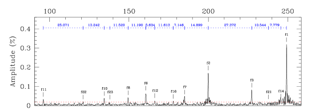
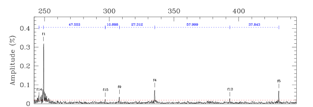
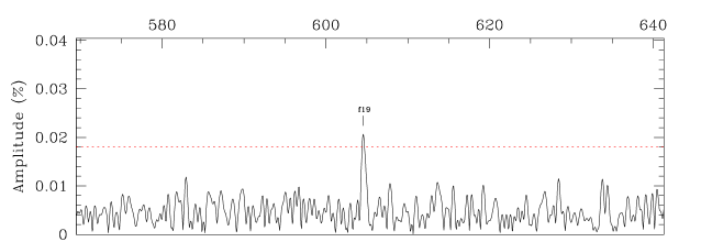
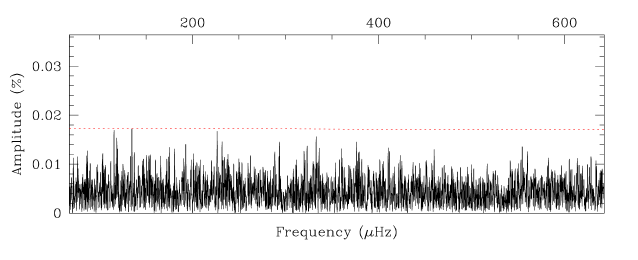
Figure 3: Three top panels show close-up views of the LSP of TIC 278659026 in the $g$-mode frequency range. The main frequencies listed in Table 1 are indicated, except the three peaks ($f_{18}$, $f_{17}$, and $f_{20}$; see text). In the top two panels, the separation in frequency between two consecutive peaks is indicated (the horizontal dotted-line segments). The horizontal dotted line in each panel indicates 4 times the median noise level used as an initial significance criterion. The bottom panel shows the residual after prewhitening all the frequencies.

It is important to note that, while most frequencies in the LSP could be prewhitened without leaving any residual behind, thus indicating strong stability over the 27.88 days of observation, significant remaining peaks could be found on two occasions. The first case occurred for $f_{7}$ at $185.014$ $\mu$Hz, which has $f_{18}$ at $184.479$ $\mu$Hz as a close-by companion, considering that the formal frequency resolution in Fourier space for these data is $0.415$ $\mu$Hz ($1/T$, where $T$ is the time baseline of the run). The other case is $f_{14}$ at $245.609$ $\mu$Hz which has $f_{20}$ at $245.102$ $\mu$Hz and $f_{17}$ at $246.027$ $\mu$Hz as close neighbors. From a pulsation perspective, these frequencies could very well be real independent modes of different degree $\ell$ that happen to have very close frequencies, barely resolved with the current data set. However, they may also be the signature of intrinsic amplitude and/or frequency modulations of the dominant peak, as discussed by Zong et al. (2016b, a, 2018). Therefore, as a precaution, we retain only the main (highest amplitude) peak of each complex, namely $f_{7}$ and $f_{14}$, for the detailed asteroseismic study of TIC 278659026.

Finally, we emphasize from Table 1 a few numbers characterizing the quality of these first TESS data obtained for a pulsating sdB star. With only one sector (27.88 days), targeting a bright ($V=11.57$), hot, and blue object (while TESS CCDs are red sensitive), the amplitude of the noise in Fourier space is around 0.0043% (43 ppm) in the $g$-mode frequency range, which is a remarkable achievement, especially considering the modest aperture of the instrument. We can expect this noise to be reduced further by up to a factor of $\sim 3.5$ for similar targets located in or near the CVZ, which could be observed for up to one year. We also note that the uncertainty on the measured frequencies is typically around one-tenth of the formal frequency resolution.

3 Asteroseismic analysis

3.1 Interpretation of the observed spectrum

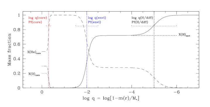
Figure 4: Illustration of the model parameters specifying the chemical stratification (see text for a full description of these parameters). The hydrogen, helium, carbon, and oxygen mass fractions are shown as a function of fractional mass depth, $\log q$, with plain, dashed, dot-dashed, and dotted curves, respectively.

Figure 3 shows a pulsation spectrum whose frequency distribution is very typical of $g$-mode pulsators observed from space (e.g., Charpinet et al., 2010; Østensen et al., 2010). The frequency spacings between consecutive peaks do not show quasi-symmetric structures that could clearly correspond to the signature of rotational splitting. Yet, we could argue that the projected rotational velocity ($v\sin i$) of $\sim 8$ km s^-1 proposed for TIC 278659026, if true (see Sect. 2.1), would correspond to a rotation period that is at most slightly less than one day ($P\sin i$) for a star of radius 0.15 $R_{\odot}$. Assuming a median statistical inclination of 60 , this period would be $\sim 0.82$ day, and the corresponding splittings $\sim 7$ $\mu$Hz for dipolar ($\ell=1$) $g$-modes and $\sim 11$ $\mu$Hz for quadrupolar ($\ell=2$) $g$-modes. Values close to these splittings can be seen between some of the observed peaks (see top panels of Fig. 3), but without the regularity that usually characterizes splittings at such slow rotation rates. Moreover, the typical average period spacings between consecutive $g$-modes of same degree in sdB stars generate frequency spacings in the range at which these pulsations are observed that are also of the same order without invoking rotation. To help distinguish between these two very different interpretations of the spectrum, it is important to recall that an unexplained discrepancy remains between the typical rotation rates inferred for sdB stars from spectroscopy (Geier et al., 2010; Geier & Heber, 2012) and the rotation periods measured from well-identified rotational splittings observed in pulsating sdB stars, in particular in those with very long time series delivered by the Kepler satellite (see, e.g., Kern et al., 2017 and other references provided by Charpinet et al., 2018). These splittings indicate in a very robust way that nearly all sdB pulsators, in particular the single pulsators, are extremely slow rotators with periods typically well above 10 days, at odds with the average $\sim 1$ day rotation timescale suggested by Geier & Heber (2012). Asteroseismology is clearly much more sensitive than line broadening analyses to very slow rotation rates. The question then arises whether the $\sim 8$ km s^-1 projected velocity found to be typical of sdB stars, which is not far above the limit of this method with the available spectra, is an actual measurement of the surface rotation of the star, an upper limit of it, or reflects an effect other than rotation causing additional broadening of the metal lines that has not been taken into account, such as line broadening by pulsation. This issue is well beyond the scope of the present paper, but clearly needs further investigation, possibly with the acquisition and analysis of very high-resolution spectra for a selection of pulsating and non-pulsating sdB stars.

For the present seismic study of TIC 278659026, we rely on previous observations of pulsating sdB stars, indicating extremely slow rotation rates. We interpret 20 observed frequencies (those marked with a “*” sign in Table 1) as independent sectoral ($m=0$) $g$-modes (first assumption) of degree $\ell=1$ or $\ell=2$ (second assumption). The first assumption follows from the above discussion and is further justified by the fact that the time baseline of the TESS run would probably be too short to resolve eventual $m\neq 0$ components in this framework. The observed frequencies can therefore be compared with the model frequencies computed assuming a nonrotating star, without any impact on the solution. The second assumption limits our search to dipole ($\ell=1$) and quadrupole ($\ell=2$) modes only, and is justified by the fact that cancellation effects over the stellar surface very strongly reduce the apparent amplitude of $\ell>2$ g-modes in sdB stars, except for very specific inclination angles of the pulsation axis relative to the line of sight. This has been clearly illustrated in Figure 11 of Charpinet et al. (2011), which shows that $\ell=3$ and 4 modes have apparent amplitudes already reduced by a factor of at least 10 owing to this effect. Such modes are therefore much less likely to be seen in the current data.

3.2 Method and models

The asteroseismic analysis of TIC 278659026 is based on the forward modeling approach developed over the years for hot subdwarf and white dwarf asteroseismology and described by, for example, Charpinet et al. (2005, 2008), Van Grootel et al. (2013), Charpinet et al. (2014c, 2015), and Giammichele et al. (2016). The method is a multidimensional optimization of a set of parameters, $\{p_{1},...,p_{n}\}$, defining the stellar structure of the star with the goal to minimize a “merit function” that measures the ability of that model to reproduce simultaneously all the observed pulsation frequencies. In the present analysis, the quality of the fit is quantified using a $\chi^{2}$-type merit function defined as

$$S^{2}(p_{1},...,p_{n})=\sum\limits_{i}^{N_{{\rm obs}}}\left(\frac{\nu_{{\rm obs,}i}-\nu_{{\rm th,}i}}{\nu_{{\rm obs,}i}}\right)^{2}\qquad,$$

where $N_{{\rm obs}}$ is the number of observed frequencies and $(\nu_{{\rm obs,}i},\nu_{{\rm th,}i})$ is a pair of associated observed and computed frequencies. We recall that this quantity, $S^{2}$, is minimized both as a function of the frequency associations, referred to as the first combinatorial minimization required because the observed modes are not identified a priori, and as a function of the model parameters, $\{p_{1},...,p_{n}\}$ (the second minimization). This optimization is carried out by the code lucy (see Charpinet et al., 2008), a Real-Coded Genetic Algorithm (RCGA) that can pursue multimodal optimization (i.e., searching simultaneously for multiple solutions) in any given multidimensional parameter space. This optimizer is coupled with a series of codes dedicated to the computation of the stellar structure itself (given a set of parameters), its pulsation properties, and to the matching of the computed frequencies with the observed frequencies.

Our current version of stellar models used for quantitative asteroseismology of sdB stars is an update of the Montr al third-generation (3G) models designed for an accurate computation of $g$-mode frequencies (Brassard & Fontaine, 2008, 2009; Van Grootel et al., 2010a; Charpinet et al., 2011). These models are complete hydrostatic stellar structures in thermal equilibrium computed from a set of parameters that define the main structural properties of the star. The implemented parameterization is inspired from full evolutionary calculations, which provide the guidelines to reproduce, for example, the general shape of the composition profiles in these stratified stars, but with additional flexibility. Such parameterized static structure models offer greater versatility, faster computations, and allow for much greater exploration of structural configurations in the spirit of constraining these from the pulsation modes themselves. The derived optimized structures are therefore seismic models that are mostly independent of the uncertainties still present in the physics that drives stellar evolution and shapes the chemical structure of the star over time, such as mixing and diffusion processes, mass losses, and nuclear reaction rates.

Table 2: Parameter space explored during optimization.

	First exploration	Second exploration
Parameter	Range covered	Range covered
$M_{*}/M_{\odot}$	$[0.30,0.60]$	$[0.30,0.45]$
$\log q({\rm env})$	$[-4.0,-1.5]$	$[-3.0,-1.5]$
$\log q({\rm H/diff})$	$[-5.0,-2.0]$	$[-5.0,-2.0]$
$X({\rm H})_{\rm envl}$	$[0.70,0.75]$	$[0.70,0.75]$
Pf(envl)	$[1,10]$	$[1,10]$
Pf(H/diff)	$[1,10]$	$[1,10]$
$\log q({\rm core})$	$[-0.5,-0.1]$	$[-0.4,-0.15]$
Pf(core)	$[1,150]$	$[50,150]$
$X({\rm He})_{\rm core}$	$[0.0,1.0]$	$[0.0,1.0]$
$X({\rm O})_{\rm core}$	$[0.0,1.0]$	$[0.0,1.0]$

Compared to the former 3G models used by, for example, Van Grootel et al. (2010a, b), Charpinet et al. (2011), and Van Grootel et al. (2013), the most important improvement is that our current stellar structures for sdB stars now implement a more realistic hydrogen-rich envelope with double-layered hydrogen and helium composition profiles. This addition was motivated by the fact that diffusion of helium through gravitational settling does not have time, during the typical duration of the core helium burning phase, to completely sink below the envelope when this envelope is relatively thick (see, e.g., Hu et al., 2009, 2010). This is most likely to be relevant for $g$-mode sdB pulsators that are found among the cooler sdB stars with thicker envelopes, while the hotter $p$-mode sdB pulsators all have thinner envelopes that quickly become fully hydrogen-pure. Consequently, in the present analysis, the assumption of a pure hydrogen envelope used so far is better replaced by an envelope that may still contain some helium, with a transition from pure hydrogen (at the top) to a mixture of H+He (at its base). The technical implementation of this double-layered H+He composition profile is identical in its principle to the implementation of a double-layered helium envelope in DB white dwarf models, as described recently in the Methods section of Giammichele et al. (2018).

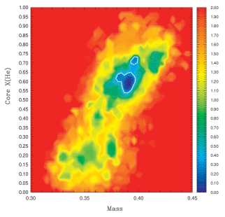
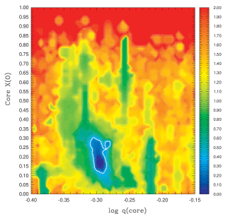
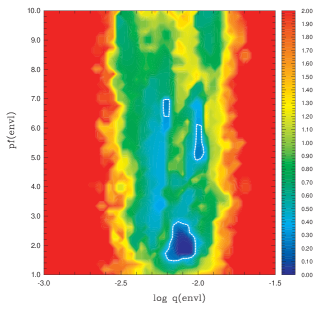
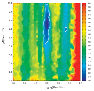
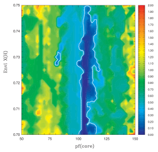
Figure 5: $\log S^{2}$ projection maps for pairs of primary model parameters showing location and shape of best-fitting regions in parameter space (see text for more details). The value $S^{2}$ is normalized to one at minimum and the color scale is logarithmic. Dark blue indicates the best-fit regions and the dotted contour line is an estimate of the $1\sigma$ confidence level, obtained in a similar way to that described by Brassard et al. (2001).

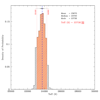
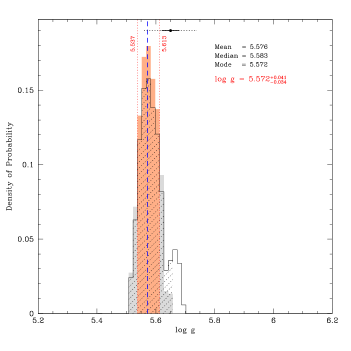
Figure 6: Probability distributions for $T_{{\rm eff}}$ (top panel) and $\log g$ (bottom panel) around the optimal seismic solution for TIC 278659026. Two distributions are superimposed: one resulting from the full sample including all secondary optima (black histograms) and the other computed from a restricted sample focusing on the global optimum (red and gray shaded histogram). This restricted sample is built from excluding parts of the parameter space as indicated in the bottom panel for example and in some panels of Fig. 7, 8, 9, and 10, by bins that do not show the dotted hatched areas. The red-shaded areas delimited by the red vertical dotted lines contain 68% of the restricted probability distribution and provide our estimate of the $1\sigma$ error range for the quantity considered. For internal physical consistency of the derived parameters, the adopted value is that from the optimal model (blue vertical dashed line), which closely corresponds to the mode (maximum) of the distribution. The black dots, and their associated horizontal lines, indicate the measurement obtained independently from spectroscopy, and the $1\sigma$ (solid) and $3\sigma$ (dotted) ranges around that value.

The input parameters needed to fully define the stellar structure with these improved models are the following. First the total mass, $M_{*}$, of the star has to be given. All additional parameters specify the chemical stratification inside the star, as illustrated in Fig. 4. We start with five parameters defining the double-layered He and H envelope structure. The first parameter is the fractional mass of the outer hydrogen-rich envelope, $\log q({\rm env})=\log(M_{{\rm env}}/M_{*})$, corresponding in effect to the location of the deepest transition of the double-layered structure, from the pure He mantle to the mixed He+H region at the bottom of the envelope. The second parameter is the fractional mass of the pure hydrogen layer at the top of the envelope, $\log q({\rm H/diff})=\log(M_{{\rm H/diff}}/M_{*})$, which fixes the location of the transition between the He+H mixed layer to the pure hydrogen region. The shape (or extent) of both transitions are controlled by two additional parameters, $Pf({\rm envl})$ and $Pf({\rm H/diff})$ (see the Methods section of Giammichele et al., 2018 for details). The remaining parameter, $X({\rm H})_{{\rm envl}}$, closes the specification of the envelope structure by fixing the mass fraction of hydrogen in the mixed He+H region of the envelope. We also note for completeness that the stellar envelope incorporates a nonuniform iron distribution computed assuming equilibrium between radiative levitation and gravitational settling (see Charpinet et al., 1997, 2001). In addition to this set of parameters, the core structure has to be defined by specifying the fractional mass of the convectively mixed core, $\log q({\rm core})=\log(1-M_{{\rm core}}/M_{*})$, which sets the position of the transition between the CO-enriched core (owing to helium burning) with the surrounding helium mantle. How steep (or wide) is this transition is specified by the profile factor, $Pf({\rm core})$, and the composition of the core is determined by the two parameters $X({\rm He})_{{\rm core}}$ and $X({\rm O})_{{\rm core}}$ providing the mass fraction of helium and oxygen (the complement being carbon, with $X({\rm C})_{{\rm core}}=1-X({\rm He})_{{\rm core}}-X({\rm O})_{{\rm core}}$). A full EHB stellar structure is therefore entirely specified with the ten primary parameters mentioned above. Other secondary quantities, such as the effective temperature, surface gravity, or stellar radius, simply derive from the converged stellar model in hydrostatic and thermal equilibrium.

Finally, we recall that the seismic properties of a given stellar model are computed using the Montr al pulsation code (Brassard et al., 1992; Brassard & Charpinet, 2008). Calculations in the adiabatic approximation are sufficient for the present purposes and much more efficient numerically than the full nonadiabatic treatment.

3.3 Search for an optimal seismic model

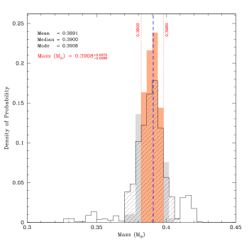
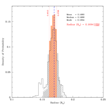
Figure 7: Same as Figure 6 but for the mass (top panel) and radius (bottom panel) of TIC 278659026.

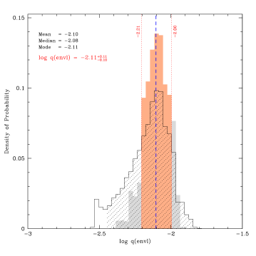
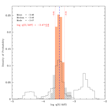
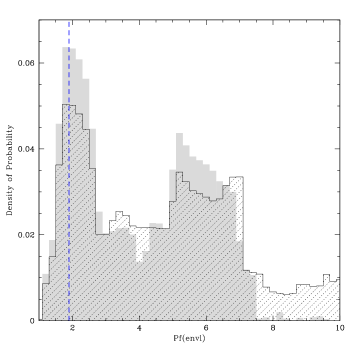
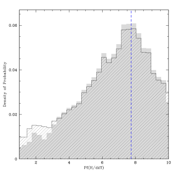
Figure 8: Same as Figure 6 but for the remaining envelope structural parameters defining the seismic model of TIC 278659026. No errors are estimated for Pf(envl) and Pf(H/diff) considering the spread of their distribution.

The search for an optimal solution that reproduces the seismic properties of TIC 278659026 was conducted in the multidimensional space defined by the ten primary model parameters discussed in the previous subsection. A first exploratory optimization with the code lucy was performed to cover the largest possible domain in parameter space, relevant for virtually all configurations that could potentially correspond to a typical sdB star. This wide domain is defined in the second column of Table 2 and the search was done without considering the constraint available from spectroscopy at this stage. Remarkably, this first calculation pointed toward a basin of solutions located very close to the spectroscopic values of $\log g$ and $T_{{\rm eff}}$, suggesting a sdB star of relatively low mass. This helped to reduce the size of the search space for the ultimate convergence toward the best-fit solution.

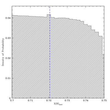
Figure 9: Same as Figure 8 but for the mass fraction of hydrogen, $X({\rm H})_{{\rm envl}}$, at the bottom of the hydrogen-rich envelope.

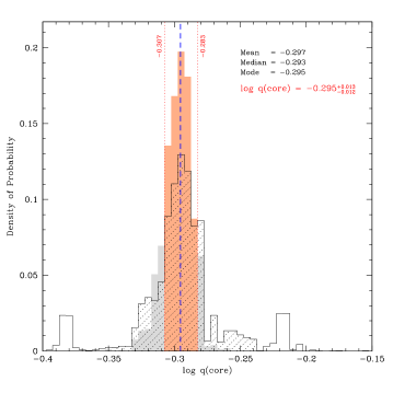
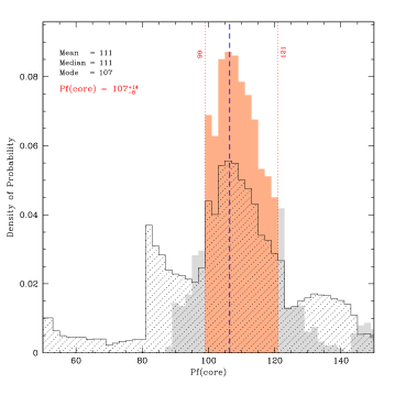
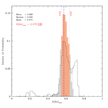
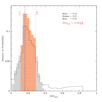
Figure 10: Same as Figure 6 but for the core structural parmameters defining the seismic model of TIC 278659026.

The second and ultimate round of optimization was conducted within the ranges given in the third column of Table 2. This time the spectroscopic values of $\log g$ and $T_{{\rm eff}}$ were introduced in the optimization process as additional external constraints degrading progressively the merit function when a computed model has $\log g$ and/or $T_{{\rm eff}}$ that differ from spectroscopy by more than a tolerance range set to be $3\sigma$ (three times the spectroscopic error). The optimizer lucy was configured to aggressively converge each potential model solution found in parameter space by combining the GA search with a simplex optimization round. This step ensures that the global and eventual local minima of the merit function are effectively reached. This second round of calculation required the computation and comparison with observed frequencies of 1,555,425 seismic models. We point out that the parameter $X({\rm H})_{{\rm envl}}$ was kept within the narrow $0.70-0.75$ range from the assumption that the progenitor of TIC 278659026 had a homogeneous H+He envelope close to solar composition when it entered the EHB phase. Yet, the possibility that the star may have a significantly different H/He ratio in the envelope as a consequence of passed episodes of mixing related to binary evolution is not totally excluded. The impact of widening this range is discussed in Sect. 3.3.3 and Appendix A.

Table 3: Derived properties of TIC 278659026.

Quantity	Value derived	Other
	from seismology	Measurement
Primary quantitiesa
$M_{*}/M_{\odot}$	$0.391\pm 0.009$	$0.390\pm 0.091^{{\ddagger}}$
$\log q({\rm env})$	$-2.11\pm 0.11$	…
$\log q({\rm H/diff})$	$-3.47\pm 0.16$	…
$X({\rm H})_{\rm envl}$	$\sim 0.72$	…
Pf(envl)	$\sim 1.87$	…
Pf(H/diff)	$\sim 7.7$	…
$\log q({\rm core})$	$-0.295\pm 0.013$	…
Pf(core)	$107\pm 14$	…
$X({\rm He})_{\rm core}$	$0.575_{-0.027}^{+0.063}$	…
$X({\rm O})_{\rm core}$	$0.16_{-0.05}^{+0.13}$	…
Secondary quantitiesb
$T_{\rm eff}$ (K)	$23740\pm 640$	$23720\pm 260^{c}$
$\log g$	$5.572\pm 0.041$	$5.650\pm 0.030^{c}$
$R/R_{\odot}$	$0.1694\pm 0.0081$	…
$M_{\rm H}/M_{\odot}$	$0.0037\pm 0.0010^{{\dagger}}$	…
$M_{\rm core}/M_{\odot}$	$0.198\pm 0.010$	…
$X({\rm C})_{\rm core}$	$0.27_{-0.14}^{+0.06}$	…
$L/L_{\odot}$ ($T_{\rm eff}$, $R$)	$8.2\pm 1.7$	$8.2\pm 1.1^{c}$
$M_{V}$ ($g$, $T_{\rm eff}$, $M_{*}$)	$4.92\pm 0.15^{d}$	…
$M_{B_{p}}$ ($g$, $T_{\rm eff}$, $M_{*}$)	$4.70\pm 0.16^{d}$	…
($B$-$V$)0	$-0.225\pm 0.007^{d}$	…
($B_{p}$-$R_{p}$)0	$-0.404\pm 0.011^{d}$	…
$V$	…	$11.57\pm 0.09^{e}$
($B$-$V$)	…	$-0.22\pm 0.10^{e}$
$B_{p}$	…	$11.433\pm 0.008^{f}$
($B_{p}$-$R_{p}$)	…	$-0.398\pm 0.009^{f}$
$E$($B$-$V$)	$0.005\pm 0.107$	…
$E$($B_{p}$-$R_{p}$)	$0.005\pm 0.020$	…
$d_{\rm parallax}$ (pc)	…	$203.7\pm 2.1^{g}$
$d_{V}$ (pc)	$212.2\pm 57.0^{h}$	…
$d_{B_{p}}$ (pc)	$220.9\pm 20.4^{i}$	…

^aOptimized model parameters (see text)
^‡From fitting the SED and using Gaia DR2 parallax (see text)
^bQuantities derived from the computed models
^cFrom spectroscopy (Németh et al. 2012)
^†$\log\frac{M(\rm H)}{M_{*}}=\log q({\rm envl})+C=-2.0251$; $C$ comes from the model
^dFrom a model atmosphere with $\log(\frac{{\rm He}}{{\rm H}})=-3.0$
^eFrom Høg et al. 2000
^fFrom Gaia DR2 photometry
^gFrom Gaia DR2 parallax, $\varpi=4.910\pm 0.051$ mas
^h$d=213.8\pm 23.4$ without correction for extinction
ⁱ$d=221.9\pm 16.6$ without correction for extinction

The first result emerging from the optimization in the 10D parameter space is the identification of a solution for TIC 278659026 that clearly dominates over other secondary options. This is illustrated in Fig. 5, showing the 2D projection maps of $\log S^{2}$ ($S^{2}$ being normalized to one at minimum in this context) for various pairs of the ten model parameters. The approximate reconstruction of the topology of $S^{2}$ derives from the sampling of the merit function by the optimizer during the search. While $\log S^{2}$ has a rather complex structure with several local dips, as expected, a dominant global minimum is found. Moreover, all parameters appear well constrained (i.e., precisely localized around the optimum), except for the hydrogen content in the mixed He+H region at the base of the envelope, $X({\rm H})_{{\rm envl}}$, whose minimum is an elongated valley (see also Appendix A), and, to a lesser extent, the shape factors $Pf({\rm envl})$ and $Pf({\rm H/diff})$ that also tend to spread more over their explored range than other parameters.

The identification of a well-defined global minimum dominating all the other optima allows for the selection of an optimal seismic model of TIC 278659026 and the determination of its parameters through the series of plots provided in Figs. 6, 7, 8, 9, and 10. These histograms show the probability distributions for the most relevant parameters through marginalization. As described in, for example, Van Grootel et al. (2013), these distributions are evaluated from the likelihood function ($\propto e^{-\frac{1}{2}S^{2}})$ and are useful to estimate the internal error associated with each parameter value. In this work, slightly differing from previous similar studies, the adopted parameter values are those given by the optimal model solution, which closely corresponds to the mode (maximum) of their associated distribution. This ensures internal physical consistency between all values, since they exactly represent the optimal seismic model. Moreover, since some histograms can differ significantly from the normal distribution, for instance when secondary peaks are visible, we chose to estimate these errors by constructing a second distribution computed from a restricted sample in the vicinity of the dominant solution, thus filtering out secondary optima (see the caption of Fig. 6 for more details). All the values derived from the optimal seismic model and their estimated errors are provided in Table 3, along with other independent measurements of the same quantity when available, for comparison purposes.

3.3.1 Global parameters

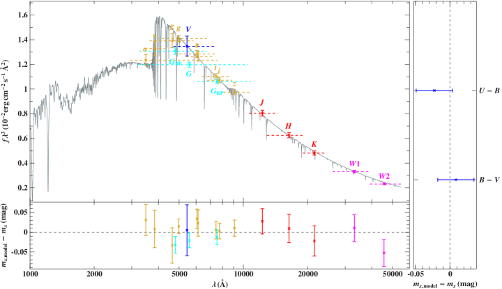
Figure 11: Comparison of synthetic and observed photometry: The top panel shows the SED. Colored data points represent the filter-averaged fluxes, which were converted from observed magnitudes; the respective filter width is indicated by dashed horizontal lines. The gray solid line represents a synthetic spectrum computed from a model atmosphere with the best-fit effective temperature. The panels at the bottom and on the right-hand side show the differences between synthetic and observed magnitudes and colors. The following color codes are used to identify the photometric systems: Johnson (blue), APASS $g$, $r$, $i$ (yellow), SkyMapper (yellow), Gaia (cyan), 2MASS (red), and WISE (magenta).

The seismic model uncovered for TIC 278659026 has $T_{{\rm eff}}$ and $\log g$ values in very close agreement – both within or very close to the $1\sigma$ error bars – with the values measured independently from spectroscopy (Fig. 6). This demonstrates a remarkable consistency of the solution that was not guaranteed a priori. We also find that TIC 278659026 has a tightly constrained radius of $0.1694\pm 0.0081$ $R_{\odot}$ and a mass of $0.391\pm 0.009$ $M_{\odot}$ (Fig. 7). The latter is significantly less than the canonical mass of $\sim 0.47$ $M_{\odot}$ expected for typical sdB stars, which indeed explains why TIC 278659026 has a rather high surface gravity (and small radius) given its relatively low effective temperature, which places it somewhat below the bulk of hot subdwarfs in a $\log g-T_{{\rm eff}}$ diagram. It is the first $g$-mode pulsating sdB star (and only second pulsator, if we include the V361 Hya stars) with such a low mass determined precisely from asteroseismology. Therefore, this object bears a particular interest in the context of determining the empirical mass distribution of field sdB stars (see, Fontaine et al., 2012).

A second important test of the reliability of the seismic solution is provided by the comparison, in Table 3, between the distance of the star measured from the available Gaia DR2 trigonometric parallax and the “seismic distance” evaluated from the optimal model properties. The latter is obtained by computing a representative model atmosphere of TIC 278659026 based on $T_{{\rm eff}}$ and $\log g$ derived from the seismic model (see, Fontaine et al., 2019). The synthetic spectrum computed from this model atmosphere is then used to derive absolute magnitudes and theoretical color indices in the photometric band-passes of interest. Combined with photometric measurements, these values give access to estimates of the interstellar reddening and ultimately to the distance modulus (corrected by the extinction, which is found to be almost negligible in the present case). We find that the seismic distance obtained for TIC 278659026 is in very close agreement – compatible with $1\sigma$ errors – with the distance measured by Gaia. This indicates that the global properties of the star obtained from our seismic analysis, in particular its effective temperature, mass, and radius, are indeed accurate to the quoted precision.

Table 4: List of the observed magnitudes used to fit the SED (see Fig. 11).

System	Bandpass	Magnitude
Gaia	G	$11.5928\pm 0.0009$
Gaia	GRP	$11.8308\pm 0.0018$
Gaia	GBP	$11.4327\pm 0.0083$
WISE	W1	$12.413\pm 0.023$
WISE	W2	$12.512\pm 0.023$
2MASS	J	$12.152\pm 0.021$
2MASS	H	$12.264\pm 0.025$
2MASS	K	$12.375\pm 0.027$
SDSS	$g$	$11.387\pm 0.033$
SDSS	$r$	$11.792\pm 0.022$
SDSS	$i$	$12.144\pm 0.010$
Johnson	B-V	$-0.23$
Johnson	U-B	$-0.89$
Johnson	V	$11.62$
SkyMapper	$u$	$11.283\pm 0.028$
SkyMapper	$v$	$11.309\pm 0.035$
SkyMapper	$g$	$11.444\pm 0.002$
SkyMapper	$r$	$11.767\pm 0.013$
SkyMapper	$i$	$12.208\pm 0.006$
SkyMapper	$z$	$12.521\pm 0.007$

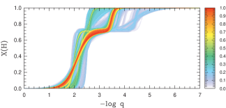
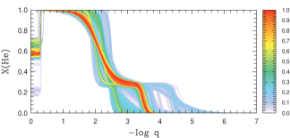
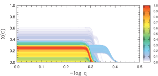
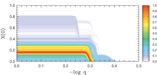
Figure 12: Probability distributions (color scale) normalized to one at maximum as functions of the fractional mass depth, $\log q=\log[1-m(r)/M_{\star}]$, obtained, from top to bottom, for the mass fraction of hydrogen, helium, carbon, and oxygen inside TIC 278659026. The red areas indicate the values, as functions of $\log q$, corresponding to the best-matching seismic models. These distributions are derived from the evaluation of 1,555,425 stellar models calculated during exploration of parameter space.

As a last complementary check, we derive interstellar extinction from the spectral energy distribution (SED) and colors by comparing all available photometric measurements for TIC 278659026 to synthetic measurements calculated from an appropriate model atmosphere (see Fig. 11). The photometry used in Fig. 11 (see Table 4) covers from the $u$-band to the infrared $J$, $H$, $K$ (2MASS; Skrutskie et al., 2006) and $W1$, $W2$ (WISE; Cutri & et al., 2013). The Johnson $V$ magnitude and colors for this specific test were taken from O’Donoghue et al. (2013). The SkyMapper (Wolf et al., 2018), APASS $g$, $r$, $i$ (Henden et al., 2016), and Gaia (Gaia Collaboration et al., 2018) magnitudes were also included. Details of the model spectra and the fitting procedure are given by Heber et al. (2018). The angular diameter obtained from this fit is $\theta=\left(3.42_{-0.06}^{+0.05}\right)\times 10^{-11}$ rad, and interstellar reddening is found to be zero (i.e., $E$(B-V) $\leq 0.009$; consistent with the value given in Table 3). This approach also estimates a photometric effective temperature that is well within $1\sigma$ agreement with other methods, giving $T_{{\rm eff}}=23600_{-400}^{+700}$ K. Using the high-precision parallax provided by Gaia DR2, $\varpi=4.910\pm 0.051$, combined with the angular diameter and the surface gravity, the stellar mass can be obtained through the relation $M=g\,\Theta^{2}/(4G\,\varpi^{2}$). This results in a mass of $M=0.390\pm 0.091$ $M_{\odot}$, based on the atmospheric parameters from Németh et al. (2012) using a conservative estimate of 0.1 dex for the error on $\log g$, instead of the statistical uncertainties quoted by the authors. This value is remarkably consistent with the mass derived from the asteroseismic solution. We close this discussion by noting that, interestingly, the WISE W2 measurement rules out the presence of a companion earlier than type M5 or M6 (assuming a $3\sigma$ excess at W2 above the expected flux coming from the sdB photosphere).

3.3.2 Potential implications in terms of evolution

According to Han et al. (2002, 2003), such a low-mass sdB star is most probably produced by the first stable Roche lobe overflow (RLOF) channel, although there is presently no indication of the presence of a stellar companion. The low mass inferred suggests that TIC 278659026 must have started helium burning in nondegenerate conditions, i.e., before reaching the critical mass that triggers the helium flash. Stellar evolution calculations show that main sequence stars with masses above $\sim 2$ $M_{\odot}$ ignite helium before electron degeneracy occurs, and consequently have less massive cores. TIC 278659026 could, in this context, become the first evidence of a rare sdB star that originates from a massive ($\gtrsim 2$ $M_{\odot}$) red giant, an alternative formation channel investigated by Hu et al. (2008). Finally, we note that the inferred mass and the presence of pulsations at such high effective temperature rule out the suggestion from Kawka et al. (2015) that TIC 278659026 may be an ELM white dwarf progenitor.

3.3.3 Internal structure

Beyond the determination of the fundamental parameters characterizing TIC 278659026, our asteroseismic analysis provides insight into the internal structure of the star, in particular its chemical composition and stratification. Interesting constraints on the double-layered envelope structure are indeed obtained (Fig. 8, 9 and Table 3), along with measurements of the helium-burning core properties (Fig. 10 and Table 3). The various parameters defining these structures fully determine the chemical composition distribution inside the best-fit model for the four main constituents, H, He, C, and O, and Fig. 12 provides a more convenient way to visualize these profiles and their uncertainties. This plot is constructed from the composition profiles in the 1,555,425 models evaluated by the optimizer during its exploration of the parameter space (see Giammichele et al., 2017 who introduced similar plots in a white dwarf context). Each model (and therefore each composition profile) has a $S^{2}$ value attributed regarding its ability to match the pulsation frequencies of TIC 278659026. Consequently, probability distributions for the amount of H, He, O, and C (the complement of He and O in the core) as functions of the fractional mass depth, $\log q=\log(1-m(r)/M_{*})$, can be evaluated. We find from these distributions that a well-defined region corresponding to best-fitting models emerge for each element, thus materializing the chemical stratification of TIC 278659026 as estimated from asteroseismology. Significantly weaker secondary solutions can also be seen in these diagrams.

From the seismic solution obtained, we find that TIC 278659026 has a thick envelope by sdB standards, with $\log q({\rm envl})=-2.11\pm 0.11$, where a double-layered structure for the He+H profile indicates that gravitational settling has not yet completely segregated helium from hydrogen. Such a configuration is indeed expected for a cool sdB star such as TIC 278659026, since envelope masses of EHB stars are strongly correlated with effective temperature and element diffusion does not have time in principle to affect the base of a thick envelope. The mass fraction of hydrogen present in this mixed He+H region is not really constrained, owing to a very weak sensitivy of the $g$-mode pulsation frequencies to this parameter, although the optimal seismic model gives $X({\rm H})_{{\rm envl}}\sim 0.72$. We note that we imposed this quantity to be close to the proportion expected in the solar mixture (by exploring only a narrow range of values), assuming that the sdB envelope is the remnant of the original main sequence stellar envelope with unchanged composition. However, in light of Fig. 9, we might argue that a global optimum may lie outside of the range considered. Moreover, the evolution history of the progenitor of TIC 278659026 may not necessarily lead to a nearly solar H/He ratio in the envelope. We have therefore, as a check, extended the analysis to a wider range of $X({\rm H})_{{\rm envl}}$ values with additional calculations described in Appendix A. The latter shows that 1) there is no preferred value for $X({\rm H})_{{\rm envl}}$ in the $\sim 0.58-0.86$ range that would lead to a significantly better fit; 2) models with He-enriched envelopes above $Y\gtrsim 0.42$ seem excluded; and 3) our identified optimal solution remains entirely valid, although some derived parameters may have slightly larger error estimates propagated from the wider range considered for the envelope hydrogen content. After this test, we therefore confidently keep the solution identified from our more constrained calculations as the reference.

The inner core structure is also unveiled, pointing to a rather large mixed core with a fractional mass $\log q({\rm core})=-0.295\pm 0.013$, corresponding to $M_{{\rm core}}=0.198\pm 0.010$ $M_{\odot}$. This size is reached while the estimated remaining helium mass fraction in that region is $X({\rm He})_{{\rm core}}=0.575{}_{-0.027}^{+0.063}$. TIC 278659026 is therefore close to the mid-stage of its helium-burning phase, as it has transformed about 43% of its helium into carbon and oxygen. We point out that the value obtained for the core size is comparable to some estimates already provided for this quantity by Charpinet et al. (2011) for the star KIC 02697388 (solution 2) and by Van Grootel et al. (2010b) for the star KPD 0629-0016. The latter in particular, although more massive as it has a canonical mass of $0.471\pm 0.002$ $M_{\odot}$, happens to be nearly at the same stage of its core helium-burning phase, with $\sim 59\%$ (in mass) of helium left in the central region, while its estimated core size is $\log q({\rm core})=-0.27\pm 0.01$ ($M_{{\rm core}}=0.22\pm 0.01$ $M_{\odot}$). Nonetheless, Van Grootel et al. (2010a) also provided a seismic estimate of the core mass for the sdB pulsator KPD 1943+4058, but obtained a significantly larger measurement for this quantity. This star may need to be reinvestigated with our most recent modeling tools applied to the full data set now available; the Van Grootel et al., 2010a analysis was based on Kepler’s Q0 light curve only. Remarkably, and for the first time in a sdB star, our present seismic modeling of TIC 278659026 also provides an estimate for the oxygen mass fraction in the helium burning core. We find that $X({\rm O})_{{\rm core}}=0.16{}_{-0.05}^{+0.13}$ and consequently the estimated carbon mass fraction is $X({\rm C})_{{\rm core}}=0.27{}_{-0.14}^{+0.06}$. These values, along with knowing the size of the core, are of high interest as they are directly connected with the uncertain rate of the ${}^{12}{\rm C}(\alpha,\gamma)^{16}{\rm O}$ nuclear reaction, which is fundamental in many areas of astrophysics.

3.3.4 Frequency match and mode identification

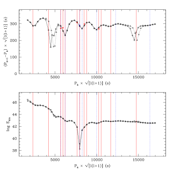
Figure 13: Top panel: Period spectrum corresponding to the optimal seismic model obtained for TIC 278659026 and represented in terms of the reduced period spacing, $(P_{k+1}-P_{k}).\sqrt{\ell(\ell+1)}$ (in seconds) as a function of reduced period, $P_{k}.\sqrt{\ell(\ell+1)}$ (in seconds). Open squares connected by plain segments show the $\ell=1$ series of modes and open triangles connected by dotted segments are $\ell=2$ modes. The range of radial orders covered spans $k=5$ to $k=60$, as in Table 5. Plain and dotted vertical lines indicate the reduced periods of the observed modes matched to $\ell=1$ and $\ell=2$ modes, respectively. When two observed modes of same degree have consecutive radial orders, an observed reduced period spacing is also indicated (filled squares and filled triangles for $\ell=1$ and $\ell=2$ modes, respectively). Bottom panel: Same as above, but for the logarithm of the kinetic energy (or inertia), $\log E_{{\rm kin}}$, of the modes as a function of reduced period.

The optimal seismic model uncovered for TIC 278659026 provides the closest match to the observed frequencies obtained thus far for a g-mode pulsating sdB star. With an average relative dispersion $|\overline{\Delta X/X}|=0.07\%$ ($X=P$ or $\nu$), which corresponds on an absolute scale to $|\overline{\Delta P}|=3.16$ second and $|\overline{\Delta\nu}|=0.161$ $\mu$Hz for 20 frequencies matched simultaneously, this fit outperforms previous comparable studies presented by Van Grootel et al. (2010a, b) and Charpinet et al. (2011) by a factor $\sim 3-5$ on the achieved relative dispersion. This significant gain in matching precision is clearly due to the improvements implemented in stellar models used in the present analysis relative to these older studies, that is the inclusion of a double-layered hydrogen-rich envelope (see Section 3.1). We point out that this ability to better reproduce the observed oscillation spectrum is certainly the main factor that has allowed us to extract more information about the internal structure of TIC 278659026. We also find that our best fit reaches an absolute precision in frequency that is $\sim 2.5$ times better than the formal resolution of this TESS observing run ($1/T=0.415$ $\mu$Hz). However, since the actual uncertainty on each frequency measurement is on the order of one-tenth of the formal resolution (Table 1), the match is not perfect and significant room still remains to improve our seismic modeling further. A better description of the helium-burning core boundary to produce profiles that comply more accurately to those produced by, for example, semi-convection is among future improvements that we plan to introduce.

All the details of the $g$-mode spectrum of the optimal model, frequency fit, and associated mode identification are given in Table 5 and illustrated in Fig. 13. The table provides, for each mode, the degree $\ell$ and radial order $k$, the computed adiabatic frequency and period ($\nu_{{\rm th}}$ and $P_{{\rm th}}$), their corresponding matched frequency and period ($\nu_{{\rm obs}}$ and $P_{{\rm obs}}$) when available, the logarithm of the kinetic energy (or inertia) of the mode ($\log E_{{\rm kin}}$; see, e.g., Charpinet et al., 2000), the first-order Ledoux coefficient for slow rigid rotation ($C_{k\ell}$), and the relative and absolute differences between the observed and computed values $\Delta X/X$, $\Delta P$, and $\Delta\nu$, when available. We find that the 20 independent frequencies of TIC 278659026 are well interpreted as 13 $\ell=1$ and 7 $\ell=2$ $g$-modes of low-to-intermediate radial orders ranging from $k=7-57$. The observed spectrum is clearly incomplete, with many undetected eigenfrequencies that are present in the model. Many of these unseen frequencies may be excited by the driving engine, but to amplitude levels that are simply below the detection threshold reached. They may also not be exited at all, but linear nonadiabatic calculations indicate that all modes within the instability range should in principle be driven (Fontaine et al., 2003; Jeffery & Saio, 2007; Bloemen et al., 2014). The mechanisms controlling mode amplitude saturation are not well known. Moreover, amplitudes can change over long timescales in $g$-mode sdB pulsators, probably because of nonlinear mode interactions, as documented by Zong et al. (2016a, 2018). In this context, bottom panel of Fig. 13 suggests that modes of lowest inertia (or kinetic energy), which are susceptible to be excited to higher intrinsic amplitudes for a given amount of energy, seem indeed to be those most seen in the spectrum of TIC 278659026. Hence, the overall amplitude distribution (and detectability) of $g$-modes in sdB pulsators probably has mode inertia as one of its controlling factors, but other effects play an important role too.

Despite the relatively sparse distribution, several observed frequencies are grouped into two or three modes of consecutive radial order. The top panel of Fig. 13 illustrates the pulsation spectrum of the best-fit model and the matched observed modes in terms of their reduced period spacing, $\Delta P_{k}=(P_{k+1}-P_{k}).\sqrt{\ell(\ell+1)}$, plotted as a function of reduced period, $P_{k}.\sqrt{\ell(\ell+1)}$, for the dipole and quadrupole series. This representation highlights a series of oscillations and dips that occur around the theoretical average reduced period spacing, $\Pi_{0}$, whose value is 278.4 s for the optimal model; these are typical of trapping effects generated by rapid changes of the chemical composition, for example, at the core edge or at the mantle-envelope transition (see Charpinet et al., 2000, 2002a, 2002b, 2014a, and references therein). We note that the period spacings derived from $\Pi_{0}$ are comparable to those observed for the $g$-dominated mixed modes in core helium-burning red giants (O’Toole, 2012), thus underlining that the convectively mixed He-burning cores of EHB and red clump stars should be similar. Moreover, we point out that trapping affecting the mixed modes also occurs in red giant stars (Bedding et al., 2011). As expected from asymptotic relations, all modes of the same radial order but different degree $\ell$ almost always overlap in the reduced period space and follow the same patterns. We note a slight distortion to this rule around two dips in which the trapping occurs with a shift of $\Delta k=1$ for $\ell=2$ modes compared to their $\ell=1$ counterpart. This distortion appears related to the sharp transition at the core boundary, which has the peculiarity to be located close to the inner turning point of the gravity waves in their resonant cavity. Overall, we find that the observed periods and their identification match the model spectrum properties well. However, small discrepancies are still noticeable, reflecting, as mentioned previously, the greatly improved but still imperfect models used in this asteroseismic analysis.

4 Summary and conclusions

We have reported on the discovery of a new bright $g$-mode pulsating sdB star, TIC 278659026 (EC 21494-7078), by the NASA/TESS mission. This object is just one of the hundreds of evolved compact stars (mostly hot subdwarfs and white dwarfs) monitored with the 120 s cadence mode in the first TESS sector. This effort is part of a larger program driven by TASC Working Group 8 to survey thousands of bright evolved compact stars for variability. The data consists of 27.88 days of photometry with a nearly continuous coverage, thus offering a clear view of the pulsation spectrum of TIC 278659026. The analysis of the time series revealed the presence of many frequencies in the 90–650 $\mu$Hz range, among which 20 are interpreted as independent low-degree ($\ell=1$ and 2) gravity modes later used to provide strong seismic constraints on the structure and fundamental parameters of the star.

The asteroseismic investigation of TIC 278659026 was conducted with our current modeling and optimization tools. These implement a forward modeling approach developed over the past 15 years and described in some detail in papers by Van Grootel et al. (2013), Giammichele et al. (2016), and references therein. Compared to former analyses of $g$-mode sdB pulsators, we used an improved version of the Montr al 3G stellar models (Van Grootel et al., 2010a, b; Charpinet et al., 2011) implementing a more complex envelope structure that allows for double-layered hydrogen and helium profiles. Such profiles are characteristic of the outcome of gravitational settling for the coolest hot subdwarfs, when helium lacks time to completely sink below their relatively thick envelopes during the lifetime of the star on the EHB. Former 3G models assumed pure hydrogen envelopes that were not fully appropriate to analyze the coolest $g$-mode sdB pulsators.

The extensive search for a best-fit seismic model reproducing the 20 frequencies that characterize TIC 278659026 led to the identification of a well-defined solution in close agreement with available constraints on $T_{{\rm eff}}$ and $\log g$ derived from spectroscopy (Németh et al., 2012). The solution also agrees remarkably well with the distance measured independently from the Gaia trigonometric parallax, through a comparison with the seismic distance estimated from the model properties (see Section 3.3.1 and Table 3), and with the mass estimated from combining the fit of the SED and the Gaia parallax. All constitute important tests validating the accuracy of the identified seismic model. Through this solution, asteroseismology is giving us extensive information on fundamental parameters and internal structure in TIC 278659026. In particular, we find that this star has a mass of $0.391\pm 0.009$ $M_{\odot}$, which is significantly lower than the canonical mass of $0.47$ $M_{\odot}$ characterizing most sdBs, and could originate from a massive ($\gtrsim 2$ $M_{\odot}$) red giant progenitor.

Other notable results include constraints on the chemical stratification inside the star. We found, in particular, that TIC 278659026 has a rather thick H-rich envelope, with $M(H)=0.0037\pm 0.0010$ $M_{\odot}$ (computed from $\log q({\rm envl})=-2.11\pm 0.11$; see Table 3), whose structure includes a double-layered He and H distribution caused by still ongoing gravitational settling of helium. The core, for its part, is found to be more extended than typically predicted by standard evolution models, reaching a mass of $0.198\pm 0.010$ $M_{\odot}$ ($\log q({\rm core})=-0.295\pm 0.013$), while TIC 278659026 is at about halfway in its evolution through the core helium-burning phase. The mass fraction of helium remaining at the center of the star is estimated to be $X({\rm He})_{{\rm core}}=0.575{}_{-0.027}^{+0.063}$. Therefore, this star constitutes another case that suggests, along with three other hot subdwarfs analyzed previously and recent evidence from white dwarf asteroseismology, that helium-burning cores are larger than predicted by current implementations of physical processes shaping the core structure in stellar evolution calculations. The present measurement thus provides a very useful quantitative constraint to explore this issue. We also found that the oxygen mass fraction produced in the core (and consequently the amount of carbon present) is constrained for the first time in a sdB star (and by extension in a core helium burning star) to an interesting level of precision, $X({\rm O})_{{\rm core}}=0.16{}_{-0.05}^{+0.13}$ (and for carbon, $X({\rm C})_{{\rm core}}=0.27{}_{-0.14}^{+0.06}$). These values, along with the determination of the core size mentioned previously, are directly connected to the ${}^{12}{\rm C}(\alpha,\gamma)^{16}{\rm O}$ nuclear reaction, which is important in many areas of astrophysics but whose rate is still highly uncertain. TIC 278659026, through the present seismic analysis, may thus become an important test to improve our knowledge on this issue as well.

We conclude this paper by emphasizing that this analysis of the hot sdB star TIC 278659026 discovered to be pulsating by TESS, and based on only one sector, is a demonstration that this instrument, even if not technically optimized for asteroseismology of hot and faint evolved compact stars, is providing outstanding data that can significantly drive this field forward. The greatest advantage of TESS over previous similar projects (K2, Kepler, CoRoT, and MOST) is that it will survey many more hot subdwarf stars during the two years of its main mission. Among these, many will be pulsating sdB stars with a comparable seismic potential and this will allow us to probe the interior and core structure of these stars over wider ranges of masses and ages on the EHB. The contribution of TESS to this research area should therefore prove very significant.

Table 5: Mode identification and details of the optimal frequency match obtained for TIC 278659026. The mean relative dispersion of the fit is $\overline{\Delta X/X}=0.07\%$ ($X=P$ or $\nu$), corresponding to $\overline{\Delta P}=3.16$ s, $\overline{\Delta\nu}=0.161$ $\mu$Hz, and $S^{2}=0.139$.

		$\nu_{\rm obs}$	$\nu_{\rm th}$	$P_{\rm obs}$	$P_{\rm th}$	$\log E$	$C_{kl}$	$\Delta X/X$	$\Delta P$	$\Delta\nu$	Amplitude	Id.
$l$	$k$	($\mu$Hz)	($\mu$Hz)	(s)	(s)	(erg)		($\%$)	(s)	($\mu$Hz)	(%)
1	$5$	…	827.455	…	1208.52	46.456	0.4849	…	…	…	…
1	$6$	…	696.183	…	1436.40	46.165	0.4846	…	…	…	…
1	$7$	604.580	604.358	1654.04	1654.65	45.812	0.4849	$-0.04$	$-0.61$	$+0.221$	$0.0212$	$f_{19}$
1	$8$	…	538.122	…	1858.32	45.570	0.4859	…	…	…	…
1	$9$	…	484.536	…	2063.83	45.519	0.4881	…	…	…	…
1	$10$	…	437.573	…	2285.33	45.530	0.4899	…	…	…	…
1	$11$	…	397.132	…	2518.06	45.463	0.4910	…	…	…	…
1	$12$	…	363.148	…	2753.70	45.273	0.4913	…	…	…	…
1	$13$	335.033	335.244	2984.78	2982.91	44.964	0.4891	$+0.06$	$+1.88$	$-0.211$	$0.0735$	$f_{4}$
1	$14$	…	315.659	…	3167.98	44.776	0.4707	…	…	…	…
1	$15$	…	304.833	…	3280.48	44.407	0.4733	…	…	…	…
1	$16$	…	290.261	…	3445.18	43.753	0.4846	…	…	…	…
1	$17$	…	277.235	…	3607.05	43.545	0.4880	…	…	…	…
1	$18$	…	263.368	…	3796.96	43.643	0.4934	…	…	…	…
1	$19$	249.269	249.584	4011.74	4006.66	43.594	0.4946	$+0.13$	$+5.07$	$-0.315$	$0.3184$	$f_{1}$
1	$20$	237.829	237.490	4204.70	4210.70	43.322	0.4944	$-0.14$	$-6.00$	$+0.339$	$0.0200$	$f_{21}$
1	$21$	227.285	227.646	4399.77	4392.79	42.960	0.4930	$+0.16$	$+6.98$	$-0.361$	$0.0810$	$f_{3}$
1	$22$	…	219.469	…	4556.46	42.841	0.4935	…	…	…	…
1	$23$	…	210.919	…	4741.16	42.947	0.4957	…	…	…	…
1	$24$	…	201.920	…	4952.46	42.933	0.4968	…	…	…	…
1	$25$	…	193.185	…	5176.39	42.635	0.4971	…	…	…	…
1	$26$	185.014	185.086	5404.99	5402.89	41.899	0.4970	$+0.04$	$+2.10$	$-0.072$	$0.0452$	$f_{7}$
1	$27$	177.869	177.864	5622.13	5622.27	38.251	0.4964	$-0.00$	$-0.14$	$+0.005$	$0.0223$	$f_{16}$
1	$28$	…	171.701	…	5824.09	41.361	0.4955	…	…	…	…
1	$29$	166.256	166.232	6014.82	6015.70	41.870	0.4959	$-0.01$	$-0.87$	$+0.024$	$0.0266$	$f_{12}$
1	$30$	160.622	160.757	6225.81	6220.57	42.306	0.4969	$+0.08$	$+5.24$	$-0.135$	$0.0655$	$f_{6}$
1	$31$	…	155.327	…	6438.01	42.584	0.4975	…	…	…	…
1	$32$	…	150.236	…	6656.19	42.661	0.4975	…	…	…	…
1	$33$	…	145.671	…	6864.76	42.592	0.4971	…	…	…	…
1	$34$	…	141.693	…	7057.50	42.521	0.4966	…	…	…	…
1	$35$	137.912	138.039	7251.01	7244.32	42.595	0.4970	$+0.09$	$+6.69$	$-0.127$	$0.0192$	$f_{23}$
1	$36$	134.387	134.398	7441.22	7440.61	42.756	0.4976	$+0.01$	$+0.61$	$-0.011$	$0.0375$	$f_{10}$
1	$37$	…	130.797	…	7645.43	42.869	0.4980	…	…	…	…
1	$38$	…	127.350	…	7852.39	42.893	0.4980	…	…	…	…
1	$39$	…	124.116	…	8057.00	42.858	0.4980	…	…	…	…
1	$40$	121.144	121.092	8254.62	8258.21	42.828	0.4979	$-0.04$	$-3.59$	$+0.053$	$0.0194$	$f_{22}$
1	$41$	…	118.207	…	8459.72	42.846	0.4980	…	…	…	…
1	$42$	…	115.396	…	8665.81	42.891	0.4982	…	…	…	…
1	$43$	…	112.660	…	8876.27	42.921	0.4983	…	…	…	…
1	$44$	…	110.034	…	9088.07	42.914	0.4984	…	…	…	…
1	$45$	…	107.544	…	9298.48	42.880	0.4984	…	…	…	…
1	$46$	…	105.193	…	9506.34	42.838	0.4983	…	…	…	…
1	$47$	…	102.970	…	9711.59	42.804	0.4982	…	…	…	…
1	$48$	…	100.876	…	9913.21	42.782	0.4979	…	…	…	…
1	$49$	…	98.962	…	10104.90	42.791	0.4969	…	…	…	…
1	$50$	…	97.399	…	10267.04	42.872	0.4945	…	…	…	…
1	$51$	96.073	96.065	10408.72	10409.58	42.806	0.4955	$-0.01$	$-0.86$	$+0.008$	$0.0324$	$f_{11}$
1	$52$	…	94.473	…	10585.06	42.701	0.4976	…	…	…	…
1	$53$	…	92.757	…	10780.91	42.658	0.4983	…	…	…	…
1	$54$	…	91.047	…	10983.32	42.628	0.4986	…	…	…	…
1	$55$	…	89.383	…	11187.83	42.596	0.4987	…	…	…	…
1	$56$	…	87.776	…	11392.59	42.570	0.4987	…	…	…	…
1	$57$	…	86.225	…	11597.63	42.560	0.4988	…	…	…	…
1	$58$	…	84.716	…	11804.14	42.568	0.4989	…	…	…	…
1	$59$	…	83.243	…	12013.04	42.582	0.4990	…	…	…	…
1	$60$	…	81.808	…	12223.77	42.584	0.4991	…	…	…	…
2	$5$	…	1413.333	…	707.55	46.223	0.1524	…	…	…	…
2	$6$	…	1192.361	…	838.67	46.024	0.1517	…	…	…	…
2	$7$	…	1036.894	…	964.42	45.718	0.1517	…	…	…	…
2	$8$	…	924.614	…	1081.53	45.496	0.1526	…	…	…	…
2	$9$	…	833.753	…	1199.40	45.463	0.1548	…	…	…	…
2	$10$	…	753.739	…	1326.72	45.492	0.1568	…	…	…	…
2	$11$	…	684.500	…	1460.92	45.439	0.1581	…	…	…	…
2	$12$	…	625.989	…	1597.47	45.255	0.1587	…	…	…	…
2	$13$	…	577.092	…	1732.83	44.925	0.1587	…	…	…	…
2	$14$	…	537.254	…	1861.32	44.446	0.1568	…	…	…	…
2	$15$	…	508.264	…	1967.48	43.968	0.1497	…	…	…	…
2	$16$	…	491.646	…	2033.98	43.796	0.1426	…	…	…	…
2	$17$	…	475.730	…	2102.03	43.597	0.1508	…	…	…	…
2	$18$	…	453.771	…	2203.75	43.645	0.1583	…	…	…	…
2	$19$	430.875	430.663	2320.86	2322.00	43.589	0.1607	$-0.05$	$-1.14$	$+0.212$	$0.0686$	$f_{5}$
2	$20$	…	410.071	…	2438.60	43.320	0.1609	…	…	…	…
2	$21$	393.032	393.215	2544.32	2543.14	42.959	0.1597	$+0.05$	$+1.18$	$-0.183$	$0.0251$	$f_{13}$
2	$22$	…	379.225	…	2636.96	42.831	0.1601	…	…	…	…
2	$23$	…	364.632	…	2742.49	42.933	0.1623	…	…	…	…
2	$24$	…	349.200	…	2863.69	42.921	0.1634	…	…	…	…
2	$25$	…	334.162	…	2992.56	42.625	0.1638	…	…	…	…
2	$26$	…	320.185	…	3123.20	41.880	0.1637	…	…	…	…
2	$27$	307.720	307.692	3249.70	3250.00	39.115	0.1631	$-0.01$	$-0.30$	$+0.028$	$0.0377$	$f_{9}$
2	$28$	296.822	297.018	3369.02	3366.80	41.398	0.1622	$+0.07$	$+2.22$	$-0.196$	$0.0224$	$f_{15}$
2	$29$	…	287.589	…	3477.18	41.882	0.1625	…	…	…	…
2	$30$	…	278.168	…	3594.95	42.310	0.1636	…	…	…	…
2	$31$	…	268.801	…	3720.22	42.589	0.1642	…	…	…	…
2	$32$	…	260.000	…	3846.16	42.669	0.1642	…	…	…	…
2	$33$	…	252.096	…	3966.74	42.601	0.1638	…	…	…	…
2	$34$	245.609	245.207	4071.52	4078.19	42.526	0.1633	$-0.16$	$-6.67$	$+0.402$	$0.0240$	$f_{14}$
2	$35$	…	238.896	…	4185.93	42.594	0.1636	…	…	…	…
2	$36$	…	232.611	…	4299.02	42.755	0.1643	…	…	…	…
2	$37$	…	226.389	…	4417.17	42.870	0.1647	…	…	…	…
2	$38$	…	220.427	…	4536.64	42.895	0.1647	…	…	…	…
2	$39$	…	214.831	…	4654.82	42.861	0.1647	…	…	…	…
2	$40$	…	209.599	…	4771.03	42.830	0.1646	…	…	…	…
2	$41$	…	204.611	…	4887.33	42.846	0.1647	…	…	…	…
2	$42$	199.913	199.750	5002.18	5006.25	42.890	0.1649	$-0.08$	$-4.07$	$+0.163$	$0.1706$	$f_{2}$
2	$43$	…	195.017	…	5127.75	42.920	0.1650	…	…	…	…
2	$44$	…	190.472	…	5250.12	42.914	0.1651	…	…	…	…
2	$45$	…	186.157	…	5371.82	42.879	0.1651	…	…	…	…
2	$46$	…	182.075	…	5492.25	42.836	0.1651	…	…	…	…
2	$47$	…	178.202	…	5611.60	42.799	0.1651	…	…	…	…
2	$48$	…	174.519	…	5730.05	42.769	0.1651	…	…	…	…
2	$49$	…	171.034	…	5846.80	42.745	0.1649	…	…	…	…
2	$50$	…	167.810	…	5959.11	42.742	0.1645	…	…	…	…
2	$51$	…	165.063	…	6058.31	42.808	0.1632	…	…	…	…
2	$52$	…	162.855	…	6140.43	42.809	0.1630	…	…	…	…
2	$53$	…	160.348	…	6236.44	42.693	0.1645	…	…	…	…
2	$54$	…	157.537	…	6347.71	42.638	0.1651	…	…	…	…
2	$55$	…	154.709	…	6463.76	42.600	0.1653	…	…	…	…
2	$56$	…	151.951	…	6581.06	42.571	0.1654	…	…	…	…
2	$57$	149.432	149.277	6692.01	6698.94	42.560	0.1655	$-0.10$	$-6.93$	$+0.155$	$0.0416$	$f_{8}$
2	$58$	…	146.674	…	6817.86	42.568	0.1656	…	…	…	…
2	$59$	…	144.128	…	6938.26	42.581	0.1657	…	…	…	…
2	$60$	…	141.647	…	7059.78	42.583	0.1657	…	…	…	…

Table 5: continued.

Appendix A Exploring a wider range of envelope H/He mass ratios

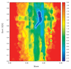
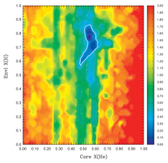
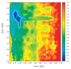
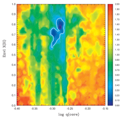
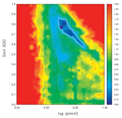
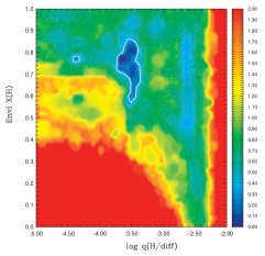
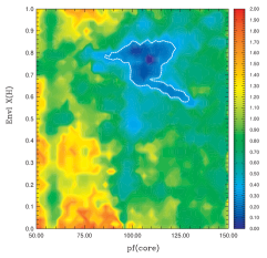
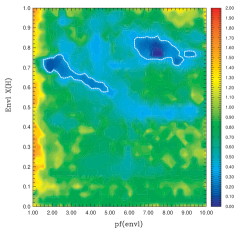
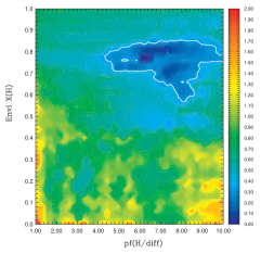
Figure 14: $\log S^{2}$-projection maps for pairs of model parameters showing location and shape of best-fit regions in parameter space (see Sect. 3.2 and text for details). All pairs include the $X({\rm H})_{{\rm envl}}$ parameter, thus showing correlations that may exist between this quantity and other model parameters. The quantity $S^{2}$ is normalized to one at minimum and the color scale is logarithmic. Dark blue indicates the best-fit regions and the dotted contour line is an estimate of the $1\sigma$ confidence level, obtained in a similar way to that described in Brassard et al. (2001).

The model parameter space searched for a best-fit seismic solution that matches the frequencies of TIC 278659026 was originally defined to cover the widest possible range assumed relevant for typical sdB stars. In this context, the quantity $X({\rm H})_{{\rm envl}}$, which sets the hydrogen mass fraction (and consequently the H/He mass ratio; see Fig.4) at the bottom of the envelope, was kept confined within a narrow range between 0.70 and 0.75, assuming that the main sequence progenitor probably had an H-rich envelope of roughly solar composition that remained unspoiled before reaching the hot sdB stage. However, the results from the seismic analysis suggests that TIC 278659026 has a relatively low mass and may not be a typical sdB star. This star may have undergone a nondegenerate ignition in the helium core, thus possibly originating from a massive progenitor. If produced, for instance, through a RLOF phase, the original composition of the envelope may have been altered to significantly differ from standard evolution expectations, where $X({\rm H})_{{\rm envl}}$ is possibly well outside the narrow range originally defined. Moreover, the lack of constraint from the seismic solution for this parameter in the 0.70 – 0.75 range (see Fig. 5 and 9) leaves open the possibility that a better seismic solution could reside outside of the parameter space originally searched.

To address this issue, we present additional computations extending the search to a much wider range of values for the $X({\rm H})_{{\rm envl}}$ parameter. A new optimization was launched within the ranges given in the third column of Table 2, except that $X({\rm H})_{{\rm envl}}$ was now allowed to vary between 0 and 1 (instead of 0.70 and 0.75 in the original search), thus covering the entire range of possible values for this parameter. Owing to the larger parameter space open for exploration, this calculation was performed on the high-performance cluster OLYMPE at the CALMIP computing center using 960 CPU cores in parallel, which ran for approximately two days and required the computation of 1,863,344 seismic models; thus this added to the 1,555,425 models already calculated in this study. The results are illustrated in Fig. 14.

First, we find no significant improvement in terms of quality of fit for the best solutions within this extended parameter space. The model formerly identified still holds up as among the best, i.e., within the $1\sigma$ contours shown in Fig. 14. Hence, no clear optimal value exists for $X({\rm H})_{{\rm envl}}$ that could have been missed because of the narrow range originally imposed. Instead, Fig. 14 reveals that best-fit models are found within a flat and elongated region that covers the range $X({\rm H})_{{\rm envl}}\sim 0.58-0.86$. Models with envelope hydrogen mass fractions above and below these limits appear to produce lower quality solutions. Therefore, a significantly helium-enriched envelope (with $Y\gtrsim 0.42$) for TIC 278659026 seems excluded.

The impact for the other model parameters of allowing a wider range of values for $X({\rm H})_{{\rm envl}}$ is limited (we refer again to Fig. 14). The best-fit stellar masses remain in the $\sim 0.375-0.40$ $M_{\odot}$ range, which is almost entirely contained in the errors quoted in Table 3 for this quantity. Interestingly, only models with $X({\rm H})_{{\rm envl}}\lesssim 0.62$ result in slightly lower mass solutions ($\lesssim 0.38$$M_{\odot}$), which arguably may be less consistent with other independent measurements for this quantity. Similarly agreeing with values and errors given in Table 3, the inferred helium and oxygen mass fractions in the core, $X({\rm He})_{{\rm core}}$ and $X({\rm O})_{{\rm core}}$, remain within the $0.48-0.62$ and $0.08-0.29$ ranges, respectively, while the core boundary fractional mass depth, $\log q({\rm core})$, is in the interval $[-0.31,-0.27]$. Slightly wider ranges for the main parameters defining the envelope structure are obtained. The best-fit fractional mass depth for the core-envelope boundary, $\log q({\rm envl})$, ranges from $-2.30$ to $-1.80$; there is a clear correlation with $X({\rm H})_{{\rm envl}}$ , i.e., less hydrogen is associated with a slightly deeper transition. The inferred location for the transition with pure-hydrogen layers, $\log q({\rm H/diff})$, is in the interval $[-3.70,-3.30]$.

We conclude from this extended search that the parameters derived from the original study restraining $X({\rm H})_{{\rm envl}}$ to the narrow interval $[0.70,0.75]$ are not fundamentally changed when widening this range. Therefore, the asteroseismic solution was not artificially constrained by this prior. The main impact, if we allow the H/He mass ratio to differ significantly from typical solar composition, is slightly larger uncertainties for some derived parameters.