A New Space Weather Tool for Identifying Eruptive Active Regions

Abstract

One of the main goals of solar physics is the timely identification of eruptive active regions. Space missions such as Solar Orbiter or future Space Weather forecasting missions would largely benefit from this achievement. Our aim is to produce a relatively simple technique that can provide real time indications or predictions that an active region will produce an eruption. We expand on the theoretical work of Pagano et al. (2019) that was able to distinguish eruptive from non-eruptive active regions. From this we introduce a new operational metric that uses a combination of observed line-of-sight magnetograms, 3D data-driven simulations and the projection of the 3D simulations forward in time. Results show that the new metric correctly distinguishes active regions as eruptive when observable signatures of eruption have been identified and as non-eruptive when there are no observable signatures of eruption. After successfully distinguishing eruptive from non-eruptive active regions we illustrate how this metric may be used in a “real-time” operational sense were three levels of warning are categorised. These categories are: high risk (red), medium risk (amber) and low risk (green) of eruption. Through considering individual cases we find that the separation into eruptive and non-eruptive active regions is more robust the longer the time series of observed magnetograms used to simulate the build up of magnetic stress and free magnetic energy within the active region. Finally, we conclude that this proof of concept study delivers promising results where the ability to categorise the risk of an eruption is a major achievement.

1 Introduction

The ability to identify eruptive active regions prior to an eruption is crucial for improving current space weather forecasting capabilities and to select targets for Solar Orbiter’s observing campaigns. The fundamental aim is to predict as early as possible the location of the source region that the next solar eruption will originate from and correspondingly the time of the eruption. Significant advances in this area have been made over the past few years due to the wealth of full disk data available from the Solar Dynamic Observatory (SDO). In particular, flare forecasting techniques have improved significantly. For a summary of state-of-the-art flare forecast models we refer readers to Barnes et al. (2016). To predict the occurrence of solar flares previous studies have accomplished this by examining either the active region properties from a physical perspective (Georgoulis & Rust, 2007; Kontogiannis et al., 2017; Jonas et al., 2018; Kontogiannis et al., 2018; McCloskey et al., 2018), or by using sophisticated computational techniques of data analysis (Ahmed et al., 2013; Bobra & Couvidat, 2015; Boucheron et al., 2015; Liu et al., 2017; Nishizuka et al., 2017; Raboonik et al., 2017; Nishizuka et al., 2018; Florios et al., 2018; Benvenuto et al., 2018; Liu et al., 2019; Domijan et al., 2019). However, increasing our capability of identifying flaring regions alone is currently not enough to improve space weather forecasting, as flares are only one component of eruptive solar activity. Space Weather events are largely produced by Coronal Mass Ejections (CMEs) that can be related to flares, but both phenomena can also occur without the other (Gopalswamy, 2004). Green et al. (2018) provides a thorough analysis of solar eruptions in relation to their predictability. A significant advancement in this area has been made by Murray et al. (2018) which has combined two large-scale projects to provide a crucial connection between the prediction of flares (FLARECAST Georgoulis et al., 2018) and how this can support the prediction of CMEs studied in the HELCATS catalogue (Bothmer et al., 2018). Also, Murray et al. (2017) illustrated an example of how agencies are preparing for operations of flare forecasts. In addition to flares, efforts have been deployed to predict the occurrence of CMEs, either using observable precursors (Baker et al., 2012), machine learning (Bobra & Ilonidis, 2016) or statistical approaches (Aggarwal et al., 2018).

In parallel to these studies, a large number of papers have significantly improved our understanding of the physical mechanisms that cause solar eruptions. While predictive techniques tend to empirically identify key parameters that are proxies of the eruption process, other studies identify what physical mechanisms trigger CMEs. Schmieder et al. (2015) and Green et al. (2018) provide recent overviews of the models of CMEs and flares, while Pagano et al. (2015) considers aspects related to numerical simulations. Very generally speaking, we can distinguish CME models in two main categories that describe how the Lorentz force imbalance that triggers the eruption is generated. We have MHD instability theories, where existing structures are in a metastable equilibrium, where the runaway from it can be catastrophic (Forbes & Isenberg, 1991), or it can follow either the Kink (Sakurai, 1976; Török & Kliem, 2005), or Torus (Kliem & Török, 2006; Démoulin & Aulanier, 2010; Aulanier et al., 2010) instability. Alternativelly, the force imbalance is generated by the removal of confining structures, such as in the Breakout model (Antiochos et al., 1999; Lynch et al., 2008). Morever, other eruption mechanims can be triggered outside or at the border of active regions, such as blowout jets (Chandra et al., 2017).

The aim of this paper is to provide a proof of concept study for a new approach to identify eruptive active regions based on the physical analysis provided by Pagano et al. (2019), which we will now refer to as Paper I. In Paper I, we analysed the 3D magnetic field evolution of a set of active regions using the magnetofrictional relaxation model of Mackay et al. (2011). We then derived a theoretical metric that discriminated eruptive from non-eruptive active regions. We identified an empirical threshold (based on the small sample of active regions considered) and we developed a magnetogram projection technique that allowed us to successfully apply the theoretical metric to both observed magnetograms and magnetograms projected forward in time. Building on Pagano et al. (2019), the goal of this paper is to develop a new operational metric that can be quickly computed and used to determine whether an active region is at risk of producing an eruption. In order to achieve this goal, we first determine the most suitable features in the time evolution of the theoretical metric that indicate the risk of an eruption and secondly we construct a method to summarise this analysis into a single value ranging from 0-1 that measures the risk of an active region producing an eruption.

The structure of the paper is as follows: in Sec.2 we summarise the data-driven magnetofrictional model used to simulate the 3D structure of the active regions, along with the main properties of the active regions used in this study. In Sec.3 we discuss a new approach in the application of projected magnetograms to predict the future time evolution of the active regions. Next in Sec.4 we present the practical application that classifies eruptive and non-eruptive active regions in the context of an operational model. In Sect.5 we draw conclusions and consider future advancements of the technique.

2 Summary of the model and simulations

To simulate the data-driven, 3D evolution of active regions we use the magnetofrictional relaxation model of Mackay et al. (2011). This technique uses a 3D cartesian domain where the initial coronal magnetic field is extrapolated from the first magnetogram in the time series evolution of the active region and is assumed to be potential. Next, the time sequence of observed line-of-sight magnetograms is applied as an evolving lower boundary condition where the evolution injects free magnetic energy and helicity into the coronal field. The coronal field then responds by evolving through a sequence of Nonlinear Force-Free states. As the initial condition is a potential field, we find that a ramp-up phase corresponding to approximately 35 magnetograms (2 days) is needed before the coronal magnetic field significantly departs from this initial configuration. After this time, the description of the active region magnetic field follows from the evolution of the applied line-of-sight magnetograms as it has lost its memory of the initial condition. Full details of the applied technique can be found in the papers of Mackay et al. (2011), Gibb et al. (2014), and Yardley et al. (2018b).

From the time series of the 3D magnetic field configurations for each active region, we derived a theoretical metric $\zeta\left(x,y,t\right)$ that can be used to distinguish eruptive from non-eruptive active regions, where $x$ and $y$ are the horizontal directions on the solar surface and $t$ is time. Full details regarding the computation of $\zeta\left(x,y,t\right)$ can be found in Section 3 of Paper I. However, in simple terms $\zeta\left(x,y,t\right)$ is the product of three different functions that are also normalised:

$$\zeta\left(x,y,t\right)=\omega\left(x,y,t\right)\mu\left(x,y,t\right)\sigma\left(x,y,t\right).$$ (1)

The terms composing $\zeta\left(x,y,t\right)$ are now described: (i) $\omega\left(x,y,t\right)$ is close to 1 at the location where a magnetic flux rope is present, (ii) $\mu\left(x,y,t\right)$ is close to 1 where the Lorentz force is directed outwards and (iii) $\sigma\left(x,y,t\right)$ is close to 1 where the Lorentz force is heterogeneous in space. In principle $\zeta\left(x,y,t\right)$ can take a value anywhere from 0-1 but in practise the value is found to be small with a strong spatial variation, In Paper I, we studied eight individual active regions, five of which were associated with an observed eruption and three which were not. Through considering the bi-dimensional time-dependent distribution of $\zeta\left(x,y,t\right)$ we extracted a time dependent quantity, $\zeta_{max}\left(t\right)$, i.e. the maximum of $\zeta\left(x,y,t\right)$ at each time that represents how the theoretical metric associated with an active region evolves in time. Furthermore, a single number $\bar{\zeta}$, that is the time average of $\zeta_{max}\left(t\right)$ over an extended period of time (hours to $\sim 1$ day), is able to distinguish between eruptive and non-eruptive active regions. Using our sample of active regions, we find an empirically derived threshold, $\bar{\zeta_{th}}=0.028$, for the value of $\bar{\zeta}$ that discriminates between the eruptive and non-eruptive active regions.

An important aspect considered in Paper I is that this metric remains useful in discriminating eruptive and non-eruptive active regions when we introduce projected magnetograms. Projected magnetograms were used to project the magnetic field evolution forward in time using the most recently available observed magnetograms. This was achieved by using the final two observed magnetograms to measure the electric field at the lower boundary of the 3D magnetofrictional simulation, as a function of space $(x,y)$ assuming it was constant thereafter, throughout the time of the projection. In Paper I, we ran a set of simulations where we replace observed magnetograms with projected ones and found that the metric $\bar{\zeta}$ is not significantly altered when enough observed magnetograms are used prior to the projection.

In the present paper, we develop a practical application of the theoretical approach presented in Paper I that illustrates the possible operational use of this technique. In this application, we test the possibility of using the data-driven magnetofrictional simulations of Mackay et al. (2011) combined with the metrics identified in Paper I for the continuous monitoring of active regions. We illustrate how the technique could be used to issue warnings of the risk of eruptions when the observed and forecasted magnetic field configurations produce values of $\bar{\zeta}$ above a critical value. To carry out this application we use a mixture of observed magnetograms and projected magnetograms over a limited time period. A key new aspect of the present paper, compared to the technique used in Paper I is that, (i) here we use projected magnetograms for a fixed time span only and (ii) we introduce a more advanced measure to quantify the risk for an active region to produce an eruption. This advanced metric builds in more information from the active region evolution compared to that used in Paper 1 and develops the theoretical metric into an operational context. The work-flow of the technique is a follows:

• We first run a set of magnetofrictional simulations where we vary the time when we switch from observed to projected magnetograms.

• Next, we derive a function from the theoretical metric $\zeta\left(x,y,t\right)$ that measures how the metric changes between the projected and observed evolution and how it relates to the empirical threshold identified in Paper I.

• Based on this new metric we classify the state of the active region at a given time as either, red $\sim$ high risk, amber $\sim$ medium risk or green $\sim$ low risk to serve as a warning for potential forthcoming eruptions.

A key element of this study is the selection of active regions used to present the new technique. Full details of the active regions can be found in Paper I and Yardley et al. (2018b, a, 2019) where Table1 presents the main properties of the active regions. The technique applied in this paper is applicable to all types of active region. However, for the present study, we have focused on an initial small sample of young isolated active regions as this allows us to capture the full evolution of the active region (from birth to decay) in the NLFFF simulations. The magnetic field evolution of the active regions under consideration can then be analysed using the metric that is based only on the magnetic field properties and its time evolution. In principle, any model that accurately reproduces the magnetic field configuration and evolution of the active region can be used to apply this metric, even if some technical difficulties might need to be overcome. Examples of potential technical challenges that need to be overcome in terms of the NLFFF model, such that arbitrary active regions can be studied are: i) maintaining a high spatial resolution over large fields of view, ii) modelling active regions that have merged and undergone significant evolution and the injection of non-potentiality and iii) non-localised active regions where the equilibrium is perturbed by eruptions occurring elsewhere. In the future we will refine the NLFFF model used in the proof of concept study carried out here to tackle these challenges.

Table 1: Active region properties, as in Pagano et al. (2019). These active regions have been previously studied by Rodkin et al. (2017), James et al. (2018), Yardley et al. (2018b), Yardley et al. (2018a), Yardley et al. (2019).

Active region	Observation Start	Observation End	Magnetogram cadence	Eruption at	Publication
AR11561	2012.08.29 19:12:05	2012.09.02 01:36:04	96 min	2012.09.01 23:37	Yardley+2018b, 2019
AR11680	2013.02.24 14:23:55	2013.03.03 19:11:56	96 min	2013.03.03 17:27	Yardley+2018b, 2019
AR11437	2012.03.16 12:47:57	2012.03.21 01:35:58	96 min	2012.03.20 14:46	Yardley+2018a,b, 2019
AR11261	2011.07.31 05:00:41	2011.08.02 06:00:41	60 min	2011.08.02 05:54	Rodkin+2017
AR11504	2012.06.11 00:00:08	2012.06.14 22:24:08	96 min	2012.06.14 13:52	James+2018
AR11480	2012.05.09 11:12:05	2012.05.14 00:00:05	96 min	none	Yardley+2018b, 2019
AR11813	2013.08.06 01:36:07	2013.08.12 00:00:07	96 min	none	Yardley+2018b, 2019
AR12455	2015.11.13 04:47:55	2015.11.18 23:59:54	96 min	none	Yardley+2018b, 2019

3 Rolling projection of the eruption metric

In Paper I, we have shown that through studying the evolution of the 3D configuration of the magnetic field of an active region it is possible to distinguish eruptive from non-eruptive active regions. We also concluded that the introduced theoretical metric was robust in identifying eruptive active regions when we use projected magnetograms as part of the time sequence instead of observed magnetograms. In this section, we address whether the same modelling technique can be used with a rolling projection time corresponding to 10 magnetograms and how the metric derived from these simulations can be used to identify eruptive active regions. We note that the 10 magnetograms represents either a projection time of $\sim 10$ $hrs$ or $\sim 16$ $hrs$ depending on whether the cadence of the magnetograms, $\Delta t$, is 60 or 96 minutes).

To implement the rolling projection we define $t_{0}$ as the start time when we switch from observed to projected magnetograms. The value of $t_{0}$ must lie between the first and final observed magnetogram and, in practical terms, we vary $t_{0}$ such that in successive simulations more observed magnetograms are used prior to the period of projection. This reproduces the situation of observing an active region up to a given time, $t_{0}$ and then projecting its evolution forward in time. From the time $t_{0}$ we then run the 3D magnetofrictional simulation forward for a time period equivalent to the acquisition of 10 magnetograms, i.e. until the time $t=t_{0}+10\Delta t$. The final time of the projected simulations may be either before or after the time of the last observed magnetogram in our time series given in Tab.1 depending on when the projection starts. For these projected simulations we compute $\bar{\zeta}$ by averaging the value of $\zeta_{max}\left(t\right)$ over only the time span of the 10 projected magnetograms. This method of computing $\bar{\zeta}$ is different from that used in Paper I, as it is now only computed during the projected interval. In our study we start from a value of $t_{0}$ that is at the end of the ramp-up phase i.e. the initial phase during which the magnetic field loses memory of its initial potential configuration. To implement the rolling nature of the simulations after each period of projection we return and increase $t_{0}$ by $\Delta t$ through using another observed magnetogram before carrying out another projection. This process is repeated until we reach the time $t_{f}$ of the final magnetogram in the observation time series. In a real application, this study corresponds to starting from an initial time series of magnetogram observations and as soon as more observational information becomes available, $t_{0}$ is increased by $\Delta t$, and the projection is repeated after the observed evolution is updated using the most recent measurements. Such a technique, where our simulations temporal window moves can be used to determine whether the $\bar{\zeta}$ associated with an active region is going to be above or below the threshold for eruptions and whether it will increase or decrease. In an operational sense, this will partially address the question of whether an eruption is becoming more or less likely.

Fig.1 considers the value of $\bar{\zeta}$ obtained in these projected simulations (blue asterisks) as a function of $t_{0}$, shown for the eruptive active regions. In each plot the black curve gives the variation of the maximum of $\zeta\left(x,y,t\right)$, deduced from Paper I (defined as $\zeta_{max}\left(t\right)$) when only observed magnetograms are used. The black line is split into two segments where the black dashes are during the ramp-up phase of the magnetofrictional simulation and solid black line after the ramp-up phase. In each plot the solid magenta line denotes the time of the observed eruption, $t_{e}$, where the plots are normalised with respect to $t_{e}$, such that $(t_{0}-t_{e})/\Delta t=0$. The dashed magenta line denotes the time, $(t_{0}-t_{e})/\Delta t=-10$, such that the end time of the projected simulation occurs at the time of the eruption $t_{e}$. In general the quantity $\bar{\zeta}$ determined for the projected magnetograms is larger than the value of $\zeta_{max}\left(t\right)$ obtained from the full observational data set. We now consider the evolution of $\bar{\zeta}$ and compare them with $\zeta_{max}\left(t\right)$ for each individual active region.

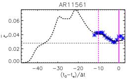
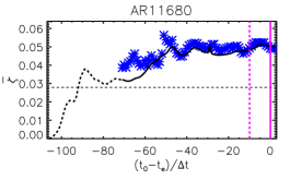
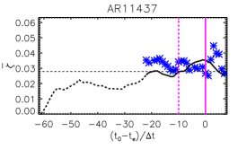
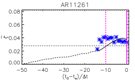
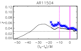
Figure 1: The black line represents the evolution of $\zeta_{max}\left(t\right)$ for the eruptive active regions. Blue asterisks at each $t_{0}-t_{e}/\Delta t$ are the values of $\bar{\zeta}$ obtained from the simulation that ran for 10 projected magnetograms after the observed one at $t_{0}$. The magenta vertical lines represent the time of eruption, $t_{e}$ (continuous) and $t_{0}-t_{e}=-10\Delta t$ (dashed). The horizontal dashed black line represents the value of $\bar{\zeta_{th}}=0.028$.

For AR11561 care must be taken, as we start using projected magnetograms immediately after the end of the ramp-up phase of the magnetofrictional simulation. Due to this it has the least amount of prescribed observational evolution prior to the start of the projections. The value of $\bar{\zeta}$ at $(t_{0}-t_{e})/\Delta t=-10$ is slightly larger than the value of $\zeta_{max}\left(t\right)$ at the same time. Both quantities initially decrease in value, however they start to increase again shortly before the time of the observed eruption. While all the values of $\bar{\zeta}$ remain above the indicated threshold, $\zeta_{th}$, it is difficult here to identify a precise time when the active region becomes eruptive from the projected simulation. However, the active region is classified as eruptive throughout the entire projected time period.

As we already discussed in Paper I, AR11680 is an active region that remains classified as eruptive for a significant period of time, as it consistently shows high values of $\zeta_{max}\left(t\right)$. Over the time period of $-70<(t_{0}-t_{e})/\Delta t<-50$ the projected magnetogram simulations show an increasing value of $\bar{\zeta}$. During this time period, $\zeta_{max}\left(t\right)$ also increases and the values of $\bar{\zeta}$ and $\zeta_{max}\left(t\right)$ plateau together. In this case, the only plausible conclusion is that an eruption is likely anytime after $\bar{\zeta}$ plateaus.

For AR11437, just after the ramp-up phase there is a significant difference between $\bar{\zeta}$ and $\zeta_{max}\left(t\right)$. The estimated value of $\bar{\zeta}$ then converges towards the value of $\zeta_{max}\left(t\right)$. Near $(t_{0}-t_{e})/\Delta t=-10$ the value of $\bar{\zeta}$ increases sharply to a value similar to that found for $\zeta_{max}\left(t\right)$ at the eruption time $(t_{0}-t_{e})/\Delta t=0$. Then, the value of $\bar{\zeta}$ decreases after $(t_{0}-t_{e})/\Delta t=-10$, in the same way as $\zeta_{max}\left(t\right)$ does after the eruption time $(t_{0}-t_{e})/\Delta t=0$. The fact that the evolution of $\bar{\zeta}$ about $(t_{0}-t_{e})/\Delta t=-10$ resembles that found for $\zeta_{max}\left(t\right)$ about $(t_{0}-t_{e})/\Delta t=0$, is a remarkable result for the magnetogram projection technique. Additionally, in Paper I a decline in $\zeta_{max}\left(t\right)$ was explained by the occurrence of an eruption, after which the magnetic field releases free energy and evolves to a simpler configuration. This simpler configuration is naturally associated with smaller values of $\zeta\left(x,y,t\right)$.

For AR11261 the magnetogram time series is probably too short to produce conclusive results. At $(t_{0}-t_{e})/\Delta t=-10$ we find values of $\bar{\zeta}$ that are much larger than those found for $\zeta_{max}\left(t\right)$. This can be attributed to one of two reasons. It could be related to the occurrence of the eruption that follows shortly afterwards or it could be due to the overestimation in $\bar{\zeta}$ that tends to occur just after the ramp-up phase. However, this active region would also be characterised as eruptive.

Finally, AR11504 shows a behaviour similar to AR11437 where the values of $\bar{\zeta}$ are larger than $\zeta_{max}\left(t\right)$ after the ramp-up phase. This is followed by an increase in the value of $\bar{\zeta}$ near $(t_{0}-t_{e})/\Delta t=-10$ which is a signature of the eruption. Afterwards, the value of $\bar{\zeta}$ converges towards the value of $\zeta_{max}\left(t\right)$ where both steadily decrease.

We also apply this technique to the non-eruptive active regions where the results can be seen in Fig.2. As these active regions do not have any observed eruptions the results are presented with respect to the time of the final observed magnetogram, $t_{f}$. We find that for AR11480 the estimations of $\bar{\zeta}$ converge to a value under the threshold and therefore it would be classified as non-eruptive. For AR11813 the value of $\bar{\zeta}$ is initially very high after the ramp-up phase, but it converges to be below the threshold. Thus while during the early part of the projected evolution it would be classified as eruptive, for the later stages it would be non-eruptive. Finally, AR12455 presents a very oscillatory behaviour for both $\zeta_{max}\left(t\right)$ and $\bar{\zeta}$, where both values oscillate above and below the threshold. The amplitude of the oscillations decay and near the end the values sit below the threshold.

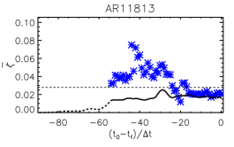
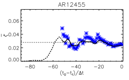
Figure 2: The black line represents the evolution of $\zeta_{max}\left(t\right)$ for the non-eruptive active regions. Blue asterisks at each $t_{0}-t_{e}/\Delta t$ are the values of $\bar{\zeta}$ obtained from the simulation that ran for 10 projected magnetograms past the observed one at $t_{0}$. The horizontal dashed black line represents the value of $\bar{\zeta_{th}}=0.028$.

All projected simulations show a value of $\bar{\zeta}$ that converges to a value that is larger/smaller than the empirical threshold $\bar{\zeta_{th}}$ (dashed line), for the eruptive/non-eruptive active regions respectively. Thus the value of $\bar{\zeta}$ can discriminate between eruptive and non-eruptive active regions over a prediction time period of $\sim 10$ magnetograms (10-16 hrs).

In summary, for eruptive active regions we find that the projected evolution of $\bar{\zeta}$ is consistently larger than the empirical threshold $\zeta_{th}$ that we have identified in Paper I. This means that many of these active regions would be classified as eruptive. While this is the case, the technique cannot currently provide an indication of the time of the eruption, and more work is needed in future to determine this. For the non-eruptive active regions the projected values of $\bar{\zeta}$ can be highly scattered directly after the ramp-up phase, e.g. when the projection technique overestimates the effect of flux emergence. During this early stage the non-eruptive active regions may be initially classified as eruptive, but as the evolution proceeds, the value of $\bar{\zeta}$ falls below the threshold and the active regions would be classified as non-eruptive. With the presently used theoretical metric the distinction of eruptive and non-eruptive active region remains over a rolling projection time for this small sample study. However, the values of the parameters found are subtle. Therefore in the next section we aim to improve this metric into an operational framework by including more information such that we can more clearly distinguish eruptive and non-eruptive active regions.

4 An Operational Metric for Predicting eruptive active regions.

In this section, we develop a new method based on the theoretical method introduced in Sec.3. This new method will be more suitable to apply operationally. The aim of this operational metric is to provide a measure of the eruptive condition of an active region at a given time $t_{0}$, where we run the magnetofrictional simulations using observed magnetograms until $t_{0}$ and projected ones after $t_{0}$ until $t_{0}+10\Delta t$ (10 $\sim$ 16 hrs). Our results from Paper I (where we used only observed magnetograms or a long series of projected ones) and from Sec.3 (where we used a limited series of projected magnetograms) clearly show that our theoretical metric $\bar{\zeta}$ discriminates between eruptive and non-eruptive active regions. At the same time, an ad-hoc analysis was required to correctly interpret the results of the metric from the magnetofrictional simulations as the interpretation could be subtle. For instance, we learned that i) we need to discard information obtained too close to the end of the ramp-up phase, ii) the theoretical metric naturally tends to decrease in the aftermath of an eruption and iii) we need to compare the value of the metric with our empirical threshold in addition to its previous values. To carry out this analysis manually in an operational context is not entirely realistic, as we need the assessment to be carried out automatically by machines. Therefore, there is the need for a new operational metric to be introduced that encompasses the analysis given in Sect.3 into one simple indicative number that measures the risk that an active region is going to produce an eruption or not.

The operational metric is defined by the function $\Lambda$ that depends on the past evolution, present configuration and projected evolution of the active region. More specifically, it depends on values of $\bar{\zeta}$ when $\zeta_{max}\left(t\right)$ is averaged over different time windows, the instantaneous value of $\zeta_{max}\left(t\right)$, and the time derivative of $\zeta_{max}\left(t\right)$. In the next section we outline how we derive the value of $\Lambda$.

4.1 Computation of $\Lambda$

To compute $\Lambda$ we use the following definitions:

• $\zeta_{max}\left(t\right)$: the maximum value of $\zeta\left(x,y,t\right)$ at any given time t.

• $\bar{\zeta}_{+10}$: the value of $\bar{\zeta}$ averaging $\zeta_{max}\left(t\right)$ over the time period $10\Delta t$ from $t=t_{0}$ (using only projected magnetograms).

• $\bar{\zeta}_{-10}$: the value of $\bar{\zeta}$ averaging $\zeta_{max}\left(t\right)$ over the time period $10\Delta t$ until $t=t_{0}$ (using only observed magnetograms).

• $\delta\zeta=\frac{\zeta_{max}\left(t\right)-\zeta_{max}\left(t-2\Delta t\right)}{2}$: the rate of change of $\zeta_{max}\left(t\right)$ between the magnetograms at $t=t_{0}$ and $t=t_{0}-2\Delta t$.

Using these quantities we next define a set of arctan functions $\alpha$, that can have values ranging from 0 to 1,

$$\alpha_{\zeta+10}=\frac{1}{\pi}\arctan\left(\frac{\bar{\zeta}_{+10}-\left(\bar{\zeta_{th}}+\beta_{th}\right)}{\beta_{th}}\right)+\frac{1}{2}$$ (2)

$$\alpha_{\zeta}=\frac{1}{\pi}\arctan\left(\frac{\zeta_{max}\left(t\right)-\left(\bar{\zeta_{th}}+\beta_{th}\right)}{\beta_{th}}\right)+\frac{1}{2}$$ (3)

$$\alpha_{+10-10}=\frac{1}{\pi}\arctan\left(\frac{\bar{\zeta}_{+10}-\bar{\zeta}_{-10}}{\beta_{+10-10}}\right)+\frac{1}{2}$$ (4)

$$\alpha_{n}=\frac{1}{\pi}\arctan\left(\frac{n-n_{ramp-up}}{0.5}\right)+\frac{1}{2}$$ (5)

where $n$ is the magnetogram index, $n_{ramp-up}$ is the last magnetogram in the ramp-up phase, $\beta_{th}$ and $\beta_{+10-10}$ are parameters that determine where and how steeply each $\alpha$ function transitions from values close to 0, to values close to 1. In our application we use the following values for these parameters, $\beta_{th}=\beta_{+10-10}=10^{-4}$ and $n_{ramp-up}=35$. The latter value is chosen to be 35, as in Paper I we state that the 35th magnetogram of each sequence is the end of the ramp-up phase.

The rationale of the $\alpha$ functions is the following. Values of $\alpha_{\zeta+10}$ close to 1 lead to a higher eruption risk. This happens when the value of $\bar{\zeta}_{+10}$ is larger than the threshold $\bar{\zeta_{th}}$, which means that the active region is going to be in an eruptive state according to the magnetic field evolution predicted by the projected magnetograms. The same applies to $\alpha_{\zeta}$ that depends on how the instantaneous value of $\zeta_{max}\left(t\right)$ relates to the same threshold $\bar{\zeta_{th}}$. Values of $\alpha_{+10-10}$ close to 1 also indicate an increased risk of eruption and are found when $\bar{\zeta}_{+10}$ is larger than $\bar{\zeta}_{-10}$. This happens when the projected magnetograms predict that the active region is going to be more likely to erupt, compared to what is measured in the evolution of the prior 10 observed magnetograms. Therefore $\alpha_{+10-10}$ measures the long term time variation of the metric over the time span corresponding to 20 magnetograms. Finally, $\alpha_{n}$ takes values close to 1 when the time $t_{0}$ is far from the ramp-up phase of the magnetofrictional simulations. This is to mitigate the impact of high values of $\bar{\zeta}_{-10}$, due to the ramp-up phase giving false positives.

Finally, we also use another $\alpha$ function that gives negative values, between -1 and 0

$$\alpha_{\Delta\zeta}=\frac{1}{\pi}\arctan\left(\frac{\delta\zeta}{\beta_{\Delta\zeta}}\right)-\frac{1}{2}.$$ (6)

where $\beta_{\Delta\zeta}=10^{-3}$, This function measures the short term time variation of the metric over the time span of 2 magnetograms and has values close to -1 when the value of $\zeta_{max}\left(t\right)$ drops. This helps identify times immediately after an eruption has occurred where the risk of another one is reduced.

These parameter values ($\beta_{th}$, $\beta_{+10-10}$, and $\beta_{\Delta\zeta}$) have been chosen such that the $\alpha$ functions switch from 0 to 1 within the range of values encountered for $\bar{\zeta}_{+10}$, $\bar{\zeta}_{-10}$, and $\zeta_{max}\left(t\right)$ in this present small sample study using young active regions. Finally, we weight the $\alpha$ functions with $w_{+10-10}=1$, $w_{\zeta+10}=4$, $w_{\zeta}=4$, $w_{\Delta\zeta}=1$ and we compute $\Lambda$ as

$$\Lambda=\frac{w_{+10-10}\alpha_{+10-10}\alpha_{n}+w_{\zeta+10}\alpha_{\zeta+10}+w_{\zeta}\alpha_{\zeta}+w_{\Delta\zeta}\alpha_{\Delta\zeta}}{w_{+10-10}+w_{\zeta+10}+w_{\zeta}+w_{\Delta\zeta}}.$$ (7)

It should be noted that only the function $\alpha_{+10-10}$ is multiplied by $\alpha_{n}$, as it is the only $\alpha$ function that depends on values of the metric at times before $t_{0}$ and thus can be affected by the magnetic field description during the ramp-up phase. In this work, the values for the weight parameters $w_{+10-10}$, $w_{\zeta+10}$, $w_{\zeta}$, $w_{\Delta\zeta}$ have been chosen after a number of tests in order to best associate higher values of $\Lambda$ with active regions that are observed to erupt and, more specifically, with the time $t_{0}$ falling within $t_{e}-10\Delta t<t_{0}<t_{e}$. While the qualitative contribution of each $\alpha$ function to $\Lambda$ is physically motivated and deduced from the properties of the metric $\bar{\zeta}$ defined in Paper I, the quantitative parameters used in each may still need to be refined. In this preliminary study we have selected by trial and error a set of parameters and weights for the $\alpha$ functions that return high risk of eruption for the eruptive active regions in the time period before the observed eruptions and low risk of eruption outside of this time period or for non-eruptive active regions. We note that it is possible to find unique values of parameters and weights that give consistent results for all the 8 active regions considered. However, care must be taken in the analysis of larger AR samples that contain a wider range of active regions as these values may depend on the stage of their evolution or vary with different types of active region. Finally, with this new operational metric defined by $\Lambda$ we expect active regions to fall in the full range of values from 0-1.

4.2 Operational Application of $\Lambda$

To be able to use the function $\Lambda$ for an operational application, we empirically define two thresholds to quantify when an active region is entering an eruptive state. We consider that an eruption is likely (eruptive active region) when $\Lambda\geq 0.55$, it is not likely (non-eruptive active region) when $\Lambda<0.35$, and the active region is borderline eruptive in the range $0.35<\Lambda\leq 0.55$.

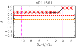
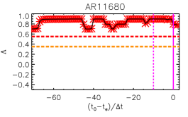
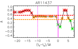
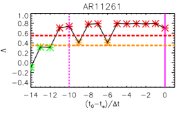
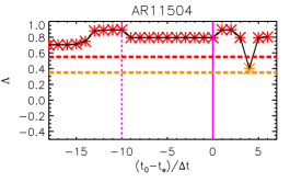
Figure 3: The evolution of $\Lambda$ for the eruptive active regions as a function of $t_{0}$ (black line). The asterisk symbols at each $t_{0}-t_{e}/\Delta t$ are the values of $\Lambda$ for each simulation with a given $t_{0}$. Symbols are red for $\Lambda\geq 0.55$, amber for $0.35\geq\Lambda<0.55$, and green for $\Lambda<0.35$. The amber and red dashed horizontal lines represent these thresholds, respectively amber and red. The magenta vertical lines represent $t_{e}$ (continuous) and $t-t_{e}=-10\Delta t$ (dashed).

Fig.3 shows the evolution of the value of $\Lambda$ (asterisks) as a function of $\left(t_{0}-t_{e}\right)/\Delta t$ for the active regions which were associated with observed eruptions. The asterisks are colour coded such that they are: red when $\Lambda\geq 0.55$, amber when $0.35\leq\Lambda<0.55$, and green when $\Lambda<0.35$. The solid magenta line represents the time of the observed eruption. While the dashed magenta line gives the time $t_{0}=t_{f}-10\Delta t$ where the first projected simulation includes the observed eruption within its projected time span. These plots show only the time interval after the ramp-up phase of each simulation.

The ideal outcome is that all of the asterisks in the interval between the dashed and continuous magenta lines are red or amber, and that the asterisks are green outside of this interval. However, this is not the case and so while this technique is useful in identifying eruptive active regions, it needs improvement to address the exact time window of the eruption within the active regions. AR11561 and AR11680 show high values of $\Lambda$ at all times and are thus considered eruptive at all times. Similarly, AR11504 is considered eruptive for the vast majority of the time, except near the end of the magnetogram time series where a decrease of $\alpha_{\Delta\zeta}$ reduces the value of $\Lambda$ after the time of the observed eruption. AR11437 shows mixed results where the active region appears eruptive for $t_{0}<t_{e}-10\Delta t$ and then it decreases to an amber alert in the time frame before the observed eruption. However, it immediately decreases to a non-eruptive classification after the eruption, with the exception of a couple of points. AR11261 shows a rather successful classification, as it is initially categorised as non-eruptive for $t_{0}<t_{e}-12\Delta t$ and then it increases to a red or amber alert during the time period when the active region is expected to be eruptive. From these results it can be seen that in 4 out of the 5 active regions $\Lambda$ successfully measures the risk of eruption in the active regions for the time periods leading up to the observed eruption. For the remain active region it would be borderline eruptive.

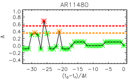
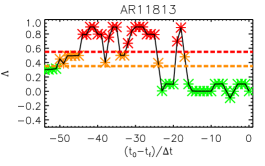
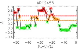
Figure 4: The evolution of $\Lambda$ for the non-eruptive active regions as a function of $t_{0}$ (black line). The asterisk symbols at each $t_{0}-t_{e}/\Delta t$ are the values of $\Lambda$ for each simulation with a given $t_{0}$. Symbols are red for $\Lambda\geq 0.55$, amber for $0.35\geq\Lambda<0.55$, and green for $\Lambda<0.35$. The amber and red dashed horizontal lines represent these thresholds, respectively amber and red.

Fig.4 shows the evolution of $\Lambda$ for the non-eruptive active regions, where we also find promising results. A common feature of each plot is that the initial values of $\Lambda$, obtained during the early projection simulations just after the ramp-up phase, are rather scattered. In contrast, as the simulations progress and more observational information is incorporated, the values of $\Lambda$ settle to values less than 0.35, where the active regions are correctly classified as non-eruptive during these times. In Paper I, we had already found a similar feature, where the magnetofrictional simulation description of the 3D magnetic field configuration becomes increasingly more accurate as we depart from the ramp-up phase.

5 Conclusions

In this paper, we have extended the theoretical study of Paper I towards a possible practical application that aims to monitor active regions and identify which ones are more likely to produce an eruption. In particular, we use the same set of active regions as in Paper I (5 eruptive and 3 non-eruptive) and simulate their 3D magnetic field evolution with a data-driven magnetofrictional model. To obtain the future risk of eruptions we develop a technique that uses a combination of observed and projected magnetograms as the lower boundary condition. We then apply the metric, $\bar{\zeta}$, that we have introduced in Paper I to verify that it can discriminate between eruptive and non-eruptive active regions when using projected magnetograms over a fixed time period of around 10 magnetograms (10-16hrs). The metric is based on three properties of the magnetic field that are linked to eruptions: the presence of magnetic flux ropes, the strength and direction of the Lorentz force and finally the Lorentz force heterogeneity. In this paper, we use the metric $\zeta\left(x,y,t\right)$ and quantities derived from it, such as $\zeta_{max}\left(t\right)$ and $\bar{\zeta}$, to define a new parameter $\Lambda$ that, in this exploratory study is applied to the same set of active region as in Paper I. We show that $\Lambda$ more clearly predicts the risk of an eruption in the next 10 to 16 hours (approximately 10 magnetograms at the cadence used in this work).

The parameter $\Lambda$ is constructed using a combination of quantities derived from $\zeta\left(x,y,t\right)$ and its value cannot exceed 1 by construction. In our study we find values in the full range from 0-1 and we identify two empirical operational thresholds for $\Lambda$. When $\Lambda\geq 0.55$ there is a high risk that the active region will produce and eruption (red alert), when $\Lambda<0.35$ the risk is instead rather low (green alert). We also identify a medium risk when the value of $\Lambda$ is between the thresholds (amber alert). We find that in some cases we have clear indications of an eruption becoming more likely as the value of $\Lambda$ exceeds the thresholds that we have empirically identified. From the point of view of simple identification of eruptive active regions, the technique clearly reaches its goal, as all five eruptive active regions are classified as eruptive for the majority of the simulated active region evolution. Additionally, our technique classifies some of the eruptive active regions as non-eruptive when the evolution is still far from the eruption time or post-eruption, thus limiting false positives. One limitation of the present technique is that it cannot yet identify the exact eruption time of a specific eruption. In the near future we hope to overcome this by improving the derivation of the metrics $\zeta\left(x,y,t\right)$ and $\Lambda$ along with their practical applications. We note that this initial specification of the threshold may need to be revised when the sample of active regions considered is increased.

Presently, it remains to be determined whether a prediction of the eruption time is possible at all with the spatial resolution of the current instruments. The elusive nature of the eruption time can be a consequence of the sensitive nature of the mechanisms that trigger solar eruptions. If it is so, it is natural that active regions remain in a metastable equilibrium for a long time before something at smaller spatial scale or some external trigger causes the runaway from equilibrium and the eruption. If this is the scenario we are facing, identifying eruptive active regions is the only achievable goal for the next few decades until new instruments allow us to resolve the dynamics at smaller spatial scales.

We also find that non-eruptive active regions are generally associated with low values of $\Lambda$ when $t_{0}$ is far enough from the end of the ramp-up phase, providing a correct classification. In contrast, a higher number of false positives are found near the end of the ramp-up phase in the simulation. This phase corresponds to the time required for the simulations to depart from the initial potential magnetic configuration that we know to be an inaccurate representation of the active region magnetic field. We have already stressed in Paper I and in other works how crucial it is to have a long time series of magnetograms in order to reach a satisfactory detailed description of the magnetic field in the active region. Therefore, we believe that these uncertainties can be reduced if longer time series of magnetograms are available, as we have shown in Paper I. In Paper I, it was also shown that the projection simulations perform better in reproducing the value of $\bar{\zeta}$ for the active regions where we have a longer time series available. To mitigate this problem, the best approach would be to develop the code so that the initial field condition is constructed from an NLFFF extrapolation based on a vector magnetogram. In the future, we intend to develop such a capability, which would allow extended testing on a wider sample of active regions, whose observations start days or weeks after they have emerged.

To put our work in context, the forecasting of solar eruptions is a topic that has attracted great interest in recent years (Huang et al., 2018; Laurenza et al., 2018; Leka et al., 2018; Liu et al., 2017; Nishizuka et al., 2018; Korsós et al., 2015; Kontogiannis et al., 2017, 2018). One of the most promising efforts has been made by the EU Flare Likelihood and Region Eruption Forecasting project (FLARECAST; Georgoulis et al., 2017) that associate a number of features readily measurable from active region observations to the likelihood that an eruption will occur. These studies have generally connected properties derived from observed magnetograms to some likelihood of eruption. However, the 3D magnetic field which is analysed in our paper inherently carries more information about the stability of the coronal structures than photospheric observations alone. Existing NLFFF models, in particular the magnetofrictional model, allow computationally fast continuous simulations of the full 3D magnetic field, and the prediction obtained from this approach can be more detailed. The initial work presented in Paper 1 and the present paper provides a pathway for future research focused on developing a robust model to predict active region eruptions. Here we have adopted the simplest approach in terms of the metric and projection technique, but we have nevertheless explored the possibility of identifying eruptive from non-eruptive active regions.

For a more practical perspective, we propose that in the future that this technique will be able to run automatically on space weather systems that focus on active regions monitoring. We imagine that our framework, the St Andrews Space Weather Active Region Monitor (S²WARM), is particularly useful for issuing timely space weather warnings or supporting scientific missions and their target selection for observation campaigns . Fig.5 and the corresponding movies available online show an example of how the technique can be implemented in a visual interface, where we simultaneously show the most recently available magnetogram of the active region at $t=t_{0}$ (upper left panel), the projected distribution of $\zeta\left(x,y,t\right)$ for $t>t_{0}$ (upper right panel) and the evolution of $\Lambda$ (lower panel). The panels are updated as new magnetogram observations and predictions are acquired. This framework allows for a constant monitoring of the active regions present on the solar disk and can facilitate decisions in space weather or mission control centres.

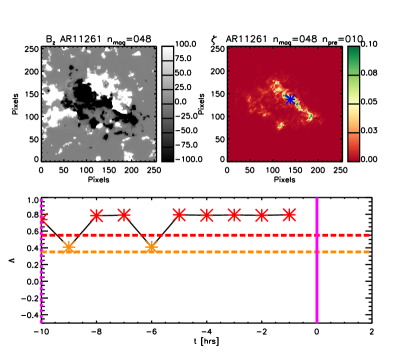
Figure 5: Example of graphic interface for S²WARM (movies available online). The top panels are used to represent the most updated observed magnetogram (left) and the projected distribution of $\zeta\left(x,y,t\right)$ (right), respectively. The lower panel shows the evolution of $\Lambda$ at the time of the most recent magnetogram. In this example for AR11261, we show the magenta lines that represent the time of the eruption (continuous line) and the time of 10 magntograms before the eruption (dashed line), i.e. when the technique should start identifying the active region as erupive.

Naturally, it is expected that our framework is going to be benchmarked against already existing space weather predictive tools. For instance, forecasting tools such as MAG4 (Falconer et al., 2011, 2014) that is used by the National Oceanic and Atmospheric Administration (NOAA) and by NASA’s Space Radiation Analysis Group (SRAG) and the FLARECAST (Georgoulis et al., 2017, 2018) platform that is developed by a consortium of European based institutions and includes some follow up applications using machine learning (Florios et al., 2018). The direct comparison between these approaches can significantly empower our capacity of responding to Space Weather hazards.

Despite the present technique not being currently able to predict the eruption time, it does open new opportunities to give more advanced warnings through the coupling of space weather models to the low solar corona. A number of space weather forecasting tools, such as EUPHORIA (Pomoell & Poedts, 2018), or WSA-ENLIL (Arge & Pizzo, 2000; Odstrcil, 2003) rely on the cone model (Xie et al., 2004). The cone model is a simplified description of the injection of CMEs into the solar wind. The combination of the magnetofrictional relaxation technique along with the method of projected evolution allows us to identify eruptive active regions and then run tentative space weather forecast simulations prior to the eruption with different speculated eruption times to have broad predictions on the trajectory, speed, and properties of the Interplanetary CME (ICME). Also, running successive magnetofrictional simulations, as more observational data is acquired, will allow us to reduce the uncertainties in the predicted ICMEs properties. In a more complex scenario, it is possible to couple the results of this approach with full MHD simulations of the low solar corona as in Pagano et al. (2013), Rodkin et al. (2017), and Pagano et al. (2018) to produce a more realistic insertion model of the CME into the solar wind. This more realistic model could include the time evolution of the magnetic field vectors along with the mass and velocity of the ejected material.

Finally, it should be mentioned that this work is fundamentally based on the analysis of a series of 3D magnetic field configurations of active regions. Starting from the previous works where the magnetofrictional model generates an accurate representation of the 3D magnetic field configuration, we have then been guided by the physical interpretation of the results to derive $\zeta\left(x,y,t\right)$, $\zeta_{max}\left(t\right)$, $\bar{\zeta}$, and finally the prediction parameter $\Lambda$. An alternative route that we have not explored yet is to use machine learning techniques in order to extract different proxies from the 3D configuration of the magnetic field that may outperform our current technique. We have thus far preferred a physics-minded approach, as our goal is not only the practical application of this study for the benefit of space weather predictions and Solar Orbiter operations, but also a deeper understanding of the physics that govern solar eruptions.

References

- Aggarwal et al. (2018) Aggarwal, A., Schanche, N., Reeves, K. K., Kempton, D., & Angryk, R. 2018, ApJS, 236, 15
- Ahmed et al. (2013) Ahmed, O. W., Qahwaji, R., Colak, T., et al. 2013, Sol. Phys., 283, 157
- Antiochos et al. (1999) Antiochos, S. K., DeVore, C. R., & Klimchuk, J. A. 1999, ApJ, 510, 485
- Arge & Pizzo (2000) Arge, C. N., & Pizzo, V. J. 2000, J. Geophys. Res., 105, 10465
- Aulanier et al. (2010) Aulanier, G., Török, T., Démoulin, P., & DeLuca, E. E. 2010, ApJ, 708, 314
- Baker et al. (2012) Baker, D., van Driel-Gesztelyi, L., & Green, L. M. 2012, Sol. Phys., 276, 219
- Barnes et al. (2016) Barnes, G., Leka, K. D., Schrijver, C. J., et al. 2016, ApJ, 829, 89
- Benvenuto et al. (2018) Benvenuto, F., Piana, M., Campi, C., & Massone, A. M. 2018, ApJ, 853, 90
- Bobra & Couvidat (2015) Bobra, M. G., & Couvidat, S. 2015, ApJ, 798, 135
- Bobra & Ilonidis (2016) Bobra, M. G., & Ilonidis, S. 2016, ApJ, 821, 127
- Bothmer et al. (2018) Bothmer, V., Harrison, R., Davies, J., & Rouillard, A. 2018, in EGU General Assembly Conference Abstracts, Vol. 20, 7441
- Boucheron et al. (2015) Boucheron, L. E., Al-Ghraibah, A., & McAteer, R. T. J. 2015, ApJ, 812, 51
- Chandra et al. (2017) Chandra, R., Mandrini, C. H., Schmieder, B., et al. 2017, A&A, 598, A41
- Démoulin & Aulanier (2010) Démoulin, P., & Aulanier, G. 2010, ApJ, 718, 1388
- Domijan et al. (2019) Domijan, K., Bloomfield, D. S., & Pitié, F. 2019, Sol. Phys., 294, 6
- Falconer et al. (2011) Falconer, D., Barghouty, A. F., Khazanov, I., & Moore, R. 2011, Space Weather, 9, S04003
- Falconer et al. (2014) Falconer, D., Moore, R. L., Barghouty, A. F., & Khazanov, I. 2014, in American Astronomical Society Meeting Abstracts, Vol. 224, American Astronomical Society Meeting Abstracts #224, 402.04
- Florios et al. (2018) Florios, K., Kontogiannis, I., Park, S.-H., et al. 2018, Sol. Phys., 293, 28
- Forbes & Isenberg (1991) Forbes, T. G., & Isenberg, P. A. 1991, ApJ, 373, 294
- Georgoulis & Rust (2007) Georgoulis, M. K., & Rust, D. M. 2007, ApJ, 661, L109
- Georgoulis et al. (2017) Georgoulis, M. K., Bloomfield, D., Piana, M., et al. 2017, AGU Fall Meeting Abstracts
- Georgoulis et al. (2018) Georgoulis, M. K., Massone, A. M., Jackson, D., et al. 2018, in COSPAR Meeting, Vol. 42, 42nd COSPAR Scientific Assembly, PSW.1–11–18
- Gibb et al. (2014) Gibb, G. P. S., Mackay, D. H., Green, L. M., & Meyer, K. A. 2014, ApJ, 782, 71
- Gopalswamy (2004) Gopalswamy, N. 2004, in ASSL Vol. 317: The Sun and the Heliosphere as an Integrated System, ed. G. Poletto & S. T. Suess, 201–+
- Green et al. (2018) Green, L. M., Török, T., Vršnak, B., Manchester, W., & Veronig, A. 2018, Space Sci. Rev., 214, 46
- Huang et al. (2018) Huang, X., Wang, H., Xu, L., et al. 2018, ApJ, 856, 7
- James et al. (2018) James, A. W., Valori, G., Green, L. M., et al. 2018, ApJ, 855, L16
- Jonas et al. (2018) Jonas, E., Bobra, M., Shankar, V., Todd Hoeksema, J., & Recht, B. 2018, Sol. Phys., 293, 48
- Kliem & Török (2006) Kliem, B., & Török, T. 2006, Physical Review Letters, 96, 255002
- Kontogiannis et al. (2017) Kontogiannis, I., Georgoulis, M. K., Park, S.-H., & Guerra, J. A. 2017, Sol. Phys., 292, 159
- Kontogiannis et al. (2018) —. 2018, Sol. Phys., 293, 96
- Korsós et al. (2015) Korsós, M. B., Ludmány, A., Erdélyi, R., & Baranyi, T. 2015, ApJ, 802, L21
- Laurenza et al. (2018) Laurenza, M., Alberti, T., & Cliver, E. W. 2018, ApJ, 857, 107
- Leka et al. (2018) Leka, K. D., Barnes, G., & Wagner, E. 2018, Journal of Space Weather and Space Climate, 8, A25
- Liu et al. (2017) Liu, C., Deng, N., Wang, J. T. L., & Wang, H. 2017, ApJ, 843, 104
- Liu et al. (2019) Liu, H., Liu, C., Wang, J. T. L., & Wang, H. 2019, ApJ, 877, 121
- Lynch et al. (2008) Lynch, B. J., Antiochos, S. K., DeVore, C. R., Luhmann, J. G., & Zurbuchen, T. H. 2008, ApJ, 683, 1192
- Mackay et al. (2011) Mackay, D. H., Green, L. M., & van Ballegooijen, A. 2011, ApJ, 729, 97
- McCloskey et al. (2018) McCloskey, A. E., Gallagher, P. T., & Bloomfield, D. S. 2018, Journal of Space Weather and Space Climate, 8, A34
- Murray et al. (2017) Murray, S. A., Bingham, S., Sharpe, M., & Jackson, D. R. 2017, Space Weather, 15, 577
- Murray et al. (2018) Murray, S. A., Guerra, J. A., Zucca, P., et al. 2018, Sol. Phys., 293, 60
- Nishizuka et al. (2018) Nishizuka, N., Sugiura, K., Kubo, Y., Den, M., & Ishii, M. 2018, ApJ, 858, 113
- Nishizuka et al. (2017) Nishizuka, N., Sugiura, K., Kubo, Y., et al. 2017, ApJ, 835, 156
- Odstrcil (2003) Odstrcil, D. 2003, Advances in Space Research, 32, 497
- Pagano et al. (2013) Pagano, P., Mackay, D. H., & Poedts, S. 2013, A&A, 554, A77
- Pagano et al. (2015) —. 2015, Journal of Astrophysics and Astronomy, 36, 123
- Pagano et al. (2019) Pagano, P., Mackay, D. H., & Yardley, S. L. 2019, ApJ, 883, 112
- Pagano et al. (2018) Pagano, P., Mackay, D. H., & Yeates, A. R. 2018, Journal of Space Weather and Space Climate, 8, A26
- Pomoell & Poedts (2018) Pomoell, J., & Poedts, S. 2018, Journal of Space Weather and Space Climate, 8, A35
- Raboonik et al. (2017) Raboonik, A., Safari, H., Alipour, N., & Wheatland, M. S. 2017, ApJ, 834, 11
- Rodkin et al. (2017) Rodkin, D., Goryaev, F., Pagano, P., et al. 2017, Sol. Phys., 292, 90
- Sakurai (1976) Sakurai, T. 1976, PASJ, 28, 177
- Schmieder et al. (2015) Schmieder, B., Aulanier, G., & Vršnak, B. 2015, Sol. Phys., 290, 3457
- Török & Kliem (2005) Török, T., & Kliem, B. 2005, ApJ, 630, L97
- Xie et al. (2004) Xie, H., Ofman, L., & Lawrence, G. 2004, Journal of Geophysical Research (Space Physics), 109, A03109
- Yardley et al. (2018a) Yardley, S. L., Green, L. M., van Driel-Gesztelyi, L., Williams, D. R., & Mackay, D. H. 2018a, ApJ, 866, 8
- Yardley et al. (2019) Yardley, S. L., Mackay, D. H., & Green. 2019, Sol. Phys., 000, 0
- Yardley et al. (2018b) Yardley, S. L., Mackay, D. H., & Green, L. M. 2018b, ApJ, 852, 82