Modeling wavefields in saturated elastic porous media
based on thermodynamically compatible system theory for two-phase solid-fluid mixtures

Abstract

A two-phase model and its application to wavefields numerical simulation are discussed in the context of modeling of compressible fluid flows in elastic porous media. The derivation of the model is based on a theory of thermodynamically compatible systems and on a model of nonlinear elastoplasticity combined with a two-phase compressible fluid flow model. The governing equations of the model include phase mass conservation laws, a total momentum conservation law, an equation for the relative velocities of the phases, an equation for mixture distortion, and a balance equation for porosity. They form a hyperbolic system of conservation equations that satisfy the fundamental laws of thermodynamics. Two types of phase interaction are introduced in the model: phase pressure relaxation to a common value and interfacial friction. Inelastic deformations also can be accounted for by source terms in the equation for distortion. The thus formulated model can be used for studying general compressible fluid flows in a deformable elastoplastic porous medium, and for modeling wave propagation in a saturated porous medium. Governing equations for small-amplitude wave propagation in a uniform porous medium saturated with a single fluid are derived. They form a first-order hyperbolic PDE system written in terms of stress and velocities and, like in Biot’s model, predict three type of waves existing in real fluid-saturated porous media: fast and slow longitudinal waves and shear waves. For the numerical solution of these equations, an efficient numerical method based on a staggered-grid finite difference scheme is used. The results of solving some numerical test problems are presented and discussed

1 Introduction

The modeling of fluid flows in porous media is of permanent interest in many geophysical and industrial applications. The starting point of research developments in this field was a series of pioneering works by Biot [2, 1, 3], in which a model of elastic wave propagation in saturated porous media was proposed. Some modifications and generalizations of the model have been made (see, for example [6, 21, 46] and references therein), and at present Biot's approach is a commonly accepted and widely used one in geophysical community. Nevertheless, many actual technological and scientific problems, such as geothermal energy extraction, CO2 storage, hydraulic fracturing, fuel cells, food production, etc. require new advanced models and methods.

To simulate the development of nonlinear, temperature dependent processes in porous media, methods of continuum mechanics and, in particular, multiphase theories can be successfully used. A two-phase approach to poroelasticity has been, perhaps, most consistently implemented by Wilmanski in [45, 44] (see also references therein). In particular, in a review paper, [44], the structure of Biot's poroelastic model was analysed and its consistency with the fundamental principles of continuum mechanics was discussed.

In recent years, considerable attention has been paid to the modeling finite-strain saturated porous media and their applications in various fields, in particular in medicine, see, for example, [19, 34, 29]. Worthy of mention is a large-deformation model of a saturated porous medium proposed by Dorovsky [4], in which the key point of the model is thermodynamic consistency and hyperbolicity of the governing equations. Nevertheless, there is still no thermodynamically consistent formulation of a multiphase mixture flow model in a deforming porous medium with finite deformations.

In this paper, we apply a powerful method of designing new models of complex continuum media, which is based on a thermodynamically compatible system theory [12, 14, 13]. In [35], the mentioned theory was first time applied to designing a model for deformed porous medium saturated by a compressible fluid. In this paper the governing equations were formulated and small amplitude wave propagation has been studied showing a qualitative agreement with Biot's theory. The present study contains further developments of ideas from [35] based on the unified model of continuum [9, 10] as well as a quantitative comparison with Biot's theory and a series of numerical experiments proving the physical correctness of the model. The thermodynamically compatible system theory allows the development of well-posed models satisfying the fundamental laws of irreversible thermodynamics. In [14, 38, 40, 15, 32], a class of Symmetric Hyperbolic Thermodynamically Compatible (SHTC) systems was formulated to describe many known classical equations of continuum mechanics and electrodynamics (fluid mechanics, solid mechanics, electrodynamics, magnetohydrodynamics) including advective and dissipative processes. All SHTC systems have nice mathematical properties: symmetric hyperbolicity in the sense of Friedrichs [11] and a conservative form of the equations. The solutions to the governing PDE system satisfy fundamental laws of non-equilibrium irreversible thermodynamics: conservation of total energy (first law) and non-decreasing of physical entropy (second law).

The SHTC system theory is a first principle type theory. It allows the derivation of governing PDEs for a quite wide class of physical processes from a variational principle [32] (Hamilton's principle of stationary action). In particular, the SHTC approach has been successfully applied to the development of a hierarchy of compressible multi-phase flow models [37, 36, 39, 30]. Recently, a unified SHTC model of Newtonian continuum mechanics has been developed [9, 10]. It simultaneously describes the dynamics of elastoplastic solids, as well as of viscous and non-viscous fluids in the presence of electromagnetic fields. In the present paper, we extend this unified model to describe solid-fluid two-phase flows. The governing equations of the model also belong to the class of SHTC equations. The interfacial friction between the liquid and solid phases and shear stress relaxation are implemented in the model as relaxation-type source terms in accordance with the laws of thermodynamics. The latter allows taking into account the time dependence of elastic moduli on frequency and using numerical methods to study wave propagation problems.

The rest of the paper is organized as follows. Section 2 briefly describes the governing PDEs for a unified model of continuum mechanics and for a two-phase compressible fluid model. By combining the above two models, a governing master SHTC system for a two-phase solid-fluid medium is formulated. In Section 3, using this model governing equations are derived for small-amplitude wave propagation in a stationary saturated porous medium. In Section 4 we discuss the differences and similarities between the Biot and SHTC models. In Section 4.2, we derive a dispersion relation for the thus obtained acoustic equations and study the properties of the wavefields. In Section 5, an efficient finite difference method for small-amplitude wave propagation is presented and some numerical results are discussed.

2 System of governing PDEs for poroelastic media

To develop a poroelastic model whose governing equations form a symmetric hyperbolic thermodynamically compatible (SHTC) system, a unified thermodynamically compatible continuum model formulated in [31, 9] is coupled to a two-phase compressible fluid model [36].

2.1 SHTC governing equations of the unified model of continuum

We start our consideration with a brief recall of the unified model of continuum, the formulation of which can be found in [31, 9]. This model can describe elastic and elastoplastic behavior of the medium, as well as flows of a viscous fluid by a single PDE system. First, we recall the governing equations of the unified model for a deforming and flowing continuum which reads

$$\displaystyle\frac{\partial\rho v^{i}}{\partial t}+\frac{\partial\left(\rho v^{i}v^{k}+p\delta_{ik}-\sigma_{ik}\right)}{\partial x_{k}}=0,$$ (1a)

$$\frac{\partial\rho}{\partial t}+\frac{\partial\rho v^{k}}{\partial x_{k}}=0,$$ (1b)

$$\displaystyle\frac{\partial A_{ik}}{\partial t}+\frac{\partial A_{ij}v^{j}}{\partial x_{k}}+v^{j}\left(\frac{\partial A_{ik}}{\partial x_{j}}-\frac{\partial A_{ij}}{\partial x_{k}}\right)=-\dfrac{\psi_{ik}}{\theta},$$ (1c)

$$\displaystyle\frac{\partial\rho s}{\partial t}+\frac{\partial\rho sv^{k}}{\partial x_{k}}=\dfrac{\rho}{\theta T}\psi_{ik}\psi_{ik}\geq 0.$$ (1d)

Here, (1a) is the linear momentum conservation law, (1b) is the mass conservation law, (1c) is the evolution for the distortion matrix, and (1d) is the entropy balance law.

As an independent set of state parameters we take the medium velocity $v^{k}$, mass density $\rho$, distortion $A_{ik}$, and entropy $s$. Note that positioning of the tensorial index in the velocity field $v^{k}$ as a superscript is merely conditioned by that the subscript is reserved for the constituent index and is not intending to distinguish covariant and contravariant components of a tensor which coincide with each other in a Cartesian coordinate system. The density is connected with the distortion by an algebraic compatibility constraint such as $\rho=\rho_{0}\det{\bm{A}}$, where $\rho_{0}$ is a reference density. Additional parameters of the medium presented in the above system are pressure $p$, shear stress $\sigma_{ik}$, and temperature $T$. They are connected with density, distortion, and entropy via specific total energy $E({\bm{v}},\rho,s,{\bm{A}})$:

$$p:=\rho^{2}\frac{\partial E}{\partial\rho}\equiv\rho^{2}E_{\rho},\ \sigma_{ij}:=-\rho A_{ki}\frac{\partial E}{\partial A_{kj}}\equiv-\rho A_{ki}E_{A_{kj}},$$

$$T:=\frac{\partial E}{\partial s}\equiv E_{s}.$$ (2)

The source term in the equation for distortion characterizes the rate of inelastic deformation, where $\bm{\psi}=\frac{\partial E}{\partial{\bm{A}}}$, while the function $\theta(\tau)$ depends on the shear stress relaxation time $\tau$. This strain relaxation source term is one of the key elements of the model since it makes it possible to apply the model to description of both elasto-plastic deformations of solids [15, 33] as well as flows of viscous fluids [9, 8, 18, 5].

To close the model, we define how the energy $E$ and the parameter $\theta$ depend on the parameters of state. We take the energy in the form

$$E=E_{1}(\rho,s)+E_{2}(\rho,s,{\bm{A}})+E_{3}({\bm{v}}),$$ (3)

where $E_{3}=\frac{1}{2}\|{\bm{v}}\|^{2}$ is specific kinetic energy, $E_{1}$ is the "hydrodynamic" part corresponding to the energy of volume deformations only, and $E_{2}$ is the energy of shear strain. In order to provide a zero trace of shear stress, $\textnormal{tr}(\bm{\sigma})=0$, we take $E_{2}$ depending on ${\bm{A}}$ via the normalized strain tensor ${\bm{g}}={\bm{a}}^{T}{\bm{a}}$, where ${\bm{a}}={\bm{A}}/(\det{\bm{A}})^{1/3}$. It gives ${\bm{g}}={\bm{G}}/(\det{\bm{G}})^{1/3}$, where ${\bm{G}}={\bm{A}}^{T}{\bm{A}}$. Then, energy $E_{2}$ can be defined as in [25]:

$$E_{2}=\frac{1}{8}c_{\textrm{s}h}^{2}\left(\textnormal{tr}({{\bm{g}}^{2}})-3\right),$$ (4)

where $c_{\textrm{s}h}$ is the shear velocity of sound under reference conditions.

Using the above definition, we can take the derivative of $E$ with respect to ${\bm{A}}$:

$$\frac{\partial E}{\partial{\bm{A}}}=\frac{\partial E_{2}}{\partial{\bm{A}}}=-\rho^{-1}{\bm{F}}^{T}\bm{\sigma}=\frac{c_{\textrm{s}h}^{2}}{2}\bm{F}^{T}\left({\bm{g}}^{2}-\frac{\textnormal{tr}({{\bm{g}}^{2}})}{3}\bm{I}\right),$$ (5)

where ${\bm{F}}={\bm{A}}^{-1}$. Then the shear stress is trace-free, and it reads as

$$\bm{\sigma}=-\rho\frac{c_{\textrm{s}h}^{2}}{2}\left({\bm{g}}^{2}-\frac{\textnormal{tr}({{\bm{g}}^{2}})}{3}\bm{I}\right),\quad\textnormal{tr}(\bm{\sigma})=0.$$ (6)

The coefficient $\theta$ is a function of parameters of state, and it can be taken in the form [9, 8, 33]

$$\theta\sim c_{\textrm{s}h}^{2}\tau(\rho,T,Y)\textgreater 0,$$ (7)

where $Y=\sqrt{\frac{3}{2}\textnormal{tr}(\bm{\sigma}^{2})}$ is the intensity of shear stress.

The source term in the equation for distortion produces a nonnegative entropy production source term in (1d). It is important to note that for system (1) there is an additional conservation law [32]:

$$\displaystyle\frac{\partial\rho E}{\partial t}+\frac{\partial\left(\rho v^{k}E+v^{i}(p\delta_{ik}-\sigma_{ik})\right)}{\partial x_{k}}=0,$$ (8)

which is the conventional energy conservation law.

2.2 SHTC governing equations of two-phase compressible fluid flow model

In the two-phase compressible fluid model, the flow is considered as a mixture of two immiscible constituents with their own parameters of state. Thus, the general model should take into account the difference between velocities, pressures, and temperatures of the constituents. That means that if we consider velocity, density, and entropy to be the basic parameters of state, they can be different for each phase. In our consideration, we restrict ourselves to a single entropy approximation for small variations of phase temperatures. In [39], it is proved that for multiphase compressible mixtures a single entropy approximation is suitable for the flows close to thermal equilibrium. In this case, the change of phase temperatures due to the small variation of phase entropies is negligibly small. Finally note, that we consider only small density variations which means that the processes under consideration are close to thermal equilibrium.

The SHTC system for two-phase compressible flow with a single entropy approximation [36] reads as follows:

[0pt]

$$\displaystyle\frac{\partial\rho v^{i}}{\partial t}+\frac{\partial(\rho v^{i}v^{k}+p\delta_{ik}+w^{i}E_{w^{k}})}{\partial x_{k}}=0,$$ (9a)

$$\frac{\partial\rho}{\partial t}+\frac{\partial\rho v^{k}}{\partial x_{k}}=0,$$ (9b)

$$\frac{\partial\rho c_{1}}{\partial t}+\frac{\partial(\rho c_{1}v^{k}+\rho E_{w_{k}})}{\partial x_{k}}=0,$$ (9c)

$$\displaystyle\frac{\partial w^{k}}{\partial t}+\frac{\partial(w^{l}v^{l}+E_{c_{1}})}{\partial x_{k}}+v^{l}\left(\frac{\partial w^{k}}{\partial x_{l}}-\frac{\partial w^{l}}{\partial x_{k}}\right)=-\dfrac{\lambda_{k}}{\theta_{2}},$$ (9d)

$$\frac{\partial\rho\alpha_{1}}{\partial t}+\frac{\partial\rho\alpha_{1}v^{k}}{\partial x_{k}}=-\frac{\rho\phi}{\theta_{1}},$$ (9e)

$$\displaystyle\frac{\partial\rho s}{\partial t}+\frac{\partial\rho sv^{k}}{\partial x_{k}}=\dfrac{\rho}{\theta_{1}T}\phi^{2}+\dfrac{\rho}{\theta_{2}T}\lambda_{k}\lambda_{k}\geq 0,$$ (9f)

Here, $\alpha_{1}$ is the volume fraction of the first phase, which is connected with the volume fraction of the second phase $\alpha_{2}$ via the saturation law $\alpha_{1}+\alpha_{2}=1$, $\rho$ is the mixture mass density, which is connected with the phase mass densities $\rho_{1},\rho_{2}$ via the relation $\rho=\alpha_{1}\rho_{1}+\alpha_{2}\rho_{2}$. The phase mass fractions are defined as $c_{1}=\alpha_{1}\rho_{1}/\rho,c_{2}=\alpha_{2}\rho_{2}/\rho$ $(c_{1}+c_{2}=1)$. Eventually, $v^{i}=c_{1}v_{1}^{i}+c_{2}v_{2}^{i}$ is the mixture velocity, $w^{i}=v_{1}^{i}-v_{2}^{i}$ is the phase relative velocity, $s$ is the specific entropy of the mixture, and as throughout this paper, we use the notations $E_{w^{k}}\equiv\frac{\partial E}{\partial w^{k}}$, $E_{c_{1}}\equiv\frac{\partial E}{\partial c_{1}}$, etc.

The phase interaction is presented as algebraic source terms in (9d) and (9e) which are proportional to thermodynamic forces. These source terms are phase pressure relaxation to a common value and interfacial friction: $-\rho{\phi}/{\theta_{1}}=-\rho{E_{\alpha_{1}}}/{\theta_{1}}$ and $-{\lambda_{k}}/{\theta_{2}}=-{E_{w^{k}}}/{\theta_{2}}$. The coefficients $\theta_{1},\theta_{2}$ characterize the rate of pressure and the velocity relaxation. They can depend on the parameters of state.

The entropy production in the entropy balance equation (9f) is non-negative due to the definition of the phase interaction source terms. The energy conservation law holds in the following form:

$$\displaystyle\frac{\partial\rho E}{\partial t}+\frac{\partial\left(\rho v^{k}E+v^{i}(p\delta_{ik}+\rho w^{i}E_{w^{k}})+\rho E_{c_{1}}E_{w_{k}}\right)}{\partial x_{k}}=0,$$ (10)

where $E=E_{1}(\alpha_{1},c_{1},\rho,s)+E_{3}({\bm{v}})+E_{4}(c_{1},{\bm{w}})$, $E_{1}$ is the specific internal energy of the mixture, $E_{3}=\|{\bm{v}}\|^{2}/2$ is the kinetic energy of the mixture, and $E_{4}=\frac{1}{2}c_{1}c_{2}\|{\bm{w}}\|^{2}$ is the kinematic energy of the relative motion. Note that

$$E_{3}+E_{4}=\frac{1}{2}(\alpha_{1}\rho_{1}\|{\bm{v}}_{1}\|^{2}+\alpha_{2}\rho_{2}\|{\bm{v}}_{2}\|^{2}).$$ (11)

The most important closing relation for system (9) is the internal energy $E_{1}$, which should be chosen in such a way that the governing equations take the form of the well-known balance laws of the two-phase flow model. In [36, 39] it is defined as the mass averaged phase equation of state

$$E_{1}=c_{1}e_{1}(\rho_{1},s)+c_{2}e_{2}(\rho_{2},s),$$ (12)

where $e_{i}(\rho_{i},s)$ is the specific internal energy of the $i$-th phase.

This definition leads to the following formulae for the thermodynamic forces (the derivatives of internal energy with respect to the parameters of state) [36, 39]:

$$E_{\alpha_{1}}=\frac{p_{2}-p_{1}}{\rho},\ \ p=\rho^{2}E_{\rho}={\alpha_{1}p_{1}+\alpha_{2}p_{2}},\ \ E_{w_{i}}=c_{1}c_{2}w_{i},$$

$$E_{c_{1}}=e_{1}+p_{1}/\rho_{1}-e_{2}-p_{2}/\rho_{2}+(1-2c_{1})\|{\bm{w}}\|^{2}/2,$$

$$E_{s}=T=c_{1}\frac{\partial e_{1}}{\partial s}+c_{2}\frac{\partial e_{2}}{\partial s}.$$ (13)

Here $p_{i}=\rho_{i}^{2}\frac{\partial e_{i}}{\partial\rho_{i}},(i=1,2)$ is the phase pressure.

In [39], a model of multiphase compressible flow with arbitrary number of phases is presented, and it is shown that its governing equations can be written as a symmetric hyperbolic system. It means that the two-phase equations (9) with the closing relations (2.2) can also be written as a symmetric hyperbolic system.

2.3 Thermodynamically compatible master system for two-phase saturated porous media

The SHTC systems of the unified continuum model and the two-phase compressible fluid flow model presented in the previous sections can be obtained as subsystems of a general master system written with the use of a generalized internal energy. This master system can be derived from the first principles by minimizing the Lagrangian and passing to Eulerian coordinates, see [32]. Its derivation and connection with a Hamiltonian formulation of irreversible non-equilibrium thermodynamics known as GENERIC is discussed in [32]. In [30], the above-mentioned master system is applied to the derivation of a model for two-phase solid-fluid media experiencing a stress-induced solid-fluid phase transformation. The goal of the present paper is to develop a two-phase model for compressible fluid flow in deforming porous media.

Let us consider the following PDE master system:

$$\displaystyle\frac{\partial\rho v^{i}}{\partial t}+\frac{\partial(\rho v^{i}v^{k}+p\delta_{ik}+w^{i}E_{w^{k}}-\sigma_{ik})}{\partial x_{k}}=0,$$ (14a)

$$\displaystyle\frac{\partial A_{ik}}{\partial t}+\frac{\partial A_{im}v^{m}}{\partial x_{k}}+v^{j}\left(\frac{\partial A_{ik}}{\partial x_{j}}-\frac{\partial A_{ij}}{\partial x_{k}}\right)=-\dfrac{\psi_{ik}}{\theta},$$ (14b)

$$\frac{\partial\rho}{\partial t}+\frac{\partial\rho v^{k}}{\partial x_{k}}=0,$$ (14c)

$$\frac{\partial\rho c_{1}}{\partial t}+\frac{(\partial\rho c_{1}v^{k}+\rho E_{w^{k}})}{\partial x_{k}}=0,$$ (14d)

$$\displaystyle\frac{\partial w^{k}}{\partial t}+\frac{\partial(w^{l}v^{l}+E_{c_{1}})}{\partial x_{k}}+v^{l}\left(\frac{\partial w^{k}}{\partial x_{l}}-\frac{\partial w^{l}}{\partial x_{k}}\right)=-\dfrac{\lambda_{k}}{\theta_{2}},$$ (14e)

$$\frac{\partial\rho\alpha_{1}}{\partial t}+\frac{\partial\rho\alpha_{1}v^{k}}{\partial x_{k}}=-\frac{\rho\varphi}{\theta_{1}},$$ (14f)

$$\displaystyle\frac{\partial\rho s}{\partial t}+\frac{\partial\rho sv^{k}}{\partial x_{k}}=\dfrac{\rho}{\theta T}\psi_{ik}\psi_{ik}+\dfrac{\rho}{\theta_{1}T}\varphi^{2}+\dfrac{\rho}{\theta_{2}T}\lambda_{k}\lambda_{k}\geq 0,$$ (14g)

The application of the master system (14) to designing a concrete physical process has to be done by the proper choice of the generalized energy potential $E$. If, for example, we take $E=E({\bm{v}},\rho,{\bm{A}},s)$, we can neglect equations (14d), (14e), (14f) and obtain the PDEs for the unified model of continuum mechanics (1). On the other hand, if we take $E=E(\alpha_{1},c_{1},\rho,{\bm{w}},s)$, we obtain the governing PDEs for compressible two-phase flow (9). Therefore, the governing PDEs for deformed continuum and for compressible two-phase fluid flow can be viewed as consequences of (14). It seems natural to take this general system as a basis for a two-phase solid-fluid mixture model.

First, we identify the parameters of state in (14) with physical parameters characterizing deforming porous media. Let the parameter $\alpha_{1}$ characterize the volume fraction of the fluid component in the solid-fluid mixture, which means that it can be identified with the porosity, usually denoted by $\phi$. Then $\alpha_{2}=1-\alpha_{1}$ is the volume fraction of the solid phase of the porous material. As in Section 2.2, the mixture density $\rho$ is connected with the phase mass densities via $\rho=\alpha_{1}\rho_{1}+\alpha_{2}\rho_{2}$. The parameter $c_{1}$ represents the mass fraction of the fluid component. And, by analogy with the two-phase flow model,

$$v^{i}=c_{1}v_{1}^{i}+c_{2}v_{2}^{i},\qquad w^{i}=v_{1}^{i}-v_{2}^{i}$$ (15)

is the velocity of the mixture and the relative velocity, respectively. We consider a single entropy approximation of the two-phase medium and introduce the entropy of the mixture $s$. As noted at the beginning of Section 2.2, for processes which are close to thermal equilibrium, the single entropy approximation is acceptable. Finally, as a measure of deformation of the element of the porous medium we consider the distortion ${\bm{A}}$ of the mixture.

Let us now take the generalized total energy potential in the same form as in the case of a unified deforming continuum (3), but taking into account the two-phase nature of the medium and assuming that the energy corresponding to volume deformation is defined as in the two-phase fluid model:

$$E=E_{1}(\alpha_{1},c_{1},\rho,s)+E_{2}(c_{1},\rho,s,{\bm{A}})+E_{3}({\bm{v}})+E_{4}(c_{1},{\bm{w}}).$$ (16)

Here we assume that

$$E_{1}=c_{1}e_{1}(\rho_{1},s)+c_{2}e_{2}(\rho_{2},s),\quad E_{3}=\frac{1}{2}\|{\bm{v}}\|^{2},$$

$$E_{4}=c_{1}c_{2}\frac{1}{2}\|{\bm{w}}\|^{2}.$$ (17)

We take the part of energy related to volume deformation as the mass averaged energy of the phases, because it naturally follows from the additivity of the energy per unit volume:

$$\rho E_{1}=\alpha_{1}\rho_{1}e_{1}(\rho_{1},s)+\alpha_{2}\rho_{2}e_{2}(\rho_{2},s).$$ (18)

The kinetic energy of the relative motion, $E_{4}$, remains the same as is in the two-phase flow model.

There is no rigorous justification for determining the shear strain energy, $E_{2}$. It is clear that the volume deformation of two-phase mixtures can be represented as the sum of the volume deformations of the solid and fluid constituents, that is why we define the volumetric energy as the mass averaged phase energies. As for any arbitrary strain measure of the mixture element, it is not clear whether it can be divided into parts related to the solid and fluid constituents separately. That is why we use the distortion of the mixture as a parameter of state, the rate of which is connected with spatial derivatives of the mixture velocity. Moreover, we assume that the shear part of internal energy depends on the elastic deformation tensor of the mixture and define it by formula (2.1): $E_{2}=\frac{1}{8}c_{{\textrm{s}h,m}}^{2}\left(\textnormal{tr}({{\bm{g}}^{2}})-3\right),$ where $c_{{\textrm{s}h,m}}$ is the shear speed of sound of the mixture to be determined. It can be naturally assumed that in the limiting case $c_{1}=0,c_{2}=1$, which corresponds to the pure solid state, the shear energy corresponds to the elastic shear energy if $c_{{\textrm{s}h,m}}$ equals the shear sound velocity of the solid medium. On the other hand, recalling that we consider the ideal fluid (no resistance to shear), we can take $c_{{\textrm{s}h,m}}=0$ in the pure fluid limiting case $(c_{1}=1,c_{2}=0)$ and hence, there is no contribution to the shear part of the total energy. From this reasoning, it follows that for the intermediate case $(0<c_{1},c_{2}<1,)$, we should choose $c_{{\textrm{s}h,m}}$ in such a way that it disappears for the pure fluid medium and is equal to the solid shear speed of sound for the pure solid medium. That is why we assume that for the solid-fluid mixture $c_{{\textrm{s}h,m}}^{2}=c_{2}c_{\textrm{s}h}^{2}$, where $c_{\textrm{s}h}$ is the shear speed of sound of the skeleton, and take the shear energy in the form

$$E_{2}=c_{2}\frac{1}{8}c_{\textrm{s}h}^{2}\left(\textnormal{tr}({{\bm{g}}^{2}})-3\right).$$ (19)

It can be shown then via the characteristic analysis [35] that such a choice of the shear elastic energy gives the shear characteristic speed for the mixture $c_{{\textrm{s}h,m}}=\sqrt{c_{2}}c_{\textrm{s}h}$, that seems to be a reasonable approximation but can be further refined if it is necessary to achieve better agreement with experimental data.

As soon as we define the generalized energy by (16), (2.3), (18), (19), the closing relations in the phase interaction source terms are defined via the thermodynamic forces:

$$\psi_{ik}=E_{A_{ik}},\quad\lambda_{k}=E_{w_{k}},\quad\varphi=E_{\alpha_{1}}.$$ (20)

The solution to system (14) satisfies the energy conservation law which reads as

$$\frac{\partial\rho E}{\partial t}+\frac{\partial}{\partial x_{k}}\left(\rho v^{k}E+v^{i}(p\delta_{ik}+\rho w^{i}E_{w^{k}}-\sigma_{ik})\right.\\ \left.+\rho E_{c_{1}}E_{w_{k}}\right)=0$$ (21)

and should be used instead of the entropy balance law (14g) in the development of numerical methods.

With the above definitions of the energies, we obtain the following system of governing PDEs for compressible flow in deforming porous media, which is written in terms of the phase parameters:

$$\displaystyle\frac{\partial(\alpha_{1}\rho_{1}v^{i}_{1}+\alpha_{2}\rho_{2}v^{i}_{2})}{\partial t}+\frac{\partial}{\partial x_{k}}\left(\alpha_{1}\rho_{1}v^{i}_{1}v^{k}_{1}+\alpha_{2}\rho_{2}v^{i}_{2}v^{k}_{2}\right.$$

$$\left.\qquad\qquad\qquad\qquad\qquad\qquad\quad\phantom{v^{k}_{2}}+p\delta_{ik}-\sigma_{ik}\right)=0,$$ (22a)

$$\displaystyle\frac{\partial A_{ik}}{\partial t}+\frac{\partial A_{ij}v^{j}}{\partial x_{k}}+v^{j}\left(\frac{\partial A_{ik}}{\partial x_{j}}-\frac{\partial A_{ij}}{\partial x_{k}}\right)=-\dfrac{\psi_{ik}}{\theta},$$ (22b)

$$\frac{\partial\alpha_{1}\rho_{1}}{\partial t}+\frac{\partial\alpha_{1}\rho_{1}v^{k}_{1}}{\partial x_{k}}=0,$$ (22c)

$$\frac{\partial\alpha_{2}\rho_{2}}{\partial t}+\frac{\partial\alpha_{2}\rho_{2}v^{k}_{2}}{\partial x_{k}}=0,$$ (22d)

$$\displaystyle\frac{\partial w^{k}}{\partial t}+\frac{\left(\frac{1}{2}(v_{1}^{j}v_{1}^{j}-v_{2}^{j}v_{2}^{j})+e_{1}+\frac{p_{1}}{\rho_{1}}-e_{2}-\frac{p_{2}}{\rho_{2}}-E_{2}\right)}{\partial x_{k}}$$

$$\qquad\qquad\qquad\qquad\qquad+v^{l}\left(\frac{\partial w^{k}}{\partial x_{l}}-\frac{\partial w^{l}}{\partial x_{k}}\right)=-\dfrac{\lambda_{k}}{\theta_{2}},$$ (22e)

$$\frac{\partial\rho\alpha_{1}}{\partial t}+\frac{\partial\rho\alpha_{1}v^{k}}{\partial x_{k}}=-\frac{\rho\varphi}{\theta_{1}},$$ (22f)

$$\displaystyle\frac{\partial\rho s}{\partial t}+\frac{\partial\rho sv^{k}}{\partial x_{k}}=\dfrac{\rho}{\theta T}\psi_{ik}\psi_{ik}+\dfrac{\rho}{\theta_{1}T}\varphi^{2}+\dfrac{\rho}{\theta_{2}T}\lambda_{k}\lambda_{k}\geq 0.$$ (22g)

For the derivation of the above system from equations (14), the following formulae for the thermodynamic forces are used:

$$E_{\alpha_{1}}=\frac{p_{2}-p_{1}}{\rho},\ \ p=\rho^{2}E_{\rho}={\alpha_{1}p_{1}+\alpha_{2}p_{2}},$$

$$\sigma_{ij}=\alpha_{2}s_{ij},\ \ s_{ij}=-\frac{\rho_{2}c_{\textrm{s}h}^{2}}{2}({g_{ik}g_{kj}-\frac{1}{3}{g_{mn}g_{nm}}\delta_{ij}}),\quad$$

$$E_{w^{i}}=c_{1}c_{2}w^{i},$$

$$E_{c_{1}}=e_{1}+\frac{p_{1}}{\rho_{1}}-e_{2}-\frac{p_{2}}{\rho_{2}}-c_{2}^{-1}E_{2}+(1-2c_{1})\frac{\|{\bm{w}}\|^{2}}{2},$$

$$E_{2}=c_{2}\frac{1}{8}c_{\textrm{s}h}^{2}\left(\textnormal{tr}({{\bm{g}}^{2}})-3\right),$$

$$E_{s}=T=c_{1}\frac{\partial e_{1}}{\partial s}+c_{2}\frac{\partial e_{2}}{\partial s}.$$ (23)

For the derivation of (2.3) we use formula (18) for the internal energy of the mixture and the relationship between the mixture parameters and the individual phase densities: $\rho_{1}=\frac{\rho c_{1}}{\alpha_{1}},\rho_{2}=\frac{\rho c_{2}}{\alpha_{2}}$. Details of the derivation can be found, for example, in [36, 39].

System (22) is equivalent to (14) if the total mass conservation law (14c) is replaced by the mass conservation law for the second phase (22d).

3 System of governing PDEs for small-amplitude wave propagation in saturated porous media

In this section, we derive equations for small-amplitude wave propagation in a saturated porous medium at equilibrium. For the derivation, we first transform equations (22) to a more convenient form. Instead of the total momentum equation and the equation for the relative velocity, consider momentum equations for each of the constituents. These are derived from (22a) and (22e) and read as

$$\frac{\partial v^{i}_{1}}{\partial t}+v^{k}_{1}\frac{\partial v^{i}_{1}}{\partial x_{k}}+\frac{1}{\rho_{1}}\frac{\partial p_{1}}{\partial x_{i}}-\frac{1}{\rho}\frac{\partial\alpha_{2}s_{ik}}{\partial x_{k}}+\frac{p_{1}-p_{2}}{\rho}\frac{\partial\alpha_{1}}{\partial x_{i}}$$

$$-c_{2}a_{mn}\frac{\partial A_{mn}}{\partial x_{i}}+c_{2}(v^{k}_{1}-v^{k}_{2})\left(c_{2}\left(\frac{\partial v^{i}_{1}}{\partial x_{k}}-\frac{\partial v^{k}_{1}}{\partial x_{i}}\right)\right.$$

$$\left.+c_{1}\left(\frac{\partial v^{i}_{2}}{\partial x_{k}}-\frac{\partial v^{k}_{2}}{\partial x_{i}}\right)\right)=-\frac{\alpha_{2}\rho_{2}}{\rho}\frac{c_{1}c_{2}}{\theta_{2}}(v_{1}^{i}-v_{2}^{i}),$$ (24)

$$\frac{\partial v^{i}_{2}}{\partial t}+v^{k}_{2}\frac{\partial v^{i}_{2}}{\partial x_{k}}+\frac{1}{\rho_{2}}\frac{\partial p_{2}}{\partial x_{i}}-\frac{1}{\rho}\frac{\partial\alpha_{2}s_{ik}}{\partial x_{k}}+\frac{p_{1}-p_{2}}{\rho}\frac{\partial\alpha_{1}}{\partial x_{i}}$$

$$+c_{1}a_{mn}\frac{\partial A_{mn}}{\partial x_{i}}-c_{1}(v^{k}_{1}-v^{k}_{2})\left(c_{2}\left(\frac{\partial v^{i}_{1}}{\partial x_{k}}-\frac{\partial v^{k}_{1}}{\partial x_{i}}\right)\right.$$

$$\left.+c_{1}\left(\frac{\partial v^{i}_{2}}{\partial x_{k}}-\frac{\partial v^{k}_{2}}{\partial x_{i}}\right)\right)=\frac{\alpha_{1}\rho_{1}}{\rho}\frac{c_{1}c_{2}}{\theta_{2}}(v_{1}^{i}-v_{2}^{i}),$$ (25)

where $a_{mn}={\partial(c_{2}^{-1}E_{2})}/{\partial A_{mn}}$ and the derivative ${\partial E_{2}}/{\partial A_{mn}}$ can be taken as in (5).

In addition to the above equations, we consider phase mass conservation laws and balance equations for the volume fraction, distortion, and entropy, which can be written in the following quasilinear form:

$$\frac{\partial\rho_{1}}{\partial t}+v^{k}_{1}\frac{\partial\rho_{1}}{\partial x_{k}}+\rho_{1}\frac{\partial v^{k}_{1}}{\partial x_{k}}+\frac{\rho_{1}c_{2}}{\alpha_{1}}(v^{k}_{1}-v^{k}_{2})\frac{\partial\alpha_{1}}{\partial x_{k}}$$

$$=\frac{\rho_{1}}{\alpha_{1}\rho}\frac{p_{2}-p_{1}}{\theta_{1}},$$ (26a)

$$\frac{\partial\rho_{2}}{\partial t}+v^{k}_{2}\frac{\partial\rho_{2}}{\partial x_{k}}+\rho_{2}\frac{\partial v^{k}_{2}}{\partial x_{k}}+\frac{\rho_{2}c_{1}}{\alpha_{2}}(v^{k}_{1}-v^{k}_{2})\frac{\partial\alpha_{1}}{\partial x_{k}}$$

$$=-\frac{\rho_{2}}{\alpha_{2}\rho}\frac{p_{2}-p_{1}}{\theta_{1}},$$ (26b)

$$\frac{\partial\alpha_{1}}{\partial t}+v^{k}\frac{\partial\alpha_{1}}{\partial x_{k}}=\frac{p_{1}-p_{2}}{\rho\theta_{1}},$$ (26c)

$$\frac{\partial A_{ij}}{\partial t}+v^{k}\frac{\partial A_{ij}}{\partial x_{k}}+A_{im}\frac{\partial v^{m}}{\partial x_{j}}=-\dfrac{E_{A_{ik}}}{\theta},$$ (26d)

$$\frac{\partial s}{\partial t}+v^{k}\frac{\partial s}{\partial x_{k}}=\dfrac{1}{\theta T}E_{A_{ik}}E_{A_{ik}}+\dfrac{1}{\theta_{1}T}\frac{(p_{1}-p_{2})^{2}}{\rho}$$

$$+\dfrac{1}{\theta_{2}T}E_{w^{k}}E_{w^{k}}.$$ (26e)

Small amplitude wave propagation can be described by a PDE system obtained by linearization of (26) with coefficients defined in the equilibrium state of the original system. Assume that a medium with given volume fractions of the constituents is at rest and under reference conditions. This means that its parameters of state are

$$v_{1}^{k}=v_{2}^{k}=0,\quad\rho_{1}=\rho_{1}^{0},\quad\rho_{2}=\rho_{2}^{0},\quad\alpha_{1}=\alpha_{1}^{0},$$

$$\alpha_{2}=\alpha_{2}^{0}=1-\alpha_{1}^{0},\quad A_{ij}=\delta_{ij},\quad s=0.$$ (27)

The other parameters of the medium computed with the above ones also correspond to the medium at rest:

$$p_{1}=p_{2}=0,\quad s_{ik}=0,\quad v^{k}=0,\quad w^{k}=0,\quad a_{mn}=0.$$ (28)

We are interested in differential equations for small perturbations of the equilibrium solution (3). Thus, our goal is to find a solution to the system of equations (3), (3), and (26) in the form

$$v_{1}^{k}=0+\delta v_{1}^{k},\quad v_{2}^{k}=0+\delta v_{2}^{k},\quad\rho_{1}=\rho_{1}^{0}+\delta\rho_{1},$$

$$\rho_{2}=\rho_{2}^{0}+\delta\rho_{2},$$ (29a)

$$\alpha_{1}=\alpha_{1}^{0}+\delta\alpha_{1},\quad A_{ij}=\delta_{ij}+\delta A_{ij},\quad s=0+\delta s.$$ (29b)

Equations for perturbations of the equilibrium solution can be derived by substituting (29) into (3), (3), and (26) and neglecting the terms of orders higher than the first one. The following relations for perturbed phase pressures will also be used:

$$\delta p_{1}=\frac{K_{1}}{\rho_{1}^{0}}\delta\rho_{1},\quad\delta p_{2}=\frac{K_{2}}{\rho_{2}^{0}}\delta\rho_{2},$$ (30)

where $K_{1}=\left.\rho_{1}^{0}\frac{\partial p_{1}}{\partial\rho_{1}}\right|_{\rho_{1}=\rho_{1}^{0},s=0},\quad K_{2}=\left.\rho_{2}^{0}\frac{\partial p_{2}}{\partial\rho_{2}}\right|_{\rho_{2}=\rho_{2}^{0},s=0}$ are the bulk moduli of the fluid and solid phases, respectively.

The deformation of the medium in case of small perturbations of the equilibrium solution can be described by any of the known equivalent strain tensors. In particular, one can use the Almansi strain tensor $\bm{\varepsilon}=(\bm{I}-{\bm{G}})/2$, where ${\bm{G}}={\bm{A}}^{T}{\bm{A}}$. For small perturbations of distortion $A_{ij}=\delta_{ij}+\delta A_{ij}$, the stress-strain relation (2.3) takes the form

$$\sigma_{ij}=2\alpha_{2}\rho_{2}c_{\textrm{s}h}^{2}\left(\varepsilon_{ij}-\frac{\varepsilon_{11}+\varepsilon_{22}+\varepsilon_{22}}{3}\delta_{ij}\right),$$ (31)

where $\varepsilon_{ij}=-(\delta A_{ij}+\delta A_{ji})/2$ are the components of the Almansi strain tensor $\bm{\varepsilon}$. Thus, for small perturbations we have

$$\delta\sigma_{ij}=\alpha_{2}^{0}s_{ij}=2\alpha_{2}^{0}\rho_{2}^{0}c_{\textrm{s}h}^{2}\left(\varepsilon_{ij}-\frac{\varepsilon_{11}+\varepsilon_{22}+\varepsilon_{22}}{3}\delta_{ij}\right).$$ (32)

Small perturbation of $E_{{\bm{A}}}=-{\bm{F}}^{T}\bm{\sigma}$ reads as

$$\delta E_{A_{ij}}=-\frac{\delta\sigma}{\rho^{0}}=-2\alpha_{2}^{0}\frac{\rho_{2}^{0}c_{\textrm{s}h}^{2}}{\rho^{0}}\left(\varepsilon_{ij}-\frac{\varepsilon_{11}+\varepsilon_{22}+\varepsilon_{22}}{3}\delta_{ij}\right).$$ (33)

Now, omitting the notation $\delta$ for the perturbations, we obtain the following system:

$$\frac{\partial v^{i}_{1}}{\partial t}+\frac{1}{\rho_{1}^{0}}\frac{\partial p_{1}}{\partial x_{i}}-\frac{\alpha_{2}^{0}}{\rho^{0}}\frac{\partial s_{ik}}{\partial x_{k}}=-\frac{\alpha_{2}^{0}\rho_{2}^{0}}{\rho^{0}}\frac{c_{1}^{0}c_{2}^{0}}{\theta_{2}}(v_{1}^{i}-v_{2}^{i}),$$ (34a)

$$\frac{\partial v^{i}_{2}}{\partial t}+\frac{1}{\rho_{2}^{0}}\frac{\partial p_{2}}{\partial x_{i}}-\frac{\alpha_{2}^{0}}{\rho^{0}}\frac{\partial s_{ik}}{\partial x_{k}}=+\frac{\alpha_{1}^{0}\rho_{1}^{0}}{\rho^{0}}\frac{c_{1}^{0}c_{2}^{0}}{\theta_{2}}(v_{1}^{i}-v_{2}^{i}),$$ (34b)

$$\frac{\partial\rho_{1}}{\partial t}+\rho_{1}^{0}\frac{\partial v^{k}_{1}}{\partial x_{k}}=\frac{\rho_{1}^{0}}{\alpha_{1}^{0}\rho^{0}}\frac{p_{2}-p_{1}}{\theta_{1}},$$ (34c)

$$\frac{\partial\rho_{2}}{\partial t}+\rho_{2}^{0}\frac{\partial v^{k}_{2}}{\partial x_{k}}=-\frac{\rho_{2}^{0}}{\alpha_{2}^{0}\rho^{0}}\frac{p_{2}-p_{1}}{\theta_{1}},$$ (34d)

$$\frac{\partial\alpha_{1}}{\partial t}=\frac{p_{1}-p_{2}}{\rho^{0}\theta_{1}},$$ (34e)

$$\frac{\partial A_{ij}}{\partial t}+\delta_{im}\frac{\partial v^{m}}{\partial x_{j}}=-\dfrac{E_{A_{ik}}}{\theta}$$ (34f)

$$\frac{\partial s}{\partial t}=0.$$ (34g)

One can see that entropy remains constant in time. That means that entropy has no influence on small perturbation wavefields, and the equation for entropy can be neglected. Also, because the shear stress $s_{ij}$ depends on the small strain tensor $\varepsilon_{ij}$, the equation for distortion ${\bm{A}}$ (34f) can be replaced by an equation for $\bm{\varepsilon}$, which reads as

$$\frac{\partial\varepsilon_{ij}}{\partial t}-\frac{1}{2}\left(\frac{\partial v^{i}}{\partial x_{j}}+\frac{\partial v^{j}}{\partial x_{i}}\right)\\ =-\frac{2}{\theta}\alpha_{2}^{0}\frac{\rho_{2}^{0}c_{\textrm{s}h}^{2}}{\rho^{0}}\left(\varepsilon_{ij}-\frac{\varepsilon_{11}+\varepsilon_{22}+\varepsilon_{22}}{3}\delta_{ij}\right).$$ (35)

Finally, we obtain the following system:

$$\frac{\partial v^{i}_{1}}{\partial t}+\frac{1}{\rho_{1}^{0}}\frac{\partial p_{1}}{\partial x_{i}}-\frac{\alpha_{2}^{0}}{\rho^{0}}\frac{\partial s_{ik}}{\partial x_{k}}=-\frac{\alpha_{2}^{0}\rho_{2}^{0}}{\rho^{0}}\frac{c_{1}^{0}c_{2}^{0}}{\theta_{2}}(v_{1}^{i}-v_{2}^{i}),$$ (36a)

$$\frac{\partial v^{i}_{2}}{\partial t}+\frac{1}{\rho_{2}^{0}}\frac{\partial p_{2}}{\partial x_{i}}-\frac{\alpha_{2}^{0}}{\rho^{0}}\frac{\partial s_{ik}}{\partial x_{k}}=+\frac{\alpha_{1}^{0}\rho_{1}^{0}}{\rho^{0}}\frac{c_{1}^{0}c_{2}^{0}}{\theta_{2}}(v_{1}^{i}-v_{2}^{i}),$$ (36b)

$$\frac{\partial\rho_{1}}{\partial t}+\rho_{1}^{0}\frac{\partial v^{k}_{1}}{\partial x_{k}}=\frac{\rho_{1}^{0}}{\alpha_{1}^{0}\rho^{0}}\frac{p_{2}-p_{1}}{\theta_{1}},$$ (36c)

$$\frac{\partial\rho_{2}}{\partial t}+\rho_{2}^{0}\frac{\partial v^{k}_{2}}{\partial x_{k}}=-\frac{\rho_{2}^{0}}{\alpha_{2}^{0}\rho^{0}}\frac{p_{2}-p_{1}}{\theta_{1}},$$ (36d)

$$\frac{\partial\alpha_{1}}{\partial t}=\frac{p_{1}-p_{2}}{\rho^{0}\theta_{1}},$$ (36e)

$$\frac{\partial\varepsilon_{ij}}{\partial t}-\frac{1}{2}\left(\frac{\partial v^{i}}{\partial x_{j}}+\frac{\partial v^{j}}{\partial x_{i}}\right)=-\frac{2}{\theta}\alpha_{2}^{0}\frac{\rho_{2}^{0}c_{\textrm{s}h}^{2}}{\rho^{0}}\left(\varepsilon_{ij}\phantom{\frac{1}{2}}\right.$$

$$\left.\hskip 128.0374pt-\frac{\varepsilon_{11}+\varepsilon_{22}+\varepsilon_{22}}{3}\delta_{ij}\right).$$ (36f)

These equations form a basis for our study of small-amplitude waves in a porous saturated medium at rest.

Furthermore, we will impose a condition that will help further simplify the PDE system (36). Our concern is to derive equations for waves which have wavelengths much bigger than the characteristic size of the pores. This means that we assume instantaneous phase pressure equalizing. This is because the process is fully determined by pressure waves propagation and reflection at the pore boundaries and, thus, the characteristic time scale for reaching a pressure equilibrium is small.

The instantaneous relaxation of the phase pressures leads to governing equations obtained in the relaxation limit of (36) as $\theta_{1}\rightarrow 0$. In this case the resulting system is the system (36) in which the equation for $\alpha_{1}$ is replaced by an algebraic equation: $p_{1}=p_{2}=P$. Then, since the phase pressures are equal, we have from (30) that

$$\frac{K_{1}}{\rho^{0}_{1}}\rho_{1}=\frac{K_{2}}{\rho^{0}_{2}}\rho_{2}$$

and, hence, the two equations for the phase densities $\rho_{1},\rho_{2}$ can be replaced by a single equation for the pressure $P$:

$$\frac{\partial P}{\partial t}+\frac{\alpha_{1}^{0}}{\alpha_{1}^{0}K_{1}^{-1}+\alpha_{2}^{0}K_{2}^{-1}}\frac{\partial v_{1}^{k}}{\partial x_{k}}+\frac{\alpha_{2}^{0}}{\alpha_{1}^{0}K_{1}^{-1}+\alpha_{2}^{0}K_{2}^{-1}}\frac{\partial v_{2}^{k}}{\partial x_{k}}=0.$$ (37)

Now, taking into account (31), (37) and $v_{1}^{k}=v^{k}+c_{2}^{0}w^{k}$, $v_{2}^{k}=v^{k}-c_{1}^{0}w^{k}$, we obtain the resulting system written in terms of the mixture velocities, relative velocities, pressure, and shear stress:

$$\rho^{0}\frac{\partial v^{i}}{\partial t}+\frac{\partial P}{\partial x_{i}}-\alpha^{0}_{2}\frac{\partial s_{ik}}{\partial x_{k}}=0,$$ (38a)

$$\frac{\partial w^{k}}{\partial t}+\left(\frac{1}{\rho_{1}^{0}}-\frac{1}{\rho_{2}^{0}}\right)\frac{\partial P}{\partial x_{i}}=-\frac{c_{1}^{0}c_{2}^{0}}{\theta_{2}}w^{k},$$ (38b)

$$\frac{\partial P}{\partial t}+K\frac{\partial v^{k}}{\partial x_{k}}+\frac{\alpha_{1}^{0}\alpha_{2}^{0}}{\rho^{0}}\left(\rho^{0}_{2}-\rho^{0}_{1}\right)K\frac{\partial w^{k}}{\partial x_{k}}=0,$$ (38c)

$$\frac{\partial s_{ik}}{\partial t}-\mu\left(\frac{\partial v^{i}}{\partial x_{k}}+\frac{\partial v^{k}}{\partial x_{i}}-\frac{2}{3}\delta_{ik}\frac{\partial v^{j}}{\partial x_{j}}\right)=-\alpha_{2}^{0}\frac{s_{ik}}{\tau}$$ (38d)

where $K=\left(\alpha_{1}^{0}K_{1}^{-1}+\alpha_{2}^{0}K_{2}^{-1}\right)^{-1}$, $\mu=\rho_{2}^{0}c_{\textrm{s}h}^{2}$, and $\tau$ is the shear stress relaxation time.

Thus, we have derived the PDE system (38) for small amplitude wave propagation in a saturated porous medium at rest. In this system, two dissipation mechanisms are present: (i) friction of the fluid on the pore walls and (ii) shear stress relaxation of the saturated porous medium. In the following section, some properties of the wavefields governed by (38) will be studied.

4 Comparison of SHTC and Biot models

4.1 Theoretical comparison

The most comprehensive comparative study of Biot's model and models developed by a classical two-phase approach based on continuum thermodynamics has been made by Wilmanski [44]. The conclusion of this paper is that the two-phase model contains all information in Biot's model about the features of wave propagation in a saturated porous medium, and, in particular, it predicts the slow pressure waves and gives a qualitatively correct description of the dependence of the phase velocities on frequency.

The governing equations of the SHTC model proposed in the present paper differ from those obtained by the classical two-phase solid-fluid approach, but we will see that qualitatively the properties of wavefields are the same as those in Biot's model. We emphasise that the above-proposed SHTC model can be used for describing the finite deformations in the medium by taking into account changes in porosity under stress variations and inelastic deformations. It should be also emphasized that the consideration of finite deformations imposes certain restrictions on the definition of deformations of the constituents. For example, the density of the mixture is an additive parameter which can be defined as the sum of partial densities, $\rho=\alpha_{1}\rho_{1}+\alpha_{2}\rho_{2}$. On the other hand, the decomposition of arbitrary finite deformation into deformations of the solid and fluid phases is questionable, because this could imply the existence of two relaxed reference frames and two sets of Lagrangian coordinates. That is why we consider distortion ${\bm{A}}$ as a measure of deformation of the whole medium and do not consider deformation of the skeleton separately. In this context, we recall that our unified continuum model for fluids and solids [31, 9, 8] also relies on a deformation-based rather than a strain-rate-based description of fluid flows.

The stress-strain relation in the SHTC model fully depends on the definition of the thermodynamic potential $E$ (16). The total stress which is presented in the total momentum equation (22a) reads as

$$T_{ik}=\alpha_{2}(\sigma_{ik}-p_{2})-\alpha_{1}p_{1},$$ (39)

where $\sigma_{ik}$ is the deviatoric trace-free stress tensor ($\textnormal{tr}(\bm{\sigma})=0$). In Biot's model, the total stress is defined as

$$T_{ik}=\sigma^{\textrm{e}f}_{ik}-nP\delta_{ik},$$ (40)

where $\sigma^{\textrm{e}f}_{ik}$ is the so-called effective stress, $P$ is the pore pressure, and $n$ is the Biot coefficient (see, for example, [22]). Thus, if we take $\sigma^{\textrm{e}f}_{ik}=\alpha_{2}\sigma_{ik}$ in our SHTC formulation (39), we have

$$T_{ik}=\sigma^{\textrm{e}f}_{ik}-\alpha_{1}p_{1}-\alpha_{2}p_{2},$$ (41)

and in the case of instantaneous pressure relaxation with $p_{1}=p_{2}=P$, we obtain Biot's formula (40) with $n=1$.

Furthermore, note that there is a possibility to specify the energy potential in such a way that formula (40) holds also in the SHTC model. To do this we define the volumetric part of internal energy as

$$\rho E_{1}=nc_{1}\alpha_{1}\rho_{1}e_{1}(\rho_{1},s)+\alpha_{2}\rho_{2}e_{2}(\rho_{2},s)$$

instead of (18), and take the pressure relaxation term in the equation for volume fraction as $\frac{np_{1}-p_{2}}{\rho\theta_{1}}$. In this paper we do not discuss this possibility in detail.

As to the momentum balance for the fluid constituent in the SHTC model, there is an additional force to induce fluid flow, which is connected with the shear stress gradient and not presented in Biot's model. Specifically, with the notation $v^{i}_{1}=v_{\textrm{f}}$, $v^{i}_{2}=v_{\textrm{s}}$ for the velocities, $\rho^{0}_{1}=\rho_{\textrm{f}}$, $\rho^{0}_{2}=\rho_{\textrm{s}}$ for the densities, and $c_{1}=c_{\textrm{f}}$, $c_{2}=c_{\textrm{s}}$ for the mass fractions, equation (38b) for the relative velocity can be replaced by the following equivalent equation for the momentum of the fluid:

$$\rho_{\textrm{f}}\frac{\partial v_{\textrm{f}}^{i}}{\partial t}+\frac{\partial P}{\partial x_{i}}-\frac{\rho_{\textrm{f}}}{\rho_{0}}\frac{\partial\sigma_{ik}}{\partial x_{k}}=-\frac{\rho_{\textrm{f}}c_{\textrm{s}}^{2}}{\theta_{2}}(v_{\textrm{f}}^{i}-v_{\textrm{s}}^{i}),$$ (42)

where $\rho^{0}=\alpha_{\textrm{f}}\rho_{\textrm{f}}+\alpha_{\textrm{s}}\rho_{\textrm{s}}$ is the mixture density, $P$ is the fluid pressure, $\sigma_{ik}=\alpha_{\textrm{s}}s_{ik}$ is the shear stress, and $c_{\textrm{f}},c_{\textrm{s}}$ are the mass fractions of the fluid and solid constituents, respectively. The shear stress gradient in the left hand-side of (42) is a term which is present in the SHTC equations and absent in Biot's model, e.g. see equation (43a) below. In fact, from a physical standpoint, taking into account the shear stress in the balance equation for the fluid momentum seems to be rather natural, because the motion of the fluid may be caused not only by the pressure gradient, but also by tangential deformation of the mixture element.

Overall, the equations for the pressure and shear stress in the SHTC and Biot's models are quite different and cannot be transformed one into another, because the stress-strain relationships and elastic moduli used in these models are different. Nevertheless, it will be shown below that the features of wavefields are qualitatively similar in both models, and in some cases they are quantitatively close by a corresponding choice of the material parameters. In the following section, this statement will be discussed in a more quantitative manner via a plane wave analysis.

4.2 Analysis of wavefields in saturated porous media

The 3D system of governing equations for small-amplitude wave propagation (38) is quite complex, but an informative analysis can be done for 1D plane waves. In this section, we neglect the stress relaxation term in the equation for the shear stress tensor of the SHTC model, as it is absent in Biot's model.

4.2.1 1D Biot's theory

The one-dimensional first-order form of the governing equations of the so-called ``low-frequency limit'' in Biot's theory for the vector of state variables $(v_{\textrm{s}},q,\sigma,p)$ can be formulated as follows [6, 21]:

$$\rho_{\textrm{f}}\frac{\partial v_{\textrm{s}}}{\partial t}+\rho_{\textrm{f}}\frac{{\mathcal{T}}}{\phi}\frac{\partial q}{\partial t}+\frac{\partial p}{\partial x}=-\frac{\eta}{\kappa}q,$$ (43a)

$$\rho\frac{\partial v_{\textrm{s}}}{\partial t}+\rho_{\textrm{f}}\frac{\partial q}{\partial t}-\frac{\partial\sigma}{\partial x}=0,$$ (43b)

$$\frac{\partial\sigma}{\partial t}-(\lambda_{\textrm{u}}+2\mu_{\textrm{u}})\frac{\partial v_{\textrm{s}}}{\partial x}-\alpha M\frac{\partial q}{\partial x}=0,$$ (43c)

$$\frac{\partial p}{\partial t}+\alpha M\frac{\partial v_{\textrm{s}}}{\partial x}+M\frac{\partial q}{\partial x}=0,$$ (43d)

where $$\phi v_{\textrm{s}} q=\phi(v_{\textrm{f}}-v_{\textrm{s}}) \sigma p \rho_{\textrm{f}} \rho=(1-\phi)\rho_{\textrm{s}}+\phi\rho_{\textrm{f}}$$ is the porosity, and are the solid and fluid (relative to the solid) particle velocities, and are the bulk stress and fluid pressure, respectively. Additionally, is the fluid density and is the total (mixture) density. Furthermore, the material parameters are defined as follows:

$$\lambda_{\textrm{u}}=K_{\textrm{u}}-\frac{2}{3}\mu_{\textrm{u}}=K_{\textrm{m}}+\alpha^{2}M-\frac{2}{3}\mu_{\textrm{u}},$$

$$M=BK_{\textrm{u}}/\alpha,\ \ \alpha=1-K_{\textrm{m}}/K_{\textrm{u}}$$ (43e)

$$K_{\textrm{u}}=\frac{K_{\textrm{m}}}{1-\alpha B},\qquad B=\frac{1/K_{\textrm{m}}-1/K_{\textrm{s}}}{1/K_{\textrm{m}}-1/K_{\textrm{s}}+\phi(1/K_{\textrm{f}}-1/K_{\textrm{s}})},$$ (43f)

where the subscript ``u'' denotes the quantities characterizing the undrained solid matrix, while the subscript ``m'' denotes the quantities characterizing the dry matrix. Thus, $\lambda_{\textrm{u}}$, $K_{\textrm{u}}$, and $\mu_{\textrm{u}}$ are the undrained Lamé parameter, bulk modulus, and the shear modulus of the undrained matrix, respectively, while $K_{\textrm{m}}$ is the bulk modulus of the dry matrix. Additionally, $K_{\textrm{s}}$ and $K_{\textrm{f}}$ are the bulk moduli of grains and fluid, respectively, while $B$ is the so-called Biot parameter, and ${\mathcal{T}}$ is the tortuosity. Also, it is implied that the shear modulus of the undrained matrix and that of the dry one coincide, $\mu_{\textrm{u}}=\mu_{\textrm{m}}$.

4.2.2 Characteristic speeds

Let us assume only elastic deformation of the porous material and consider the linearized SHTC system (38) in one dimension ($x=x_{1}$) for the vector of state variables

$${\bm{Q}}=(v_{1},v_{2},v_{3},w_{1},w_{2},w_{3},p,s_{11},s_{21},s_{31}).$$ (44)

System (38) can be written in matrix form as follows:

$${\bm{Q}}_{t}+\mathbb{A}{\bm{Q}}_{x}=\SS,$$ (45)

where

$$\mathbb{A}=$$

$$\left(\begin{array}[]{cccccccccc}0&0&0&0&0&0&\rho^{-1}&-\alpha_{2}\rho^{-1}&0&0\\ 0&0&0&0&0&0&0&0&-\alpha_{2}\rho^{-1}&0\\ 0&0&0&0&0&0&0&0&0&-\alpha_{2}\rho^{-1}\\ 0&0&0&0&0&0&R&0&0&0\\ 0&0&0&0&0&0&0&0&0&0\\ 0&0&0&0&0&0&0&0&0&0\\ K&0&0&K^{\prime}&0&0&0&0&0&0\\ -\frac{4}{3}\mu&0&0&0&0&0&0&0&0&0\\ 0&-\mu&0&0&0&0&0&0&0&0\\ 0&0&-\mu&0&0&0&0&0&0&0\end{array}\right),$$ (56)

$$\SS=\left(\begin{array}[]{c}0\\ 0\\ 0\\ -\frac{1}{\theta_{2}^{\prime}}w^{1}\\ -\frac{1}{\theta_{2}^{\prime}}w^{2}\\ -\frac{1}{\theta_{2}^{\prime}}w^{3}\\ 0\\ 0\\ 0\\ 0\end{array}\right)$$ (67)

with $R=1/\rho_{1}-1/\rho_{2}$, $K^{\prime}=\frac{\alpha_{1}^{0}\alpha_{2}^{0}}{\rho^{0}}\left(\rho^{0}_{2}-\rho^{0}_{1}\right)K$, and and $\theta_{2}^{\prime}=\theta_{2}/(c_{1}^{0}c_{2}^{0})$. The characteristic speeds $\lambda_{i}$ of system (45) (the eigenvalues of $\mathbb{A}$) are the roots of the characteristic polynomial $\det(\mathbb{A}-\lambda\mathbb{I})=0$. These roots are given by the formulas

$$\lambda^{2}=0,\quad\lambda^{2}=\frac{\alpha_{2}\mu}{\rho},$$

$$\lambda^{2}=\frac{X+Y\pm\sqrt{(X+Y)^{2}-4(X-Z)Y}}{2},$$ (68a)

$$X=K/\rho+RK^{\prime},\qquad Y=\frac{4}{3}\alpha_{2}\mu/\rho,\qquad Z=K/\rho.$$ (68b)

Formula (68)₃ provides the so-called fast $C_{\textrm{f}ast}$ and slow $C_{\textrm{s}low}$ characteristic speeds corresponding to longitudinal waves (fast and slow P-waves).

For Biot's model (43) we have

$$\mathbb{A}=\left(\begin{array}[]{cccc}0&0&\frac{\phi}{z}&\frac{{\mathcal{T}}}{z}\\ 0&0&\frac{-\phi\rho}{\rho_{\textrm{f}}z}&\frac{-\phi}{z}\\ \alpha M&M&0&0\\ -\lambda_{\textrm{u}}-2\mu_{\textrm{u}}&-\alpha M&0&0\end{array}\right),\quad z=\phi\rho_{\textrm{f}}-\rho{\mathcal{T}},$$ (69)

and the characteristic polynomial is

$$\det(\mathbb{A}-\lambda\mathbb{I})=\lambda^{4}+a_{2}\lambda^{2}+a_{0}=0,$$ (70a)

$$a_{2}=\frac{\rho_{\textrm{f}}{\mathcal{T}}(\lambda_{\textrm{u}}+2\mu_{\textrm{u}})+\phi M(\rho-2\alpha\rho_{\textrm{f}})}{\rho_{\textrm{f}}(\phi\rho_{\textrm{f}}-\rho{\mathcal{T}})},$$

$$a_{0}=\frac{\phi M(\alpha^{2}M-\lambda_{\textrm{u}}-2\mu_{\textrm{u}})}{\rho_{\textrm{f}}(\phi\rho_{\textrm{f}}-\rho{\mathcal{T}})},$$ (70b)

while the characteristic speeds are given by the formula

$$C_{\textrm{f}ast}=\frac{-a_{2}+\sqrt{a_{2}^{2}-4a_{0}}}{2},\qquad C_{\textrm{s}low}=\frac{-a_{2}-\sqrt{a_{2}^{2}-4a_{0}}}{2},$$ (70c)

which provides the fast and slow characteristic speeds corresponding to P-waves in Biot's model.

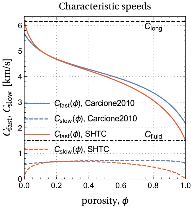
Figure 1: Comparison of the characteristic speeds for the Biot and SHTC models for the material parameters given in Table 1. Biot's model is taken in the version developed by Carcione et al [6].

In Fig 1, for the two models, we compare the characteristic speeds $C_{\textrm{f}ast}(\phi)$ and $C_{\textrm{s}low}(\phi)$ of the fast and slow modes. Some other material parameters are given in Table 1. Note that, in order to make the curves closer to each other, the bulk moduli of the solid phase in the two models are taken slightly different.

In the limit cases $\phi\to 0$ (pure solid) and $\phi\to 1$ (pure fluid) the behavior of the characteristic speeds in the SHTC model better corresponds to that intuitively expected, i.e. the characteristic speeds of the mixture coincide with the characteristic speeds of the pure phases (horizontal dashed and dashed-dotted lines), while the slow mode vanishes. In contrast, in Biot's model the slow mode is present even in the pure fluid or pure solid cases.

Parameters	Biot	SHTC	Unit
Grain:
$\rho_{\textrm{s}}=\rho_{2}$	2500	2500	kg/m3
$C_{\textrm{s}}$	4000	4332	m/s
$C_{\textrm{s}h}$	-	3787	m/s
$K_{\textrm{s}}=K_{2}=\rho_{2}C_{\textrm{s}}^{2}$	40	46.9	GPa
$\mu_{\textrm{s}}=\mu=\rho_{2}C_{\textrm{s}h}^{2}$	-	35.85	GPa
Matrix, $\phi=0.2$:
$K_{\textrm{m}}$	$9.48$	-	GPa
$\mu_{\textrm{m}}$	$24.5$	-	GPa
${\mathcal{T}}$	$3.75$	-	-
$\kappa$	$1\cdot 10^{-13}$	-	m2
$\theta_{2}$	-	$3.36\cdot 10^{-7}$	s
Fluid:
$\rho_{\textrm{f}}=\rho_{1}$	1040	1040	kg/m3
$C_{\textrm{f}}$	1500	1500	m/s
$K_{\textrm{f}}=K_{1}=\rho_{\textrm{f}}C_{\textrm{f}}^{2}$	2.34	2.34	GPa
$\eta$	$10^{-3}$	-	Pa$\cdot$ s

Table 1: Material parameters for the Biot and SHTC models. Here $C_{\textrm{s}}$ and $C_{\textrm{f}}$ are the bulk sound speeds in the solid and fluid, respectively.

4.2.3 Dispersion relations and sound speeds

In this section, we will perform a plane wave analysis of the SHTC and Biot models. Moreover, we will consider only longitudinal waves. In this case the vector of SHTC state variables reduces to

$${\bm{Q}}=(v_{1},w_{1},p,s_{11}).$$ (71)

By linearizing the right hand-side of system (45) in a neighborhood of ${\bm{Q}}={\bm{Q}}_{0}+{\bm{q}}$, where ${\bm{q}}$ is a small perturbation of an equilibrium state ${\bm{Q}}_{0}=(0,0,p_{0},0)$, we have

$${\bm{q}}_{t}+\mathbb{A}{\bm{q}}_{x}=\mathbb{S}{\bm{q}},$$ (72)

where $\mathbb{A}$ and $\mathbb{S}=\partial\SS/\partial{\bm{Q}}$ are matrices taken at the equilibrium state ${\bm{Q}}_{0}$:

$$\mathbb{A}=\left(\begin{array}[]{cccc}0&0&\rho^{-1}&\alpha_{2}\rho^{-1}\\ 0&0&R&0\\ K&K^{\prime}&0&0\\ -\frac{4}{3}\mu&0&0&0\end{array}\right),$$ (77)

$$\mathbb{S}=\left(\begin{array}[]{cccc}0&0&0&0\\ 0&-\frac{1}{\theta_{2}^{\prime}}&0&0\\ 0&0&0&0\\ 0&0&0&0\end{array}\right).$$ (82)

We seek a solution that has the form

$${\bm{q}}=\tilde{{\bm{q}}}e^{\text{i}(\omega t-kx)},$$ (83)

which represents a plane harmonic wave of real frequency $\omega$ and complex wave number $k$ propagating in the direction $x$, and $\tilde{{\bm{q}}}=const$ is a constant vector of amplitudes. By substituting (83) in (72), we arrive at a homogeneous linear system for $\tilde{{\bm{q}}}$ [24, 41]:

$$\left(\mathbb{I}-\frac{k}{\omega}\mathbb{A}+\frac{\text{i}}{\omega}\mathbb{S}\right)\tilde{{\bm{q}}}=0$$ (84)

where $\mathbb{I}$ is the identity matrix of the same size as $\mathbb{A}$ and $\mathbb{S}$. From (84) we have the following dispersion relation for (45):

$$\det\left(\mathbb{I}-\frac{k}{\omega}\mathbb{A}+\frac{\text{i}}{\omega}\mathbb{S}\right)=0.$$ (85)

The phase velocity $V_{\textrm{p}h}$ (sound speed) and the attenuation factor $a$ are then given by

$$V_{\textrm{p}h}=\frac{\omega}{{\textrm{R}e}(k)},\qquad a=-{\textrm{I}m}(k).$$ (86)

In addition, it is convenient to use the attenuation per wavelength [41]

$$a_{\lambda}=a\lambda=\frac{2\pi V_{\textrm{p}h}a}{\omega}=-2\pi\frac{{\textrm{I}m}(k)}{{\textrm{R}e}(k)},$$ (87)

where $\lambda$ is the wavelength.

There are four solutions to (85) with matrices (77), which are

$${\scriptstyle k(\omega)=\pm\omega\sqrt{\frac{X+Y-{\textrm{i}}(Y+Z)/\Omega\pm\sqrt{4Y(X-Z)({\textrm{i}}/\Omega-1)+({\textrm{i}}(Y+Z)/\Omega-(X+Y))^{2}}}{2(X-Z)Y}},}$$ (88)

where $X,Y$, and $Z$ are defined in (68), and $\Omega=\omega\theta_{2}^{\prime}$ is the non-dimensional frequency.

Applying the same analysis to the Biot equations (43), we find that the dispersion relation is a bi-quadratic equation

$$\lambda^{4}+a_{2}\lambda^{2}+a_{0}=0,$$ (89a)

$$a_{2}=\omega\left(-\frac{\omega({\mathcal{T}}\rho_{\textrm{f}}(\lambda_{\textrm{u}}+2\mu_{\textrm{u}})+M\phi(\rho-2\alpha\rho_{\textrm{f}}))}{\phi M\left(\lambda_{\textrm{u}}+2\mu_{\textrm{u}}-\alpha^{2}M\right)}\right.$$

$$\left.+\frac{{\textrm{i}}\eta(\lambda_{\textrm{u}}+2\mu_{\textrm{u}})}{\kappa M\left(\lambda_{\textrm{u}}+2\mu_{\textrm{u}}-\alpha^{2}M\right)}\right),$$ (89b)

$$a_{0}=\omega^{3}\left(\frac{\rho_{\textrm{f}}\omega({\mathcal{T}}\rho-\rho_{\textrm{f}}\phi)}{\phi M\left(\lambda_{\textrm{u}}+2\mu_{\textrm{u}}-\alpha^{2}M\right)}-\frac{{\textrm{i}}\eta\rho}{\kappa M\left(\lambda_{\textrm{u}}+2\mu_{\textrm{u}}-\alpha^{2}M\right)}\right).$$ (89c)

The phase velocities $V_{\textrm{p}h}(\omega)$ and attenuation factor per wavelength $a_{\lambda}(\omega)$ of the fast and slow sound waves for both models are shown in Fig. 2. Note that there is a difference in the high-frequency limit of the fast modes, which is, in fact, due to the difference between the characteristic speeds $C_{\textrm{f}ast}$ and $C_{\textrm{s}low}$ depicted in Fig. 1. To explain this, recall that the characteristic speeds (the eigenvalues of the homogeneous hyperbolic system) are the high-frequency limits ($\omega\to\infty$) of the sound speeds (the eigenvalues of the non-homogeneous system (72)) [24, 41, 9]. The slow mode dispersion curves of both models are almost indistinguishable, see Fig. 2, the second column.

Another conclusion is that there is a big difference ($\sim 10^{3}$) in the attenuation factors $a_{\lambda}$ of the fast and slow modes for both models in the low frequency region, see Fig. 2, the second row.

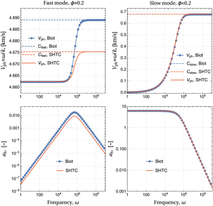
Figure 2: Phase velocities (first row) and attenuation factors per wavelength (second row) for the fast (first column) and slow (second column) modes of the SHTC and Biot models. The material parameters are given in Table 1.

5 Numerical test problems for small-amplitude wave propagation

5.1 Finite difference implementation

To discretize the governing equations, the velocity-stress formulation, which was proposed for elastic-wave equations in [20, 43], is used. The use of a numerical scheme on staggered grids is quite natural due to the fact that the equations form a symmetric first order system of evolution equations for the mixture components, relative velocities, pressure, and shear stress.

Following the notation of [43] and [16], we introduce a time-space grid with integer nodes $t^{n}=n\Delta t$, $x_{i}=i\Delta x$, $y_{j}=j\Delta y$ and half-integer nodes $t^{n+1/2}=(n+1/2)\Delta t$, $x_{i+1/2}=(i+1/2)\Delta x$, $y_{j+1/2}=(j+1/2)\Delta y$ , where $\Delta t$, $\Delta x$, and $\Delta y$ denote the grid step sizes for the temporal and spatial axes.

For a discrete function $f_{i,j}^{n}=f(t^{n},x_{i},y_{j})$ defined at the grid nodes, let us introduce second-order centered finite difference operators:

$$D_{t}[f]_{i,j}^{n}=\frac{(f)_{i,j}^{n+1/2}-(f)_{i,j}^{n-1/2}}{\Delta t},$$

$$A_{t}[f]_{i,j}^{n}=\frac{(f)_{i,j}^{n+1/2}+(f)_{i,j}^{n-1/2}}{2},$$ (90)

$$D_{x}[f]_{i,j}^{n}=\frac{(f)_{i+1/2,j}^{n}-(f)_{i-1/2,j}^{n}}{\Delta x},$$

$$D_{y}[f]_{i,j}^{n}=\frac{(f)_{i,j+1/2}^{n}-(f)_{i,j-1/2}^{n}}{\Delta y}.$$ (91)

The medium parameters are constant within each grid cell $[x_{i-1/2},x_{i+1/2}]\times[y_{j-1/2},y_{j+1/2}]$, and they may have discontinuities aligned with grid lines. This condition provides second-order convergence even for discontinuous medium parameters [23].

The wavefield components are defined at different time-space grid nodes. The components of the mixture and the relative velocities are defined as $(v_{x})_{i+1/2,j}^{n}$, $(v_{y})_{i,j+1/2}^{n}$, $(w_{x})_{i+1/2,j}^{n}$, $(w_{y})_{i,j+1/2}^{n}$, the pressure and the normal components of the deviatoric stress as $(p)_{i,j}^{n+1/2}$, $(s_{xx})_{i,j}^{n+1/2}$, $(s_{yy})_{i,j}^{n+1/2}$, and the shear stress as $(s_{xy})_{i+1/2,j+1/2}^{n+1/2}$.

To construct the finite difference scheme, we use a finite volume approximation or balance law technique [42]. In this case the discrete form of equations (38) reads as

$$D_{t}[v_{x}]_{i+1/2,j}^{n-1/2}=-\left\langle 1/\rho^{0}\right\rangle_{i+1/2,j}D_{x}[P]_{i+1/2,j}^{n-1/2}$$

$$+\left\langle\alpha_{2}^{0}/\rho^{0}\right\rangle_{i+1/2,j}\left(D_{x}[s_{xx}]_{i+1/2,j}^{n-1/2}+D_{y}[s_{xy}]_{i+1/2,j}^{n-1/2}\right),$$ (92a)

$$D_{t}[v_{y}]_{i,j+1/2}^{n-1/2}=-\left\langle 1/\rho^{0}\right\rangle_{i,j+1/2}D_{y}[P]_{i,j+1/2}^{n-1/2}$$

$$+\left\langle\alpha_{2}^{0}/\rho^{0}\right\rangle_{i,j+1/2}\left(D_{x}[s_{xy}]_{i,j+1/2}^{n-1/2}+D_{y}[s_{yy}]_{i,j+1/2}^{n-1/2}\right),$$ (92b)

$$D_{t}[w_{x}]_{i+1/2,j}^{n-1/2}=-\left\langle 1/\rho_{1}^{0}-1/\rho_{2}^{0}\right\rangle_{i+1/2,j}D_{x}[P]_{i+1/2,j}^{n-1/2}$$

$$-\left\langle c_{1}^{0}c_{2}^{0}/\theta_{2}\right\rangle_{i+1/2,j}A_{t}[w_{x}]_{i+1/2,j}^{n-1/2},$$ (92c)

$$D_{t}[w_{y}]_{i,j+1/2}^{n-1/2}=-\left\langle 1/\rho_{1}^{0}-1/\rho_{2}^{0}\right\rangle_{i,j+1/2}D_{y}[P]_{i,j+1/2}^{n-1/2}$$

$$-\left\langle c_{1}^{0}c_{2}^{0}/\theta_{2}\right\rangle_{i,j+1/2}A_{t}[w_{y}]_{i,j+1/2}^{n-1/2},$$ (92d)

$$D_{t}[s_{xx}]_{i,j}^{n}=(\mu)_{i,j}\left(\frac{4}{3}D_{x}[v_{x}]_{i,j}^{n}-\frac{2}{3}D_{y}[v_{y}]_{i,j}^{n}\right)$$

$$-(\alpha_{2}^{0}/\tau)_{i,j}A_{t}[s_{xx}]_{i,j}^{n},$$ (92e)

$$D_{t}[s_{yy}]_{i,j}^{n}=(\mu)_{i,j}\left(\frac{4}{3}D_{y}[v_{y}]_{i,j}^{n}-\frac{2}{3}D_{x}[v_{x}]_{i,j}^{n}\right)$$

$$-(\alpha_{2}^{0}/\tau)_{i,j}A_{t}[s_{yy}]_{i,j}^{n},$$ (92f)

$$\begin{array}[]{c}D_{t}[s_{xy}]_{i+1/2,j+1/2}^{n}=\left\{\mu\right\}_{i+1/2,j+1/2}\left(D_{x}[v_{y}]_{i+1/2,j+1/2}^{n}\right.\\ \left.+D_{y}[v_{x}]_{i+1/2,j+1/2}^{n}\right)-\left\{\alpha_{2}^{0}/\tau\right\}_{i+1/2,j+1/2}A_{t}[s_{xy}]_{i+1/2,j+1/2}^{n},\end{array}$$ (92g)

$$D_{t}[P]_{i,j}^{n}=-(K)_{i,j}\left(D_{x}[v_{x}]_{i,j}^{n}+D_{y}[v_{y}]_{i,j}^{n}\right)-$$

$$-\left((\rho_{2}^{0}-\rho_{1}^{0})\alpha_{1}^{0}\alpha_{2}^{0}K/\rho^{0}\right)_{i,j}\left(D_{x}[w_{x}]_{i,j}^{n}+D_{y}[w_{y}]_{i,j}^{n}\right),$$ (92h)

where the effective medium parameters on the staggered grids are obtained as volume arithmetic or harmonic averaging [23]:

$$\left\langle f\right\rangle_{i+1/2,j}=(f_{i,j}+f_{i+1,j})/2,$$

$$\left\langle f\right\rangle_{i,j+1/2}=(f_{i,j}+f_{i,j+1})/2,$$

$$\left\{f\right\}_{i+1/2,j+1/2}=4/\left(\dfrac{1}{f_{i,j}}+\dfrac{1}{f_{i+1,j}}+\dfrac{1}{f_{i,j+1}}+\dfrac{1}{f_{i+1,j+1}}\right).$$ (93)

The thus obtained 2D velocity-stress finite difference scheme is second-order accurate in both time and space. Note that the approximation can be easily improved by using higher order operators. The well-known Courant-Friedrichs-Lewy (CFL) stability criterion also holds for this case: the time step must be chosen small enough in order that the fastest characteristic wave (P-wave) $C_{max}$ travel a distance smaller than the spatial discretization step:

$$\Delta tC_{max}\sqrt{\frac{1}{{\Delta x}^{2}}+\frac{1}{{\Delta y}^{2}}}\leq 1.$$

A forcing function $f(t,x,y)$ is introduced as the source term in the right-hand side of the pressure equation or the equations for the normal components of the deviatoric stress in system (38). In both cases, a volumetric-type source term is obtained. The source function is defined as the product of Dirac's delta function in space and Ricker's wavelet in time:

$$f(t)=(1-2\pi^{2}f_{0}^{2}(t-t_{0})^{2})exp[-\pi^{2}f_{0}^{2}(t-t_{0})^{2}],$$ (94)

where $f_{0}$ is the source peak frequency and $t_{0}$ is the wavelet delay.

No special care is taken to suppress the outgoing waves with the help of absorbing boundary conditions (for example, PML). The simulation is stopped before the waves have reached the boundaries of the computational domain. The numerical experiments have been performed on a desktop computer with Intel(R) Core(TM) i7 3.60 GHz processor.

In the subsequent sections, we will illustrate the main features of wavefield formation and propagation depending on porosity $\phi$, friction parameter $\theta_{2}$, source peak frequency $f_{0}$, and shear relaxation time $\tau$. Before doing this, we start with considering the homogeneous dissipation-less case.

5.2 Dependence on porosity $\phi$.

The computational domain $\Omega=[-0.65,0.65]^{2}$ m was discretized with $N_{x}\times N_{y}$ grid points, $N_{x}=N_{y}=3250$, which amounts to 10 points per slow compressional wavelength in $\Omega$ for a source of central frequency $f_{0}=10^{5}$ Hz and for various values of porosity $\phi$. The model parameters were taken from Table 1. The source was located in the center of the computational domain. The propagation time was chosen to be equal to $T_{0}=1.1\cdot 10^{-4}$ s with source time delay $t_{0}=1/f_{0}$=$0.1\cdot 10^{-4}$ s. The time step was chosen according to the classical Courant stability criterion for staggered grids with $CFL=0.9$.

Fig. 3(a) shows a snapshot of the mixture velocity $v^{1}$ at time $T_{0}$, on the whole computational domain. The porosity parameter was chosen to be equal to $\phi$=0, which corresponds to the case of a pure elastic solid. In an elastic medium, only one fast P-wave with a velocity equal to 6155 m/s is excited from a source of volumetric type. The seismogram in Fig.  3(b) confirms the occurrence of this wave with the predicted velocity. The receivers were located along the $x$-axis starting from the source point towards the boundary with a uniform spacing between the receivers.

(a)

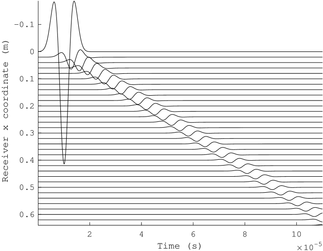
(b)

Figure 3: Wavefield in the pure elastic medium generated by the Ricker wavelet of a volumetric type. A snapshot at time $T_{0}=1.1\cdot 10^{-4}$ s (a) and seismogram (b) of the horizontal mixture velocity $v^{1}$ for source of central frequency $f_{0}=10^{5}$ Hz.

Fig. 4 shows the results of calculations similar to the previous ones but with porosity parameter $\phi$=1. This corresponds to the case of a pure liquid with one pressure wave with a velocity of 1500 m/s. The numerical propagation velocity can be easily estimated from the computed seismogram in Fig. 4(b) to be exactly 1500 m/s.

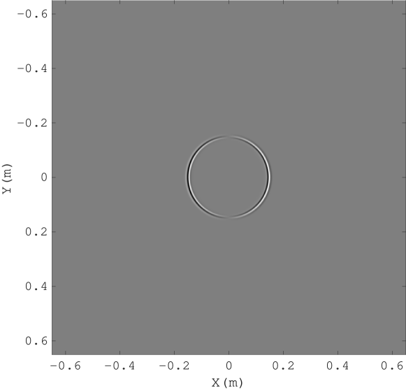
(a)

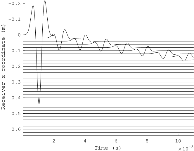
(b)

Figure 4: Wavefield in the pure fluid generated by the Ricker wavelet of a volumetric type. A snapshot at time $T_{0}=1.1\cdot 10^{-4}$ s (a) and seismogram (b) of the mixture horizontal velocity $v^{1}$ for source of central frequency $f_{0}=10^{5}$ Hz.

The simulation results for porosity parameter $\phi$=0.5 are shown in Fig. 5. The fast P-wave velocity is estimated to be 4100 m/s from the computed seismogram in Fig. 5(b), which is consistent with the data from Table 1. In the snapshot of Fig. 5(a) we do not observe the predicted slow P-wave because it is completely attenuated, not visible at this time, and its amplitude is very small. However, if we zoom in the image, we will be able to see this slow P-wave in Fig. 6.

(a)

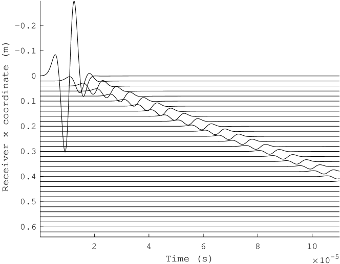
(b)

Figure 5: Wavefield in the porous medium with porosity $\phi=0.5$ generated by the Ricker wavelet of a volumetric type. A snapshot at time $T_{0}=1.1\cdot 10^{-4}$ s (a) and seismogram (b) of the mixture horizontal velocity $v^{1}$ for source of central frequency $f_{0}=10^{5}$ Hz.

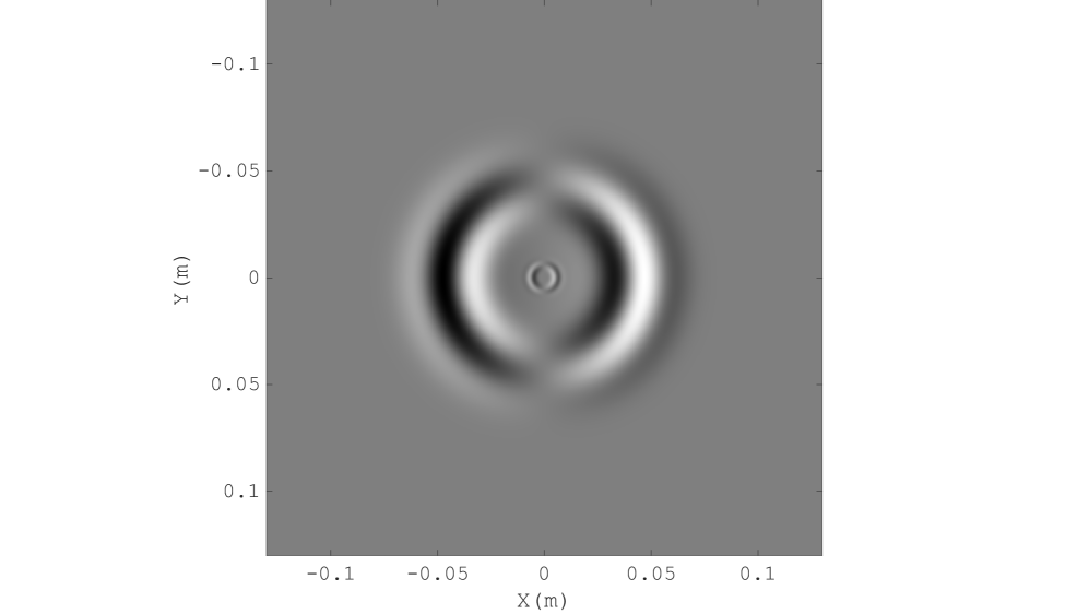
(a)

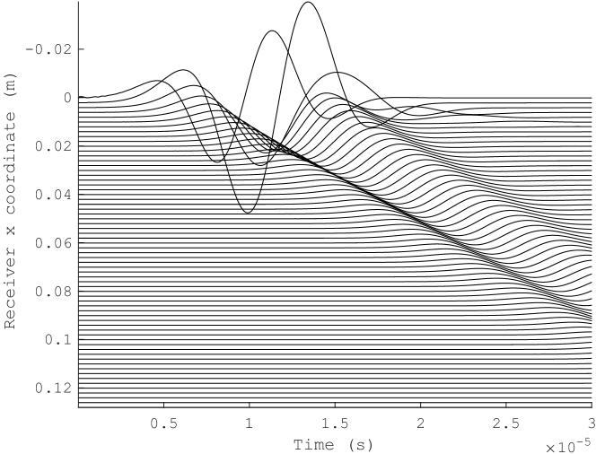
(b)

Figure 6: Wavefield in the porous medium with porosity $\phi=0.5$ generated by the Ricker wavelet of a volumetric type. A zoom of snapshot at time $1\cdot 10^{-5}$ s (a) and seismogram (b) of the mixture horizontal velocity $v^{1}$ for source of central frequency $f_{0}=10^{5}$ Hz.

The amplitude variation for several values of $\phi$ can also be seen in Fig. 7, where the wavefield distribution along the $x$-axis for $y=0$ is presented.

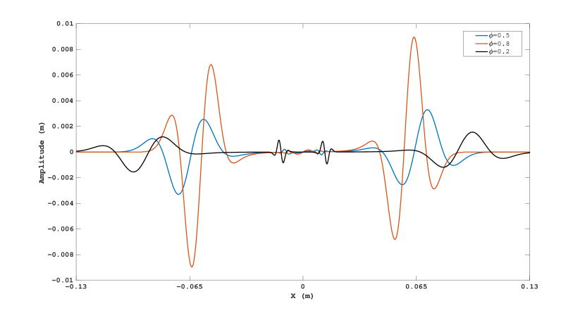
Figure 7: The distribution of the mixture horizontal velocity $v^{1}$ generated by the Ricker wavelet of a volumetric type along the $x$-axis at time $2.1\cdot 10^{-5}$ s and $y=0$ for several values of porosity $\phi$: $\phi=0.2$ (black), $\phi=0.5$ (blue), $\phi=0.8$ (red).

Summarizing the results of numerical experiments of this section, we conclude that by varying porosity $\phi$ in system (38), it is possible to correctly describe the three states of the medium: liquid, solid, and poroelastic.

5.3 Dependence on friction $\theta_{2}$.

In this section, we study the behavior and properties of the fast and slow P-waves, depending on the parameter $\theta_{2}$. This parameter is present as the denominator in the right-hand side of the second equation in system (38). By analogy with Biot's model, $\theta_{2}$ can be viewed as a friction parameter, because it controls interfacial friction in a multiphase medium and leads to wave dispersion and attenuation.

Consider the same homogeneous numerical model as in the previous sections with $\theta_{2}$ equal to $3.36\cdot 10^{-7}$ from Table 1. Let us observe the behavior of the P-waves if we increase or decrease this parameter twice. Fig. 8(a-c) shows snapshots of the mixture velocity $v^{1}$ for these three values of $\theta_{2}$. Significant wave amplitude variations are observed only for slow P-wave. More detailed variations of the amplitudes can be seen in Fig. 9, where the wavefield along the $x$-axis at $y=0$ is presented. This figure demonstrates an increase in the amplitude of the slow P-wave with increasing $\theta_{2}$, and vice versa. A change in the form of slow waves is also observed, while the fast wave remains almost unchanged.

Summarizing the results of numerical experiments of this section, we conclude that by varying the parameter $\theta_{2}$ in system (38) it is possible to affect the amplitude and propagation velocity of the slow P-wave. One of the interesting applications, in our opinion, can be the solution of the inverse problem of determining the coefficient $\theta_{2}$ by analyzing the ratio of the amplitudes of the fast and slow waves in a field experiment.

(a) $\quad\quad\theta_{2}=3.36\cdot 10^{-7}$

(b) $\quad\quad\theta_{2}=2\cdot 3.36\cdot 10^{-7}$

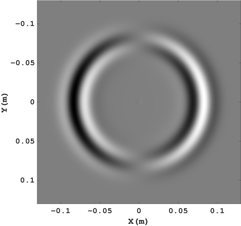
(c) $\quad\quad\theta_{2}=1/2\cdot 3.36\cdot 10^{-7}$

Figure 8: Wavefield in the porous medium with porosity $\phi=0.5$ generated by the Ricker wavelet of a volumetric type. Snapshots at time $2.1\cdot 10^{-5}$ s of the horizontal mixture velocity $v^{1}$ for several values of $\theta_{2}$.

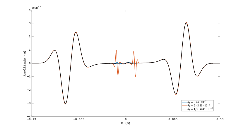
Figure 9: A comparison at time $2.1\cdot 10^{-5}$ s of values of the mixture velocity $v^{1}$ for several values of $\theta_{2}$: $\theta_{2}=3.36\cdot 10^{-7}$ (blue), $\theta_{2}=2\cdot 3.36\cdot 10^{-7}$ (red), $\theta_{2}=1/2\cdot 3.36\cdot 10^{-7}$ (black).

5.4 Dependence on frequency $f_{0}$.

In this section, we perform a study of dispersion of the wave velocity depending on the source peak frequency $f_{0}$ based on the same homogeneous numerical model with parameters from Table 1 as in the previous sections. The dispersion curves in Fig. 1 show that the main velocity changes are in the range of $10^{4}-10^{6}$ Hz. Because of a difference of three orders of magnitude in the frequency range, our comparison will be made not for a single computational domain, but for three different domains. More specifically, we use a ten orders of magnitude scaling of both space and time. Fig. 10 presents snapshots, and Fig. 11 presents seismograms of the mixture velocity $v^{1}$ for several frequencies. For each time frequency, a snapshot is recorded at time $5/{f_{0}}$ (including a shift wavelet delay of $1/{f_{0}}$) for square domains with a side of $5$ m (for $f_{0}=10^{4}$), $0.5$ m (for $f_{0}=10^{5}$), and $0.05$ m (for $f_{0}=10^{6}$). The time and size are chosen in such a way that in the isotropic elastic case we can obtain three identical snapshots. As expected in the poroelastic case, we observe wavefield differences which are most clearly seen in the seismograms: the lower the frequency, the stronger the dispersion and attenuation of the slow P-wave. To estimate the phase velocity, we use a spectral ratio technique [17], [7] and obtain a phase velocity $v_{p}=420$ m/s for a frequency $f_{0}=10^{5}$ Hz and $v_{p}=670$ m/s for the frequency $f_{0}=10^{6}$ Hz. It is not possible to make similar estimation for a frequency $f_{0}=10^{4}$ due to the fact that the slow wave has a low amplitude. We can also conclude that the attenuation of the slow P-wave is sufficiently strong even for high frequencies.

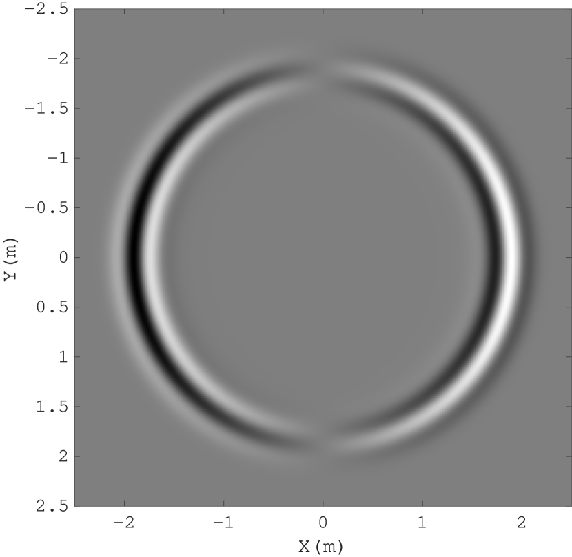
(a) $\quad\quad f_{0}=10^{4}$

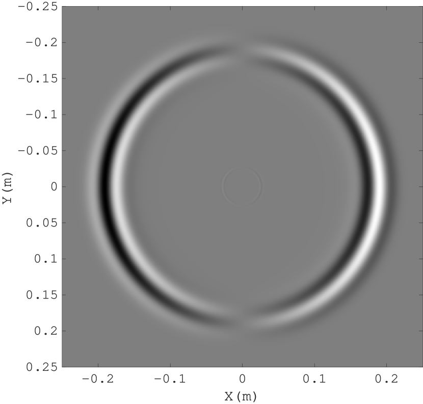
(b) $\quad\quad f_{0}=10^{5}$

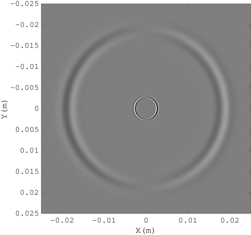
(c) $\quad\quad f_{0}=10^{6}$

Figure 10: Wavefield in the porous medium with porosity $\phi=0.5$ generated by the Ricker wavelet of a volumetric type. Snapshots of the horizontal mixture velocity $v^{1}$ for several frequencies: $f_{0}=10^{4}$ Hz (a), $f_{0}=10^{5}$ Hz (b), $f_{0}=10^{6}$ Hz (c).

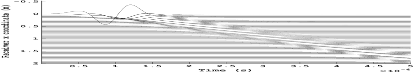
(a) $\quad\quad f_{0}=10^{4}$

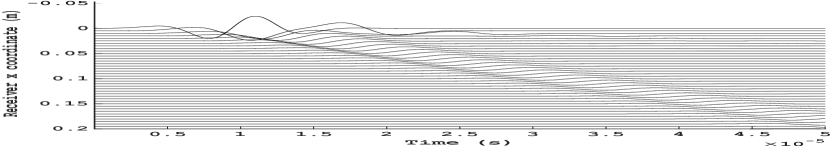
(b) $\quad\quad f_{0}=10^{5}$

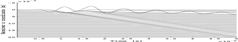
(c) $\quad\quad f_{0}=10^{6}$

Figure 11: Wavefield in the porous medium with porosity $\phi=0.5$ generated by the Ricker wavelet of a volumetric type. Seismograms of the horizontal mixture velocity $v^{1}$ for several frequencies: $f_{0}=10^{4}$ Hz (a), $f_{0}=10^{5}$ Hz (b), $f_{0}=10^{6}$ Hz(c).

5.5 Dependence on shear relaxation time.

The aim of this section is to show that there is an additional mechanism of energy dissipation embedded in system (38) and controlled by the relaxation parameter $\tau$ in the right-hand side of equation (38d). A proper choice of the relaxation time $\tau$ allows one to model irreversible (elastoplastic) deformations in the solid matrix, e.g. [8, 33], or viscous flows [9].

All the previous numerical examples were simulated without relaxation of tangential shear stresses, that is, the right-hand side in (38d) vanished. Formally, this corresponds to the case of $\tau=\infty$. It is quite obvious that, for finite values of $\tau$, the mechanism of relaxation of tangential stresses provides an additional ability of the model to control wave attenuation. To this end, we again consider the example from the previous Section 5.4 for a frequency $f_{0}=10^{4}$ Hz and compare the solution with a similar test, but with allowance for relaxation of tangential stresses.

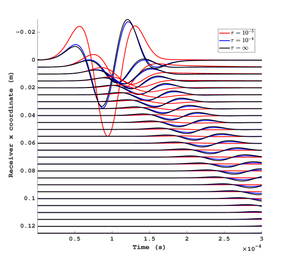
Figure 12: Comparison of seismograms of the horizontal mixture velocity $v^{1}$ for several values of shear relaxation time $\tau$: no relaxation (black), $\tau=10^{-5}$ (red), $\tau=10^{-4}$ (blue).

As expected, a comparison of the seismograms in Fig. 12 shows that relaxation of tangential stresses leads to dispersion and attenuation of seismic waves. On the distant receivers, it is seen that the smaller $\tau$, the greater the attenuation. On the nearer receivers, dispersion probably has a predominant effect.

5.6 Layered media.

This test illustrates the effects of the interfaces between pure fluid, poroelastic and pure elastic media on an example of a three-layered medium with the media parameters from Table 1. The size of the computational domain is $0.025$ m in the $x$ and $y$ directions. The upper layer is water, the lower layer is an elastic medium and in the middle, from $-0.005$ m to $0.005$ m, there is a poroelastic layer with porosity $\phi$=0.2. A source of central frequency $f_{0}=10^{6}$ Hz is located in the water layer at the point $x=0,y=-0.01$.

In order to present all types of waves, let us consider snapshots of the total velocity vector for different moments of time. We strongly amplified the wavefield amplitude in Fig. 13 to be able to pick out the slow compressional waves in the snapshots. In order to interpret the waves arising in the medium, we use 'P' to mark P-waves and 'S' to mark S-waves. The subscript 'r' indicates the reflected waves, while the subscript 't' indicates the transmitted waves. Also, we use the subscript 's' to identify a slow P-wave and the subscript 'f' to identify a pressure wave in the fluid layer.

The source in the water layer excites a pressure wave ( denoted by P${}_{\textrm{f}}$ in Fig. 13) which propagates towards the poroelastic layer. This wave then reflects from the bottom of the water-poroelastic interface (P${}_{\textrm{f}}$P${}_{\textrm{r}}$) and generates a fast transmitted P-wave (P${}_{\textrm{f}}$P${}_{\textrm{t}}$), a slow transmitted P-wave (P${}_{\textrm{f}}$P${}_{\textrm{s}}$), and a transmitted S-wave (P${}_{\textrm{f}}$S${}_{\textrm{t}}$) in the poroelastic medium. Afterwards, these waves generate a family of transmitted and reflected waves (including a transmitted P-wave (P${}_{\textrm{f}}$P${}_{\textrm{t}}$P${}_{\textrm{t}}$), an S-wave (P${}_{\textrm{f}}$S${}_{\textrm{t}}$S${}_{\textrm{t}}$), and a reflected slow P-wave (P${}_{\textrm{f}}$P${}_{\textrm{t}}$P${}_{\textrm{s}}$)) from the upper and lower boundaries of the poroelastic layer.

In this example we see that the propagation of all types of waves predicted by the elasticity and poroelasticity theories is correct: slow waves arise only in the poroelastic layer, only pressure waves propagate in the liquid layer, while longitudinal and shear waves appear in the elastic medium.

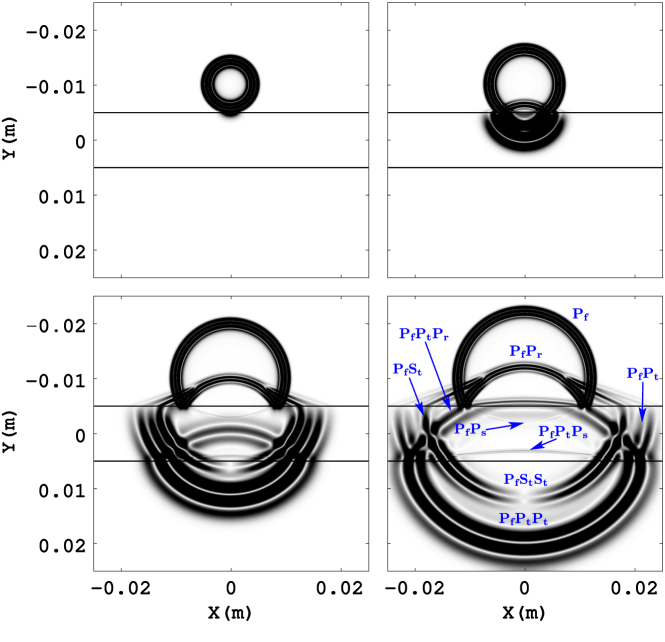
Figure 13: Snapshots of the norm of mixture velocity $||v||^{2}$ for a layered medium: water (upper layer, $\phi=1$), poroelastic (middle layer, $\phi=0.2$) and elastic solid (bottom layer, $\phi=0$).

6 Conclusions

An extension of the unified model of continuum fluid and solid mechanics [9] for compressible fluid flows in elastoplastic porous media has been proposed. The derivation is based on the Symmetric Hyperbolic Thermodynamically Compatible (SHTC) theory [32], and the resulting model represents a combination of the unified continuum model from [9] with the SHTC model for two-phase compressible flows from [36]. The governing equations satisfy two laws of thermodynamics (energy conservation and non-decreasing of entropy) and form a first-order symmetric system which is hyperbolic in the sense of Friedrichs [11] if the generating thermodynamic potential is convex.

Based on the above-proposed non-linear model, a linearized first order PDE system for small-amplitude wave propagation in a stationary saturated porous medium has been derived. The linear system is written in terms of the velocity of the solid-fluid mixture, and the relative velocity of the phase motion, pressure and shear stress. Such a formulation allowed us a straightforward development of an efficient finite difference scheme on a staggered grid.

A comparison of the above-proposed SHTC model and the classical Biot model for wave propagation in a saturated elastic porous medium has been made at the aid of the dispersion analysis. It turns out that, although the basic equations of the two models are different, the SHTC model is able to describe all the effects (in particular, the existence of a slow P-wave) predicted by Biot's theory, in good quantitative and qualitative agreement.

A number of two-dimensional test problems has been solved for the propagation of small-amplitude waves described by the formulated model. These test problems include, in particular, the study of the dependence of wavefields on model parameters. The numerical results demonstrate that the SHTC model describes correctly all physical characteristics of the process.

Finally, we note that the developed poroelastic model is based on the SHTC formulation of mixtures. It thus should be kept in mind that other approaches to obtain continuum models for mixtures are possible [4, 26, 27]. In particular, on the PDE level, the continuum formulation for mixtures obtained in the GENERIC (General Equation for Non-Equilibrium Reversible-Irreversible Coupling) framework [26, 28] differs from the SHTC formulation for mixtures used in this paper by a term $\sim E_{w^{l}}\left(\frac{\partial w^{k}}{\partial x_{l}}-\frac{\partial w^{l}}{\partial x_{k}}\right)$ missing in equation (14e). Also, on the physical level, the GENERIC formulation may differ by a different interpretation of the state variables, e.g. see a discussion on the SHTC compatible and alternative Poisson brackets for heat conduction and the total momentum definition in [32]. Nevertheless, for the case of small amplitude waves, such differences should not result in a different linear system and, in particular, the extra term mentioned above should vanish similar to the term $v^{l}\left(\frac{\partial w^{k}}{\partial x_{l}}-\frac{\partial w^{l}}{\partial x_{k}}\right)$, see equation (38b). Perhaps, differences in solutions should appear in case of finite deformations of poroelastic continuum. We hope to investigate this in detail in future publications.

In memoriam

This paper is dedicated to the memory of Dr. Douglas Nelson Woods (^∗January 11^th 1985 - $\dagger$September 11^th 2019), promising young scientist and post-doctoral research fellow at Los Alamos National Laboratory. Our thoughts and wishes go to his wife Jessica, to his parents Susan and Tom, to his sister Rebecca and to his brother Chris, whom he left behind.

References

- [1] M.A. Biot ``Theory of propagation of elastic waves in a fluid-saturated porous solid. II. Higher frequency range'' In Journal of the Acoustical Society of America 28.2, 1956, pp. 179–191
- [2] M.A. Biot ``Theory of propagation of elastic waves in fluid-saturated porous solid. I. Low-frequency range'' In Journal of the Acoustical Society of America 28.2, 1956, pp. 168–178
- [3] M.A. Biot ``Mechanics of deformation and acoustic propagation in porous media:'' In Journal of Applied Physics 33.4, 1962, pp. 1482–1498
- [4] A M Blokhin and V N Dorovsky ``Mathematical Modelling in the Theory of Multivelocity Continuum'' Nova Science Publishers Inc., New York, 1995, pp. 183 URL: https://www.brownsbfs.co.uk/Product/Blokhin-A-M/Mathematical-Modelling-in-the-Theory-of-Multivelocity-Continuum/9781560722403
- [5] Saray Busto, Simone Chiocchetti, Michael Dumbser, Elena Gaburro and Ilya Peshkov ``High Order ADER Schemes for Continuum Mechanics'' In Frontiers in Physics 8, 2020 DOI: 10.3389/fphy.2020.00032
- [6] José M. Carcione, Christina Morency and Juan E. Santos ``Computational poroelasticity — A review'' In Geophysics 75.5, 2010, pp. 75A229–75A243 DOI: 10.1190/1.3474602
- [7] Eva Caspari, Mikhail Novikov, Vadim Lisitsa, Nicolás D. Barbosa, Beatriz Quintal, J. Germán Rubino and Klaus Holliger ``Attenuation mechanisms in fractured fluid-saturated porous rocks: a numerical modelling study'' In Geophysical Prospecting 67.4, 2019, pp. 935–955 DOI: 10.1111/1365-2478.12667
- [8] Michael Dumbser, Ilya Peshkov and Evgeniy Romenski ``A Unified Hyperbolic Formulation for Viscous Fluids and Elastoplastic Solids'' In Theory, Numerics and Applications of Hyperbolic Problems II. HYP 2016 237, Springer Proceedings in Mathematics and Statistics Cham: Springer International Publishing, 2018, pp. 451–463 DOI: 10.1007/978-3-319-91548-7_34
- [9] Michael Dumbser, Ilya Peshkov, Evgeniy Romenski and Olindo Zanotti ``High order ADER schemes for a unified first order hyperbolic formulation of continuum mechanics: Viscous heat-conducting fluids and elastic solids'' In Journal of Computational Physics 314, 2016, pp. 824–862 DOI: 10.1016/j.jcp.2016.02.015
- [10] Michael Dumbser, Ilya Peshkov, Evgeniy Romenski and Olindo Zanotti ``High order ADER schemes for a unified first order hyperbolic formulation of Newtonian continuum mechanics coupled with electro-dynamics'' In Journal of Computational Physics 348 Elsevier Inc., 2017, pp. 298–342 DOI: 10.1016/j.jcp.2017.07.020
- [11] K O Friedrichs ``Symmetric positive linear differential equations'' In Communications on Pure and Applied Mathematics 11.3, 1958, pp. 333–418 DOI: 10.1002/cpa.3160110306
- [12] S K Godunov ``An interesting class of quasilinear systems'' In Dokl. Akad. Nauk SSSR 139(3), 1961, pp. 521–523
- [13] S. K. Godunov, T. Yu. Mikhaîlova and E. I. Romenskiî ``Systems of thermodynamically coordinated laws of conservation invariant under rotations'' In Siberian Mathematical Journal 37.4 Springer, 1996, pp. 690–705 DOI: 10.1007/BF02104662
- [14] S. K. Godunov and E. I. Romenski ``Thermodynamics, conservation laws, and symmetric forms of differential equations in mechanics of continuous media'' In Computational Fluid Dynamics Review 95 John Wiley, NY, 1995, pp. 19–31
- [15] S. K. Godunov and E. Romenskii ``Elements of Continuum Mechanics and Conservation Laws'' Springer US, 2003, pp. 258
- [16] Robert W. Graves ``Simulating seismic wave propagation in 3D elastic media using staggered-grid finite differences'' In Bulletin of the Seismological Society of America 86.4, 1996, pp. 1091–1106
- [17] Boris Gurevich and Roman Pevzner ``How frequency dependency of Q affects spectral ratio estimates'' In GEOPHYSICS 80.2, 2015, pp. A39–A44 DOI: 10.1190/geo2014-0418.1
- [18] Haran Jackson and Nikos Nikiforakis ``A numerical scheme for non-Newtonian fluids and plastic solids under the GPR model'' In Journal of Computational Physics 387 Elsevier Inc., 2019, pp. 410–429 DOI: 10.1016/j.jcp.2019.02.025
- [19] A.R. Khoei and T. Mohammadnejad ``Numerical modeling of multiphase fluid flow in deforming porous media: A comparison between two- and three-phase models for seismic analysis of earth and rockfill dams'' In Computers and Geotechnics 38.2 Elsevier, 2011, pp. 142–166 DOI: 10.1016/j.compgeo.2010.10.010
- [20] Alan R. Levander ``Fourth-order finite-difference P-SV seismograms'' In Geophysics 53.11, 1988, pp. 1425–1436 DOI: 10.1190/1.1442422
- [21] Y. J. Masson, S. R. Pride and K. T. Nihei ``Finite difference modeling of Biot's poroelastic equations at seismic frequencies'' In Journal of Geophysical Research: Solid Earth 111,.B10305, 2006 DOI: 10.1029/2006JB004366
- [22] Andi Merxhani ``An introduction to linear poroelasticity'', 2016, pp. 1–38 arXiv: http://arxiv.org/abs/1607.04274
- [23] P. Moczo, J. Kristek, V. Vavrycuk, R. J. Archuleta and L. Halada ``3D heterogeneous staggered-grid finite-difference modeling of seismic motion with volume harmonic and arithmetic averaging of elastic moduli and densities'' In Bull. Seism. Soc. Am. 92.8, 2002, pp. 3042–3066
- [24] A Muracchini, T Ruggeri and L Seccia ``Dispersion relation in the high frequency limit and non linear wave stability for hyperbolic dissipative systems'' In Wave Motion 15.2 Elsevier, 1992, pp. 143–158
- [25] S. Ndanou, N. Favrie and S. Gavrilyuk ``Criterion of Hyperbolicity in Hyperelasticity in the Case of the Stored Energy in Separable Form'' In Journal of Elasticity 115.1, 2014, pp. 1–25 DOI: 10.1007/s10659-013-9440-7
- [26] Michal Pavelka, Václav Klika and Miroslav Grmela ``Multiscale Thermo-Dynamics'' Berlin, Boston: De Gruyter, 2018 DOI: 10.1515/9783110350951
- [27] Michal Pavelka, František Maršík and Václav Klika ``Consistent theory of mixtures on different levels of description'' In International Journal of Engineering Science 78 Elsevier Ltd, 2014, pp. 192–217 DOI: 10.1016/j.ijengsci.2014.02.003
- [28] Michal Pavelka, Václav Klika, Oğul Esen and Miroslav Grmela ``A hierarchy of Poisson brackets in non-equilibrium thermodynamics'' In Physica D: Nonlinear Phenomena 335, 2016, pp. 54–69 DOI: 10.1016/j.physd.2016.06.011
- [29] Francesco Pesavento, Bernhard A. Schrefler and Giuseppe Sciumè ``Multiphase Flow in Deforming Porous Media: A Review'' In Archives of Computational Methods in Engineering 24.2 Springer Netherlands, 2017, pp. 423–448 DOI: 10.1007/s11831-016-9171-6
- [30] I. Peshkov, M. Grmela and E. Romenski ``Irreversible mechanics and thermodynamics of two-phase continua experiencing stress-induced solid-fluid transitions'' In Continuum Mechanics and Thermodynamics 27.6 Springer Berlin Heidelberg, 2015, pp. 905–940 DOI: 10.1007/s00161-014-0386-1
- [31] Ilya Peshkov and Evgeniy Romenski ``A hyperbolic model for viscous Newtonian flows'' In Continuum Mechanics and Thermodynamics 28.1-2, 2016, pp. 85–104 DOI: 10.1007/s00161-014-0401-6
- [32] Ilya Peshkov, Michal Pavelka, Evgeniy Romenski and Miroslav Grmela ``Continuum mechanics and thermodynamics in the Hamilton and the Godunov-type formulations'' In Continuum Mechanics and Thermodynamics 30.6, 2018, pp. 1343–1378 DOI: 10.1007/s00161-018-0621-2
- [33] Ilya Peshkov, Walter Boscheri, Raphaël Loubère, Evgeniy Romenski and Michael Dumbser ``Theoretical and numerical comparison of hyperelastic and hypoelastic formulations for Eulerian non-linear elastoplasticity'' In Journal of Computational Physics 387, 2019, pp. 481–521 DOI: 10.1016/j.jcp.2019.02.039
- [34] Eduard Rohan and Vladimír Lukeš ``Modeling large-deforming fluid-saturated porous media using an Eulerian incremental formulation'' In Advances in Engineering Software 113 Elsevier, 2017, pp. 84–95 DOI: 10.1016/j.advengsoft.2016.11.003
- [35] E. Romenski ``Conservative formulation for compressible fluid flow through elastic porous media'' In In: Vázquez-Cendón et al. (eds) Numerical Methods for Hyperbolic Equations. Taylor & Francis Group, London, 2013, pp. 193–200
- [36] E Romenski, D Drikakis and E Toro ``Conservative Models and Numerical Methods for Compressible Two-Phase Flow'' In Journal of Scientific Computing 42(1), 2010, pp. 68–95
- [37] E Romenski, A D Resnyansky and E F Toro ``Conservative hyperbolic model for compressible two-phase flow with different phase pressures and temperatures'' In Quarterly of applied mathematics 65(2).2, 2007, pp. 259–279
- [38] E.I. Romenski ``Hyperbolic systems of thermodynamically compatible conservation laws in continuum mechanics'' In Mathematical and computer modelling 28(10), 1998, pp. 115–130
- [39] Evgeniy Romenski, Alexander A. Belozerov and Ilya M. Peshkov ``Conservative formulation for compressible multiphase flows'' In Quarterly of Applied Mathematics 74.1, 2016, pp. 113–136 DOI: 10.1090/qam/1409
- [40] E.I. Romensky ``Thermodynamics and Hyperbolic Systems of Balance Laws in Continuum Mechanics'' In In: Toro E.F. (eds) Godunov Methods. Springer, Boston, MA, 2001, pp. 745–761
- [41] Tommaso Ruggeri and Masaru Sugiyama ``Rational Extended Thermodynamics beyond the Monatomic Gas'' In Rational Extended Thermodynamics beyond the Monatomic Gas Cham: Springer International Publishing, 2015, pp. 1–376 DOI: 10.1007/978-3-319-13341-6
- [42] A. A. Samarskii ``The Theory of Difference Schemes'' CRC Press, 2001, pp. 786
- [43] Jean Virieux ``P-SV wave propagation in heterogeneous media; velocity-stress finite-difference method'' In Geophysics 51.4, 1986, pp. 889–901 DOI: 10.1190/1.1442147
- [44] K. Wilmanski ``A few remarks on Biot's model and linear acoustics of poroelastic saturated materials'' In Soil Dynamics and Earthquake Engineering 26.6-7, 2006, pp. 509–536 DOI: 10.1016/j.soildyn.2006.01.006
- [45] Krzysztof Wilmanski ``A Thermodynamic Model of Compressible Porous Materials with the Balance Equation of Porosity'' In Transport in Porous Media 32.1 Kluwer Academic Publishers, 1998, pp. 21–47 DOI: 10.1023/A:1006563932061
- [46] Kenneth W. Winkler, Hsui-Lin Liu and David Linton Johnson ``Permeability and borehole Stoneley waves: Comparison between experiment and theory'' In GEOPHYSICS 54.1, 1989, pp. 66–75 DOI: 10.1190/1.1442578