Randomized mixed Hölder function approximation
in higher-dimensions

Abstract.

The purpose of this paper is to extend the result of arXiv:1810.00823 to mixed Hölder functions on $[0,1]^{d}$ for all $d\geq 1$. In particular, we prove that by sampling an $\alpha$-mixed Hölder function $f:[0,1]^{d}\rightarrow\mathbb{R}$ at $\sim\frac{1}{\varepsilon}\left(\log\frac{1}{\varepsilon}\right)^{d}$ independent uniformly random points from $[0,1]^{d}$, we can construct an approximation $\tilde{f}$ such that

$$\|f-\tilde{f}\|_{L^{2}}\lesssim\varepsilon^{\alpha}\left(\log\textstyle{\frac{1}{\varepsilon}}\right)^{d-1/2},$$

with high probability.

1. Introduction

1.1. Introduction

A function $f:[0,1]^{2}\rightarrow\mathbb{R}$ is $(c,\alpha)$-mixed Hölder if

$$|f(x^{\prime},y)-f(x,y)|\leq c|x^{\prime}-x|^{\alpha},\quad|f(x,y^{\prime})-f(x,y)|\leq c|y^{\prime}-y|^{\alpha},$$

and

$$|f(x^{\prime},y^{\prime})-f(x^{\prime},y)-f(x,y^{\prime})+f(x,y)|\leq c(|x^{\prime}-x||y^{\prime}-y|)^{\alpha},$$

for all $x,x^{\prime},y,y^{\prime}\in[0,1]$. This definition extends to higher dimensions as follows. Let $R=I_{1}\times\cdots\times I_{d}\subseteq[0,1]^{d}$ be the $r$-dimensional box formed by taking the Cartesian product of $r$ intervals $I_{i_{1}}=[a_{i_{1}},a_{i_{1}}+h_{i_{1}}),\ldots,I_{i_{r}}=[a_{i_{r}},a_{i_{r}}+h_{i_{r}})$ and $d-r$ singleton sets $I_{i_{r+1}}=\{a_{i_{r+1}}\},\ldots,I_{i_{d}}=\{a_{i_{d}}\}$, where $i_{1},\ldots,i_{d}$ is a permutation of $1,\ldots,d$. We define the discrete mixed difference $\delta_{R}f$ by

(1) $$\delta_{R}f=(\delta_{h_{i_{1}}}\cdots\delta_{h_{i_{r}}}f)(a_{1},\ldots,a_{d}),$$

where $\delta_{h_{j}}$ is the $j$-th variable discrete difference operator defined by

$$(\delta_{h_{j}}f)(x_{1},\ldots,x_{d})=f(x_{1},\ldots,x_{j-1},x_{j}+h_{j},x_{j+1},\ldots,x_{d})-f(x_{1},\ldots,x_{d}).$$

Definition 1.1.

We say a function $f:[0,1]^{d}\rightarrow\mathbb{R}$ is $(c,\alpha)$-mixed Hölder if

(2) $$|\delta_{R}f|\leq c|R|^{\alpha},$$

for all $r\leq d$ dimensional boxes $R$, where $|R|$ is the $r$-dimensional measure of $R$.

For example, if $f:[0,1]^{d}\rightarrow\mathbb{R}$ satisfies the mixed derivative condition $\left|\partial^{\beta}f\right|\leq c$ on $[0,1]^{d}$ for all multi-indices $\beta\in\{0,1\}^{d}$, where $\partial^{\beta}=\partial^{\beta_{1}}_{x_{1}}\cdots\partial^{\beta_{d}}_{x_{d}}$, then it follows from the mean value theorem that $f$ is $(c,1)$-mixed Hölder. Thus, the Hölder continuity condition is to the condition that $|\partial_{x_{j}}f|$ is bounded for all indices $j\in\{1,\ldots,d\}$ as the mixed Hölder condition is to the condition that $|\partial^{\beta}f|$ is bounded for all multi-indices $\beta\in\{0,1\}^{d}$.

1.2. Motivation

We say that a function $f:[0,1]^{d}\rightarrow\mathbb{R}$ is $(c,\alpha)$-Hölder continuous if

$$|f(x)-f(y)|\leq c\|x-y\|^{\alpha},$$

for all $x,y\in[0,1]^{d}$, where $\|\cdot\|$ denotes the Euclidean norm. If a function $f:[0,1]^{d}\rightarrow\mathbb{R}$ is only known to be $(c,\alpha)$-Hölder continuous, then $\sim(\frac{1}{\varepsilon})^{d}$ samples of the function are needed to construct an approximation $\tilde{f}$ such that

$$\|f-\tilde{f}\|_{L^{\infty}}\lesssim\varepsilon^{\alpha},$$

where the implicit constant only depends on the constant $c>0$. Moreover, sampling $\sim(\frac{1}{\varepsilon})^{d}$ function values is necessary to achieve this approximation error in $L^{p}$ for any fixed $p\geq 1$. The fact that the number of required samples $\sim(\frac{1}{\varepsilon})^{d}$ grows exponentially with the dimension $d$ for any fixed $\varepsilon>0$ is an example of the curse of dimensionality. Even in moderate dimensions, such sampling requirements may be intractable in practical situations.

The mixed Hölder condition strengthens the Hölder condition by requiring that the mixed difference of $f$ with respect to each box is controlled by the measure of the box; more precisely, it requires that

(3) $$|\delta_{R}f|\lesssim|R|^{\alpha},$$

for all $r\leq d$ dimensional boxes $R$. We will see below that this stronger geometric condition makes it possible to beat the curse of dimensionality.

We remark that while this paper focuses on real-valued mixed Hölder functions defined on $[0,1]^{d}$, the geometric condition (3) is well-defined for Banach space valued functions defined on a product of metric spaces; extensions of the results of this paper to more abstract settings are discussed in §6.

We can construct an example of a mixed Hölder function on $[0,1]^{d}$ by taking the product of $d$ Hölder continuous functions on $[0,1]$. More precisely, if $g_{1},\ldots,g_{d}:[0,1]\rightarrow\mathbb{R}$ are each $\alpha$-Hölder continuous, and we define $f:[0,1]^{d}\rightarrow\mathbb{R}$ by

(4) $$f(x_{1},\ldots,x_{d})=g_{1}(x_{1})\cdots g_{d}(x_{d}),$$

for $(x_{1},\ldots,x_{d})\in[0,1]^{d}$, then it follows that $f$ is $\alpha$-mixed Hölder. Moreover, if $f:[0,1]^{d}\rightarrow\mathbb{R}$ is a linear combination of products of the form (4), then it follows that $f$ is $\alpha$-mixed Hölder. In general, (3) can be viewed as enforcing a local version of these product structures on a function. The approximation theory of functions with this type of local product regularity was first developed by Smolyak in 1963, see [13]. In particular, Smolyak developed an approximation method that involves using function values at the center of dyadic boxes in $[0,1]^{d}$, where a dyadic box in $[0,1]^{d}$ is a Cartesian product of $d$ dyadic intervals.

Lemma 1.1 (Smolyak).

Suppose that $f:[0,1]^{d}\rightarrow\mathbb{R}$ is a $(c,\alpha)$-mixed Hölder function that is sampled at the center of all dyadic boxes of measure at least $\varepsilon$ contained in $[0,1]^{d}$, which is a set of $\sim\frac{1}{\varepsilon}(\log\frac{1}{\varepsilon})^{d-1}$ points. Then, using the function values of $f$ at these points we can compute an approximation $\tilde{f}$ such that

$$\|f-\tilde{f}\|_{L^{\infty}}\lesssim\varepsilon^{\alpha}(\log{\textstyle\frac{1}{\varepsilon}})^{d-1},$$

where the implicit constant only depends on the constant $c>0$, and the dimension $d\geq 1$.

We state and prove a constructive version of this result later in the paper, see Lemma 2.1. The method of Smolyak has inspired a family of so called sparse grid computational methods, which are surveyed by Bungartz and Griebel [2]. A sparse grid is a set formed from the center points of all dyadic boxes whose measure exceeds a fixed threshold: while the standard grid $(\varepsilon\mathbb{Z}^{d})\cap[0,1]^{d}$ has $\sim\left(\frac{1}{\varepsilon}\right)^{d}$ points, a sparse grid for $[0,1]^{d}$ with threshold $\varepsilon$ contains just $\sim\frac{1}{\varepsilon}\left(\log\frac{1}{\varepsilon}\right)^{d-1}$ points. The theory of sparse grids has been developed by several authors including [5, 6, 7]. The method of Smolyak also inspired work by Strömberg who observed that Smolyak’s result can be reformulated as an approximation result based on tensor wavelets [15]. Our approach to approximating mixed Hölder functions is inspired by Strömberg’s work, and the connection of Smolyak’s method to tensor wavelet systems.

This paper builds upon previous work [8] by the author, which established a randomized approximation result for mixed Hölder functions in two-dimensions. In particular, the main result of [8] is that an $\alpha$-mixed Hölder function on $[0,1]^{2}$ can be approximated to error $\lesssim\varepsilon^{\alpha}(\log\frac{1}{\varepsilon})^{3/2}$ in $L^{2}$ with high probability using $\sim\frac{1}{\varepsilon}(\log\frac{1}{\varepsilon})^{2}$ uniformly random samples of the function.

1.3. Main result

The purpose of this paper is to extend the result of [8] to higher dimensions. To clarify notation, we write $f\lesssim g$ to denote that $f\leq Cg$ for some implicit constant $C>0$, and write $f\sim g$ to denote that $f\lesssim g$ and $g\lesssim f$. The following theorem holds for all dimensions $d\geq 1$.

Theorem 1.1.

Let $f:[0,1]^{d}\rightarrow\mathbb{R}$ be a $(c,\alpha)$-mixed Hölder function, and $X_{1},\ldots,X_{n}$ be $n$ independent uniformly random points from $[0,1]^{d}$. If $n\geq c_{1}\frac{1}{\varepsilon}(\log\frac{1}{\varepsilon})^{d}$, then using the locations of these points and the function values $f(X_{1}),\ldots,f(X_{n})$ we can construct an approximation $\tilde{f}$ such that

$$\|f-\tilde{f}\|_{L^{2}}\lesssim\varepsilon^{\alpha}(\log{\textstyle\frac{1}{\varepsilon}})^{d-1/2},$$

with probability at least $1-\varepsilon^{c_{1}-2\alpha}$, where the implicit constant only depends on the constants $c_{1}>0$ and $c>0$, and the dimension $d\geq 1$.

The construction of $\tilde{f}$ and the proof of Theorem 1.1 are detailed in §4. In the following, we make three remarks related to Theorem 1.1.

Remark 1.1 (Computational cost).

The cost of constructing $\tilde{f}$ is $\sim\frac{1}{\varepsilon}(\log\frac{1}{\varepsilon})^{2d-1}$ operations of pre-computation, and then $\sim(\log\frac{1}{\varepsilon})^{d-1}$ operations for each point evaluation of $\tilde{f}$, see §4.3. Additionally, after pre-computation, in $\sim\frac{1}{\varepsilon}$ additional operations we can compute an approximation $\tilde{I}$ of the integral of $f$ that satisfies

$$\left|\int_{[0,1]^{d}}f(x)dx-\tilde{I}\right|\lesssim\varepsilon^{\alpha}(\log{\textstyle\frac{1}{\varepsilon}})^{d-1/2},$$

with high probability; this error bound follows from Theorem 1.1, and the claim that $\tilde{I}$ can be computed in $\sim\frac{1}{\varepsilon}$ operations after the pre-computation is justified in §4.3.

Remark 1.2 (Spin Cycling).

Using random samples makes it possible to perform spin cycling without re-sampling function values. Spin cycling is a technique for refining wavelet based approximations that involves averaging over shifts of the underlying dyadic structure. Suppose that $f:\mathbb{T}^{d}\rightarrow\mathbb{R}$ is a $\alpha$-mixed Hölder function on the torus $\mathbb{T}^{d}$, $\{\gamma_{1},\ldots,\gamma_{s}\}\subset\mathbb{T}^{d}$ is a fixed set of shifts, and $\{X_{1},\ldots,X_{n}\}\subset\mathbb{T}^{d}$ is a fixed set of sample points. Let $f_{\gamma}(x):=f(x-\gamma)$, and define $f^{s}$ by

(5) $$f^{s}(x)=\frac{1}{s}\sum_{i=1}^{s}\tilde{f}_{\gamma_{i}}(x+\gamma_{i}),$$

where $\tilde{f}_{\gamma}$ is the approximation of $f_{\gamma}$ using the method of Theorem 1.1 with the points and function values

$$\{X_{j}+\gamma\}_{j=1}^{n}\quad\text{and}\quad\quad\{f_{\gamma}(X_{j}+\gamma)\}_{j=1}^{n}.$$

Since $f_{\gamma}(X_{j}+\gamma)=f(X_{j})$, constructing this approximation does not require sampling additional function values. Moreover, since the construction of $\tilde{f}$ depends on the relation between the sample points and dyadic decomposition of $[0,1]^{d}$, see §4, in general $\tilde{f}_{\gamma}(x+\gamma)$ will differ from $\tilde{f}(x)$. The act of aligning and averaging these approximations via (5) is called spin cycling. When $n$ is chosen large enough in terms of $\varepsilon$ and $s$, each function $\tilde{f}_{\gamma}(x+\gamma)$ will approximate $f(x)$ at the rate of Theorem 1.1 with high probability; empirically, averaging these approximations has been shown to remove method artifacts, see §4.1 of [8].

Remark 1.3 (Possible extensions).

It may be possible to generalize the approach of this paper to function classes that have more regularity. The proof of Theorem 1.1 is constructive and describes a randomized method of approximating a mixed Hölder function using a linear combination of indicator functions of dyadic boxes, which is equivalent to using a linear combination of tensor Haar wavelets. Part of our motivation for studying this relatively low regularity approximation problem is that we are able to isolate some of the underlying geometric issues. By using a function class corresponding to smoother wavelets it may be possible to extend the approach of this paper to develop randomized methods of approximating functions with higher levels of regularity that have a similar local product structure to mixed Hölder functions. In addition to extending the results of this paper to approximate smoother functions, it may also be possible to strengthen the result of Theorem 1.1. In particular, numerical evidence suggests that it may be possible to remove some of the factors of $\log\frac{1}{\varepsilon}$ in Theorem 1.1, and suggests that a similar approximation rate may hold in $L^{\infty}$, see §5.3.

1.4. Organization

The remainder of the paper is organized as follows. In §2 we set notation and give mathematical preliminaries. In §3 we state an important definition and establish two key lemmas. In §4 we prove Theorem 1.1. In §5 we give implementation details and a numerical example in three dimensions. Finally, in §6 we discuss the results of this paper and possible generalizations.

2. Preliminaries

2.1. Notation

Let $\mathcal{M}^{\alpha}([0,1]^{d})$ denote the space of all real-valued $\alpha$-mixed Hölder functions on $[0,1]^{d}$. We say that $c>0$ is the mixed Hölder constant of $f\in\mathcal{M}^{\alpha}([0,1]^{d})$ if $f$ is $(c,\alpha)$-mixed Hölder on $[0,1]^{d}$. Let $\mathcal{D}$ be the set of dyadic intervals in $[0,1]$; more precisely,

$$\mathcal{D}:=\left\{\big{[}(j-1)2^{-k},j2^{-k}\big{)}\subset\mathbb{R}:k\in\mathbb{Z}_{\geq 0}\wedge j\in\{1,\ldots,2^{k}\}\right\},$$

and let $\mathcal{D}_{d}$ be the set of all dyadic boxes contained in $[0,1]^{d}$, that is,

$$\mathcal{D}_{d}:=\left\{I_{1}\times\cdots\times I_{d}\subset\mathbb{R}^{d}:I_{1},\ldots,I_{d}\in\mathcal{D}\right\}.$$

We claim that the number of dyadic boxes of measure $2^{-m}$ in $[0,1]^{d}$ is

(6) $$\#\{R\in\mathcal{D}_{d}:|R|=2^{-m}\}=2^{m}{m+d-1\choose d-1}.$$

Indeed, suppose $R=I_{1}\times\cdots\times I_{d}\in\mathcal{D}_{d}$ has dimensions $2^{-i_{1}}\times\cdots\times 2^{-i_{d}}$. Since $R$ is a dyadic box contained in $[0,1]^{d}$, it follows that $i_{1},\ldots,i_{d}\in\mathbb{Z}_{\geq 0}$. Moreover, if $R$ has measure $|R|=2^{-m}$ we must have

$$i_{1}+\cdots+i_{d}=m.$$

Thus, the number of different shapes of dyadic boxes that have measure $2^{-m}$ and are contained in $[0,1]^{d}$ is

(7) $$\#\{(i_{1},\ldots,i_{d})\in\mathbb{Z}_{\geq 0}^{d}:i_{1}+\cdots+i_{d}=m\}={m+d-1\choose d-1}.$$

Since for each fixed shape there are $2^{m}$ dyadic boxes of measure $2^{-m}$ contained in $[0,1]^{d}$, the counting formula (6) follows. As an example we illustrate all dyadic boxes of measure $2^{-m}$ in $[0,1]^{3}$ in Figure 1.

Figure 1. The set of $10\cdot 2^{3}$ dyadic boxes of measure $2^{-3}$ in $[0,1]^{3}$.

Recall that Lemma 1.1 involves sampling function values at the center of dyadic boxes of measure at least $\varepsilon$ in $[0,1]^{d}$. From the above considerations, it follows that

$$\#\{R\in\mathcal{D}_{d}:|R|\geq\varepsilon\}\sim{\textstyle\frac{1}{\varepsilon}}(\log{\textstyle\frac{1}{\varepsilon}})^{d-1},$$

that is, the number of dyadic boxes of measure at least $\varepsilon$ in $[0,1]^{d}$ is $\sim\frac{1}{\varepsilon}(\log\frac{1}{\varepsilon})^{d-1}$.

2.2. Smolyak’s Lemma

Recall that Lemma 1.1 says that if we sample values from a function $f\in\mathcal{M}^{\alpha}([0,1]^{d})$ at the center of all dyadic boxes of measure at least $\varepsilon$, then we can compute an approximation $\tilde{f}$ such that $\|f-\tilde{f}\|_{L^{\infty}}\lesssim\varepsilon^{\alpha}(\log\frac{1}{\varepsilon})^{d-1}$. The following is a more precise version of Lemma 1.1.

Lemma 2.1 (Smolyak).

Suppose that $f:[0,1]^{d}\rightarrow\mathbb{R}$ is a $(c,\alpha)$-mixed Hölder function. Fix $x\in[0,1]^{d}$, and let $f_{\vec{i}}$ be the value of $f$ at the center of the dyadic box that contains $x$, and has dimensions $2^{-i_{1}}\times\cdots\times 2^{-i_{d}}$, where $\vec{i}=(i_{1},\ldots,i_{d})$. Then, for $m\geq 1$ we have

(8) $$\left|f(x)-\sum_{k=0}^{\min\{d-1,m\}}(-1)^{k}{d-1\choose k}\sum_{i_{1}+\cdots+i_{d}=m-k}f_{\vec{i}}\right|\lesssim 2^{-\alpha m}m^{d-1},$$

where the implicit constant only depends on the mixed Hölder constant $c>0$ and the dimension $d\geq 1$.

We remark that an elementary proof of this lemma for the case $d=2$ can be found in [8], while the general $d$-dimensional proof is given below.

Proof of Lemma 2.1.

Fix $x\in[0,1]^{d}$, and let $\vec{m}=(m,\ldots,m)$ denote the $d$-dimensional vector whose entries are all $m$. Recall that $f_{\vec{i}}$ denotes the value of $f$ at the center of the dyadic box that contains $x$ and has dimensions $2^{-i_{1}}\times\cdots\times 2^{-i_{d}}$. Thus $f_{\vec{m}}$ is the value of $f$ at the center of the dyadic box that contains $x$ and has dimension $2^{-m}\times\cdots\times 2^{-m}$. Since $\alpha$-mixed Hölder functions are $\alpha$-Hölder continuous we conclude that

$$\left|f(x)-f_{\vec{m}}\right|\lesssim 2^{-\alpha m}.$$

Thus, by the triangle inequality, in order to establish Lemma 2.1 it suffices to show that

$$\left|f_{\vec{m}}-\sum_{k=0}^{\min\{d-1,m\}}(-1)^{k}{d-1\choose k}\sum_{i_{1}+\cdots+i_{d}=m-k}f_{\vec{i}}\right|\lesssim 2^{-\alpha m}m^{d-1}.$$

We will establish this inequality by inducting on the dimension $d$. The base case $d=1$ of the induction is trivial, so we assume that this inequality holds in dimension $d$, and will show it holds in dimension $d+1$. Fix $x\in[0,1]^{d+1}$, and let $f_{\vec{i},i_{d+1}}$ denote the value of $f$ at the center of the dyadic box that has dimensions $2^{-i_{1}}\times\cdots\times 2^{-i_{d}}\times 2^{-i_{d+1}}$ and contains $x$. We want to show that

$$\left|f_{\vec{m},m}-\sum_{k=0}^{\min\{d,m\}}(-1)^{k}{d\choose k}\sum_{i_{1}+\cdots+i_{d+1}=m-k}f_{\vec{i},i_{d+1}}\right|\lesssim 2^{-\alpha m}m^{d}.$$

First we write $f_{\vec{m},m}$ as a telescopic series

(9) $$f_{\vec{m},m}=\sum_{j=1}^{m}\left(f_{\vec{m},j}-f_{\vec{m},j-1}\right)+f_{\vec{m},0}.$$

The key observation in the proof of this lemma is that when $j$ is fixed, the inductive hypothesis can be applied to $g_{\vec{m}}=2^{\alpha j}(f_{\vec{m},j}-f_{\vec{m},j-1})$ to conclude that

(10) $$\left|\big{(}f_{\vec{m},j}-f_{\vec{m},j-1}\big{)}\vphantom{\sum_{k=0}^{\min\{d-1,m-j\}}}\right.\\ \left.-\sum_{k=0}^{\min\{d-1,m-j\}}(-1)^{k}{d-1\choose k}\sum_{i_{1}+\cdots+i_{d}=m-j-k}\left(f_{\vec{i},j}-f_{\vec{i},j-1}\right)\right|\lesssim 2^{-\alpha m}m^{d-1}.$$

Indeed, when $j$ is fixed, $g_{\vec{m}}=2^{\alpha j}(f_{\vec{m},j}-f_{\vec{m},j-1})$ can be viewed as having been generated from a real-valued $(c,\alpha)$-mixed Hölder function on $[0,1]^{d}$. Combing (9) and (10) yields

$$\left|f_{\vec{m},m}-\left(\sum_{j=1}^{m}\sum_{k=0}^{\min\{d-1,m-j\}}(-1)^{k}{d-1\choose k}\sum_{i_{1}+\cdots+i_{d}=m-j-k}\left(f_{\vec{i},j}-f_{\vec{i},j-1}\right)\right.\right)\\ \left.-\sum_{k=0}^{\min\{d-1,m\}}(-1)^{k}{d-1\choose k}\sum_{i_{1}+\cdots+i_{d}=m-k}f_{\vec{i},0}\right|\lesssim m^{d}2^{-\alpha m}.$$

We claim that, up to rearranging terms, the proof is complete. Indeed, collecting the terms $f_{\vec{i},j}$ such that $k=0$ and $i_{1}+\cdots+i_{d}+j=m$ gives

$$\sum_{j=1}^{m}\sum_{i_{1}+\cdots+i_{d}=m-j}f_{\vec{i},j}+\sum_{i_{1}+\cdots+i_{d}=m}f_{\vec{i},0}=\sum_{i_{1}+\cdots+i_{d}+i_{d+1}=m}f_{\vec{i},i_{d+1}}.$$

Moreover, collecting the terms $f_{\vec{i},j}$ such that $k\geq 1$, $j\geq 1$, and $i_{1}+\cdots+i_{d}+j=m-k$ gives

$$(-1)^{k}{d-1\choose k}f_{\vec{i},j}-(-1)^{k-1}{d-1\choose k-1}f_{\vec{i},j}=(-1)^{k}{d\choose k}f_{\vec{i},j};$$

summing these representations over $j$ and $k$ gives the desired rearrangement. ∎

Remark 2.1.

Applying Lemma 2.1 to the constant function gives the identity

$$1=\sum_{k=0}^{\min\{d-1,m\}}(-1)^{k}{d-1\choose k}{m-k+d-1\choose d-1},$$

which holds for all $d,m\geq 1$.

2.3. Randomized Kaczmarz

In addition to Smolyak’s approximation method, we will use an result of Strohmer and Vershynin [14] about the randomized Kaczmarz algorithm. The following lemma is a special case of the main result of [14].

Lemma 2.2 (Strohmer, Vershynin).

Let $A$ be an $N\times p$ matrix where $N\geq p$ whose rows are of equal magnitude, and let $Aw=b$ be a consistent linear system. Suppose that indices $I_{1},I_{2},\ldots$ are chosen independently and uniformly at random from $\{1,\ldots,N\}$, and let an initial vector $w_{0}\in\mathbb{R}^{p}$ be given. For $n=1,2,\ldots$ define

$$w_{n}:=w_{n-1}+\frac{b_{I_{n}}-\langle a_{I_{n}},w_{n-1}\rangle}{\|a_{I_{n}}\|_{2}^{2}}a_{I_{n}},$$

where $a_{j}$ denotes the $j$-th row of $A$, and $b_{j}$ denotes the $j$-th entry of $b$. Then,

$$\mathbb{E}\|w_{n}-w\|^{2}_{2}\leq(1-\kappa^{-2})^{n}\|w_{0}-w\|_{2}^{2},$$

for $n=1,2,\ldots$, where $\kappa^{2}:=\sum_{j=1}^{p}\sigma_{j}^{2}/\sigma_{p}^{2}$, and where $\sigma_{1},\ldots,\sigma_{p}$ are the singular values of $A$.

Lemma 2.2 together with the embedding defined in §3 are the main ingredients of the proof of Theorem 1.1. In particular, we use the randomized Kaczmarz algorithm to solve a noisy linear system $Ax\approx b+\epsilon$. The error analysis of the randomized Kaczmarz algorithm for noisy linear systems was first performed by Needell [12]. We require a slightly modified version of the result of Needell so we use Lemma 2.2 directly in a similar argument to that in [12].

3. Embedding points

3.1. Summary

In this section, we define an embedding $\Psi$ of points in $[0,1]^{d}$ into a high dimensional Euclidean space $\mathbb{R}^{p}$. We want the embedding to have two properties. First, we do not want the embedding to contain redundant information. In particular, we want the coordinates of the embedding to be uncorrelated. Second, the embedding should be defined such that mixed Hölder functions can be approximated by linear functionals in the embedding space at the error rate of Lemma 2.1. Below, in §3.2, we define such an embedding $\Psi$, and establish the two described properties in Lemmas 3.1 and 3.2.

3.2. Definition of the embedding

In this section, we define an embedding $\Psi:[0,1]^{d}\rightarrow\mathbb{R}^{p}$, where

$$p:=\sum_{k=0}^{d-1}2^{m-k}{m\choose k}{d-1\choose k},$$

for some fixed integer scale $m$. If $I$ is an interval, then let $I^{-}$ and $I^{+}$ denote the left and right halves of $I$, respectively. More generally, if $R=I_{1}\times\cdots\times I_{d}$ is a box in $[0,1]^{d}$, let $R_{j}^{-}$ and $R_{j}^{+}$ denote the left and right halves of $R$ with respect to the $j$-th coordinate; more precisely,

$$R_{j}^{\pm}:=J_{1}\times\cdots\times J_{d},\quad\text{where}\quad J_{i}:=\left\{\begin{array}[]{cc}I_{j}^{\pm}&\text{if }i=j\\ I_{i}&\text{if }i\not=j.\end{array}\right.$$

The embedding $\Psi:[0,1]^{d}\rightarrow\mathbb{R}^{p}$ is defined using indicator functions of dyadic boxes. If $R$ is a box, then $\chi_{R}(x)$ denotes its indicator function. Each coordinate of $\Psi$ is associated with a triple $(k,\vec{r},R)$, where $k$ is an integer scale, $\vec{r}$ is a $k+1$-dimensional integer vector, and $R$ is a dyadic box. In the following, we define the set of triples $\mathcal{T}$ used to define $\Psi$ by introducing helper sets $\mathcal{R}_{k}$ and $\mathcal{D}_{k,\vec{r}}$.

Fix $k\in\{0,\ldots,d-1\}$, and define

$$\mathcal{R}_{k}:=\{\vec{r}=(r_{0},\ldots,r_{k})\in\mathbb{Z}^{k+1}:1=r_{0}<r_{1}<\cdots<r_{k}\leq d\}.$$

If $k\in\{0,\ldots,d-1\}$ and $\vec{r}\in\mathcal{R}_{K}$, then we define the set of dyadic boxes $\mathcal{D}_{k,\vec{r}}$ by

$$\mathcal{D}_{k,\vec{r}}=\big{\{}R=I_{1}\times\cdots\times I_{d}\in\mathcal{D}_{d}:|R|=2^{k-m}\wedge I_{j}=[0,1]\text{ if }j\not\in\{r_{0},\ldots,r_{k}\}\big{\}},$$

where, recall, that $\mathcal{D}_{d}$ is the set of all dyadic boxes in $[0,1]^{d}$. Finally, we define the collection of triples $\mathcal{T}$ by

(11) $$\mathcal{T}:=\{(k,\vec{r},R):k\in\{0,\ldots,d-1\}\wedge\vec{r}\in\mathcal{R}_{k}\wedge R\in\mathcal{D}_{k,\vec{r}}\}.$$

For each $k\in\{0,\ldots,d-1\}$, there are ${d-1\choose k}$ possible choices of $\vec{r}\in\mathcal{R}_{k}$, and $2^{m-k}{m\choose k}$ possible choices of $R\in\mathcal{D}_{k,\vec{r}}$, so we conclude that $\#\mathcal{T}=p$. The embedding $\Psi:[0,1]^{d}\rightarrow\mathbb{R}^{p}$ is defined by fixing an enumeration of $\mathcal{T}$; we emphasize that all subsequent calculations are independent of the choice of enumeration.

Definition 3.1.

Let $(k_{1},\vec{r}_{1},R_{1}),\ldots,(k_{p},\vec{r}_{p},R_{p})$ be a fixed enumeration of $\mathcal{T}$. We define the embedding $\Psi:[0,1]^{d}\rightarrow\mathbb{R}^{p}$ by

$$\Psi(x)=\left(\Psi_{k_{1},\vec{r}_{1},R_{1}}(x),\ldots,\Psi_{k_{p},\vec{r}_{p},R_{p}}(x)\right),$$

where

(12) $$\Psi_{k,\vec{r},R}(x):=\left\{\begin{array}[]{cl}\chi_{R}(x)&\text{if }k=0\\ 2^{-k/2}\prod_{j=1}^{k}(\chi_{R_{r_{j}}^{+}}(x)-\chi_{R_{r_{j}}^{-}}(x))&\text{if }k\not=0.\end{array}\right.$$

3.3. Properties of the embedding

In the following, we establish two key properties of the embedding $\Psi:[0,1]^{d}\rightarrow\mathbb{R}^{p}$. First, in Lemma 3.1 we show that distinct coordinates of the embedding are uncorrelated. Second, in Lemma 3.2 we show that mixed Hölder functions can be efficiently approximated by linear functionals in the embedding space.

Lemma 3.1.

Suppose that $X$ is chosen uniformly at random from $[0,1]^{d}$. Then

$$\mathbb{E}\left(\Psi_{i}(X)\Psi_{j}(X)\right)=\left\{\begin{array}[]{cc}2^{-m}&\text{if }i=j\\ 0&\text{if }i\not=j,\\ \end{array}\right.$$

for all $i,j\in\{1,\ldots,p\}$, where $\Psi_{j}(X)$ denotes the $j$-th coordinate of $\Psi(X)\in\mathbb{R}^{p}$.

Proof of lemma 3.1.

There are two cases to consider: $i=j$ and $i\not=j$. Recall that each coordinate of $\Psi(X)$ corresponds to a different triple $(k,\vec{r},R)\in\mathcal{T}$. Thus, to establish the case $i=j$ it suffices to show that

$$\Psi_{k,\vec{r},R}(X)^{2}=2^{-m},$$

for all $(k,\vec{r},R)\in\mathcal{T}$. Observe that if $X\in R$, then $\Psi_{k,\vec{r},R}(X)^{2}=2^{-k}$, while if $X\not\in R$, then $\Psi_{k,\vec{r},R}(X)^{2}=0$. Since the probability that $X$ is contained in $R$ is equal to

$$\mathbb{P}(X\in R)=|R|=2^{k-m},$$

we conclude that $\mathbb{E}(\Psi_{k,\vec{r},R}(X)^{2})=2^{-m}$. Next, to establish the case $i\not=j$ it suffices to show that if $(k,\vec{r},R)\not=(k^{\prime},\vec{r^{\prime}},R^{\prime})$, then

$$\mathbb{E}(\Psi_{k,\vec{r},R}(X)\Psi_{k^{\prime},\vec{r^{\prime}},R^{\prime}}(X))=0.$$

If $R$ and $R^{\prime}$ are disjoint, then the product of $\Psi_{k,\vec{r},R}(x)$ and $\Psi_{k^{\prime},\vec{r^{\prime}},R^{\prime}}(x)$ is equal to zero for all $x\in[0,1]^{d}$. Suppose that $R\cap R^{\prime}\not=\emptyset$, and let $R=I_{1}\times\cdots\times I_{d}$ and $R^{\prime}=I_{1}^{\prime}\times\cdots\times I_{d}^{\prime}$. Under these assumptions, there must exist an index $i_{0}>1$ such that either

$$|I_{i_{0}}|\not=|I_{i_{0}}^{\prime}|\text{ or }i_{0}\in\{r_{1},\ldots,r_{k}\}\setminus\{r_{1}^{\prime},\ldots,r_{k}^{\prime}\}\text{ or }i_{0}\in\{r_{1}^{\prime},\ldots,r_{k}^{\prime}\}\setminus\{r_{1},\ldots,r_{k}\}.$$

Indeed, otherwise $(k,\vec{r},R)$ and $(k^{\prime},\vec{r^{\prime}},R^{\prime})$ would be identical. Since the cases $i_{0}\in\{r_{1},\ldots,r_{k}\}\setminus\{r_{1}^{\prime},\ldots,r_{k}^{\prime}\}$ and $i_{0}\in\{r_{1}^{\prime},\ldots,r_{k}^{\prime}\}\setminus\{r_{1},\ldots,r_{k}\}$ are symmetric, without loss of generality we can consider two cases.

Case 1: $|I_{i_{0}}|\not=|I_{i_{0}}^{\prime}|$

Since $I_{i_{0}}$ and $I_{i_{0}}^{\prime}$ are dyadic intervals that have nonempty intersection we may assume, without loss of generality, that $I_{i_{0}}\subsetneq I_{i_{0}}^{\prime}$. If the $i_{0}$-th coordinate of a point in $R$ is moved from $I_{i_{0}}^{+}$ to $I_{i_{0}}^{-}$, then the function $\Psi_{k^{\prime},\vec{r^{\prime}},R^{\prime}}$ remains constant, while the function $\Psi_{k,\vec{r},R}$ changes sign, see Definition 3.1. We conclude that the expected value of the product of these functions is zero.

Case 2: $|I_{i_{0}}|=|I_{i_{0}}^{\prime}|$ and $i_{0}\in\{r_{1},\ldots,r_{k}\}\setminus\{r_{1}^{\prime},\ldots,r_{k}^{\prime}\}$

We argue in a similar way to Case 1. If the $i_{0}$-th coordinate of a point in $R$ is moved from $I_{i_{0}}^{+}$ to $I_{i_{0}}^{-}$, then the function $\Psi_{k^{\prime},\vec{r^{\prime}},R^{\prime}}$ is constant because $i_{0}\not\in\{r_{1}^{\prime},\ldots,r_{k}^{\prime}\}$, while the function $\Psi_{k,\vec{r},R}$ changes sign because $i_{0}\in\{r_{1},\ldots,r_{k}\}$. It follows that $\mathbb{E}(\Psi_{k,\vec{r},R}(X)\Psi_{k^{\prime},\vec{r^{\prime}},R^{\prime}}(X))=0$. This completes the proof. ∎

Recall that $\mathcal{M}^{\alpha}([0,1]^{d})$ is the space of all functions $f:[0,1]^{d}\rightarrow\mathbb{R}$ that are $(c,\alpha)$-mixed Hölder for some constant $c>0$. In the following lemma we show that functions in $\mathcal{M}^{\alpha}([0,1]^{d})$ can be effectively approximated by linear functionals in the embedding space $\mathbb{R}^{p}$.

Lemma 3.2.

There exists an embedding $\Phi:\mathcal{M}^{\alpha}([0,1]^{d})\rightarrow\mathbb{R}^{p}$ such that

(13) $$\left|\langle\Phi(f),\Psi(x)\rangle-f(x)\right|\lesssim 2^{-\alpha m}m^{d-1},$$

where the implicit constant only depends on the mixed Hölder constant $c>0$ of the function, and dimension $d\geq 1$.

The proof strategy for this lemma is as follows. First, we define an embedding $\Psi^{\prime}:[0,1]^{d}\rightarrow\mathbb{R}^{P}$, where $P>p$. The embedding $\Psi^{\prime}$ will not satisfy the uncorrelated coordinate property of Lemma 3.1, but it will be easier to define a corresponding embedding $\Phi^{\prime}:\mathcal{M}^{\alpha}([0,1^{d})\rightarrow\mathbb{R}^{P}$ such that (13) holds. Second, we will describe an iterative compression procedure that can be applied to the embeddings $\Psi^{\prime}$ and $\Phi^{\prime}$, which preserves (13), and results in the embeddings $\Psi$ and $\Phi$.

Proof of Lemma 3.2.

Let $R_{1},\ldots,R_{P}$ be a fixed enumeration of the $P$ dyadic boxes of measure $2^{-m}$ in $[0,1]^{d}$; recall from §2 that

$$P=2^{m}{m+d-1\choose d-1}\sim 2^{m}m^{d-1}.$$

We define the embedding $\Psi^{\prime}:[0,1]^{d}\rightarrow\mathbb{R}^{P}$ by

$$\Psi^{\prime}(x)=\left(\chi_{R_{1}}(x),\ldots,\chi_{R_{P}}(x)\right),$$

and will define a corresponding embedding $\Phi^{\prime}:\mathcal{M}^{\alpha}([0,1]^{d})\rightarrow\mathbb{R}^{P}$ such that

$$|\langle\Phi^{\prime}(f),\Psi^{\prime}(x)\rangle-f(x)|\lesssim 2^{-\alpha m}m^{d-1}.$$

Fix $f\in\mathcal{M}^{\alpha}([0,1]^{d})$ and $x\in[0,1]^{d}$, and let $c_{R}$ denote the center of the dyadic box $R$; we can write the result of Lemma 2.1 as

(14) $$\left|f(x)-\sum_{k=0}^{\min\{d-1,m\}}(-1)^{k}{d-1\choose k}\sum_{R\in\mathcal{D}_{d}:x\in R\wedge|R|=2^{k-m}}f(c_{R})\right|\lesssim 2^{-\alpha m}m^{d-1}.$$

Let $R^{\prime}$ be a fixed dyadic box in $[0,1]^{d}$ of measure $|R^{\prime}|=2^{k-m}$. A counting argument shows that the number of dyadic boxes of measure $2^{-m}$ that are contain in $R^{\prime}$ and contained a fixed point $x\in R^{\prime}$ is

(15) $$\#\{R\in\mathcal{D}_{d}:|R|=2^{-m}\wedge R\subseteq R^{\prime}\wedge x\in R\}={k+d-1\choose d-1}.$$

Motivated by (15), we define the embedding $\Phi^{\prime}:\mathcal{M}^{\alpha}([0,1]^{d})\rightarrow\mathbb{R}^{P}$ entry-wise by

$$\Phi^{\prime}_{j}(f):=\sum_{k=0}^{\min\{d-1,m\}}(-1)^{k}\frac{{d-1\choose k}}{{k+d-1\choose d-1}}\sum_{R\in\mathcal{D}_{d}:R_{j}\subseteq R\wedge|R|=2^{k-m}}f(c_{R}),$$

for $j\in\{1,\ldots,P\}$. By construction we have

$$\langle\Phi^{\prime}(f),\Psi^{\prime}(x)\rangle=\sum_{k=0}^{\min\{d-1,m\}}(-1)^{k}{d-1\choose k}\sum_{R\in\mathcal{D}_{d}:x\in R\wedge|R|=2^{k-m}}f(c_{R}),$$

and by Lemma 2.2 we conclude that

(16) $$\left|\langle\Phi^{\prime}(f),\Psi^{\prime}(x)\rangle-f(x)\right|\lesssim 2^{-\alpha m}m^{d-1},$$

which completes the first step of the proof.

Next, we iteratively compress $\Phi^{\prime}$ and $\Psi^{\prime}$. Set $\Phi^{(0)}:=\Phi^{\prime}$ and $\Psi^{(0)}:=\Psi^{\prime}$; we will define $\Phi^{(i)}:\mathcal{M}^{\alpha}([0,1]^{d})\rightarrow\mathbb{R}^{P-i}$ and $\Psi^{(i)}:[0,1]^{d}\rightarrow\mathbb{R}^{P-i}$ for $i=0,\ldots,P-p$ such that

$$\langle\Phi^{(i)}(f),\Psi^{(i)}(x)\rangle=\langle\Phi^{(i+1)}(f),\Psi^{(i+1)}(x)\rangle.$$

Moreover, these embeddings will be defined such that $\Psi^{(P-p)}=\Psi$ is the embedding defined in Definition 3.1 and $\Phi=\Phi^{(P-p)}$ is the desired corresponding embedding.

Each of the coordinates of the embeddings $\Psi^{(i)}$ will be associated with a triple $(k,\vec{r},R)$, where $k\in\{0,\ldots,d-1\}$, $\vec{r}\in\mathbb{Z}^{k+1}$, and $R\in\mathcal{D}^{d}\wedge|R|=2^{m-k}$. Consistent with (12) we define

(17) $$\Psi^{(i)}_{k,\vec{r},R}(x)=\left\{\begin{array}[]{cc}\chi_{R}(x)&\text{if }k=0\\ 2^{-k/2}\prod_{j=1}^{k}(\chi_{R_{r_{j}}^{+}}(x)-\chi_{R_{r_{j}}^{-}}(x))&\text{if }k\not=0.\end{array}\right.$$

Let $\mathcal{T}^{(i)}$ denote the set of triples that index the coordinates of $\Psi^{(i)}$. Initially,

$$\mathcal{T}^{(0)}=\{(0,(1),R):R\in\mathcal{D}_{d}\wedge|R|=2^{-m}\}.$$

If $R=I_{1}\times\cdots\times I_{d}$ is a box, then let $\pi_{j}R=I_{j}$ denote the projection of $R$ on the $j$-th coordinate. Fix a coordinate $l\in\{2,\ldots,d\}$ and a scale $s\in\{1,\ldots,d\}$. Suppose that $\mathcal{T}^{(i)}$ is given, and suppose that we have performed the following procedure for coordinates strictly greater than $l$ at all scales, and at scales greater than $s$ for the coordinate $l$. Choose $(k,\vec{r},R),(k,\vec{r},R^{\prime})\in\mathcal{T}^{(i)}$ such that

$$R=\bar{R}^{+}_{l},\quad R^{\prime}=\bar{R}_{l}^{-},\quad\text{and}\quad|\pi_{l}\bar{R}_{l}^{+}|=|\pi_{l}\bar{R}_{l}^{-}|=2^{-s},$$

for some dyadic box $\bar{R}$. Set

$$\mathcal{T}^{(i+1)}=\left(\mathcal{T}^{(i)}\setminus\{(k,\vec{r},\bar{R}_{l}^{+}),(k,\vec{r},\bar{R}_{l}^{-})\}\right)\cup\{(k+1,\vec{r}_{l},\bar{R})\},$$

where $\vec{r}_{l}=(1,l,r_{1},\ldots,r_{k})\in\mathbb{Z}^{k+2}$. Let the embedding $\Psi^{(i+1)}:[0,1]^{d}\rightarrow\mathbb{R}^{P-i-1}$ be defined by (17). Observe that

$$\Psi^{(i+1)}_{k+1,\vec{r}_{l},\bar{R}}(x)=\frac{\Psi^{(i)}_{k,\vec{r},\bar{R}_{l}^{+}}(x)-\Psi^{(i)}_{k,\vec{r},\bar{R}_{l}^{-}}(x)}{\sqrt{2}}.$$

We define the new coordinate of the embedding $\Phi^{(i+1)}$ associated with the triple $(k+1,\vec{r}_{l},R)$ by

$$\Phi^{(i+1)}_{k+1,\vec{r}_{l},\bar{R}}(f)=\frac{\Phi^{(i)}_{k,\vec{r},\bar{R}_{l}^{+}}(f)-\Phi^{(i)}_{k,\vec{r},\bar{R}_{l}^{-}}(f)}{\sqrt{2}}.$$

Additionally, we modify the coordinates indexed by $(k,\vec{r},\bar{R}_{1}^{+})$ and $(k,\vec{r},\bar{R}_{1}^{-})$ by

$$\Phi^{(i+1)}_{k,\vec{r},\bar{R}_{1}^{\pm}}(f)=\Phi^{(i)}_{k,\vec{r},\bar{R}_{1}^{\pm}}(f)+\frac{\Phi^{(i)}_{k,\vec{r},\bar{R}_{l}^{+}}(f)+\Phi^{(i)}_{k,\vec{r},\bar{R}_{l}^{-}}}{2}.$$

Otherwise, we set

$$\Phi^{(i+1)}_{k,\vec{r},R}=\Phi^{(i)}_{k,\vec{r},R},$$

for $(k,\vec{r},R)\in\mathcal{T}^{(i)}\setminus\{(k,\vec{r},\bar{R}^{+}_{1}),(k,\vec{r},\bar{R}_{1}^{-})\}$. The basic idea is to replace two distinct values with their difference and average distributed over several blocks. This transformation reduces the number of coordinates by $1$ while preserving the inner product between $\Psi^{(i)}$ and $\Phi^{(i)}$, see the illustration in Figure 2.

Figure 2. The transformation from $\Psi^{(i)}$ and $\Phi^{(i)}$ to $\Psi^{(i+1)}$ and $\Phi^{(i+1)}$ in the simplest case where $\Psi^{(i)}$ is initially constant on $R^{\pm}_{1}$.

The procedure illustrated in Figure 2 is similar to the calculation of the Haar wavelet coefficients of a function. By the definition of $\Phi^{(i+1)}$ and $\Psi^{(i+1)}$ it is straightforward to verify that

$$\langle\Phi^{(i)}(f),\Psi^{(i)}(x)\rangle=\langle\Phi^{(i+1)}(f),\Psi^{(i+1)}(x)\rangle.$$

Since set of triples $\mathcal{T}$ was defined in (11) to correspond to the result of applying the above described compression procedure at all scales and all coordinates $j>1$, by iterating the described procedure for $i=0,\ldots,P-p$ we conclude that

$$\langle\Phi(f),\Psi(x)\rangle=\langle\Psi^{\prime}(f),\Psi^{\prime}(x)\rangle,$$

and by (16) the proof is complete. ∎

4. Proof of main result

4.1. Summary

So far we have defined the embedding $\Psi:[0,1]^{d}\rightarrow\mathbb{R}^{p}$, see Definition 3.1, and established that $\Psi$ has two key properties: first, the coordinates of $\Psi$ are uncorrelated, see Lemma 3.1, and second, mixed Hölder functions can be effectively approximated by linear functionals acting on the $\Psi$ coordinates of a point, see Lemma 3.2. To complete the proof of Theorem 1.1, we will use the embedding $\Psi$ together with the randomized Kaczmarz algorithm of Lemma 2.2.

4.2. Proof of Theorem 1.1

Proof of Theorem 1.1.

Let $\Psi:[0,1]^{d}\rightarrow\mathbb{R}^{p}$ be the embedding defined in Definition 3.1, and let $x_{1},\ldots,x_{2^{dm}}$ be a sequence of points that contains exactly one point in each dyadic box that is contained in $[0,1]^{d}$ and has dimensions $2^{-m}\times\cdots\times 2^{-m}$. Let $A$ be the $2^{dm}\times p$ matrix whose $j$-th row is $\Psi(x_{j})$. By definition, the vector $\Psi(x)$ has magnitude

$$\|\Psi(x)\|_{2}=\sqrt{\sum_{k=0}^{d-1}2^{-k}{m\choose k}{d-1\choose k}},$$

for all $x\in[0,1]^{d}$. Thus, all of the rows of $A$ have equal magnitude. Furthermore, since Lemma 3.1 implies that all of the singular values of $A$ are equal to $2^{m(d-1)/2}$, it follows that the condition number $\kappa^{2}$ of $A$ is equal to

$$\kappa^{2}=\sum_{j=1}^{p}\sigma_{j}^{2}/\sigma_{p}^{2}=1/p.$$

Next, we construct a consistent linear system of equations using the matrix $A$. By Lemma 3.2, there exists a vector $w\in\mathbb{R}^{p}$ that depends on $f$ such that

$$\left|\langle w,\Psi(x)\rangle-f(x)\right|\lesssim 2^{-\alpha m}m^{d-1}.$$

We define the function $\bar{f}:[0,1]^{d}\rightarrow\mathbb{R}$ by

$$\bar{f}(x):=\langle w,\Psi(x)\rangle.$$

Let $b$ be the $2^{dm}$-dimensional vector whose $j$-th entry is $\bar{f}(x)$. Consider the consistent linear system of equations

$$Aw=b.$$

Recall that the randomized Kaczmarz algorithm described in Lemma 2.2 involves sampling rows from $A$ uniformly at random. By construction, sampling points uniformly at random from $[0,1]^{d}$ and applying $\Psi$ is equivalent to sampling rows uniformly at random from $A$. Therefore, by Lemma 2.2 we conclude that if $X_{1},X_{2},\ldots$ are chosen independently and uniformly at random from $[0,1]^{d}$, $w_{0}\in\mathbb{R}^{p}$ is an initial vector, and

(18) $$w_{n}:=w_{n-1}+\frac{\bar{f}(x)-\langle\Psi(X_{n}),w_{n-1}\rangle}{\|\Psi(X_{n})\|_{2}^{2}}\Psi(X_{n}),$$

then

(19) $$\mathbb{E}\|w_{n}-w\|^{2}_{2}\leq\left(1-\textstyle{\frac{1}{p}}\right)^{n}\|w_{0}-w\|_{2}^{2}.$$

Next, we quantify the error produced by replacing $\bar{f}$ with ${f}$ in (18). For an initial vector $w_{0}^{*}\in\mathbb{R}^{p}$, set

(20) $$w_{n}^{*}=w_{n-1}^{*}+\frac{f(X_{n})-\langle\Psi(X_{n}),w_{n-1}^{*}\rangle}{\|\Psi(X_{n})\|_{2}^{2}}\Psi(X_{n}).$$

Let $\epsilon_{n}:=f(X_{n})-\bar{f}(X_{n})$, and define

$$w_{n}:=w_{n-1}+\frac{\bar{f}(X_{n})-\langle\Psi(X_{n}),w_{n-1}\rangle}{\|\Psi(X_{n})\|_{2}^{2}}\Psi(X_{n}),$$

and

$$e_{n}:=e_{n-1}+\frac{\epsilon_{n}-\langle\Psi(X_{n}),e_{n-1}\rangle}{\|\Psi(X_{n})\|^{2}_{2}}\Psi(X_{n}).$$

If $e_{0}$ is the all zero vector, and $w_{0}=w_{0}^{*}$, then it follows by induction that

$$w_{n}^{*}=w_{n}+e_{n},$$

for all $n$. Thus, by the triangle inequality,

$$\|w_{n}^{*}-w\|_{2}\leq\|w_{n}-w\|_{2}+\|e_{n}\|_{2}.$$

First, we estimate $\|e_{n}\|_{2}$. By orthogonality we have

(21) $$\|e_{n}\|^{2}_{2}=\left\|e_{n-1}-\frac{\langle\Psi(X_{n}),e_{n-1}\rangle}{\|\Psi(X_{n})\|_{2}^{2}}\Psi(X_{n})\right\|^{2}_{2}+\left\|\frac{\epsilon_{n}}{\|\Psi(X_{n})\|^{2}}\Psi(X_{n})\right\|^{2}_{2}.$$

The first term on the right hand side of (21) is the projection of $e_{n-1}$ on the subspace orthogonal to $\Psi(X_{n})$ so we conclude

$$\|e_{n}\|^{2}_{2}\leq\|e_{n-1}\|^{2}_{2}+\frac{\epsilon_{n}^{2}}{\|\Psi(X_{n})\|^{2}}_{2}.$$

By induction, it follows that

$$\|e_{n}\|^{2}_{2}\leq\sum_{j=1}^{n}\frac{\epsilon_{j}^{2}}{\|\Psi(X_{j})\|^{2}}\lesssim n2^{-2\alpha m}m^{d-1},$$

where the final step uses the estimates $|\epsilon_{n}|\lesssim 2^{-\alpha m}m^{d-1}$ and $\|\Psi(X_{n})\|^{2}_{2}\sim m^{d-1}$. Next, we develop a high probability bound on $\|w_{n}-w\|_{2}$. By (19) we have

$$\mathbb{E}\|w_{n}-w\|^{2}_{2}\leq\left(1-\textstyle{\frac{1}{p}}\right)^{n}\|w_{0}-w\|_{2}^{2}.$$

By the possibility of considering $f(x)-f(X_{1})$ instead of $f(x)$, we may assume that $|f|\lesssim 1$ on $[0,1]^{d}$, where the implicit constant only depends on the mixed Hölder constant $c>0$, and the dimension $d\geq 1$. It follows that $\|w\|_{2}^{2}\lesssim p$. Thus, if $n\geq c_{1}p\log(2^{m})$, then

$$\mathbb{E}\|w_{n}-w\|^{2}_{2}\lesssim p2^{-c_{1}m}.$$

By Markov’s inequality

$$\mathbb{P}\left(\|w_{n}-w\|_{2}^{2}\geq p2^{-2\alpha m}m^{d-1}\right)\leq\frac{\mathbb{E}\|w_{n}-w\|_{2}^{2}}{p2^{-2\alpha m}m^{d-1}}\lesssim\frac{2^{-(c_{1}-2\alpha)m}}{m^{d-1}}.$$

Therefore, when $m$ is large enough in terms of the mixed Hölder constant $c>0$ and the dimension $d\geq 1$, we have

$$\mathbb{P}\left(\|w_{n}-w\|_{2}\geq\sqrt{p}2^{-\alpha m}m^{\frac{d-1}{2}}\right)<2^{-(c_{1}-2\alpha)m}.$$

Thus, when $n=\lceil c_{1}p\log(2^{m})\rceil$, we have

$$\|w_{n}^{*}-w\|_{2}\lesssim\sqrt{p\log(2^{m})}2^{-\alpha m}m^{\frac{d-1}{2}}\lesssim 2^{(1/2-\alpha)m}m^{d-1/2},$$

with probability at least $1-2^{-(c_{1}-2\alpha)m}$, where the implicit constant depends on the mixed Hölder constant $c>0$, the dimension $d\geq 1$, and the constant $c_{1}>0$. Recall that by Lemma 3.1 all of the singular values of the matrix $A$ are $2^{m(d-1)/2}$. It follows that

$$\|Aw_{n}^{*}-Aw\|_{2}\lesssim 2^{(d/2-\alpha)m}m^{d-1/2}.$$

We define the function $\tilde{f}:[0,1]^{2}\rightarrow\mathbb{R}$ by

$$\tilde{f}(x):=\langle w_{n}^{*},\Psi(x)\rangle.$$

Recall that $\bar{f}(x):=\langle\Psi(x),w\rangle$. Thus, we have

$$\|\tilde{f}-\bar{f}\|_{L^{2}}=\sqrt{\int_{[0,1]^{d}}(\tilde{f}(x)-\bar{f}(x))^{2}dx}=2^{-dm/2}\|Aw_{n}^{*}-Aw\|_{2}\lesssim 2^{-\alpha m}m^{d-1/2}.$$

Since $\|f-\bar{f}\|_{L^{2}}\lesssim 2^{-\alpha m}m^{d-1}$, it follows from the triangle inequality that

$$\|f-\tilde{f}\|_{L^{2}}\lesssim 2^{-\alpha m}m^{d-1/2},$$

with probability at least $1-2^{-(c_{1}-2\alpha)m}$, where the implicit constant only depends on the constants $c>0$ and $c_{1}>0$, and the dimension $d\geq 1$. Setting $\varepsilon=2^{-m}$ completes the proof. ∎

4.3. Proof of computational cost

Proof of Remark 1.1.

Fix $\varepsilon=2^{-m}$. We claim that $\Psi(x)$ can be represented by a sparse vector with

$$\sum_{k=0}^{d-1}{m\choose k}{d-1\choose k}\sim(\log\textstyle{\frac{1}{\varepsilon}})^{d-1}$$

nonzero entries. Indeed, recall that each of the coordinates of $\Psi(x)$ is associated with a triple $(k,\vec{r},R)$, where $k$ is an integer in $\{0,\ldots,d-1\}$, $\vec{r}$ is an integer vector in $\mathcal{R}_{k}$, and $R$ is a dyadic box in $\mathcal{D}_{k,r}$. By Definition 3.1, we have

$$\Psi_{k,\vec{r},R}(x)\not=0\quad\iff\quad x\in R.$$

For each $k\in\{0,\ldots,d-1\}$ there are ${d-1\choose k}$ distinct vectors in $\mathcal{R}_{k}$. The set $\mathcal{D}_{k,\vec{r}}$ contains $2^{m-k}{m\choose k}$ dyadic rectangles of measure $2^{k-m}$, which can be divided into ${m\choose k}$ sets such that the dyadic boxes in each set are disjoint, have the same dimension, and cover $[0,1]^{d}$. Thus, each of these sets has one dyadic box that contains $x$, which can be determined in $\sim 1$ operations. It follows that we can construct a sparse vector that represents $\Psi(x)$ in $\sim(\log\frac{1}{\varepsilon})^{d-1}$ operations. A detailed description of the construction of the sparse embedding vector $\Psi(x)$ for a point $x\in[0,1]^{d}$ for the case $d=3$ is described in Algorithm 5.1.

Thus, given a set of $n$ points $X_{1},\ldots,X_{n}$, we can compute the corresponding sparse embedding vectors $\Psi(X_{1}),\ldots,\Psi(X_{n})$ in $\sim n(\log\frac{1}{\varepsilon})^{d-1}$ operations. Given these sparse embedding vectors, computing $w_{n}^{*}$ requires $n$ sparse vector inner products and $n$ sparse vector additions for a total of $\sim n(\log\frac{1}{\varepsilon})^{d-1}$ operations, see (20). Thus, when $n\sim\frac{1}{\varepsilon}(\log\frac{1}{\varepsilon})^{d}$ the total computational cost of constructing $w_{n}^{*}$ is $\sim\frac{1}{\varepsilon}(\log\frac{1}{\varepsilon})^{2d-1}$ operations.

After computing $w_{n}^{*}$, we can construct $\Psi(x)$ and then evaluate $\tilde{f}(x)=\langle w_{n}^{*},\Psi(x)\rangle$ for any $x\in[0,1]^{d}$ in $\sim(\log\frac{1}{\varepsilon})^{d-1}$ operations. Furthermore, given $w_{n}^{*}$ we can compute the integral of $\tilde{f}$ in $\sim\frac{1}{\varepsilon}$ operations. Indeed, if $x_{1},\ldots,x_{2^{dm}}$ is a sequence of points that contains exactly one point in each dyadic box with equal side lengths and measure $2^{-dm}$, then

$$\int_{[0,1]^{d}}\tilde{f}(x)dx=\varepsilon^{3}\sum_{j=1}^{2^{dm}}\langle w_{n}^{*},\Psi(x_{j})\rangle=\left\langle w_{n}^{*},\varepsilon^{3}\sum_{j=1}^{2^{dm}}\Psi(x_{j})\right\rangle.$$

We claim that $\sum_{j=1}^{2^{dm}}\Psi(x_{j})$ is the vector whose first $\frac{1}{\varepsilon}$ entries have value $\frac{1}{\varepsilon^{2}}$, and whose remaining entries are equal to zero. Indeed, by Definition 3.1 the first $\frac{1}{\varepsilon}$ entries of $\Psi$ are equal to $1$, and the remaining coordinates of $\Psi$ each have a fixed magnitude and are positive and negative an equal number of times. It follows that we can compute the integral of $\tilde{f}$ in $\sim\frac{1}{\varepsilon}$ operations. ∎

5. Algorithm details and numerical example

5.1. Embedding in three dimensions

In this section, we give a detailed description of the algorithm for approximating mixed Hölder functions in dimension $d=3$. In particular, we describe the construction of the embedding $\Psi$ in detail. For a fixed scale $m$, the embedding $\Psi$ associates each point in $[0,1]^{3}$ with a $p$-dimensional vector, where

$$p=\sum_{k=0}^{2}{2\choose k}{m\choose k}2^{m-k}=2^{m}+2m2^{m-1}+\frac{m(m-1)}{2}2^{m-2},$$

see Definition 3.1. In the general $d$-dimensional case, each coordinate of $\Psi$ corresponds to a triple $(k,\vec{r},R)$ in the set

$$\mathcal{T}=\left\{(k,\vec{r},R):k\in\{0,\ldots,d-1\},\vec{r}\in\mathcal{R}_{k},R\in\mathcal{D}_{k,\vec{R}}\right\},$$

where

$$\mathcal{R}_{k}=\left\{\vec{r}=(r_{0},\ldots,r_{k})\in\mathbb{Z}^{k+1}:1=r_{0}<r_{1}<\cdots<r_{k}\leq d\right\},$$

and

$$\mathcal{D}_{k,\vec{R}}=\left\{R\in\mathcal{D}_{d}:|R|^{k-m}\wedge I_{j}=[0,1]\text{ if }j\not\in\{r_{0},\ldots,r_{k}\}\right\}.$$

When $d=3$, we have $k\in\{0,1,2\}$, and the sets $\mathcal{R}_{k}$ for $k\in\{0,1,2\}$ are

$$\mathcal{R}_{0}=\{(1)\},\quad\mathcal{R}_{1}=\{(1,2),(1,3)\},\quad\text{and}\quad\mathcal{R}_{2}=\{(1,2,3)\}.$$

Let $I_{j}^{k}:=[(j-1)2^{-k},j2^{-k})$. The sets $\mathcal{D}_{k,\vec{r}}$ for $k\in\{0,1,2\}$ and $\vec{r}\in\mathcal{R}_{k}$ are

$$\mathcal{D}_{0,(1)}=\left\{I_{j}^{m}\times I_{1}^{0}\times I_{1}^{0}:j=1,\ldots,2^{m}\right\},$$

$$\mathcal{D}_{1,(1,2)}=\left\{I_{j_{1}}^{k_{1}}\times I_{j_{2}}^{k_{2}}\times I_{1}^{0}:k_{1}=(m-1)-k_{2},k_{2}=0,\ldots,m-1,\right.\\ \left.j_{1}=1,\ldots,2^{k_{1}},j_{2}=1,\ldots,2^{k_{2}}\right\},$$

$$\mathcal{D}_{1,(1,3)}=\left\{I_{j_{1}}^{k_{1}}\times I_{1}^{0}\times I_{j_{3}}^{k_{3}}:k_{1}=(m-1)-k_{3},k_{3}=0,\ldots,m-1,\right.\\ \left.j_{1}=1,\ldots,2^{k_{1}},j_{3}=1,\ldots,2^{k_{3}}\right\},$$

and

$$\mathcal{D}_{2,(1,2,3)}=\left\{I_{j_{1}}^{k_{1}}\times I_{j_{2}}^{k_{2}}\times I_{j_{3}}^{k_{3}}:k_{1}=(m-2)-k_{2}-k_{3},k_{2}\in\{0,\ldots,m-2\},\right.\\ \left.k_{3}\in\{0,\ldots,(m-2)-k_{1}\},j_{1}=1,\ldots,2^{k_{1}},j_{2}=1,\ldots,2^{k_{2}},j_{3}=1,\ldots,2^{k_{3}}\right\}.$$

Observe that $\mathcal{D}_{0,(1)}$ has $2^{m}$ elements, $\mathcal{D}_{1,(1,2)}$ and $\mathcal{D}_{1,(1,3)}$ each have $m2^{m}$ elements, and $\mathcal{D}_{2,(1,2,3)}$ has $(m(m-1)/2)2^{m-2}$, which accounts for all

$$p=2^{m}+2m2^{m-2}+\frac{m(m-1)}{2}2^{m-2}$$

elements of $\mathcal{T}$. Using the explicit form of the sets $\mathcal{D}_{k,\vec{r}}$ described above and Definition 3.1 it is straightforward to construct $\Psi$, see Algorithm 5.1.

input: vector $x=(x_{1},x_{2},x_{3})\in[0,1]^{3}$, integer $m\geq 2$  
output: sparse vector $\Psi(x)=(\Psi_{1}(x),\ldots,\Psi_{p}(x))\in\mathbb{R}^{p}$

1. initialization

2. $\Psi_{1}(x)=0,\ldots,\Psi_{p}(x)=0$

4. entries corresponding to $\mathcal{D}_{0,(1)}$

5. $i=\lfloor 2^{m}x_{1}\rfloor+1$

6. $\Psi_{i}(x)=1$

8. entries corresponding to $\mathcal{D}_{(1,(1,2)}$

9. for $k_{2}=0,\ldots,m-1$

10. $k_{1}=m-1-k_{1}$

11. $j_{1}=\lfloor 2^{k_{1}}x_{1}\rfloor$

12. $j_{2}=\lfloor 2^{k_{2}}x_{2}\rfloor$

13. $s_{2}=2(\lfloor 2^{k_{2}+1}x_{2}\rfloor\mod 2)-1$

14. $i=2^{m}+k_{2}2^{m-1}+j_{1}2^{k_{2}}+j_{2}+1$

15. $\Psi_{i}(x)=s_{2}/\sqrt{2}$

17. entries corresponding to $\mathcal{D}_{(1,(1,3)}$

18. for $k_{3}=0,\ldots,m-1$

19. $k_{1}=m-1-k_{3}$

20. $j_{1}=\lfloor 2^{k_{1}}x_{1}\rfloor$

21. $j_{3}=\lfloor 2^{k_{3}}x_{3}\rfloor$

22. $s_{3}=2(\lfloor 2^{k_{3}+1}x_{3}\rfloor\mod 2)-1$

23. $i=2^{m}+m2^{m-1}+k_{3}2^{m-1}+j_{1}2^{k_{3}}+j_{3}+1$

24. $\Psi_{i}(x)=s_{3}/\sqrt{2}$

26. entries corresponding to $\mathcal{D}_{2,(1,2,3)}$.

27. for $k_{2}=0,\ldots,m-2$

28. for $k_{3}=0,\ldots,m-2-k_{1}$

29. $k_{1}=m-2-k_{2}-k_{3}$

30. $j_{1}=\lfloor 2^{k_{1}}x_{1}\rfloor$

31. $j_{2}=\lfloor 2^{k_{2}}x_{2}\rfloor$

32. $j_{3}=\lfloor 2^{k_{3}}x_{3}\rfloor$

33. $s_{2}=2(\lfloor 2^{k_{2}+1}x_{2}\rfloor\mod 2)-1$

34. $s_{3}=2(\lfloor 2^{k_{3}+1}x_{3}\rfloor\mod 2)-1$

35. $i=(m+1)2^{m}+k_{2}(2m-1-k_{2})2^{m-3}+k_{3}2^{m-2}+j_{1}2^{k_{2}+k_{3}}+j_{2}2^{k_{3}}+j_{3}+1$

36. $\Psi_{i}(x)=s_{1}s_{2}/2$

38. return $\Psi(x)$

Algorithm 5.1 Constructing the embedding $\Psi:[0,1]^{3}\rightarrow\mathbb{R}^{p}$

5.2. Applying randomized Kaczmarz

Suppose that $f:[0,1]^{3}\rightarrow\mathbb{R}^{3}$ is a $(c,\alpha)$-mixed Hölder function that is sampled at $n$ points $X_{1},\ldots,X_{n}$ chosen independently and uniformly at random from $[0,1]^{3}$. Fix $\varepsilon=2^{-m}$ for a positive scale $m$. Using Algorithm 5.1 we can construct the sequence of sparse embedding vectors $\Psi(X_{1}),\ldots,\Psi(X_{n})$ corresponding to these points in $\sim n(\log\frac{1}{\varepsilon})^{2}$ operations. Next, we use the randomized Kaczmarz procedure described in Lemma 2.2. Given an intial guess $w_{0}^{*}\in\mathbb{R}^{p}$ we define

$$w_{n}^{*}:=w_{n-1}^{*}+\frac{f(X_{n})-\langle\Psi(X_{n}),w_{n-1}^{*}\rangle}{\|\Psi(X_{n})\|_{2}^{2}}\Psi(X_{n}),$$

for $n=1,2,\ldots$. If $n=\lceil c_{1}\frac{1}{\varepsilon}(\log\frac{1}{\varepsilon})^{3}\rceil$, and

$$\tilde{f}(x):=\langle w_{n}^{*},\Psi(x)\rangle,$$

then it follows from Theorem 1.1, that

(22) $$\|f-\tilde{f}\|_{L^{2}}\lesssim\varepsilon^{\alpha}\left(\log\textstyle{\frac{1}{\varepsilon}}\right)^{5/2},$$

with probability at least $1-\varepsilon^{c_{1}-2\alpha}$.

5.3. Numerical Example

In this section, we present a numerical example of approximating a mixed Hölder function on $[0,1]^{3}$ using the method detailed in §5.1 and §5.2. We start by using fractional Brownian motion to construct an example of a function $f:[0,1]^{3}\rightarrow\mathbb{R}$ that is $\alpha$-mixed Hölder for $\alpha=.79$. For a given parameter $0<h<1$, fractional Brownian motion $B_{h}(t)$ is a continuous time stochastic process that starts at zero, has expectation zero for all $t$, and has covariance function

$$\mathbb{E}\left(B_{h}(t)B_{h}(s)\right)=\frac{1}{2}\left(t^{2h}+s^{2h}-(t-s)^{2h}\right)\quad\text{for}\quad t>s.$$

When $h=1/2$, the covariance function $\mathbb{E}(B_{h}(t)B_{h}(s))=s$, and it follows that $B_{h}(t)$ is standard Brownian motion. Just as standard Brownian motion is almost surely $\alpha$-Hölder continuous for any $\alpha<1/2$, fractional Brownian motion parameterized by $0<h<1$ is almost surely $\alpha$-Hölder continuous for any $\alpha<h$. To create a numerical example, we fix $h=.8$ and simulate three fractional Brownian motions $B_{.8}^{(1)}$, $B_{.8}^{(2)}$, and $B_{.8}^{(3)}$, see Figure 3.

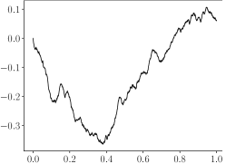
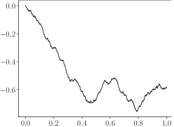
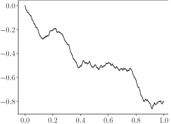
Figure 3. Three fractional Brownian motions $B_{.8}^{(1)}$, $B_{.8}^{(2)}$, and $B_{.8}^{(3)}$.

Let $f:[0,1]^{3}\rightarrow\mathbb{R}$ be defined by

(23) $$f(x_{1},x_{2},x_{3})=B_{.8}^{(1)}(x_{1})B_{.8}^{(2)}(x_{2})B_{.8}^{(3)}(x_{3}),$$

for $(x_{1},x_{2},x_{3})\in[0,1]^{3}$. Recall from the discussion in §1.2 that a tensor product of $\alpha$-Hölder continuous functions on $[0,1]^{d}$ is an $\alpha$-mixed Hölder function on $[0,1]^{d}$. Since the fractional Brownian motions $B_{.8}^{(1)}(x_{1})$, $B_{.8}^{(2)}(x_{2})$, and $B_{.8}^{(3)}(x_{3})$ are each almost surely $\alpha$-Hölder continuous for $\alpha=.79$, it follows that the function $f(x_{1},x_{2},x_{3})$ is almost surely $\alpha$-mixed Hölder for the same value of $\alpha$.

For the numerical experiments, we set $c_{1}=3.5$ and sample $\sim c_{1}\frac{1}{\varepsilon}(\log\frac{1}{\varepsilon})^{3}$ points uniformly at random from $[0,1]^{3}$, where $\varepsilon=2^{-m}$ for a given scale $m$. By sampling the function at these random points, and using the algorithm detailed in §5.1 and §5.2 we can construct an approximation $\tilde{f}$ that satisfies

$$\|f-\tilde{f}\|_{L^{2}}\lesssim\varepsilon^{\alpha}(\log\textstyle{\frac{1}{\varepsilon}})^{5/2},$$

with probability at least $1-\varepsilon^{2}$, see Theorem 1.1. For the numerical experiments we estimate $\|f-\tilde{f}\|_{L^{2}}$ by using a random test set. In particular, we sample $N=10^{8}$ points $Y_{1},\ldots,Y_{N}$ chosen independently and uniformly at random from $[0,1]^{3}$, and defined $F:=(f(Y_{1}),\ldots,f(Y_{N}))\in\mathbb{R}^{N}$, $\tilde{F}=(\tilde{f}(Y_{1}),\ldots,\tilde{f}(Y_{N}))\in\mathbb{R}^{N}$, and

$$\text{err}_{2}:=\frac{\|F-\tilde{F}\|_{2}}{\|F\|_{2}},$$

which can be viewed as a Monte Carlo approximation of the true relative error. It will also be interesting to consider the maximum relative error on the test set, which we define by

$$\text{err}_{\infty}:=\frac{\|F-\tilde{F}\|_{\infty}}{\|F\|_{\infty}}.$$

Finally, by taking advantage of the product structure of $f$, we can compute the integral $I$ of $f$ exactly. Let $\text{err}_{\text{int}}=|I-\tilde{I}|/|I|$, where $\tilde{I}$ denotes the integral of our approximation $\tilde{f}$, which can be efficiently computed as described in §1.1. We run the described numerical experiment for scales $m=5,\ldots,18$ and report the values of $\text{err}_{2}$, $\text{err}_{\infty}$ and $\text{err}_{\text{int}}$ in Table 1.

$$\begin{array}[]{c|c|c|c}m&\text{err}_{2}&\text{err}_{\infty}&\text{err}_{\text{int}}\\ \hline\cr 5&2.1515E-01&2.8048E-01&1.1245E-02\\ 6&1.3670E-01&2.1546E-01&2.4038E-03\\ 7&9.1350E-02&1.5278E-01&2.7133E-04\\ 8&5.7977E-02&1.0867E-01&1.8701E-03\\ 9&3.6125E-02&6.8297E-02&3.1067E-04\\ 10&2.2403E-02&4.1824E-02&1.2265E-06\\ 11&1.3948E-02&3.6635E-02&2.9395E-05\\ 12&8.5529E-03&2.1643E-02&4.3197E-05\\ 13&5.2153E-03&1.6592E-02&1.2824E-05\\ 14&3.1656E-03&1.1169E-02&4.7572E-06\\ 15&1.9084E-03&6.7382E-03&1.1496E-06\\ 16&1.1459E-03&4.4197E-03&1.8777E-06\\ 17&6.8489E-04&2.3634E-03&3.5733E-07\\ 18&4.0723E-04&1.5863E-03&5.3804E-08\end{array}$$

Table 1. Approximation errors for scales $m=5,\ldots,18$.

To provide context for the results reported in Table 1 we make two plots in Figure 4. On the left, we plot $\text{err}_{2}$ and $\text{err}_{\infty}$ along with two reference curves: first, we plot $\sim\varepsilon^{\alpha}(\log\frac{1}{\varepsilon})^{5/2}$, which is the upper bound from Theorem 1.1 that holds with probability at least $1-\varepsilon^{2}$. Second, we plot $\sim\varepsilon^{\alpha}$ which is approximately the amount that fractional Brownian motion with parameter $h=.8$ varies on an interval of length $\varepsilon$, which provides a lower bound, see Figure 4.

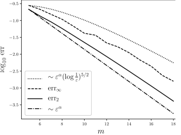
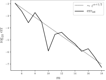
Figure 4. Visualization of data in Table 1 with references lines

The numerical results suggest that the power on $\log\frac{1}{\varepsilon}$ in Theorem 1.1 can be improved, and suggest that a similar approximation result may hold in $L^{\infty}$.

In the right plot in Figure 4, we plot $\text{err}_{\text{int}}$ along with the reference curve $\sim\varepsilon^{\alpha+1/2}$, which we suspect is the expected value of $\text{err}_{\text{int}}$ up to factors of $\log\frac{1}{\varepsilon}$. A heuristic justification for the additional factor of $\varepsilon^{1/2}$ is that computing the integral involves summing $\sim\frac{1}{\varepsilon}$ entries of the vector $w_{n}^{*}$, which we might expect to have somewhat independent errors. However, these errors are not statistically independent due to their interaction in the iteration of the Kaczmarz algorithm.

6. Discussion

In this paper, we developed a framework for synthesizing mixed Hölder functions on $[0,1]^{d}$ from random samples of the function. Our principle analytical tool is the embedding $\Psi:[0,1]^{d}\rightarrow\mathbb{R}^{p}$ that encodes the dyadic boxes of measure at least $2^{-m}$ that contain a point. This embedding allows us to consider a random sample of points $X_{1},\ldots,X_{n}\in[0,1]^{d}$ as a random matrix $\left(\Psi(X_{1})\cdots\Psi(X_{n})\right)\in\mathbb{R}^{p\times n}$. This encoding together with the randomized Kaczmarz algorithm provides a high probability approximation method for mixed Hölder functions. This method can be viewed as constructing a representation of a mixed Hölder function in a tensor Haar wavelet expansion, which can be viewed as a local product representation of a function. Product decompositions are common in the field of data analysis as a way to represent matrices and tensors, for example, the singular value decomposition represents a matrix as a sum of outer products of vectors $A=\sigma_{1}u_{1}v_{1}^{\top}+\cdots+\sigma_{k}u_{k}v_{k}^{\top}.$ Part of the larger goal of this paper is to understand how a function can be decomposed and represented as a sum of local product structures. Recall that the class of mixed Hölder functions is defined by the geometric condition that the mixed difference with respect to each box is bounded by the measure of the box to a fixed power $|\delta_{R}f|\lesssim|R|^{\alpha}$. This geometric condition is well-defined for Banach space valued functions defined on a product of metric spaces. For example, if metrics can be constructed on the rows and columns of a matrix, or similarly on each of the dimensions of a tensor, then it is possible to consider the class of mixed Hölder matrices or mixed Hölder tensors with respect to the given metrics; this approach to matrix and tensor analysis was initiated by Coifman and Gavish [3, 4] and has been developed by several authors including [1, 9, 10, 11, 16]. The results of this paper for mixed Hölder functions in the classical setting may provide insight for the development of methods to represent or complete matrices or tensors. Moreover, in the classical setting, it may be possible to generalize the results of this paper to functions with higher levels of regularity. By considering mixed Hölder functions rather than functions with higher levels of regularity, we were able to use tensor Haar wavelets rather than wavelets with more regularity; this simplified our analysis and helped to isolate the underlying geometric issues. If a function has more regularity, say, if the derivative of a function is mixed Hölder, then it may be possible to develop a similar approach to that described in this paper using tensor wavelets with more regularity to achieve better error rates.

Acknowledgements

The author would like to thank Ronald R. Coifman for many useful discussions.

References

• [1] Jerrod Ankenman and William Leeb, Mixed Hölder matrix discovery via wavelet shrinkage and Calderón-Zygmund decompositions, Appl. Comput. Harmon. Anal. 45 (2018), no. 3, 551–596. MR 3842646
• [2] Hans-Joachim Bungartz and Michael Griebel, Sparse grids, Acta Numer. 13 (2004), 147–269. MR 2249147
• [3] Ronald R. Coifman and Matan Gavish, Harmonic analysis of digital data bases, Wavelets and multiscale analysis, Appl. Numer. Harmon. Anal., Birkhäuser/Springer, New York, 2011, pp. 161–197. MR 2789162
• [4] Matan Gavish and Ronald R. Coifman, Sampling, denoising and compression of matrices by coherent matrix organization, Appl. Comput. Harmon. Anal. 33 (2012), no. 3, 354–369. MR 2950134
• [5] Thomas Gerstner and Michael Griebel, Numerical integration using sparse grids, Numer. Algorithms 18 (1998), no. 3-4, 209–232. MR 1669959
• [6] Michael Griebel and Jan Hamaekers, Fast discrete Fourier transform on generalized sparse grids, Sparse grids and applications—Munich 2012, Lect. Notes Comput. Sci. Eng., vol. 97, Springer, Cham, 2014, pp. 75–107. MR 3693086
• [7] S. Knapek and F. Koster, Integral operators on sparse grids, SIAM J. Numer. Anal. 39 (2001/02), no. 5, 1794–1809. MR 1885717
• [8] N. F. Marshall, Approximating mixed Hölder functions using random samples, arXiv e-print, (2018).
• [9] G. Mishne, R. R. Coifman, M. Lavzin, and J. Schiller, Automated cellular structure extraction in biological images with applications to calcium imaging data, bioRxiv e-print, (2018).
• [10] Gal Mishne, Ronen Talmon, Israel Cohen, Ronald R. Coifman, and Yuval Kluger, Data-driven tree transforms and metrics, IEEE Trans. Signal Inform. Process. Netw. 4 (2018), no. 3, 451–466. MR 3843472
• [11] G. Mishne, R. Talmon, R. Meir, J. Schiller, U. Dubin and R. R. Coifman, Hierarchical Coupled Geometry Analysis for Neuronal Structure and Activity Pattern Discovery, IEEE Journal of Selected Topics in Signal Processing, 10 (2016) no. 7:1238–1253.
• [12] Deanna Needell, Randomized Kaczmarz solver for noisy linear systems, BIT 50 (2010), no. 2, 395–403. MR 2640019
• [13] S. A. Smolyak. Quadrature and interpolation formulas for tensor products of certain classes of functions. Dokl. Akad. Nauk SSSR, 148(5):1042–1045, 1963.
• [14] Thomas Strohmer and Roman Vershynin, A randomized Kaczmarz algorithm with exponential convergence, J. Fourier Anal. Appl. 15 (2009), no. 2, 262–278. MR 2500924
• [15] Jan-Olov Strömberg, Computation with wavelets in higher dimensions, Proceedings of the International Congress of Mathematicians, Vol. III (Berlin, 1998), no. Extra Vol. III, 1998, pp. 523–532. MR 1648185
• [16] Or Yair, Ronen Talmon, Ronald R. Coifman, and Ioannis G. Kevrekidis, Reconstruction of normal forms by learning informed observation geometries from data, Proc. Natl. Acad. Sci. USA 114 (2017), no. 38, E7865–E7874. MR 3708297