Mobile Sensor Networks:
Bounds on Capacity and Complexity of Realizability

Abstract

We develop the mathematical theory of a model, constructed by C. Gu, I. Downes, O. Gnawali, and L. Guibas, of networks that diffuse continuously acquired information from mobile sensor nodes. We prove new results on the maximum, minimum, and expected capacity of their model of combinatorial and geometric mobile sensor networks, as well as modified versions of these models. We also give complexity results for the problem of deciding when a combinatorial mobile sensor network is generated from a geometric mobile sensor network.

A more detailed description of the concerned concepts is the following. In a restricted combinatorial mobile sensor network (RCMSN), there are $n$ sensors that continuously receive and store information from outside. Every two sensors communicate exactly once, and at an event when two sensors communicate, they receive and store additionally all information the other has stored. In a geometric mobile sensor network (GMSN), a type of RCMSN, the sensors move with constant speed on a straight line and communicate whenever a pair meet. For the purpose of analysis, all information received by two sensors before a communication event and after the previous communication events for each of them is collected into one information packet, and the capacity is defined as the ratio of the average number of sensors reached by the packets and the total number of sensors.

Contents

Introduction	1
Geometric MSNs and Restricted
Combinatorial MSNs	3
Main Results for Restricted
Geometric MSNs	5
Restricted Geometric
MSNs with Three Slopes	8
Restricted Geometric
MSNs with Four Slopes	12
Complexity of Deciding Realizability
of (R)CMSNs as (R)GMSNs	19
Future Work, Acknowledgement,
and References	24

Introduction

Following paper [1], we consider $n$ sensors that continuously receive and and store information from outside (the source is irrelevant to the model). At a communication event of two sensors, they receive additionally all information the other has stored. In this paper we study combinatorial mobile sensor networks (CMSN, proposed in [1]), in which the communication events and their order are to be specified. In order to evaluate the capacity of information diffusions in a CMSN, the authors of paper [1] collected into an information packet all information received by a sensor between two successive communication events, and merged the information packets from the two sensors at a communication event, as after the event all the information in the packet always goes together. Thus, if there are $k$ communcation events in total, then $k$ information packets are generated. In an ideal situation, all sensors receive all packets eventually. So the capacity is defined in [1] as the ratio of the actual number of packet deliveries and $kn$, or more rigorously as the following.

Definition 1 ((R)CMSN).

A restricted combinatorial mobile sensor network (RCMSN) of $n$ sensors, numbered by $1,2,\ldots,n$, is a sequence of $\binom{n}{2}$ distinct packets, which are two-element sets $\{x,y\}$ where $1\leq x<y\leq n$.

If we denote this sequence by $a_{1},\ldots,a_{n(n-1)/2}$, then we say that a packet $a_{k_{1}}$ can reach sensor $x$ ($1\leq x\leq n$), or that there is a delivery from $a_{k_{1}}$ to $x$, if there exist $1<k_{2}<\cdots<k_{m}\leq\binom{n}{2}$ such that $k_{2}>k_{1}\geq 1$, $a_{k_{j}}\cap a_{k_{j-1}}\neq\emptyset$ for each $2\leq j\leq m$, and $x\in a_{k_{m}}$. We say $a_{k_{1}}$ reaches $x$ in $m-1$ hops if $m$ is the minimum number that makes this condition hold.

A combinatorial mobile sensor network (CMSN) is like an RCMSN, except that the length $L$ of the sequence is arbitrary and the packets may be the same.

Definition 2 (Capacity of (R)CMSN).

If the length of an RCMSN or CMSN of $n$ sensors is $L$ (we clearly have $L=\binom{n}{2}$ for an RCMSN), we define the capacity of the RCMSN or CMSN to be

$$\frac{1}{nL}\sum_{k=1}^{L}\#\{1\leq x\leq n\mid a_{k}\text{ can reach }x\}.$$

To provide a comparison with RCMSN, we define the absolute capacity of a CMSN to be

$$\frac{1}{n\binom{n}{2}}\sum_{k=1}^{L}\#\{1\leq x\leq n\mid a_{k}\text{ can reach }x\}.$$

We also study a specific type of RCMSN, also proposed in [1], where the sensors move with constant speed on a straight line and communicate whenever a pair meet. On a time-position diagram, each sensor is represented by a line and each communication event by an intersection. The rigorous definition is the following.

Definition 3 (GMSN).

A geometric mobile sensor network (GMSN) of $n$ sensors is an RCMSN of $n$ sensors such that there exist $n$ lines on a Euclidean plane where each line has a finite and distinct slope, no two intersections have the same $x$-coordinate, and the RCMSN is given by sorting $\{\{i,j\}\mid 1\leq i<j\leq n\}$ according to the $x$-coordinate of the intersection between line $i$ and line $j$ in ascending order.

A variant of the GMSN is restricted GMSN (RGMSN), in which the number of slopes (i.e. speeds of sensors) is limited:

Definition 4 (RGMSN).

A restricted geometric mobile sensor network (RGMSN) of $n$ sensors and $k$ slopes is a CMSN of $n$ sensors such that there exist $n$ lines on an Euclidean plane with at most $k$ distinct slopes, all of them finite, where no two intersections have the same $x$-coordinate, and the CMSN is given by sorting $\{\{i,j\}\mid\text{line $i$ and line $j$ intersect}\}$ according to the $x$-coordinate of the intersection between line $i$ and line $j$ in ascending order.

For random geometric MSNs, the authors of [1] found that the expected capacity does not approach one when the length approaches infinity; instead, it is between $2/3$ and $5/6$. One of our main results is that the expected capacity of a random GMSN when the size approaches infinity is exactly $5/6$, improving their result.

Theorem 8 (Expectation for GMSN). If $(a_{k},b_{k})$ for $1\leq k\leq n$ are chosen independently and uniformly from $[a^{-},a^{+}]\times[b^{-},b^{+}]$, and we form a GMSN where the line representing the $k$th sensor is $y=a_{k}x+b_{k}$, then the expected capacity of the GMSN approaches $5/6$ as $n\to\infty$.

Following the suggestion by the author of [2], in this paper we also study the restricted GMSNs. We have found the asymptotic formula for the maximum possible capacity of RGMSNs with any given number of slopes.

Theorem 13 (RGMSN Max. Capacity). The maximum capacity of an RGMSN of $n$ sensors and $s\geq 3$ slopes is

$$\begin{cases}1-\frac{s-2}{s-3}n^{-1}+\Theta(n^{-2})&s\geq 4,\\ 1-n^{-1/2}+\frac{9}{8}n^{-1}+\Theta(n^{-3/2})&s=3.\end{cases}$$

Our other results on RGMSNs include the maximum absolute capacity of RGMSNs with any given number of slopes, and the exact expressions of the maximum possible capacity and the expected capacity (with lines chosen in a way similar to Theorem X) of RGMSNs with a given number $s\leq 4$ of slopes.

For random RCMSNs, we note an error of [1], pointed out by [2], and propose a conjecture that would fill the gap if proven. Also, we give new simpler proofs of the maximum and minimum possible capacities of RCMSNs, also proposed by Geneson [2], which coincide with the maximum and minimum capacity of geometric MSNs.

Finally, we consider a new question about whether a given RCMSN or CMSN can be “realized” as a GMSN or RGMSN with a given number of slopes. The other main result of this paper concerns about the complexity of algorithms deciding this realizability.

Theorem 21 (GMSN Realizability Problem). Given an RCMSN, deciding if it is generated from a GMSN is NP-Hard.

Theorem 22 (RGMSN Realizability Problem). For any fixed positive integer $s$, there is an algorithm with polynomial complexity with respect to the number of sensors for deciding whether a given CMSN is generated from an RGMSN with at most $s$ slopes.

Geometric MSNs and Restricted Combinatorial MSNs

We first consider the minimum capacity of RCMSNs. We use the idea in [1].

Theorem 5 (RCMSN/GMSN Min. Capacity [2]).

The minimum possible capacity of an RCMSN or GMSN with $n$ sensors is $2(n+1)/(3n)$.

Proof.

Clearly, any packet $\{i,j\}$ can reach both $i$ and $j$, resulting in $2\binom{n}{2}$ deliveries. Any ordering of three packets whose union contains only three distinct elements can always be expressed as $\{i,j\},\{j,k\},\{k,i\}$ in this order for distinct $i,j,k$. Here $\{i,j\}$ can reach $k$ and $\{j,k\}$ can reach $i$, resulting in $2\binom{n}{3}$ deliveries. Therefore the minimum capacity is at least

$$\frac{2\binom{n}{2}+2\binom{n}{3}}{n\binom{n}{2}}=\frac{2(n+1)}{3n}.$$

Consider the lines $l_{k}:kx+(n+1-k)y=k(n+1-k)$ for $1\leq k\leq n$. It can be verified that if $\max\{i,j\}<k$, then $\{i,j\}$ cannot reach line $k$, so the capacity of this GMSN is at most

$$\frac{1}{n\binom{n}{2}}\sum_{k=1}^{n}k(k-1)=\frac{2(n+1)}{3n}.$$

Therefore the exact minimum capacity is $\frac{2(n+1)}{3n}$. ∎

Now we consider the maximum capacity of RCMSNs. The idea is to consider those clearly unreachable sensors, and to construct a GMSN with those the only unreachable sensors.

Theorem 6 (RCMSN/GMSN Max. Capacity [2]).

The maximum possible capacity of an RCMSN or GMSN with $n$ sensors is $1-1/n+2/n^{2}$.

Proof.

Let the sequence of packets be $\{a_{1},b_{1}\},\{a_{2},b_{2}\},\ldots,\{a_{m},b_{m}\}$ where $m=\binom{n}{2}$. If a graph is formed with vertices $\{1,\ldots,n\}$ and undirected edges $(a_{k},b_{k})$, $(a_{k+1},b_{k+1})$, …, $(a_{m},b_{m})$, then the connected component containing $(a_{k},b_{k})$ has at most $m-k+1$ edges and thus at most $m-k+2$ vertices. Therefore, $\{a_{k},b_{k}\}$ can reach at most $m-k+2$ sensors for $k\geq m-n+2$, and the total number of deliveries of a GMSN is no more than

$$\sum_{k=1}^{m-n+2}n+\sum_{k=m-n+3}^{m}(m-k+2)=n(m-n+2)+\frac{n^{2}-n-2}{2}=\frac{(n-1)(n^{2}-n+2)}{2}.$$

So the maximum capacity is at most

$$\frac{(n-1)(n^{2}-n+2)/2}{n^{2}(n-1)/2}=1-1/n+2/n^{2}.$$

Now we place $n-2$ nonvertical and pairwise nonparallel lines randomly, put a line with a slope less than the minimum slope of the previous $n-2$ lines to the right of all previous intersections, and then put a line with a slope greater than the maximum of the previous $n-1$ lines to the right of all previous intersections. Then every intersection of the first $n-1$ lines obviously can reach all lines, and the last $n-1$ intersections can reach, from left to right, $n,n-1,\ldots,2$ lines. This GMSN reaches our upper bound. ∎

In this proof, the construction used is called a collector-distributor construction [1, 2]. Similar constructions will be used in the next section.

What about the expected capacity of RCMSNs? It is claimed in [1] that the expected capacity of an RCMSN with $n$ sensors is $1-O(\log^{2}n/n)$. However, their proof is incorrect [2]. They partitioned the $\binom{n}{2}$ communications into groups of size $\lceil n\log n\rceil$, found that the probability that all $n$ sensors appear in one given group is more than $1-1/n$, and concluded that with high probability, all groups contain all $n$ sensors. But this is not true as the events of a sensor appearing in the groups are not independent. In order for their argument to hold, the following conjecture must be proven.

Conjecture 7.

If all pairs $(i,j)$ where $1\leq i<j\leq n$ are partitioned into groups of size $\lceil n\log n\rceil$, an expected proportion $1-O(\log n/n)$ of the groups contain all numbers $1,\ldots,n$.

In [1] it is also showed that the expected capacity of a random GMSN is no more than $5/6$ when the network size approaches infinity, considering some lines with high or low slopes that clearly cannot be reached by intersections in certain regions. Here, we improve the result by directly computing the expected capacity using Wolfram Mathematica.

Theorem 8 (Expectation for GMSN).

If $(a_{k},b_{k})$ for $1\leq k\leq n$ are chosen independently and uniformly from $[a^{-},a^{+}]\times[b^{-},b^{+}]$, and we form a GMSN where the line representing the $k$th sensor is $y=a_{k}x+b_{k}$, then the expected capacity of the GMSN approaches $5/6$ as $n\to\infty$.

Proof.

By applying scaling, shear transformation, and translation, we may assume that $a^{-}=b^{-}=0$ and $a^{+}=b^{+}=1$ without changing the probability of each possible GMSN’s capacity, because the order of two consecutive disjoint communications does not affect the capacity. The process of randomly choosing $n$ lines can also be considered as the following process: first randomly choose two lines $l:y=ax+b$ and $l^{\prime}:y=a^{\prime}x+b^{\prime}$, then randomly choose a set $A$ of $\sqrt{n}$ lines, then randomly choose a set $B$ of $n-\sqrt{n}-2$ lines. We count the number of triples $(\{u,v\},w)$ of lines, among all $n\binom{n}{2}$ such triples, such that $u\cap v$ can reach $w$. Theorem 3.4 in [1] shows that exactly $2\binom{n}{2}+2\binom{n}{3}$ triples satisfy that $u\cap v$ can reach $w$ in at most one hop. Theorem 3.8 in [1] states that at most two hops are required for any delivery in a GMSN, so we need only count the expected number of triples where $u\cap v$ can and only can reach $w$ in exactly two hops.

By linearity of expectation, we need only count the number of such triples $(\{u,v\},w)$ when $\{u,v\}=\{l,l^{\prime}\}$. In fact, we count only those triples where $w\in B$, because we need only prove that the expected capacity is $\geq 5/6$ (as Theorem 3.5 in [1] shows it is $\leq 5/6$). Because $l$ and $l^{\prime}$ can be swapped, we shall assume that $a^{\prime}>a$ and multiply the result under this condition by 2.

Now $(a,b)$ is chosen uniformly at random from $[0,1]\times[0,1]$, then $(a^{\prime},b^{\prime})$ is chosen uniformly at random from $[a,1]\times[0,1]$. If a line $y=a^{\prime\prime}x+b^{\prime\prime}$ in $A$ has a slope higher than $a^{\prime}\geq a$ and can be reached by $l\cap l^{\prime}$, then we have $0\leq b^{\prime\prime}<\max\{0,\min\{1,b+(b^{\prime}-b)(a-a^{\prime\prime})/(a-a^{\prime})\}\}$. Thus a proportion of

$$2\int_{0}^{1}\int_{0}^{1}\int_{a}^{1}\int_{0}^{1}\int_{a^{\prime}}^{1}\max\bigg{\{}0,\min\bigg{\{}1,b+(b^{\prime}-b)\cdot\frac{a-a^{\prime\prime}}{a-a^{\prime}}\bigg{\}}\bigg{\}}\,\mathrm{d}a^{\prime\prime}\,\mathrm{d}b^{\prime}\,\mathrm{d}a^{\prime}\,\mathrm{d}b\,\mathrm{d}a=\frac{1}{6}$$

of the lines in $A$ has such properties. Among these lines, the line $l^{*}$ with the maximum slope is expected to have slope equal to the upper limit of its possible range when $|A|=\sqrt{n}\to\infty$. This upper limit is 1 if $l\cap l^{\prime}$ is not in the first quadrant (equivalently, $b^{\prime}>b$), and $\min\{1,\text{slope}(\overline{(0,0)(l\cap l^{\prime})}))$ otherwise.

So we divide into the cases of $b^{\prime}>b$ and $b^{\prime}<b$ when counting the number of lines $y=a^{\prime\prime}x+b^{\prime\prime}$ in $B$ that: have slope higher than $a^{\prime}\geq a$; cannot be reached by $l\cap l^{\prime}$ in at most one hop (equivalently, $\max\{0,\min\{1,b+(b^{\prime}-b)(a-a^{\prime\prime})/(a-a^{\prime})\}\}<b^{\prime\prime}\leq 1$); and can be reached by $l\cap l^{\prime}$ in two hops via $l^{*}$ (equivalently, $a^{\prime\prime}$ is less than the expected slope of $l^{*}$ discussed above). A proportion of

$$2\int_{0}^{1}\int_{0}^{1}\int_{a}^{1}\bigg{(}\int_{b}^{1}\int_{a^{\prime}}^{1}+\int_{0}^{b}\int_{a^{\prime}}^{\min\{1,\frac{a^{\prime}b-ab^{\prime}}{b-b^{\prime}}\}}\bigg{)}\\ \max\bigg{\{}0,\min\bigg{\{}1,1-b-(b^{\prime}-b)\cdot\frac{a-a^{\prime\prime}}{a-a^{\prime}}\bigg{\}}\bigg{\}}\,\mathrm{d}a^{\prime\prime}\,\mathrm{d}b^{\prime}\,\mathrm{d}a^{\prime}\,\mathrm{d}b\,\mathrm{d}a=\frac{1}{12}$$ (1)

of the lines in $B$ has such properties.

We can do a similar reasoning for lines with slope lower than that of both $l$ and $l^{\prime}$. Thus for every randomly chosen two lines $l$ and $l^{\prime}$, at least $(n-\sqrt{n}-2)/6$ triples $(\{l,l^{\prime}\},l^{\prime\prime})$ require exactly two hops. Therefore in total it is expected that $\geq\binom{n}{2}(n-\sqrt{n}-2)/6$ triples require exactly two hops, so the expected capacity is greater than

$$\frac{2\binom{n}{2}+2\binom{n}{3}+\binom{n}{2}(n/6+o(n))}{n\binom{n}{2}}=\frac{5}{6}+o(1).$$

∎

Although we know the capacity of GMSNs with size approaching infinity, how concentrated they are is still left open.

Question 9.

What is the variance of the capacity of a GMSN with $n$ sensors when $n\to\infty$?

Main Results for Restricted Geometric MSNs

Next, we consider the bounds on the capacity of RGMSNs. Clearly, the minimum capacity of any RGMSN is zero because we can always make all lines parallel. So we only find the maximum capacities. When limited to only two slopes, the geometric form of any RGMSN is a grid, so the capacity can be directly computed and is also easy, as shown by the following theorem.

Proposition 10 (2-Slope RGMSN Max. Capacity).

The capacity for any RGMSN of $n$ sensors and 2 slopes is $\frac{n+1}{2n}$. The maximum and expected absolute capacities of an RGMSN of $n$ sensors and 2 slopes are $\frac{n+2}{4n-4}$ and

$$\begin{cases}\frac{n+2}{4n}&n\text{ is even}\\ \frac{(n+1)(n+2)}{4n^{2}}&n\text{ is odd}\end{cases},$$

respectively.

Proof.

Suppose there are $m$ lines with the larger slope and $n-m$ lines with the smaller slope. Without loss of generality, suppose all slopes are positive. We order the lines with the larger slope by their $x$-intercepts from the largest to smallest and label them $a_{1},a_{2},\ldots,a_{m}$, and order and label the lines with the smaller slope in the same way as $b_{1},b_{2},\ldots,b_{n-m}$. Clearly, the intersection $a_{i}\cap b_{j}$ can reach lines $a_{1},\ldots,a_{i}$ and $b_{1},\ldots,b_{j}$ but no other lines. Therefore, the capacity of the RGMSN is

$$\frac{1}{nm(n-m)}\sum_{i=1}^{m}\sum_{j=1}^{n-m}(i+j) =\frac{1}{nm(n-m)}\cdot\bigg{(}(n-m)\bigg{(}\sum_{j=1}^{m}j\bigg{)}+m\bigg{(}\sum_{j=1}^{n-m}j\bigg{)}\bigg{)}$$

$$=\frac{1}{2}+\frac{1}{n}.$$

The absolute capacity of the RGMSN is

$$\frac{m(n-m)}{\binom{n}{2}}\bigg{(}\frac{1}{2}+\frac{1}{n}\bigg{)}=\frac{m(n-m)(n+2)}{n^{2}(n-1)},$$

which clearly has maximum given in the theorem statement and expected value

$$2^{-n}\sum_{m=0}^{n}\binom{n}{m}\frac{m(n-m)(n+2)}{n^{2}(n-1)}=2^{-n}\cdot\frac{n+2}{n}\sum_{m=1}^{n-1}\binom{n-2}{m-1}=\frac{n+2}{4n}.$$

∎

Remark 11.

In proofs that follow, a grid will mean a collection of lines with exactly two distinct slopes. Sometimes, we explicitly give the slopes $k_{1},k_{2}$ and say a $k_{1}$-$k_{2}$ grid.

When there are three or more slopes, we can use a strategy similar to that in Theorem 6: trying to find as many unreachable lines as possible, and finding an example that attains the upper bound. While Theorem 6 only considers the last $n-1$ intersections, we need to consider the lines with the largest and smallest slopes when the number of slopes is limited.

We first deal with the easier one, absolute capacity, where the maximum is asymptotically less than one:

Proposition 12 (RGMSN Max. Abs. Capacity).

The maximum absolute capacity of an RGMSN of $n$ sensors and $s\geq 3$ slopes is, when $n\to\infty$,

$$\frac{(135s^{3}-945s^{2}+2232s-1796)+4(9s^{2}-42s+52)^{3/2}}{243(s-2)^{3}}.$$

Proof.

We consider the intersections that lie on the $a$ lines with the highest slope $k$ and the $b$ lines with the lowest slope $k^{\prime}$. For a line whose slope is not equal to $k$ or $k^{\prime}$, every intersection of it with a line with slope $k$ or $k^{\prime}$ cannot any lines with slopes $k$ or $k^{\prime}$ to the left of it because of the maximality and minimality of $k$ and $k^{\prime}$ (for if it reaches a line to the left, it can only do so via a line with higher absolute value of slope; but there are no such lines). Thus, for each of these $n-a-b$ lines, the intersections mentioned above cannot reach at least $1+2+\cdots+(a+b-1)$ lines in total. For intersections of the lines with slopes $k$ or $k^{\prime}$, the total number of lines they cannot reach is at least $(0+1+\cdots+(b-1))+(1+2+\cdots+b)+\cdots+((a-1)+a+\cdots+(a+b-2))$.

Suppose the slopes other than $k$ and $k^{\prime}$ are $k_{1},\ldots,k_{s-2}$, and the corresponding numbers of lines are $c_{1},\ldots,c_{s-2}$, respectively. Then the total number of information deliveries is at most

$$n\bigg{(}ab+(a+b)\sum_{j=1}^{s-2}c_{j}+\sum_{i\neq j}c_{i}c_{j}\bigg{)}-(n-a-b)\sum_{j=1}^{a+b-1}j-\sum_{i=0}^{a-1}\sum_{j=0}^{b-1}(i+j).$$

This is maximized when all the $c_{j}$’s are equal and $a=b$; after that, we have only one free variable in the sum:

$$f(a)=n\bigg{(}a^{2}+2a(n-2a)+\frac{(s-2)(s-3)}{2}\bigg{(}\frac{n-2a}{s-2}\bigg{)}^{2}\bigg{)}-(n-2a)a(2a-1)-a^{2}(a-1).$$

So we found that the maximum sum divided by $n\binom{n}{2}$ is equal to the formula given in the theorem statement when $n\to\infty$. The collector-distributor construction attains this upper bound as the formulas for the total number of information deliveries are almost entirely the same as the one above. ∎

For the maximum capacity of an RGMSN, we need to consider both the largest or smallest slopes and the last $n-1$ intersections. The proof is essentially similar to that of Proposition 12.

Theorem 13 (RGMSN Max. Capacity).

The maximum capacity of an RGMSN of $n$ sensors and $s\geq 3$ slopes is asymptotically

$$\begin{cases}1-\frac{s-2}{s-3}n^{-1}+\Theta(n^{-2})&s\geq 4\\ 1-n^{-1/2}+\frac{9}{8}n^{-1}+\Theta(n^{-3/2})&s=3.\end{cases}$$

Proof.

Consider the $a$ lines with the largest slope and the $b$ lines with the smallest slope. They form a grid. Suppose, without loss of generality, that the largest slope is 1 and the smallest slope is $-1$. The intersections of lines in the grid cannot reach at least $\sum_{i=0}^{a-1}\sum_{j=0}^{b-1}(i+j)$ lines. The grid can also be seen as a set of $a+b$ curves, where the $k$th curve consists of those points on the gridlines such that there are $k-1$ gridlines on their right. Each of these curves intersects with all the remaining $n-a-b$ lines with slope $\neq\pm 1$; these intersections cannot reach at least $(n-a-b)(1+2+\cdots+(a+b-1))$ gridlines. Also, in the arrangement, the $k$th rightmost intersection obviously can reach at most $k+1$ lines (by induction), so the $n-1$ rightmost intersections cannot reach at least $1+2+\cdots+(n-2)$ lines. But we may have counted some intersections’ unreachable lines twice. At worst, we overestimated it by $(n-1)(a+b)$ unreachable lines. Therefore, the maximum capacity with only $s$ slopes is at most

$$1-\frac{(\sum_{k=1}^{n-2}k)+(n-a-b)(\sum_{k=1}^{a+b-1}k)+\sum_{i=0}^{a-1}\sum_{j=0}^{b-1}(i+j)-(n-1)(a+b)}{n(ab+(a+b)(n-a-b)+\frac{(s-2)(s-3)}{2}(\frac{n-a-b}{s-2})^{2})}.$$

To give an upper bound to this formula, we need only compute the minimum value of

$$\kappa =\frac{(\sum_{k=1}^{n-2}k)+(n-a-b)(\sum_{k=1}^{a+b-1}k)+\sum_{i=0}^{a-1}\sum_{j=0}^{b-1}(i+j)-(n-1)(a+b)}{ab+(a+b)(n-a-b)+\frac{(s-2)(s-3)}{2}(\frac{n-a-b}{s-2})^{2}}$$

$$=\frac{\frac{1}{2}(n-1)(n-2)+\frac{1}{2}(n-a-b)(a+b)(a+b-1)+\frac{1}{2}ab(a+b-2)-(n-1)(a+b)}{ab+(a+b)(n-a-b)+\frac{s-3}{2(s-2)}(n-a-b)^{2}}$$

$$=\frac{\frac{1}{2}(n-a-b-1)(n-2)-\frac{1}{2}(a+b)^{2}-\frac{1}{4}(1-\frac{1}{s-2})(a+b-2)(n-a-b)^{2}}{ab+(a+b)(n-a-b)+\frac{s-3}{2(s-2)}(n-a-b)^{2}}+\frac{a+b-2}{2}$$

When $a+b<n$ is fixed, only the $ab$ on the denominator can vary, so when $\kappa$ is minimized, either $a=b$ (when the numerator is positive) or $b=1$ (when the numerator is negative. In either case, the formula of $\kappa$ contains only one free variable, so we found that when $s\geq 4$, the minimum of $\kappa$ is either

$$\frac{(s-2)n^{2}-(5s-10)n+2s-4}{(s-3)n^{2}+4n-2s}$$

or a real root between 0 and $n$ of

$$(-(s-2)^{3}n^{5}+O(n^{4}))+((s-2)^{2}(s-3)n^{5}+O(n^{4}))t+O(n^{4})t^{2}+O(n^{3})t^{3}+O(n^{2})t^{4}=0,$$

where we have omitted small terms. Both result in an upper bound $1-\frac{s-2}{s-3}\frac{1}{n}+\Theta(n^{-2})$ of the capacity. Similar to Proposition 12, it is not difficult to compute that the collector-distributor construction attains this upper bound—the formulas are almost entirely the same.

When $s=3$, we have

$$\kappa=\frac{(n-a-b-1)(n-2)-(a+b)^{2}}{2(ab+(a+b)(n-a-b))}+\frac{a+b-2}{2},$$

which is minimized either

$$\text{when }a=b<\frac{\sqrt{5n^{2}-16n+12}-(n-2)}{4}\text{ or when }b=1\text{ and }a>\frac{\sqrt{5n^{2}-16n+12}-n}{2}.$$

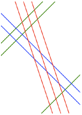
Figure 1: An RGMSN of 3 slopes. There are $a=3$ red lines, $a=3$ green lines, and $b=2$ blue lines here.

In each case, the formula then has only one variable and an upper bound of the capacity is $1-n^{-1/2}+\frac{9}{8}n^{-1}+\Theta(n^{-3/2})$. (We omit the actual maximum value due to its length.) However, the collector-distributor construction does not attain the bound here. That is because unlike the previous cases, neither $a$ nor $b$ is $O(1)$ when the capacity formula is maximized. Instead, we use the following construction. Let $1\leq a\leq\lfloor(n-1)/2\rfloor$ be an integer whose value will be determined later, and $b=n-2a$. In $\mathbb{R}^{2}$ we draw the $b$ lines $y=k$ ($0\leq k\leq b-1$), the $a-1$ lines $x=k$ ($1\leq k\leq a-1$), the $a$ lines $x+2y=a+2(b+k)-3$ ($1\leq k\leq a$), and the line $x=3a+2b$, and rotate all lines by $\pi/4$ clockwise about the origin (Fig. 1). Then we get an RGMSN with 3 slopes whose capacity is

$$\frac{1}{n(a^{2}+2ab)}\bigg{(}\sum_{k=2}^{b+1}k+(b+1)\sum_{k=b+2}^{a+b+1}k+(a-1)\sum_{k=b+2}^{a+b+1}k+a\sum_{k=1}^{a-1}k+b\sum_{k=a+b+2}^{2a+b}k\bigg{)}$$

$$=\frac{a+b+1}{n}-\frac{n-1}{2n}\frac{b}{a^{2}+2ab}=:f(a,b).$$

This can attain the upper bound (computed with differential calculus) $1-n^{-1/2}+\frac{9}{8}n^{-1}+\Theta(n^{-3/2})$ we found when $a$ is allowed to be non-integers. When $a$ must be an integer, the deviation from the upper bound is at most

$$\max_{0\leq t\leq 1}\{f(a^{\prime},b^{\prime})-f(a^{\prime}+t/2,b^{\prime}-t)\}=\frac{1}{2n\sqrt{n}}+\Theta(n^{-2}),$$

where $f(a^{\prime},b^{\prime})=\max_{1\leq a\leq(n-1)/2}f(a,b)$, so this construction attains the upper bound. ∎

Restricted Geometric MSNs with Three Slopes

Proposition 13 only gives the capacity of near-optimal constructions, not the optimal construction. We have found a method to produce optimal constructions for RGMSNs of no more than four slopes, although it does not generalize to higher numbers of slopes. We begin with RGMSNs with at most three slopes. The method is to move lines with the third slope in the “grid” formed by existing lines in two slopes.

Remark 14.

In the proofs below, a grid is a collection of lines with exactly two different slopes. A corner of a grid is an intersection from which there exists a ray that intersects no other lines in the grid. A path is a line that intersects the grid. The intersection where a path enters or leaves a grid is one next to a corner, and the former one can reach the latter one but not vice versa.

Proposition 15 (Three-Slope RGMSN Max. Capacity).

The maximum capacity of an RGMSN of $n$ sensors with only three possible slopes allowed is equal to

$$\max\bigg{\{} \frac{(4p-1)n^{2}-(10p^{2}-6p-1)n+(6p^{3}-6p^{2}-2p)}{4pn^{2}-6p^{2}n},$$

$$\frac{(4q+1)n^{2}-(10q^{2}+4q-1)n+(6q^{3}+3q^{2}-3q-2)}{(4q+2)n^{2}-(6q^{2}+6q+2)n}\bigg{\}}$$

where $q=\lfloor\sqrt{n}/2\rfloor$ and either $p=q$ or $p=q+1$. This is asymptotically $1-\frac{1}{\sqrt{n}}+\frac{9}{8n}+r_{n}n^{-3/2}$, where $\liminf_{n\to\infty}r_{n}=\frac{15}{32}$ and $\limsup_{n\to\infty}r_{n}=\frac{19}{32}$.

Remark 16.

The main results of this theorem and Proposition 18 below are constructions of the RGMSNs with maximum capacity, in contrast to Proposition 13 where only a bound is computed.

Proof.

Suppose there are $a$ lines in slope $k_{1}$, $b$ lines in slope $k_{2}$, and $c$ lines in slope $k_{3}$, where $a+b+c=n$. Without loss of generality, suppose the rightmost intersection lies on lines with slopes $k_{1}<k_{2}$. All lines with those two slopes form an $a$-by-$b$ grid. Because the order of the $x$-coordinates of the intersections depends only on differences of slopes and differences of intercepts between lines, we may replace each slope $k$ by $\frac{2}{k_{2}-k_{1}}(k-\frac{k_{1}+k_{2}}{2})$ without changing the CMSN that corresponds to the RGMSN. Thus, we may assume $k_{1}=-k_{2}=1$ without loss of generality. Also, by symmetry we may assume $k_{3}<-1$.

For convenience, we name the lines. Let $s_{1}$ be the line with slope 1 that is closest to the rightmost intersection, then let $s_{2}$ be the line with slope 1 next to $s_{1}$, and so on. Let $t_{1}$ be the line with slope $-1$ that is closest to the rightmost intersection, then let $t_{2}$ be the line with slope $-1$ next to $t_{1}$, and so on. Also, we label each intersection with the number of lines it can reach.

Now we investigate where we should put the remaining $c$ lines in between so as to maximize the capacity. In the diagrams below, in order to save space, we draw lines in the grid as straight lines, and lines with slope $k_{3}$ as paths. They represent where the added straight lines with slope $k_{3}$ are. So the paths have to enter the grid (going from infinity above) above $s_{a}\cap t_{1}$ and leave the grid below $s_{1}\cap t_{b}$ (and going to infinity below). They also intersect any grid-line exactly once (Fig. 2). Note that it may be the case that even if paths obey these rules, the resulting diagram cannot be realized as an RGMSN (with all lines straight), but we do not care about such cases now (an example can be found in Fig. 14). Instead, we only guarantee that the best arrangement can be realized.

We first find the best arrangement (with maximum capacity) when $c=1$. Here the line with slope $k_{3}$ is named $l$.

Step 1. Where should the path leave the grid?

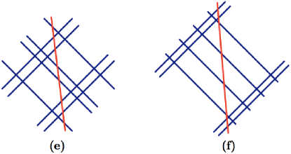
Figure 2: (a) and (b) are valid paths. Path (c) is invalid because it intersects an existing line three times. Path (d) is invalid because it contradicts the given rightmost intersection, even if it can be pulled straight. Diagrams (e) and (f) show the realizations of (a) and (b) in straight lines, respectively.

We have included a diagram ((a) and (b) in Fig. 3) to help understand the description below. Suppose we initially have a path that leaves the grid between $t_{i}$ and $t_{i+1}$ (that is, it intersects $t_{i}$, $s_{1}$, and $t_{i+1}$ in this order, as shown in (a)). Now we modify the path and make it leave the grid between $t_{i-1}$ and $t_{i}$, assuming that the path is still valid and the positions of other intersections relative to the grid are not changed. Then only the labels on $s_{1}\cap t_{i}$ and $t_{i}\cap l$ change. Other intersections are not affected because either they cannot reach $l$ and are thus unrelated to the change, or they can still travel through $l$ to the lines they previously can reach. Note that although $l\cap s_{1}$ changes its relative position to the grid, its label does not change as it can still reach $l$ and all $t_{j}$, but not other lines. The following table shows the changes in the two intersections’ labels:

Intersection	Original	Reason	New	Reason
$s_{1}\cap t_{i}$	$i+1$	it cannot reach $l$	$b+2$	it can reach all $t_{j}$ through $l$ and $s_{1}$
$t_{i}\cap l$	$b+2$	it can reach all $t_{j}$ through $l$ and $s_{1}\cap t_{i}$, plus $s_{1}$	$b-i+2$	it can reach $t_{i},\ldots,t_{b}$ through $l$

This table tells us that whether the new network has a larger capacity depends on whether $i>(b+1)/2$.

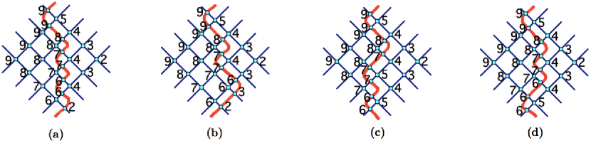
Figure 3: In (a) and (b), the place that the path leaves the grid changes; in (c) and (d), the relative position of the path and one intersection changes. When pulled straight, the new lines all have negative slope. The number of lines that can be reached from each intersection is labeled.

Step 2. Where should the path cross the grid?

Diagrams (c) and (d) in Fig. 3 are concerned here. Suppose we initially have a path that intersects $t_{i}$ and $s_{j}$ consecutively in this order ($j>1$), meaning that $l\cap t_{i}$ is to the left of $l\cap s_{j}$. Now we switch their order while leaving other intersections unchanged. Then, for reasons similar to those in the previous paragraph, only the labels on $s_{j}\cap t_{i}$ and $t_{i}\cap l$ change. All other intersections are unrelated. The following table shows the changes in the two intersections’ labels:

Intersection	Original	Reason	New	Reason
$s_{j}\cap t_{i}$	$i+j$	it cannot reach $l$	$b+j+1$	it can reach all $t_{i}$ through $l$ and $s_{j}$, and also $s_{1},\ldots,s_{j}$
$t_{i}\cap l$	$b+j+1$	it can reach all $t_{i}$ through $l$ and $s_{j}\cap t_{i}$, and also $s_{1},\ldots,s_{j}$	$b+j$	it can reach all $t_{i}$ through $l$ and $s_{j-1}\cap t_{i}$, and also $s_{1},\ldots,s_{j-1}$

This table tells us that the new network always has no less capacity.

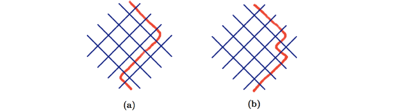
Figure 4: The best network and the second best network.

Given any valid path, one can always perform the two operations to transform it to one of the two paths shown in Fig. 4 above as follows: a path can be mapped to a string of S and T indicating at the current cell in the grid if the path crosses an $s_{j}$ to another cell or a $t_{i}$ to another cell. For example, the path in Fig. 2(a) is mapped to the string TSSTSTST. Now, the discussions above tell us that a substring TS can be replaced by ST without reducing capacity if there exists at least one S following this substring. Repeating this operation, any string can be transformed to the form SS…STT…TSTT…T. The discussions above also tell us that the last S may either be moved to the end or the beginning; one of the two choices does not reduce the capacity. Therefore any string is transformed to SS…STT…TS or SS…STSTT…T (without violating the rightmost intersection), which correspond to Fig. 4 (a) and (b) respectively.

Now we consider the case $c>1$. For the rightmost line $l$ with slope $k_{3}$, we may apply the same discussions as above to move it to one location in Fig. 4. Then, no matter how other lines with slope $k_{3}$ move, the total capacity does not change because each intersection on the left of $l$ can reach $l$, and can thus reach all the $t_{i}$’s; the intersection always can reach all the $s_{j}$’s below it and no $s_{j}$’s above it; and it always can reach all lines with slope $k_{3}$ to the right of it and none to the left. Moving a line with slope $k_{3}$ across an intersection only exchanges two intersections’ labels.

The total number of information deliveries in Fig. 4(a) is

$$\sum_{k=2}^{b+1}k+(b+1)\sum_{k=b+2}^{b+c+1}k+(a-1)\sum_{k=b+2}^{b+c+1}k+c\sum_{k=1}^{a-1}k+b\sum_{k=b+c+2}^{b+c+a}k,$$

and the total number of information deliveries in Fig. 4(b) is

$$2+c\sum_{k=1}^{b-1}k+(b-1)\sum_{k=1}^{c}k+(a+1)\sum_{k=b+2}^{b+c+1}k+c\sum_{k=1}^{a-1}k+(b-1)(b+c+1)+b\sum_{k=b+c+2}^{a+b+c}k.$$

The difference between the two sums is $(b-1)(b(c-1)+2)\geq 0$, so Fig. 4(a) has no less capacity than Fig. 4(b). The sum in Fig. 4(a) equals $((2b+a+c+1)(ab+bc+ca)+(ac+b-b^{2}))/2$, so the capacity to be maximized is

$$\frac{(2b+a+c+1)(ab+bc+ca)+(ac+b-b^{2})}{2n(ab+bc+ca)}=\frac{2b+a+c+2}{2n}-\frac{n-1}{2n}\frac{b}{ab+bc+ca}.$$

If $a$, $b$, and $c$ may be non-integers, this is maximized when $a=c=\sqrt{n}/2+O(n^{-1/2})$, so when the variables must be integers, each of $a$ and $c$ must be equal to $p$ or $p+1$ (which is defined in the theorem statement); this leads to the formula given in the theorem. For the asymptotic formula, we observe that the capacity has a maximum value equal to $1-\frac{1}{\sqrt{n}}+\frac{9}{8n}+\frac{19}{32n\sqrt{n}}+\Theta(n^{-2})$, which is achieved when $n$ is an even perfect square and $a=c=\sqrt{n}/2$, giving the limsup value. Also, when $a=c=\sqrt{n}/2-t$ is an integer, the capacity is $1-\frac{1}{\sqrt{n}}+\frac{9}{8n}+\frac{19-64t^{2}}{32n\sqrt{n}}+\Theta(n^{-2})$, and when $a=\sqrt{n}/2-t$ and $c=\sqrt{n}/2+1-t$ are integers, the capacity is $1-\frac{1}{\sqrt{n}}+\frac{9}{8n}+\frac{3-64t(t-1)}{32n\sqrt{n}}+\Theta(n^{-2})$. If $\frac{19-64t^{2}}{32}<\frac{15}{32}$ we must have $|t|>\frac{1}{4}$, and in this case $\frac{3-64|t|(|t|-1)}{32}>\frac{15}{32}$, so we always have $r_{n}\geq\frac{15}{32}$; this liminf is achieved by $n=4k^{2}+2k+1$ for positive integers $k$. ∎

Regarding RGMSNs with at most three slopes, we have also found their expected capacity for three slopes and all intercepts chosen uniformly in some interval. The idea for the proof is similar to the idea in Theorem 8 (expected capacity for GMSN)—identifying all possible terms that contribute to the capacity of the RGMSN. We note that the integrals here are also computed using Wolfram Mathematica like in Theorem 8.

Proposition 17 (Expectation for Three-Slope RGMSN).

The expected capacity of an RGMSN with at most three slopes and $n$ sensors is $11/18$ when $n\to\infty$.

Proof.

Like in Theorem 8, without loss of generality, we assume the slopes and intercepts are chosen independently and uniformly from $[0,1]$. First, we choose the three slopes, and let them be $a_{1}<a_{2}<a_{3}$ (the probability that two of them are equal is zero). Then we choose the slopes of the $n$ lines independently and uniformly from the three slopes with equal probability, and choose the intercepts of the $n$ lines independently and uniformly from $[0,1]$. Let $n_{k}$ lines have slope $a_{k}$ for $k=1,2,3$.

Let $u$ be a line $y=a_{i}x+b_{i}$, $v$ be a line $y=a_{j}x+b_{j}$, and $w$ be a line $y=a_{k}x+b_{k}$, where $1\leq i<j\leq 3$. If $k\leq i$, and $u\cap v$ can reach $w$ in one hop, then we have $(b_{i}-b_{j})/(a_{j}-a_{i})<(b_{k}-b_{j})/(a_{j}-a_{k})$, so the probability of this is

$$\frac{\displaystyle\int_{0}^{1}\int_{a_{1}}^{1}\int_{a_{2}}^{1}\int_{0}^{1}\int_{0}^{1}\min\bigg{\{}1,\max\bigg{\{}0,b_{j}+(b_{k}-b_{j})\frac{a_{j}-a_{i}}{a_{j}-a_{k}}\bigg{\}}\bigg{\}}\,\mathrm{d}b_{k}\,\mathrm{d}b_{j}\,\mathrm{d}a_{3}\,\mathrm{d}a_{2}\,\mathrm{d}a_{1}}{\displaystyle\int_{0}^{1}\int_{a_{1}}^{1}\int_{a_{2}}^{1}\,\mathrm{d}a_{3}\,\mathrm{d}a_{2}\,\mathrm{d}a_{1}}=\frac{1}{2}.$$

(Note: to compute this integral, one may use the substitution $(b_{j},b_{k})\mapsto(1-b_{j},1-b_{k})$, then the sum of the resulting formula and the original formula is clearly 1.) If $u\cap v$ can reach the leftmost line with slope $a_{l}$ where $l<k$, then it can reach $w$ in one or two hops. The probability of this is

$$\frac{\displaystyle\begin{multlined}\displaystyle\int_{0}^{1}\int_{a_{1}}^{1}\int_{a_{2}}^{1}\int_{0}^{1}\cdots\int_{0}^{1}\min\bigg{\{}1,\max\bigg{\{}0,\max_{1\leq l<k}\bigg{\{}b_{j}+(b_{l}-b_{j})\frac{a_{j}-a_{i}}{a_{j}-a_{l}}\bigg{\}}\bigg{\}}\bigg{\}}\\ \,\mathrm{d}b_{1}^{n_{1}}\ldots\,\mathrm{d}b_{k-1}^{n_{k-1}}\,\mathrm{d}b_{j}\,\mathrm{d}a_{3}\,\mathrm{d}a_{2}\,\mathrm{d}a_{1}\end{multlined}\displaystyle\int_{0}^{1}\int_{a_{1}}^{1}\int_{a_{2}}^{1}\int_{0}^{1}\cdots\int_{0}^{1}\min\bigg{\{}1,\max\bigg{\{}0,\max_{1\leq l<k}\bigg{\{}b_{j}+(b_{l}-b_{j})\frac{a_{j}-a_{i}}{a_{j}-a_{l}}\bigg{\}}\bigg{\}}\bigg{\}}\\ \,\mathrm{d}b_{1}^{n_{1}}\ldots\,\mathrm{d}b_{k-1}^{n_{k-1}}\,\mathrm{d}b_{j}\,\mathrm{d}a_{3}\,\mathrm{d}a_{2}\,\mathrm{d}a_{1}}{\displaystyle\int_{0}^{1}\int_{a_{1}}^{1}\int_{a_{2}}^{1}\int_{0}^{1}\cdots\int_{0}^{1}\,\mathrm{d}b_{1}^{n_{1}}\ldots\,\mathrm{d}b_{k-1}^{n_{k-1}}\,\mathrm{d}a_{3}\,\mathrm{d}a_{2}\,\mathrm{d}a_{1}}.$$

(Note: we have written the formulas in this form so that it generalizes to RGMSNs with more than three slopes.) When $n\to\infty$, the expected value of $n_{t}\to\infty$ for each $t$, so we found the probability when $n\to\infty$ is $1/4$ for $(i,j,k)=(2,3,2)$.

If $i<k<j$, then $u\cap v$ can always reach $w$ in one hop. If $k\geq j$, and $u\cap v$ can reach $w$ in one hop, then we have $(b_{i}-b_{j})/(a_{j}-a_{i})<(b_{k}-b_{j})/(a_{j}-a_{k})$, so the probability of this is the same as the first formula. If $u\cap v$ can reach the rightmost line with slope $a_{l}$ where $l>k$, then it can reach $w$ in one or two hops. The probability of this is

$$\frac{\displaystyle\begin{multlined}\displaystyle\int_{0}^{1}\int_{a_{1}}^{1}\int_{a_{2}}^{1}\int_{0}^{1}\int_{1}^{0}\cdots\int_{1}^{0}\min\bigg{\{}1,\max\bigg{\{}0,\max_{k<l\leq 3}\bigg{\{}b_{j}+(b_{l}-b_{j})\frac{a_{j}-a_{i}}{a_{j}-a_{l}}\bigg{\}}\bigg{\}}\bigg{\}}\\ \,\mathrm{d}(1-b_{k+1})^{n_{k+1}}\ldots\,\mathrm{d}(1-b_{3})^{n_{3}}\,\mathrm{d}b_{j}\,\mathrm{d}a_{3}\,\mathrm{d}a_{2}\,\mathrm{d}a_{1}\end{multlined}\displaystyle\int_{0}^{1}\int_{a_{1}}^{1}\int_{a_{2}}^{1}\int_{0}^{1}\int_{1}^{0}\cdots\int_{1}^{0}\min\bigg{\{}1,\max\bigg{\{}0,\max_{k<l\leq 3}\bigg{\{}b_{j}+(b_{l}-b_{j})\frac{a_{j}-a_{i}}{a_{j}-a_{l}}\bigg{\}}\bigg{\}}\bigg{\}}\\ \,\mathrm{d}(1-b_{k+1})^{n_{k+1}}\ldots\,\mathrm{d}(1-b_{3})^{n_{3}}\,\mathrm{d}b_{j}\,\mathrm{d}a_{3}\,\mathrm{d}a_{2}\,\mathrm{d}a_{1}}{\displaystyle\int_{0}^{1}\int_{a_{1}}^{1}\int_{a_{2}}^{1}\int_{1}^{0}\cdots\int_{1}^{0}\,\mathrm{d}(1-b_{k+1})^{n_{k+1}}\ldots\,\mathrm{d}(1-b_{3})^{n_{3}}\,\mathrm{d}a_{3}\,\mathrm{d}a_{2}\,\mathrm{d}a_{1}}.$$

Similar to the previous formula, this value when $n\to\infty$ is $3/4$ for $(i,j,k)=(1,2,2)$.

Let $P(i,j,k)$ be the probability, when $n\to\infty$, that the intersection of a line with slope $a_{i}$ and a line with slope $a_{j}$ can reach a line with slope $a_{j}$, then we have the following.

$i$	$j$	$k$	$P(i,j,k)$	$i$	$j$	$k$	$P(i,j,k)$	$i$	$j$	$k$	$P(i,j,k)$
1	2	1	$1/2$	1	2	2	$7/8$	1	2	3	$1/2$
1	3	1	$1/2$	1	3	2	1	1	3	3	$1/2$
2	3	1	$1/2$	2	3	2	$5/8$	2	3	3	$1/2$

Therefore, the expected capacity is the average of the 9 numbers in the table above, which is $11/18$. ∎

Restricted Geometric MSNs with Four Slopes

As promised before, we give the exact maximum capacity of an RGMSN with at most three slopes. The idea used is similar to that in Proposition 15, but there are more cases here.

Proposition 18 (Four-Slope RGMSN Max. Capacity).

The maximum capacity of an RGMSN of $n$ sensors with only four possible slopes allowed is equal to

$$\begin{cases}\displaystyle\frac{n^{3}+2n^{2}-2n-4}{n(n^{2}+4n-8)},&n\text{ is odd},\\ \displaystyle\frac{n^{3}+2n^{2}-3n-4}{n(n^{2}+4n-9)},&n\text{ is even}.\end{cases}$$

Proof.

Suppose there are $a$ lines of slope $k_{1}$, $b$ lines of slope $k_{2}$, $c$ lines of slope $k_{3}$, and $d$ lines of slope $k_{4}$, and the rightmost intersection lies on two lines of slopes $k_{1}$ and $k_{2}$. Without loss of generality, as in Proposition 15, assume $k_{1}=-k_{2}=1$. All lines of slopes $k_{1}$ and $k_{2}$ form a grid. We name the grid-lines $s_{1},\ldots,s_{a},t_{1},\ldots,t_{b}$ and label the intersections as in Proposition 15. Lines of slopes $k_{3}$ and $k_{4}$ can be considered directed paths (as before) from (infinity above to) above $s_{a}\cap t_{1}$ to below $s_{1}\cap t_{b}$ (to infinity below), or in the other direction. Paths downward represent lines with negative slope, and paths upward represent lines with positive slope. They must also satisfy the rules listed in the proof of Proposition 15. Again, we do not care about the realizability of the diagram as actual RGMSNs until we find the best arrangement.

We will divide into two cases: $k_{3}k_{4}>0$ and $k_{3}k_{4}<0$. In the first case, without loss of generality, assume $k_{3}<0$ and $k_{4}<0$. In the diagrams below, we will indicate the directions of paths.

Case One

Step 1. Moving the intersections.

In this paragraph we discuss the effect of moving an intersection across a line (Fig. 5) while leaving all other parts of the diagram unchanged. The paths $l_{1}$ and $l_{2}$ referred below are labeled in the diagram. There are two cases: from (a) to (b), the intersection moves across $t_{i}$; from (c) to (d), the intersection moves across $s_{j}$ ($j>1$). Only the labels listed in the table below are involved in the change.

(a) to (b)	Change	Reason	(c) to (d)	Change	Reason
$l_{1}\cap l_{2}$	0	It reaches $t_{i}$ via $s_{j}$ in (b)	$l_{1}\cap l_{2}$	$-1$	It cannot reach $s_{j}$ in (d)
$l_{1}\cap t_{i}$	0	It reaches $l_{2}$ via $l_{1}$ in (b)	$l_{1}\cap s_{j}$	0	It reaches $l_{2}$ via $l_{1}$ in (d)
$l_{2}\cap t_{i}$	$+1$	It cannot reach $l_{1}$ in (a)	$l_{2}\cap s_{j}$	$+1$	It cannot reach $l_{1}$ in (c)

In (c), if $j=1$, then the label on $l_{1}\cap l_{2}$ is reduced by at least two ($s_{j}$ and $t_{i-1}$). Therefore, the intersection of two paths should never exit the grid (i.e. be below $s_{1}$) but otherwise it can be freely moved in the $k_{2}$ direction, or be moved toward the ending corner in the $k_{1}$ direction, in order for the capacity to increase.

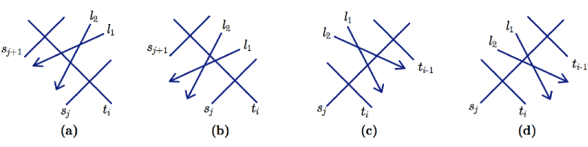
Figure 5: An intersection is moved (from (a) to (b) and from (c) to (d)) across an edge in the grid. Note that the intersection moved is of two paths whose directions indicate their slopes, whereas in the grid the slope is drawn.

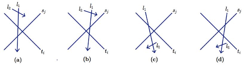
Figure 6: A non-rightmost path $l_{1}$ is moved across an intersection in the grid (from (a) to (b) and from (c) to (d)). The diagram does not indicate where the path $l_{2}$ is; only where $l_{1}\cap l_{2}$ is relative to the intersection $t_{i}\cap s_{j}$.

Step 2. Moving a non-rightmost path across an intersection.

In this paragraph we discuss the case shown in Fig. 6. The path $l_{1}$ is non-rightmost because there is another path $l_{2}$ to the right of it. If $l_{1}$ and $l_{2}$ have the same slope, then the capacity does not change no matter how $l_{1}$ moves on the left of $l_{2}$ according to the discussion in Proposition 15. When they intersect, there are two cases: from (a) to (b), $l_{1}$ crosses an intersection when after its intersection with $l_{2}$; from (c) to (d), $l_{1}$ crosses an intersection before its intersection with $l_{2}$. Only the labels listed in the table below are changed.

(a) to (b)	Change	Reason	(c) to (d)	Change	Reason
$t_{i}\cap s_{j}$	$+1$	It cannot reach $l_{1}$ in (a)	$t_{i}\cap s_{j}$	0	It reaches $l_{1}$ via $l_{2}$ in (c)
$l_{1}\cap t_{i}$	$-1$	It cannot reach $s_{j}$ in (b)	$l_{1}\cap t_{i}$	$-1$	It cannot reach $s_{j}$ in (d)
$l_{1}\cap s_{j}$	0	It reaches $t_{i}$ via $l_{1}$ in (b)	$l_{1}\cap s_{j}$	0	It reaches $t_{i}$ via $l_{1}$ in (d)

Therefore, a non-rightmost path can be moved freely across an intersection if it has already intersected with a path on its right. Before the intersection with that path, it should move farther from the rightmost intersection in order to increase the capacity. How a rightmost path should move across intersections in the grid or exit the grid has been discussed in Proposition 15.

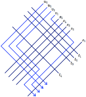
Figure 7: The best arrangement for Case One, where $a=5$, $b=4$, and $c=d=2$.

Now our tools are enough to deal with Case One. All the paths (with slopes $k_{3}$ and $k_{4}$ form another grid. It has also a rightmost corner, and we call the intersection of the leftmost lines with slopes $k_{3}$ and $k_{4}$ the bottom corner. We can first move the bottom corner to between $s_{1}$ and $s_{2}$ of the $k_{1}$-$k_{2}$ grid using our transformations above that do not reduce the capacity. This is possible because we can move together the parts of the two paths that are after their intersection, and then move the intersection along the route. Then we repeat the operation for the corner closest to the bottom corner, and so on, until all intersections of the paths are to the left of $s_{1}\cap t_{b}$, and between $s_{1}$ and $s_{2}$. After that, the paths can be moved in the grid without considering the intersections between the paths using our transformations that do not reduce the capacity to their locations shown in Fig. 7.

The number of deliveries in Fig. 7 is

$$\sum_{k=2}^{b+c+d+1}k+c\sum_{k=b+c+2}^{b+c+d+1}k+b\sum_{k=b+c+2}^{a+b+c+1}+$$

$$d\sum_{k=b+c+2}^{a+b+c}k+(a-1)\sum_{k=1}^{d}k+c\sum_{k=b+c+d+2}^{a+b+c+d}k+b\sum_{k=a+b+c+2}^{a+b+c+d}k+bc(a+b+c+d).$$

Case Two

In this case, $k_{3}$ and $k_{4}$ have different signs. All lines (shown as paths in the diagrams) of slopes $k_{3}$ and $k_{4}$ form another grid. The lines $l,l^{\prime}$ on which the rightmost intersection of this $k_{3}$-$k_{4}$ grid lies on divide the plane into four regions. We will call the region to the left of both $l$ and $l^{\prime}$ the Region I, that between the two lines the Region II, and that to the right of both lines the Region III. We also define that the part of $l\cup l^{\prime}$ that can reach both lines is in Region I, and the part of $l\cup l^{\prime}$ that can reach only one of $l$ and $l^{\prime}$ is in the Region II. Fig. 8 shows the regions. Depending on the arrangement, the intersections in the $k_{1}$-$k_{2}$ grid might belong to any of the three regions (except the rightmost one, which must be in Region III); however, any intersection cannot reach an intersection in another region with smaller index, otherwise one of $l$ and $l^{\prime}$ would intersect some line with slope $k_{1}$ or $k_{2}$ more than once.

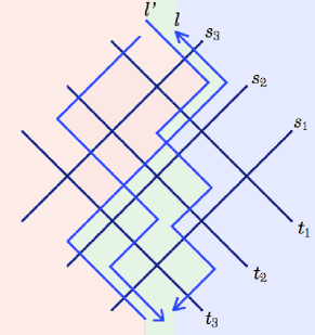
Figure 8: In this arrangement, Region I is painted red, Region II is painted green, and Region III is blue. The lines should be included in the regions, but to be visible, they are not painted.

Because $k_{3}k_{4}<0$, the intersection $l\cap l^{\prime}$ can reach any line with slope $k_{1}$ or $k_{2}$, and so does any intersection in Region I. The number of lines that an intersection in Region I can reach is then $n$ minus the number of lines in the $k_{3}$-$k_{4}$ grid that the intersection cannot reach. This is a fixed number for any intersection in the $k_{3}$-$k_{4}$ grid in the Region I, and at most $n$ for other intersections. It is clear that by moving paths across intersections in the $k_{1}$-$k_{2}$ grid, we can produce an arrangement with no less capacity where any intersection in the $k_{1}$-$k_{2}$ grid in Region I can reach all lines with slopes $k_{3}$ and $k_{4}$.

Step 1. Moving all lines with slopes $k_{3}$ and $k_{4}$ together.

We have the following two operations: (i) move an intersection in the $k_{3}$-$k_{4}$ grid across an edge in the $k_{1}$-$k_{2}$ grid (Fig. 9); (ii) move a line in the $k_{3}$-$k_{4}$ grid across an intersection in the $k_{1}$-$k_{2}$ grid (Fig. 10).

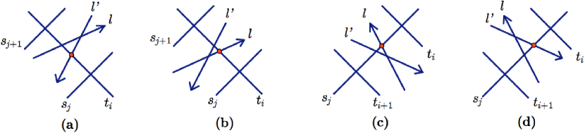
Figure 9: From (a) to (b), the rightmost intersection $l\cap l^{\prime}$ in the $k_{3}$-$k_{4}$ grid is moved below $t_{i}$; from (c) to (d) it is moved above $s_{j}$. Only the number of lines the marked point can reach changes.

Because $l\cap l^{\prime}$ is the rightmost intersection in the $k_{3}$-$k_{4}$ grid, there cannot be any intersections in this grid in Region II. So we need only discuss operation (i) on $l\cap l^{\prime}$ (Fig. 9), which is the only intersection on the boundary between Regions II and III. (The discussion on the boundary between Regions I and II is similar, except that the same number of lines in the $k_{3}$-$k_{4}$ grid can be reached in each arrangement, which do not change the result). In the diagrams, only the number of lines the red intersection can reach may change because the other two intersections involved in the change are both on either $l$ or $l^{\prime}$, and we know that each of them can reach all lines in the $k_{1}$-$k_{2}$ grid and only the lines $l$ and $l^{\prime}$ in the $k_{3}$-$k_{4}$ grid. The lines that the red point can reach are listed in the table below.

Fig. 9	Lines it can reach	Number	Fig. 9	Lines it can reach	Number
(a)	$t_{1},\ldots,t_{b},s_{1},\ldots,s_{j},l^{\prime}$	$b+j+1$	(b)	$t_{1},\ldots,t_{i},s_{1},\ldots,s_{a},l$	$a+i+1$
(c)	$t_{1},\ldots,t_{i},s_{1},\ldots,s_{a},l$	$a+i+1$	(d)	$t_{1},\ldots,t_{b},s_{1},\ldots,s_{j},l^{\prime}$	$b+j+1$

Therefore, the intersection $l\cap l^{\prime}$ can be moved either above $t_{i}$ or below $s_{j}$. Because moving from Fig. 9(b) to Fig. 9(a) changes the number of deliveries by $(j-i)+(b-a)$, and moving from Fig. 9(d) to Fig. 9(c) changes the number of deliveries by $(i-j)+(a-b)$, one of the changes must be nonnegative (as they sum to zero). And this movement makes the capacity no less.

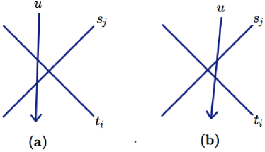
Figure 10: The line $u$ of slope $k_{3}$ or $k_{4}$ is moved across an intersection $s_{j}\cap t_{i}$. We assume that $u\neq l$ and $u\neq l^{\prime}$.

Operation (ii) is simpler (Fig. 10). On the boundary between Region I and II, it always increases the capacity because one intersection in Region II is moved into Region I, and intersections initially in Region I still remain in Region I. At other locations (Regions II and III), only the lines in the $k_{3}$-$k_{4}$ grid whose directions are away from $l\cap l^{\prime}$ can occur, so the discussion is essentially the same as Case One, which we omit. Now, we notice that every operation (i) can be immediately followed by an operation (ii) that puts one more intersection in the $k_{1}$-$k_{2}$ grid in a region with smaller index. Therefore, after a series of operations, the arrangement is transformed to an arrangement with no less capacity such that there are no intersections in the $k_{1}$-$k_{2}$ grid between lines in the $k_{3}$-$k_{4}$ grid. Note that in this step we do not alter where $l$ and $l^{\prime}$ leave the $k_{1}$-$k_{2}$ grid; it will be discussed in Step 3.

Step 2. Moving the intersections.

In this step, only operation (i) is needed to move the intersections in the $k_{3}$-$k_{4}$ grid. From right to left, we label the lines with slope $k_{3}$ by $u_{1},u_{2},\ldots,u_{c}$ and the lines with slope $k_{4}$ by $v_{1},v_{2},\ldots,v_{d}$. Suppose we want to move the intersection $u_{k}\cap v_{l}$ across either a $t_{i}$ (from Fig. 11(a) to Fig. 11(b)) or a $s_{j}$ (from Fig. 11(c) to Fig. 11(d)). Only the red point in the diagrams needs discussion because the other two points involved in the movement can directly reach $u_{k}\cap v_{l}$, and reach from that all lines in the $k_{1}$-$k_{2}$ grid. And clearly the movement cannot change the number of lines these points can reach in the $k_{3}$-$k_{4}$ grid. We have several cases.
Case i. $k\neq 1$ and $l\neq 1$. The red point can always reach an intersection in the $k_{3}$-$k_{4}$ grid and thus all lines in the $k_{1}$-$k_{2}$ grid. So the capacity does not change.
Case ii. $k=1$ and $l\neq 1$. Moving from (a) to (b) and from (c) to (d) always results in an arrangement with no less capacity because the red points in (b) and (d) can reach $u_{k}\cap l_{1}$, and thus all lines in the $k_{1}$-$k_{2}$ grid.
Case iii. $k\neq 1$ and $l=1$. This case is symmetric to Case ii, so similarly moving from (b) to (a) and from (d) to (c) always results in an arrangement with no less capacity.
Case iv. $k=l=1$. This case has already been discussed in Case One.

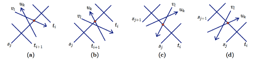
Figure 11: From (a) to (b), the intersection $u_{k}\cap v_{l}$ in the $k_{3}$-$k_{4}$ grid is moved below $s_{j}$; from (c) to (d) it is moved below $t_{i}$. Only the number of lines the marked point can reach changes. Here the index $l$ is not related to the rightmost line $l$ mentioned before.

It is not hard to see that the operations above that result in no less capacity can move all intersections in the $k_{3}$-$k_{4}$ grid outside the $k_{1}$-$k_{2}$ grid, transforming the arrangement to the form in Fig. 12 (where the enclosed region in (a) should be topologically equivalent (for the locations of the lines) to the enclosed region in (b), and the red, black, and light blue lines are only for the description and are not in the RGMSN).

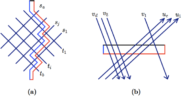
Figure 12: An arrangement can be obtained if the enclosed region in (b) is embedded as the enclosed region in (a). In this diagram, $a=b=d=4$, $c=i=3$, and $j=2$.

Step 3. Where $l$ and $l^{\prime}$ leave the $k_{1}$-$k_{2}$ grid.

Suppose lines $l$ and $l^{\prime}$ intersect $s_{1}$ between $t_{i}$ and $t_{i+1}$, and intersect $t_{1}$ between $s_{j}$ and $s_{j+1}$. We directly compute the total number of deliveries.

Intersections	Total deliveries
$s_{1}\cap t_{1},\ldots,s_{1}\cap t_{i},s_{2}\cap t_{1},\ldots,s_{j}\cap t_{1}$	$\sum_{k=2}^{i+1}k+\sum_{k=3}^{j+1}k$
$v_{1}\cap s_{k},v_{1}\cap t_{k}$	$\sum_{k=2}^{b-i+1}k+(b+2)i+\sum_{k=b+3}^{b+j+1}k+(b+j+1)+\sum_{k=b+j+2}^{a+b+1}k$
$v_{1}\cap u_{k}$	$\sum_{k=a+b+2}^{a+b+c+1}k$
$u_{k}\cap s_{l},u_{k}\cap t_{l}$	$(a+b)\sum_{k=a+b+2}^{a+b+c+1}k$
$u_{k}\cap v_{2},\ldots,u_{k}\cap v_{d}$	$(d-1)\sum_{k=a+b+2}^{a+b+c+1}k+c\sum_{k=1}^{d-1}k$
$v_{k}\cap s_{l},v_{k}\cap t_{l}$	$(a+b)\sum_{k=a+b+c+2}^{a+b+c+d}k$
Other $s_{k}\cap t_{l}$	$(a+b+c+d)(ab-i-j+1)$

In the formula for the total number of deliveries, the terms depending on $i$ and $j$ are

$$2(i^{2}-(n-2)i)+(j^{2}-(2n-5)j).$$

When this is maximized, we must have $i=j=1$ due to the range of $i$ and $j$. However, even when $i=j=1$, the formula is smaller than that in Case One by $2(n-3)>0$ when expanded, so Case One gives the maximum capacity, which is the maximum of

$$\frac{a+d+2(b+c)+1}{2n}+\frac{ad+bc(a+d-1)+(b+c)-(b+c)^{2}}{2n(ad+bc+(a+d)(b+c))}.$$

To maximize this, we observe that for given $a+d$ and $b+c$, $ad$ must be minimized while $bc$ must be maximized, so we have $d=1$ and $|b-c|\leq 1$. In this case basic calculus methods (omitted) show that the capacity is decreasing with $a$ increasing, so $a=1$ or $a=2$. If we split into two cases according to the parity of $n$, in each case we need only compare two numbers, and we found that in each case one number is always larger than the other. The larger number is thus the maximum capacity, which is

$$\begin{cases}\displaystyle\frac{n^{3}+2n^{2}-2n-4}{n(n^{2}+4n-8)},&n\text{ is odd},\\ \displaystyle\frac{n^{3}+2n^{2}-3n-4}{n(n^{2}+4n-9)},&n\text{ is even}.\end{cases}$$

∎

Unfortunately, the casework method above can only give the exact maximum capacity for at most four slopes. For five or more slopes, it fails.

Question 19.

What is the maximum capacity of an RGMSN of $n$ sensors with only $s$ slopes allowed ($s\geq 5$)?

Now we compute the expected capacity of a random RGMSN with at most four slopes. The method is the same as Theorem 17, except that the integrals are different. In general, suppose the $s$ slopes that are chosen independently and uniformly from $[0,1]$ are $a_{1}<a_{2}<\cdots<a_{s}$, and there are $n_{k}$ lines with slope $a_{k}$ for each $k$. Let $u$ be a line $y=a_{i}x+b_{i}$, $v$ be a line $y=a_{j}x+b_{j}$, and $w$ be a line $y=a_{k}x+b_{k}$, where $1\leq i<j\leq s$. If $k\leq i$ or $k\geq j$, the probability that $u\cap v$ can reach $w$ in one hop is

$$\frac{\displaystyle\int_{0}^{1}\int_{a_{1}}^{1}\int_{a_{2}}^{1}\cdots\int_{a_{s}}^{1}\int_{0}^{1}\int_{0}^{1}\min\bigg{\{}1,\max\bigg{\{}0,b_{j}+(b_{k}-b_{j})\frac{a_{j}-a_{i}}{a_{j}-a_{k}}\bigg{\}}\bigg{\}}\,\mathrm{d}b_{k}\,\mathrm{d}b_{j}\,\mathrm{d}a_{s}\ldots\,\mathrm{d}a_{2}\,\mathrm{d}a_{1}}{\displaystyle\int_{0}^{1}\int_{a_{1}}^{1}\int_{a_{2}}^{1}\cdots\int_{a_{s}}^{1}\,\mathrm{d}a_{s}\ldots\,\mathrm{d}a_{2}\,\mathrm{d}a_{1}}=\frac{1}{2}.$$

If $i<k<j$, then $u\cap v$ can reach $w$ in one hop. If $k\leq i$, the probability that $u\cap v$ can reach the leftmost line with slope $a_{l}$ where $l<k$ is

$$\frac{\displaystyle\begin{multlined}\displaystyle\int_{0}^{1}\int_{a_{1}}^{1}\int_{a_{2}}^{1}\cdots\int_{a_{s}}^{1}\int_{0}^{1}\int_{0}^{1}\cdots\int_{0}^{1}\min\bigg{\{}1,\max\bigg{\{}0,\max_{1\leq l<k}\bigg{\{}b_{j}+(b_{l}-b_{j})\frac{a_{j}-a_{i}}{a_{j}-a_{l}}\bigg{\}}\bigg{\}}\bigg{\}}\\ \,\mathrm{d}b_{1}^{n_{1}}\ldots\,\mathrm{d}b_{k-1}^{n_{k-1}}\,\mathrm{d}b_{j}\,\mathrm{d}a_{s}\ldots\,\mathrm{d}a_{2}\,\mathrm{d}a_{1}\end{multlined}\displaystyle\int_{0}^{1}\int_{a_{1}}^{1}\int_{a_{2}}^{1}\cdots\int_{a_{s}}^{1}\int_{0}^{1}\int_{0}^{1}\cdots\int_{0}^{1}\min\bigg{\{}1,\max\bigg{\{}0,\max_{1\leq l<k}\bigg{\{}b_{j}+(b_{l}-b_{j})\frac{a_{j}-a_{i}}{a_{j}-a_{l}}\bigg{\}}\bigg{\}}\bigg{\}}\\ \,\mathrm{d}b_{1}^{n_{1}}\ldots\,\mathrm{d}b_{k-1}^{n_{k-1}}\,\mathrm{d}b_{j}\,\mathrm{d}a_{s}\ldots\,\mathrm{d}a_{2}\,\mathrm{d}a_{1}}{\displaystyle\int_{0}^{1}\int_{a_{1}}^{1}\int_{a_{2}}^{1}\cdots\int_{a_{s}}^{1}\int_{0}^{1}\cdots\int_{0}^{1}\,\mathrm{d}b_{1}^{n_{1}}\ldots\,\mathrm{d}b_{k-1}^{n_{k-1}}\,\mathrm{d}a_{s}\ldots\,\mathrm{d}a_{2}\,\mathrm{d}a_{1}}.$$

This integral when $s=4$ and $n\to\infty$ equals $3/4$, $5/6$, $2/3$, and $3/4$ for $(i,j,k)=(2,3,2)$, $(2,4,2)$, $(3,4,2)$, and $(3,4,3)$ respectively. If $k\geq j$, the probability that $u\cap v$ can reach the rightmost line with slope $a_{l}$ where $l>k$ is

$$\frac{\displaystyle\begin{multlined}\displaystyle\int_{0}^{1}\int_{a_{1}}^{1}\int_{a_{2}}^{1}\cdots\int_{a_{s}}^{1}\int_{0}^{1}\int_{1}^{0}\cdots\int_{1}^{0}\min\bigg{\{}1,\max\bigg{\{}0,\max_{k<l\leq s}\bigg{\{}b_{j}+(b_{l}-b_{j})\frac{a_{j}-a_{i}}{a_{j}-a_{l}}\bigg{\}}\bigg{\}}\bigg{\}}\\ \,\mathrm{d}(1-b_{k+1})^{n_{k+1}}\ldots\,\mathrm{d}(1-b_{s})^{n_{s}}\,\mathrm{d}b_{j}\,\mathrm{d}a_{s}\ldots\,\mathrm{d}a_{2}\,\mathrm{d}a_{1}\end{multlined}\displaystyle\int_{0}^{1}\int_{a_{1}}^{1}\int_{a_{2}}^{1}\cdots\int_{a_{s}}^{1}\int_{0}^{1}\int_{1}^{0}\cdots\int_{1}^{0}\min\bigg{\{}1,\max\bigg{\{}0,\max_{k<l\leq s}\bigg{\{}b_{j}+(b_{l}-b_{j})\frac{a_{j}-a_{i}}{a_{j}-a_{l}}\bigg{\}}\bigg{\}}\bigg{\}}\\ \,\mathrm{d}(1-b_{k+1})^{n_{k+1}}\ldots\,\mathrm{d}(1-b_{s})^{n_{s}}\,\mathrm{d}b_{j}\,\mathrm{d}a_{s}\ldots\,\mathrm{d}a_{2}\,\mathrm{d}a_{1}}{\displaystyle\int_{0}^{1}\int_{a_{1}}^{1}\int_{a_{2}}^{1}\cdots\int_{a_{s}}^{1}\int_{1}^{0}\cdots\int_{1}^{0}\,\mathrm{d}(1-b_{k+1})^{n_{k+1}}\ldots\,\mathrm{d}(1-b_{s})^{n_{s}}\,\mathrm{d}a_{s}\ldots\,\mathrm{d}a_{2}\,\mathrm{d}a_{1}}.$$

This integral when $s=4$ and $n\to\infty$ equals $3/4$, $2/3$, $5/6$, and $3/4$ for $(i,j,k)=(1,2,2)$, $(1,2,3)$, $(1,3,3)$, and $(2,3,3)$ respectively.

Let $P(i,j,k)$ be the probability, when $n\to\infty$, that the intersection of a line with slope $a_{i}$ and a line with slope $a_{j}$ can reach a line with slope $a_{j}$, then we have the following.

$i$	$j$	$k$	$P(i,j,k)$	$i$	$j$	$k$	$P(i,j,k)$	$i$	$j$	$k$	$P(i,j,k)$	$i$	$j$	$k$	$P(i,j,k)$
1	2	1	$1/2$	1	2	2	$7/8$	1	2	3	$5/6$	1	2	4	$1/2$
1	3	1	$1/2$	1	3	2	1	1	3	3	$11/12$	1	3	4	$1/2$
1	4	1	$1/2$	1	4	2	1	1	4	3	1	1	4	4	$1/2$
2	3	1	$1/2$	2	3	2	$7/8$	2	3	3	$7/8$	2	3	4	$1/2$
2	4	1	$1/2$	2	4	2	$11/12$	2	4	3	1	2	4	4	$1/2$
3	4	1	$1/2$	3	4	2	$5/6$	3	4	3	$7/8$	3	4	4	$1/2$

Therefore, the expected capacity for an RGMSN with $s=4$ slopes is the average of the 24 numbers in the table above, which is $17/24$.

Proposition 20 (Expectation for Four-Slope RGMSN).

The expected capacity for an RGMSN with $n$ sensors and at most four slopes is $17/24$.

The main difficulty of generalizing this to any number of slopes is the integrals above, which are out of reach of our computational power when $s$ is aribitrary.

Complexity of Deciding Realizability of (R)CMSNs as (R)GMSNs

Although many RCMSNs can be generated from a geometric construction (GMSN), most cannot. Knuth proved in [4] that the number of GMSNs of $n$ sensors is less than $3^{\binom{n+1}{2}}$, but clearly the number of RCMSNs of $n$ sensors is $\binom{n}{2}!$. Therefore, we propose the following question: which RCMSNs are GMSNs? Now we show that there is unlikely an efficient algorithm:

Theorem 21 (GMSN Realizability Problem).

Given an RCMSN, deciding whether it is generated from a GMSN is NP-Hard.

(Note: below, a pseudoline means a simple curve that is not closed; and we do not allow two pseudolines, or one pseudoline and one line, to intersect more than once.)

Proof.

Shor [3] showed that deciding the stretchability of a pseudoline arrangement is NP-Hard. Because all pseudoline arrangements in his paper contain only pseudolines that intersect any additional vertical line at most once, we shall consider only such pseudolines. We also assume that any additional vertical line contains at most one intersection of the pseudolines. Because of this, it is possible to draw two vertical lines such that all intersections of the pseudolines fall between them, and each pseudoline “starts” (at infinity) on the left of the two vertical lines and “ends” on the right of the two vertical lines.

Suppose the arrangement contains $n$ pseudolines, each two of them intersect exactly once between the two vertical lines. We convert this arrangement to a finite sequence of numbers as follows. Let all the intersections ordered by their $x$-coordinate be $p_{1}$, …, $p_{\binom{n}{2}}$. For each $1\leq k\leq\binom{n}{2}$, we draw a vertical ray upward from $p_{k}$ and let $a_{k}$ be the total number of intersections this ray form with all the pseudolines. Then $a_{k}\in\{1,\ldots,n-1\}$, and we have a sequence $\{a_{k}\}_{k=1}^{n(n-1)/2}$.

Let $\sigma$ be any permutation of $\{1,\ldots,n\}$. We can convert the sequence $\{a_{k}\}$ to an RCMSN using the following algorithm:

1 $\tau\leftarrow\sigma$
2 for $k$ from 1 to $\binom{n}{2}$
3    $c_{k}\leftarrow\{\tau(a_{k}),\tau(a_{k}+1)\}$
4    swap $\{\tau(a_{k}),\tau(a_{k}+1)\}$
5 return $\{c_{k}\}_{k=1}^{n(n-1)/2}$

Here $\sigma$ is the labels of the pseudolines at the vertical line on the left of all intersections (ordered by their $y$-coordinates), and $\tau$ stores the current labels of the pseudolines at an additional vertical line immediately before and after each intersection, such that the labels are consistent with $\sigma$ (guaranteed by line 4). Now, the geometric realizabilities of all $n!$ RCMSNs that can be generated from the pseudoline arrangement are equivalent by a relabeling of lines using $\sigma$. Therefore, we need to prove that the pseudoline arrangement (if exists) is uniquely determined from an RCMSN up to a relabeling of lines and isomorphism (two arrangements are isomorphic if the graphs, where the vertices are the regions in the arrangement and the edges are adjacency of regions, are isomorphic).

The following algorithm converts an RCMSN $\{c_{k}=\{x_{k},y_{k}\}\}_{k=1}^{n(n-1)/2}$ (where each $x_{k},y_{k}\in\{1,\ldots,n\}$) into a sequence $\{a_{k}\}_{k=1}^{n(n-1)/2}$ (where each $a_{k}\in\{1,\ldots,n-1\}$) as described before, and also reports some clearly nonrealizable RCMSNs:

1 $\tau\leftarrow\text{identity}\in S_{n}$
2 $T\leftarrow\text{linked list of }\{1,\ldots,n\}\text{ with no links}$
3 for $k$ from 1 to $\binom{n}{2}$
4    if $T\text{.degree}(\tau(x_{k}))=2$ or $T\text{.degree}(\tau(y_{k}))=2$
5      return non-realizable
6    else if not $T$.linked$(\tau(x_{k}),\tau(y_{k}))$
7      $T$.link$(\tau(x_{k}),\tau(y_{k}))$
8      swap $\{\tau(x_{k}),\tau(y_{k})\}$
9  $\sigma(1)\leftarrow T$.head
10 for $k$ from 2 to $n$
11    $\sigma(k)\leftarrow T$.next$(\sigma(k-1))$
12 $\tau\leftarrow\sigma$
13 for $k$ from 1 to $\binom{n}{2}$
14    if $|\tau^{-1}(x_{k})-\tau^{-1}(y_{k})|\neq 1$
15      return non-realizable
16    else
17      $a_{k}\leftarrow\min\{\tau^{-1}(x_{k}),\tau^{-1}(y_{k})\}$
18      swap $\{\tau^{-1}(x_{k}),\tau^{-1}(y_{k})\}$
19 return $\sigma$ and $\{a_{k}\}_{k=1}^{n(n-1)/2}$

In lines 1–8 we first determine which two numbers in the given RCMSN might represent adjacent pseudolines on the left of both vertical lines we inserted in a GMSN. $T$ is a list of consecutive lines, and $\tau$ represents that “the current $k$th pseudoline from the top is the $\tau(k)$-th pseudoline on the left of both vertical lines we inserted.” Only adjacent pseudolines are allowed to intersect because otherwise the pseudolines between them cannot extend across the intersection. Thus, if we fail to build a whole list $T$, no such GMSN exists. On the other hand, if the list $T$ is built, it represents the relabeling of lines discussed in the previous algorithm and is thus stored in $\sigma$ (lines 9–11). In lines 12–18, the meaning of $\tau$ is the same as that in the previous algorithm, and we reverse the previous algorithm to find $\{a_{k}\}$. If we fail to reverse it, then at some point there must be two nonadjacent lines that are required to intersect, so clearly no such GMSN exists.

From this algorithm, we see that if an RCMSN is geometrically realizable, it corresponds to at most two pairs $(\sigma,\{a_{k}\})$ (because $T$ can be read from both sides), and their corresponding pseudoline arrangements are isomorphic as they are mirror images of each other. We shall ignore $\sigma$ because it does not change the pseudoline arrangement.

Now we need to prove that every sequence $\{a_{k}\}_{k=1}^{n(n-1)/2}$ where $a_{k}\in\{1,\ldots,n-1\}$ describes at most one pseudoline arrangement. First, it describes one arrangement naturally: Consider all points $(k,j)$ where $0\leq k\leq\binom{n}{2}$ and $1\leq j\leq n$ are integers. We draw a ray from each $(0,j)$ horizontally to the left and from each $(\binom{n}{2},j)$ horizontally to the right. Then, for each $k$ we connect $(k-1,a_{k})$ to $(k,a_{k}+1)$ by a segment, $(k-1,a_{k}+1)$ to $(k,a_{k})$ by a segment, and $(k-1,j)$ to $(k,j)$ by a segment for all $j\not\in\{a_{k},a_{k}+1\}$. If this is not a pseudoline arrangement, then two curves must have intersected twice, and the RCMSN corresponds to no pseudoline arrangement. Otherwise, the RCMSN is generated by at least one pseudoline arrangement.

Given a pseudoline arrangement whose sequence is $\{a_{k}\}$, we need to prove that it is isomorphic to the pseudoline arrangement above. We give a region color 1 if it is adjacent to the region above all pseudolines. Then we give a region color $r$ if it is adjacent to an already colored region with color $r-1$. By definition, the number of regions with color $r$ is equal to the number of $r$’s in $\{a_{k}\}$. So in our two arrangements the number of regions with each color is equal. Also, it is clear that in both arrangements, the leftmost and rightmost regions with color $r$ must be adjacent to the leftmost and rightmost regions with color $r\pm 1$, respectively. If a region immediately on the left of intersection $p_{j}$ and a region immediately on the right of intersection $p_{k}$ have colors differing by one (which is the only case they might be adjacent, by definition), then they are adjacent if and only if $k<j$ because the pseudoline connecting the two intersections is either a shared edge or an edge that separates the two regions. There are no other possible cases of adjacent regions, so the graph of adjacent regions is determined by the sequences $\{a_{k}\}$. Therefore the two pseudoline arrangements we have are isomorphic.

Hence, if we have an algorithm for the geometric realizability of RCMSNs, then for every pseudoline arrangement we can convert it to an RCMSN in polynomial time and determine if it is generated from a GMSN; and the GMSN as a pseudoline arrangement must be isomorphic to the given one because they correspond to the same RCMSN, as discussed above. ∎

Although it is hard to determine if an RCMSN is generated from a GMSN, we may consider the similar problem of determining if a CMSN is generated from an RGMSN with limited number of slopes. For example, this problem is easy when the RGMSN has only one or two slopes, because the only possible shape of the network is a grid in this case. It turns out that for three or more slopes we can also solve this problem in polynomial time, as shown in the theorem below. We reduce the problem into linear programming and the same problems with a smaller number of slopes. However, our algorithm has complexity that is exponential on the number of slopes.

Theorem 22 (RGMSN Realizability Problem).

For any fixed positive integer $s$, there is an algorithm with polynomial complexity with respect to the number of sensors for deciding whether a given CMSN is generated from an RGMSN with at most $s$ slopes.

Proof.

First, we use the method in Theorem 21 to convert a CMSN into a pseudoline arrangement when possible. If this is not possible, then the CMSN is clearly not realizable. Now we construct a graph where the vertices represent the pseudolines, and two vertices are connected by an edge if the two pseudolines do not intersect. If any component in this graph is not a complete graph, then the pseudoline arrangement is clearly not stretchable since being parallel is transitive. If this graph has more than $s$ connected components, then the CMSN is also not realizable with at most $s$ slopes because we can find four pairwise intersecting pseudolines. If this graph has less than three connected components, then the CMSN is clearly realizable as a grid.

Base Case: $s=3$.

We assume that the graph has three connected components $A$, $B$, and $C$. Also, we assume that all pseudolines in the arrangement we get are monotone, meaning that each pseudoline intersects any vertical line or horizontal line exactly once. We can easily modify Theorem 21’s method so that it always gives monotone pseudolines. Now we label the pseudolines in $A$ as $a_{1}$, $a_{2}$, … in their order from top to bottom when intersecting with a vertical line, and label the pseudolines in $B$ as $b_{1}$, $b_{2}$, … similarly, but from bottom to top. Note that the direction “top to bottom” is arbitrary; it can be reversed. We assume that $\min\{|A|,|B|,|C|\}\geq 2$ since otherwise the arrangement is clearly stretchable. Also, for a horizontal line above all intersections in the arrangment, we assume without loss of generality that its leftmost intersection with the arrangment is with a line in $B$, and its rightmost intersection with the arrangement is with a line in $A$. These are merely relabeling of pseudolines.

Our strategy is to suppose the arrangement is stretchable and try to construct it unless we find a contradiction. For an arrangement stretchable with at most three slopes, we first apply an affine transformation (which does not change the arrangement) to make all lines in $A$ have slope $-1$ and all lines in $B$ have slope 1. Now we try to make all lines in $C$ vertical. We use the following procedure (Fig. 13):

1 $(A^{\prime},B^{\prime})\leftarrow(A,B)$
2 $(l_{A},r_{A},l_{B},r_{B})\leftarrow(a_{1},a_{|A|},b_{1},b_{|B|})$
3 repeat
4    $(s_{A},s_{B})\leftarrow(|A^{\prime}|,|B^{\prime}|)$
5    for each $a\in A^{\prime}$
6      for each $c\in C$
7        if $a\cap c$ is between $l_{B}$ and $r_{B}$
8          $B^{\prime}\leftarrow B^{\prime}\cup(\text{the line through $a\cap c$ with slope 1})$
9    for each $b\in B^{\prime}$
10      for each $c\in C$
11        if $b\cap c$ is between $l_{A}$ and $r_{A}$
12          $A^{\prime}\leftarrow A^{\prime}\cup(\text{the line through $b\cap c$ with slope $-1$})$
13 until $s_{A}=|A^{\prime}|$ and $s_{B}=|B^{\prime}|$

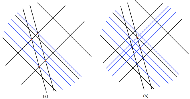
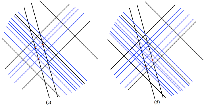
Figure 13: An example of the procedure. All additional lines are blue, and the intersections where additional lines are added are marked. (a) The arrangement at line 9 of the first cycle. (b) The arrangement at line 13 of the first cycle. (c) The arrangement at line 9 of the second cycle. (d) The arrangement at the end.

If this procedure terminates, then we can adjust the distances between the lines so that each cell in the grid formed by $A^{\prime}$ and $B^{\prime}$ is a square. Then, because there are no additional lines in satisfying the conditions in line 9 and line 13 in the algorithm, all intersections of lines in $C$ and the grid are at intersections of gridlines; lines satisfying this condition can only be vertical.

Therefore we need to move the lines by some small distances before the procedure above such that the procedure would terminate. This is not difficult: we move all lines by sufficiently small distances such that they have rational intercepts; then we rotate all lines in $C$ by a sufficiently small angle such that the angle between each line in $C$ and each line in $A$ is the arctangent of a rational number. After these operations, there are only finitely many lines that could possibly be generated in the procedure above, so the procedure must terminate.

Now we suppose that all lines in $A$ have slope $-1$, all lines in $B$ have slope 1, and all lines in $C$ are vertical. Let $x_{k}$ be the distance between lines $a_{k}$ and $a_{k+1}$, and $y_{k}$ be the distance between lines $b_{k}$ and $b_{k+1}$. Consider the intersection $a_{i}\cap b_{l}$ and $a_{j}\cap b_{k}$, where $i<j$ and $k<l$. (In any other order of $i$, $j$, $k$, and $l$, the order of the two intersections’ $x$-coordinates is determined.) If there is a pseudoline in $C$ intersecting both ray $(a_{i}\cap b_{l})(a_{i}\cap b_{l+1})$ and ray $(a_{j}\cap b_{k})(a_{j}\cap b_{k-1})$ (Fig. 14), then in the stretched arrangement $a_{i}\cap b_{l}$ has a smaller $x$-coordinate than $a_{j}\cap b_{k}$, and we have $\sum_{t=i}^{j-1}x_{t}>\sum_{t=k}^{l-1}y_{t}$; if there is a pseudoline in $C$ intersecting both ray $(a_{i}\cap b_{l})(a_{i}\cap b_{l-1})$ and ray $(a_{j}\cap b_{k})(a_{j}\cap b_{k+1})$, then in the stretched arrangement $a_{i}\cap b_{l}$ has a larger $x$-coordinate than $a_{j}\cap b_{k}$, and we have $\sum_{t=i}^{j-1}x_{t}<\sum_{t=k}^{l-1}y_{t}$. This is a linear programming problem, and we can determine its consistency in polynomial time. (Note: although we have strict inequalities here, we can scale the arrangement to convert any $p<q$ to the equivalent $p+1\leq q$.) If it is consistent, then the arrangement of lines with distances $\{x_{k}\}$ and $\{y_{k}\}$ and lines in $C$ in appropriate places gives the GMSN when rotated a small angle. If it is inconsistent, then the pseudoline arrangement is not stretchable because we have found a contradiction.

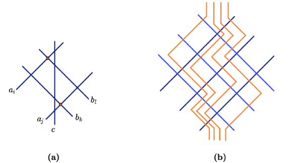
Figure 14: (a) The line $c\in C$ gives a constraint on the distances between lines. (b) An example of a nonstretchable pseudoline arrangement.

Second Base Case: $s=4$.

From the $s=3$ case, we see that every RGMSN with four slopes can be transformed into one with the four slopes equal to 0, 1, $\infty$, and another number $k<0$ (hereby that will be called a RGMSN_k). So our question is that, given a CMSN, whether there exists $k$ such that the network can be realized as an RGMSN_k. Because we may reflect the whole network over the line $x+y=0$, without loss of generality, the range of $k$ can be further limited to $0<-k<1$.

If we know the number $k$, we can decide in polynomial time whether the CMSN is realizable as a RGMSN_k using the inequalities that describe the order of intersections of one line and other lines on the line. This is a linear programming problem. For the problem with $k$ unknown, our algorithm is to find $O(n^{4})$ different potential values of $k$ (if there are $n$ sensors in the CMSN), and show that if the given CMSN is realizable, it can be realized with one of those specific $k$ values. (The potential values of $k$ depend on the CMSN given.) So we run linear programming at most $O(n^{4})$ times to find out the realizability.

Now suppose $k$ is unknown. Then we have a system of strict inequalities that become linear if $k$ is regarded as constant, and all inequalities are linear for $k$. The set of values of $k$ such that the linear program is feasible must be an open set because all inequalities are strict. Let $-k_{0}$ be the infimum of that set, then it is a boundary point. Clearly, with $k=k_{0}$ the linear program is not feasible, but we have a sequence of decreasing feasible values of $k$ converging to $k_{0}$. When $k$ follows this sequence, some of the strict inequalities converge to equalities, and with those equalities in place of strict inequalities, the linear program with $k=k_{0}$ becomes feasible. We need not care about those inequalities that still remain strict because they would still be satisfied when the variables shift by a small amount, restoring the strict inequalities. Regarding the resulting system of equations, we observe that $k_{0}$ has to be the unique solution; otherwise it would equal to a quotient of linear expressions of positive variables. The range of such a quotient is an open set, so we can find a smaller $-k_{0}$, contradicting the fact that it was taken as the infimum of the set of feasible $k$.

The only way that $k_{0}$ is the unique solution of the resulting system of equations is that we have two segments in the network such that the ratio of their lengths is a constant. From this fact, we can find all possible $k_{0}$ from the given CMSN in polynomial time. First, we remove all lines with the unknown slope. Then $k_{0}$ must be the maximum slope of some extra line connecting two intersections in the resulting CMSN (which has only lines with known slope). There are $O(n^{2})$ intersections, hence at most $O(n^{4})$ possible extra lines; for each extra line the determination of $k_{0}$ is a linear fractional programming problem, which is known to have a polynomial algorithm.

However, we do not use these $k_{0}$ values to test the original system of strict inequalities, because being the infimum they would not satisfy strict inequalities. We get the $k$ values by adding a sufficiently small number to the $k_{0}$ values such that the arrangements would not be altered because of the change. We may take that small number to be less than half the square of the smallest nonzero potential $k_{0}$ value, which is smaller than half of the difference between any two distinct potential $k_{0}$ values.

Inductive Case: $s\geq 4$.

By induction, we see that every RGMSN with $s$ slopes can be transformed into an RGMSN with the slopes 0, 1, $-1$, and one of polynomially many sets of $s-3$ other slopes. Using the same method from the previous case, for each set of those slopes, we can consider them as known slopes and compute in polynomial time polynomially many potential values of the remaining unknown slope. Then we have polynomially many sets of all $s$ slopes to test using linear programming, thus giving a method with complexity polynomial in the network size, but exponential in $s$. ∎

Future Work

Besides the questions listed above, there are many other ones about MSNs that we have not investigated. For example, one can consider a generalized form of GMSN which replaces the lines by polynomial curves, and compute its maximum and expected capacities, and try to determine whether a CMSN is realizable by polynomial curve-GMSNs. Another variant of the GMSNs is to allow three or more lines to intersect at one point, and consider questions similar to those mentioned above.

Acknowledgements

This research was primarily done at my high school, Princeton International School of Mathematics and Science. I thank Dr. Jesse Geneson from Department of Mathematics in Iowa State University for mentorship and proposal of this project. I thank Mr. Qiusheng Li from my high school for discussion about the problems. I thank Mr. Yongyi Chen from MIT and Prof. Imre Leader from Trinity College, Cambridge for suggestions about the paper. I thank Dr. Tanya Khovanova, Prof. Pavel Etingof, and Dr. Slava Gerovitch from the PRIMES-USA program in MIT Mathematics Department for the research opportunity.

References

References

- [1] C. Gu, I. Downes, O. Gnawali, L. Guibas. On the Ability of Mobile Sensor Network to Diffuse Information. Proceedings of the 17th ACM/IEEE International Conference on Information Processing in Sensor Networks, 37–47, 2018.
- [2] J. Geneson. Sharp extremal bounds on information diffusion capacities of mobile sensor networks. https://osf.io/n46qv, 2018.
- [3] P. W. Shor. Stretchability of pseudolines is NP-hard, In Applied Geometry and Discrete Mathematics: The Victor Klee Festschrift, volume 4 of DIMACS Series in Discrete Mathematics and Theoretical Computer Science, pages 531–554, American Mathematical Society, 1991.
- [4] D. E. Knuth, Axioms and Hulls. Springer–Verlag, Berlin, 1992.