Nanowire reconstruction under external magnetic fields

Abstract

We consider the different structures that a magnetic nanowire adsorbed on a surface may adopt under the influence of external magnetic or electric fields. First, we propose a theoretical framework based on an Ising-like extension of the 1D Frenkel-Kontorova model, which is analysed in detail using the transfer matrix formalism, determining a rich phase diagram displaying structural reconstructions at finite fields and an antiferromagnetic-paramagnetic phase transition of second order. Our conclusions are validated using ab initio calculations with density functional theory, paving the way for the search of actual materials where this complex phenomenon can be observed in the laboratory.

I Introduction

Surface atoms can behave in a very different way from their bulk counterparts Oura.03 . Their reduced coordination number usually manifests itself in a change in the effective lattice parameter, which induces stresses along the surface which can be relaxed through a surface reconstruction, i.e. a full change of symmetry of the surface structure, creating very interesting patterns. Naturally, these reconstructions are also usual in the case of heteroepitaxial systems, where film and substrate atoms belong to different species Brune.94 ; Krzyzewski.01 ; Raghani.14 . Moreover, the same phenomenon can be considered in nanowires, quasi-1D atomic structures, adsorbed on surfaces Makita.03 ; Noguera.13 ; Yu.16 ; Lazarev.18 . In any case, the differences in energy of the different atomic configurations can be quite small. Thus, predicting the configuration of minimum energy for a homo- or heteroepitaxial system is a complex computational problem, even when the interactions between the film and bulk atoms are known Oura.03 ; Pushpa.09 .

Standard approaches include ab initio calculations such as density functional theory (DFT), such as the studies of nanowires of transition metals presented in Sargolzaei ; Tung ; Zarechnaya . The large computational cost demanded by large scale DFT simulations suggests complementing them with effective statistical mechanics approaches, such as the Frenkel-Kontorova (FK) model Frenkel.38 ; Frenkel.39 , which has been extensively used to describe the dynamics of adsorbate layers on a rigid substrate Braun.04 . In its original formulation, the FK model represented the film of adsorbate atoms as point-like masses joined with springs (i.e., nearest neighbor interactions), sitting on a rigid periodic potential energy representing the substrate. When the natural length of the springs and the substrate periodicity differ, the equilibrium configurations can become very rich Noguera.13 ; Mansfield.90 ; Braun.04 . Many extensions of the FK model have been proposed, such as allowing for more realistic film potentials, tiny vertical displacements Laguna.05 or even quantum behavior of the film atoms Hu.00 . Interestingly, FK can be complemented with small-scale DFT calculations in order to fix the form of the interaction, resulting in accurate predictions both for the equilibrium and the kinetic effects Pushpa.03 ; Pushpa.09 .

In this work we explore the possibility of obtaining different nanowire structures when external fields, either electric or magnetic, are applied. If the energetic differences are tiny, external fields can change notably the electronic configuration, effectively preventing certain bonds or enhancing others, thus giving rise to subtle changes in the surface lattice parameters. Indeed, both bulk magnetoelastic lattice distortions Barbara.77 ; Toft_Petersen.18 and spin-phonon interactions Mattuck.60 ; Tschernyshyov.11 have attracted considerable interest. Moreover, examples of magnetization mediated surface reconstructions have been reported Teraoka.92 ; Gallego.05 , and the complementary concept of magnetic reconstruction, where the surface spins present a different symmetry from the bulk, has also been discussed in the literature Tang.93 ; Rettori.95 ; Maccio.95 ; Zhang.18 .

In this paper we propose a theoretical framework, which we term Ising-Frenkel-Kontorova (IFK) model, an extension of the 1D FK model where the film atoms possess an Ising-like spin that can point either up or down. When two neighboring film atoms have the same spin their interaction is different from the case in which they have opposite spins. An external magnetic field, then, can polarize the spins, forcing them to adopt a parallel spin configuration and, therefore, to change their equilibrium configuration. As temperature increases the system undergoes a second-order phase transition from an anti-ferromagnetic to a paramagnetic configuration, which we characterize using the transfer operator formalism and finite-size scaling of the magnetic susceptibility. The results of the statistical mechanics approach are then tested using ab initio calculations of chains of H and Fe, showing that the physical predictions are qualitatively consistent.

This article is organized as follows. In Sec. II we describe the IFK model in detail, along with numerical results about the phase diagram. The ab initio calculations are carried out in Sec. III. A unified physical picture, combining the results from the two different approaches, can be found in Sec.IV. The article ends with a presentation of our conclusions and our proposals for further work.

II The Ising-Frenkel-Kontorova model

Let us consider a simple extension of the 1D FK model, that we have termed Ising-Frenkel-Kontorova (IFK), which consists of adding an Ising spin variable, $+$ or $-$, to each film atom, representing its spin polarization along a certain easy axis. We will only consider coherent films, where the number of film and substrate atoms is the same, and each film atom is always in correspondence with a substrate atom.

Let $r_{i}$ be the position of the $i$-th atom, and $s_{i}$ be its spin polarization. The total Hamiltonian of the model for $N$ atoms is:

$${\mathcal{H}}=\sum_{i=1}^{N}\left(V_{s}(r_{i})-Hs_{i}\right)+\sum_{i=1}^{N-1}V_{f}\left(|r_{i}-r_{i+1}|,s_{i}s_{i+1}\right),$$ (1)

where $V_{s}(r_{i})$ stands for the (periodic and rigid) substrate potential felt by each film atom, while $V_{f}(d,s_{i}s_{i+1})$ represents the atom-atom film interaction, which depends on their distance and their relative polarization: if the two spins are parallel, the interaction potential is $V_{f}(d,+1)$, and if they are anti-parallel, it is $V_{f}(d,-1)$. Moreover, $H$ represents the external magnetic field along the chosen axis. The Hamiltonian (1) should be interpreted as possessing open boundary conditions. When we minimize that Hamiltonian we obtain a semi-classical configuration: positions plus spin polarization of all atoms.

Notice that neighboring atoms can interact through two different potential energy functions: a ferro (F) potential, $V_{F}(d)=V_{f}(d,+1)$ or an anti-ferro (AF) one, $V_{AF}(d)=V_{f}(d,-1)$. These two potentials can have different equilibrium distances, $a_{F}$ and $a_{AF}$. Indeed, in some cases one of them (typically, the ferro potential) may not present a minimum at any distance, and $a_{F}$ cannot be defined.

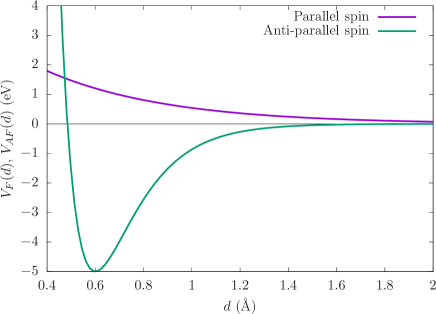
Figure 1: Atom-atom film potentials used in our calculations, both in the ferro (parallel spins) and antiferro (anti-parallel spins) configurations, see Eq. (2).

Let us particularize for the case shown in Fig. 1, where we can see that $V_{F}(d)$ does not present a minimum, while $V_{AF}(d)$ does, and let us assume that $a_{AF}\neq a_{s}$ (the lattice parameter of the substrate). Let us also assume that the lowest energy of the ferro potential exceeds the value for the antiferro case, as it is usually the case. In absence of an external field, there will be a misfit between the substrate and the film lattice parameters and, if the substrate potential is small enough, the film atoms can reconstruct.

Yet, when an external magnetic field is applied, at a certain moment the ferromagnetic configuration will be preferred energetically. Then, the advantage of reconstruction is lost, and, if the film remains coherent it will wet the substrate, i.e. it will copy its structure.

We will choose the following expressions for the three potential energy interactions:

$$V_{s}(r)=V_{s,0}\ \cos(2\pi r/a_{s}),$$

$$V_{AF}(d)=V_{AF,0}\ \Big{(}1-e^{-b_{AF}(d-a_{AF})}\Big{)}^{2}-V_{AF,0},$$

$$V_{F}(d)=V_{F,0}\ \exp(-b_{F}d),$$ (2)

i.e. a sinusoidal form for the film-substrate potential, a Morse form for the AF film potential and an exponential decay for the F film potential.

In our calculations we will employ $k_{B}=1$, measuring temperatures in energy units, which we choose to be eV. Also, the magnetic field $H$ will be measured in energy units, by making the Bohr magneton $\mu_{B}=1$. Thus, $H=1$ eV corresponds approximately to $2\cdot 10^{4}$ T when the spin values are $S_{z}=\pm\hbar/2$, which we normalize to be $s=\pm 1$. For the sake of concreteness, we will use the following parameters for the effective potentials: $a_{s}=1$ Å, $V_{s,0}=2$ eV, $V_{F,0}=4$ eV, $b_{F}=2$ Å^-1, $V_{AF,0}=5$ eV, $b_{AF}=6$ Å^-1, $a_{AF}=0.6$ Å, which constitute a reasonable choice suggested by the ab initio calculations for H chains as provided in Sec. III. Fig. 1 shows the curves for $V_{AF}(d)$ and $V_{F}(d)$ using these values.

II.1 Transfer operator approach

The physical properties of the system described by Hamiltonian (1) in equilibrium at temperature $T=\beta^{-1}$ are determined by the partition function:

$$Z=\sum_{\{r_{i},s_{i}\}}\exp\left[-\beta{\mathcal{H}}(\{r_{i},s_{i}\})\right].$$ (3)

Since the system is one-dimensional, we can write this partition function as a trace over a product of transfer matrices Baxter.82 . It is convenient to introduce new notation to simplify our expressions. Let $x_{i}=\{r_{i},s_{i}\}$ denote the multi-index which combines the position and the spin of the $i$-th atom. Then, the IFK Hamiltonian, Eq. (1) can be written as a sum of a one-body and a two-body terms

$${\mathcal{H}}=\sum_{i=1}^{N}{\mathcal{H}}^{(1)}(x_{i})+\sum_{i=1}^{N-1}{\mathcal{H}}^{(2)}(x_{i},x_{i+1}),$$ (4)

with ${\mathcal{H}}^{(1)}(x_{i})=V_{s}(r_{i})-Hs_{i}$ and ${\mathcal{H}}^{(2)}(x_{i},x_{i+1})=V_{f}(|r_{i}-r_{i+1}|,s_{i}s_{i+1})$. Let us consider $x_{i}$ to be restricted to take only a value from a finite set with $\ell$ elements. Then, we can define

$$V_{x_{i}} \equiv\exp(-\beta{\mathcal{H}}^{(1)}(x_{i})),$$

$$T_{x_{i},x_{i+1}} \equiv\exp(-\beta{\mathcal{H}}^{(2)}(x_{i},x_{i+1})),$$

$$M_{x_{i},x_{i+1}} \equiv T_{x_{i},x_{i+1}}V_{x_{i+1}},$$ (5)

leaving the dependence on the parameters ($\beta$, $H$, etc.) implied. Now, $V$ is a vector with $\ell$ components, $T$ and $M$ are matrices with dimension $\ell\times\ell$. We can then write:

$$Z =\sum_{\{x_{i}\}}V_{x_{1}}T_{x_{1},x_{2}}V_{x_{2}}T_{x_{2},x_{3}}V_{x_{3}}\cdots T_{x_{N-1},x_{N}}V_{x_{N}}$$

$$=\sum_{\{x_{i}\}}V_{x_{1}}M_{x_{1},x_{2}}M_{x_{2},x_{3}}\cdots M_{x_{N-1},x_{N}}$$

and taking into account that all $M$ matrices are equal (which need not be the case in a more general setting) we have

$$Z =\sum_{x_{1},x_{N}}V_{x_{1}}\ (M)^{N-1}_{x_{1},x_{N}}$$

$$=V^{T}\ (M)^{N-1}\ S,$$ (6)

where $S=(1,\cdots,1)^{T}$. The numerical evaluation of expression (6) is a standard problem in statistical mechanics, which may be carried out through the spectral decomposition of $M$ Baxter.82 .

Expectation values are obtained by inserting appropriate operators in the matrix product. Let us consider $\ell$ component vectors $R_{x_{i}}$ and $S_{x_{i}}$, which measure the expectation value of the position and spin of the $i$-th atom: $R_{x_{i}}=r_{i}$, $S_{x_{i}}=s_{i}$. Then,

$$\left<r_{i}\right> ={1\over Z}\sum_{\{x_{i}\}}V_{x_{1}}M_{x_{1},x_{2}}\cdots R_{x_{i}}M_{x_{i},x_{i+1}}\cdots M_{x_{N-1},x_{N}}$$

$$\left<s_{i}\right> ={1\over Z}\sum_{\{x_{i}\}}V_{x_{1}}M_{x_{1},x_{2}}\cdots S_{x_{i}}M_{x_{i},x_{i+1}}\cdots M_{x_{N-1},x_{N}}.$$ (7)

Moreover, the two-point correlators can be found in a similar way, inserting two operators, e. g. $R_{x_{i}}S_{x_{i}}$. The total magnetization $m\equiv\sum_{i}s_{i}$ can be obtained more succintly as

$$m(\beta,H)=-{1\over\beta}{\partial\log Z\over\partial H}.$$ (8)

We would like to stress the similarity between expression (6) and a matrix product state (MPS) PGarcia.07 , with the different positions of the particles, $r_{i}$, playing the role of the ancillary space, and the number $\ell$ of different positions being the bond dimension. Physically, the bond dimension of an MPS bounds the amount of information that we need to keep from the left part of the chain in order to determine the probability for the configuration of the right part. Thus, in our case this information is represented by a continuous variable, allowing for a richer behavior than in the case of the standard Ising model.

II.2 Numerical Results

The formalism presented in the previous section can be extended easily to continuous values of $r_{i}$. Yet, for practical calculations, it is convenient to consider a suitable discretization. A straightforward strategy would be to consider a length $L$ sufficiently large to hold the full chain of atoms, and to discretize it into small intervals of length $\Delta x$, studying the limit $\Delta x\to 0$. Taking spin into account, this would give a matrix size $\ell=2L/\Delta x$. In practice, this leads to working with large matrices.

In this work we will only consider coherent films, with the same density as the substrate, and with only one film atom per unit cell. Thus, each $r_{i}\in[0,a_{s}]$, with $i=1,\dots,\ell$, and the discretization step must be taken as $\Delta x=a_{s}/(\ell-1)$. Thus, the dimensions of the matrices will always be $2\ell\times 2\ell$.

We have computed exactly the partition function for an open chain, obtaining the expected positions of the film atoms making use of Eqs. (7). Fig. 2 shows these values at a low temperature, $T=0.2$ eV, for both $H=0$ and $H=5$ eV. We can see that, for $H=0$ eV the system dimerizes, i.e. presents an elementary reconstruction, doubling its unit cell. Indeed, for $H=0$ the system is antiferromagnetic, and becomes ferromagnetic, with almost all its spins parallel when $H\neq 0$ (as can also be clearly seen in Fig. 4).

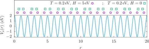
Figure 2: Average atom positions of the IFK model with $N=20$ using the parameters described in the text at very low temperature, $T=0.2$ eV, using zero magnetic field, $H=0$ eV and a large magnetic field, $H=5$ eV. Notice that the system dimerizes in absence of magnetic field. The blue line represents the film-substrate potential.

The total magnetization curve, $m(H)$ corresponding to a system with $N=50$ atoms is shown in Fig. 3 for a range of temperatures spanning from $T=0.05$ eV to $T=10$ eV. We can see that, for high temperatures, the film is completely paramagnetic, with a nearly constant slope for $m(H)$ even for $T=1$ eV. For temperatures below $T=0.2$ eV, we can observe a sharp increase in the magnetization around $H_{c}\approx\pm 2$ eV, which could correspond to a paramagnetic-ferromagnetic transition. When $T$ is below $0.1$ eV there appears another sharp increase in $m(H)$ around $H_{c}\approx\pm 1$ eV, with a plateaux between them. As a result, the critical temperature must be around $T=0.1$ eV.

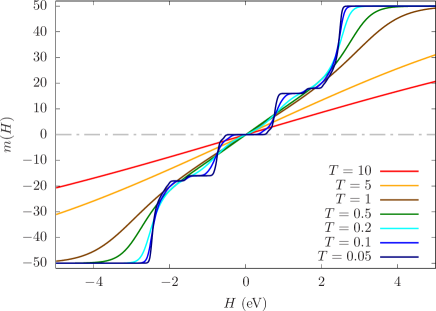
Figure 3: Magnetization curves $m(H)$ for the IFK model with $N=50$ using the parameters discussed in the text, for several temperatures, ranging from $T=0.05$ eV to $T=10$ eV.

Yet, the atomic and spin configurations of each film atom for low temperatures can be rather complex, as we can see in Fig. 4. The top panel of this figure shows the average magnetization of each atom, $\left<s_{i}\right>$, evaluated via Eq. (7), for different values of the external magnetic field, $H$ for an IFK model with $N=20$ atoms (instead of $N=50$, for easier visualization). For $H\sim 0$, the average magnetization is close to zero, increasing in amplitude near the borders, but keeping an approximate anti-ferromagnetic pattern. The outer spins, nonetheless, tends to be parallel to the external magnetic field, thus explaining the increase in the average magnetization, but holding a frustrated structure in the interior, because the number of atoms is even. The local magnetization pattern, as we can see, is complex for intermediate values of the magnetic field, becoming fully ferromagnetic only for very large values of $H$.

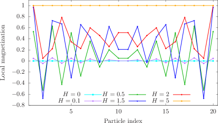
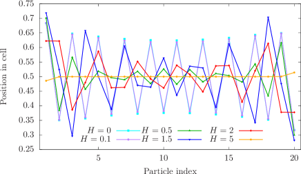
Figure 4: Top: average local magnetization of each atom in the open chain with $N=20$, for $T=0.2$ eV and different values of the magnetic field (in eV). Bottom: average position of each film atom within the unit cell of the substrate, for the same values of temperature and magnetic field.

The bottom panel of Fig. 4 shows the position of each film atom within the unit cell of the substrate, with $x=0.5$ Å denoting its center, always assuming $T=0.2$ eV and the same values as before for the external magnetic field. For $H\sim 0$, we see the alternating pattern corresponding to the dimerized reconstruction that we have shown in Fig. 2. Note that in this case the position of each alternating atom shifts about 10% the size of the unit cell. This pattern attenuates near the center as the magnetic field increases, and for $H\sim 1.5$ eV we can observe a change of the deformation phase in the right extreme of the chain, due to the fact that the rightmost extreme prefers to be polarized along the direction of the external field. For $H\sim 2$ eV, the whole pattern attenuates substantially, and for large magnetic fields we can see that the film wets the substrate, copying its structure. Notice that no frustrated structure appears in the interior. In any case, we would like to stress that a chain with $N=21$ atoms will yield the opposite behavior for both the magnetization and the positions.

In order to obtain a full physical characterization of our system let us consider the behavior of the magnetic susceptibility $\chi$, defined as

$$\chi=\left.{\partial m\over\partial H}\right|_{H=0},$$ (9)

which is plotted in Fig. 5, for different system sizes. We observe that, for low tempeatures, the susceptibility $\chi\approx 0$, which is consistent with the predicted antiferromagnetic (AF) behavior. At a finite temperature value $T\sim 0.15$ eV we observe a sharp rise, whose peak height depends on the system size $L$. Furthermore, beyond the peak the susceptibility decays approximately as $T^{-1}$, corresponding to the Curie law of paramagnetism. This behavior is consistent with a second-order phase transition from an antiferromagnetic at low temperatures towards a paramagnetic behavior. This type of phase transition is sometimes accompanied by structural changes in Nature Zu.16 ; Liu.20 .

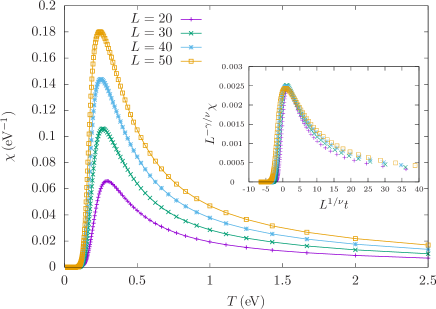
Figure 5: Magnetic susceptibility as a function of the temperatures for different system sizes. Inset: finite-size collapse of the susceptibility curves following Eq. (10).

The nature of the phase transition and its critical exponents can be obtained through a finite-size scaling Newman.MCbook , assuming that in the vicinity of the transition the susceptibility follows the law

$$\chi(T)\approx L^{\gamma/\nu}F(L^{1/\nu}t),$$ (10)

where $L$ is the system size ($L\propto N$ in our case), $t=(T-T_{c})/T_{c}$ is the reduced temperature, $T_{c}$ is the critical temperature, $\nu$ and $\gamma$ are the critical exponents associated to the correlation length, $\xi\sim t^{-\nu}$, and the susceptibility, $\chi\sim t^{-\gamma}$. The inset of Fig. 5 shows that an accurate collapse is obtained through $T_{c}\approx 0.11$ eV, $\nu\approx 2.1$ and $\gamma\approx 2.31$.

Finding the mechanism behind these exponents is not an easy task. Yet, we may conjecture that they may correspond to an Ising model with long-range interactions Hiley.65 ; Glumac.89 ; Wragg.90 ; Cannas.95 , i.e. a Hamiltonian of the type

$${\cal H}=\sum_{i<j}{1\over|i-j|^{\alpha}}s_{i}s_{j},$$ (11)

where $\alpha$ is the decaying exponent for the coupling constants. Indeed, the critical exponent for this model depends on $\alpha$. In the range $\alpha\in(1,2)$ we find values for $\nu$ and $\gamma$ which are compatible with our results Wragg.90 ; Cannas.95 .

The rich phase diagram of the Frenkel-Kontorova model is determined by two parameters: the lattice parameter misfit and the ratio between the film and substrate potentials. In our IFK case, there are two different film potentials, which give rise to two different possible ratios. Yet, both are simultaneously changed when the amplitude of the substrate potential is varied. Indeed, a change in $V_{s,0}$ can induce a further phase transition, as we will describe below.

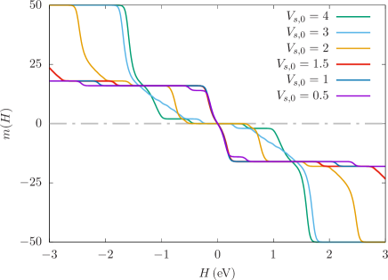
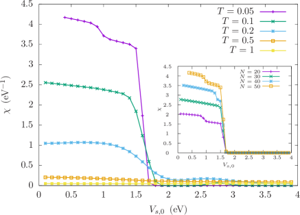
Figure 6: Top: magnetization as a function of the applied field, $m(H)$ using $N=50$ and $T=0.05$ for different values of $V_{s,0}$ (in Å). For $V_{s,0}$ above a critical value all magnetization curves present a finite plateau at $H=0$, which is a fingerprint of the antiferromagnetic phase. Bottom: susceptibility $\chi$ (at $H=0$) as a function of $V_{s,0}$, using $N=50$ and different values of $T$ (in eV). Notice that the susceptibility falls to zero above the aforementioned critical value unless the temperature is high enough. The inset shows the susceptibility as a function of $V_{s,0}$ for different system sizes $N$ using $T=0.05$.

In Fig. 6 (top) we can see the expected value of the magnetization as a function of the applied magnetic field at very low temperature ($T=0.05$) using $N=50$ atoms. All the parameters are the same as in the previous calculations, except for the substrate potential amplitude, $V_{s,0}$, which was varied around its original value of 2 eV. We should pay special attention to the vicinity of the $H=0$ value, where we can see a finite plateau for high values of $V_{s,0}$ and a finite slope for low values. This plateau is a fingerprint of the antiferromagnetic phase, which can be seen to disappear for weak substrate potentials (check Fig. 3).

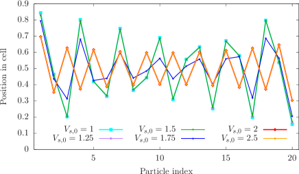
Figure 7: Atomic positions at $H=0$ for a chain with $N=20$ for easier visualization, using $T=0.05$ eV and different values of $V_{s,0}$. Notice that cases $V_{s,0}=1$, 1.25 and 1.5 eV collapse nearly exactly, because they correspond to the same structural phase, and the same can be claimed for $V_{s,0}=2$ and 2.5 eV, where the antiferromagnetic phase induces dimerization.

Yet, we can not simply claim that for low values of $V_{s,0}$ the system reaches a paramagnetic phase. Indeed, the plateau exists for all values of $V_{s,0}$, but it shifts away from $H=0$ when the substrate potential is too weak. In the bottom panel of Fig. 6 we can see the dependence of the magnetic susceptibility, $\chi$, (defined in Eq. (9)) with $V_{s,0}$ for different temperatures. We can observe a sudden drop for low temperatures at a value $V_{s,0}\approx 1.75$ eV, while for high temperatures the system becomes paramagnetic and $V_{s,0}$ becomes almost irrelevant to determine $\chi$. The inset shows how the $T=0.05$ eV curve changes when we choose different system sizes, and allows us to claim that the jump in $\chi$ grows with $N$.

It is natural to ask whether this new transition has a visible structural impact in the nanowire. We can see that this is indeed the case in Fig. 7, which shows the positions of the atoms within the unit cell, in similarity to Fig. 4 (bottom), for different values of $V_{s,0}$, using always $N=20$ (for easier visualization), $H=0$ and $T=0.05$ eV. Indeed, the antiferromagnetic phase always corresponds to a nearly perfect dimerization. Yet, for weak substrate potentials, $V_{s,0}<2$ eV we observe a large deviation, with a period 3 modulation superimposed on a smooth decreasing trend from the boundaries. This plot shows that the magnetic structure interacts in a very non-trivial way with the Frenkel-Kontorova degrees of freedom, giving rise to novel phenomena.

We would like to stress that our calculations always use open boundaries, since they are the most natural setup for an atomic nanowire. Moreover, the end atoms are always less attached to the chain and are more susceptible to the action of an external field. Moreover, also the parity of the number of atoms is relevant. Indeed, if $N$ is even both end atoms can not align simultaneously with the external field if the effective spin-spin interaction is antiferromagnetic.

III Ab Initio Calculations

In this section we show proof-of-principle ab initio calculations for atomic chains (i.e. nanowires) performed with DFT. We have chosen two different atomic species: on one hand, we have considered hydrogen (H), because it gives rise to simple calculations. Moreover, we have performed computations using iron (Fe), in order to compare with previous ab initio studies of nanowires of transition metals Sargolzaei ; Tung ; Zarechnaya .

In both cases, we have built a chain of $N=8$ atoms with a total length $L=a_{s}N$, where $a_{s}$ is the substrate lattice parameter, and assuming periodic boundary conditions. Crucially, the expected value of the total spin of the chain is fixed. For H, we have considered the cases of $\left<S_{z}\right>=0$, $2\hbar$ and $4\hbar$ which, for $N=8$ atoms, correspond to zero, half and full magnetizations. On the other hand, for Fe we have considered $\left<S_{z}\right>=0$, $8\hbar$, $\dfrac{27}{2}\hbar$ and $16\hbar$, implying that the total magnetization is a fraction of its maximal possible value: $0$, $0.25$, $0.42$ or $0.5$. In this way, we will be able to characterize the behavior of the atom-atom film interaction in absence of external magnetic field (zero magnetization) or in the presence of external fields of given different strengths. In order to simplify the calculations, the substrate potential is absent from our calculations, except through the imposed substrate lattice parameter.

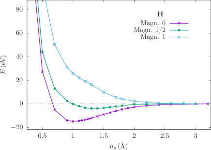
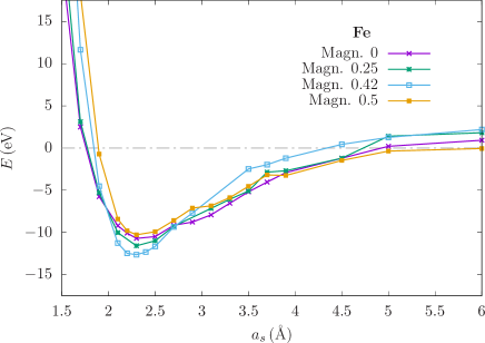
Figure 8: DFT calculations of the total energy of a H (top) or Fe (bottom) chain of 8 atoms as a function of the lattice spacing, using periodic boundary conditions for several values of the magnetization fraction, i.e. $\left<S_{z}\right>$ normalized by the maximal possible magnetization, $n_{e}\hbar/2$. In the case of Fe, notice the complex pattern of energy curves. Indeed, the optimal magnetization is non-zero for a range of values of $a_{s}$, while it may be zero for $a_{s}\in(2.8,3.5)$ Å.

Electronic calculations were performed using the SIESTA code Soler.02 , keeping fixed the chain structure during the calculations, while the electronic part is relaxed. The exchange and correlation potential was described using the Perdew, Burke, and Ernzerhof (PBE) functional Perdew.96 . This functional was already used in previous works on H₂ adsorption on single and double aluminium clusters doped with vanadium or rhodium Vanbuel.17 ; Vanbuel.19 ; Vanbuel.18 ; Jia.18 . The core interactions were accounted for by means of norm conserving scalar relativistic pseudopotentials Troullier.91 in their fully nonlocal form Kleinman.82 , generated from the atomic valence configuration $1s^{1}$ for H and 4$s^{2}$3$d^{6}$ for Fe. The core radii for the $s$ orbital of H is $1.25$ a.u. and for the $s$ and $d$ orbitals of Fe is 2.0 a.u. The matrix elements of the self-consistent potential were evaluated by integrating in an uniform grid. The grid fineness is controlled by the energy cutoff of the plane waves that can be represented in it without aliasing (150 Ry in this work). Flexible linear combinations of numerical pseudo-atomic orbitals (PAO) are used as the basis set, allowing for multiple-$\zeta$ and polarization orbitals. To limit the range of PAOs, they were slightly excited by a common energy shift (0.005 Ry in this work) and truncated at the resulting radial node, leading to a maximum cutoff radii for the $s$ orbitals of 6.05 a.u. for H and 7.515 a.u. for Fe. The chain structure remains fixed during the calculations, while the electronic part is relaxed.

As commented, in order to make proper comparisons wit our previous results regarding the IFK model, and for the sake of saving computational effort, we have considered two types of calculations assuming fixed 1D chains (with 8 atoms of H or Fe), keeping constant the expected value of the total spin of the chain, as discussed above. Firstly, we have evaluated the total energy of the chains as a function of the varying distance between adjacent atoms. Secondly, we have assumed a fixed lattice parameter for the unit cell and evaluated the energy of dimerized chains for distinct values of the dimerization parameter.

In the first numerical experiment, we have calculated the total energy of the chain as a function of the substrate lattice spacing, $a_{s}$, assuming that the film copies the substrate, for all magnetizations discussed previously. The results are presented in Fig. 8, where the top panel represents the results for the H chains and the bottom panel those for the Fe ones. Notice that the energy zero has been set to the (lowest) energy obtained for the largest value of $a_{s}$ for a better visualization. The results are obtained for the selected values of the magnetization fraction, i.e. the expected value of the total spin of the chain, $\left<S_{z}\right>$, divided by the maximal possible value, $n_{e}\hbar/2$, where $n_{e}$ is the total number of electrons (8 for H and 64 for Fe). We can observe a similar behavior to the potentials between the film atoms in Fig. 1. For hydrogen, we see that in the absence of an external magnetic field the system will choose the configuration with zero magnetization, with an energy minimum around a value $a_{s}\approx 1$ Å. As the magnetic field increases, the magnetic contribution to the total energy will eventually favor the upper curves, corresponding to higher total spin. For Fe, on the other hand, for no magnetic field the preferred magnetization is $\left<S_{z}\right>\neq 0$, and the behavior of the energy curves are sufficiently different to suggest that the presence of external magnetic fields will give rise to different film interaction potentials. The results for H (top panel of Fig. 8) inspired our choice of values of the physical parameters of the IFK model discussed in Sec. II.

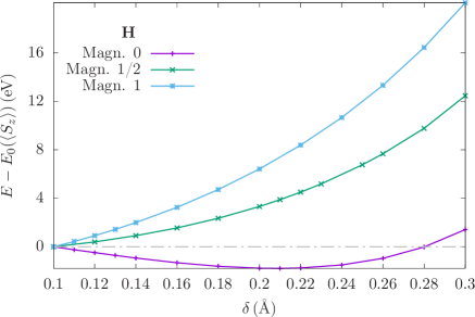
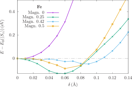
Figure 9: Energy of the same chains as in Fig. 8 when allowed to dimerize, as a function of the dimerization parameter $\delta$, using $a_{s}=1.0$ Å for H (top) and $a_{s}=2.3$ Å for Fe (bottom), for the same values of the magnetization $\left<S_{z}\right>$, as in Fig. 8. The curves are vertically shifted a quantity $E_{\delta=0}(\left<S_{z}\right>)$ for a better comparison.

For the second computer experiment we fix the lattice parameter of the substrate to the minimun obtained in the Fig. 8 ($a_{s}=1.0$ Å for H and $a_{s}=2.3$ Å for Fe) and we impose a dimerization on the atomic positions of the chain, according to the rule:

$$r_{n}=na_{s}+(-1)^{n}\delta.$$ (12)

By varying the dimerization parameter $\delta$ we get the results shown in Fig. 9, with the top panel again devoted to H and the bottom panel to Fe, as in Fig. 8. Note that, for better comparison, we have displaced vertically the energies for each magnetization by $E_{\delta=0}(\left<S_{z}\right>)$, labeled as $E_{0}(\left<S_{z}\right>)$. As we can see, in the case of zero magnetization, the H energy presents a minimum at a dimerization parameter $\delta\approx 0.21$ Å, thus confirming our conjecture: the film will reconstruct in this case, if the substrate potential is not too strong. On the other hand, for half and full magnetization we can see that the energy tends to a minimum for zero dimerization, showing that, at least, this reconstruction scheme does not reduce the total energy. Thus, we are allowed to conjecture, based on the presented data, that this system will show different structures for zero and for high magnetic fields.

This phenomenon is even more salient for Fe, as we can see in the bottom panel of 9. The equilibrium value of the dimerization parameter is strongly dependent on the magnetization. Thus, we are led to conjecture that the imposition of a strong external magnetic field may induce structural changes.

IV Physical picture

The combination of ab initio calculations and statistical mechanics provides a unified physical picture of the complex physical behavior of absorbed nanowires in presence of external magnetic fields.

The simplest scenario corresponds to hydrogen atoms on an inert and rigid substrate, as shown both using the IFK model and DFT calculations. In absence of an external field and for weak substrate potentials, the chain will reconstruct while presenting an antiferromagnetic structure. This reconstruction can be avoided by three different routes: increasing the temperature, increasing the external magnetic field or diminishing the ratio between the film and the substrate potentials. The antiferromagnetic to paramagnetic transition present the usual features associated to a long-range Ising model.

We should ask about the ranges for the temperature and the magnetic fields for which the phenomena discussed in this article will take place. In Sec. II we have employed numerical values for the physical parameters chosen to resemble the effective potentials in the H chain. In that case, we can see that the critical temperature $T_{c}\sim 0.1$ eV $\sim 1200$ K, and the magnetic field $H\sim 1$ eV $\sim 2\cdot 10^{4}$ T, which is simply too large for any practical purposes. In general terms, if the film is composed of atoms or molecules with a large magnetic moment, the necessary magnetic field will be reduced by the same factor. Yet, the complexity of the energy curves in multielectronic atoms can play in our favor, as it may be the case of Fe. As we see in Figs. 8 (bottom), the energy curve for zero magnetization shows the lowest values of the energies for $a_{s}$ in a range from $2.8$ to $3.5$ Å. Choosing an appropriate $a_{s}$, the energy difference between the curves corresponding to different magnetization levels can be made arbitrarily low, thus allowing a small external magnetic field to provide the necessary difference to induce a phase transition.

The nanowire of Fe atoms deserves further attention. The potential energy curves shown in the bottom panels of Figs. 8 and 9 suggest that the IFK model should be extended in order to provide a full physical explanation of this case. The straightforward procedure would be to fit the $V_{F}$ and $V_{AF}$ potentials to the numerical data obtained from DFT, but it is easy to understand that this will not be enough. The intrincate behavior of iron atoms can not be accounted for using classical Ising spins ($S_{z}=\pm 1$). A classical statistical model would require, at least, the use of or Heisenberg spins Baxter.82 .

Our calculations have shown that the general mechanism provided in this article can work in real materials. Of course, these calculations are only a proof-of-principle, using simple geometries. Indeed, it is natural for atomic chains to dimerize due to Peierls instability Peierls , although the dimerization in our case has a different origin. Further calculations, using more realistic materials, are still needed in order to make any experimental proposal to observe the predicted reconstruction effects. We should remark that our results are in line with those of previous works Tung ; Zarechnaya , which provide some theoretical evidence of magnetic crossovers in transition atoms, as the preferred magnetization varies as a function of the atomic distances. In some cases, the chains are more stable when displayed along a zig-zag geometry Tung .

An interesting experimental route may be provided by the use of ultracold atoms in optical lattices, since most parameters can be easily engineered, and thus the different transitions can be observed just tuning the intensities of the laser beams GarciaMata.07 ; Lewenstein.12 .

V Conclusions and Further Work

We have put forward the following question: can nanowires reconstruct differently in the presence of external magnetic (or electric) fields? After our calculations, we can conjecture that this can indeed be the case. We have performed illustrative ab initio calculations using DFT, showing that this possibility exists for two types of atoms: hydrogen and iron.

Furthermore, we have proposed a statistical mechanical model, which is an Ising-like extension of the Frenkel-Kontorova model, the IFK model, in which film atoms interact differently when their spin variables are the same or opposite. We have extracted some salient physical consequences in the 1D case, using reasonable forms for the film potentials and a sinusoidal form for the interaction with the substrate, showing a rich behavior with an antiferromagnetic-paramagnetic second-order phase transition at a finite value of the temperature. It is relevant to discuss how an Ising-like model can give rise to a phase transition at finite temperature in 1D, since they are forbidden for short-ranged Ising models due to entropic considerations Huang . The reason is as follows: we may integrate out the spatial degrees of freedom, giving rise to an effective Ising model for the spins presenting long-range interactions. Indeed, the critical exponents that we have found allow us to conjecture that, indeed, our model behaves as a long-range Ising model in 1D.

The mechanism described in this paper bears some similarity with colossal magnetoresistance (CMR), where metallic ferromagnetic regions co-exists with insulating antiferromagnetic ones, due to the presence of quenched disorder Dagotto.05 . An external magnetic field will favor the ferromagnetic regions, thus allowing them to reach the percolation threshold and decrease the effects the disorder and the resistance dramatically.

It is likely that, as we increase the magnetic field, the antiferromagnetic configuration will not become directly unstable, but metastable. In other terms: the transition may be of first order. This implies that, as one cycles over a range of magnetic fields, we will obtain a hysteresis cycle.

Throughout this article we have used a magnetic field to force the change in reconstruction. In principle, electric fields can also be used, in the case of film atoms or molecules with a permanent electric dipole.

In order to proceed with this line of research, there are several complementary routes. First of all, it will be very interesting to consider how some characteristic features of the FK model extend to the IFK case, such as the commensurate-incommensurate transition or the presence of defects (e.g. kinks). Moreover, it is worth to develop further the statistical mechanics of the IFK, both in 1D and 2D, where the physical properties should be richer and reconstruction would be more experimentally feasible. In order to obtain experimental confirmation of our results, the choice of the correct materials is of paramount importance. We can obtain some guidance from numerical simulations combining DFT and statistical mechanical tools in order to select those which will present a critical magnetic field within the experimental range. In this case, more complicated potential curves will be required, as it is shown by the DFT results for Fe, which may be correctly described using e.g. Heisenberg spins. After some suitable materials have been chosen and characterized, we intend to make a concrete experimental proposal.

- (1) K. Oura, V.G. Lifshits, A.A. Saranin, A.V. Zotov, M. Katayama, Surface science: an introduction, Springer (2003).
- (2) H. Brune, H. Röder, C. Boragno, K. Kern, Strain relief at hexagonal-closed-packed interfaces, Phys. Rev. B 49, 2997 (1994).
- (3) T.J. Krzyzewski, P.B. Joyce, G.R. Bell, T.S. Jones Surface morphology and reconstruction changes during heteroepitaxial growth of InAs on GaAs(0 0 1)-(24), Surf. Sci. 482, 891 (2001).
- (4) P. Raghani, Investigating complex surface phenomena using density functional theory, chapter in Practical Aspects of Computational Chemistry III, Ed. J. Leszczynski and M.K. Shukla, Springer (2014).
- (5) T. Makita et al., Structures and electronic properties of aluminum nanowires, J. Chem. Phys. 119, 538 (2003).
- (6) C. Noguera, J. Goniakowski, Structural phase diagrams of supported oxide nanowires from extended Frenkel-Kontorova models of diatomic chains, J. Chem. Phys. 139, 084703 (2013).
- (7) Y. Yu, F. Cui, J. Sun, P. Yang, Atomic structure of ultrathin gold nanowires, Nano Lett. 16, 3078 (2016).
- (8) S. Lazarev et al., Structural changes in a single GaN nanowire under applied voltage bias, Nano Lett. 18, 5446 (2018).
- (9) R. Pushpa, J. Rodriguez-Laguna, S.N. Santalla, Reconstruction of the second layer of Ag on Pt(111), Phys. Rev. B 79, 085409 (2009).
- (10) M. Sargolzaei, S.S. Ataee, First principles study on spin and orbital magnetism of 3d transition metal monatomic nanowires (Mn, Fe and Co), J. Phys.: Condens. Matter 23, 125301 (2011).
- (11) J.C. Tung, G.Y. Guo, Systematic ab initio study of the magnetic and electronic properties of all 3d transition metal linear and zigzag nanowires, Phys. Rev. B 76, 094413 (2007).
- (12) E.Yu. Zarechnaya, N.V. Skorodumova, S.I. Simak, B. Johansson, E.I. Isaev, Theoretical study of linear monoatomic nanowires, dimer and bulk of Cu, Ag, Au, Ni, Pd and Pt, Comp. Mat. Sci. 43, 522 (2008).
- (13) , J. Frenkel, T. Kontorova, On the theory of plastic deformation and twinning, Phys. Zeit. der Sowjetunion 13, 1 (1938).
- (14) J. Frenkel, T. Kontorova, On the theory of plastic deformation and twinning, J. Phys. (USSR) 1, 137 (1939).
- (15) O.M. Braun, Y.S. Kivshar, The Frenkel-Kontorova model: concepts, methods and applications, Springer (2004).
- (16) M. Mansfield, R.J. Needs, Application of the Frenkel-Kontorova model to surface reconstructions, J. Phys.: Condens. Matter 2, 2361 (1990).
- (17) J. Rodriguez-Laguna, S.N. Santalla, Vertically extended Frenkel-Kontorova model: a real space renormalization group study, Phys. Rev. B 72, 125412 (2005).
- (18) B. Hu, B. Li, Quantum Frenkel-Kontorova Model, Physica A 288, 81 (2000).
- (19) R. Pushpa, S. Narasimhan, Reconstruction of Pt(111) and domain patterns on close-packed metal surfaces, Phys. Rev. B 67, 205418 (2003).
- (20) B. Barbara et al., Spontaneous magnetoelastic distortion in some rare earth-iron Laves phases, Physica 86, 155 (1977).
- (21) R. Toft-Petersen et al., Magnetoelastic phase diagram of TbNi2B2C, Phys. Rev. B 97, 224417 (2018).
- (22) R.D. Mattuck, M.W.P. Strandberg, Spin-Phonon Interaction in Paramagnetic Crystals, Phys. Rev. 119, 1204 (1960).
- (23) O. Tschernyshyov, G.W. Chern, Spin-lattice coupling in frustrated antiferromagnets, chapter in C. Lacroix et al. (eds.) Introduction to frustrated magnetism, Springer series in solid-state sciences 164 (2011).
- (24) Y. Teraoka, H. Ishibashi, Y. Tabata, Surface reconstruction and surface magnetism, J. Magn. & Magn. Mat. 104, 1701 (1992).
- (25) J.M. Gallego, D.O. Boerma, R. Miranda, F. Ynduráin, 1D Lattice Distortions as the Origin of the (22)p4gm Reconstruction in ’-Fe4N(100): A Magnetism-Induced Surface Reconstruction, Phys. Rev. B 95, 136102 (2005).
- (26) H. Tang et al., Magnetic Reconstruction of the Gd(0001) Surface, Phys. Rev. Lett. 71, 444 (1993).
- (27) A. Rettori, L. Trallori, P. Politi, M.G. Pini, M. Macciò, Surface magnetic reconstruction, J. Magn. & Magn. Mat. 140, 639 (1995).
- (28) M. Macciò, M.G. Pini, L. Trallori, P. Politi, A. Rettori, Surface magnetic reconstruction with enhanced magnetic order, Phys. Lett. A 205, 327 (1995).
- (29) S.L. Zhang et al., Direct Observation of Twisted Surface skyrmions in Bulk Crystals, Phys. Rev. Lett. 120, 227202 (2018).
- (30) R. Baxter, Exactly solved models in statistical mechanics, Academic Press (1982).
- (31) D. Pérez-García, F. Verstraete, J.I. Cirac, Matrix Product State Representations, Quantum Inf. Comp. 7, 401 (2007).
- (32) L. Zu et al., A first-order antiferromagnetic-paramagnetic transition induced by structural transition in GeNCr3, App. Phys. Lett. 108, 031906 (2016).
- (33) C. Liu et al., First-order magnetic transition induced by structural transition in hexagonal structure, J. Magn. Magn. Mat. 494, 165821 (2020).
- (34) M.E.J. Newman, G.T. Barkema, Monte Carlo methods in statistical physics, Oxford Univ. Press (1991).
- (35) B.J. Hiley, G.S. Joyce, The Ising model with long-range interactions, Proc. Phys. Soc. 85, 493 (1965).
- (36) Z. Glumac, K. Uzelac, Finite-range scaling study of the 1D long-range Ising model, J. Phys. A: Math. Gen. 22, 4439 (1989).
- (37) M.J. Wragg, G.A. Gehring, The Ising model with long-range ferromagnetic interactions, J. Phys. A: Math. Gen. 23, 2157 (1990).
- (38) S.A. Cannas, One-dimensional Ising model with long-range interactions: a renormalization group treatment, Phys. Rev. B 52, 3034 (1995).
- (39) J.M. Soler, E. Artacho, J.D. Gale, A. García, J. Junquera, P. Ordejón, D. Sánchez-Portal, The SIESTA method for ab initio order-N materials simulation, J. Phys.: Condens. Matter 14, 2745 (2002).
- (40) J.P. Perdew, K. Burke, M. Ernzerhof, Generalized Gradient Approximation Made Simple, Phys. Rev. Lett. 77, 3865 (1996).
- (41) J. Vanbuel, E.M. Fernández, P. Ferrari, S. Gewinner, W. Schöllkopf, L.C. Balbás, A. Fielicke, E. Janssens, Hydrogen Chemisorption on Singly Vanadium‐Doped Aluminum Clusters, Chemistry: a European journal 23, 15638 (2017).
- (42) J. Vanbuel, E.M. Fernández, M. Jia, P. Ferrari, W. Schöllkopf, L.C. Balbás, M.T. Nguyen, A. Fielicke, E. Janssens, Hydrogen Chemisorption on Doubly Vanadium Doped Aluminum Clusters, Z. Phys. Chem 233, 799 (2019).
- (43) J. Vanbuel, M. Jia, P. Ferrari, S. Gewinner, W. Schöllkopf, M.T. Nguyen, A. Fielicke, E. Janssens, Competitive Molecular and Dissociative Hydrogen Chemisorption on Size Selected Doubly Rhodium Doped Aluminum Clusters, Topics in Catalysis 61, 62 (2018).
- (44) M. Jia, J. Vanbuel, P. Ferrari, E.M. Fernández, S. Gewinner, W. Schöllkopf, M.T. Nguyen, A. Fielicke, E. Janssens, Size Dependent H2 Adsorption on AlnRh+ ( 1–12) Clusters, The Journal of Physical Chemistry C 122, 18247 (2018).
- (45) N. Troullier, J.L. Martins, Efficient pseudopotentials for plane-wave calculations, Phys. Rev. B 43, 1993 (1991).
- (46) L. Kleinman, D.M. Bylander, Efficacious Form for Model Pseudopotentials, Phys. Rev. Lett. 48, 1425 (1982).
- (47) R. Peierls, More surprises in theoretical physics, Princeton Series in Physics (1991).
- (48) I. García-Mata, O.V. Zhirov, D.L. Shepelyansky, Frenkel-Kontorova model with cold trapped ions, Eur. Phys. J. D 41, 325 (2007).
- (49) M. Lewenstein, A. Sanpera, V. Ahufinger, Ultracold atoms in optical lattices, Oxford University Press (2012).
- (50) K. Huang, Statistical Mechanics, John Wiley & Sons (1987).
- (51) E. Dagotto, Complexity in Strongly Correlated Electronic Systems, Science 309, 257 (2005).