Rejection-Based Simulation of Non-Markovian Agents on Complex Networks

Abstract

Stochastic models in which agents interact with their neighborhood according to a network topology are a powerful modeling framework to study the emergence of complex dynamic patterns in real-world systems. Stochastic simulations are often the preferred—sometimes the only feasible—way to investigate such systems. Previous research focused primarily on Markovian models where the random time until an interaction happens follows an exponential distribution.

In this work, we study a general framework to model systems where each agent is in one of several states. Agents can change their state at random, influenced by their complete neighborhood, while the time to the next event can follow an arbitrary probability distribution. Classically, these simulations are hindered by high computational costs of updating the rates of interconnected agents and sampling the random residence times from arbitrary distributions.

We propose a rejection-based, event-driven simulation algorithm to overcome these limitations. Our method over-approximates the instantaneous rates corresponding to inter-event times while rejection events counter-balance these over-approximations. We demonstrate the effectiveness of our approach on models of epidemic and information spreading.

1 Introduction

Computational modeling of dynamic processes on complex networks is a thriving research area [1, 2, 3]. Arguably, the most common formalism for spreading processes is the continuous-time SIS model and its variants [4, 5, 6]. Generally speaking, an underlying contact network specifies the connectivity between nodes (i.e., agents) and each agent occupies one of several mutually exclusive (local) states (or compartments). In the well-known SIS model, these states are susceptible (S) and infected (I). Infected nodes can recover (become susceptible again) and propagate their infection to neighboring susceptible nodes.

SIS-type models have shown to be extremely useful for analyzing and predicting the spread of opinions, rumors, and memes in online social networks [7, 8] as well as the neural activity [9, 10], the spread of malware [11], and blackouts in financial institutions [12, 13].

Previous research focused mostly on models where the probability of an event (e.g. infection or recovery) happening in the next (infinitesimal) time unit is constant, i.e. independent of the time the agent has already spent in its current state. We call such agents memoryless and the corresponding stochastic process Markovian. The semantics of such a model can be described using a so-called (discrete-state) continuous-time Markov chain (CTMC).

One particularly important consequence of the memoryless property is that the random time until an agent changes its state, either because of an interaction with another agent or because of a spontaneous transition, follows an exponential distribution. The distribution of this residence time is parameterized by an (interaction-specific) rate $\lambda\in\mathbb{R}_{\geq 0}$ [4]. Each agent has an associated event-modulated Poisson process whose rate depends on the agent’s state and the state of its neighbors [14]. For instance, infection of an agent increases the rate at which its susceptible neighbors switch to the infected state.

However, exponentially distributed residence times are an unrealistic assumption in many real-word systems. This holds in particular for the spread of epidemics [15, 16, 17, 18, 19], for the diffusion of opinions in online social networks [20, 21], and interspike times of neurons [22] as empirical results show. However, assuming time delays that can follow non-exponential distributions complicate the analysis of such processes and typically only allow Monte-Carlo simulations, which suffer from high computational costs.

Recently, the Laplace-Gillespie algorithm (LGA) for the simulation of non-Markovian dynamics has been introduced by Masuda and Rocha in [14]. It is based on the non-Markovian Gillespie algorithm by Boguná et al (nMGA) [23] and minimizes the costs of sampling inter-event times. However, both methods require computationally expensive updating of an agent’s neighborhood in each simulation step, which renders them inefficient for large-scale networks. In the context of Markovian processes on networks, it has recently been shown that rejection-based simulation can overcome this limitation [24, 25, 26].

Here, we extend the idea of rejection-based simulation to non-Markovian networked systems, proposing RED-Sim, a rejection-based, event-driven simulation approach. Specifically, we combine three ideas to obtain an efficient simulation of non-Markovian processes: (i) we express the distributions of inter-event times through time-varying instantaneous rates, (ii) we sample events based on an over-approximation of these rates and compensate via a rejection step, and (iii) we use a priority queue to sample the next event. The combination of these elements makes it possible to reduce the time-complexity of each simulation step. Specifically, if an agent changes its state, no update of the rate of neighboring agents is necessary. This comes at the costs of rejection events to counter-balance missing information about the neighborhood. However, using a priority queue renders the computational burden of each rejection event very small.

The remainder of the paper is organized as follows: We describe our framework for non-Markovian dynamics in Section 2 and provide a review of previous simulation approaches in Section 3. Next, we propose our rejection-based simulation algorithm in Section 4. Section 5 presents numerical results and we conclude our work in Section 6.

2 Multi-Agent Model

This section introduces the underlying formalism to express agent-based dynamics on networks. Let $\mathcal{G}=(\mathcal{N},\mathcal{E})$ be a an undirected, finite graph without self-loops, called contact network. Nodes $n\in\mathcal{N}$ are also referred to as agents.

2.0.1 Network State.

The current state of a network $\mathcal{G}$ is described by two functions:

• $S:\mathcal{N}\rightarrow\mathcal{S}$ assigns to each agent $n$ a local state $S(n)\in\mathcal{S}$, where $\mathcal{S}$ is a finite set of local states (e.g., $\mathcal{S}=\{\texttt{S},\texttt{I}\}$ for the SIS model);

• $R:\mathcal{N}\rightarrow\mathbb{R}_{\geq 0}$, describes the residence time of each agent, i.e. the time since the last change of state of the agent.

We say that an agent fires when it changes its state and refer to the remaining time until it fires as its time delay. The neighborhood state $M(n)$ of an agent $n$ is a multi-set containing the states of all neighboring agents together with their respective residence times:

$$M(n)=\Big{\{}\big{(}S(n^{\prime}),R(n^{\prime})\big{)}\;\big{|}\;(n,n^{\prime})\in\mathcal{E}\Big{\}}\;.$$

The set of all possible neighborhood-states of all agents in a given system is denoted by $\mathcal{M}$.

2.0.2 Network Dynamics.

The dynamics of the network is described by assigning to each agent $n$ two functions $\phi_{n}$ and $\psi_{n}$:

• $\phi_{n}:\mathcal{S}\times\mathbb{R}_{\geq 0}\times\mathcal{M}\rightarrow\mathbb{R}_{\geq 0}$ defines the instantaneous rate of $n$, i.e. if $\lambda=\phi_{n}\big{(}S(n),R(n),M(n)\big{)}$, then the probability that $n$ fires in the next infinitesimal time interval $t_{\Delta}$ is $\lambda t_{\Delta}$;

• $\psi_{n}:\mathcal{S}\times\mathbb{R}_{\geq 0}\times\mathcal{M}\rightarrow P_{\mathcal{S}}$ determines the state probabilities when a transition occurs. Here, $P_{\mathcal{S}}$ denotes the set of all probability distributions over $\mathcal{S}$. Hence if $p=\psi_{n}\big{(}S(n),R(n),M(n)\big{)}$, then, when agent $n$ fires, the next local state is $s$ with probability $p(s)$.

Note that we do not consider cases of pathological behavior here, e.g. where $\phi_{n}$ is defined in such a way that an infinite amount of simulation steps is possible in finite time.

A multi-agent network model is completely specified by a tuple $(\mathcal{G},$ $\mathcal{S},$ $\{\phi_{n}\},$ $\{\psi_{n}\},S_{0})$, where $S_{0}$ denotes a function that assigns to each node an initial state.

2.0.3 Example.

In the classical SIS model we have $\mathcal{S}=\{\texttt{S},\texttt{I}\}$ and $\phi$ and $\psi$ are the same for all agents, i.e.,

$$\phi_{n}(s,t,m)=\begin{cases}c_{r}\text{\hskip 61.17325pt if $s=\texttt{I}$}\\ c_{i}\sum\limits_{s^{\prime},t^{\prime}\in m}\mathbbm{1}_{\texttt{I}}(s^{\prime})\text{ \; if $s=\texttt{S}$}\end{cases}\hskip 2.84544pt\psi_{n}(s,t,m)=\begin{cases}\mathbbm{1}_{\texttt{S}}\text{\hskip 8.5359pt if $s=\texttt{I}$}\\ \mathbbm{1}_{\texttt{I}}\text{\hskip 8.5359pt if $s=\texttt{S}$}\end{cases}$$

Here, $c_{i},c_{r}\in\mathbb{R}_{\geq 0}$ denote the infection and recovery rate constants, respectively. Note that the infection rate is proportional to the number of infected neighbors whereas the rate of recovery is independent from neighboring agents. Moreover, $\mathbbm{1}_{s}:\mathcal{S}\rightarrow\{0,1\}$ maps a state $s^{\prime}$ to one iff $s=s^{\prime}$ and to zero otherwise. The model is Markovian as neither $\phi$ nor $\psi$ depend on the residence time of any agent.

2.1 Semantics

We will specify the semantics of a multi-agent model by describing a stochastic simulation algorithm that generates trajectories of the system. It is based on a race condition among agents: each agent picks a random time until it will fire, but only the one with the shortest time delay wins and changes its state.

2.1.1 Time Delay Density.

Assume that $t_{\Delta}$ is the time increment of the algorithm. We define for each $n$ the effective rate $\lambda_{n}(t_{\Delta})$ as

$$\begin{array}[]{l}\lambda_{n}(t_{\Delta})=\phi_{n}\Big{(}S(n),R(n)+t_{\Delta},M_{t_{\Delta}}(n)\Big{)},\mbox{ where}\\[4.30554pt] M_{t_{\Delta}}(n)=\Big{\{}\big{(}S(n^{\prime}),R(n^{\prime})+t_{\Delta}\big{)}\;\big{|}\;n,n^{\prime}\in\mathcal{E}\Big{\}},\end{array}$$

describes the neighborhood-state of $n$ in $t_{\Delta}$ time units assuming that all agents remain in their current state. Next we assume that for each node $n$, the probability density of the (non-negative) time delay is $\gamma_{n}$, i.e. $\gamma_{n}(t_{\Delta})$ is the density of firing after $t_{\Delta}$ time units. Leveraging the theory of renewal processes [27], we find the relationship

$$\lambda_{n}(t_{\Delta})=\frac{\gamma_{n}(t_{\Delta})}{1-\int_{0}^{t_{\Delta}}\gamma_{n}(t_{\Delta})}\hskip 19.91684pt\text{and}\hskip 19.91684pt\gamma_{n}(t_{\Delta})=\lambda_{n}(t_{\Delta})e^{-\int_{0}^{t_{\Delta}}\lambda_{n}(y)dy}\;.$$ (1)

We assume $\lambda_{n}(t_{\Delta})$ to be zero if the denominator is zero. Note that using this equation, we can derive rate functions from a given time delay distribution (i.e. uniform, log-normal, gamma, and so on). If it is not possible to derive $\lambda_{n}$ analytically, it can be computed numerically.

For example, a constant rate function $\lambda(t_{\Delta})=c$ corresponds to an exponential time delay distribution $\gamma(t_{\Delta})=ce^{-ct_{\Delta}}$ with rate $c$. Fig. 1 (b) illustrates the rate function when $\gamma$ is the uniform distribution on $[1,2]$.

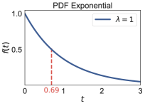
(a)

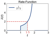
(b)

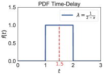
(c)

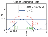
(d)

Figure 1: (a-c) Sampling event times with a rate function $\frac{\mathds{1}_{t\in[1,2]}}{2-t}$. (a) Generate a random variate from the exponential distribution with rate $\lambda=1$, the sample here is $0.69$. (b) We integrate the rate function until the area is $0.69$, here $t_{n}=1.5$. (c) This is the rate function corresponding to the uniform distribution in $\gamma(t)=\mathds{1}_{t\in[1,2]}$. (d) Sampling $t_{n}$ from a time-varying rate function using an upper-bound of $c=1$, rejection probabilities shown in red.

2.1.2 Sampling Time Delays.

The effective rate $\lambda_{n}(t_{\Delta})$ allows us to sample the time delay $t_{n}$ after which agent $n$ fires, using the inversion method. First, we sample an exponential random variate $x$ with rate $1$, then we integrate $\lambda_{n}(t_{\Delta})$ to find $t_{n}$ such that

$$\int_{0}^{t_{n}}\lambda_{n}(t_{\Delta})dt_{\Delta}=x\;.$$ (2)

In general it is possible to pre-compute the integral [28], but its parameterization (on states, residence times, etc) renders this difficult.

Another viable approach is to use rejection sampling. Assume that we have $c\in\mathbb{R}_{\geq 0}$ such that $\lambda_{n}(t_{\Delta})\leq c$ for all $t_{\Delta}$. We start with $t_{n}=0$. In each step, we sample an exponentially distributed random variate $t_{n}^{\prime}$ with rate $c$ and set $t_{n}=t_{n}+t_{n}^{\prime}$. We accept $t_{n}$ with probability $\frac{\lambda_{n}(t_{n})}{c}$. Otherwise we reject it and repeat the process. If a reasonable over-approximation can be constructed, this is typically much faster than the integral approach in (2).

2.1.3 Naïve Simulation Algorithm.

The following simulation algorithm generates statistically correct trajectories of the model. It starts by initializing the global clock $t_{global}=0$ and setting $R(n)=0$ for all $n$. The algorithm repeatedly performs simulation steps until a predefined time horizon or some other stopping criterion is reached. Each stimulation step is as follows:

1. Generate a random time delay (candidate) $t_{n}$ for each agent $n$ using $\gamma_{n}$. Identify agent $n^{\prime}$ with the smallest time delay $t_{n^{\prime}}$.

2. Pick the next state $s^{\prime}$ for $n^{\prime}$ according to $\psi_{n^{\prime}}\big{(}S(n^{\prime}),R(n^{\prime})+t_{n^{\prime}},M(n^{\prime})\big{)}$ and set $S(n^{\prime})=s^{\prime}$. Set $R(n^{\prime})=0$ and $R(n)=R(n)+t_{n^{\prime}}$ ($\forall n\neq n^{\prime}$).

3. Set $t_{global}=t_{global}+t_{n^{\prime}}$ to update the global clock and go to Line 1.

Note that this algorithm is very inefficient as it requires an expensive iteration over all agents and sampling of time delays in each step.

3 Previous Simulation Approaches

Most recent work on non-Markovian dynamics focuses on the mathematical modeling of such processes [29, 30, 31, 32, 33]. In particular, research has focused on how specific distributions (e.g. constant recovery times) alter the properties of epidemic spreading such as the epidemic threshold (see [3, 4] for an overview). However, only few approaches are known for the simulation of non-Markovian dynamics [23, 14]. We shortly review them in the sequel.

3.1 Non-Markovian Gillespie Algorithm

Boguná et al. propose a direct generalization of the Gillespie algorithm to non-Markovian systems, nMGA, which is statistically exact but computationally expensive [23]. The algorithm is conceptually similar to our baseline in Section 2.1 but computes the time delay using so-called survival functions. An agent’s survival function determines the probability that its time delay is larger than a certain time $t_{\Delta}$. The joint survival function of all agents determines the probability that all time delays are larger than $t_{\Delta}$ which can be used to sample the next event time.

The drawback of the nMGA is that it is necessary to iterate over all agents in each step in order to construct their joint survival function. As a fast approximation, the authors suggest to only use the current instantaneous rate at $t=0$ (i.e., $\lambda_{n}(0)$) and assume all rates remain constant until the next event. This is correct in the limit of infinite agents, because when the number of agent approaches infinity, the time until the next firing of any agent approaches zero.

3.2 Laplace-Gillespie Algorithm

The LGA, introduced by Masuda and Rocha in [14], aims at reducing the computational cost of finding the next event time compared to nMGA, while remaining statistically correct. It assumes that the time delay distributions can be expressed in the form of a weighted average of exponential distributions

$$\gamma_{n}(t_{\Delta})=\int_{0}^{\infty}p_{n}(\lambda)\lambda e^{-\lambda t_{\Delta}}d\lambda\;,$$

where $p_{n}$ is a PDF over the rate $\lambda\in\mathbb{R}_{\geq 0}$. This formulation of $\gamma_{n}$, while being very elegant, limits the applicability to cases where the corresponding survival function is completely monotone [14], which limits the set of possible inter-event time distributions.

The LGA has two advantages. Firstly, we can sample $t_{n}$ by first sampling $\lambda$ according to $p_{n}$ and then, instead of the numerical integration in Eq. (2), compute $t_{n}=-\ln u/\lambda$ where $u$ is uniformly distributed on $(0,1)$. Secondly, we can assume that the sampled $\lambda$ for a particular agent remains constant until one of its neighbors fires. Thus, in each step, it is only necessary to update the rates of the neighbors of the firing agent, and not of all agents.

4 Our Method

Rejection sampling for the efficient simulation of Markovian stochastic processes on complex networks has been proposed recently [24, 25, 26, 34], but not for the non-Markovian case where arbitrary distributions for the inter-event times are considered.

Here, we proposes the RED-Sim algorithm for the generation of statistically correct simulations of non-Markovian network models, as described in Section 2. The main idea of RED-Sim is to rely on rejection sampling to reduce the computational cost, making it unnecessary to update the rates of the neighbors of a firing agent. Independently from that, rejection sampling can also be utilized to sample $t_{n}$ without numerical integration.

4.1 Rate Over-Approximation

Recall that $\lambda_{n}(\cdot)$ expresses how the instantaneous rate of $n$ changes over time, assuming that no neighboring agent changes its state. A key in ingredient of our method is now $\widehat{\lambda}_{n}(\cdot)$ which upper-bounds the instantaneous rate of $n$, assuming that all neighbors are allowed to freely change their state as often as possible. That is, at all times $\widehat{\lambda}_{n}(t_{\Delta})$ is an upper-bound of $\lambda_{n}(t_{\Delta})$ taking into consideration all possible states of the neighborhood.

Consider again the Markovian SIS example. The curing of an infected node does not depend on an agent’s neighborhood anyway. The rate is always $c_{r}$, which is a trivial upper bound. A susceptible node becomes infected with rate $c_{i}$ times number of infected neighbors. Thus, the instantaneous infection rate of an agent $n$ can be bounded by $\widehat{\lambda}_{n}(t_{\Delta})=k_{n}c_{i}$ where $k_{n}$ is the degree of $n$. Upper-bounds may also be constant or depend on time. Consider for example a recovery time that is uniformly distributed on $[1,2]$. In this case, $\lambda_{n}(\cdot)$ approaches infinity (cf. Fig. 1b) making a constant upper-bound impossible. For multi-agent models, a time-dependent upper-bound always exists since we can compute the maximal instantaneous rate w.r.t. all reachable neighborhood states.

4.2 The RED-Sim Algorithm

For a given multi-agent model specification $(\mathcal{G},\mathcal{S},\{\phi_{n}\},\{\psi_{n}\},S_{0})$ and given upper-bounds $\{\widehat{\lambda}_{n}\}$, we propose a statistically exact simulation algorithm, which is based on two basic data structures:

Labeled Graph

A graph represents the contact network and each agent (node) $n$ is annotated with its current state $S(n)$ and $T(n)$, the time point of its last state change.

Event Queue

The event queue stores the list of future events, where an event is a tuple $(n,\widehat{\mu},\widehat{t}_{n})$. Here, $n$ is the agent that fires, $\widehat{t}_{n}$ the prospective absolute time point of firing, and $\widehat{\mu}\in\mathbb{R}_{\geq 0}$ is an over-approximation of the true effective rate (at time point $\widehat{t}_{n}$). The queue is sorted w.r.t. $\widehat{t}_{n}$ and initialized by generating one event per agent.

A global clock, $t_{\text{global}}$, keeps track of the elapsed time since the simulation started. We use $T(n)$ instead of $R(n)$ to avoid updates for all agents after each event (i.e., $R(n)=t_{\text{global}}-T(n)$). We perform simulation steps until some termination criterion is fulfilled, each step is as follows:

1. Take the first event $(n,\widehat{\mu},\widehat{t}_{n})$ from the event queue and update $t_{\text{global}}=\widehat{t}_{n}$.

2. Evaluate the true instantaneous rate $\mu=\phi_{n}\big{(}S(n),t_{\text{global}}-T(n),M(n)\big{)}$ of $n$ at the current system state.

3. With probability $1-\frac{\mu}{\widehat{\mu}}$, reject the firing and go to Line 5.

4. Randomly choose the next state $s^{\prime}$ of $n$ according to the distribution
   $\psi_{n}\big{(}S(n),t_{\text{global}}-T(n),M(n)\big{)}$. If $S(n)\neq s^{\prime}$: set $S(n)=s^{\prime}$ and $T(n)=t_{\text{global}}$.

5. Generate a new event for agent $n$ and push it to the event queue.

6. Go to Line 1.

The correctness of RED-Sim can be shown similarly to [26, 24] (see also the proof sketch in Appendix A). Note that in all approaches evaluating an agent’s instantaneous rate is linear in the number of its neighbors. In previous approaches, the rate has to be updated for all neighbors of a firing agent. In RED-Sim only the rate of the firing agent has to be updated. The key asset of RED-Sim is that, due to the over-approximation of the rate function, we do not need to update the neighborhood of the firing agent $n$, even though the neighbor’s respective rates might change as a result from the event. We provide a more detailed analysis of the time-complexity of RED-Sim in Appendix B.

4.2.1 Event Generation.

To generate new events in Line 5, we sample a random time delay $t_{n}$ and set $\widehat{t}_{n}=t_{\text{global}}+t_{n}$. To sample $t_{n}$ according to the over-approximated rate $\widehat{\lambda}_{n}(\cdot)$, we either use the integration approach of Eq. (2) or sample directly from an upper-bounded the exponential distribution (cf. Fig. 1d).

To sample $t_{n}$ from an exponential distribution, we need to be able to find an upper bound that is constant in time $\widehat{\lambda}_{n}(t)=c$ for all $t$. Hence, we simply set $\widehat{\mu}=c$ and sample $t_{n}$ from an exponential distribution with rate $c$. Otherwise, when a constant upper bound either does not exits or is unfeasible to construct, we use numerical integration over $\widehat{\lambda}_{n}(\cdot)$ (see Eq. (2)), and set $\widehat{\mu}=\widehat{\lambda}_{n}(t_{n})$. Alternatively, when $\widehat{\lambda}_{n}(t)$ has the required form (cf. Section 3), we can even use LGA-like approach to sample $t_{n}$ [23] (and also set $\widehat{\mu}=\widehat{\lambda}_{n}(t_{n})$).

4.2.2 Discussion.

We expect RED-Sim to perform poor only in some special cases, where either the construction of an upper-bound is numerically too expensive or where the difference between the upper-bound and the actual average rate is very large, which would render the number of rejections events too high.

It is easy to extend RED-Sim to different types of non-Markovian behavior. For instance, we might keep track of the number of firings of an agent and parameterize $\phi$ and $\psi$ accordingly to generate the behavior of self-exiting point processes or to cause correlated firings among agents [36, 37].

Note that, we can turn the method into a rejection-free approach by generating a new event for $n$ and all of its neighbors in Line 5 while taking the new state of $n$ into consideration (see also Appendix A).

5 Case Studies

We demonstrate the effectiveness our approach on classical epidemic-type processes and synthetically generated networks following the configuration model with a truncated power-law degree distribution [38]. That is $P(k)\propto k^{-\beta}$ for $3\leq k\leq|\mathcal{N}|$. We use $\beta\in\{2,2.5\}$ (a smaller $\beta$ corresponds to a larger average degree). The implementation is written in Julia and publicly available. As a baseline for comparison, we use the rejection-free variant of the algorithm where neighbors are updated after an event (as described at the end of Section 4.2). The evaluation was performed on a 2017 MacBook Pro with a 3.1 GHz Intel Core i5 CPU and results are shown in Fig. 2.

5.0.1 SIS Model.

We consider an SIS model (with $\psi$ and $\phi$ as defined above), but infected nodes become less infectious over time. That is, the rate at which an infected agent with residence time $t$ attacks its susceptible neighbors is $ue^{-ut}$ for $u=0.4$. This shifts the exponential distribution to the left. We upper-bound the infection rate of an agent $n$ with degree $k_{n}$ with $\widehat{\lambda}_{n}(t)=uk_{n}$ which is constant in time. Thus, we sample $t_{n}$ using an exponential distribution. The time until an infected agent recovers is, independent from its neighborhood, uniformly distributed in $[0,1]$ (similar to [39]). Hence, we can sample it directly. We start with $5\%$ infected agents.

5.0.2 Voter Model.

The voter model describes the competition of two opinions of agents in state A switch to B and vice versa (i.e. $\psi$ is deterministic). The time until an agent switches follows a Weibull distribution (similar to [23, 40]):

$$\gamma_{n}(t)=cu(tu)^{c-1}e^{-{(tu)}^{c}}\hskip 14.22636pt\text{and}\hskip 14.22636pt\lambda_{n}(t)=cu(tu)^{c-1},\;t\geq 0$$

where we set $c=c_{A}=2.0$, $u=u_{A}$ if $S(n)=\texttt{A}$ and $c=c_{B}=2.05$, $u=u_{B}$ if $S(n)=\texttt{B}$. We let the fraction of opposing neighbors modulate $u$, i.e., $u_{A}=\frac{B_{n}}{k_{n}}$, where $B_{n}$ denotes the number of neighbors currently in state B and $k_{n}$ is the degree of agent $n$ (and analogously for A). Hence, the instantaneous rate depends on the current residence time and the states of the neighboring agents. To get an upper-bound for the rate, we set $u_{A}=u_{B}=1$ and get $\widehat{\lambda}_{n}(t)=ct^{c-1}$. We use numerical integration to sample $t_{n}$ to show that RED-Sim performs well also in the case of this more costly sampling. We start with $50\%$ of agents being in each state.

5.0.3 Discussion.

Our results provide strong evidence for the usefulness of rejection sampling for non-Markovian simulation. As expected, we find that the number of interconnections (edges) and the number of agents influence the runtime behavior. Especially for RED-Sim, the number of edges shows to be much more relevant than purely the number of agents. Our method consistently outperforms the baseline up to several orders of magnitude. The gain (RED-Sim speed by baseline speed) ranges from $10.2$ ($10^{3}$ nodes, voter model, $\beta=2.5$) to $674$ ($10^{5}$ nodes, SIS model, $\beta=2.0$).

We expect the baseline algorithm to be comparable with LGA as both of them only update the rates of the relevant agents after an event. Moreover, in the SIS model, sampling the next event times is very cheap. However, a detailed statistical comparison remains to be performed (both case-studies could not straightforwardly be simulated with LGA due to its constraints on the time delays). Note that, when LGA is applicable, its key asset, the fast sampling of time delays, can also be used in RED-Sim. We also tested a nMGA-like implementation where rates are consider to remain constant until the next event. However, the method was—even though it is only approximate—slower than the baseline.

Note that the SIS model is somewhat unfavorable for RED-Sim as it generates a large amount of rejection events when only a small fraction of agents are infected. Consider, for instance, an agent with many neighbours of which only a few are infected. The over-approximation essentially assumes that all neighbors are infected to sample the next event time (and, in addition, over-approximates the rate of each individual neighbor), leading to a high rejection probability. Nevertheless, the low computational costs of each rejection event overcome this.

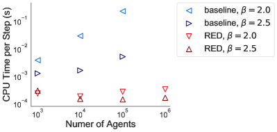
(a)

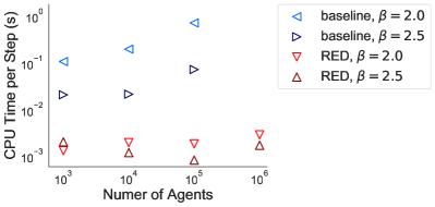
(b)

Figure 2: Computation time of a single simulation step w.r.t. network size and connectivity of the SIS model (a) and voter model (b). We measure the CPU time per simulating step by dividing the simulation time by the number of successful (i.e., non-rejection) steps.

6 Conclusions

We presented a rejection-based algorithm for the simulation of non-Markovian agent models on networks. The key advantage of the rejection-based approach is that in each simulation step it is no longer necessary to update the rates of neighboring agents. This greatly reduces the time complexity of each step compared to previous approaches and makes our method viable for the simulation of dynamical processes on real-world networks. As future work, we plan to automate the computation of the over-approximation $\widehat{\lambda}$ and investigate correlated time delays [41, 14] and self-exiting point processes [36, 37].

6.0.1 Acknowledgements.

We thank Guillaume St-Onge for helpful comments on non-Markovian dynamics. This research was been partially funded by the German Research Council (DFG) as part of the Collaborative Research Center Methods and Tools for Understanding and Controlling Privacy.

Appendix A Correctness

First, consider the rejection-free version of the algorithm:

1. Take the first event $(n,\widehat{\mu},\widehat{t}_{n})$ from the event queue and update $t_{\text{global}}=\widehat{t}_{n}$.

2. Evaluate the true instantaneous rate $\mu=\phi_{n}\big{(}S(n),t_{\text{global}}-T(n),M(n)\big{)}$ of $n$ at the current system state.

3. With probability $1-\frac{\mu}{\widehat{\mu}}$, reject the firing and go to Line 5.

4. Randomly choose the next state $s^{\prime}$ of $n$ according to the distribution
   $\psi_{n}\big{(}S(n),t_{\text{global}}-T(n),M(n)\big{)}$. If $S(n)\neq s^{\prime}$: set $S(n)=s^{\prime}$ and $T(n)=t_{\text{global}}$.

5. Generate a new event for agent $n$ and push it to the event queue.

6. For each neighbor $n^{\prime}$ of $n$: Remove the event corresponding to $n^{\prime}$ from the queue and generate a new event (taking the new state of $n$ into account).

7. Go to Line 1.

Rejection events are not necessary in this version of the algorithm because all events in the queue are generated by the real rate and are therefore consistent with the current system state. It is easy to see that the rejection-free version is a direct event-driven implementation of the Naïve Simulation Algorithm which specifies the semantics in Section 2.1.3. The correspondence between Gillespie-approaches and even-driven simulation exploited in literature, for instance in [4]. Thus, it is sufficient to show that the rejection-free version and RED-Sim (Section 4.2) are statistically equivalent.

We do this with the following trick: We modify $\phi_{n}$ and $\psi_{n}$ into $\widehat{\phi}_{n}$ and $\widehat{\psi}_{n}$, respectively. When we simulate the rejection-free algorithm, it will admit exactly the same behavior as RED-Sim. The key to that are so-called shadow-process [24, 26]. A shadow process does not change the state of the corresponding agent but still fires with a certain rate. They are conceptually similar to self-loops in a Markov chain. In the end, we can interpret the rejection events not as rejections, but as the statistically necessary application of the shadow process.

Here, we consider the case where a constant upper-bound $c\in\mathbb{R}_{\geq 0}$ exits for all $\phi_{n}$. That is, $c\geq\phi_{n}(s,t,m)$ for all reachable $s,t,m$. The case of an time-dependent upper-bound is, however, analogous. Now, for each $n$, we define the shadow-process $\tilde{\phi}_{n}$ as

$$\widetilde{\phi}_{n}(s,t,m)=c-\phi_{n}(s,t,m)\;.$$

Consequently, for all $n,s,t,m$:

$$\widehat{\phi}_{n}(s,t,m)=c=\phi_{n}(s,t,m)+\widetilde{\phi}_{n}(s,t,m)$$

The only thing remaining is to define $\widehat{\phi}_{n}$ such that the shadow-process really has no influence on the system state. Therefore, we simply trigger a null event (or self-loop) with the probability proportional to how much of $\widehat{\phi}_{n}$ is induced by the shadow-process. Formally,

$$\widehat{\psi}_{n}(s,t,m)=\begin{cases}p(s)=1\text{\;\;\;\;\;\;(self-loop) with probability\;\;}\frac{\widetilde{\phi}_{n}}{\widehat{\phi}_{n}}\\ \psi_{n}(s,t,m)\text{\hskip 49.79231pt otherwise}\end{cases}.$$

Note that, firstly, the model specification with $\widehat{\phi}_{n},\widehat{\psi}_{n}$ or ${\phi}_{n},{\psi}_{n}$ are equivalent, because $\widetilde{\phi},\widetilde{\psi}$ has to actual effect on the system. Secondly, simulating the rejection-free algorithm with $\widehat{\phi}_{n},\widehat{\psi}_{n}$ directly yields RED-Sim. In particular, the rejections events have the same likelihood as the shadow-process being chosen in $\widehat{\psi}$. Moreover, updating the rates of all neighbors is redundant because all the rates remain at $c$. Whatever the change in $\phi_{n}$ is, after an event, that shadow process balances it out, such hat it actually remains constant.

For the case that an upper-bound $c$ does not exits, we can still look at the limit case of $c\rightarrow\infty$. In particular, we truncate all rate functions at $c$ and find that, as $c$ approaches infinity, the simulated model approaches the real model.

Appendix B Time-Complexity

Next, we discuss how the runtime of RED-Sim scales with the size of the underlying contact network (and number of agents). Assume that a binary heap is used to implement the event queue and that the graph structure is implemented using a hashmap. Each step starts by popping an element from the queue which has constant time complexity. Next, we compute $\mu$. Therefore, we have to lookup all neighbors of $n$ in the graph structure iterate over them. We also have to lookup all states and residence times. This step has linear time-complexity in the number of neighbors. More precisely, lookups in the hashmaps have constant time-complexity on average and are linear in the number of agents in the worst case. Computing the rejection probability has constant time complexity. In the case of a real event, we update $S$ and $T$. Again, this has constant time-complexity on average. Generating a new event does not depend on the neighborhood of an agent and has, therefore, constant time-complexity. Note that this step can still be somewhat expensive when it requires integration to sample $t_{e}$ but not in an asymptotic sense. Thus, a step in the simulation is linear in the number of neighbors of the agent under consideration.

In contrast, previous methods require that after each update, the rate of each neighbor $n^{\prime}$ is re-computed. The rate of $n^{\prime}$, however, depends on the whole neighborhood of $n^{\prime}$. Hence, it is necessary to iterate over all neighbors $n^{\prime\prime}$ of every single neighbor $n^{\prime}$ of $n$.

References

- [1] Albert-László Barabási. Network science. Cambridge university press, 2016.
- [2] John Goutsias and Garrett Jenkinson. Markovian dynamics on complex reaction networks. Physics Reports, 529(2):199–264, 2013.
- [3] Romualdo Pastor-Satorras, Claudio Castellano, Piet Van Mieghem, and Alessandro Vespignani. Epidemic processes in complex networks. Reviews of modern physics, 87(3):925, 2015.
- [4] István .Z Kiss, J. C Miller, and P. L Simon. Mathematics of epidemics on networks. Forthcoming in Springer TAM series, 2016.
- [5] Mason Porter and James Gleeson. Dynamical systems on networks: A tutorial, volume 4. Springer, 2016.
- [6] Helena Sofia Rodrigues. Application of sir epidemiological model: new trends. arXiv preprint arXiv:1611.02565, 2016.
- [7] Maksim Kitsak, Lazaros K Gallos, Shlomo Havlin, Fredrik Liljeros, Lev Muchnik, H Eugene Stanley, and Hernán A Makse. Identification of influential spreaders in complex networks. Nature physics, 6(11):888, 2010.
- [8] Laijun Zhao, Jiajia Wang, Yucheng Chen, Qin Wang, Jingjing Cheng, and Hongxin Cui. Sihr rumor spreading model in social networks. Physica A: Statistical Mechanics and its Applications, 391(7):2444–2453, 2012.
- [9] AV Goltsev, FV De Abreu, SN Dorogovtsev, and JFF Mendes. Stochastic cellular automata model of neural networks. Physical Review E, 81(6):061921, 2010.
- [10] Jil Meier, X Zhou, Arjan Hillebrand, Prejaas Tewarie, Cornelis J Stam, and Piet Van Mieghem. The epidemic spreading model and the direction of information flow in brain networks. NeuroImage, 152:639–646, 2017.
- [11] Chenquan Gan, Xiaofan Yang, Wanping Liu, Qingyi Zhu, and Xulong Zhang. Propagation of computer virus under human intervention: a dynamical model. Discrete Dynamics in Nature and Society, 2012, 2012.
- [12] Robert M May and Nimalan Arinaminpathy. Systemic risk: the dynamics of model banking systems. Journal of the Royal Society Interface, 7(46):823–838, 2009.
- [13] Robert Peckham. Contagion: epidemiological models and financial crises. Journal of Public Health, 36(1):13–17, 2013.
- [14] Naoki Masuda and Luis EC Rocha. A gillespie algorithm for non-markovian stochastic processes. SIAM Review, 60(1):95–115, 2018.
- [15] Alun L Lloyd. Realistic distributions of infectious periods in epidemic models: changing patterns of persistence and dynamics. Theoretical population biology, 60(1):59–71, 2001.
- [16] GL Yang. Empirical study of a non-markovian epidemic model. Mathematical Biosciences, 14(1-2):65–84, 1972.
- [17] SP Blythe and RM Anderson. Variable infectiousness in hfv transmission models. Mathematical Medicine and Biology: A Journal of the IMA, 5(3):181–200, 1988.
- [18] T D. Hollingsworth, R. M Anderson, and C. Fraser. Hiv-1 transmission, by stage of infection. The Journal of infectious diseases, 198(5):687–693, 2008.
- [19] Z Feng and HR Thieme. Endemic models for the spread of infectious diseases with arbitrarily distributed disease stages i: General theory. SIAM J. Appl. Math, 61(3):803–833, 2000.
- [20] Albert-Laszlo Barabasi. The origin of bursts and heavy tails in human dynamics. Nature, 435(7039):207, 2005.
- [21] Alexei Vázquez, Joao Gama Oliveira, Zoltán Dezsö, Kwang-Il Goh, Imre Kondor, and Albert-László Barabási. Modeling bursts and heavy tails in human dynamics. Physical Review E, 73(3):036127, 2006.
- [22] William R Softky and Christof Koch. The highly irregular firing of cortical cells is inconsistent with temporal integration of random epsps. Journal of Neuroscience, 13(1):334–350, 1993.
- [23] Marian Boguná, Luis F Lafuerza, Raúl Toral, and M Ángeles Serrano. Simulating non-markovian stochastic processes. Physical Review E, 90(4):042108, 2014.
- [24] Wesley Cota and Silvio C Ferreira. Optimized gillespie algorithms for the simulation of markovian epidemic processes on large and heterogeneous networks. Computer Physics Communications, 219:303–312, 2017.
- [25] Guillaume St-Onge, Jean-Gabriel Young, Laurent Hébert-Dufresne, and Louis J Dubé. Efficient sampling of spreading processes on complex networks using a composition and rejection algorithm. arXiv preprint arXiv:1808.05859, 2018.
- [26] Gerrit Großmann and Verena Wolf. Rejection-based simulation of stochastic spreading processes on complex networks. In International Workshop on Hybrid Systems Biology, pages 63–79. Springer, 2019.
- [27] David Roxbee Cox. Renewal theory. 1962.
- [28] Raghu Pasupathy. Generating homogeneous poisson processes. Wiley encyclopedia of operations research and management science, 2010.
- [29] I. Z Kiss, G. Röst, and Z. Vizi. Generalization of pairwise models to non-markovian epidemics on networks. Physical review letters, 115(7):078701, 2015.
- [30] Lorenzo Pellis, Thomas House, and Matt J Keeling. Exact and approximate moment closures for non-markovian network epidemics. Journal of theoretical biology, 382:160–177, 2015.
- [31] Hang-Hyun Jo, Juan I Perotti, Kimmo Kaski, and János Kertész. Analytically solvable model of spreading dynamics with non-poissonian processes. Physical Review X, 4(1):011041, 2014.
- [32] N Sherborne, JC Miller, KB Blyuss, and IZ Kiss. Mean-field models for non-markovian epidemics on networks: from edge-based compartmental to pairwise models. arXiv preprint arXiv:1611.04030, 2016.
- [33] Michele Starnini, James P Gleeson, and Marián Boguñá. Equivalence between non-markovian and markovian dynamics in epidemic spreading processes. Physical review letters, 118(12):128301, 2017.
- [34] C. L Vestergaard and M. Génois. Temporal gillespie algorithm: Fast simulation of contagion processes on time-varying networks. PLoS computational biology, 11(10):e1004579, 2015.
- [35] Gerrit Großmann, Luca Bortolussi, and Verena Wolf. Rejection-based simulation of non-markovian agents on complex networks. arXiv preprint arXiv:2878114, 2016.
- [36] Yosihiko Ogata. On lewis’ simulation method for point processes. IEEE Transactions on Information Theory, 27(1):23–31, 1981.
- [37] Angelos Dassios, Hongbiao Zhao, et al. Exact simulation of hawkes process with exponentially decaying intensity. Electronic Communications, 18, 2013.
- [38] B K Fosdick, D B Larremore, J Nishimura, and J Ugander. Configuring random graph models with fixed degree sequences. SIAM Review, 60(2):315–355, 2018.
- [39] Gergely Röst, Zsolt Vizi, and István Z Kiss. Impact of non-markovian recovery on network epidemics. In BIOMAT 2015: International Symposium on Mathematical and Computational Biology, pages 40–53. World Scientific, 2016.
- [40] P Van Mieghem and R Van de Bovenkamp. Non-markovian infection spread dramatically alters the susceptible-infected-susceptible epidemic threshold in networks. Physical review letters, 110(10):108701, 2013.
- [41] Hang-Hyun Jo, Byoung-Hwa Lee, Takayuki Hiraoka, and Woo-Sung Jung. Copula-based algorithm for generating bursty time series. arXiv preprint arXiv:1904.08795, 2019.