Transmission of waves across atomic step discontinuities in discrete nanoribbon structures

Abstract

Scalar wave propagation across a semi-infinite step or step-like discontinuity on any one boundary of the square lattice waveguides is considered within nearest-neighbour interaction approximation. An application of the Wiener–Hopf method does yield an exact solution of the discrete scattering problem, using which, as the main result of the paper, the transmission coefficients for energy flux are obtained. It is assumed that a wave mode is incident from either side of the step and the question addressed is what fraction of incident energy is transmitted across the atomic step discontinuity. A total of ten configurations are presented that arise due to various placements of discrete Dirichlet and Neumann boundary conditions on the waveguide. Numerical illustrations of a measure of ‘conductance’ are provided.

Introduction

Historically, an understanding of the surface roughness induced scattering of waves has played a crucial role in the subject of mechanics, physics, and thermodynamics of solids [Papadopoulos1957, Cahill1, Cahill2, Fellay, Ladik1987, Kosevich2008, Kosevichmulti, santamore2001effect, sanchez1998coexistence, sanchez1999reflection, Mujica1994_1, Virlouvet]. Classically, research works on waveguides, with scattering due to steps, have been carried out by numerous investigators due to their importance in elastic, acoustic, and electromagnetic wave propagation theory; some of the results are also obtained through the Wiener–Hopf technique [Wiener, Noble, mittra1971analytical]. On the other hand, the discrete models appear in many applications involving crystalline matter with or without impurities [kosevich], thin films or monolayers [Ohring2002711, Gong, Ohtake], etc. Within this context of surface induced phenomena, the present paper extends the applications of recent framework developed for discrete scattering problems [Bls0, Bls1, Bls8pair1]. In contrast to the recent investigation of the wave transmission of surface localized anti-plane shear wave [Victor_Bls_surf2] in lattice structures, motivated by certain discrete counterpart [Victor_Bls_surf1] of Gurtin-Murdoch model [GurtinMurdoch1975a, gurtin1978surface, steigmann1997plane, SteigmannOgden1999], the present paper applies similar methodology to reveal the transmission characteristic associated with a close-up of discrete form of surface roughness.

As observed in this paper, the time harmonic response of lattice waveguides, modulo the presence of a step or a step-like discontinuity, is also remarkable. It turns out that there exist frequency intervals where certain measure of conductance [Rego1998, schwab2000measurement]) is large and in some other intervals there is dominant effect of step induced scattering, depending on the boundary conditions as well. It can be envisaged that the techniques and results of the paper assume qualitative relevance to more complex physical systems [marcuvitz1951waveguide, collin1991field, linton2001handbook, BurnsMilton, kokubo2011waveguide]. The lattice waveguides also demonstrate a quasi-one dimensional character, providing a pathway to venture into the effect of second dimension in physical space. The paper maintains focus on the effects due to presence of confinement, incorporated by the boundary conditions. The derived results which can be obtained, more or less directly, based on the manipulations and expressions of the exact solution on infinite square lattice [Bls0, Bls1] and lattice waveguides [Bls9s], have been omitted in the main paper. Throughout the paper, a useful role is played by Chebyshev polynomials [MasonHand].

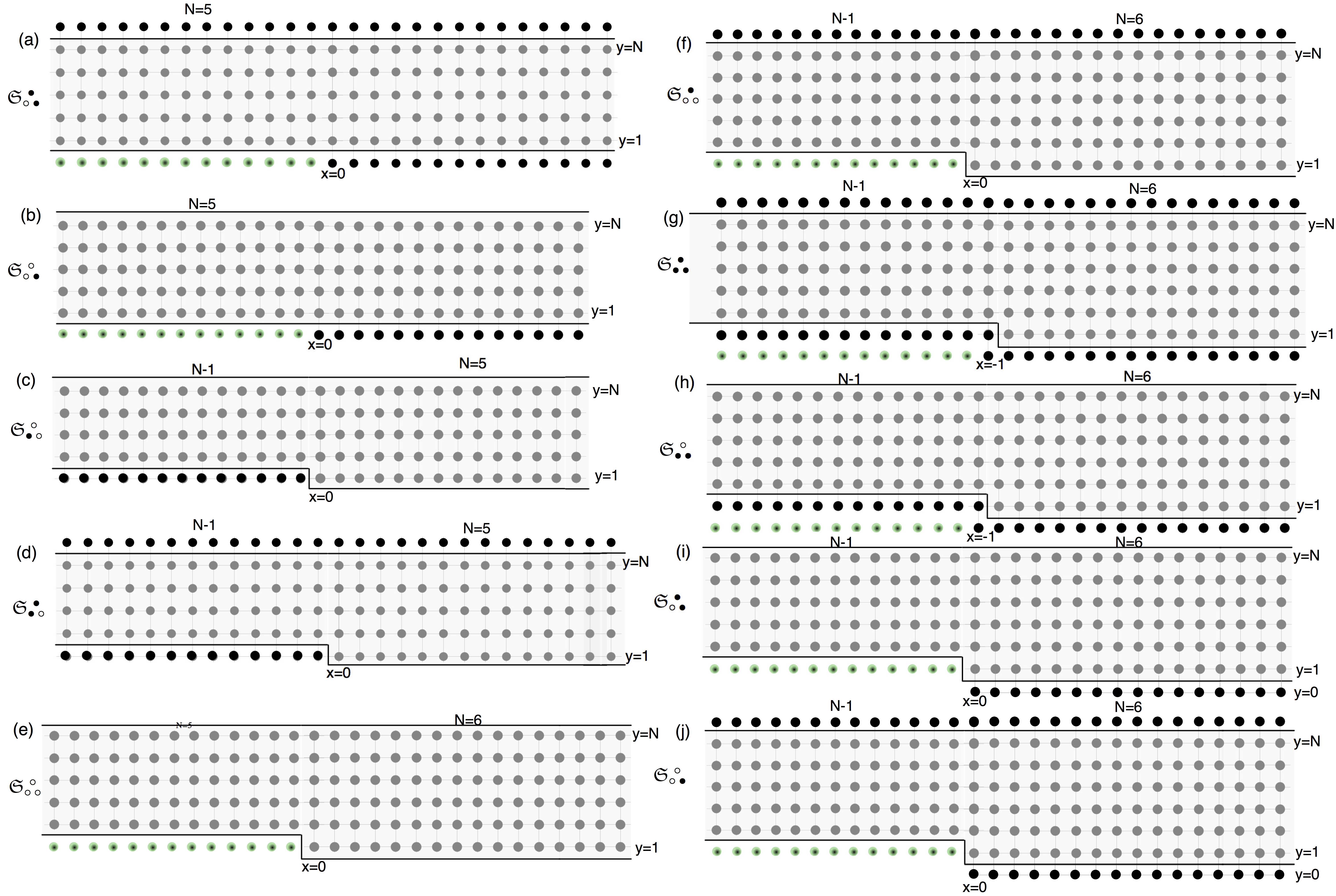
Figure 1: Waveguides of square lattice structure with step-like (a–d) discontinuity induced by a union of semi-infinite ‘discrete Neumann’ and ‘discrete Dirichlet’ (a, b) boundary and a semi-infinite ‘discrete Dirichlet’ and ‘discrete Neumann’ (c, d) boundary or a step (e–h) discontinuity on a ‘discrete Neumann’ (e, f) and a ‘discrete Dirichlet’ (g, h) boundary.

1 Square lattice waveguide

Consider a strip with ${\mathtt{N}}$ number of rows of the square lattice structure, $\{\nu^{i}\hat{\mathbf{{e}}}_{i}\big{|}\nu^{1}\in{\mathbb{Z}},\nu^{2}\in\mathbb{Z}_{1}^{{\mathtt{N}}}\}.$ Each particle of such discrete nanoribbon structure is assumed to possess unit mass, and, interaction with atmost its four nearest neighbours through linearly elastic identical (massless) bonds with a spring constant $1/\mathrm{b}^{2}$. The notation follows that introduced for an infinite lattice [Bls0, Bls1] and the square lattice waveguides [Bls9, Bls9s]. Due to nature of the problem, the displacement of a particle, located at the site indexed by its lattice coordinates $({\mathtt{x}},{\mathtt{y}})\in{{\mathbb{Z}^{2}}}$ in ${\mathfrak{S}}_{{\mathtt{N}}}$ and denoted by ${\mathtt{u}}_{{\mathtt{x}},{\mathtt{y}}}$, is complex valued. The equation of motion of the particles in ${\mathfrak{S}}_{{\mathtt{N}}}$ away from the upper and lower boundaries is b^2¨u_x, y&=△u_x, y, where △u_x, y:=u_x+1, y+u_x-1, y+u_x, y+1+u_x, y-1-4u_x, y. The equation of motion at upper (corresponding to “$-$”) and (each left or right part of the) lower (corresponding to “$+$”) boundary rows studied in this paper is either

$$\mathrm{b}^{2}\ddot{\mathtt{u}}_{{{\mathtt{x}}},{{\mathtt{y}}}} ={\mathtt{u}}_{{{\mathtt{x}}}+1,{{\mathtt{y}}}}+{\mathtt{u}}_{{{\mathtt{x}}}-1,{{\mathtt{y}}}}+{\mathtt{u}}_{{{\mathtt{x}}},{{\mathtt{y}}}\mp 1}-4{\mathtt{u}}_{{{\mathtt{x}}},{{\mathtt{y}}}} {\bullet}$$ () (1.1a)

$$\text{or }\mathrm{b}^{2}\ddot{\mathtt{u}}_{{{\mathtt{x}}},{{\mathtt{y}}}} ={\mathtt{u}}_{{{\mathtt{x}}}+1,{{\mathtt{y}}}}+{\mathtt{u}}_{{{\mathtt{x}}}-1,{{\mathtt{y}}}}+{\mathtt{u}}_{{{\mathtt{x}}},{{\mathtt{y}}}\mp 1}-3{\mathtt{u}}_{{{\mathtt{x}}},{{\mathtt{y}}}} \text{(${\circ}$)}.$$ (1.1b)

In the context of the waveguides with step (or step-like) discontinuity studied in this paper, in particular, on the upper free boundary (resp. on row adjacent to fixed boundary) (1.1b) holds (resp. (1.1a)) with $-$ sign; on the lower free boundary (resp. on row adjacent to fixed boundary) (1.1b) holds (resp. (1.1a)) for ${\mathtt{x}}<0$ and/or ${\mathtt{x}}\geq 0$ with $+$ sign. The same geometric structure can be also interpreted as a junction of two semi-infinite waveguides of either of the four kinds as stated in [Bls9] (briefly recalled in Appendix LABEL:app_recallbifwavesq_Chebdef). The ten configurations shown in Fig. 1 as a graphical schematic illustration of the boundary conditions. Again the notation is self-explanatory as the superscript on ${\mathfrak{S}}$ represents the upper boundary condition and the subscript represents the pair of two semi-infinite lower boundary conditions. Fig. 1 illustrates schematically the step discontinuity induced by a union of semi-infinite ‘discrete Neumann’ and ‘discrete Dirichlet’ (i, j) boundary. The green dots are unconnected hypothetical sites used in mathematical formulation. The sites contained in the shaded region bounded by the solid lines belong to the waveguide, wherein the sites adjacent to the solid lines belong to ${\Sigma}$ (such that (1.1a) or (1.1b) holds).

Suppose ${\mathtt{u}}^{{\text{in}}}$ describes the incident wave mode (indexed by natural number ${{\kappa}}^{{\text{in}}}$ [Bls9]) with frequency $\omega$ and a lattice wave number ${\upkappa}_{x}$ along ${\mathtt{x}}$ coordinate. The ordinary frequency $\omega$ (aside from a factor due to scaling of time [Bls0]) corresponds to a propagating mode lying in the pass band of lattice waveguide either on the left or right side of the step discontinuity. It is assumed that ${\mathtt{u}}^{{\text{in}}}$ is given by an expression of the form u_x, y^in:=Aa_(κ^in)ye^-iκ_x x-iωt, ∀(x, y)∈Z^2N, where ${{\mathrm{A}}}\in\mathbb{C}$ is constant. The symbol ${{a}}_{({{\kappa}}^{{\text{in}}})\cdot}$ represents the mode shape corresponding to the specific wave mode indexed by ${{\kappa}}^{{\text{in}}}$ (see [Bls9] or Appendix C of [Bls9s] for the detailed expressions). In the remaining text, the explicit time dependence factor, $e^{-i\omega t}$, is suppressed.

Let the lattice frequency ${\upomega}$ be defined as ${\upomega}{:=}\mathrm{b}\omega,$ so that ${\upomega}^{2}=4(\sin^{2}{\frac{1}{2}}{\upkappa}_{x}+\sin^{2}{\frac{1}{2}}{\upeta_{\kappa^{\text{in}}}}),{\upkappa}_{x}\in[-\pi,\pi],$ where ${\upeta_{\kappa^{\text{in}}}}$ is interpreted as the vertical component of an incident wave vector in (bulk) lattice. Clearly, ${\upeta_{\kappa^{\text{in}}}}$ depends on the confinement effect of the boundary conditions [Bls9]. The total displacement ${\mathtt{u}}^{{t}}$ of an arbitrary particle in each lattice waveguide is a sum of the incident wave displacement ${\mathtt{u}}^{{\text{in}}}$ and the scattered wave displacement ${\mathtt{u}}^{{s}}$. Henceforth, the letter ${\mathtt{u}}$ is used in place of ${\mathtt{u}}^{{s}}$. The total displacement field ${\mathtt{u}}^{{t}}$ ($={\mathtt{u}}_{{\mathtt{x}},{\mathtt{y}}}^{{\text{in}}}+{\mathtt{u}}_{{\mathtt{x}},{\mathtt{y}}}$) satisfies the discrete Helmholtz equation △u^t_x, y+ω^2u^t_x, y&=0, (x, y)∈Z^2N∖Σ with ω=ω_1+iω_2, ω_2¿0, where ${{\Sigma}}$ is boundary of the waveguide (as enumerated in Fig. 1). The discrete Fourier transform [jury, Slepyanbook] ${\mathtt{u}}_{{\mathtt{y}}}^{F}:\mathbb{C}\to\mathbb{C}$ of $\{{\mathtt{u}}_{{\mathtt{x}},{\mathtt{y}}}\}_{{\mathtt{x}}\in\mathbb{Z}}$ (along the ${\mathtt{x}}$ axis) is defined by u_y^F&=u_y;++u_y;-, where u_y;+(z)=∑_x=0^+∞ u_x, yz^-x, u_y;-(z)=∑_x=-∞^-1 u_x, yz^-x. The discrete Fourier transform ${\mathtt{u}}_{{\mathtt{y}}}^{F}$ of $\{{\mathtt{u}}_{{\mathtt{x}},{\mathtt{y}}}\}_{{\mathtt{x}}\in\mathbb{Z}}$ is well defined for all relevant values of (fixed) ${\mathtt{y}}$ [Bls9s] in an annulus ${\mathscr{A}}$ in the complex plane (same as that defined in [Bls9s], ${{\mathit{R}}}_{\pm}$ are given in Appendix A of [Bls9s], namely, equation (A.1) ${{\mathit{R}}}_{+}=e^{-{\upkappa}_{2}},{{\mathit{R}}}_{-}=e^{+{\upkappa}_{2}}$).

2 Step or step-like discontinuity induced by a semi-infinite fixed or free boundary

In this section the ten wave-guides with boundary containing a step (or step-like discontinuity), as shown schematically in Fig. 1, are considered one by one. It is assumed that the wave is incident from the portion ahead of the step (the other case of incidence is treated afterwards).

2.1 Incidence from the broad portion of the step discontinuity

2.1.1 Case: (a)

In this case the particles at ${\mathtt{x}}\in\mathbb{Z},{\mathtt{y}}={{\mathtt{N}}}+1$ and ${\mathtt{x}}\geq 0,{\mathtt{y}}=0$ are fixed while those at ${\mathtt{x}}<0,{\mathtt{y}}=1$ belong to a free boundary, as shown in Fig. 1(a). Thus, ${\mathfrak{S}}{\mathbin{\begin{subarray}{c}{\bullet}\\ {\circ}{\bullet}\end{subarray}}}$ is the waveguide constructed by a junction between ${\mathfrak{S}{\genfrac{}{}{0.0pt}{1}{\raisebox{-1.50694pt}{$\bullet$}}{\raisebox{1.50694pt}{$\circ$}}}}$ and ${\mathfrak{S}{\genfrac{}{}{0.0pt}{1}{\raisebox{-1.50694pt}{$\bullet$}}{\raisebox{1.50694pt}{$\bullet$}}}}$ of width ${\mathtt{N}}$ (recall the notation described in Appendix LABEL:app_recallbifwavesq_Chebdef or [Bls9]). Using the general solution (1) in the square lattice (LABEL:gensol_sq) and upper boundary condition (1.1a),

$${\mathtt{u}}_{{\mathtt{y}}}^{F}={\mathtt{u}}^{F}_{1}{\Lambda}_{{\mathtt{y}}}({\mathtt{N}},{\bullet};1),{{\mathtt{y}}}\in\mathbb{Z}_{1}^{{\mathtt{N}}},$$ (2.1a)

$$\text{where }{\Lambda}_{{\mathtt{y}}}(n,{\bullet};1)=\frac{{{\lambda}}^{{\mathtt{y}}-1}-{{\lambda}}^{2{n}-{{\mathtt{y}}}+1}}{1-{{\lambda}}^{2{n}}},$$ (2.1b)

where ${\lambda}$ [Slepyanbook, Bls0] is defined by (LABEL:lambdadef_sq) and the variable of these complex functions (${z}$) lies in ${\mathscr{A}}$. According to (2.1a), it is easy to notice that ${\mathtt{u}}_{\cdot,{\mathtt{y}}}$ equals ${\mathtt{u}}_{\cdot,1}$ for ${\mathtt{y}}=1$, and is identically zero for ${\mathtt{y}}={{\mathtt{N}}}+1$ (due to the presence of normal mode factor in (1), ${{\mathtt{u}}^{{\text{in}}}_{\cdot,0}}=0,$ ${{\mathtt{u}}^{{\text{in}}}_{\cdot,{\mathtt{N}}+1}}=0$). As an analogue of (1) for ${\mathtt{y}}=1,$ &(-ω^2u_x, 1-b^2v^t_x)=-(u_x, 0^in-u_x, 1^in) +(u_x+1, 1+u_x-1, 1+u_x, 2-3u_x, 1), where ${{{\mathit{v}}}^{{t}}}_{{\mathtt{x}}}$ is the total force that acts on the particle $({{\mathtt{x}}},1)$ (from below). As a consequence of the step-like discontinuity between a semi-infinite discrete Neumann and discrete Dirichlet boundary, ${{{\mathit{v}}}^{{t}}}_{{{\mathtt{x}}}}{:=}0,{{\mathtt{x}}}<0,$ so that ${{\mathit{v}}}^{{t}}_{-}=0$, according to the minus function defined in (1) (analytic on ${\mathscr{A}}$ and in its interior). By an application of the Fourier transform (1), it follows that

$${{{b}^{2}}}{{{\mathit{v}}}^{{t}}}^{F} = -{{{\mathtt{v}}}^{{\text{in}}}}^{F}+(({{\mathpzc{Q}}}-1){\mathtt{u}}^{F}_{1}-{\mathtt{u}}^{F}_{2}),$$ (2.2a)

$$\text{where }{{{b}^{2}}}{{{\mathit{v}}}^{{t}}}^{F} = -({{\mathtt{u}}_{{\mathtt{x}},1}^{{t}}}-{{\mathtt{u}}_{{\mathtt{x}},0}^{{t}}}){\mathit{H}}({\mathtt{x}}),$$ (2.2b)

$${{{\mathtt{v}}}^{{\text{in}}}_{{\mathtt{x}}}} {:=} {{\mathtt{u}}_{{\mathtt{x}},1}^{{\text{in}}}}-{{\mathtt{u}}_{{\mathtt{x}},0}^{{\text{in}}}}={{\mathtt{u}}_{{\mathtt{x}},1}^{{\text{in}}}},{\mathtt{x}}\in\mathbb{Z},$$ (2.2c)

and ${\mathpzc{Q}}$ is defined by (LABEL:dHelmholtzF_sq) (see also [Bls0, Bls9s], and a plethora of works cited in [Slepyanbook] using similar notation and definitions). Simplifying and rewriting (2.2a), it is found that ((Q-1) u^F_1-u^F_2)+u_1;+=u^in_1;-, where ${\mathtt{u}}_{1;+}$ is defined according to the plus function defined in (1) (analytic on ${\mathscr{A}}$ and in its exterior). Using the definition of Chebyshev polynomial of the second kind [Chebyshev00, MasonHand], the following identity holds λ^-n-λ^n=(λ^-1-λ)U_n-1(12(λ+λ^-1)), 0¡n∈Z, on ${\mathscr{A}}.$ The expression of ${\mathtt{u}}^{F}_{2}$ in terms of ${\mathtt{u}}^{F}_{1}$, from (2.1a) and (2.2), is found to be u^F_2=u^F_1V_N,  V_N=UN-2(ϑ)UN-1(ϑ), where (and also throughout the paper) the argument of Chebyshev polynomials ${\vartheta}$ is defined by ϑ:=ϑ(z)=12Q(z), z∈C. The equation (2.2) utilizes the definition of ${\mathpzc{Q}}$ provided as (LABEL:q2_sq) and the related fact that ${\mathpzc{Q}}={\lambda}+{\lambda}^{-1}$, where ${{\lambda}}$ is given by (LABEL:lambdadef_sq). After the substitution of (2.2) in (2.2), a scalar Wiener–Hopf equation [Noble] can be constructed for ${\mathtt{u}}_{1}^{F}={\mathtt{u}}_{1;+}+{\mathtt{u}}_{1;-}$ (the only unknown in (2.1a)) as Lu_1;++u_1;-&=-(1-L)u^in_1;-, on ${\mathscr{A}},$ where the function ${\mathpzc{L}}$ is the Wiener–Hopf kernel given by L:=(1-1Q-VN)^-1. As a consequence of the identities involving Chebyshev polynomials [Chebyshev00, MasonHand] (see also Appendix D of [Bls9s] for the latter, see also [Bls9]), (2.2) can be simplified to the form L=UN(ϑ)UN(ϑ)-UN-1(ϑ)=UN(ϑ)VN(ϑ)=ND.

2.1.2 Case: (b)

In this case the particles at ${\mathtt{x}}\in\mathbb{Z},{\mathtt{y}}={{\mathtt{N}}}$ belong to a free boundary and ${\mathtt{x}}\geq 0,{\mathtt{y}}=1$ are fixed while those at ${\mathtt{x}}<0,{\mathtt{y}}=1$ also belong to a free boundary, as shown in Fig. 1(b). Thus, ${\mathfrak{S}}{\mathbin{\begin{subarray}{c}\circ\\ \circ\bullet\end{subarray}}}$ is the waveguide constructed by a junction between ${\mathfrak{S}{\genfrac{}{}{0.0pt}{1}{\raisebox{-1.50694pt}{$\circ$}}{\raisebox{1.50694pt}{$\circ$}}}}$ and ${\mathfrak{S}{\genfrac{}{}{0.0pt}{1}{\raisebox{-1.50694pt}{$\circ$}}{\raisebox{1.50694pt}{$\bullet$}}}}$ of width ${\mathtt{N}}$ (recall the notation described in Appendix LABEL:app_recallbifwavesq_Chebdef or [Bls9]). For this choice of upper boundary (1.1b), similar to (2.1b), let

Λ_y(n,∘;1)=λy+λ2n-y+1λ+λ2n, The ansatz for solution can be easily found to be u_y^F =u^F_1Λ_y(N,∘;1),

on ${\mathscr{A}},$ with ${{\lambda}}$ given by (LABEL:lambdadef_sq). Analogous to (2.2), the relation between ${\mathtt{u}}_{2}^{F}$ and ${\mathtt{u}}^{F}_{1}$ is as u_2^F =u^F_1V_N,  V_N=VN-2(ϑ)VN-1(ϑ). Further, using the manipulations described in §2.1.1, (2.2) is obtained (for the only unknown ${\mathtt{u}}^{F}_{1}$ in (2.3)) with the Wiener–Hopf kernel ${{\mathpzc{L}}}$ (2.2) as L&=UN(ϑ)-UN-1(ϑ)UN(ϑ)-UN-1(ϑ)-(UN-1(ϑ)-UN-2(ϑ))=VN(ϑ)HUN-1(ϑ)=ND, on ${\mathscr{A}}.$ Recall that ${\mathpzc{H}}$ ($={\mathpzc{Q}}-2$) is defined by (LABEL:HR_sq).

2.1.3 Case: (c)

In this case, particles at ${\mathtt{x}}\in\mathbb{Z},{\mathtt{y}}={{\mathtt{N}}}$, ${\mathtt{x}}\geq 0,{\mathtt{y}}=1$ belong to a free boundary while those at ${\mathtt{x}}<0,{\mathtt{y}}=1$ are fixed, as shown in Fig. 1(c). Thus, ${\mathfrak{S}}{\mathbin{\begin{subarray}{c}\circ\\ \bullet\circ\end{subarray}}}$ is waveguide constructed by junction between ${\mathfrak{S}{\genfrac{}{}{0.0pt}{1}{\raisebox{-1.50694pt}{$\circ$}}{\raisebox{1.50694pt}{$\bullet$}}}}$ and ${\mathfrak{S}{\genfrac{}{}{0.0pt}{1}{\raisebox{-1.50694pt}{$\circ$}}{\raisebox{1.50694pt}{$\circ$}}}}$ of widths ${\mathtt{N}}-1$ and ${\mathtt{N}}$, respectively. For this choice of upper boundary (1.1b), using (2.3), ansatz for solution can be easily found to be (2.3). In place of (1) for ${\mathtt{y}}=1$ is

-ω^2u_x, 1&=(u_x-1, 1+u