Running Dark Energy and Dark Matter from Dynamical Spacetime

1,2, 2,3,4 2,3,5

1 2 3 4 5

Running Dark Energy and Dark Matter models are candidates to resolve the Hubble constant tension. However the model does not consider a Lagrangian formulation directly. In this paper we formulate an action principle where the Running Vacuum Model (RVM) is obtained from an action principle, with a scalar field model for the whole dark components. The Dynamical Spacetime vector field $\chi_{\_}\mu$ is a Lagrange multiplier that forces the kinetic term of the scalar field to behave as the modified dark matter. When we replace the vector field by a derivative of a scalar the model predicts diffusion interactions between the dark components with a different correspondence to the RVM. We test the models with the Cosmic Chronometers, Type Ia Supernova, Quasars, Gamma ray Bursts and the Baryon Acoustic Oscillations data sets. We find that $\Lambda$CDM is still the best model. However this formulation suggests an action principle for the RVM model and other extensions.

Dark Energy; Dark Matter; Modified Gravity.

1 Introduction

Almost twenty years after the observational evidence of cosmic acceleration, the cause of this phenomenon, labeled as dark energy remains an open question which challenges the foundations of theoretical physics: The cosmological constant problem - why there is a large disagreement between the vacuum expectation value of the energy momentum tensor which comes from quantum field theory and the observable value of dark energy density [1, 2, 3]. The simplest model of dark energy and dark matter is the $\Lambda$CDM that contains non-relativistic matter and a cosmological constant.

Modification for gravity or to the dark sector were considered in many cases, such as [4, 5, 6, 7, 8, 9, 10, 11, 12, 13, 14, 15, 16, 17, 18]. Unification between dark energy and dark matter from an action principle were obtained from scalar fields [19, 20, 21, 22, 23, 24] including Galileon cosmology [25] or Teleparallel modified theories of gravity [26, 27, 28, 29]. A diffusive interaction between dark energy and dark matter was introduced in [30, 31, 32, 33, 34, 35]. Interacting scenarios prove to be efficient in alleviating the known tension of modern cosmology, namely the $H_{\_}0$  [36, 37, 38, 39, 40, 41, 42, 43, 44, 45, 46, 47, 48]. Despite the extended investigation of interacting scenarios the choice of the interaction function remains unknown. The Running Vacuum Model [49, 50, 51, 52, 53, 54, 55, 56, 57, 58, 59, 60, 61, 62, 63, 64] is a good modified model for the cosmological background particularly because they can resolve some of the tensions existing in $\Lambda$CDM, mainly the $\sigma_{\_}8$ tension. In particular, it was shown in [50], that models that include dynamical components of $\dot{H},H^{2}$ are far more favoured than $\Lambda$ CDM. Such models predicts a value of $\sigma_{\_}8$ between $0.74-0.77$, and that of $H_{\_}0$ between local and Planck measurements, thus significantly relaxing both the tensions. The main point of the RVM comes from Quantum Field Theory (QFT) in a curved spacetime, but here we formulate an action principle that approach the RVM at late times. In this paper we work with Running Dark Energy and Dark Matter from Dynamical Spacetime. Because of the conformal invariance of the radiation it cannot deviate from $1/a^{4}$, which cannot be modified by going from one conformal frame to another. In fact, running dark radiation is impossible in our Lagrangian framework (or any other Lagrangian framework known so far). Hence, it is probably best to discard this aspect of RVM models. Other Lagrangian frameworks dealing with RVM also leave out the radiation (see Appendix in [65]).

For a homogeneous expanding universe, the RVM expects that the vacuum energy density and the gravitational coupling are functions of the cosmic time through the Hubble rate, assuming the canonical equation of state $p_{\_}\Lambda=-\rho_{\_}\Lambda(H)$ for the vacuum energy density. The corresponding Friedmann equation (with the presence of radiation $\rho_{\_}r$ and pressureless matter density $\rho_{\_}m$) reads:

$$H^{2}/H_{\_}0^{2}=\tilde{G}(H)\,(\Omega_{\_}m+\Omega_{\_}r+\Omega_{\_}\Lambda(H)),$$ (1)

where we set $8\pi G=1$. The parameters $\Omega_{\_}{i}^{0}=\rho_{\_}{i0}/\rho_{\_}{c0}$ are the current cosmological parameters for matter and radiation. For $i=\Lambda$, it represents the density parameter for vacuum energy. The normalized running Newtonian Constant $G(H)$ is defined as:

$$\tilde{G}(H):=G(H)/G.$$ (2)

The RVM structure for the dynamical vacuum energy assumes the expansion:

$$\Omega_{\_}\Lambda(H;\nu,\alpha)=\Omega_{\_}\Lambda^{0}+\nu\left(\frac{H}{H_{\_}0}\right)^{2}+\frac{2}{3}\alpha\frac{\dot{H}}{H_{\_}0^{2}}+...,$$ (3)

based on quantum corrections of QFT in curved spacetime [66]. The coefficients $\nu$ and $\alpha$ are dimensionless. For $\nu=\alpha=0$, we recover the cosmological constant.

The RVM suggests two types of models: type G models where we have running G and hence a running $\rho_{\_}{\Lambda}(H)$ (matter remains conserved); type A models where G is constant (with anomalous conservation law). Here we compare the Dynamical Space Time (DST) cosmology with the second type of RVM, that assumes $G=$const. By making this choice we do not loose much generality since, as it is well known by a conformal transformation we can come back to a constant $G$ (in the Einstein frame), and therefore in this proposal we study $G=$const. More general cases will be the subject of our full investigation in the future. This will be related to alternative theories that couple the Einstein term to some scalar fields and give a running Newtonian constant.

The conservation of the total energy momentum tensor gives the extended Friedmann matter equation:

$$H^{2}/H_{\_}0^{2}=\Omega_{\_}\Lambda^{(0)}+\frac{\Omega_{\_}m^{(0)}}{\xi}a^{-3\xi}+\frac{\Omega_{\_}r^{(0)}}{\xi^{\prime}}a^{-4\xi^{\prime}}\,.$$ (4)

The new coupling constant read:

$$\xi=\frac{1-\nu}{1-\alpha}\equiv 1-\nu_{\_}{eff}\,,\ \ \ \xi^{\prime}=\frac{1-\nu}{1-\frac{4}{3}\alpha}\equiv 1-\nu^{\prime}_{\_}{eff}\,.$$ (5)

The standard expressions for matter and radiation energy densities are recovered for $\xi,\xi^{\prime}\to 1$. The lack of an action principle for the RVM may be solved with DST formulation.

The plan of the work is as follows: In section 2 we introduce the DST with the complete action and the equations of motion. Section 3 introduces the diffusive extension to the DST action with the complete solution. Section 4 confront the model with some data set. Finally, in section 6 we summarize our results.

2 Dynamical Space Time Theory

2.1 The Dynamical Time Theory

The conservation of energy can be derived from the time translation invariance principle. However using a Lagrange multiplier, one can derive the covariant local conservation of an energy momentum tensor $\mathcal{T}^{\mu\nu}$. Let’s consider a 4 dimensional case where a conservation of a symmetric energy momentum tensor $\mathcal{T}^{\mu\nu}$ is imposed by introducing the term $\mathcal{S}_{\_}{(\chi)}$ in the action [67, 68, 69]:

$$\mathcal{S} = \frac{1}{2}\int d^{4}x\sqrt{-g}\mathcal{R}+\mathcal{S}_{\_}{(\chi)}\quad{\rm where}$$

$$\mathcal{S}_{\_}{(\chi)} = \int d^{4}x\sqrt{-g}\,\chi_{\_}{\mu;\nu}\,\mathcal{T}^{\mu\nu},$$ (6)

and $\chi_{\_}{\mu;\nu}=\partial_{\_}{\nu}\chi_{\_}{\mu}-\Gamma_{\_}{\mu\nu}^{\lambda}\chi_{\_}{\lambda}$. The vector field $\chi_{\_}\mu$ called a dynamical space time vector, because the energy density of $T^{\mu\nu}_{\_}{(\chi)}$ is a canonically conjugated variable to $\chi_{\_}0$, which is what we expected from a dynamical time:

$$\pi_{\_}{\chi_{\_}{0}}=\frac{\partial\mathcal{L}}{\partial\dot{\chi}^{0}}=T^{0}_{\_}{0}(\chi)$$ (7)

In the metric formalism, the variation with respect to $\chi_{\_}{\mu}$ gives a covariant conservation law:

$$\nabla_{\_}{\mu}\mathcal{T}^{\mu\nu}=0$$ (8)

The covariant conservation of the $\mathcal{T}^{\mu\nu}$ is satisfied because of the variation with respect to the dynamical spacetime vector field. However, the covariant conservation of the metric energy momentum tensor is $G_{\_}{\mu\nu}$ is fulfilled automatically because of the Bianchi identity.

The reason we call this four vector the dynamical space time is because its canonical momentum is an energy density, so as we normally associate time as the conjugate of energy, this seems a natural identification. Furthermore in many solutions the dynamical time coincides with the cosmic time and when this does not happens exotic effects happen. Notice finally that in GR the time is just a coordinate and can be set to anything we want, so it is meaningless to talk about the dynamics of a coordinate, unlike the zero component of a four vector.

A particular case of the stress energy tensor with the form $\mathcal{T}^{\mu\nu}=\mathcal{L}_{\_}{1}g^{\mu\nu}$ corresponds to a modified measure theory. By substituting this stress energy tensor into the action itself, the determinant of the metric is cancelled:

$$\sqrt{-g}\chi^{\mu}_{\_}{;\mu}\mathcal{L}_{\_}{1}=\partial_{\_}\mu(\sqrt{-g}\chi^{\mu})\mathcal{L}_{\_}{1}=\Phi\mathcal{L}_{\_}{1}$$ (9)

where $\Phi=\partial_{\_}\mu(\sqrt{-g}\chi^{\mu})$ is like a “modified measure”. This situation corresponds to the “Non-Riemannian Volume-Forms” [70, 71, 72], where in addition to the regular measure of integration $\sqrt{-g}$, the Lagrangian includes a modified measure of integration, which is also a scalar density and a total derivative. with the modified measure being generalized by using the dynamical space time vector field $\chi_{\_}\mu$.

A variation with respect to the dynamical time vector field will give a constraint on $\mathcal{L}_{\_}1$ to be a constant:

$${\partial_{\_}{\alpha}\mathcal{L}_{\_}{1}=0}\quad\Rightarrow\quad\mathcal{L}_{\_}{1}=Const$$ (10)

Some basic symmetries that holds for the dynamical space time theory are two independent shift symmetries:

$$\chi_{\_}\mu\rightarrow\chi_{\_}\mu+k_{\_}\mu,\quad\mathcal{T}^{\mu\nu}\rightarrow\mathcal{T}^{\mu\nu}+\Lambda g^{\mu\nu}$$ (11)

where $\Lambda$ is some arbitrary constant and $k_{\_}\mu$ is a Killing vector of the solution. This transformation does not change the action (2.1) , which means that the redefinition of the energy momentum tensor (11) does not change the equations of motion. Of course such type of redefinition of the energy momentum tensor is exactly what is done in the process of normal ordering in Quantum Field Theory for instance.

2.2 Running Vacuum with Dynamical Time

In this section we consider the following action:

$$\mathcal{L}=\frac{1}{2}\mathcal{R}+\chi_{\_}{,\mu;\nu}\mathcal{T}^{\mu\nu}-\frac{1}{2}\phi^{,\mu}\phi_{\_}{,\mu}-V(\phi)$$ (12)

which contains a scalar field with potential $V(\phi)$. The stress energy momentum tensor $\mathcal{T}^{\mu\nu}$ is chosen to be:

$$\mathcal{T}^{\mu\nu}=-\frac{\lambda_{\_}1}{2}\phi^{,\mu}\phi^{,\nu}-\frac{\lambda_{\_}2}{2}g^{\mu\nu}(\phi_{\_}{,\alpha}\phi^{,\alpha})+g^{\mu\nu}U(\phi)$$ (13)

where $\lambda_{\_}1$ and $\lambda_{\_}2$ are arbitrary constants, $U(\phi)$ is another potential. In such a case the density and pressure resulting from $\mathcal{T}^{\mu\nu}$ are:

$$\tilde{\rho}=(\lambda_{\_}1+\lambda_{\_}2)\frac{\dot{\phi}^{2}}{2}+U(\phi),\quad\tilde{p}=-\lambda_{\_}2\frac{\dot{\phi}^{2}}{2}-U(\phi)$$ (14)

with the original energy momentum tensor is: $\mathcal{T}^{\mu}_{\_}{\nu}=(\tilde{\rho},-\tilde{p},-\tilde{p},-\tilde{p})$. For simplicity we take $U(\phi)=\text{const}$. Because of the symmetry (11), the $U(\phi)$ does not contribute to the action.

The action depends on three different variables: the scalar field $\phi$, the dynamical space time vector $\chi_{\_}{\mu}$ and the metric $g_{\_}{\mu\nu}$. Because we assume homogeneous background, the scalar field is assumed to be depend only on time $\phi=\phi(t)$. The vector field is assumed to be in the form:

$$\chi_{\_}\mu=(\chi_{\_}0(t),0,0,0).$$ (15)

The metric we use is the Friedmann Lemaitre Robertson Walker Metric (FLRW), with a Lapse function:

$$ds^{2}=-\mathcal{N}(t)dt^{2}+a(t)^{2}(dx^{2}+dy^{2}+dz^{2}),$$ (16)

where $a$ is the scale factor and the $\mathcal{N}(t)$ is the Lapse function, which in the equations of motion is gauged to be $\mathcal{N}(t)=1$. In Mini-Super-Space, the action (2.1) reads:

$$\begin{split}\mathcal{L}_{\_}{M.S.S}=\frac{3a^{2}\ddot{a}}{\mathcal{N}}-\frac{3a^{2}\dot{a}\dot{\mathcal{N}}}{\mathcal{N}^{2}}-\frac{3\lambda_{\_}2a^{2}\chi_{\_}0\dot{a}\dot{\phi}^{2}}{2\mathcal{N}^{3}}+\frac{3a\dot{a}^{2}}{\mathcal{N}}+\frac{\lambda_{\_}1a^{3}\chi_{\_}0\dot{\mathcal{N}}\dot{\phi}^{2}}{2\mathcal{N}^{4}}+\frac{\lambda_{\_}2a^{3}\chi_{\_}0\dot{\mathcal{N}}\dot{\phi}^{2}}{2\mathcal{N}^{4}}\\ -\frac{\lambda_{\_}1a^{3}\dot{\chi}_{\_}0\dot{\phi}^{2}}{2\mathcal{N}^{3}}-\frac{\lambda_{\_}2a^{3}\dot{\chi}_{\_}0\dot{\phi}^{2}}{2\mathcal{N}^{3}}-a^{3}\mathcal{N}V(\phi)+\frac{a^{3}\dot{\phi}^{2}}{2\mathcal{N}}\end{split}$$ (17)

The variation with respect the Dynamical Time vector field $\chi_{\_}0$ yields:

$$\frac{3}{2}\lambda_{\_}1H\dot{\phi}+\lambda\ddot{\phi}=0$$ (18)

which is integrated to give:

$$\dot{\phi}=H_{\_}0\sqrt{2\Omega_{\_}m^{0}}a^{-3\lambda_{\_}1/2\lambda},$$ (19)

with an integration constant $H_{\_}0\sqrt{2\Omega_{\_}m^{0}}$ and $\lambda=\lambda_{\_}1+\lambda_{\_}2$. The second variation with respect to the scalar field $\phi$ gives:

$$\begin{split}2\lambda\left(3(\lambda-\lambda_{\_}1)\chi_{\_}0\dot{H}+\lambda\ddot{\chi}_{\_}0\right)+9H^{2}\left(\lambda^{2}-\lambda_{\_}1^{2}\right)\chi_{\_}0\\ +H\left(3\lambda(3\lambda-\lambda_{\_}1)\dot{\chi}_{\_}0-3(\lambda+\lambda_{\_}1)\right)=0\end{split}$$ (20)

The last variation, with respect to the metric, gives the “gravitational” stress energy tensor, which, as we anticipated, differs from the energy momentum that appears in the action. The energy density and the pressure of the scalar field which are the source of the Einstein tensor are:

$$\begin{split}\rho=\frac{1}{2}\dot{\phi}^{2}\left(H(9\lambda_{\_}1-6\lambda)\chi_{\_}0-2\lambda\dot{\chi}_{\_}0+1\right)+\lambda\chi_{\_}0\dot{\phi}\ddot{\phi}+V(\phi),\end{split}$$ (21a)

$$p=(\lambda-\lambda_{\_}1)\chi_{\_}0\dot{\phi}\ddot{\phi}+\frac{1}{2}\dot{\phi}^{2}\left(\lambda_{\_}1\dot{\chi}_{\_}0-1\right)-V(\phi).$$ (21b)

with the Friedmann equations:

$$\rho=3H^{2},\quad p=-3H^{2}-2\dot{H}.$$ (22)

In order to track the evolution of the solution, we use the asymptotic solution: with a power law and an exponential expansion. We assume $V(\phi)=Const=3H_{\_}0^{2}\Omega_{\_}\Lambda^{0}$ for simplicity. By taking the first and the second Friedmann equations together we get:

$$\begin{split}\dot{H}=\frac{3(3\lambda_{\_}1+2\lambda_{\_}2)\left(H_{\_}0^{2}\Omega_{\_}\Lambda-H^{2}\right)}{4(\lambda_{\_}1+\lambda_{\_}2)}-\frac{H_{\_}0^{2}\Omega_{\_}m^{0}(\lambda_{\_}1+2\lambda_{\_}2)H^{-\frac{3\lambda_{\_}1}{\lambda_{\_}1+\lambda_{\_}2}}}{4(\lambda_{\_}1+\lambda_{\_}2)}.\end{split}$$ (23)

This equation is independent of $\chi_{\_}0$ and it’s derivative. From integration we get the extended Friedmann equation:

$$H(t)^{2}=H_{\_}0^{2}\left(\Omega_{\_}m^{0}a^{-3\beta}+\Omega_{\_}\Lambda\right)$$ (24)

with the density $\rho=3H^{2}$ and the “matter components” have a modified power in the Friedmann equations:

$$\beta=\lambda_{\_}1/\lambda.$$ (25)

where $b$ is the multiple modification for the power matter fields. Notice that for the case $\lambda=\lambda_{\_}1$ the solution should be different which has been solved analytically and numerically in [68, 73]. The RVM energy density (of the second type) corresponds to the asymptotic solution of the DST cosmology for $\xi=b=\lambda_{\_}1/\lambda,\xi^{\prime}=1$.

Now we have solved the effective matter density without any assumptions concerning $a$, as we consider more complicated situations, in particular, when we will consider the situation where diffusion is present, then, in order to study the evolution of the solution for an asymptotically constant solution, we use a power law and exponential expansion forms for $a$. Then we can check that our answers are correct in the limit where the problem has been resolved without any assumptions for $a$.

If we assume power law solution for the scale factor for large times $a\sim t^{\alpha}$ with an asymptotically constant potential $V=$const. Using power law scale factor in Eq. (20), we get the solution for $\chi_{\_}0$ as:

$$\chi_{\_}0(t)=\frac{t}{\lambda+3\alpha(\lambda-\lambda_{\_}1)}+B_{\_}1t^{1-\frac{3\alpha(\lambda+\lambda_{\_}1)}{2\lambda}}+B_{\_}2t^{-\frac{3\alpha(\lambda-\lambda_{\_}1)}{\lambda}}$$ (26)

where $B_{\_}1$ and $B_{\_}2$ are integration constants. For large time, considering $2\lambda<3\alpha(\lambda_{\_}1+\lambda)$, the second and third terms become sub dominating, hence can be neglected. Therefore, the solution for $\chi_{\_}0$ simplifies to

$$\chi_{\_}0(t)=\frac{t}{\lambda+3\alpha(\lambda-\lambda_{\_}1)}$$ (27)

Substituting the solutions for the derivative of $\phi$ (19) and the solution of $\chi_{\_}0$ from Eq. (27) into the density equation (21a) giving:

$$\rho=C_{\_}1^{2}\frac{(\lambda+3\alpha(\lambda_{\_}1+3\lambda))}{2(3\alpha(\lambda_{\_}1-\lambda)+\lambda)}a^{-3\lambda_{\_}1/\lambda}+V.$$ (28)

We can also obtain the same asymptotic behavior if we consider exponential scale factor given by $a\sim e^{H_{\_}0t}$. Similarly, solution for $\chi_{\_}0$ is given by

$$\chi_{\_}0(t)=\frac{1}{3H_{\_}0(\lambda-\lambda_{\_}1)}+C_{\_}1e^{-\frac{3tH_{\_}0(\lambda+\lambda_{\_}1)}{2\lambda}}+C_{\_}2e^{-\frac{3tH_{\_}0(\lambda-\lambda_{\_}1)}{\lambda}}$$ (29)

Once again for large times, one can neglect the last two terms, hence

$$\chi_{\_}0(t)=\frac{1}{3H_{\_}0(\lambda-\lambda_{\_}1)}$$ (30)

Substituting the above solutions into the density equation (21a), we get the expression:

$$\rho=C_{\_}1^{2}\frac{\lambda_{\_}1+3\lambda}{2(\lambda_{\_}1-\lambda)}a^{-3\lambda_{\_}1/\lambda}+V$$ (31)

which is similar to the power law expansion, but with different coupling constants.

Notice that for the case $\lambda=\lambda_{\_}1$ the solution should be different, but solved analytically and numerically in Ref. [68, 73]. The RVM energy density (from the second type) corresponds to the asymptotic solution of the DST cosmology for:

$$\xi=\lambda_{\_}1/\lambda,\quad\xi^{\prime}=1$$ (32)

In this paper we will ignore the radiation, although we have studied radiation from gauge fields in cosmology in the context of the DST theory, considering a non trivial coupling of the dynamical space time vector to a radiation energy momentum tensor [69]. The analysis is a bit more complicated. In order to modify the matter part and leave the radiation as an external field, or to say that it does not couple to our dynamical space time vector field. Here in order to obtain both the matter and vacuum energy densities we have used the DST action principle, or as we will do in the next chapter, we will use the extension of the DST that gives a Diffusive action.

3 Diffusive Extension

3.1 The Diffusion Theories

In order to break the conservation of $\mathcal{T}^{\mu\nu}$ as in the diffusion equation, the vector field $\chi_{\_}\mu$ a mass like term could be added in the action:

$$\begin{split}S_{\_}{(\chi,A)}=\int d^{4}x\sqrt{-g}\chi_{\_}{\mu;\nu}\mathcal{T}^{\mu\nu}+\frac{\sigma}{2}\int d^{4}x\sqrt{-g}(\chi_{\_}{\mu}+\partial_{\_}{\mu}A)^{2}\end{split}$$ (33)

where $A$ is a scalar field different from $\phi$. From a variation with respect to the dynamical space time vector field $\chi_{\_}{\mu}$, we obtain:

$$\nabla_{\_}{\nu}\mathcal{T}^{\mu\nu}=\sigma(\chi^{\mu}+\partial^{\mu}A)=f^{\mu},$$ (34)

where the current source reads: $f^{\mu}=\sigma(\chi^{\mu}+\partial^{\mu}A)$. From the variation with respect to the new scalar $A$, a covariant conservation of the current indeed emerges:

$$\nabla_{\_}{\mu}f^{\mu}=\sigma\nabla_{\_}{\mu}(\chi^{\mu}+\partial^{\mu}A)=0$$ (35)

A particular case of diffusive energy theories is obtained when $\sigma\to\infty$. In this case, the contribution of the current $f_{\_}\mu$ in the equations of motion goes to zero and yields a constraint for the vector field being a gradient of the scalar:

$$f_{\_}\mu=\sigma(\chi_{\_}{\mu}+\partial_{\_}{\mu}A)=0\quad\Rightarrow\quad\chi_{\_}{\mu}=-\partial_{\_}{\mu}A$$ (36)

The theory (33) is reduced to a theory with higher derivatives:

$$\mathcal{S}=-\int d^{4}x\sqrt{-g}\,A_{\_}{,\mu;\nu}\,\,\mathcal{T}^{\mu\nu}$$ (37)

The variation with respect to the scalar $A$ gives

$$\nabla_{\_}\mu\nabla_{\_}\nu\mathcal{T}^{\mu\nu}=0$$ (38)

which corresponds to the variations (34) - (35). In the following part of this paper we use the reduced theory with higher derivative in the action. The covariant conservation of the $\mathcal{T}^{\mu\nu}$ can break because of the variation with respect to the scalar $A$. In such a case, the doubled divergence of the $\mathcal{T}^{\mu\nu}$ is zero. However, the covariant conservation of the metric energy momentum tensor $G_{\_}{\mu\nu}$ is fulfilled automatically because of the Bianchi identity.

3.2 The diffusive extension

We consider the following action: [74, 75, 76]:

$$\mathcal{L}=\frac{1}{2}\mathcal{R}+A_{\_}{,\mu;\nu}\mathcal{T}^{\mu\nu}-\frac{1}{2}\phi^{,\mu}\phi_{\_}{,\mu}-V(\phi)$$ (39)

which contains a scalar field with potential $V(\phi)$. There are three independent sets of equations of motions: $A$, $\phi$ and the metric $g_{\_}{\mu\nu}$.

In the Mini-Super-Space the action (39) reads:

$$\begin{split}\mathcal{L}_{\_}{M.S.S}=\frac{3a^{2}\ddot{a}}{\mathcal{N}}-\frac{3a^{2}\dot{a}\dot{\mathcal{N}}}{\mathcal{N}^{2}}-\frac{3\lambda_{\_}2a^{2}\dot{a}\dot{A}\dot{\phi}^{2}}{2\mathcal{N}^{3}}+\frac{3a\dot{a}^{2}}{\mathcal{N}}+\frac{\lambda_{\_}1a^{3}\dot{\mathcal{N}}\dot{A}\dot{\phi}^{2}}{2\mathcal{N}^{4}}+\frac{\lambda_{\_}2a^{3}\dot{\mathcal{N}}\dot{A}\dot{\phi}^{2}}{2\mathcal{N}^{4}}\\ -\frac{\lambda_{\_}1a^{3}\ddot{A}\dot{\phi}^{2}}{2\mathcal{N}^{3}}-\frac{\lambda_{\_}2a^{3}\ddot{A}\dot{\phi}^{2}}{2\mathcal{N}^{3}}-a^{3}\mathcal{N}V(\phi)+\frac{a^{3}\dot{\phi}^{2}}{2\mathcal{N}}\end{split}$$ (40)

Again here we assume $U(\phi)=Const$. According to this ansatz the scalar fields are solely functions of time. The variation with respect to the scalar $A$ gives:

$$(\lambda_{\_}1+\lambda_{\_}2)\dot{\phi}\ddot{\phi}+3H\lambda_{\_}1\dot{\phi}^{2}=\frac{\sigma_{\_}1}{a^{3}}$$ (41)

where $\sigma_{\_}1$ is an integration constant. Then the solution for Eq. (41) is:

$$\dot{\phi}^{2}=\dot{\phi}_{\_}{(0)}^{2}a^{-\frac{3\lambda_{\_}1}{\lambda_{\_}1+\lambda_{\_}2}}+\frac{\sigma_{\_}1}{\lambda_{\_}1+\lambda_{\_}2}a^{-\frac{3\lambda_{\_}1}{\lambda_{\_}1+\lambda_{\_}2}}\int_{\_}{0}^{t}dsa^{-\frac{3\lambda_{\_}2}{\lambda_{\_}1+\lambda_{\_}2}}$$ (42)

In addition for the same theoretical reason we assume that $V(\phi)={\rm Const}$. Then variation with respect to the scalar field $\phi$ yields:

$$(\lambda_{\_}1-\lambda_{\_}2)\ddot{A}+(1-3H\lambda_{\_}2\dot{A})=\frac{\sigma_{\_}2}{\dot{\phi}a^{3}}$$ (43)

where $\sigma_{\_}2$ is another integration constant. Now from the stress energy momentum tensor, the total energy density term is:

$$\begin{split}\rho=\frac{3}{2}H(\lambda_{\_}1-2\lambda_{\_}2)\dot{A}\dot{\phi}^{2}+\frac{1}{2}\dot{\phi}^{2}\left(1-2(\lambda_{\_}1+\lambda_{\_}2)\ddot{A}\right)+\dot{A}\dot{\phi}\left((\lambda_{\_}1+\lambda_{\_}2)\ddot{\phi}\right)+V,\end{split}$$ (44)

and the total pressure is:

$$p=\frac{1}{2}\dot{\phi}^{2}-\frac{1}{2}\lambda_{\_}1\ddot{A}\dot{\phi}^{2}+\lambda_{\_}2\dot{A}\dot{\phi}\ddot{\phi}-V.$$ (45)

We aren’t able to find the exact solutions for the Einstein equation together with the equations for the scalar fields. So we are looking for asymptotic solutions. We assume a power law solution for a large time $a\sim t^{\alpha}$. Then from Eq. (41) the solution for the scalar field $\phi$ derivative is:

$$\dot{\phi}=\sqrt{\frac{2\sigma_{\_}1}{3\alpha(\lambda_{\_}1-\lambda_{\_}2)+\lambda_{\_}1+\lambda_{\_}2}}\,t^{\frac{1}{2}-\frac{3\alpha}{2}}$$ (46)

The solution for the derivative of the scalar field $A$ is:

$$\dot{A}=\frac{2\lambda_{\_}2}{-6\alpha\lambda_{\_}2+\lambda_{\_}1-2\lambda_{\_}2}\,t.$$ (47)

By inserting the solutions (46) and (47) into Einstein equation we obtain:

$$\rho=\frac{\alpha_{\_}1}{a^{3}}+\frac{\alpha_{\_}2t}{a^{3}}+V$$ (48)

where the constants are:

$$\alpha_{\_}1=\frac{18\alpha^{2}\lambda_{\_}2(2\lambda_{\_}2-\lambda_{\_}1)}{2(\lambda_{\_}1-2\lambda_{\_}2(3\alpha+1))}$$ (49)

$$\alpha_{\_}2=\frac{(6\alpha+2)\lambda_{\_}1\lambda_{\_}2+2(3\alpha+1)(\lambda_{\_}2-1)\lambda_{\_}2+\lambda_{\_}1}{2(\lambda_{\_}1-2\lambda_{\_}2(3\alpha+1))}$$ (50)

For exponential solution, the asymptotic limit reads different. For this we set $a\sim e^{H_{\_}0t}$ in Eq. (42). Then we get:

$$\dot{\phi}^{2}=\dot{\phi}_{\_}0^{2}a^{-\frac{3\lambda_{\_}1}{\lambda_{\_}1+\lambda_{\_}2}}-\sigma_{\_}1H_{\_}0\frac{\lambda_{\_}1+\lambda_{\_}2}{3\lambda_{\_}2}\frac{1}{a^{3}}$$ (51)

if we impose $\frac{3\lambda_{\_}1}{\lambda_{\_}1+\lambda_{\_}2}>0$. Then from Eq. (43) we get the density as:

$$\begin{split}\rho=\frac{H_{\_}0\sigma_{\_}0(\lambda_{\_}1+\lambda_{\_}2)}{3\lambda_{\_}2}\frac{1}{a^{3}}+V+\frac{1}{2}\dot{\phi}_{\_}0^{2}a^{-\frac{3\lambda_{\_}1}{\lambda_{\_}1+\lambda_{\_}2}}\end{split}$$ (52)

The physical quantities corresponds to the parameters of the theory via:

$$\Omega_{\_}m^{0}=\frac{H_{\_}0\sigma_{\_}0(\lambda_{\_}1+\lambda_{\_}2)}{3\lambda_{\_}2},\quad\Omega_{\_}\Lambda^{0}=V,$$ (53)

and with a new power:

$$\Omega_{\_}\gamma^{0}=\frac{1}{2}\dot{\phi}_{\_}0^{2},\quad\gamma=3\beta.$$ (54)

With this solution, the corresponding energy density for the RVM is

$$\xi=1,\quad\xi^{\prime}=3\lambda_{\_}1/(4\lambda).$$ (55)

In this case, we modify the radiation part and obtain the matter field from one action. In both cases we can modify one part of the Friedmann matter equation. However to obtain the full RVM energy density from those theories is not possible, but still implies for the direction how to use Lagrange multipliers as the DST cosmology to obtain the RVM.

Parameter	DST	Diffusive	$\Lambda$CDM
$H_{\_}0(km/Sec/Mpc)$	$69.63\pm 1.10$	$69.33\pm 1.24$	$70.40\pm 1.174$
$\Omega_{\_}m$	$0.2780\pm 0.0214$	$0.2785\pm 0.02$	$0.263\pm 0.208$
$\Omega_{\_}\Lambda$	$0.703\pm 0.024$	$0.704\pm 0.0203$	$0.728\pm 0.0151$
$\beta$	$0.941\pm 0.0568$	$0.9120\pm 0.05498$	-
$r_{\_}{d}\,(Mpc)$	$147.1\pm 2.45$	$146.7\pm 2.64$	$145.5\pm 2.66$
$\chi^{2}_{\_}{\rm min}/Dof$	$0.960$	$0.972$	$0.957$
$AIC$	$267.0$	$269.9$	$264.7$

Table 1: Observational constraints and the corresponding $\chi^{2}_{\_}{\rm min}$ for the DST model, the Diffusive extension and $\Lambda$CDM model. Here we set $\Omega_{\_}k=0$.

4 Cosmological Probes

In order to constraint our model, we employ the following data sets: Cosmic Chronometers (CC) exploit the evolution of differential ages of passive galaxies at different redshifts to directly constrain the Hubble parameter [77]. We use uncorrelated 30 CC measurements of $H(z)$ discussed in [78, 79, 80, 81]. As Standard Candles (SC) we use $40$ uncorrelated measurements of the Pantheon Type Ia supernova dataset [82] that were collected in [83] and also measurements from Quasars [84] and Gamma Ray Bursts [85]. The parameters of the models are adjusted to fit the theoretical $\mu_{\_}{i}^{th}$ value of the distance moduli,

$$\mu=m-M=5\log_{\_}{10}((1+z)\cdot D_{\_}{M})+\mu_{\_}{0},$$ (56)

to the observed $\mu_{\_}{i}^{obs}$ value. $m$ and $M$ are the apparent and absolute magnitudes and $\mu_{\_}{0}=5\log\left(H_{\_}{0}^{-1}/Mpc\right)+25$ is the nuisance parameter that has been marginalized. The luminosity distance is defined by,

$$D_{\_}M=\frac{c}{H_{\_}0}\int_{\_}0^{z}\frac{dz^{\prime}}{E(z^{\prime})},$$ (57)

where $\Omega_{\_}k=0$ and $D_{\_}L=(1+z)\cdot D_{\_}M$. In addition, we use the uncorrelated data points from different Baryon Acoustic Oscillations (BAO) collected in [86] from [87, 88, 89, 90, 91, 92, 93, 94, 95, 96, 97, 98]. Studies of the BAO feature in the transverse direction provide a measurement of $D_{\_}H(z)/r_{\_}d=c/H(z)r_{\_}d$, with the comoving angular diameter distance [99, 100]. In our database we also use the angular diameter distance $D_{\_}A=D_{\_}M/(1+z)$ and the $D_{\_}V(z)/r_{\_}d$, which is a combination of the BAO peak coordinates above:

$$D_{\_}V(z)\equiv[zD_{\_}H(z)D_{\_}M^{2}(z)]^{1/3}.$$ (58)

$r_{\_}d$ is the sound horizon at the drag epoch and it is discussed in the corresponding section. Finally for very precise ”line-of-sight” (or ”radial”) observations, BAO can also measure directly the Hubble parameter [101].

All of the data set we use in this paper are uncorrelated (including the BAO collection). We use a nested sampler as it is implemented within the open-source packaged $Polychord$ [102] with the $GetDist$ package [103] to present the results. The prior we choose is with a uniform distribution, where $\Omega_{\_}{r}\in[0;1]$, $\Omega_{\_}{m}\in[0.;1.]$, $\Omega_{\_}{\Lambda}\in[0.;1.]$, $H_{\_}0\in[50;100]Km/sec/Mpc$, $r_{\_}d\in[130;160]Mpc$. For the additional parameter we take $\beta\in[0.,2.]$.We also compare the Akaike information criteria (AIC) of the two models applied to the data set [104, 105, 8].

5 Results

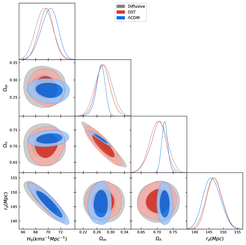
Figure 1: The posterior distribution with $1\sigma$ and $2\sigma$ for the DST, Diffusive and the $\Lambda$CDM model. The data set includes CC + Type Ia Supernova + Quasars + GRB + BAO. The Hubble function for the DST is from Eq. 24 and the Hubble function for the Diffusive model is from Eq. 52.

Table 1 summarizes the results for the RMV and the Diffusive model with a comparison to $\Lambda$CDM model. The posterior distribution is presented in figure 1, and the corresponding relation between the Hubble parameter and the additional parameter $\beta$ is presented in fig 2. The $\Omega_{\_}m$ matter part in the DST model $0.2780\pm 0.0214$ which is close for the Diffusive case. For the $\Lambda$CDM case the matter part is $0.263\pm 0.208$. The dark energy $\Omega_{\_}\Lambda$ part for the DST case $0.703\pm 0.024$, for the Diffusive case $0.704\pm 0.0203$ and for the $\Lambda$CDM case $0.728\pm 0.009$. The Hubble parameter for the DST case is lower then other cases: $69.63\pm 1.10$ for DST, $69.33\pm 1.24$ for Diffusive case of $70.40\pm 1.174\,(km/Sec/Mpc)$ for $\Lambda$CDM model.

The BAO scale is set by the redshift at the drag epoch $z_{\_}d\approx 1020$ when photons and baryons decouple [106]. For a flat $\Lambda$CDM, the Planck measurements yield $147.09\pm 0.26Mpc$ and the WMAP fit gives $152.99\pm 0.97Mpc$ [107]. Final measurements from the completed SDSS lineage of experiments in large-scale structure provide $r_{\_}d=149.3\pm 2.8Mpc$ [108].

The $\Lambda$CDM model for the combined data set we use gives $145.5\pm 2.66$. However, the DST model gives $147.1\pm 2.45$, while for the Diffusive case we obtain $146.7\pm 2.64$. The $r_{\_}d$ is in a moderate and reasonable range.

Figure 2: The posterior distribution for different measurements with $1\sigma$ and $2\sigma$ for the Hubble parameter.

From the AIC we see that $\Lambda$CDM is still the better fit to the late universe, since the AIC for $\Lambda$CDM model $264.7$ is lower then the DST case $267.0$ or for the Diffusive model case $269.9$.

6 Discussion

We know though $\Lambda$CDM could be the simplest phenomenological explanation for the observed acceleration of the Universe, there still exist a disagreement between the predicted and observed value of $\Lambda$. In particular, we are still facing the crucial question whether $\Lambda$ is truly a fundamental constant or a mildly evolving dynamical variable. It turns out that the $\Lambda=$const, despite being the simplest, may well not be the most favored one when compared with specific dynamical models of the vacuum energy. It also is unable to solve the tension related to the Hubble constant. Recently it has been shown the RVM are good modified models candidates to solve the Hubble tension. However, the model does not consider a Lagrangian formulation directly.

We obtain a candidate for the RVM formulated by an action principle that approaches the RVM of the second type asymptotically, without the requirement of dark components. We study this in dynamical space time vector model and also its diffusive extension. The scalar field model takes care of the behavior of the dark components. The kinetic term mimics the behavior of the dark matter and the potential terms acts like dark energy. Because of conformal invariance, the radiation cannot deviate from $1/a^{4}$ in this scenario. Analysing asymptotically, we have found that the DST and its diffusive counterpart have a different correspondence to the RVM.

We use CC + Type Ia Supernova + Quasars + GRB + BAO sets in order to constraint the model. It seems from the AIC test that the $\Lambda$CDM model is a better fit then DST and also the Diffusive case. However we can recover $\Lambda$CDM model by setting $\lambda_{\_}2=0$, and the $\Lambda$CDM in this case is formulated via an action principle.

References

- [1] Steven Weinberg. The Cosmological Constant Problem. Rev. Mod. Phys., 61:1–23, 1989. [,569(1988)].
- [2] Lucas Lombriser. On the cosmological constant problem. Phys. Lett., B797:134804, 2019.
- [3] Joshua Frieman, Michael Turner, and Dragan Huterer. Dark Energy and the Accelerating Universe. Ann. Rev. Astron. Astrophys., 46:385–432, 2008.
- [4] Fotios K. Anagnostopoulos and Spyros Basilakos. Constraining the dark energy models with data: An approach independent of . Phys. Rev., D97(6):063503, 2018.
- [5] Emmanuel N. Saridakis, Kazuharu Bamba, R. Myrzakulov, and Fotios K. Anagnostopoulos. Holographic dark energy through Tsallis entropy. JCAP, 1812:012, 2018.
- [6] Fotios K. Anagnostopoulos, Spyros Basilakos, Georgios Kofinas, and Vasilios Zarikas. Constraining the Asymptotically Safe Cosmology: cosmic acceleration without dark energy. JCAP, 1902:053, 2019.
- [7] Spyros Basilakos and Fotios K. Anagnostopoulos. Growth index of matter perturbations in the light of Dark Energy Survey. Eur. Phys. J., C80(3):212, 2020.
- [8] Fotios K. Anagnostopoulos, Spyros Basilakos, and Emmanuel N. Saridakis. Bayesian analysis of gravity using data. Phys. Rev., D100(8):083517, 2019.
- [9] Sunny Vagnozzi. New physics in light of the tension: an alternative view. 2019.
- [10] David Vasak, Johannes Kirsch, Dirk Kehm, and Juergen Struckmeier. Locally contorted space-time invokes inflation, dark energy, and a non-singular Big Bang. 2019.
- [11] Weiqiang Yang, Eleonora Di Valentino, Olga Mena, Supriya Pan, and Rafael C. Nunes. All-inclusive interacting dark sector cosmologies. Phys. Rev., D101(8):083509, 2020.
- [12] Eleonora Di Valentino. A (brave) combined analysis of the late time direct measurements and the impact on the Dark Energy sector. 2020.
- [13] Eleonora Di Valentino and Olga Mena. A fake Interacting Dark Energy detection? 2020.
- [14] H. B. Benaoum, Weiqiang Yang, Supriya Pan, and Eleonora Di Valentino. Modified Emergent Dark Energy and its Astronomical Constraints. 2020.
- [15] Weiqiang Yang, Eleonora Di Valentino, Supriya Pan, and Olga Mena. A complete model of Phenomenologically Emergent Dark Energy. 2020.
- [16] Eleonora Di Valentino, Eric V. Linder, and Alessandro Melchiorri. Ex Machina: Vacuum Metamorphosis and Beyond . 2020.
- [17] Eleonora Di Valentino, Stefano Gariazzo, Olga Mena, and Sunny Vagnozzi. Soundness of Dark Energy properties. 2020.
- [18] Weiqiang Yang, Eleonora Di Valentino, Olga Mena, and Supriya Pan. Dynamical Dark sectors and Neutrino masses and abundances. Phys. Rev., D102(2):023535, 2020.
- [19] Robert J. Scherrer. Purely kinetic k-essence as unified dark matter. Phys. Rev. Lett., 93:011301, 2004.
- [20] Alexandre Arbey. Dark fluid: A Complex scalar field to unify dark energy and dark matter. Phys. Rev., D74:043516, 2006.
- [21] Xi-ming Chen, Yun-gui Gong, and Emmanuel N. Saridakis. Phase-space analysis of interacting phantom cosmology. JCAP, 0904:001, 2009.
- [22] Genly Leon, Joel Saavedra, and Emmanuel N. Saridakis. Cosmological behavior in extended nonlinear massive gravity. Class. Quant. Grav., 30:135001, 2013.
- [23] Eduardo Guendelman, Emil Nissimov, and Svetlana Pacheva. Dark Energy and Dark Matter From Hidden Symmetry of Gravity Model with a Non-Riemannian Volume Form. Eur. Phys. J., C75(10):472, 2015.
- [24] Denitsa Staicova and Michail Stoilov. Cosmological solutions from models with unified dark energy and dark matter and with inflaton field. Springer Proc. Math. Stat., 255:251–260, 2017.
- [25] Genly Leon and Emmanuel N. Saridakis. Dynamical analysis of generalized Galileon cosmology. JCAP, 1303:025, 2013.
- [26] Georgios Kofinas, Genly Leon, and Emmanuel N. Saridakis. Dynamical behavior in cosmology. Class. Quant. Grav., 31:175011, 2014.
- [27] Maria A. Skugoreva, Emmanuel N. Saridakis, and Alexey V. Toporensky. Dynamical features of scalar-torsion theories. Phys. Rev., D91:044023, 2015.
- [28] Eduardo Guendelman, Emil Nissimov, and Svetlana Pacheva. Unified Dark Energy and Dust Dark Matter Dual to Quadratic Purely Kinetic K-Essence. Eur. Phys. J., C76(2):90, 2016.
- [29] Eduardo Guendelman, Emil Nissimov, and Svetlana Pacheva. Quintessential Inflation, Unified Dark Energy and Dark Matter, and Higgs Mechanism. Bulg. J. Phys., 44(1):015–030, 2017.
- [30] George Koutsoumbas, Konstantinos Ntrekis, Eleftherios Papantonopoulos, and Emmanuel N. Saridakis. Unification of Dark Matter - Dark Energy in Generalized Galileon Theories. JCAP, 1802:003, 2018.
- [31] Zbigniew Haba, Aleksander Stachowski, and Marek Szydlowski. Dynamics of the diffusive DM-DE interaction – Dynamical system approach. JCAP, 1607:024, 2016.
- [32] David Benisty and E. I. Guendelman. Interacting Diffusive Unified Dark Energy and Dark Matter from Scalar Fields. Eur. Phys. J., C77(6):396, 2017.
- [33] David Benisty and E. I. Guendelman. Unified DE–DM with diffusive interactions scenario from scalar fields. Int. J. Mod. Phys., D26(12):1743021, 2017.
- [34] Denitsa Staicova and Michail Stoilov. Cosmological aspects of a unified dark energy and dust dark matter model. Mod. Phys. Lett., A32(01):1750006, 2016.
- [35] Alejandro Perez, Daniel Sudarsky, and Edward Wilson-Ewing. Resolving the tension with diffusion. 2020.
- [36] Weiqiang Yang, Supriya Pan, Eleonora Di Valentino, Rafael C. Nunes, Sunny Vagnozzi, and David F. Mota. Tale of stable interacting dark energy, observational signatures, and the tension. JCAP, 1809:019, 2018.
- [37] Francesco D’Eramo, Ricardo Z. Ferreira, Alessio Notari, and José Luis Bernal. Hot Axions and the tension. JCAP, 1811:014, 2018.
- [38] Weiqiang Yang, Ankan Mukherjee, Eleonora Di Valentino, and Supriya Pan. Interacting dark energy with time varying equation of state and the tension. Phys. Rev., D98(12):123527, 2018.
- [39] Rui-Yun Guo, Jing-Fei Zhang, and Xin Zhang. Can the tension be resolved in extensions to CDM cosmology? JCAP, 1902:054, 2019.
- [40] Suresh Kumar, Rafael C. Nunes, and Santosh Kumar Yadav. Dark sector interaction: a remedy of the tensions between CMB and LSS data. Eur. Phys. J., C79(7):576, 2019.
- [41] Prateek Agrawal, Francis-Yan Cyr-Racine, David Pinner, and Lisa Randall. Rock ’n’ Roll Solutions to the Hubble Tension. 2019.
- [42] Weiqiang Yang, Supriya Pan, Eleonora Di Valentino, Andronikos Paliathanasis, and Jianbo Lu. Challenging bulk viscous unified scenarios with cosmological observations. Phys. Rev., D100(10):103518, 2019.
- [43] Weiqiang Yang, Olga Mena, Supriya Pan, and Eleonora Di Valentino. Dark sectors with dynamical coupling. Phys. Rev., D100(8):083509, 2019.
- [44] David Benisty, Eduardo I. Guendelman, and Emmanuel N. Saridakis. The Scale Factor Potential Approach to Inflation. 2019.
- [45] David Benisty, Eduardo I. Guendelman, Emmanuel N. Saridakis, Horst Stoecker, Jurgen Struckmeier, and David Vasak. Inflation from fermions with curvature-dependent mass. Phys. Rev., D100(4):043523, 2019.
- [46] David Benisty and Eduardo I. Guendelman. Inflation compactification from dynamical spacetime. Phys. Rev., D98(4):043522, 2018.
- [47] Eleonora Di Valentino, Alessandro Melchiorri, Olga Mena, and Sunny Vagnozzi. Nonminimal dark sector physics and cosmological tensions. Phys. Rev., D101(6):063502, 2020.
- [48] Eleonora Di Valentino, Alessandro Melchiorri, Olga Mena, and Sunny Vagnozzi. Interacting dark energy after the latest Planck, DES, and measurements: an excellent solution to the and cosmic shear tensions. 2019.
- [49] Joan Solà, Adria Gómez-Valent, and Javier de Cruz Pérez. First evidence of running cosmic vacuum: challenging the concordance model. Astrophys. J., 836(1):43, 2017.
- [50] Mehdi Rezaei, Mohammad Malekjani, and Joan Sola. Can dark energy be expressed as a power series of the Hubble parameter? Phys. Rev., D100(2):023539, 2019.
- [51] Adrià Gómez-Valent, Joan Solà, and Spyros Basilakos. Dynamical vacuum energy in the expanding Universe confronted with observations: a dedicated study. JCAP, 1501:004, 2015.
- [52] Joan Sola, Adria Gomez-Valent, and Javier de Cruz Pérez. Hints of dynamical vacuum energy in the expanding Universe. Astrophys. J. Lett., 811:L14, 2015.
- [53] Joan Solà Peracaula, Javier de Cruz Pérez, and Adria Gomez-Valent. Possible signals of vacuum dynamics in the Universe. Mon. Not. Roy. Astron. Soc., 478(4):4357–4373, 2018.
- [54] Joan Sola. Dark energy: A Quantum fossil from the inflationary Universe? J. Phys., A41:164066, 2008.
- [55] Pavlina Tsiapi and Spyros Basilakos. Testing dynamical vacuum models with CMB power spectrum from Planck. Mon. Not. Roy. Astron. Soc., 485(2):2505–2510, 2019.
- [56] Spyros Basilakos, Nick E. Mavromatos, and Joan Solà. Starobinsky-like inflation and running vacuum in the context of Supergravity. Universe, 2(3):14, 2016.
- [57] Christine R. Farrugia, Joseph Sultana, and Jurgen Mifsud. Endowing with a dynamic nature: Constraints in a spatially curved universe. Phys. Rev., D102(2):024013, 2020.
- [58] Nick E. Mavromatos. Supersymmetry, Cosmological Constant and Inflation: Towards a fundamental cosmic picture via ”running vacuum”. EPJ Web Conf., 126:02020, 2016.
- [59] Spyros Basilakos, Nick E. Mavromatos, and Joan Solà Peracaula. Gravitational and Chiral Anomalies in the Running Vacuum Universe and Matter-Antimatter Asymmetry. Phys. Rev., D101(4):045001, 2020.
- [60] Spyros Basilakos, Nick E. Mavromatos, and Joan Solà Peracaula. Do we Come from a Quantum Anomaly? Int. J. Mod. Phys., D28(14):1944002, 2019.
- [61] Spyros Basilakos, Nick E. Mavromatos, and Joan Solà Peracaula. Quantum Anomalies, Running Vacuum and Leptogenesis: an Interplay. PoS, CORFU2018:044, 2019.
- [62] Adria Gomez-Valent and Joan Sola. Relaxing the -tension through running vacuum in the Universe. EPL, 120(3):39001, 2017.
- [63] Evgeny A. Novikov. Ultralight gravitons with tiny electric dipole moment are seeping from the vacuum. Mod. Phys. Lett., A31(15):1650092, 2016.
- [64] Evgeny A. Novikov. Quantum Modification of General Relativity. Electron. J. Theor. Phys., 13(35):79–90, 2016.
- [65] Joan Sola, Adria Gomez-Valent, Javier de Cruz Perez, and Cristian Moreno-Pulido. Brans-Dicke cosmology with a - term: a possible solution to CDM tensions. 2020.
- [66] Joan Sola. Cosmological constant and vacuum energy: old and new ideas. J. Phys. Conf. Ser., 453:012015, 2013.
- [67] E. I. Guendelman. Gravitational Theory with a Dynamical Time. Int. J. Mod. Phys., A25:4081–4099, 2010.
- [68] David Benisty and Eduardo I. Guendelman. Unified dark energy and dark matter from dynamical spacetime. Phys. Rev., D98(2):023506, 2018.
- [69] David Benisty and E. I. Guendelman. Radiation Like Scalar Field and Gauge Fields in Cosmology for a theory with Dynamical Time. Mod. Phys. Lett., A31(33):1650188, 2016.
- [70] E. I. Guendelman. Scale invariance, new inflation and decaying lambda terms. Mod. Phys. Lett., A14:1043–1052, 1999.
- [71] E. I. Guendelman and A. B. Kaganovich. Dynamical measure and field theory models free of the cosmological constant problem. Phys. Rev., D60:065004, 1999.
- [72] Denis Comelli. A Way to Dynamically Overcome the Cosmological Constant Problem. Int. J. Mod. Phys., A23:4133–4143, 2008.
- [73] Fotios K. Anagnostopoulos, David Benisty, Spyros Basilakos, and Eduardo I. Guendelman. Dark energy and dark matter unification from dynamical space time: observational constraints and cosmological implications. JCAP, 1906(06):003, 2019.
- [74] David Benisty and Eduardo I. Guendelman. A transition between bouncing hyper-inflation to CDM from diffusive scalar fields. Int. J. Mod. Phys., A33(20):1850119, 2018.
- [75] Sebastian Bahamonde, David Benisty, and Eduardo I. Guendelman. Linear potentials in galaxy halos by Asymmetric Wormholes. Universe, 4(11):112, 2018.
- [76] David Benisty, Eduardo Guendelman, and Zbigniew Haba. Unification of dark energy and dark matter from diffusive cosmology. Phys. Rev., D99(12):123521, 2019.
- [77] Raul Jimenez and Abraham Loeb. Constraining cosmological parameters based on relative galaxy ages. Astrophys. J., 573:37–42, 2002.
- [78] Michele Moresco, Licia Verde, Lucia Pozzetti, Raul Jimenez, and Andrea Cimatti. New constraints on cosmological parameters and neutrino properties using the expansion rate of the Universe to z~1.75. JCAP, 07:053, 2012.
- [79] M. Moresco et al. Improved constraints on the expansion rate of the Universe up to z 1.1 from the spectroscopic evolution of cosmic chronometers. JCAP, 1208:006, 2012.
- [80] Michele Moresco. Raising the bar: new constraints on the Hubble parameter with cosmic chronometers at z 2. Mon. Not. Roy. Astron. Soc., 450(1):L16–L20, 2015.
- [81] Michele Moresco, Lucia Pozzetti, Andrea Cimatti, Raul Jimenez, Claudia Maraston, Licia Verde, Daniel Thomas, Annalisa Citro, Rita Tojeiro, and David Wilkinson. A 6% measurement of the Hubble parameter at : direct evidence of the epoch of cosmic re-acceleration. JCAP, 1605:014, 2016.
- [82] D.M. Scolnic et al. The Complete Light-curve Sample of Spectroscopically Confirmed SNe Ia from Pan-STARRS1 and Cosmological Constraints from the Combined Pantheon Sample. Astrophys. J., 859(2):101, 2018.
- [83] Fotios K. Anagnostopoulos, Spyros Basilakos, and Emmanuel N. Saridakis. Observational constraints on Barrow holographic dark energy. Eur. Phys. J., C80(9):826, 2020.
- [84] Carl Roberts, Keith Horne, Alistair O. Hodson, and Alasdair Dorkenoo Leggat. Tests of CDM and Conformal Gravity using GRB and Quasars as Standard Candles out to . 2017.
- [85] Marek Demianski, Ester Piedipalumbo, Disha Sawant, and Lorenzo Amati. Cosmology with gamma-ray bursts: I. The Hubble diagram through the calibrated - correlation. Astron. Astrophys., 598:A112, 2017.
- [86] David Benisty and Denitsa Staicova. Testing Low-Redshift Cosmic Acceleration with the Complete Baryon Acoustic Oscillations data collection. 2020.
- [87] Will J. Percival et al. Baryon Acoustic Oscillations in the Sloan Digital Sky Survey Data Release 7 Galaxy Sample. Mon. Not. Roy. Astron. Soc., 401:2148–2168, 2010.
- [88] Florian Beutler, Chris Blake, Matthew Colless, D. Heath Jones, Lister Staveley-Smith, Lachlan Campbell, Quentin Parker, Will Saunders, and Fred Watson. The 6dF Galaxy Survey: Baryon Acoustic Oscillations and the Local Hubble Constant. Mon. Not. Roy. Astron. Soc., 416:3017–3032, 2011.
- [89] Nicolas G. Busca et al. Baryon Acoustic Oscillations in the Ly- forest of BOSS quasars. Astron. Astrophys., 552:A96, 2013.
- [90] Lauren Anderson et al. The clustering of galaxies in the SDSS-III Baryon Oscillation Spectroscopic Survey: Baryon Acoustic Oscillations in the Data Release 9 Spectroscopic Galaxy Sample. Mon. Not. Roy. Astron. Soc., 427(4):3435–3467, 2013.
- [91] Hee-Jong Seo et al. Acoustic scale from the angular power spectra of SDSS-III DR8 photometric luminous galaxies. Astrophys. J., 761:13, 2012.
- [92] Ashley J. Ross, Lado Samushia, Cullan Howlett, Will J. Percival, Angela Burden, and Marc Manera. The clustering of the SDSS DR7 main Galaxy sample – I. A 4 per cent distance measure at . Mon. Not. Roy. Astron. Soc., 449(1):835–847, 2015.
- [93] Rita Tojeiro et al. The clustering of galaxies in the SDSS-III Baryon Oscillation Spectroscopic Survey: galaxy clustering measurements in the low redshift sample of Data Release 11. Mon. Not. Roy. Astron. Soc., 440(3):2222–2237, 2014.
- [94] Julian E. Bautista et al. The SDSS-IV extended Baryon Oscillation Spectroscopic Survey: Baryon Acoustic Oscillations at redshift of 0.72 with the DR14 Luminous Red Galaxy Sample. Astrophys. J., 863:110, 2018.
- [95] E. de Carvalho, A. Bernui, G. C. Carvalho, C. P. Novaes, and H. S. Xavier. Angular Baryon Acoustic Oscillation measure at from the SDSS quasar survey. JCAP, 1804:064, 2018.
- [96] Metin Ata et al. The clustering of the SDSS-IV extended Baryon Oscillation Spectroscopic Survey DR14 quasar sample: first measurement of baryon acoustic oscillations between redshift 0.8 and 2.2. Mon. Not. Roy. Astron. Soc., 473(4):4773–4794, 2018.
- [97] T. M. C. Abbott et al. Dark Energy Survey Year 1 Results: Measurement of the Baryon Acoustic Oscillation scale in the distribution of galaxies to redshift 1. Mon. Not. Roy. Astron. Soc., 483(4):4866–4883, 2019.
- [98] Z. Molavi and A. Khodam-Mohammadi. Observational tests of Gauss-Bonnet like dark energy model. Eur. Phys. J. Plus, 134(6):254, 2019.
- [99] Natalie B. Hogg, Matteo Martinelli, and Savvas Nesseris. Constraints on the distance duality relation with standard sirens. 2020.
- [100] M. Martinelli et al. Euclid: Forecast constraints on the cosmic distance duality relation with complementary external probes. 2020.
- [101] N. Benitez et al. Measuring Baryon Acoustic Oscillations along the line of sight with photometric redshifs: the PAU survey. Astrophys. J., 691:241–260, 2009.
- [102] W. J. Handley, M. P. Hobson, and A. N. Lasenby. PolyChord: nested sampling for cosmology. Mon. Not. Roy. Astron. Soc., 450(1):L61–L65, 2015.
- [103] Antony Lewis. GetDist: a Python package for analysing Monte Carlo samples. 2019.
- [104] Kenneth P. Burnham and David R. Anderson. Multimodel inference: Understanding aic and bic in model selection. Sociological Methods & Research, 33(2):261–304, 2004.
- [105] Andrew R Liddle. Information criteria for astrophysical model selection. Mon. Not. Roy. Astron. Soc., 377:L74–L78, 2007.
- [106] Éric Aubourg et al. Cosmological implications of baryon acoustic oscillation measurements. Phys. Rev. D, 92(12):123516, 2015.
- [107] N. Aghanim et al. Planck 2018 results. VI. Cosmological parameters. Astron. Astrophys., 641:A6, 2020.
- [108] Shadab Alam et al. The Completed SDSS-IV extended Baryon Oscillation Spectroscopic Survey: Cosmological Implications from two Decades of Spectroscopic Surveys at the Apache Point observatory. 7 2020.