Planet formation and migration near the silicate sublimation front in protoplanetary disks

Abstract

Context. The increasing number of newly detected exoplanets at short orbital periods raises questions about their formation and migration histories. Planet formation and migration depend heavily on the structure and dynamics of protoplanetary disks. A particular puzzle that requires explanation arises from one of the key results of the Kepler mission, namely the increase in the planetary occurrence rate with orbital period up to 10 days for F, G, K and M stars.

Aims. We investigate the conditions for planet formation and migration near the dust sublimation front in protostellar disks around young Sun-like stars. We are especially interested in determining the positions where the drift of pebbles would be stopped, and where the migration of Earth-like planets and super-Earths would be halted.

Methods. For this analysis we use iterative 2D radiation hydrostatic disk models which include irradiation by the star, and dust sublimation and deposition depending on the local temperature and vapor pressure.

Results. Our results show the temperature and density structure of a gas and dust disk around a young Sun-like star. We perform a parameter study by varying the magnetized turbulence onset temperature, the accretion stress, the dust mass fraction, and the mass accretion rate. Our models feature a gas-only inner disk, a silicate sublimation front and dust rim starting at around 0.08 au, an ionization transition zone with a corresponding density jump, and a pressure maximum which acts as a pebble trap at around 0.12 au. Migration torque maps show Earth- and super-Earth-mass planets halt in our model disks at orbital periods ranging from 10 to 22 days.

Conclusions. Such periods are in good agreement with both the inferred location of the innermost planets in multiplanetary systems, and the break in planet occurrence rates from the Kepler sample at 10 days. In particular, models with small grains depleted produce a trap located at a 10-day orbital period, while models with a higher abundance of small grains present a trap at around a 17-day orbital period. The snow line lies at 1.6 au, near where the occurrence rate of the giant planets peaks. We conclude that the dust sublimation zone is crucial for forming close-in planets, especially when considering tightly packed super-Earth systems.

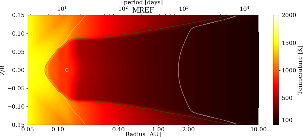
Figure 1: Temperature profile in the 2D R/Z plane for our reference model MREF, a young solar-type star with a radially-uniform mass accretion rate of $\rm 3.6\times 10^{-9}M_{\sun}/yr$, a dust-to-gas mass ratio for small grains of $0.001$ and stress-to-pressure ratios of $\alpha_{MRI}=0.01$ and $\alpha_{DZ}=0.001$. The green solid line shows optical depth $\tau=2/3$ for the starlight irradiation. The yellow dashed line shows the silicate sublimation front. The white solid line shows the water sublimation front. The white circle shows the location of the pebble trap, where large grains would concentrate.

1 Introduction

Our knowledge of the origins of planetary systems relies on our understanding of the disks of gas and dust orbiting young stars. With the growing number of detected exoplanetary systems, we want to learn about their formation and evolution, starting from their building blocks in young protoplanetary disks. One key result of the Kepler mission was the discovery of many planetary systems containing Earth-sized and super-Earth planets orbiting with periods between one day and one year (Lissauer et al., 2011; Batalha et al., 2013; Fabrycky et al., 2014). The Kepler mission focused on searching for planetary systems around F-, G-, and K-type stars. Further analysis of the results showed a clear rise in the occurrence rate of super-Earths (rocky planets of several Earth masses) with orbital periods longer than 10 days. The occurrence is uniform at longer periods (Youdin, 2011; Mulders et al., 2015; Petigura et al., 2018). Over recent years, possible mechanisms for this rise were investigated, including truncation of the disk by the stellar magnetosphere (Lee & Chiang, 2017), trapping of planets at the inner edge of the disk (Brasser et al., 2018; Carrera et al., 2019), and the removal of close-in planets by tidal interactions inside 10-day orbital periods (Rice et al., 2012). Even more recently, Mulders et al. (2018) have found, when including observational constraints on multiplanetary systems, that on average the innermost planet orbits with a 12-day period.

Broadly speaking, models of the formation of short-period planets are based either on the drift of pebbles to locations near the inner edge of the disk where they concentrate and grow into planets (Boley et al., 2014; Chatterjee & Tan, 2014) or on planets that form farther out in the disk, perhaps by pebble accretion (Lambrechts et al., 2019; Izidoro et al., 2019), and then migrate inward before reaching locations near the inner edge of the disk where migration halts because the disk-planet torques go to zero (Terquem & Papaloizou, 2007; Ida & Lin, 2010; Faure & Nelson, 2016; Izidoro et al., 2017). To compare these planet formation models with observations, the main disk property used is the abundance of solids (Dawson et al., 2015, 2016). Formation models are typically based on simple assumptions about the inner disk structure. More detailed self-consistent disk profiles of density and temperature including irradiation and dust sublimation have not yet been computed.

In this work our aim is to develop irradiated hydrostatic disk models around young Sun-like stars. With respect to the Kepler mission results, we want to address the influence of the disk structure on both pebble drift and planet migration, and in particular show how the temperature and density structure leads to locations where drifting pebbles and migrating planets are trapped.

We follow the numerical methods that we used previously to model the inner disk around Herbig Ae/Be-type stars (Flock et al., 2016). In this work, we have adapted all the parameters to match a protoplanetary disk around an early Sun-like star, which is less massive and less luminous than Herbig Ae/Be stars, and for which the disks sustain a higher mass accretion rate.

We first investigate the density and thermal structure of the disk, and its impact on pebble drift and planet migration. We consider steady-state models with a radially uniform mass accretion rate. To determine the surface density we use the temperature dependent $\alpha$ value, which we directly calculate from our previous 3D radiation magneto-hydrodynamic (MHD) simulations (Flock et al., 2017). In our previous work we found that the effect of viscous heating is small (Flock et al., 2016), and therefore we focus on passively heated disks in this work.

For temperatures below 850-1000K (which is dependent on the density), the ionization level drops (Desch & Turner, 2015) and turbulent activity due to the magneto-rotational instability (MRI) quickly decreases, mainly due to Ohmic resistivity (Thi et al., 2018). Among the main processes governing the temperatures in the region close to the star are the irradiation heating and sublimation of silicate grains, which change the opacity by orders of magnitude (Pollack et al., 1994), and which we include in these models.

The structure of the paper is as follows. In Section 2 we briefly review the main parts of the numerical method. In Section 3 we present the 2D radiation hydrostatic solutions. In Section 4 we calculate migration maps. Sections 5 and 6 follow with the discussion and conclusions.

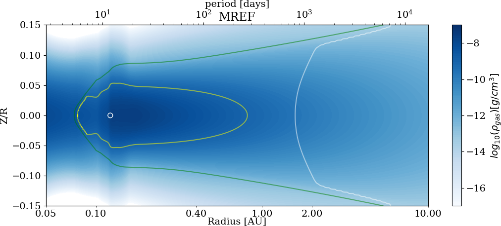
Figure 2: Density profile in the 2D plane of model MREF, a young solar-type star with a radially uniform mass accretion rate of $\rm 3.6\times 10^{-9}M_{\sun}/yr$, a dust-to-gas mass ratio for small grains of $0.001$ and stress-to-pressure ratios of $\alpha_{MRI}=0.1$ and $\alpha_{DZ}=0.001$. Contours of the gas and dust density are shown for $10^{-9}$ and $10^{-12}\rm g/cm^{3}$ (yellow solid line). The green solid line shows the optical depth line $\tau=2/3$ for the starlight irradiation. The white solid line shows the water snow line in the disk. The white circle shows the location of the pebble trap.

2 Method

We followed the previous numerical method presented by Flock et al. (2016). We first calculated a radiation hydrostatic equilibrium, solving iteratively the radiation transfer including irradiation. In the first step the gas surface density profile was determined using

$$\rm\Sigma(R)=\frac{\dot{M}}{3\pi\nu_{t}(R)}$$ (1)

at the cylindrical radius $\rm R$, assuming a constant radial mass accretion rate $\rm\dot{M}$. The viscosity is given by

$$\rm\nu_{t}=\frac{\alpha c_{s}^{2}}{\Omega}\,,$$ (2)

where $\rm c_{s}$ is the sound speed, $\rm\Omega=\sqrt{GM_{*}/R^{3}}$ is the disk rotation frequency, and the stress-to-pressure ratio is given by

$$\rm\alpha=(\alpha_{MRI}-\alpha_{DZ})\left[\frac{1-\tanh{\left(\frac{T_{MRI}-T}{25K}\right)}}{2}\right]+\alpha_{DZ}\,,$$ (3)

with $\alpha_{MRI}=0.01$ being the stress-to-pressure ratio in the active zone $(T>T_{MRI})$, $\alpha_{DZ}$ being the stress-to-pressure ratio in the dead zone, and $T_{MRI}$ being the ionization transition temperature for the MRI to operate.

The initial temperature field $\rm T(r,\theta)$ was calculated using the optically thin solution, which depends on the stellar luminosity and the opacities. We then calculated the density $\rm\rho(r,\theta)$ and azimuthal velocity $\rm v_{\phi}(r,\theta)$ by solving the governing equations in spherical coordinates $\rm(r,\theta,\phi)$ with axisymmetry to obtain the solution for hydrostatic equilibrium,

$$\rm\frac{\partial\mathrm{P}}{\partial\mathrm{r}} = -\rho\frac{\partial\Phi}{\partial\rm r}+\frac{\rho\rm v^{2}_{\phi}}{\rm r}$$ (4)

$$\rm\frac{1}{r}\frac{\partial\mathrm{P}}{\partial\theta} = \rm\frac{1}{\tan{\theta}}\frac{\rho v^{2}_{\phi}}{r}\,,$$ (5)

where $\rm\Phi$ is the gravitational potential $\rm\Phi=GM_{*}/r$ (with $\rm G$ being the gravitational constant and $\rm M_{*}$ the stellar mass) and $\rm P$ is the thermal pressure that relates to the temperature through the ideal-gas equation of state:

$$\rm P=\frac{\rho k_{B}T}{\mu_{g}u}$$ (6)

with the mean molecular weight $\rm\mu_{g}$, the Boltzmann constant $\rm k_{B}$, and the atomic mass unit $\rm u$.

For a given density field, the internal energy and radiation field in radiative equilibrium were obtained as the steady-state solution to the following coupled pair of equations describing heating, cooling, and the flux-limited diffusion of the disk’s thermal radiation:

$$\begin{split}\rm\frac{1}{\gamma-1}\partial_{t}P&=\rm-\kappa_{P}\rho\mathrm{c}(a_{R}T^{4}-E_{R})-\nabla\cdot F_{*},\\ \rm\partial_{t}E_{R}-\nabla\frac{c\lambda}{\kappa_{R}\rho}\nabla E_{R}&=\rm+\kappa_{P}\rho\mathrm{c}(\rm a_{R}T^{4}-E_{R}).\end{split}$$ (7)

Here we used the adiabatic index $\rm\gamma$, the radiation energy E_R, the irradiation flux $\mathrm{F}_{*}$, the flux limiter $\rm\lambda$ (Levermore & Pomraning, 1981), the Rosseland and Planck mean opacity $\rm\kappa_{R}$ and $\rm\kappa_{P}$, the radiation constant $\rm a_{R}=4\sigma_{b}/c$ (with the Stefan-Boltzmann constant $\rm\sigma_{b}$ and the speed of light c). We computed $\mathrm{F}_{*}$ by solving the transfer equation along radial rays from the central star, treated as a point source. Following our previous work, we simplified the problem by assuming $\rm\kappa_{R}=\kappa_{P}$ and considering three opacities: the gas opacity $\rm\kappa_{gas}$, the Planck dust opacity at the dust sublimation temperature $\rm\kappa_{P}(T_{s})$, and the Planck dust opacity at the stellar temperature $\rm\kappa_{P}(T_{*})$.

We took the gas opacities from Malygin et al. (2014) for starlight and for the disk’s thermal emission. The two dust opacities were frequency-averaged, one over the blackbody spectrum at the sublimation temperature and the other over the irradiating starlight spectrum. The combined opacity was determined using the dust-to-gas ratio. For details on the gas and dust opacities we refer to the Appendix.

We ignored the heat released by accretion within the disk. Viscosity was only used to set the constant mass accretion and to obtain a surface density profile consistent with the uniform mass accretion rate. In our previous work we found the effect of viscous heating remains small (Flock et al., 2016), while recent disk wind models predict an even smaller viscous heating effect (Béthune et al., 2017; Mori et al., 2019) in the dead-zone region. We address this again in the discussion section.

Convergence was reached by iteratively solving for the radiation equilibrium and hydrostatic equilibrium, including irradiation from the star. We iterated until we reached convergence. We iterated 30 times (compared to 20 times in our previous method) as these models span a larger domain.

2.1 Dust sublimation

As in our previous work, we followed Pollack et al. (1994) and used the fitting model of Isella & Natta (2005) that applies to situations for which the most refractory grains are silicates when determining the sublimation temperature:

$$\rm T_{s}=2000K\left(\frac{\rho}{1g\,cm^{-3}}\right)^{0.0195}\,.$$ (8)

The value of $\rm T_{s}$ was then used to calculate the dust-to-gas ratio $\rm f_{D2G}$, which is the ratio between the dust density $\rm\rho_{d}$ and the gas density. We slightly modified our previous formula (Eq. 11 in Flock et al. 2016) to

$$\rm f_{D2G}=\left\{\begin{array}[]{l}\rm f_{\Delta\tau}\left\{\frac{1-\tanh(\left(\frac{T-T_{s}}{100K}\right)^{3})}{2}\right\}\left\{\frac{1-\tanh(2/3-\tau_{*})}{2}\right\}\\ \rm f_{0}\,\rm for\,T<T_{s}\rm\,and\,\tau>3.0\end{array}\right.,$$ (9)

with the additional constraint that $\rm f_{D2G}\leq f_{0}$, with $\rm f_{0}$ being the maximum dust-to-gas mass ratio and $\rm f_{\Delta\tau}=0.2/(\rho_{dust}\Delta r\kappa_{P}(T_{*})$ being the dust amount to account for optical depth of $\Delta\tau=0.2$ for a given grid cell with radial width of $\rm\Delta r$. This value ensures that we resolve the absorption of the incoming radiation at the inner rim. We slightly steepened the transition compared to our previous work where we used $\Delta\tau=0.3$. We also centered the absorption at $\tau=2/3$ where most of the absorption happens at $\tau=2/3$.

For $\rm T<T_{s}$ and $\tau>3.0$ most of the irradiation is absorbed and the available silicates occur in solid form. For more information on the method, the flux limiter, and the treatment of the optical depth at the rim wall we refer to Flock et al. (2016).

3 Model parameters

The model input parameters are summarized in table 1 and table 2.

Stellar parameters	$\rm T_{*}=4300\,K$, $\rm R_{*}=2.6\,R_{\sun}$
	$\rm M_{*}=1.0\,M_{\sun}$
Opacity	$\rm\kappa_{P}(T_{*})=1300\,cm^{2}/g$
	$\rm\kappa_{P}(T_{s})=700\,cm^{2}/g$
	$\rm\kappa_{gas}\sim 10^{-5}\,cm^{2}/g$
Grid size $\rm N_{r}\times N_{\theta}$	2048 x 128
Cell aspect ratio	$\Delta R/R\Delta\theta\sim 1.1$
Radial domain $\rm R_{in}-R_{out}$	0.05-10 AU
Vertical domain $\rm Z/R$	$\pi/2\pm 0.15$
Ionization transition	$\rm T_{MRI}=900K$
$\alpha$ viscosity	$\alpha_{MRI}=10^{-2}$ for $T>T_{MRI}$
	$\alpha_{DZ}=10^{-3}$ for $T\leq T_{MRI}$
Dust-to-gas mass ratio	$\rm f_{0}=10^{-3}$
of small grains ($\leq 10\rm\mu m$)
Mass accretion rate	$\rm\dot{M}=3.6\times 10^{-9}M_{\sun}/yr$

Table 1: Parameters for the MREF model.

The stellar parameters were taken from a stellar evolution track by Siess et al. (2002) and D’Antona & Mazzitelli (1994), and represent a young solar star with an age of approximately one million years. Here we recalculated the stellar spectrum-weighted irradiation opacity. The redder spectrum of the T Tauri star reduces the irradiation opacity compared to our previous models, which were calculated for a Herbig-type star. The irradiation opacity $\rm\kappa_{P}(T_{*})$ is 1300 $\rm cm^{2}/g$ and the thermal emission opacity is $\rm\kappa_{P}(T_{s})=700\,cm^{2}/g$.

The dust-to-gas mass ratio ranges from $\rm 10^{-4}$ to $10^{-3}$ representing grains with sizes up to 10 $\rm\mu m$, which dominate the opacity at the relevant temperatures and wavelengths. Modeling indicates that most of the solid material is locked in larger grains (Birnstiel et al., 2012), consistent with a protostellar disk millimeter flux-radius correlation (Rosotti et al., 2019) and the weakness of silicate features in the infrared spectra of the disks around young stars with masses near solar (Furlan et al., 2006, 2009, 2011).

We investigated ionization transition temperatures of 900K and 1000K. For our reference model we assume 900K, motivated by the ionization thresholds, which are at cooler temperatures for higher densities (Desch & Turner, 2015). We studied accretion rates between $10^{-9}$ and $\rm 10^{-8}M_{\sun}/yr$ corresponding to those of disks in the Chamaeleon I star-forming region (Manara et al., 2017). For our reference model, MREF, we used a value of $\rm 3.6\times 10^{-9}M_{\sun}/yr$. We note that as we did not include the outer edge of the disk in our models, the total disk mass remains a free parameter.

For the stress-to-pressure ratio $\alpha_{MRI}$ in the MRI active region, we took values between $0.01$ and $0.1$. The larger value was determined from our previous 3D radiation non-ideal MHD simulations. In Flock et al. (2017) we found a stress-to-pressure ratio of up to 0.1 for the net vertical magnetic flux case. For temperatures below the ionization threshold we chose stress-to-pressure ratios $\alpha_{DZ}$ between $10^{-3}$ and $5\times 10^{-4},$ to mimic the accretion activity either by hydrodynamical instabilities (Lyra & Umurhan, 2019) or a magnetically driven wind (Béthune et al., 2017). We note again that the increase in the stress-to-pressure ratio at the ionization transition has a direct impact on the surface density profile. Compared to our previous models (Flock et al., 2016) we also investigated larger jumps in $\alpha$ and the surface density.

The grid resolution is 2048 cells in radius logarithmically spaced and 128 in the meridional direction for a domain extending from 0.05 to 10 AU in radius and to elevation angles 0.15 radians on either side of the equatorial plane in the meridional direction. The inner radial boundary was chosen to be close to but still outside the radius where the stellar magnetic field is expected to truncate the disk.

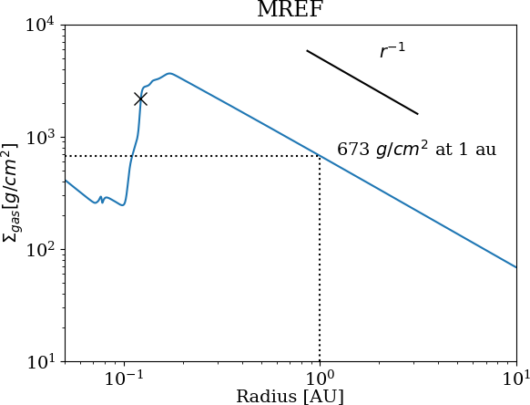
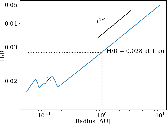
Figure 3: Top: Radial profile of the gas surface density for our reference model MREF. The steep rise at around 0.11 au is due to the drop in the accretion stress. Bottom: Profile of the midplane scale height H/R. The markings in the panels show the values at 1 au (dotted lines), the position of the pebble trap (black cross, $\times$) and typical slope profiles for comparison (black lines).

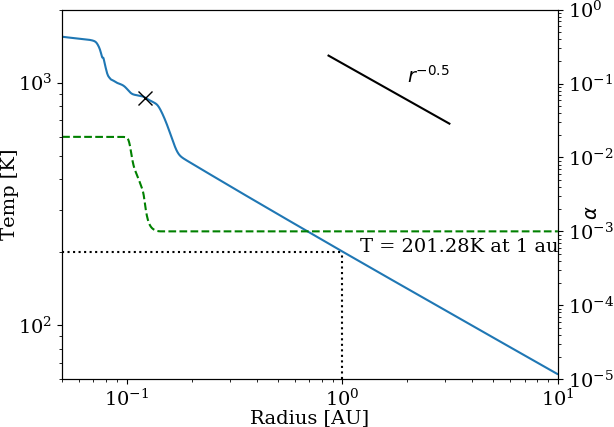
Figure 4: Radial profile of the disk midplane temperature. Shown in the plot are the values at 1 au and the position of the pebble trap (black cross, $\times$). The midplane stress-to-pressure ratio $\alpha$ is overplotted (green dashed line).

4 Results

The results derived from the radiation hydrostatic solution for our reference model are shown in Fig. 1 and Fig. 2. Figure 1 presents the 2D temperature profile of the disk, showing a similar structure to that found for a Herbig-type star (Flock et al., 2016), but where the key features occur on smaller radial scales closer to the star: a hot dust halo in front of the rim inside 0.08 au, a curved dust rim between 0.08 and 0.15 au, a small shadowed region between 0.2 and 0.3 au, and a flared disk beyond 0.3 au. The starlight optical depth $\tau=2/3$ line starts at the midplane at 0.08 au, while reaching an elevation angle of $\rm\theta=0.08rad$ at 0.15 au. At 8 au the $\tau=2/3$ line reaches $\theta=0.15$, which corresponds to roughly 3 scale heights. We find a pressure maximum and pebble trap located at 0.12 au, indicated by a white circle in Fig. 1. In this region, inward drifting pebbles are trapped, and could possibly trigger planetesimal formation. Figure 2 presents the corresponding 2D gas density profile. The next feature with increasing distance from the star is the rise in gas density at 0.13 au due to the lower stress-to-pressure ratio at temperatures below the ionization threshold. Midplane densities of $\rm 10^{-8}\,gcm^{-3}$ are reached in the gas. The density jump is clear in the gas surface density profile in the top panel of Fig. 3. For this model we obtain a gas surface density of 680 $\rm g/cm^{2}$ at 1 au. Figures 3 and  4 show the radial profile of the disk scale-height–to–radius ratio ($H/R$) and the midplane temperature. Near the silicate sublimation front the $H/R$ is around 0.02, generally increasing outward to reach $0.028$ at 1 au. The disk radial temperature shows the typical profile, with a shallower decrease at the rim at around 1000 K, while at 1 au the temperature reaches roughly 200 K. For comparison, Fig. 3 and Fig. 4 also show the slopes for $r^{-1}$ for density, $r^{2/7}$ for $H/R$, and $r^{-0.5}$ for the temperature.

Figures 1 and  2 both include the snow line. We locate the snow line using the water vapor mole fraction

$$X_{H_{2}O}=\left\{\begin{array}[]{ll}1.2\times 10^{-3}\,\,(1.2\times 10^{-3}P\leq P_{sat}(T)),\\ P_{sat}(T)/P\,\,(1.2\times 10^{-3}P\geq P_{sat}(T)),\\ \end{array}\right.$$ (10)

(Oka et al., 2011) with a total water mole fraction of $1.2\times 10^{-3}$ and a saturated vapor pressure

$$P_{sat}=e^{-6070K/T+30.86}dyn\,cm^{-2}.$$ (11)

In Fig. 1 we determine the position where half of the water is in the form of ice, such that $x_{ice}=0.5$, using

$$x_{ice}=1-X_{H_{2}O}/(1.2\times 10^{-3}).$$ (12)

Using this formula we determine that the snow line crosses the midplane at 1.6 au, reaching 2 au at 2 scale heights above the midplane. Due to the lower pressure and higher temperature, the snow line moves radially outward with increasing vertical height until it reaches 7 au at 3 scale heights. The snow line is an important location for planet formation. In particular, due to the predicted agglomeration of larger grains this is a preferred location of giant planet formation (Oka et al., 2011; Ros & Johansen, 2013; Drażkowska & Alibert, 2017; Schoonenberg et al., 2018). We note that for our choice of stellar parameters and resulting stellar luminosity of $\sim 1.92L_{\sun}$ the snow line is located farther out radially compared to models with a lower stellar luminosity. This value is similar to recent solar-mass and metallicity stellar models (Amard et al., 2019), which predict roughly 2 $L_{\sun}$ for a star one million years in age.

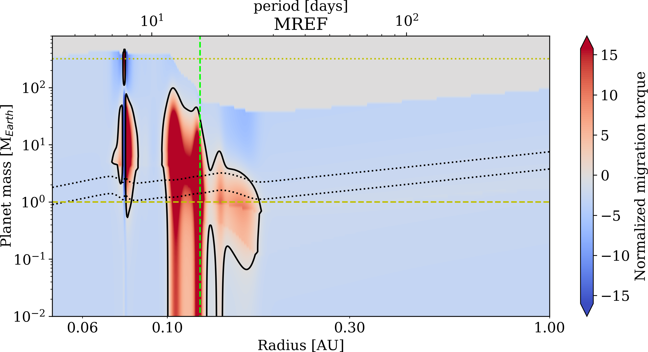
Figure 5: Normalized total orbital migration torque ($\Gamma_{\rm tot}/\Gamma_{0}$) vs. planetary mass and orbital radius in the reference model MREF, zoomed into the region inside 1 au. Inward migration is shown in blue, while outward migration is shown in red. The solid black line marks where the migration torque is zero, and hence where planets are trapped. Dotted lines indicate the pebble isolation mass, following Lambrechts et al. (2014) (lower) and Bitsch et al. (2018) (upper). The green dashed line indicates the location of the pebble trap, where the inward radial drift of solid particles halts. The gray shading at the top shows the gap-opening region according to Crida et al. (2006). Here, planets would modify the surface density structure strongly. The horizontal yellow dashed and dotted lines indicate the masses of Earth and Jupiter.

Model	$T_{MRI}$	$\alpha_{MRI}$	$\alpha_{DZ}$	$\dot{M}$	$f_{0}$	$\kappa_{gas}$	trap
MREF	900	0.01	$10^{-3}$	$3.6\cdot 10^{-9}$	$10^{-3}$	$10^{-5}$	0.12
M0	900	0.05	$10^{-3}$	$3.6\cdot 10^{-9}$	$10^{-3}$	$10^{-5}$	0.13
M1	900	0.05	$10^{-3}$	$3.6\cdot 10^{-9}$	$10^{-4}$	$10^{-5}$	0.093
M2	900	0.1	$10^{-3}$	$3.6\cdot 10^{-9}$	$10^{-3}$	$10^{-5}$	0.13
M3	900	0.05	$5\cdot 10^{-4}$	$3.6\cdot 10^{-9}$	$10^{-3}$	$10^{-5}$	0.15
M4	900	0.05	$10^{-3}$	$10^{-8}$	$10^{-3}$	$10^{-5}$	0.15
M5	900	0.05	$10^{-3}$	$10^{-9}$	$10^{-3}$	$10^{-5}$	0.13
M6	$10^{3}$	0.05	$10^{-3}$	$3.6\cdot 10^{-9}$	$10^{-3}$	$10^{-5}$	0.12
M7	900	0.05	$10^{-3}$	$3.6\cdot 10^{-9}$	$10^{-3}$	$10^{-4}$	0.13

Table 2: Model name, ionization transition in Kelvin, MRI $\alpha$ value, $\alpha$ in the dead zone, mass accretion rate in $[M_{\sun}/yr]$, dust-to-gas mass ratio, gas opacity in $\rm[cm^{2}/g]$, and resulting location of the pebble trap in au.

4.1 Migration maps

In this section we calculate the migration torques on planets embedded in our reference model. We are especially interested in determining where orbital migration halts, as this may set up the architecture of the new planetary system.

We use the torque formula from Paardekooper et al. (2011) as adapted by Bitsch & Kley (2011). The total torque $\Gamma_{tot}$ is the sum of the Lindblad torque $\Gamma_{L}$ and the corotation torque $\Gamma_{c}$. The Lindblad torque arises because of the spiral waves launched at the planet’s Lindblad resonances. We follow Paardekooper & Papaloizou (2008) and write

$$\Gamma_{L}=\frac{\Gamma_{0}}{\gamma}\left(-2.5-1.7\beta^{s}+0.1\alpha^{s}\right)$$ (13)

with $\alpha^{s}$ the negative slope of the surface density profile $\Sigma\propto r^{-\alpha^{s}}$ and $\beta^{s}$ the negative slope of the temperature profile $T\propto r^{-\beta^{s}}$. The normalization torque $\Gamma_{0}$ is defined as

$$\Gamma_{0}=\left(\frac{q}{h}\right)^{2}\Sigma_{P}r_{P}^{4}\Omega_{P}^{2}$$ (14)

with $q$ the planet-to-star mass ratio, $h$ the aspect ratio $h=H/R$, $\Sigma_{P}$ the surface density at the planet’s location $r_{P}$, and $\Omega_{P}$ the orbital frequency of the planet. Calculating the corotation torque $\Gamma_{c}$ is more complicated because this can saturate at a level depending on planet mass, disk viscosity, and local thermal diffusion rate. We compute $\Gamma_{c}$ as detailed in Sects. 5.6 and 5.7 of Paardekooper et al. (2011).

The above calculation of $\Gamma_{tot}$ is valid until the gap-opening or type II migration regime is reached. To determine the gap-opening mass we follow the equation by Crida et al. (2006):

$$\frac{3}{4}\frac{H}{R_{H}}+\frac{50}{qRe}=1.0,$$ (15)

with the Hill radius

$$R_{H}=R_{p}\left(\frac{q}{3}\right)^{1/3}$$ (16)

and the Reynolds number

$$Re=R_{p}^{2}\Omega_{p}/\nu_{t}.$$ (17)

Planets exceeding this mass would substantially change the surface density structure, and hence the migration torque.

In Fig. 5 we present a map of the total torque in the planet orbital radius-mass plane. For this calculation, the values of the density, temperature, stress-to-pressure ratio, surface density, and opacity are all taken from the reference radiation hydrostatic solution which is in inflow equilibrium. The figure shows that across most of the inner disk and for most planetary masses, migration is inward, as expected from type I migration models (Ward, 1997; Fogg & Nelson, 2007; Crida & Bitsch, 2017). From left to right, the first region of outward migration is connected to the dust sublimation zone at around 0.08 au and the resulting drop in temperature. This region is relevant only for planets more massive than the Earth and it could be a halting point for planets all the way up to the gap-opening mass.

The next and most prominent region of outward migration lies in the steep rise of the surface density starting at 0.1 au. Here outward migration occurs for planets with masses from as low as 1% of an Earth mass and up to 100 Earth masses. The normalized migration torque is very strong, reaching $\Gamma_{\rm tot}/\Gamma_{0}\geq 15$. Such a planet trap at surface density transition was already proposed by Masset et al. (2006). The third outward migration region is due to the small shadowed zone where the temperature drops significantly starting at 0.13 au. This outward migration region affects planets with masses between 0.1 and 4 Earths. The radii where the torque vanishes (black solid contour lines) are especially interesting for planet formation and evolution models. At these locations, the Lindblad and corotation torques exactly cancel each other.

In Fig. 5 we overplot with a vertical green dashed line the location of the pressure maximum where inward-drifting pebbles accumulate. This location approximately coincides with the planet migration trap. If a steady radial drift of pebbles is present, we might expect a first planetary core to form at this location. Growth by accreting pebbles could continue until the planet reaches the pebble isolation mass. Lambrechts et al. (2014) found the pebble isolation mass to be

$$M_{iso}=20M_{Earth}\left(\frac{h}{0.05}\right)^{3}.$$ (18)

Recently, Bitsch et al. (2018) found that the pebble isolation mass can, for certain parameters, be a factor of two higher than the fit by Lambrechts et al. (2014). In Fig. 5 we show both estimates. From this calculation we expect the planets to form at the pebble trap near 0.13 au and to have masses between 1.5 and 3 Earth masses.

Finally, gray shading indicates the region of type II migration where the planet’s tides would be strong enough to open a gap. Such a drastic change in the disk structure means the migration torque calculation is invalid in this region. We also note that we do not see any change in the migration zones radially outward between 1 and 10 au. In Sect. 4.3 we compare these results with the exoplanet occurrence rate obtained from the Kepler sample.

4.2 Parameter study

In this section we vary the parameters (see Table 2). A summary of the resulting temperature and surface density profiles is in Fig. 6. Increasing the value of $\alpha_{MRI}$ in the inner disk in model M0 compared to MREF leads to a steeper gradient in the surface density. This also affects the planet trap, extending the zero-torque region to larger planet masses (see Appendix A). The position of the pebble trap is shifted outward by only 0.01 au. Decreasing the abundance of small grains, and hence the opacity, has a larger effect. Decreasing the dust-to-gas ratio to $10^{-4}$ in model M1 shifts the inner rim closer to the star, and results in a steeper rise in the temperature at the rim. The pebble trap moves radially inward to 0.093 au, corresponding to a 10-day orbital period. The other noticeably different model is M4 with the highest abundance of small grains, which shifts the pebble trap to 0.15 au, corresponding to a 22-day orbital period. Increasing the gas opacity by one order of magnitude in model M7 had only a small effect on the structure as the gas between the sublimation front and the star remains optically thin.

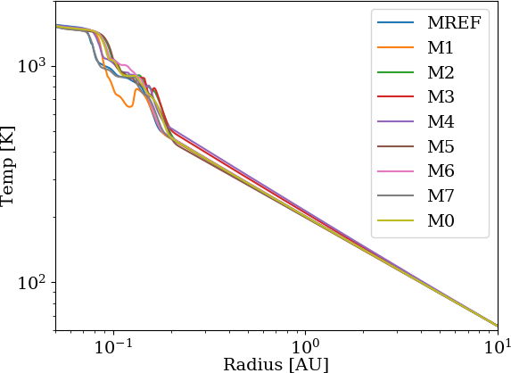
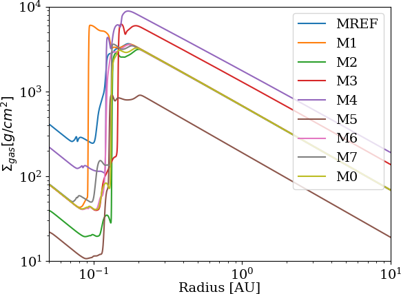
Figure 6: Temperature and surface density profiles over radius for all models.

4.3 Comparison with exoplanet occurrence rates

In this section we compare our results with previous analyses of exoplanet occurrence rates. We note that for all models we use a fixed stellar type, while the Kepler sample is based on a mix of F-, G-, and K-type stars.

In the top panel of Fig. 7 we show the inferred real distribution of the orbital period of the innermost planet in Kepler multiplanetary systems reported by Mulders et al. (2018). Overplotted are the positions of the pebble traps we found in our models.

The pebble trap in our models reproduces quite well the position of the innermost planet in multiplanetary systems. The pebble trap occurs slightly farther from the star, with a mean orbital period of around 17 days. The dust-depleted model, M1, matches the 10-day peak in the measured planets’ distribution. Mulders et al. (2018) show that the innermost planets had between one and four Earth radii, roughly corresponding to between one and ten Earth masses. Interestingly, this is similar to the mass range of the type I migration trap (Fig. 5). The scatter in the measured radii (and masses, assuming a an Earth-like density) of the innermost planets is consistent with the range from the pebble isolation mass up to the gap-opening threshold.

The innermost planet trap in Fig. 5 is located near an 8-day orbital period and connected with the dust sublimation front. Inward-migrating super-Earths can also pile up at the planet trap at the inner edge of the gas disk where a cavity forms because of the stellar magnetosphere. That inner-edge trap sits closer to the star than the trap in our models, which is a result of the transition between the inner MRI-active region and the dead zone. We further note that multiplanetary systems in resonant chains can push the innermost planets farther in (Carrera et al., 2018; Izidoro et al., 2019; Carrera et al., 2019).

In the bottom panel of Fig. 7 we show the results of Fernandes et al. (2018) for the occurrence rate of giant planets from RV surveys and Kepler. They find a clear peak around 2 au, which is very close to the predicted position of the snow line in our models.

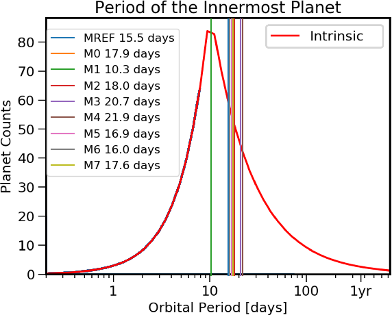
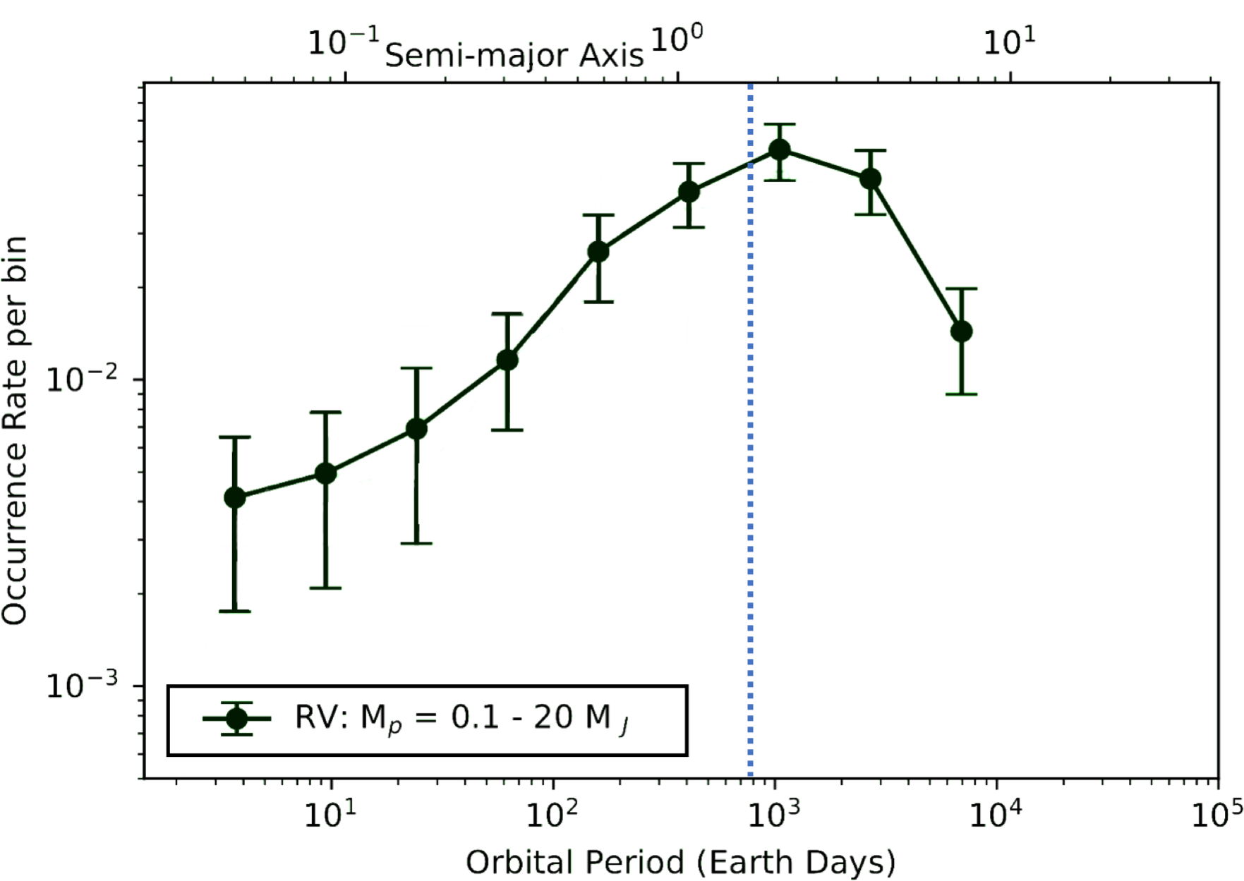
Figure 7: Top: Orbital period of the innermost planet in Kepler multiplanetary systems, taken from Mulders et al. (2018). Overplotted are the positions of the pressure maxima for our models. Bottom: Giant planet occurrence rate for RV and Kepler surveys (Fernandes et al., 2018). The blue dashed line indicates the position of the snow line in our models.

4.4 Dependence on luminosity

The position of the sublimation front is determined by the stellar luminosity (Dullemond & Monnier, 2010). The position of the pebble trap has a similar dependence, as shown in Fig. 8 where we combine model MREF with the results for higher luminosity stars from Flock et al. (2016). The location of the pressure maximum varies with stellar luminosity to the power 0.6.

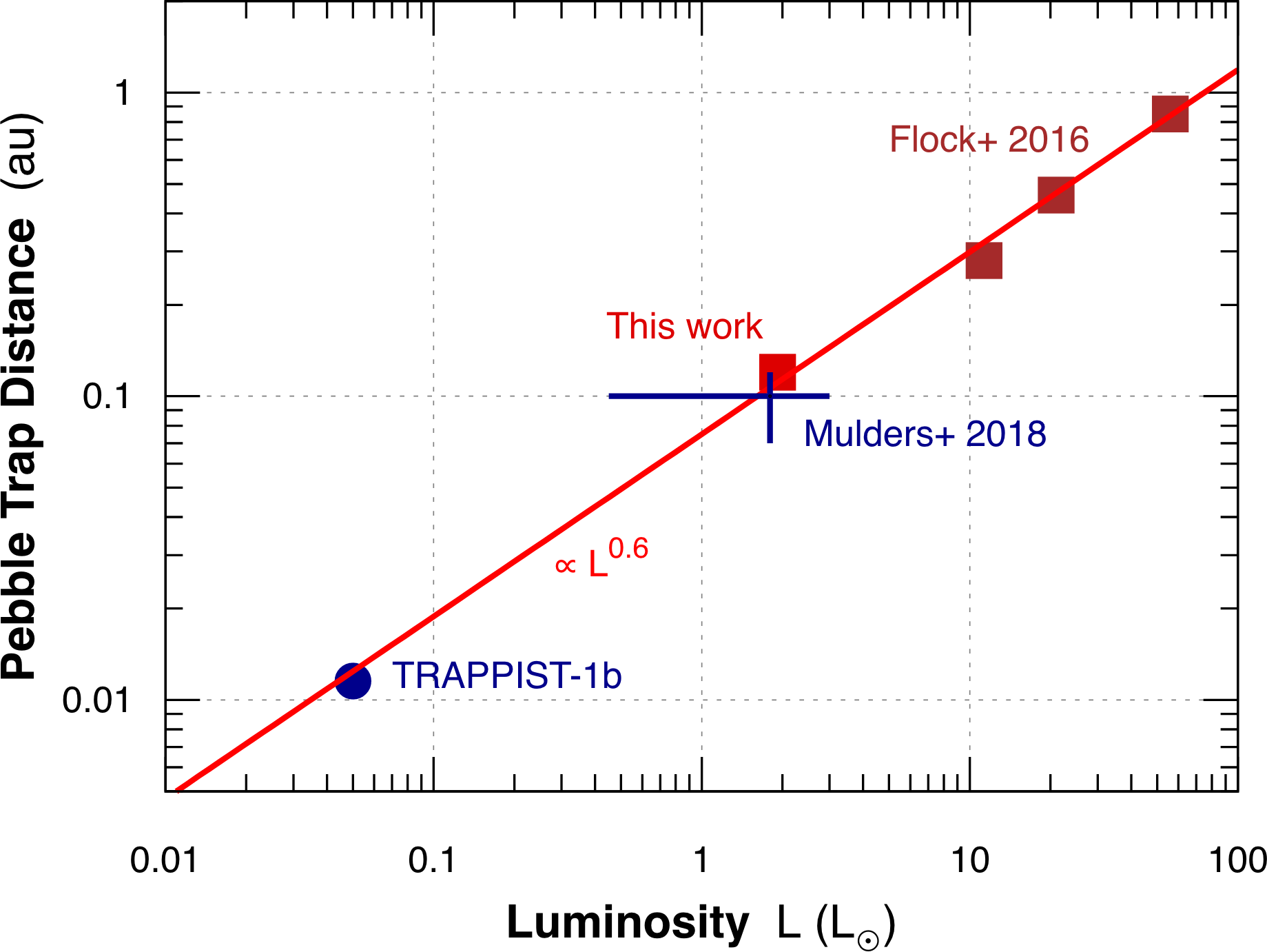
Figure 8: Relation between the pebble trap distance and the luminosity of the star. The leftmost red cross is from model MREF and the rest are from our previous work (Flock et al., 2016).

As with the silicate sublimation front, the snow line is determined by the stellar luminosity. Bitsch et al. (2015) show that the snow line can lie inside 1 au at accretion rates similar to those we consider. The snow line is significantly farther from the star in our models for two reasons. First, the stellar luminosity is about twice as great. Second, the opacity for starlight exceeds that for the disk’s own thermal emission, where Bitsch et al. (2015) had the reverse. Absorbing efficiently and re-emitting inefficiently makes the dust hotter at a given starlight flux, pushing the snow line outward.

5 Discussion

In this section we discuss the effects of viscous heating, the magnetic driven wind, and the stellar magnetic field on our model. We compare our results to previously found migration maps and other planet formation models. Finally, we report on the effect that eccentricity and resonant chains might have.

5.1 Viscously heated or passive disk

We have focused here on irradiated passive disks. Our similar radiation hydrodynamical models of disks around intermediate-mass young stars show little impact from accretion heating (Flock et al., 2016). However for T Tauri disks accretion is more important since the ratio of accretion flux to irradiation flux at the sublimation front varies roughly inversely with stellar luminosity. To examine whether accretion heating is important, in Fig. 9 we compare the passive irradiated disk with one heated only by accretion. Following Hubeny (1990) the accretion flux radiated from the disk surface is

$$F_{acc}=\frac{3}{8\pi}\dot{M}\Omega^{2}\left(1-\sqrt{\frac{R_{0}}{R}}\right)$$ (19)

using the corotation radius $R_{0}$. With the accretion power deposited in the interior, the midplane temperature is

$$T_{mid}=\left(\frac{\tau_{Z}F_{acc}}{\sigma_{b}}\right)^{1/4},$$ (20)

for vertical Rosseland mean optical depth $\tau_{Z}$. The midplane accretion temperature for the reference model’s surface density profile is the blue dashed line in Fig. 9.

Figure 9: Profile of the midplane temperature in model MREF (black line) and in the model heated only by accretion using the classical $\alpha$ prescription (blue dashed line). The dotted vertical lines indicate the edges of the dead zone in MREF (left) and the $\alpha$ model (right).

The accretion heating shifts the edge of the dead zone from 0.1 au to 0.26 au. However, in the passive model (solid line in Fig. 9) the annulus between these two radii is cool enough to remain MRI inactive. Furthermore, the turbulent surface layer or base of the magnetized wind, where the accretion power is deposited when the interior is inactive, has an optical depth comparable to or less than unity (Bai & Goodman, 2009; Béthune et al., 2017; Mori et al., 2019). According to Eq. 20 the accretion temperature at the base of the active layer is well below the irradiation temperature, so accretion heating is negligible. Thus, the accretion flow in the passive irradiated model does not significantly alter its temperature. Furthermore, for the purpose of Fig. 9 we ignore the dust sublimation; by speeding up cooling sublimation would act as a thermostat and limit the temperature to $T_{s}$, again bringing the temperatures close to those in the passive model. We also note that the accretion-heated disk is much colder than the passive disk inside  0.08 au, due to the low gas opacity. If both irradiation and accretion were included, the temperature here would be similar to the irradiation-only case.

In summary, the passive irradiated models accurately represent the thermal structure. However, accretion heating is important between the inner rim and the edge of the dead-zone for higher mass accretion rates $\rm\dot{M}\geq 10^{-8}$, pushing the edge of the dead zone and the planetary trap farther out. However, even in this case, we still expect that the first planetary core to form will be dry, since the dead-zone pebble trap always occurs at high temperatures of around 800K to 1000K.

5.2 Torque map comparison

One noticeable difference from previous models is the contribution of the entropy-related corotation torque. In our models this effect is slight, giving rise only to a small outward migration region that sits outside the pebble trap in Fig. 5. In previous studies for T Tauri systems that include a higher viscous heating (Coleman & Nelson, 2014; Bitsch et al., 2015), the outward migration zone extends to 5 au and beyond because of the steeper temperature gradient obtained in viscously heated disks. Following the previous discussion, we expect that the contribution from the entropy-related corotation torque in the dead zone should remain small in the absence of another source of heating.

5.3 Gap-opening mass

Equation 15 yields traditional gap-opening mass appropriate to viscous disks. However, if $\alpha_{DZ}$ takes the form of an external torque applied by magneto-centrifugally launching a wind from the disk surface, its character may be quite unlike a viscosity, influencing the gap-opening mass. In this case, where the disk midplane is laminar, the gap-opening mass is much lower (Rafikov, 2002; Dong et al., 2011; McNally et al., 2019), especially for the low values of $H/R$ in our models.

5.4 Exact shape and position of the inner rim

When the sublimation front is highly unresolved, the starlight is absorbed in the near face of the first dust-containing cell it meets, yet the heat is deposited uniformly through that cell, including its unlit interior and back side. Therefore the cell’s front side is cooler than it should be. Yet the front side is what we see in the infrared if the cell is optically thick. Thus, the disk’s thermal radiation appears at too long a wavelength and the front’s shape and position may be computed incorrectly. To resolve this issue, we developed a method that reduces the dust abundance smoothly across the sublimation front so that the transition from optically thin to thick is spatially resolved (Flock et al., 2016). This approach may become unnecessary in future when multiple grain compositions and sizes are included. A mix of species, each with its own sublimation temperature, naturally blurs the rim (Kama et al., 2009).

The rim’s location suffers from uncertainty because anything near the star that is opaque enough allows dust to survive within its shadow. Our models, which assume a very low gas opacity, should therefore be seen as producing an outermost limit with respect to the radial position of the rim. We note that the exact location of the pebble and planetary traps are influenced by the rim location and the location of the ionization transition. Furthermore, we expect the small grains in the dead zone to deplete quickly. Ueda et al. (2018) show that small grains grow efficiently in the dead zone, due to its weak turbulence, forming pebbles that drift inward quickly.

One set of parameters we have not varied is the stellar temperature, radius, and mass. These parameters affect the position of the inner rim and other features in the structure of the disk, and thus should be investigated in the future (Mulders et al., 2015).

5.5 Influence of stellar magnetic field on the rim shape

The star’s magnetic field could potentially disturb the disk near the sublimation front (Romanova et al., 2012). To determine whether our neglect of the stellar field is valid, we consider a dipole with strength of 1 kilogauss at the stellar surface (Johns-Krull, 2007). The field strength in the midplane at 0.1 au is 1.8 gauss. For our reference model MREF, the thermal pressure at the midplane in the same location is $\rm P_{th}=240dyn\,cm^{-2}$. The plasma beta is thus 1900. If it penetrated the disk’s plasma, a field of this strength would be important for driving MRI turbulence. Although we would not expect a very strong effect on the rim profile or height, which we investigated in our previous work (Flock et al., 2017), we note that the $\alpha_{MRI}=0.1$ value used in model M2 might be more realistic under these conditions.

5.6 Comparison with other planet formation models

Because our disk models produce both a pebble trap and a planet trap, our results in principle support both an in situ planet formation model based on the drift and concentration of pebbles which then form planets (Boley et al., 2014; Chatterjee & Tan, 2014) and a model based on the formation of planets farther from the star, which then migrate inward until they are halted at the planet trap (Izidoro et al., 2017, 2019). The migration model appears most able to explain the fact that some systems, such as Trappist I which contains seven terrestial planets around an M star (Gillon et al., 2016, 2017), are composed of planets in chains of mean motion resonances. In this model the planets migrate toward the inner edge of the protoplanetary disk until they are parked in resonant chains. Recent work suggests that many of these resonant chains can become unstable after the gas disk dissipates, explaining why most of the systems discovered by the Kepler mission are not in resonance (Izidoro et al., 2017, 2019; Lambrechts et al., 2019).

Without an inner disk edge and planet trap, migration would drive all planets into the central star, and resonant chains would not exist because planets could not pile up. Ormel et al. (2017) proposed that planetary cores form at the snow line and then migrate inward while continuing to grow via pebble accretion. It is noteworthy that the innermost Trappist-1 planet is located at around 0.01 au, which is roughly consistent with the inner edge of the dust disk if the luminosity was at least one order of magnitude higher than it is currently, as is expected for young, very low-mass stars (Laughlin & Bodenheimer, 1993).

5.7 Eccentricity effect on the torque

We assume an orbital eccentricity of zero when calculating the torque map. However, planets undergoing type I migration may have a small eccentricity value, for example due to being embedded in a turbulent region of the disk (Laughlin et al., 2004) or because multiple planets migrate together with a small separation. In such a case the outward migration zone would shrink since the corotation torque becomes weaker (Fendyke & Nelson, 2014; Coleman & Nelson, 2016). This could shift the planet traps even closer to the star, depending on the details of the density profile near the ionization transition zone. The shift is in the right direction to improve the fit to the occurrence rate of Kepler planets. In addition, if the turbulence is particularly vigorous, the outward migration zone located around 0.08 au may shrink, or disappear altogether if the eccentricity exceeds the disk aspect ratio of about 0.02. This will need to be examined in the future using radiation-MHD simulations of planets embedded in magnetized disks.

5.8 Effect of resonant chains

The innermost planet in a multiplanetary system could also be pushed nearer to the star by torques from the outer planets in the resonant chain (Carrera et al., 2018; Izidoro et al., 2019; Carrera et al., 2019). This might improve the agreement between the innermost planet position and the Kepler results of Mulders et al. (2018). Furthermore, multiplanetary systems tend to become unstable, leading to scattering and collisions among the planets once the disk has dispersed, which could explain the occurrence of super-Earths interior to any planet trap position (Izidoro et al., 2017, 2019).

6 Conclusion

We developed radiation hydrostatic models to describe the thermal and density structure of protoplanetary disks around T Tauri stars. The models are 2D and axisymmetric, and include stellar irradiation, dust and gas opacities, dust sublimation, and condensation. Magnetically driven accretion is modeled by means of a temperature-dependent kinematic viscosity. This dependence is chosen to capture the onset of magneto-rotational turbulence at temperatures around 900 K. The models are inflow-equilibrium solutions with radially constant mass accretion rates. All our models are for a typical young Sun-like star with parameters of $T_{*}=4300$K, $R_{*}=2.6\,R_{\sun}$, and $M_{*}=1.0\,M_{\sun}$. We examine disk mass accretion rates from $\rm\dot{M}=10^{-9}\,to\,10^{-8}M_{\sun}/yr$, and dust-to-gas mass ratios between $10^{-4}$ and $10^{-3}$, considering grains smaller than 10 $\rm\mu m$ that are responsible for absorbing incoming stellar radiation and reemitting it in the thermal infrared.

The computational domain spans the dust sublimation front and the water snow line. The resulting disk structure is approximately a scaled-down version of the Herbig disk models obtained by Flock et al. (2016):

• In our reference model the dust sublimation front occurs at around 0.08 au in the midplane, and curves out to around 0.15 au at an elevation angle of $Z/R=0.08$.

• The next feature outward after the sublimation front is a steep increase in density due to the drop in the ionization level and the corresponding drop in the accretion stress. Here at 0.13 au we find a robust local pressure maximum capable of trapping pebble-sized particles.

• Orbital migration torques calculated for embedded super-Earths indicate that type I migration halts at around 0.13 au. The planet migration trap lies close to the peak (from the Kepler survey) in the orbital distribution of the innermost planets in multiplanetary systems.

• The orbital period at the pebble trap in our reference model is 17 days. In a model with the dust abundance ten times lower, the pebble trap is shifted inward to an orbital period of 10 days.

• For all of our models, the snow line is located close to 1.6 au at the midplane, reaching 2 au at two scale heights above the midplane. This closely matches the peak in the occurrence rate of giant planets from radial velocity surveys.

We point out that our results can in principle support both of the leading planet formation scenarios. The disk structure we determined allows inward-drifting pebbles to accumulate and form planets at the pressure maximum a short distance outside the dust sublimation front. The model also allows planet formation to occur farther out in the disk, for example at the snow line, after which the planets migrate inward and become trapped beneath the inner rim formed by the dust sublimation front. In the future it will be important to test these findings using full 3D radiation-MHD simulations with embedded pebbles and planets, so the dynamics of these bodies can be computed within the context of the complex and turbulent flows present in the inner regions of protoplanetary disks.

Appendix A Orbital migration torque maps

We show torque maps for all remaining models in Fig. 10. They are directly comparable with the map for the reference model in Fig. 5.

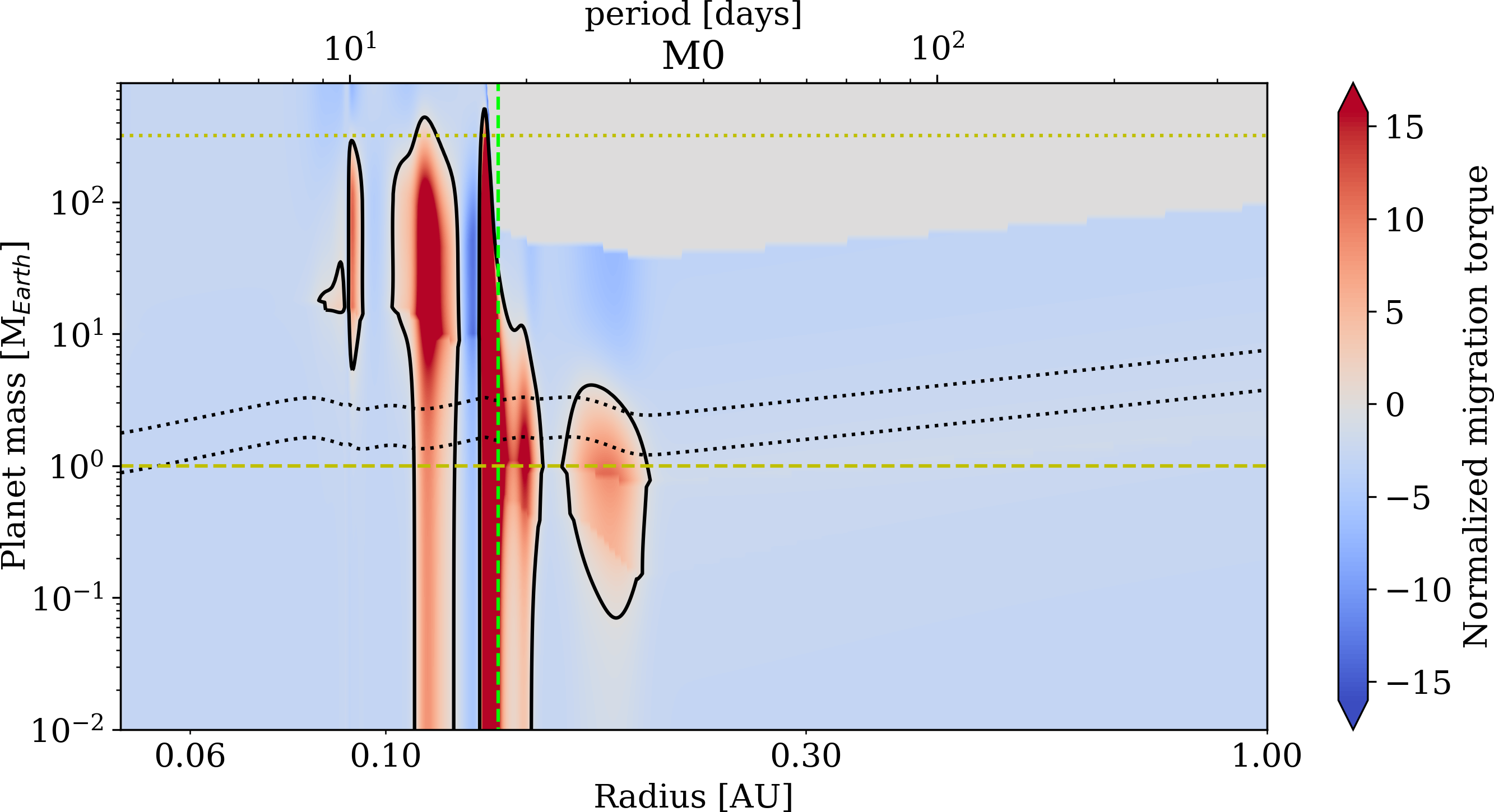
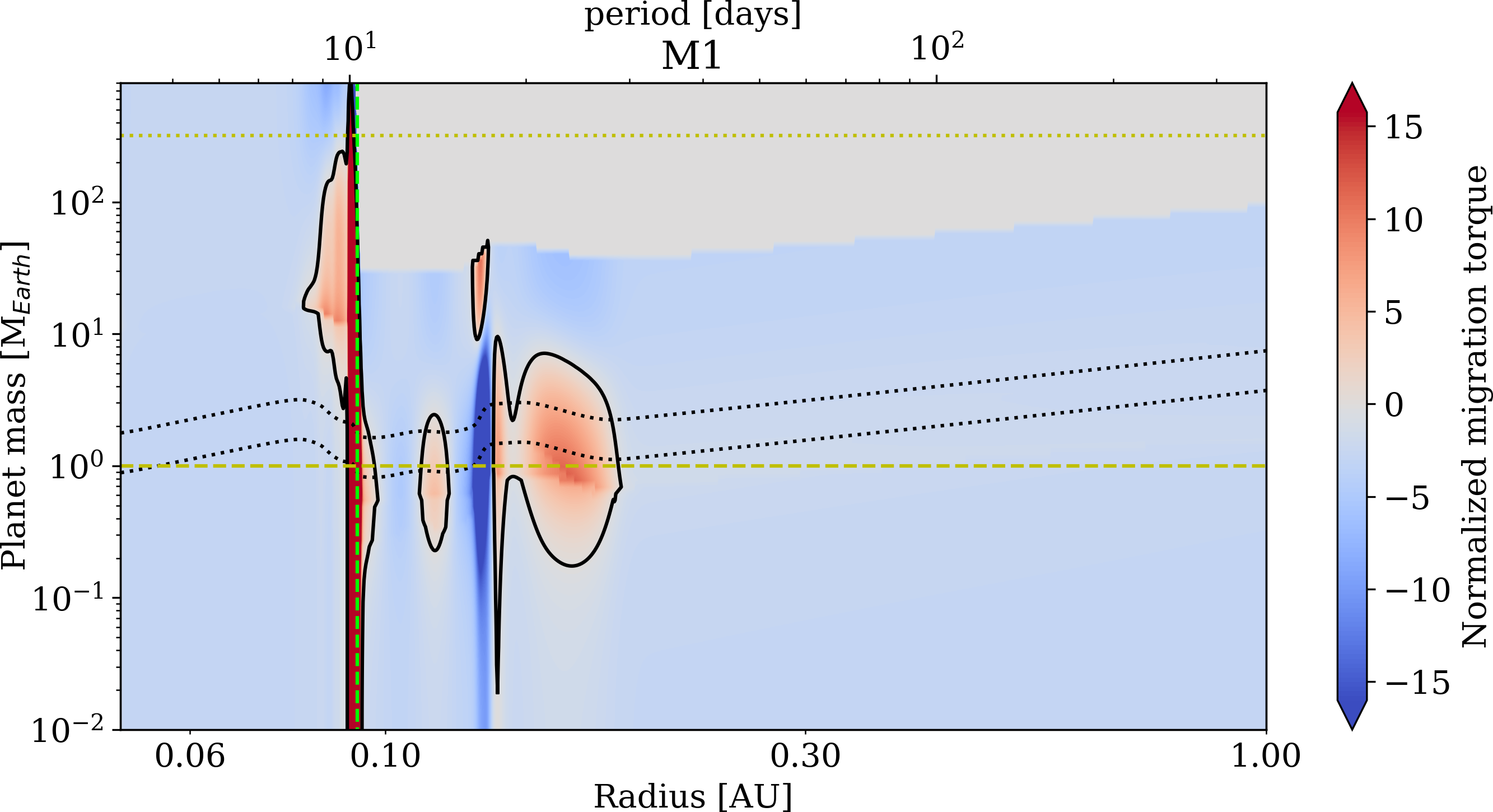
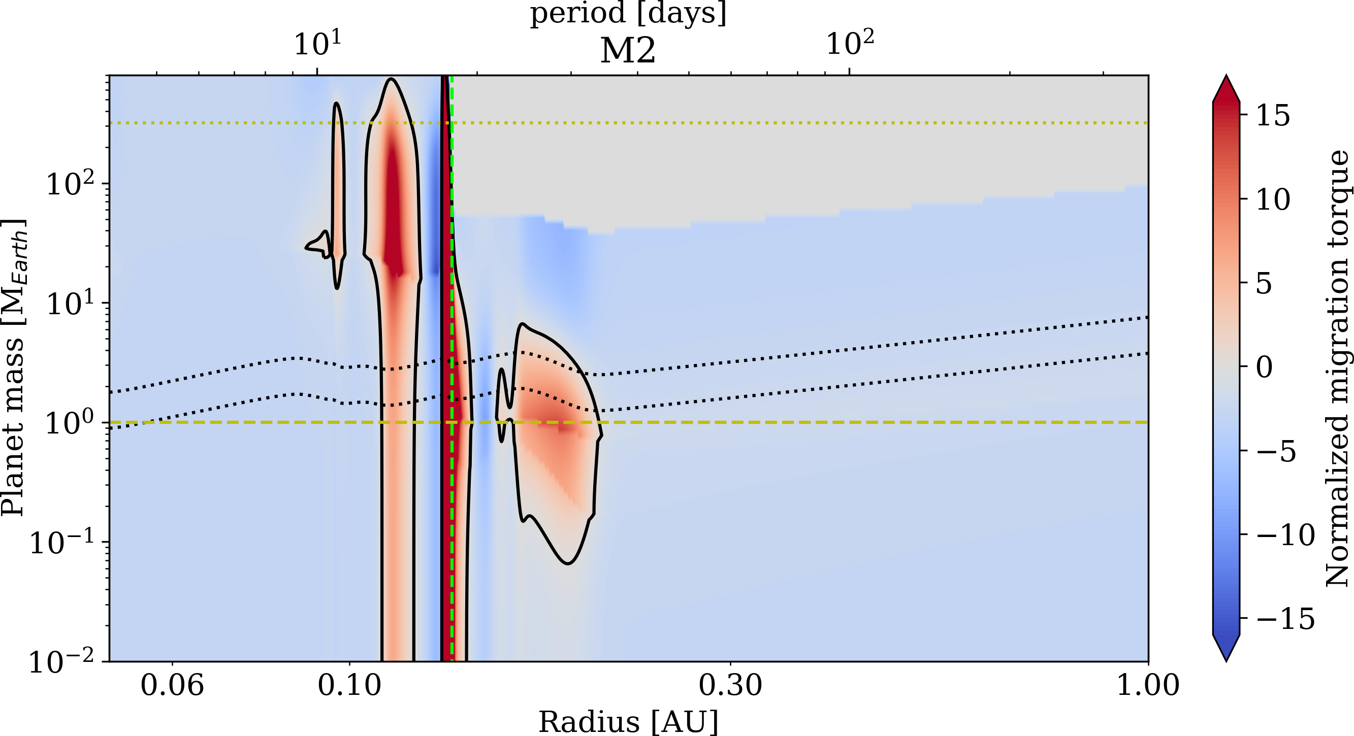
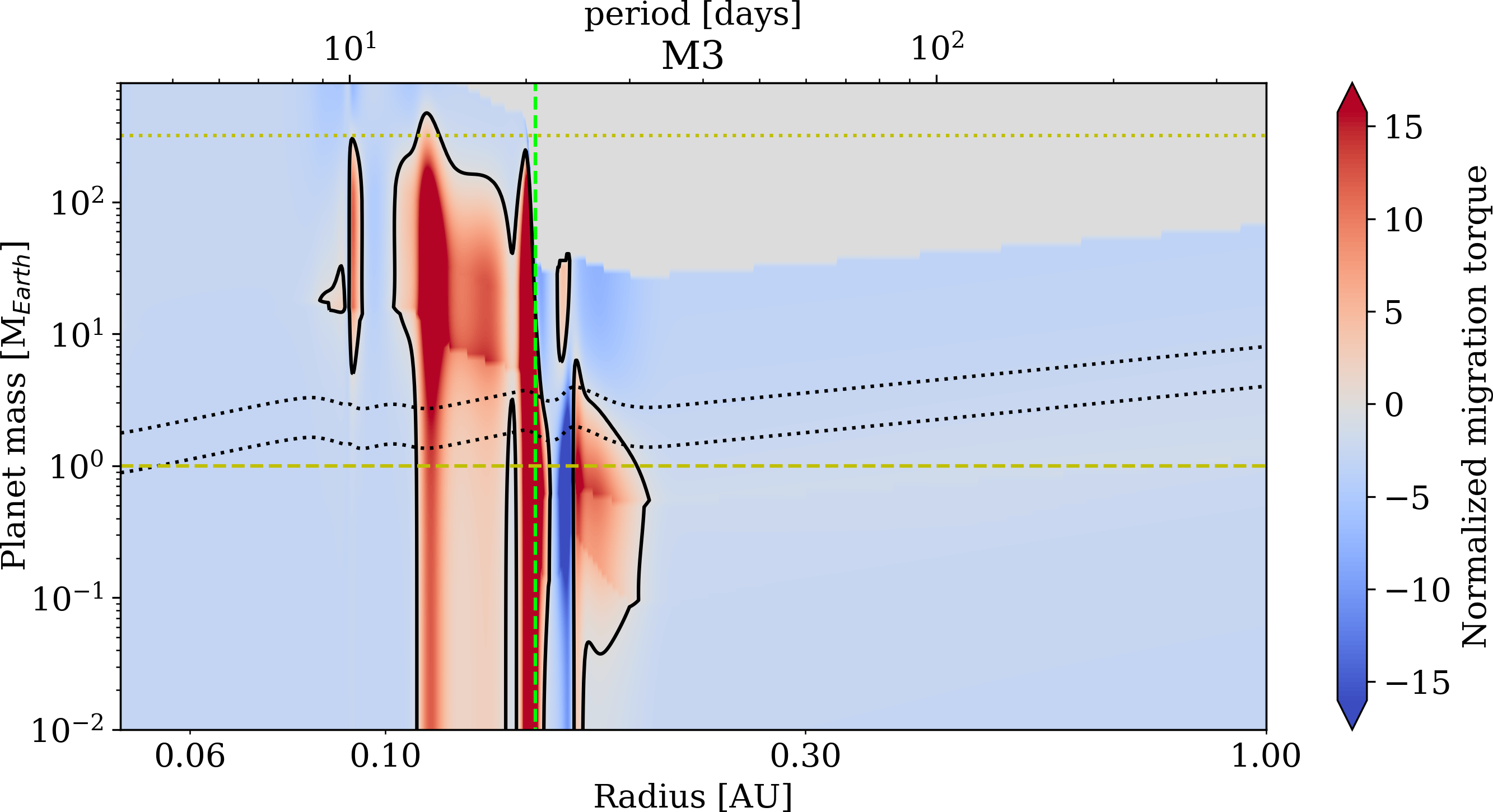
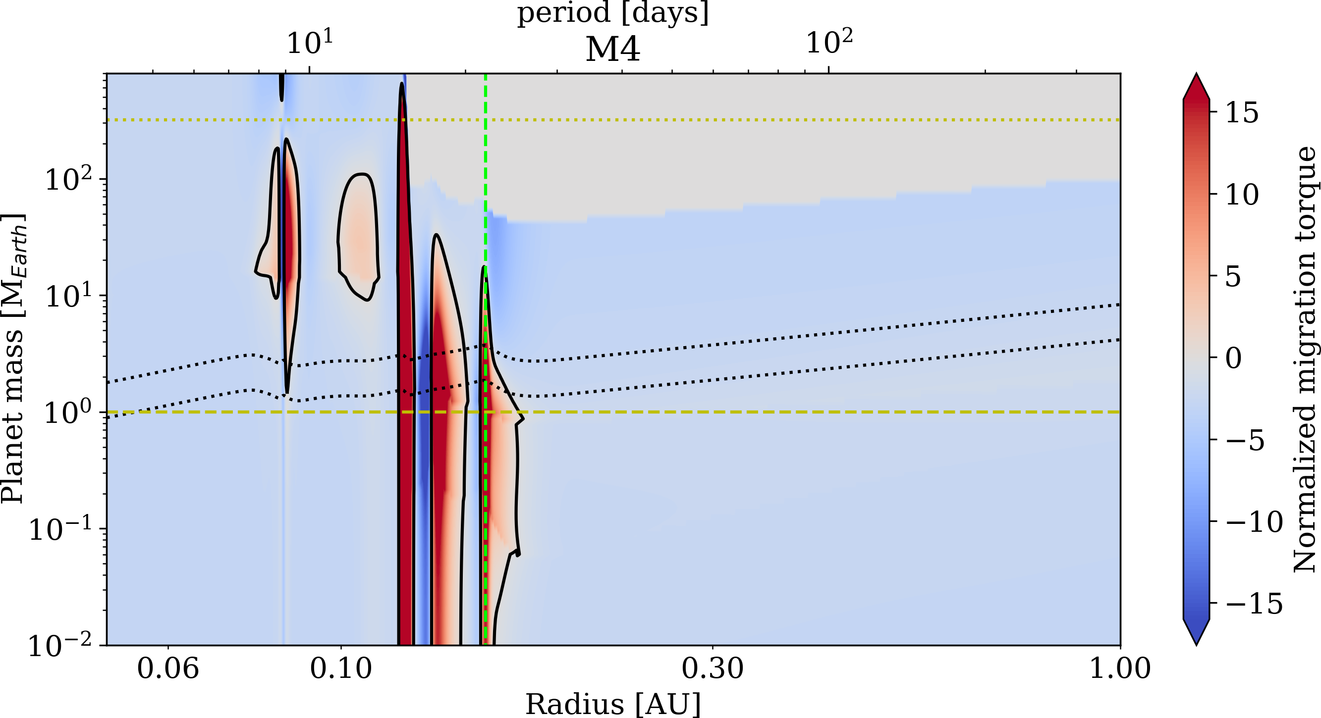
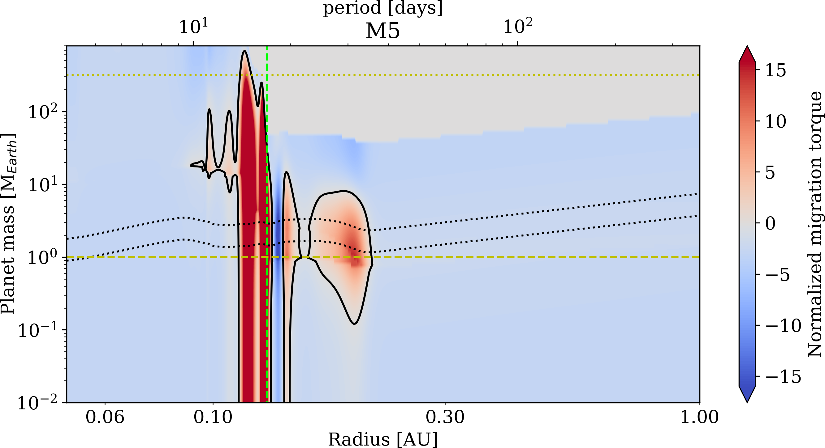
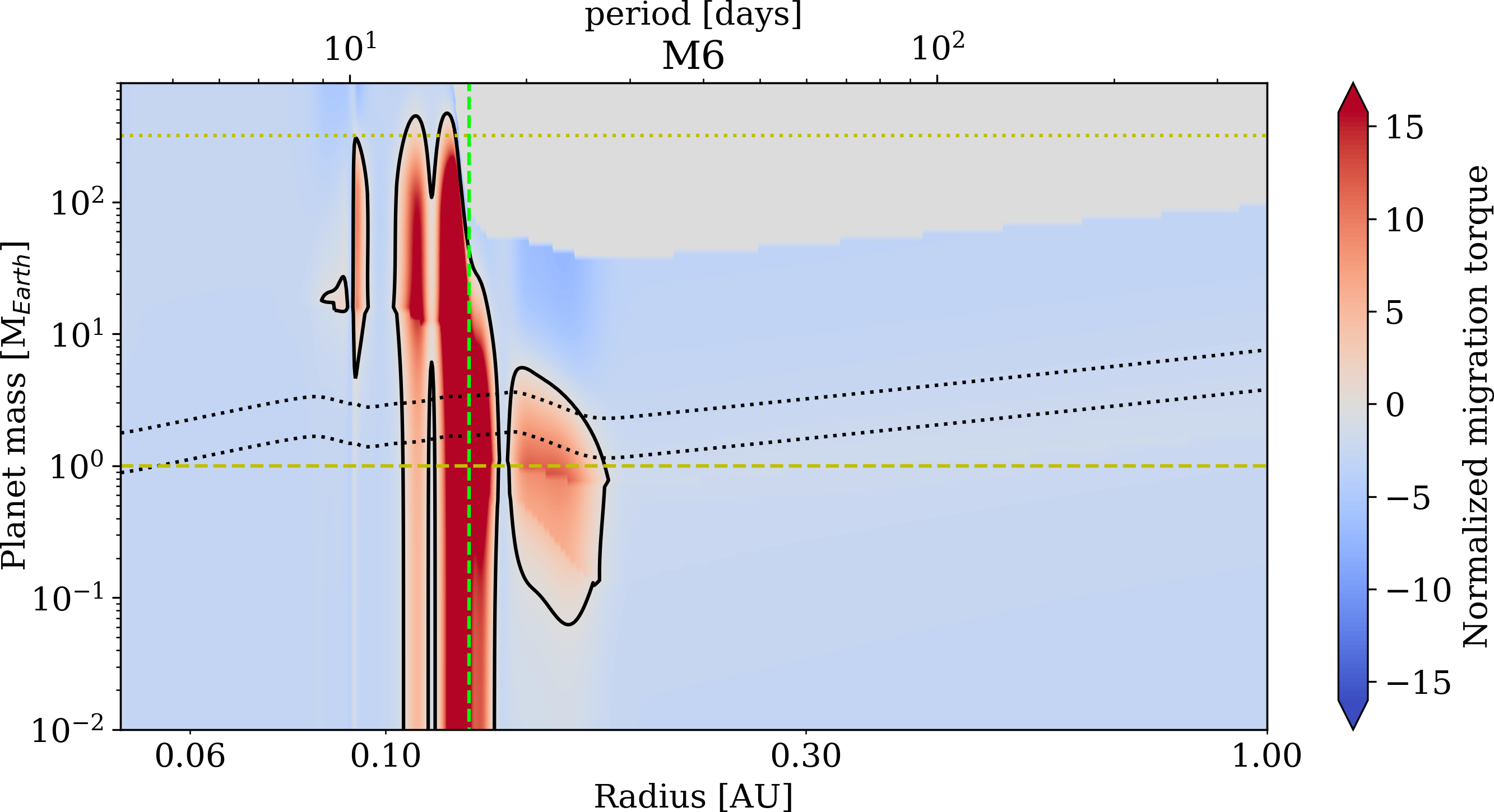
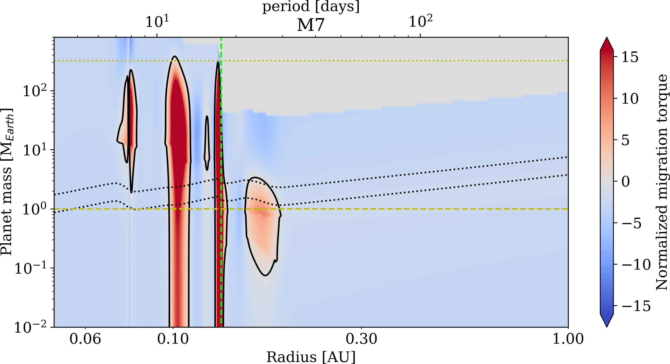
Figure 10: Torque maps for models M0 through M7.

Appendix B Opacity model

B.1 Gas opacity

In our previous work (Flock et al., 2016) we included a simple temperature- and pressure-independent gas opacity of $\rm\kappa_{gas}=10^{-4}cm^{2}g^{-1}$. For this new work, we make use of the more detailed gas opacities derived by Malygin et al. (2014). Figure 11 shows the Rosseland mean gas opacities.

Over the temperature and pressure regime of our model we derive a mean value of about $\rm\kappa_{gas}=10^{-5}cm^{2}g^{-1}$. For simplicity we assume the same gas opacity also for the irradiation. Future calculations of the detailed gas opacity including photochemistry are necessary to improve this step. A higher gas opacity could affect the rim shape and the temperature profile of the inner disk.

B.2 Dust opacity

To compute the dust opacity we used the tool MieX (Wolf & Voshchinnikov, 2004). We assumed silicate and carbon particles with radii between $\rm a_{min}=0.005\mu m$ and $\rm a_{max}=10\mu m$ and a grain size distribution having exponent $-3.5$. The particles are $62.5\%$ astrophysical silicate and $37.5\%$ graphite. The wavelength dependence of the dust opacity is plotted in Fig. 11.

From the wavelength-dependent opacity we determine the Planck mean using

$$\rm\kappa_{P}(T)=\frac{\int_{0}^{\infty}\kappa_{\nu}B(\nu,T)d\nu}{\int_{0}^{\infty}B(\nu,T)d\nu},$$ (21)

with the Planck function $\rm B(\nu,T)$. The frequency integral corresponds to a wavelength between 0.05 $\rm\mu m$ and 2 $\rm mm$. For the starlight color temperature $\rm T_{*}=4300\,K$, we determine two significant figures $\rm\kappa_{P}(T_{*})=1300cm^{2}g^{-1}$. For the sublimation front color temperature $\rm T_{s}=1500K$, we determine $\rm\kappa_{P}(T_{s})=700cm^{2}g^{-1}$.

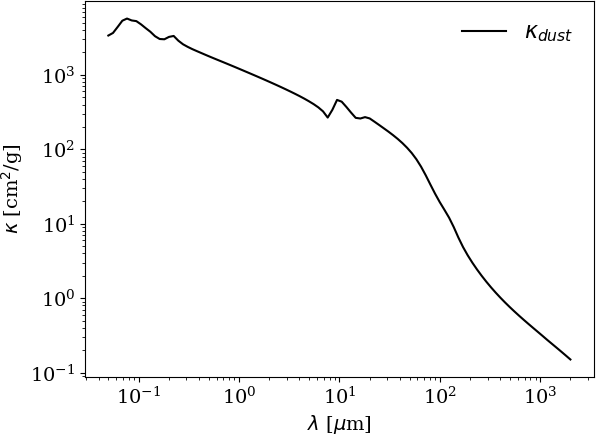
Figure 11: Top: Rosseland mean gas opacity vs. temperature and pressure (Malygin et al., 2014). The rectangle indicates the temperatures and pressures relevant for our model. Bottom: Total dust opacity per gram of dust over wavelength.

References

- Amard et al. (2019) Amard, L., Palacios, A., Charbonnel, C., et al. 2019, arXiv e-prints, arXiv:1905.08516
- Bai & Goodman (2009) Bai, X.-N. & Goodman, J. 2009, ApJ, 701, 737
- Batalha et al. (2013) Batalha, N. M., Rowe, J. F., Bryson, S. T., et al. 2013, ApJS, 204, 24
- Béthune et al. (2017) Béthune, W., Lesur, G., & Ferreira, J. 2017, A&A, 600, A75
- Birnstiel et al. (2012) Birnstiel, T., Klahr, H., & Ercolano, B. 2012, A&A, 539, A148
- Bitsch et al. (2015) Bitsch, B., Johansen, A., Lambrechts, M., & Morbidelli, A. 2015, A&A, 575, A28
- Bitsch & Kley (2011) Bitsch, B. & Kley, W. 2011, A&A, 536, A77
- Bitsch et al. (2018) Bitsch, B., Morbidelli, A., Johansen, A., et al. 2018, A&A, 612, A30
- Boley et al. (2014) Boley, A. C., Morris, M. A., & Ford, E. B. 2014, ApJ, 792, L27
- Brasser et al. (2018) Brasser, R., Matsumura, S., Muto, T., & Ida, S. 2018, ApJ, 864, L8
- Carrera et al. (2019) Carrera, D., Ford, E. B., & Izidoro, A. 2019, arXiv e-prints [arXiv:1903.02004]
- Carrera et al. (2018) Carrera, D., Ford, E. B., Izidoro, A., et al. 2018, ApJ, 866, 104
- Chatterjee & Tan (2014) Chatterjee, S. & Tan, J. C. 2014, ApJ, 780, 53
- Coleman & Nelson (2014) Coleman, G. A. L. & Nelson, R. P. 2014, MNRAS, 445, 479
- Coleman & Nelson (2016) Coleman, G. A. L. & Nelson, R. P. 2016, MNRAS, 460, 2779
- Crida & Bitsch (2017) Crida, A. & Bitsch, B. 2017, Icarus, 285, 145
- Crida et al. (2006) Crida, A., Morbidelli, A., & Masset, F. 2006, Icarus, 181, 587
- D’Antona & Mazzitelli (1994) D’Antona, F. & Mazzitelli, I. 1994, ApJS, 90, 467
- Dawson et al. (2015) Dawson, R. I., Chiang, E., & Lee, E. J. 2015, MNRAS, 453, 1471
- Dawson et al. (2016) Dawson, R. I., Lee, E. J., & Chiang, E. 2016, ApJ, 822, 54
- Desch & Turner (2015) Desch, S. J. & Turner, N. J. 2015, ApJ, 811, 156
- Dong et al. (2011) Dong, R., Rafikov, R. R., & Stone, J. M. 2011, ApJ, 741, 57
- Dr\każkowska & Alibert (2017) Dr\każkowska, J. & Alibert, Y. 2017, A&A, 608, A92
- Dullemond & Monnier (2010) Dullemond, C. P. & Monnier, J. D. 2010, ARA&A, 48, 205
- Fabrycky et al. (2014) Fabrycky, D. C., Lissauer, J. J., Ragozzine, D., et al. 2014, ApJ, 790, 146
- Faure & Nelson (2016) Faure, J. & Nelson, R. P. 2016, A&A, 586, A105
- Fendyke & Nelson (2014) Fendyke, S. M. & Nelson, R. P. 2014, MNRAS, 437, 96
- Fernandes et al. (2018) Fernandes, R. B., Mulders, G. D., Pascucci, I., Mordasini, C., & Emsenhuber, A. 2018, arXiv e-prints [arXiv:1812.05569]
- Flock et al. (2016) Flock, M., Fromang, S., Turner, N. J., & Benisty, M. 2016, ApJ, 827, 144
- Flock et al. (2017) Flock, M., Nelson, R. P., Turner, N. J., et al. 2017, ApJ, 850, 131
- Fogg & Nelson (2007) Fogg, M. J. & Nelson, R. P. 2007, A&A, 472, 1003
- Furlan et al. (2006) Furlan, E., Hartmann, L., Calvet, N., et al. 2006, ApJS, 165, 568
- Furlan et al. (2011) Furlan, E., Luhman, K. L., Espaillat, C., et al. 2011, ApJS, 195, 3
- Furlan et al. (2009) Furlan, E., Watson, D. M., McClure, M. K., et al. 2009, ApJ, 703, 1964
- Gillon et al. (2016) Gillon, M., Jehin, E., Lederer, S. M., et al. 2016, Nature, 533, 221
- Gillon et al. (2017) Gillon, M., Triaud, A. H. M. J., Demory, B.-O., et al. 2017, Nature, 542, 456
- Hubeny (1990) Hubeny, I. 1990, ApJ, 351, 632
- Ida & Lin (2010) Ida, S. & Lin, D. N. C. 2010, ApJ, 719, 810
- Isella & Natta (2005) Isella, A. & Natta, A. 2005, A&A, 438, 899
- Izidoro et al. (2019) Izidoro, A., Bitsch, B., Raymond, S. N., et al. 2019, arXiv e-prints [arXiv:1902.08772]
- Izidoro et al. (2017) Izidoro, A., Ogihara, M., Raymond, S. N., et al. 2017, MNRAS, 470, 1750
- Johns-Krull (2007) Johns-Krull, C. M. 2007, ApJ, 664, 975
- Kama et al. (2009) Kama, M., Min, M., & Dominik, C. 2009, A&A, 506, 1199
- Lambrechts et al. (2014) Lambrechts, M., Johansen, A., & Morbidelli, A. 2014, A&A, 572, A35
- Lambrechts et al. (2019) Lambrechts, M., Morbidelli, A., Jacobson, S. A., et al. 2019, arXiv e-prints [arXiv:1902.08694]
- Laughlin & Bodenheimer (1993) Laughlin, G. & Bodenheimer, P. 1993, ApJ, 403, 303
- Laughlin et al. (2004) Laughlin, G., Steinacker, A., & Adams, F. C. 2004, ApJ, 608, 489
- Lee & Chiang (2017) Lee, E. J. & Chiang, E. 2017, ApJ, 842, 40
- Levermore & Pomraning (1981) Levermore, C. D. & Pomraning, G. C. 1981, ApJ, 248, 321
- Lissauer et al. (2011) Lissauer, J. J., Ragozzine, D., Fabrycky, D. C., et al. 2011, ApJS, 197, 8
- Lyra & Umurhan (2019) Lyra, W. & Umurhan, O. M. 2019, PASP, 131, 072001
- Malygin et al. (2014) Malygin, M. G., Kuiper, R., Klahr, H., Dullemond, C. P., & Henning, T. 2014, A&A, 568, A91
- Manara et al. (2017) Manara, C. F., Testi, L., Herczeg, G. J., et al. 2017, A&A, 604, A127
- Masset et al. (2006) Masset, F. S., Morbidelli, A., Crida, A., & Ferreira, J. 2006, ApJ, 642, 478
- McNally et al. (2019) McNally, C. P., Nelson, R. P., Paardekooper, S.-J., & Benítez-Llambay, P. 2019, MNRAS, 484, 728
- Mori et al. (2019) Mori, S., Bai, X.-N., & Okuzumi, S. 2019, arXiv e-prints, arXiv:1901.06921
- Mulders et al. (2015) Mulders, G. D., Pascucci, I., & Apai, D. 2015, ApJ, 798, 112
- Mulders et al. (2018) Mulders, G. D., Pascucci, I., Apai, D., & Ciesla, F. J. 2018, AJ, 156, 24
- Oka et al. (2011) Oka, A., Nakamoto, T., & Ida, S. 2011, ApJ, 738, 141
- Ormel et al. (2017) Ormel, C. W., Liu, B., & Schoonenberg, D. 2017, A&A, 604, A1
- Paardekooper et al. (2011) Paardekooper, S.-J., Baruteau, C., & Kley, W. 2011, MNRAS, 410, 293
- Paardekooper & Papaloizou (2008) Paardekooper, S.-J. & Papaloizou, J. C. B. 2008, A&A, 485, 877
- Petigura et al. (2018) Petigura, E. A., Marcy, G. W., Winn, J. N., et al. 2018, AJ, 155, 89
- Pollack et al. (1994) Pollack, J. B., Hollenbach, D., Beckwith, S., et al. 1994, ApJ, 421, 615
- Rafikov (2002) Rafikov, R. R. 2002, ApJ, 572, 566
- Rice et al. (2012) Rice, W. K. M., Veljanoski, J., & Collier Cameron, A. 2012, MNRAS, 425, 2567
- Romanova et al. (2012) Romanova, M. M., Ustyugova, G. V., Koldoba, A. V., & Lovelace, R. V. E. 2012, MNRAS, 421, 63
- Ros & Johansen (2013) Ros, K. & Johansen, A. 2013, A&A, 552, A137
- Rosotti et al. (2019) Rosotti, G. P., Booth, R. A., Tazzari, M., et al. 2019, MNRAS, 486, L63
- Schoonenberg et al. (2018) Schoonenberg, D., Ormel, C. W., & Krijt, S. 2018, A&A, 620, A134
- Siess et al. (2002) Siess, L., Livio, M., & Lattanzio, J. 2002, ApJ, 570, 329
- Terquem & Papaloizou (2007) Terquem, C. & Papaloizou, J. C. B. 2007, ApJ, 654, 1110
- Thi et al. (2018) Thi, W. F., Lesur, G., Woitke, P., et al. 2018, ArXiv e-prints, arXiv:1811.08663
- Ueda et al. (2018) Ueda, T., Flock, M., & Okuzumi, S. 2018, arXiv e-prints [arXiv:1811.09756]
- Ward (1997) Ward, W. R. 1997, Icarus, 126, 261
- Wolf & Voshchinnikov (2004) Wolf, S. & Voshchinnikov, N. V. 2004, Computer Physics Communications, 162, 113
- Youdin (2011) Youdin, A. N. 2011, ApJ, 742, 38