Policy Optimization Through Approximate Importance Sampling

Abstract

Recent policy optimization approaches (Schulman et al., 2015a, 2017) have achieved substantial empirical successes by constructing new proxy optimization objectives. These proxy objectives allow stable and low variance policy learning, but require small policy updates to ensure that the proxy objective remains an accurate approximation of the target policy value. In this paper we derive an alternative objective that obtains the value of the target policy by applying importance sampling (IS). However, the basic importance sampled objective is not suitable for policy optimization, as it incurs too high variance in policy updates. We therefore introduce an approximation that allows us to directly trade-off the bias of approximation with the variance in policy updates. We show that our approximation unifies previously developed approaches and allows us to interpolate between them. We develop a practical algorithm by optimizing the introduced objective with proximal policy optimization techniques (Schulman et al., 2017). We also provide a theoretical analysis of the introduced policy optimization objective demonstrating bias-variance trade-off. We empirically demonstrate that the resulting algorithm improves upon state of the art on-policy policy optimization on continuous control benchmarks.

1 Introduction

Policy gradient algorithms have achieved significant successes in reinforcement learning problems. Especially in continuous action settings policy gradient based methods provided a major milestone in achieving good empirical performance (Lillicrap et al., 2015; Duan et al., 2016). Despite these results policy gradient approaches can still have significant drawbacks. The policy updates often suffer from high variance, which can result in requiring prohibitively large numbers of interactions with environment. Additionally, policy gradient algorithms require careful tuning of the update step size which can be difficult in practice.

Recent policy optimization algorithms (Schulman et al., 2015a, 2017) have led to substantially improved the sample efficiency by optimizing a biased surrogate objective that has low variance. Optimizing this objective has been shown to stabilize learning (Duan et al., 2016; Schulman et al., 2015a; Achiam et al., 2017). The bias incurred by using the surrogate objective can be controlled by restricting the divergence between the target and behavior policy. The algorithms derived in (Schulman et al., 2015a, 2017) perform small steps in policy space using the biased proxy objective.

In this paper, we derive a new policy optimization objective starting from the value of the target policy obtained through importance sampling (IS). Importance sampling provides an unbiased estimate of the target policy’s value using samples from the current policy. Unfortunately, the raw IS objective is a poor target for optimization as the variance of importance sampling can increase exponentially with the horizon. We therefore introduce an approximation that allows us to directly trade-off the bias of approximation with the variance in policy updates. We show that our approximation unifies the previous proxy optimization approaches with the pure importance sampling objective and allows us to interpolate between them. We demonstrate that the resulting algorithm significantly improves upon state of the art on-policy policy optimization on a number of continuous control benchmarks and exhibits more robustness to suboptimal choice of hyperparameters.

In addition to the empirical results, we also analyse the theoretical properties of the introduced policy optimization objective in terms of providing upper bounds on bias and variance. There are important gaps in our understanding of TRPO (Schulman et al., 2015a) and similar algorithms as only loose bounds on the introduced bias were provided. We also aim to analyse and extend the theory behind these algorithms by quantifying the exact error term for surrogate objective as opposed to merely providing an upper bound. The results we derive allow to obtain the results provided in several previous works as special cases, including Schulman et al. (2015a); Achiam et al. (2017); Gu et al. (2017). Additionally, in the supplementary material we demonstrate that various policy gradient theorems (Sutton et al., 1999; Silver et al., 2014; Ciosek & Whiteson, 2018) can be unified and proven by simply differentiating the equality we derive.

This paper is organized as follows. We establish the notation in the background section. We follow by presenting the related work and formerly obtained results. Next, we introduce a novel policy optimization algorithm interpolating between importance sampling and a previously used proxy policy optimization objective. We proceed by theoretical analysis of the introduced policy optimization objective and analyze its bias and variance. We conclude by presenting the empirical results achieved by the introduced algorithm on continuous control benchmarks. We provide implementation of the algorithm derived in this paper used to carry out experiments.

2 Background

We begin by estabilishing notation. We assume a standard MDP formulation $(S,A,p,r,\gamma),$ with $S$ the set of states; $A$ the set of actions; $p:S\times A\times S\rightarrow\mathbb{R}_{+}$ represents the transition model, where $p(s^{\prime}|s,a)$ is the probability of transitioning to state $s^{\prime}$ when $a$ is taken in $s$; $r:S\times A\rightarrow[-R_{max},R_{max}]$ is the reward function and $\gamma\in(0,1)$ is a discount factor. A policy $\pi:S\times A\rightarrow\mathbb{R}_{+}$ induces a Markov chain with transition matrix $P_{\pi}$, i.e $P_{\pi}(s^{\prime},s)=\int p(s^{\prime}|s,a)\pi(a|s)da$. We use $\tau$ to denote a state action trajectory $(s_{0},a_{0},s_{1},a_{1},\ldots)$. We use notation $\tau\sim\pi$ to denote that the trajectory is sampled by following policy $\pi$, i.e. $s_{0}\sim\mu_{0}(\cdot)$, $a_{t}\sim\pi(\cdot|s_{t})$ and $s_{t+1}\sim p(\cdot|s_{t},a_{t})$, where $\mu_{0}(\cdot)$ denotes the initial distribution over states. The value of a policy $\pi$ is defined by:

$$\eta(\pi)=\operatorname*{\mathbb{E}}_{\tau\sim\pi}\sum_{t\geq 0}\gamma^{t}r(s_{t},a_{t}).$$ (1)

By $\operatorname*{\mathbb{E}}_{\tau\sim\pi|s,a}$ we denote an expectation taken over the trajectories obtained by following policy $\pi$ that begin with state $s$ and action $a$, i.e. $\operatorname*{\mathbb{E}}_{\tau\sim\pi|s,a}\sum_{t\geq 0}\gamma^{t}f(s_{t},a_{t})=\operatorname*{\mathbb{E}}_{\tau\sim\pi}\big{[}\sum_{t\geq 0}\gamma^{t}f(s_{t},a_{t})|s_{0}=s,a_{0}=a\big{]}$. We use standard notation to denote the value function given state $s$, $V^{\pi}(s)=\operatorname*{\mathbb{E}}_{\tau\sim\pi}\big{[}\sum_{t\geq 0}\gamma^{t}r(s_{t},a_{t})|s_{0}=s\big{]}$, and similarly we denote state action value $Q^{\pi}(s,a)=\operatorname*{\mathbb{E}}_{\tau\sim\pi}\big{[}\sum_{t\geq 0}\gamma^{t}r(s_{t},a_{t})|s_{0}=s,a_{0}=a\big{]}$. The advantage of policy $\pi$ at state $s$ and action $a$ is defined as $A^{\pi}(s,a)=Q^{\pi}(s,a)-V^{\pi}(s)$. Given the initial distribution over states $\rho_{0}$, we denote normalized discounted state occupancy measure by $d^{\pi}=(1-\gamma)\sum_{t\geq 0}\gamma^{t}P_{\pi}^{t}\mu_{0}$, so it follows that $d^{\pi}(s)=(1-\gamma)\sum_{t\geq 0}\gamma^{t}p(s_{t}=s|s_{0}\sim\mu_{0})$. We have that $\frac{1}{1-\gamma}\operatorname*{\mathbb{E}}_{s\sim d^{\pi},a\sim\pi(\cdot|s)}f(s,a)=\operatorname*{\mathbb{E}}_{\tau\sim\pi}\sum_{t\geq 0}\gamma^{t}f(s_{t},a_{t})$, where RHS can be estimated by performing rollouts from policy $\pi$.

We use $\rho_{t}(s_{t},a_{t})=\frac{\tilde{\pi}(a_{t}|s_{t})}{\pi(a_{t}|s_{t})}$ to denote importance sampling ratios and $\rho_{0:t}(s_{0:t},a_{0:t})=\prod_{i=0}^{t}\frac{\tilde{\pi}(a_{i}|s_{i})}{\pi(a_{i}|s_{i})}$ to denote their product. Throughout the paper we use $\tilde{\pi}$ to denote the target policy we aim to optimize and $\pi$ the behavior policy that was used to gather the current batch of data. Lastly, we denote the total variation distance between two distributions $p$ and $q$ as $\mathbb{D}_{\mathcal{TV}}\big{(}p(\cdot)||q(\cdot)\big{)}:=\frac{1}{2}\int|p(x)-q(x)|dx$.

3 Prior work

In this section we state well-known results linking the value of target policy $\eta(\tilde{\pi})$ with the value of data gathering policy $\eta(\pi)$. Kakade & Langford (2002) establish the expression for the difference of values between two arbitrary policies $\tilde{\pi}$ and $\pi$. They show that for any two policies $\pi$ and $\tilde{\pi}$, the difference of values $\eta(\tilde{\pi})-\eta(\pi)$ can be expressed as:

$$\eta(\tilde{\pi})-\eta(\pi)=\frac{1}{1-\gamma}\operatorname*{\mathbb{E}}_{s\sim d^{\tilde{\pi}},a\sim\tilde{\pi}(\cdot|s)}A^{\pi}(s,a).$$ (2)

Note Equation (2) cannot be used directly for policy optimization as the RHS of Equation (2) requires samples from $d^{\tilde{\pi}}$, the discounted state occupancy measure of the target policy $\tilde{\pi}$. Following Kakade & Langford (2002); Schulman et al. (2015a), we can replace the occupancy measure $d^{\tilde{\pi}}$ with $d^{\pi}$ to define an approximation $L_{\pi}(\tilde{\pi})$:

$$L_{\pi}(\tilde{\pi})=\frac{1}{1-\gamma}\operatorname*{\mathbb{E}}_{s\sim d^{\pi},a\sim\tilde{\pi}(\cdot|s)}A^{\pi}(s,a),$$ (3)

where we have slightly departed from the notation in Schulman et al. (2015a), by using $L_{\pi}(\tilde{\pi})$ to denote the proxy for the difference $\eta(\tilde{\pi})-\eta(\pi)$ instead of the value $\eta(\tilde{\pi})$.

The quantity $L_{\pi}(\tilde{\pi})$ can be estimated in practice and forms a backbone for modern policy optimization algorithms (Schulman et al., 2015a, 2017). However, changing the occupancy measure in Equation (2) introduces error which needs to be quantified. Kakade & Langford (2002) provided a lower bound on the value of policy being a linear combination of a target policy and behavior policy, $\forall_{s\in S}\ \tilde{\pi}(\cdot|s)=(1-\alpha)\pi(\cdot|s)+\alpha\pi^{\prime}(\cdot|s)$. They demonstrate that given behavior policy $\pi$, target policy $\pi^{\prime}$, and their linear combination $\tilde{\pi}(\cdot|s):=(1-\alpha)\pi(\cdot|s)+\alpha\pi^{\prime}(\cdot|s)\ \forall s\in S$, the following bound holds for $\alpha\in[0,1]$:

$$\eta(\tilde{\pi})-\eta(\pi)\geq\alpha L_{\pi}(\pi^{\prime})-\frac{2\alpha^{2}\epsilon\gamma}{(1-\gamma)(1-\gamma(1-\alpha))},$$ (4)

where $\epsilon=\max_{s\in\mathcal{S}}|\operatorname*{\mathbb{E}}_{a\sim\tilde{\pi}}A^{\pi}(s,a)|$.

Schulman et al. (2015a) follow on these results by providing the bound that is valid for any policies $\tilde{\pi}$ and $\pi$:

$$\eta(\tilde{\pi})-\eta(\pi)\geq L_{\pi}(\tilde{\pi})-\frac{4\epsilon\gamma\Delta^{2}}{(1-\gamma)^{2}},$$ (5)

where we denote $\Delta=\max_{s\in S}\mathbb{D}_{\mathcal{TV}}\big{(}\pi(\cdot|s)||\tilde{\pi}(\cdot|s)\big{)}$ and $\epsilon=\max_{s\in\mathcal{S}}|\operatorname*{\mathbb{E}}_{a\sim\tilde{\pi}}A^{\pi}(s,a)|$. The practical version of the algorithm derived in Schulman et al. (2015a) resorts to maximising $L_{\pi}(\tilde{\pi})$ w.r.t. $\tilde{\pi}$ in a neighbourhood of $\pi$, as the authors note that the obtained bound is too loose for the practical use. Achiam et al. (2017) further improves the bound given Equation (5) by replacing maximum operator with expectation. They show that the for any policies $\tilde{\pi}$ and $\pi$ the following bound holds:

$$\eta(\tilde{\pi})-\eta(\pi)\geq L_{\pi}(\tilde{\pi})-\frac{2\epsilon\gamma\delta}{(1-\gamma)^{2}},$$ (6)

where we denote $\delta:=\operatorname*{\mathbb{E}}_{s\sim d^{\pi}}\mathbb{D}_{\mathcal{TV}}\big{(}\pi(\cdot|s)||\tilde{\pi}(\cdot|s)\big{)}$ and $\epsilon=\max_{s\in\mathcal{S}}|\operatorname*{\mathbb{E}}_{a\sim\tilde{\pi}(\cdot|s)}A^{\pi}(s,a)|$. The presented bounds indicate that $L_{\pi}(\tilde{\pi})$ becomes a good proxy for $\eta(\tilde{\pi})-\eta(\pi)$ when policies $\pi$ and $\tilde{\pi}$ are close in terms of some form of divergence. The benefit of introducing $L_{\pi}(\tilde{\pi})$ is that it provides a biased but low variance surrogate for $\eta(\tilde{\pi})-\eta(\pi)$. The bias can be controlled by restricting the proximity of $\tilde{\pi}$ and $\pi$. Algorithms optimizing $L_{\pi}(\tilde{\pi})$ subject to some constraints have seen substantial empirical success (Schulman et al., 2015a, 2017; Duan et al., 2016).

Importance sampling has a long history of begin applied in off-policy evaluation (Thomas & Brunskill, 2016; Precup et al., 2000) and also used in context of PAC bounds for both off-policy evaluation (Thomas et al., 2015b) and policy optimization (Thomas et al., 2015a). Metelli et al. (2018) optimize the value of the policy $\eta(\tilde{\pi})$ obtained via importance sampling while regularizing divergence between $\tilde{\pi}$ and $\pi$ to obtain low variance in the estimated value $\eta(\tilde{\pi})$. Lowering the variance of IS estimator has been considered for value function estimation from off-policy data (Mahmood & Sutton, 2015; Munos et al., 2016; Espeholt et al., 2018).

Multiple approaches employ replay buffer (Mnih et al., 2013) to learn state action value function (Silver et al., 2014; Fujimoto et al., 2018) to improve sample efficiency of learning. Although this approach can lead to good empirical performance (Duan et al., 2016) it can also suffer from stability and possibly diverge by simultaneously applying bootstraping, off-policy learning and function approximation (Sutton & Barto, 1998; van Hasselt et al., 2018). Additionally using replay buffer significantly complicates theoretical analysis as introduced biases in general depend on all policies supplying data to buffer. In this work we focus on a setting in which only data incoming from current policy $\pi$ is used to learn target policy $\tilde{\pi}$.

4 Approximate Importance Sampling

	$f(s_{0:t},a_{0:t})$	$\alpha_{t}$	bias	variance
IS	$\rho_{0:t}(s_{0:t},a_{0:t})A^{\pi}(s_{t},a_{t})$	$(1,1,\ldots,1)$	no	high
TRPO	$\frac{\tilde{\pi}(a_{t}|s_{t})}{\pi(a_{t}|s_{t})}A^{\pi}(s_{t},a_{t})$	$(0,0,\ldots,0,1)$	yes	low
PPO	$\min(\phi^{\omega}\big{(}\frac{\tilde{\pi}(a_{t}|s_{t})}{\pi(a_{t}|s_{t})}\big{)}A^{\pi}(s_{t},a_{t}),\frac{\tilde{\pi}(a_{t}|s_{t})}{\pi(a_{t}|s_{t})}A^{\pi}(s_{t},a_{t}))$	-	yes	low
This paper	$\min(\phi^{\omega}\big{(}\prod_{i=1}^{t}\big{(}\frac{\tilde{\pi}(a_{i}|s_{i})}{\pi(a_{i}|s_{i})}\big{)}^{\alpha_{t}^{i}}\big{)}A^{\pi}(s_{t},a_{t}),\prod_{i=1}^{t}\big{(}\frac{\tilde{\pi}(a_{i}|s_{i})}{\pi(a_{i}|s_{i})}\big{)}^{\alpha_{t}^{i}}A^{\pi}(s_{t},a_{t}))$	any $\alpha_{t}\in[0,1]^{t+1}$	depends on $\alpha_{t}$	depends on $\alpha_{t}$

Table 1: Comparison of various functions used to approximate the value of target policy, $\eta(\tilde{\pi})$. Importance sampling is unbiased, but introduces excessive variance. TRPO reduces the variance by truncating products of importance sampling ratios, but this introduces bias. PPO provides a stable optimization procedure to optimize $L_{\pi}(\tilde{\pi})$ in the proximity of $\pi$. Our objective allows to interpolate between TRPO and IS and in turn trade off bias and variance.

Recent policy optimization approaches (Schulman et al., 2015a, 2017) optimize the proxy objective $L_{\pi}(\tilde{\pi})$ by keeping $\tilde{\pi}$ in proximity of $\pi$ where $L_{\pi}(\tilde{\pi})$ remains an accurate approximation. Alternatively, the value of target policy $\eta(\tilde{\pi})$ can be obtained by applying importance sampling.

Given a function $f:S\times A\rightarrow\mathbb{R}$ and two policies $\tilde{\pi}$ and $\pi$, the expectation $\operatorname*{\mathbb{E}}_{\tau\sim\pi}\sum_{t\geq 0}\gamma^{t}f(s_{t},a_{t})$ can be estimated with the step-based IS estimator (Precup et al., 2000; Jiang & Li, 2016):

$$\operatorname*{\mathbb{E}}_{\tau\sim\tilde{\pi}}\sum_{t\geq 0}\gamma^{t}f(s_{t},a_{t})=\operatorname*{\mathbb{E}}_{\tau\sim\pi}\sum_{t\geq 0}\gamma^{t}\rho_{0:t}(s_{0:t},a_{0:t})f(s_{t},a_{t}),$$ (7)

By applying the equality from Equation (7) to change the discounted occupancy measure in the RHS of Equation (2) from $d^{\tilde{\pi}}$ to $d^{\pi}$, we get:

$$\eta(\tilde{\pi})-\eta(\pi)=\operatorname*{\mathbb{E}}_{\tau\sim\pi}\sum_{t\geq 0}\gamma^{t}\rho_{0:t}(s_{0:t},a_{0:t})A^{\pi}(s_{t},a_{t}).$$ (8)

The RHS of Equation (8) can be estimated with samples as the expectation is taken over trajectories coming from current behavior policy $\pi$. However, Equation (8) is not suitable for policy optimization algorithms as the variance of importance sampling ratio products $\rho_{0:t}(s_{0:t},a_{0:t})$ increases exponentially with the horizon (Jiang & Li, 2016; Munos et al., 2016). In this section we introduce an objective function akin to $L_{\pi}(\tilde{\pi})$ that allows to trade-off the bias of approximation with the variance in policy updates.

We begin with the observation that the definition of $L_{\pi}(\tilde{\pi})$ can be seen as approximating products of importance sampling weights $\rho_{0:t}(s_{0:t},a_{0:t})$ with only the last term, $\rho_{0:t}(s_{0:t},a_{0:t})\approx\frac{\tilde{\pi}(a_{t}|s_{t})}{\pi(a_{t}|s_{t})}$. This approximation significantly reduces variance, but also introduces bias. Thus TRPO defines:

$$f^{TRPO}(s_{0:t},a_{0:t}):=\frac{\tilde{\pi}(a_{t}|s_{t})}{\pi(a_{t}|s_{t})}A^{\pi}(s_{t},a_{t}),$$ (9)

while the IS estimator defines:

$$f^{IS}(s_{0:t},a_{0:t}):=\rho_{0:t}(s_{0:t},a_{0:t})A^{\pi}(s_{t},a_{t}).$$ (10)

In both cases, $\eta(\tilde{\pi})-\eta(\pi)$ is then estimated by the expectation $\operatorname*{\mathbb{E}}_{\tau\sim\pi}\sum_{t\geq 0}\gamma^{t}f(s_{0:t},a_{0:t})$. This can be seen as resorting to two extremes: constructing a biased estimator with low variance or an unbiased estimator with high variance. To unify these approaches and interpolate between them we introduce the following function $f^{\alpha}$:

$$f^{\alpha}(s_{0:t},a_{0:t}):=\prod_{i=1}^{t}\Bigg{(}\frac{\tilde{\pi}(a_{i}|s_{i})}{\pi(a_{i}|s_{i})}\Bigg{)}^{\alpha_{t}^{i}}A^{\pi}(s_{t},a_{t}),$$ (11)

where $\alpha_{t}$ are vectors of length $t+1$ with coordinates $\alpha^{i}_{t}\in[0,1]$. Using Equation (11) allows us to construct the following approximation of $\eta(\tilde{\pi})-\eta(\pi)$:

$$L_{\pi}^{\alpha}(\tilde{\pi})=\operatorname*{\mathbb{E}}_{\tau\sim\pi}\sum_{t\geq 0}\gamma^{t}\prod_{i=1}^{t}\Bigg{(}\frac{\tilde{\pi}(a_{i}|s_{i})}{\pi(a_{i}|s_{i})}\Bigg{)}^{\alpha_{t}^{i}}A^{\pi}(s_{t},a_{t}).$$ (12)

Note that using $\alpha_{t}=(0,0,\ldots,0,1)$, $\forall t\geq 0$ corresponds to definition of $L_{\pi}(\tilde{\pi})$ and using $\alpha_{t}=(1,1,\ldots,1)$, $\forall t\geq 0$ recovers importance sampling. Intermediate values of $\alpha_{t}$ will trade off bias and variance. To see this we take the weighted power mean of $\rho_{t}(s_{t},a_{t})=\frac{\tilde{\pi}(a_{t}|s_{t})}{\pi(a_{t}|s_{t})}$ and 1 (i.e. $\tilde{\pi}(a_{t}|s_{t})\approx\pi(a_{t}|s_{t}))$ with respect to weight $\alpha_{t}^{i}$ so that

$$\hat{\rho}_{t}(s_{t},a_{t})=\rho_{t}(s_{t},a_{t})^{\alpha_{t}^{i}}\cdot 1^{(1-\alpha_{t}^{i})}=\rho_{t}(s_{t},a_{t})^{\alpha_{t}^{i}},$$

for all $t$. Hence,

$$\rho_{0:t}^{\alpha_{t}}(s_{0:t},a_{0:t}):=\prod_{i=1}^{t}\Bigg{(}\frac{\tilde{\pi}(a_{i}|s_{i})}{\pi(a_{i}|s_{i})}\Bigg{)}^{\alpha_{t}^{i}},$$ (13)

which leads to the definition of function $f^{\alpha}$ in Equation (11). Note that when $\alpha\rightarrow 0$, $f^{\alpha}(s_{0:t},a_{0:t})$ converges to a constant independent of $\tilde{\pi}$. This gives an estimator with large bias, but no variance. In fact, when $\alpha_{t}=(0,0,\ldots,0)$ for every $t\geq 0$ then

$$\operatorname*{\mathbb{E}}_{a_{t}\sim\pi(\cdot|s_{t})}f^{\alpha_{t}}(s_{0:t},a_{0:t})=\operatorname*{\mathbb{E}}_{a_{t}\sim\pi(\cdot|s_{t})}A^{\pi}(s_{t},a_{t})=0.$$ (14)

Using $\prod_{i=1}^{t}\big{(}\frac{\tilde{\pi}(a_{i}|s_{i})}{\pi(a_{i}|s_{i})}\big{)}^{\alpha_{t}^{i}}=e^{\sum_{i=1}^{t}\alpha_{t}^{i}\log\rho_{i}(s_{i},a_{i})}$ can be also viewed as temperature smoothing (Kirkpatrick et al., 1983) with temperatures $T_{i}=(\alpha_{t}^{i})^{-1}$. High temperatures cause terms $e^{\frac{\log\rho_{i}(s_{i},a_{i})}{T_{i}}}$ to be uniform and do not influence policy optimization.

To obtain further insights we analyse the gradient of $f^{\alpha_{t}}(s_{0:t},a_{0:t})$ with respect to the parameters of policy $\tilde{\pi}$:

$$\nabla f^{\alpha_{t}}(s_{0:t},a_{0:t})=\nabla e^{\sum_{i=0}^{t}\alpha_{t}^{i}\log\frac{\tilde{\pi}(a_{i}|s_{i})}{\pi(a_{i}|s_{i})}}A^{\pi}(s_{t},a_{t})$$

$$=e^{\sum_{i=0}^{t}\alpha_{t}^{i}\log\frac{\tilde{\pi}(a_{i}|s_{i})}{\pi(a_{i}|s_{i})}}\nabla\sum_{i=0}^{t}\alpha_{t}^{i}\log\frac{\tilde{\pi}(a_{i}|s_{i})}{\pi(a_{i}|s_{i})}A^{\pi}(s_{t},a_{t})$$

$$=\prod_{i=0}^{t}\rho_{i}(s_{i},a_{i})^{\alpha_{t}^{i}}\sum_{i=0}^{t}\alpha_{t}^{i}\frac{\pi(a_{i}|s_{i})}{\tilde{\pi}(a_{i}|s_{i})}\nabla\tilde{\pi}(a_{i}|s_{i})A^{\pi}(s_{t},a_{t}).$$ (15)

Since importance sampling ratios $\rho_{t}(s_{t})=1$ when $\tilde{\pi}=\pi$, evaluating the gradient $\nabla f^{\alpha_{t}}(s_{1:t},a_{1:t})$ at $\tilde{\pi}=\pi$ results in

$$\nabla f^{\alpha}(s_{0:t},a_{0:t})\Big{|}_{\tilde{\pi}=\pi}=\sum_{i=0}^{t}\alpha_{t}^{i}\nabla\tilde{\pi}(a_{i}|s_{i})A^{\pi}(s_{t},a_{t}).$$ (16)

As the expectation on RHS of Equation (12) is taken over trajectories from policy $\pi$ which does not depend on $\tilde{\pi}$, the gradient of the objective $L_{\pi}^{\alpha}(\tilde{\pi})$ evaluated at $\tilde{\pi}=\pi$ reads

$$\nabla L_{\pi}^{\alpha}(\tilde{\pi})\Big{|}_{\tilde{\pi}=\pi}=\operatorname*{\mathbb{E}}_{\tau\sim\pi}\sum_{t\geq 0}\gamma^{t}\sum_{i=0}^{t}\alpha_{t}^{i}\nabla\tilde{\pi}(a_{i}|s_{i})A^{\pi}(s_{t},a_{t}),$$ (17)

which can be rewritten as:

$$\nabla L_{\pi}^{\alpha}(\tilde{\pi})\Big{|}_{\tilde{\pi}=\pi}=\operatorname*{\mathbb{E}}_{\tau\sim\pi}\sum_{t\geq 0}\gamma^{t}\nabla\tilde{\pi}(a_{t}|s_{t})\sum_{i\geq t}\gamma^{i}\alpha^{t}_{i}A^{\pi}(s_{i},a_{i}).$$ (18)

Since we have that the telescopic sum $\sum_{i=t}^{T}\gamma^{i}A^{\pi}(s_{t},a_{t})=\sum_{i=t}^{T}\gamma^{i}r(s_{t},a_{t})+\gamma^{T+1}V(s_{T+1})-\gamma^{t}V^{\pi}(s_{t})$, in the case where $\tilde{\pi}=\pi$ the introduced weighting by $\alpha_{t}$ can be viewed as interpolating between using Monte Carlo returns and value function $V^{\pi}(s_{t})$ to estimate the returns for policy gradient. Also, note that in the case $\tilde{\pi}=\pi$, we have that $\nabla L_{\pi}^{\alpha}(\tilde{\pi})\big{|}_{\tilde{\pi}=\pi}=\nabla\eta(\tilde{\pi})|_{\tilde{\pi}=\pi}$ for any selection of $\alpha_{t}$. We extend this reasoning to a setting in which $\tilde{\pi}\neq\pi$.

Smoothing by $\alpha_{t}$ modifies the policy optimization target $L^{\alpha}_{\pi}(\tilde{\pi})$. During policy optimization we also need to consider the domain of policy $\tilde{\pi}$ over which we optimize as optimization can attempt to set individual importance sampling ratios $\rho_{t}$ to extreme values. Hence we are still required to constrain the divergence $\mathbb{D}_{\mathcal{TV}}(\pi(\cdot|s)||\tilde{\pi}(\cdot|s))$ during optimization to prevent $\tilde{\pi}$ from diverging. To optimize $L_{\pi}^{\alpha}(\tilde{\pi})$ in a stable manner we adopt the clipping scheme from Schulman et al. (2017). We clip the values of $\prod_{i=1}^{t}\big{(}\frac{\tilde{\pi}(a_{i}|s_{i})}{\pi(a_{i}|s_{i})}\big{)}^{\alpha_{t}^{i}}$ to be within the range of $(1-\omega,1+\omega)$ and take the minimum with $f^{\alpha}(s_{0:t},a_{0:t})$ to ensure the resulting function is a lower bound to $f^{\alpha}(s_{0:t},a_{0:t})$. We view employing clipping as obtaining an approximate solution to the constrained optimization problem $\max_{\tilde{\pi}}L^{\alpha}_{\pi}(\tilde{\pi})$ s.t. $\operatorname*{\mathbb{E}}_{\tau\sim\pi}\mathbb{D}_{\mathcal{TV}}(\pi(\cdot|s)||\tilde{\pi}(\cdot|s))<\epsilon$ which is necessary to execute optimization in a practical setting (Schulman et al., 2017). While KL regularization can be used for this purpose, we select clipping as it is reported to yield better empirical performance (Schulman et al., 2017). This results in the following definition of $f^{\alpha}_{\phi^{\omega}}(s_{0:t},a_{0:t})$:

$$f^{\alpha}_{\phi^{\omega}}(s_{0:t},a_{0:t})=\min\big{[} \phi^{\omega}(\hat{\rho}_{0:t}^{\alpha_{t}})A^{\pi}(s_{t},a_{t}),f^{\alpha}(s_{0:t},a_{0;t})\big{]},$$ (19)

where $\phi^{\omega}$ denotes a clipping function with the range of $(1-\omega,1+\omega)$. Next, the corresponding policy optimization objective $L_{\pi}^{\alpha,\phi^{\omega}}$ is defined as

$$L_{\pi}^{\alpha,\phi^{\omega}}(\tilde{\pi})=\operatorname*{\mathbb{E}}_{\tau\sim\pi}\sum_{t\geq 0}\gamma^{t}f^{\alpha_{t}}_{\phi^{\omega}}(s_{0:t},a_{0:t}).$$ (20)

To obtain a practical algorithm we approximate $\nabla L_{\pi}^{\alpha,\phi^{\omega}}(\tilde{\pi})$ with subsampled transitions. We collect the set of transitions $\{(s_{t},a_{t},r_{t},s_{t+1})\}_{t=1}^{T}$ we subsample a minibatch of timesteps $B$, and approximate the gradient $\nabla L_{\pi}^{\alpha,\phi^{\omega}}(\tilde{\pi})\approx|B|^{-1}\sum_{t\in B}\gamma^{t}\nabla f^{\alpha}_{\phi^{\omega}}(s_{0:t},a_{0:t})$. We use Generalized Advantage Estimation (Schulman et al., 2015b) to approximate the advantage function $A^{\pi}(s_{t},a_{t})$ with $\hat{A}^{\pi}(s_{t},a_{t})$. As the derived algorithm performs approximate importance sampling, we call it Approximate IS Policy Optimization. The resulting policy optimization procedure is summarized as Algorithm 1. We provide comparison of Approximate IS Policy Optimization with existing policy optimization approaches in Table 1.

Note that in general we face three sources of possible bias in updates of policy $\tilde{\pi}$ incoming from: (i) learning approximate critic $\hat{A}^{\pi}(s,a)$ using function approximation and bootstraping to lower the variance of policy updates (Schulman et al., 2015b; Tomczak et al., 2019), (ii) clipping applied to define $f^{\alpha}_{\phi^{\omega}}(s_{0:t},a_{0:t})$ to prevent individual importance weights $\rho_{t}$ from exploding during optimization and (iii) bias due to use of approximate occupancy measure $d^{\pi}$. PPO can control bias (i) by adjusting the $\lambda$ parameter in GAE critic and can control bias (ii) by increasing the clip value $\omega$ or reducing the number of optimization steps to learn policy $\tilde{\pi}$. However, PPO cannot correct for the bias incoming from employing $d^{\pi}$ as an occupancy measure. As importance sampling ratios are multiplied this type of bias can increase exponentially even if $\pi$ and $\tilde{\pi}$ remain close. The approach we develop enables us to control bias of type (iii) by adjusting $\alpha_{t}$. Therefore Approximate IS Policy Optimization can trade-off total bias in policy updates with their variance.

5 Theoretical Analysis

We begin by presenting theoretical analysis of the quality of the introduced estimator $L_{\pi}^{\alpha}(\tilde{\pi})$ in terms of providing upper bounds on a bias and variance on its estimator. We defer all proofs and discussion of assumptions of the subsequent results to the Appendix. We drop the dependency on the $s_{0:t}$ and $a_{0:t}$ when it is clear from the context. We first analyse the properties of random variable $\hat{L}_{\pi}^{\alpha}(\tilde{\pi}):=\sum_{t\geq 0}\gamma^{t}\rho_{0:t}^{\alpha_{t}}(s_{0:t},a_{0:t})A^{\pi}(s_{t},a_{t})$. We begin with the following Lemma providing the upper bound on $\mathbb{V}[\hat{L}_{\pi}^{\alpha}(\tilde{\pi})]$ in terms of norm $\left\lVert\alpha_{t}\right\rVert_{1}$.

Lemma 1.

Consider truncated horizon estimator defined by $\hat{L}_{\pi,T}^{\alpha}(\tilde{\pi}):=\sum_{t=0}^{T}\gamma^{t}\rho_{0:t}^{\alpha_{t}}(s_{0:t},a_{0:t})A^{\pi}(s_{t},a_{t})$. Assume that $\forall_{s\in\mathcal{S},a\in\mathcal{A}}\ \frac{\tilde{\pi}(a|s)}{\pi(a|s)}<C_{\rho}$. The variance $\mathbb{V}_{\tau\sim\pi}[L_{\pi,T}^{\alpha}(\tilde{\pi})]$ is upper bounded as

$$\operatorname*{\mathbb{V}}_{\tau\sim\pi}[L_{\pi,T}^{\alpha}(\tilde{\pi})]\leq\frac{1-\gamma^{T+1}}{1-\gamma}\epsilon^{2}\sum_{t=0}^{T}\gamma^{t}C_{\rho}^{2\left\lVert\alpha_{t}\right\rVert_{1}},$$ (21)

where $\epsilon=\max_{s\in\mathcal{S},a\in\mathcal{A}}|A^{\pi}(s,a)|$.

The significance of Lemma 1 is that once sparse vectors $\alpha_{t}$ with uniformly bounded number of non-zero components $K$ are employed we have that $\forall t\geq 0\ \left\lVert\alpha_{t}\right\rVert_{1}\leq K$ and the variance $\operatorname*{\mathbb{V}}_{\tau\sim\pi}[L_{\pi,T}^{\alpha}(\tilde{\pi})]$ is guaranteed to be finite and uniformly bounded by $\frac{\epsilon^{2}C_{\rho}^{2K}}{(1-\gamma)^{2}}$. Note that if introduced smoothing by $\alpha_{t}$ is not used we have that $\operatorname*{\mathbb{V}}_{\tau\sim\pi}[\sum_{t\geq 0}\gamma^{t}\rho_{0:t}]\geq\sum_{t\geq 0}\gamma^{2t}\operatorname*{\mathbb{V}}_{\tau\sim\pi}[\rho_{0:t}]$ which requires $\operatorname*{\mathbb{V}}_{\tau\sim\pi}[\rho_{0:t}]<\gamma^{-2t}$ for convergence. Hence the variance of step importance sampling estimator can diverge to infinity (Munos et al., 2016) as opposed to $L_{\pi,T}^{\alpha}(\tilde{\pi})$ when appropriate $\alpha_{t}$ are chosen. We follow by quantifying the bias of estimator $\hat{L}_{\pi}^{\alpha}(\tilde{\pi})$.

Lemma 2.

The absolute bias of $\hat{L}_{\pi}^{\alpha}(\tilde{\pi})$ i.e. $\mathbb{B}[\hat{L}_{\pi}^{\alpha}(\tilde{\pi})]:=|\eta(\tilde{\pi})-\eta(\pi)-\operatorname*{\mathbb{E}}_{\tau\sim\pi}\hat{L}_{\pi}^{\alpha}(\tilde{\pi})|$ is upper bounded by:

$$\mathbb{B}[\hat{L}_{\pi}^{\alpha}(\tilde{\pi})]\leq\epsilon\operatorname*{\mathbb{E}}_{\tau\sim\tilde{\pi}}\sum_{t\geq 0}\gamma^{t}\big{|}\prod_{i=0}^{t}\rho_{i}^{1-\alpha_{t}^{i}}-1\big{|},$$ (22)

where $\epsilon=\max_{s,a}|A^{\pi}(s,a)|$.

Lemma 2 implies that $\alpha_{t}=(1,1,\ldots,1)$ for all $t\geq 0$ the introduced estimator $\hat{L}_{\pi}^{\alpha}(\tilde{\pi})$ remains unbiased, but decreasing the values of $\alpha_{t}$ will introduce bias which is controlled by the expected dispersion of values of $|\prod_{i=0}^{t}\rho_{i}^{1-\alpha_{t}^{i}}-1|$ increasing with $\alpha_{t}^{i}$. We see that Lemma 1 together with Lemma 2 allows us to trade off bias and variance of estimator $\hat{L}_{\pi}^{\alpha}(\tilde{\pi})$ when coordinates of vectors $\alpha_{t}$ are interpolated from $0$ to $1$. Thus Lemma 1 and Lemma 2 validate the usefulness of estimator $\hat{L}_{\pi}^{\alpha}(\tilde{\pi})$ in the context of off-policy evaluation. Note that we do need estimate of $\hat{L}_{\pi}^{\alpha}(\tilde{\pi})$ directly to learn policy $\tilde{\pi}$. To perform the policy update we require an estimate of $\nabla\hat{L}_{\pi}^{\alpha}(\tilde{\pi})$. Thus we now switch focus to provide the bounds on variability of $\nabla\hat{L}_{\pi}^{\alpha}(\tilde{\pi})$ and norm of bias of $\nabla\hat{L}_{\pi}^{\alpha}(\tilde{\pi})$ in terms of the values of $||\alpha_{t}||$.

Algorithm 1 Approximate IS Policy Optimization

  Input: Initial policy $\pi_{0}$

  repeat

     Sample trajectories $\{(s_{i},a_{i},r_{i},s_{t+1})\}_{i=1}^{N}$ using $\pi$.

     Set $\tilde{\pi}=\pi_{i}$.

     Estimate $\hat{A}^{\tilde{\pi}}(s,a)$ on $\{(s_{i},a_{i},r_{i},s_{i+1})\}_{i=1}^{N}\sim\pi$.

     for $i=1$; $i\leq\text{num policy updates}$ do

        Subsample minibatch B: $\{(s_{i},a_{i},r_{i},s_{i+1})\}_{i\in B}$.

        $\nabla L_{\pi}^{\alpha,\phi^{\omega}}(\tilde{\pi})\approx\frac{1}{|B|}\sum_{t\in B}\gamma^{t}\nabla f^{\alpha}_{\phi^{\omega}}(s_{0:t},a_{0:t}).$

        Update $\tilde{\pi}$ using $\nabla L_{\pi}^{\alpha,\phi^{\omega}}(\tilde{\pi})$.

     end for

     Set $\pi_{i+1}=\tilde{\pi}$.

  until  $\pi_{i}$ has not converged

Lemma 3.

Given two policies $\pi$ and $\tilde{\pi}$ assume that $\forall_{s\in\mathcal{S},a\in\mathcal{A}}\ C_{\rho}<\frac{\pi(a|s)}{\tilde{\pi}(a|s)}<C^{\rho}$ , $\forall_{s\in\mathcal{S},a\in\mathcal{A}}\ ||\nabla\tilde{\pi}(a|s)||_{2}<C^{\partial}$ and $\operatorname*{\mathbb{E}}_{\tau\sim\pi}\sum_{t\geq 0}\gamma^{t}(\rho_{0:t}^{\alpha_{t}})^{2}<C^{\gamma}$. Then we have that:

$$\mathrm{tr}\Big{[}\operatorname*{\mathrm{Cov}}_{\tau\sim\pi}\big{[}\nabla\hat{L}_{\pi}^{\alpha}(\tilde{\pi}),\nabla\hat{L}_{\pi}^{\alpha}(\tilde{\pi})\big{]}\Big{]}\leq\zeta_{\pi,\tilde{\pi}}\operatorname*{\mathbb{E}}_{\tau\sim\pi}\sum_{t\geq 0}\gamma^{t}\left\lVert\alpha_{t}\right\rVert_{1}^{2},$$ (23)

for some constant $\zeta_{\pi,\tilde{\pi}}\in\mathbb{R}$.

The assumption $\operatorname*{\mathbb{E}}_{\tau\sim\pi}\sum_{t\geq 0}\gamma^{t}(\rho_{0:t}^{\alpha_{t}})^{2}<C^{\gamma}$ can be satisfied by uniformly bounding the number of non-zero components by $K$ for all $t\geq 0$ as in this case we again have $\left\lVert\alpha_{t}\right\rVert\leq K\ \forall t\geq 0$. It follows that $\sum_{t\geq 0}\gamma^{t}(\rho_{0:t}^{\alpha_{t}})^{2}\leq\sum_{t\geq 0}\gamma^{t}C_{\rho}^{2\left\lVert\alpha\right\rVert_{1}}=\frac{C_{\rho}^{2\left\lVert\alpha\right\rVert_{1}}}{1-\gamma}$. Note that Lemma 3 allows to control the variability $\mathrm{tr}\operatorname*{\mathrm{Cov}}_{\tau\sim\pi}[\nabla\hat{L}_{\pi}^{\alpha}(\tilde{\pi}),\nabla\hat{L}_{\pi}^{\alpha}(\tilde{\pi})]$ by adjusting the coordinates of $\alpha_{t}$. It follows that we can guarantee lower variance when sparse vectors $\alpha_{t}$ are employed. The variability of gradients $\operatorname*{\mathrm{Cov}}_{\tau\sim\pi}[\nabla\hat{L}_{\pi}^{\alpha}(\tilde{\pi}),\nabla\hat{L}_{\pi}^{\alpha}(\tilde{\pi})]$ is zero when we consider $\alpha_{t}=0\ \forall t>0$, however in this setting the objective $\hat{L}_{\pi}^{\alpha}(\tilde{\pi})$ does not depend on policy $\tilde{\pi}$ and hence $\nabla\hat{L}_{\pi}^{\alpha}(\tilde{\pi})=0$. Nevertheless when values of $\alpha_{t}$ are low we can expect $\nabla\hat{L}_{\pi}^{\alpha}(\tilde{\pi})$ to exhibit low variance. From an intuitive point of view, smoothing introduced by $\alpha_{t}^{i}$ flattens the optimization objective $L_{\pi}^{\alpha}(\tilde{\pi})$ and hence reduces the variability of gradients $\nabla\hat{L}_{\pi}^{\alpha}(\tilde{\pi})$. Next we now provide the result quantifying the norm of bias of $\nabla\hat{L}_{\pi}^{\alpha}(\tilde{\pi})$ introduced by applying smoothing by $\alpha_{t}$.

Lemma 4.

Under assumptions from Lemma 3 the norm of bias $\left\lVert\operatorname*{\mathbb{E}}_{\tau\sim\pi}\nabla\hat{L}_{\pi}^{\alpha}(\tilde{\pi})-\nabla\eta(\tilde{\pi})\right\rVert_{2}$ is upper bounded as follows:

$$\left\lVert\operatorname*{\mathbb{E}}_{\tau\sim\pi}\nabla\hat{L}_{\pi}^{\alpha}(\tilde{\pi})-\nabla\eta(\tilde{\pi})\right\rVert_{2}$$

$$\leq\epsilon C^{\partial}\operatorname*{\mathbb{E}}_{\tau\sim\pi}\sum_{t\geq 0}\gamma^{t}\Big{[}\rho_{0:t}^{\alpha_{t}}\left\lVert\alpha_{t}-\mathbf{1}\right\rVert_{1}+(t+1)|\rho_{0:t}^{\alpha_{t}}-\rho_{0:t}\big{|}\Big{]}.$$ (24)

Lemma 4 quantifies the bias of $\nabla\hat{L}_{\pi}^{\alpha}(\tilde{\pi})$ as the expected sum of two terms depending of the distances of smoothed IS ratios from true ones $|\rho_{0:t}^{\alpha_{t}}-\rho_{0:t}\big{|}$ and the $L_{1}$ distance of $\alpha_{t}$ from the vector of ones $\mathbf{1}$ scaled by $\rho_{0:t}^{\alpha_{t}}$. Similarly as in the case of $\hat{L}_{\pi}^{\alpha}(\tilde{\pi})$ decreasing coordinates $\alpha_{t}$ from $1$ to $0$ causes these quantities to be non-zero and introduces bias. Lemma 3 and Lemma 4 provide a basis to obtain trade-off between the norm of bias and variability of $\nabla\hat{L}_{\pi}^{\alpha}(\tilde{\pi})$ for coordinates of $\alpha_{t}$ ranging from $0$ to $1$ which we exploit to improve the sample efficiency of policy optimization.

5.1 The surrogate objective $L_{\pi}(\tilde{\pi})$.

Next we present the results allowing us to unify the previous work on policy improvement of Kakade & Langford (2002); Schulman et al. (2015a); Achiam et al. (2017); Pirotta et al. (2013) which analyzed surrogate objective $L_{\pi}(\tilde{\pi})$. In the supplement we demonstrate how the previously derived results can be obtained from the following Lemma 5.

Lemma 5.

Given two policies $\pi$ and $\tilde{\pi}$ we can express the difference of values $\eta(\tilde{\pi})-\eta(\pi)$ as

$$\eta(\tilde{\pi})-\eta(\pi)=L_{\pi}(\tilde{\pi})+$$

$$\frac{1}{1-\gamma}\operatorname*{\mathbb{E}}_{s\sim d^{\pi}}\int\Delta^{Q}_{\pi,\tilde{\pi}}(s,a)\big{(}\tilde{\pi}(a|s)-\pi(a|s)\big{)}da,$$ (25)

where $\Delta^{Q}_{\pi,\tilde{\pi}}(s,a)=Q^{\tilde{\pi}}(s,a)-Q^{\pi}(s,a)$.

The term $\frac{1}{1-\gamma}\operatorname*{\mathbb{E}}_{s\sim d^{\pi}}\int\big{(}\tilde{\pi}(a|s)-\pi(a|s)\big{)}\big{(}Q^{\tilde{\pi}}(s,a)-Q^{\pi}(s,a)\big{)}da$ in Equation (5) quantifies the difference between the surrogate function $L_{\pi}(\tilde{\pi})$ typically used in policy optimization algorithms and the real difference between the values of target policy $\eta(\tilde{\pi})$ and data gathering policy $\eta(\pi)$. The equality derived in Lemma 5 should be compared with equality derived in Lemma 2. We have that $\eta(\tilde{\pi})-\eta(\pi)=\frac{1}{1-\gamma}\operatorname*{\mathbb{E}}_{s\sim d^{\tilde{\pi}}}A^{\pi}(s,a)=\frac{1}{1-\gamma}\operatorname*{\mathbb{E}}_{s\sim d^{\pi}}A^{\pi}(s,a)+\frac{1}{1-\gamma}\operatorname*{\mathbb{E}}_{s\sim d^{\pi}}\int\big{(}\tilde{\pi}(a|s)-\pi(a|s)\big{)}\big{(}Q^{\tilde{\pi}}(s,a)-Q^{\pi}(s,a)\big{)}$. Thus the change of the occupancy measure from $d^{\tilde{\pi}}$ to $d^{\pi}$ in Equation (2) leads to an additional difference term $\frac{1}{1-\gamma}\operatorname*{\mathbb{E}}_{s\sim d^{\pi}}\int\big{(}\tilde{\pi}(a|s)-\pi(a|s)\big{)}\big{(}Q^{\tilde{\pi}}(s,a)-Q^{\pi}(s,a)\big{)}da$.

When reward $R$ does not depend on actions it is straightforward to obtain the upper bound on $|\eta(\tilde{\pi})-\eta(\pi)|\leq R_{max}\left\lVert d^{\tilde{\pi}}-d^{\pi}\right\rVert_{1}\leq\frac{2R_{max}}{1-\gamma}\operatorname*{\mathbb{E}}_{s\sim d^{\pi}}\mathbb{D}_{\mathcal{TV}}(\pi(\cdot|s),\tilde{\pi}(\cdot|s))$ using Holder’s inequality and Lemma 3 in Achiam et al. (2017). The results known in the literature can be viewed as providing tighter bounds on quantity $\langle R,d^{\pi}-d^{\tilde{\pi}}\rangle$. Since using Holder’s inequality applied with $p=1$ and $q=\infty$ can be viewed as uniform bounding it is justified to expect that the difference term $\eta(\tilde{\pi})-\eta(\pi)-L_{\pi}(\tilde{\pi})$ can be represented in the form $\frac{1}{1-\gamma}\operatorname*{\mathbb{E}}_{s\sim d^{\pi}}\int\Delta^{Q}_{\pi,\tilde{\pi}}(s,a)\big{(}\tilde{\pi}(a|s)-\pi(a|s)\big{)}da$ for some weighting function $\Delta^{Q}_{\pi,\tilde{\pi}}$. Different ways of upper bounding $\Delta^{Q}_{\pi,\tilde{\pi}}(s,a)$ will lead to different bounds. The difficulty is to establish the expression for weights $\Delta^{Q}_{\pi,\tilde{\pi}}(s,a)$ which is done by Lemma 5. Calculating the RHS of Equation (5) requires the access to Q-function of target policy $Q^{\tilde{\pi}}(s,a)$. Unfortunately, $Q^{\tilde{\pi}}(s,a)$ is difficult to be directly estimated in a practical setting. Previous works (Schulman et al., 2015a; Achiam et al., 2017) used an uniform upper bounding of $Q^{\tilde{\pi}}(s,a)-Q^{\pi}(s,a)$ over the whole horizon resulting in terms dependent on $\frac{1}{1-\gamma}$.

6 Experiments

In this section we aim to empirically validate the performance of the introduced policy optimization objective $L_{\pi}^{\alpha}(\tilde{\pi})$. We firstly examine bias and variance of $L_{\pi}^{\alpha}(\tilde{\pi})$ on a toy problem. We follow by demonstrating that Approximate IS Policy Optimization outperforms PPO (Schulman et al., 2017) on standard Mujoco benchmarks. Then we investigate the effect of varying $\alpha$ in the objective $L^{\alpha,\phi^{\omega}}_{\pi}(\tilde{\pi})$ on the sample efficiency of learning in standard continuous control benchmarks. We also test the robustness to suboptimal choice of hyperparameters. We compare sample efficiency of policies $\pi_{1},\pi_{2}$ as the ratio of values of $\frac{\eta(\pi_{1})}{\eta(\pi_{2})}$ at the end of learning.

$\alpha_{t}$	Standup	Reacher	Ant	Hopper	Humanoid	Swimmer	Walker2d	HalfCheetah
$(0,\ldots,0.0,0.5,0.5,0.5,1.0)$	$1.19\pm 0.05$	$0.98\pm 0.09$	$1.24\pm 0.06$	$0.98\pm 0.06$	$1.48\pm 0.06$	$1.15\pm 0.06$	$1.02\pm 0.05$	$1.03\pm 0.24$
$(0,\ldots,0.0,0.5,0.5,1.0)$	$1.14\pm 0.04$	$0.96\pm 0.07$	$1.25\pm 0.07$	$0.97\pm 0.1$	$1.46\pm 0.07$	$1.11\pm 0.1$	$0.98\pm 0.06$	$1.23\pm 0.29$
$(0,\ldots,0.0,0.5,1.0)$	$1.06\pm 0.02$	$0.9\pm 0.06$	$1.15\pm 0.12$	$1.01\pm 0.1$	$1.37\pm 0.09$	$1.14\pm 0.07$	$1.01\pm 0.06$	$1.16\pm 0.27$

Table 2: Relative improvement over PPO (Schulman et al., 2017) for well-performing schemes of $\alpha_{t}$. Approximate IS Policy sampling provides an improvements of $15\%-50\%$ in sample efficiency on five out of eight tested environments.

NChain To investigate the bias variance trade-off obtained by introducing the objective $L_{\pi}^{\alpha}(\tilde{\pi})$ we carry out analysis of off-policy evaluation on NChain (Strens, 2000) environment. We loop over different values of $\tilde{\pi}(right)$ and keep $\pi(right)=0.5$. We estimate the value of $\eta(\tilde{\pi})$ using $\hat{L}_{\pi}^{\alpha}(\tilde{\pi})$ for $\alpha_{t}=(0,0,\ldots,0,\beta,1)$ for $\beta$ in range $[0,1]$ and data gathered with policy $\pi$. We calculate the estimators based on $5\cdot 10^{5}$ trajectories. We set environment slip parameter to the default value of $0.2$, the number of states to $5$ and the discount factor $\gamma$ to $0.8$. We report bias, standard deviation and RMSE (Root Mean Squared Error) of tested estimators in Figure 2. As expected, we observe that increasing $\beta$ reduces bias but increases variance. This results in the U-shaped RMSE curve caused by bias-variance decomposition. When the distance between $\tilde{\pi}$ and $\pi$ increases the introduced estimator $\hat{L}_{\pi}^{\alpha}(\tilde{\pi})$ outperforms $\hat{L}_{\pi}(\tilde{\pi})$ achieving lower RMSE. Note this experiment evaluates the quality of $\hat{L}_{\pi}^{\alpha}(\tilde{\pi})$ being an off-policy estimator of $\eta(\tilde{\pi})-\eta(\pi)$.

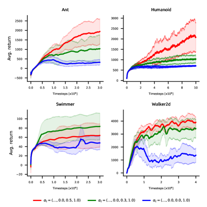
Figure 1: Learning curves with standard deviation error bars for robustness test. We experiment with $\alpha_{t}=(0,0,\ldots,0,\beta,1)$ with $\beta$ in the range of $[0.0,0.3,0.5]$. Setting $\beta$ to values $0.3$ or $0.5$ leads to significantly better robustness to suboptimal hyperparameters than PPO (blue curve).

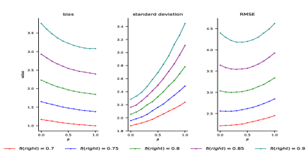
Figure 2: The bias variance trade-off on NChain environment. We investigate $\alpha_{t}=(0,0,\ldots,0,\beta,1)$ for different $\tilde{\pi}(right)\in[0.7,0.75,0.8,0.85,0.9]$. Increasing $\beta$ from $0$ to $1$ reduces the bias but increases the variance of the estimator $L_{\pi}^{\alpha}(\tilde{\pi})$.

Mujoco Environments We follow by carrying out experimentation on high dimensional control problems using Mujoco (Todorov et al., 2012) as a simulator. We adopt the experimental set up from (Schulman et al., 2015a, 2017) and experiment with eight representative Mujoco environments.

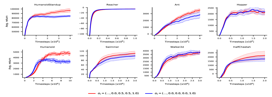
Figure 3: Learning curves for continuous control benchmarks reported with half standard deviation error bars. We compare well-performing choice $\alpha_{t}=(0,0,\ldots,0.0,0.5,0.5,1)$ against PPO (blue curve). The results are averaged over $20$ seeds. Approximate IS Policy Optimization leads to an improved speed of learning on several environments. See text for full details.

In these experiments we use $\alpha_{t}=(0,0,\ldots,0,0.5,0.5,1)$. The benefit of these choice of $\alpha_{t}$ of policy optimization is that it incurs only modest additional computational burden and is straightforward to implement in a practical setting. Note that the choice $\alpha_{t}=(0,0,\ldots,0,0,1)$ corresponds to PPO algorithm. We discuss the results of experimenting with a wide range of different settings of $\alpha_{t}$ later in the text.

We average the learning curves over $20$ random seeds. The results are gathered in Figure 3. We see that Approximate IS Policy Optimization increases speed of learning on five environments: HumanoidStandup, Ant, Swimmer, HalfCheetah and Humanoid and results in the same performance on three environments Walker2d, Hopper and Reacher. We observe a substantial improvement corresponding to $48\%$ increase in sample efficiency on Humanoid environment and average improvement of $20\%$ on four further environments (HumanoidStandup, Ant, Swimmer and HalfCheetah). We report detailed results and all experimental details allowing to replicate the experiments in the Appendix. Note Approximate IS Policy Optimization either outperforms PPO or results in a statistically insignificant difference in returns.

Robustness test Next we test the robustness of Approximate IS Policy Optimization to suboptimal hyperparameters. In practice tuning hyperparameters per environment leads to significant computational burden and often suboptimal hyperparameters have to be used. For this task, we run the algorithm in four Mujoco environments and average the learning curves over $8$ separate seeds. During these experiments we use too high clip value, i.e. $0.4$ for Ant, Swimmer and Walker2d tasks and $0.2$ for Humanoid environment. In this task we again experiment with the choice $\alpha_{t}=(0,0,\ldots,0,\beta,1)$. We report the learning curves in Figure 1. We see that adjusting $\beta$ can dramatically improve sample efficiency of PPO and we observe that the improvement in sample efficiency increases with the value of used $\beta$. While standard PPO is unable to learn on Humanoid task Approximate IS Policy Optimization can provide meaningful policy updates leading to much better performance.

Different schemes of $\alpha_{t}$ We also experiment with choices of $\alpha_{t}=(0,0,\ldots,0,\beta_{3},\beta_{2},\beta_{1})$ and report the results in Table 2. We see that introducing further non-zero components to $\alpha_{t}$ provides improvements when first and second component are added but plateaus for third added component. Investigated choices of $\alpha_{t}$ again provide improvements on five environments out of eight tasks. We also observe that using more complicated schemes of $\alpha_{t}$ than two non-zero components can provide better performance as visible on HumanoidStandup task but generally lead to similar results while requiring additional computation and slightly slowing down the algorithm. We provide extensive comparison of different choices of $\alpha_{t}$ in the Appendix.

7 Conclusions

We introduced a novel approach to policy optimization based on the approximation to importance sampling. We demonstrated that the introduced proxy objective allows to trade-off bias and variance and covers surrogate objective from Schulman et al. (2015a) and importance sampling as special cases. We also derived theoretical results analyzing bias and variance of the introduced objective followed by providing results unifying the previous work on policy improvement. The derived policy optimization procedure led to increase in sample efficiency up to $48\%$ on high dimensional environments such as Humanoid.

Appendix A Appendix

A.1 Skipped proofs

We begin by providing Lemma 6 which we will use to derive proofs of claims present in text.

Lemma 6.

For random variables $\{X_{t}\}_{t=0}^{\infty}$ such that $\exists C>0\ \forall t\geq 0\ |X_{t}|\leq C$ have that

$$\big{(}\sum_{t\geq 0}^{T}\gamma^{t}X_{t}\big{)}^{2}\leq\frac{1-\gamma^{T+1}}{1-\gamma}\sum_{t\geq 0}^{T}\gamma^{t}X_{t}^{2}.$$ (26)

Proof.

By Cauchy-Schwarz inequality we have that:

$$\Big{(}\sum_{t\geq 0}^{T}\gamma^{t}X_{t}\Big{)}^{2}=\Big{(}\sum_{t\geq 0}^{T}\gamma^{t/2}\gamma^{t/2}X_{t}\Big{)}^{2}\leq\sum_{t\geq 0}^{T}\gamma^{t}\sum_{t\geq 0}^{T}\gamma^{t}X_{t}^{2}.$$ (27)

By summing geometric series we obtain

$$\Big{(}\sum_{t\geq 0}^{T}\gamma^{t}X_{t}\Big{)}^{2}\leq\frac{1-\gamma^{T+1}}{1-\gamma}\sum_{t\geq 0}^{T}\gamma^{t}X_{t}^{2}.$$ (28)

∎

Derivation of Lemma 1.

By applying Lemma 6 we have that

$$\Big{(}\sum_{t\geq 0}^{T}\gamma^{t}\rho_{0:t}^{\alpha_{t}}A^{\pi}(s_{t},a_{t})\Big{)}^{2}\leq\frac{1-\gamma^{T+1}}{1-\gamma}\sum_{t\geq 0}^{T}\gamma^{t}(\rho_{0:t}^{\alpha_{t}})^{2}A^{\pi}(s_{t},a_{t})^{2}.$$ (29)

We also have that

$$\sum_{t\geq 0}^{T}\gamma^{t}(\rho_{0:t}^{\alpha_{t}})^{2}A^{\pi}(s_{t},a_{t})^{2}=\sum_{t\geq 0}^{T}\gamma^{t}\prod_{i=0}^{T}(\rho_{i}^{\alpha_{t}^{i}})^{2}A^{\pi}(s_{t},a_{t})^{2}$$ (30)

$$\leq\epsilon^{2}\sum_{t\geq 0}^{T}\gamma^{t}\prod_{i=0}^{T}(\rho_{i}^{\alpha_{t}^{i}})^{2}\leq\epsilon^{2}\sum_{t\geq 0}^{T}\gamma^{t}\prod_{i=0}^{T}C_{\rho}^{2\alpha_{t}^{i}}$$ (31)

$$\leq\epsilon^{2}\sum_{t\geq 0}^{T}\gamma^{t}C_{\rho}^{2\sum_{i=0}^{T}\alpha_{t}^{i}}=\epsilon^{2}\sum_{t\geq 0}^{T}\gamma^{t}C_{\rho}^{2\left\lVert\alpha_{t}\right\rVert_{1}},$$ (32)

where we have used $\epsilon=\max_{s\in\mathcal{S},a\in\mathcal{A}}A^{\pi}(s,a)$ and $\max_{s\in\mathcal{S},a\in\mathcal{A}}\rho(s,a)<C_{\rho}$. We now have

$$\operatorname*{\mathbb{E}}_{\tau\sim\pi}\Big{(}\sum_{t\geq 0}^{T}\gamma^{t}\rho_{0:t}^{\alpha_{t}}A^{\pi}(s_{t},a_{t})\Big{)}^{2}\leq\frac{1-\gamma^{T+1}}{1-\gamma}\operatorname*{\mathbb{E}}_{\tau\sim\pi}\sum_{t\geq 0}^{T}\gamma^{t}(\rho_{0:t}^{\alpha_{t}})^{2}A^{\pi}(s_{t},a_{t})^{2}$$ (33)

$$\leq\epsilon^{2}\operatorname*{\mathbb{E}}_{\tau\sim\pi}\sum_{t\geq 0}^{T}\gamma^{t}C_{\rho}^{2\left\lVert\alpha_{t}\right\rVert_{1}}=\epsilon^{2}\sum_{t\geq 0}^{T}\gamma^{t}C_{\rho}^{2\left\lVert\alpha_{t}\right\rVert_{1}},$$ (34)

and because $\mathbb{V}X=\operatorname*{\mathbb{E}}X^{2}-[\operatorname*{\mathbb{E}}X]^{2}\leq\operatorname*{\mathbb{E}}X^{2}$ we also have

$$\operatorname*{\mathbb{V}}_{\tau\sim\pi}\Big{(}\sum_{t\geq 0}^{T}\gamma^{t}\rho_{0:t}^{\alpha_{t}}A^{\pi}(s_{t},a_{t})\Big{)}^{\leq}\frac{1-\gamma^{T+1}}{1-\gamma}\epsilon^{2}\sum_{t\geq 0}^{T}\gamma^{t}C_{\rho}^{2\left\lVert\alpha_{t}\right\rVert_{1}}.$$ (35)

∎

Derivation of Lemma 2.

We have that

$$\sum_{t\geq 0}^{T}\gamma^{t}\rho_{0:t}^{\alpha_{t}}A^{\pi}(s_{t},a_{t})-\sum_{t\geq 0}^{T}\gamma^{t}\rho_{0:t}A^{\pi}(s_{t},a_{t})=\sum_{t\geq 0}^{T}\gamma^{t}\big{(}\rho_{0:t}^{\alpha_{t}}-\rho_{0:t}\big{)}A^{\pi}(s_{t},a_{t})=\sum_{t\geq 0}^{T}\gamma^{t}\rho_{0:t}\big{(}\rho_{0:t}^{\alpha_{t}}-1\big{)}A^{\pi}(s_{t},a_{t}).$$ (36)

By taking expectation $\operatorname*{\mathbb{E}}_{\tau\sim\pi}$ on both sides we obtain

$$\operatorname*{\mathbb{E}}_{\tau\sim\pi}\sum_{t\geq 0}^{T}\gamma^{t}\rho_{0:t}^{\alpha_{t}}A^{\pi}(s_{t},a_{t})-\sum_{t\geq 0}^{T}\gamma^{t}\rho_{0:t}A^{\pi}(s_{t},a_{t})=\operatorname*{\mathbb{E}}_{\tau\sim\pi}\sum_{t\geq 0}^{T}\gamma^{t}\rho_{0:t}\big{(}\rho_{0:t}^{\alpha_{t}}-1\big{)}A^{\pi}(s_{t},a_{t}).$$ (37)

Next we apply absolute value to both sides which results in

$$\big{|}\operatorname*{\mathbb{E}}_{\tau\sim\pi}\sum_{t\geq 0}^{T}\gamma^{t}\rho_{0:t}^{\alpha_{t}}A^{\pi}(s_{t},a_{t})-\sum_{t\geq 0}^{T}\gamma^{t}\rho_{0:t}A^{\pi}(s_{t},a_{t})\big{|}=\big{|}\operatorname*{\mathbb{E}}_{\tau\sim\pi}\sum_{t\geq 0}^{T}\gamma^{t}\rho_{0:t}\big{(}\rho_{0:t}^{\alpha_{t}}-1\big{)}A^{\pi}(s_{t},a_{t})\big{|}$$ (38)

$$=\big{|}\operatorname*{\mathbb{E}}_{\tau\sim\tilde{\pi}}\sum_{t\geq 0}^{T}\gamma^{t}\big{(}\rho_{0:t}^{\alpha_{t}}-1\big{)}A^{\pi}(s_{t},a_{t})\big{|}\leq\operatorname*{\mathbb{E}}_{\tau\sim\tilde{\pi}}\big{|}\sum_{t\geq 0}^{T}\gamma^{t}\big{(}\rho_{0:t}^{\alpha_{t}}-1\big{)}A^{\pi}(s_{t},a_{t})\big{|}$$ (39)

$$\leq\operatorname*{\mathbb{E}}_{\tau\sim\tilde{\pi}}\sum_{t\geq 0}^{T}\gamma^{t}\big{|}\rho_{0:t}^{\alpha_{t}}-1\big{|}\big{|}A^{\pi}(s_{t},a_{t})\big{|}\leq\operatorname*{\mathbb{E}}_{\tau\sim\tilde{\pi}}\epsilon\sum_{t\geq 0}^{T}\gamma^{t}\big{|}\rho_{0:t}^{\alpha_{t}}-1\big{|}.$$ (40)

where we used $\epsilon=\max_{s\in\mathcal{S},a\in\mathcal{A}}A^{\pi}(s,a)$. ∎

Derivation of Lemma 3.

Recall that based on Equation (4) we have that

$$\nabla\rho_{0:t}^{\alpha_{t}}(s_{0:t},a_{0:t})A^{\pi}(s_{t},a_{t})=\rho_{0:t}^{\alpha_{t}}\sum_{i=0}^{t}\alpha_{t}^{i}\frac{\pi(a_{i}|s_{i})}{\tilde{\pi}(a_{i}|s_{i})}\nabla\tilde{\pi}(a_{i}|s_{i})A^{\pi}(s_{t},a_{t}).$$ (41)

We will use the fact that $\mathrm{tr}\operatorname*{\mathrm{Cov}}[X,X]=\sum_{i=1}^{N}\operatorname*{\mathbb{E}}X_{i}^{2}-[\operatorname*{\mathbb{E}}X_{i}]^{2}\leq\sum_{i=1}^{N}\operatorname*{\mathbb{E}}X_{i}^{2}=\operatorname*{\mathbb{E}}\sum_{i=1}^{N}X_{i}^{2}=\operatorname*{\mathbb{E}}\left\lVert X\right\rVert^{2}_{2}$ to obtain

$$\mathrm{tr}\operatorname*{\mathrm{Cov}}_{\tau\sim\pi}\Big{[}\nabla\sum_{t\geq 0}\gamma^{t}\rho_{0:t}^{\alpha_{t}}(s_{0:t},a_{0:t})A^{\pi}(s_{t},a_{t}),\nabla\sum_{t\geq 0}\gamma^{t}\rho_{0:t}^{\alpha_{t}}(s_{0:t},a_{0:t})A^{\pi}(s_{t},a_{t})\Big{]}$$ (42)

$$\leq\operatorname*{\mathbb{E}}_{\tau\sim\pi}\left\lVert\sum_{t\geq 0}\gamma^{t}\nabla\rho_{0:t}^{\alpha_{t}}(s_{0:t},a_{0:t})A^{\pi}(s_{t},a_{t})\right\rVert^{2}_{2}$$ (43)

$$=\operatorname*{\mathbb{E}}_{\tau\sim\pi}\left\lVert\sum_{t\geq 0}\gamma^{t}\rho_{0:t}^{\alpha_{t}}\sum_{i=0}^{t}\alpha_{t}^{i}\frac{\pi(a_{i}|s_{i})}{\tilde{\pi}(a_{i}|s_{i})}\nabla\tilde{\pi}(a_{i}|s_{i})A^{\pi}(s_{t},a_{t})\right\rVert^{2}_{2}.$$ (44)

Therefore to obtain an upper bound on $\mathrm{tr}\operatorname*{\mathrm{Cov}}_{\tau\sim\pi}\Big{[}\nabla\sum_{t\geq 0}\gamma^{t}\rho_{0:t}^{\alpha_{t}}(s_{0:t},a_{0:t})A^{\pi}(s_{t},a_{t}),\nabla\sum_{t\geq 0}\gamma^{t}\rho_{0:t}^{\alpha_{t}}(s_{0:t},a_{0:t})A^{\pi}(s_{t},a_{t})\Big{]}$ we proceed by upper bounding term $\left\lVert\sum_{t\geq 0}\gamma^{t}\rho_{0:t}^{\alpha_{t}}\sum_{i=0}^{t}\alpha_{t}^{i}\frac{\pi(a_{i}|s_{i})}{\tilde{\pi}(a_{i}|s_{i})}\nabla\tilde{\pi}(a_{i}|s_{i})A^{\pi}(s_{t},a_{t})\right\rVert_{2}$ as follows:

$$\left\lVert\sum_{t\geq 0}\gamma^{t}\rho_{0:t}^{\alpha_{t}}\sum_{i=0}^{t}\alpha_{t}^{i}\frac{\pi(a_{i}|s_{i})}{\tilde{\pi}(a_{i}|s_{i})}\nabla\tilde{\pi}(a_{i}|s_{i})A^{\pi}(s_{t},a_{t})\right\rVert_{2}$$ (45)

$$\leq\sum_{t\geq 0}\left\lVert\gamma^{t}\rho_{0:t}^{\alpha_{t}}\sum_{i=0}^{t}\alpha_{t}^{i}\frac{\pi(a_{i}|s_{i})}{\tilde{\pi}(a_{i}|s_{i})}\nabla\tilde{\pi}(a_{i}|s_{i})A^{\pi}(s_{t},a_{t})\right\rVert_{2}$$ (46)

$$\leq\sum_{t\geq 0}\gamma^{t}\rho_{0:t}^{\alpha_{t}}\sum_{i=0}^{t}\left\lVert\alpha_{t}^{i}\frac{\pi(a_{i}|s_{i})}{\tilde{\pi}(a_{i}|s_{i})}\nabla\tilde{\pi}(a_{i}|s_{i})A^{\pi}(s_{t},a_{t})\right\rVert_{2}$$ (47)

$$\leq\sum_{t\geq 0}\gamma^{t}\rho_{0:t}^{\alpha_{t}}\sum_{i=0}^{t}\alpha_{t}^{i}|A^{\pi}(s_{t},a_{t})|\Big{|}\frac{\pi(a_{i}|s_{i})}{\tilde{\pi}(a_{i}|s_{i})}\Big{|}\left\lVert\nabla\tilde{\pi}(a_{i}|s_{i})\right\rVert_{2}.$$ (48)

We further have that $\left\lVert\nabla\tilde{\pi}(a_{i}|s_{i})\right\rVert_{2}\leq C_{\partial}^{2}$, $|A^{\pi}(s_{t},a_{t})|\leq\epsilon$ and $\big{|}\frac{\tilde{\pi}(a_{i}|s_{i})}{\pi(a_{i}|s_{i})}\big{|}<C_{\delta}$ and $\left\lVert\alpha_{t}\right\rVert_{1}=\sum_{i=0}^{t}\alpha_{t}^{i}$. It follows that

$$\sum_{t\geq 0}\gamma^{t}\rho_{0:t}^{\alpha_{t}}\sum_{i=0}^{t}\alpha_{t}^{i}|A^{\pi}(s_{t},a_{t})|\Big{|}\frac{\pi(a_{i}|s_{i})}{\tilde{\pi}(a_{i}|s_{i})}\Big{|}\left\lVert\nabla\tilde{\pi}(a_{i}|s_{i})\right\rVert^{2}_{2}$$ (49)

$$\leq\epsilon C_{\partial}C_{\delta}\sum_{t\geq 0}\gamma^{t}\rho_{0:t}^{\alpha_{t}}\sum_{i=0}^{t}\alpha_{t}^{i}=\epsilon C_{\partial}C_{\delta}\sum_{t\geq 0}\gamma^{t}\rho_{0:t}^{\alpha_{t}}\left\lVert\alpha_{t}\right\rVert_{1}.$$ (50)

We apply Cauchy-Schwarz inequality to obtain

$$\sum_{t\geq 0}\gamma^{t}\rho_{0:t}^{\alpha_{t}}\left\lVert\alpha_{t}\right\rVert_{1}\leq\sqrt{\sum_{t\geq 0}\gamma^{t}(\rho_{0:t}^{\alpha_{t}})^{2}}\sqrt{\sum_{t\geq 0}\gamma^{t}\left\lVert\alpha_{t}\right\rVert^{2}_{1}}.$$ (51)

So we have

$$\left\lVert\sum_{t\geq 0}\gamma^{t}\rho_{0:t}^{\alpha_{t}}\sum_{i=0}^{t}\alpha_{t}^{i}\frac{\pi(a_{i}|s_{i})}{\tilde{\pi}(a_{i}|s_{i})}\nabla\tilde{\pi}(a_{i}|s_{i})A^{\pi}(s_{t},a_{t})\right\rVert_{2}\leq\epsilon C_{\partial}C_{\delta}\sqrt{\sum_{t\geq 0}\gamma^{t}(\rho_{0:t}^{\alpha_{t}})^{2}}\sqrt{\sum_{t\geq 0}\gamma^{t}\left\lVert\alpha_{t}\right\rVert^{2}_{1}}.$$ (52)

It follows that

$$\left\lVert\sum_{t\geq 0}\gamma^{t}\rho_{0:t}^{\alpha_{t}}\sum_{i=0}^{t}\alpha_{t}^{i}\frac{\pi(a_{i}|s_{i})}{\tilde{\pi}(a_{i}|s_{i})}\nabla\tilde{\pi}(a_{i}|s_{i})A^{\pi}(s_{t},a_{t})\right\rVert_{2}^{2}\leq\epsilon^{2}C_{\partial}^{2}C_{\delta}^{2}\sum_{t\geq 0}\gamma^{t}(\rho_{0:t}^{\alpha_{t}})^{2}\sum_{t\geq 0}\gamma^{t}\left\lVert\alpha_{t}\right\rVert^{2}_{1}.$$ (53)

So we have that

$$\operatorname*{\mathbb{E}}_{\tau\sim\pi}\left\lVert\sum_{t\geq 0}\gamma^{t}\rho_{0:t}^{\alpha_{t}}\sum_{i=0}^{t}\alpha_{t}^{i}\frac{\pi(a_{i}|s_{i})}{\tilde{\pi}(a_{i}|s_{i})}\nabla\tilde{\pi}(a_{i}|s_{i})A^{\pi}(s_{t},a_{t})\right\rVert_{2}^{2}\leq\epsilon^{2}C_{\partial}^{2}C_{\delta}^{2}\sum_{t\geq 0}\gamma^{t}\left\lVert\alpha_{t}\right\rVert^{2}_{1}\operatorname*{\mathbb{E}}_{\tau\sim\pi}\sum_{t\geq 0}\gamma^{t}(\rho_{0:t}^{\alpha_{t}})^{2},$$ (54)

We will now use the assumption hat $\operatorname*{\mathbb{E}}_{\tau\sim\pi}\sum_{t\geq 0}\gamma^{t}(\rho_{0:t}^{\alpha_{t}})^{2}<C^{\gamma}$ so we have that $\sum_{t\geq 0}\gamma^{t}(\rho_{0:t}^{\alpha_{t}})^{2}<C^{\gamma}$. This yields

$$\operatorname*{\mathbb{E}}_{\tau\sim\pi}\left\lVert\sum_{t\geq 0}\gamma^{t}\rho_{0:t}^{\alpha_{t}}\sum_{i=0}^{t}\alpha_{t}^{i}\frac{\pi(a_{i}|s_{i})}{\tilde{\pi}(a_{i}|s_{i})}\nabla\tilde{\pi}(a_{i}|s_{i})A^{\pi}(s_{t},a_{t})\right\rVert_{2}^{2}\leq\epsilon^{2}C_{\partial}^{2}C_{\delta}^{2}C^{\gamma}\sum_{t\geq 0}\gamma^{t}\left\lVert\alpha_{t}\right\rVert^{2}_{1}.$$ (55)

By comparing to inequalities obtained starting from 42 it follows that

$$\mathrm{tr}\operatorname*{\mathrm{Cov}}_{\tau\sim\pi}\Big{[}\nabla\sum_{t\geq 0}\gamma^{t}\rho_{0:t}^{\alpha_{t}}(s_{0:t},a_{0:t})A^{\pi}(s_{t},a_{t}),\nabla\sum_{t\geq 0}\gamma^{t}\rho_{0:t}^{\alpha_{t}}(s_{0:t},a_{0:t})A^{\pi}(s_{t},a_{t})\Big{]}\leq\epsilon^{2}C_{\partial}^{2}C_{\delta}^{2}C^{\gamma}\sum_{t\geq 0}\gamma^{t}\left\lVert\alpha_{t}\right\rVert^{2}_{1},$$ (56)

which concludes the proof. ∎

Derivation of Lemma 4.

We first find an upper bound on $\left\lVert\nabla\sum_{t\geq 0}\rho_{0:t}^{\alpha_{t}}A^{\pi}(s_{t},a_{t})-\nabla\sum_{t\geq 0}\rho_{0:t}A^{\pi}(s_{t},a_{t})\right\rVert_{2}$. We have that

$$\left\lVert\nabla\sum_{t\geq 0}\rho_{0:t}^{\alpha_{t}}A^{\pi}(s_{t},a_{t})-\nabla\sum_{t\geq 0}\rho_{0:t}A^{\pi}(s_{t},a_{t})\right\rVert_{2}$$ (57)

$$=\left\lVert\sum_{t\geq 0}\nabla\rho_{0:t}^{\alpha_{t}}A^{\pi}(s_{t},a_{t})-\nabla\rho_{0:t}A^{\pi}(s_{t},a_{t})\Big{]}\right\rVert_{2}$$ (58)

$$\leq\sum_{t\geq 0}\left\lVert\nabla\rho_{0:t}^{\alpha_{t}}A^{\pi}(s_{t},a_{t})-\nabla\rho_{0:t}A^{\pi}(s_{t},a_{t})\right\rVert_{2}.$$ (59)

By Equation (4) we can express $\nabla\rho_{0:t}^{\alpha_{t}}(s_{0:t},a_{0:t})A^{\pi}(s_{t},a_{t})-\nabla\rho_{0:t}(s_{0:t},a_{0:t})A^{\pi}(s_{t},a_{t})$ as

$$\nabla\rho_{0:t}^{\alpha_{t}}(s_{0:t},a_{0:t})A^{\pi}(s_{t},a_{t})-\nabla\rho_{0:t}(s_{0:t},a_{0:t})A^{\pi}(s_{t},a_{t})$$ (60)

$$=\rho_{0:t}^{\alpha_{t}}\sum_{i=0}^{t}\alpha_{t}^{i}\frac{\pi(a_{i}|s_{i})}{\tilde{\pi}(a_{i}|s_{i})}\nabla\tilde{\pi}(a_{i}|s_{i})A^{\pi}(s_{t},a_{t})-\rho_{0:t}\sum_{i=0}^{t}\frac{\pi(a_{i}|s_{i})}{\tilde{\pi}(a_{i}|s_{i})}\nabla\tilde{\pi}(a_{i}|s_{i})A^{\pi}(s_{t},a_{t})$$ (61)

$$=\sum_{i=0}^{t}\alpha_{t}^{i}\rho_{0:t}^{\alpha_{t}}\frac{\pi(a_{i}|s_{i})}{\tilde{\pi}(a_{i}|s_{i})}\nabla\tilde{\pi}(a_{i}|s_{i})A^{\pi}(s_{t},a_{t})-\sum_{i=0}^{t}\rho_{0:t}\frac{\pi(a_{i}|s_{i})}{\tilde{\pi}(a_{i}|s_{i})}\nabla\tilde{\pi}(a_{i}|s_{i})A^{\pi}(s_{t},a_{t})$$ (62)

$$=\sum_{i=0}^{t}\big{(}\alpha_{t}^{i}\rho_{0:t}^{\alpha_{t}}-\rho_{0:t}\big{)}\frac{\pi(a_{i}|s_{i})}{\tilde{\pi}(a_{i}|s_{i})}\nabla\tilde{\pi}(a_{i}|s_{i})A^{\pi}(s_{t},a_{t}).$$ (63)

So it follows that

$$\left\lVert\nabla\rho_{0:t}^{\alpha_{t}}(s_{0:t},a_{0:t})A^{\pi}(s_{t},a_{t})-\nabla\rho_{0:t}(s_{0:t},a_{0:t})A^{\pi}(s_{t},a_{t})\right\rVert_{2}$$ (64)

$$\left\lVert\sum_{i=0}^{t}\big{(}\alpha_{t}^{i}\rho_{0:t}^{\alpha_{t}}-\rho_{0:t}\big{)}\frac{\pi(a_{i}|s_{i})}{\tilde{\pi}(a_{i}|s_{i})}\nabla\tilde{\pi}(a_{i}|s_{i})A^{\pi}(s_{t},a_{t})\right\rVert_{2}$$ (65)

$$\leq\sum_{i=0}^{t}\left\lVert\big{(}\alpha_{t}^{i}\rho_{0:t}^{\alpha_{t}}-\rho_{0:t}\big{)}\frac{\pi(a_{i}|s_{i})}{\tilde{\pi}(a_{i}|s_{i})}\nabla\tilde{\pi}(a_{i}|s_{i})A^{\pi}(s_{t},a_{t})\right\rVert_{2}$$ (66)

$$=\sum_{i=0}^{t}\big{|}\alpha_{t}^{i}\rho_{0:t}^{\alpha_{t}}-\rho_{0:t}\big{|}\big{|}\frac{\pi(a_{i}|s_{i})}{\tilde{\pi}(a_{i}|s_{i})}\big{|}\big{|}A^{\pi}(s_{t},a_{t})\big{|}\left\lVert\nabla\tilde{\pi}(a_{i}|s_{i})\right\rVert_{2}.$$ (67)

Recall that we have that $\epsilon=\max_{s\in\mathcal{S},a\in\mathcal{A}}|A^{\pi}(s,a)|$ and $\left\lVert\nabla\tilde{\pi}(a_{i}|s_{i})\right\rVert_{2}\leq C^{\partial}$. We proceed by further bounding the term $\sum_{i=0}^{t}\big{|}\alpha_{t}^{i}\rho_{0:t}^{\alpha_{t}}-\rho_{0:t}\big{|}\big{|}\frac{\pi(a_{i}|s_{i})}{\tilde{\pi}(a_{i}|s_{i})}\big{|}\big{|}A^{\pi}(s_{t},a_{t})\big{|}\left\lVert\nabla\tilde{\pi}(a_{i}|s_{i})\right\rVert_{2}$ in the following way:

$$\sum_{i=0}^{t}\big{|}\alpha_{t}^{i}\rho_{0:t}^{\alpha_{t}}-\rho_{0:t}\big{|}\big{|}\frac{\pi(a_{i}|s_{i})}{\tilde{\pi}(a_{i}|s_{i})}\big{|}\big{|}A^{\pi}(s_{t},a_{t})\big{|}\left\lVert\nabla\tilde{\pi}(a_{i}|s_{i})\right\rVert_{2}$$ (68)

$$\leq\epsilon C^{\partial}\sum_{i=0}^{t}\big{|}\alpha_{t}^{i}\rho_{0:t}^{\alpha_{t}}-\rho_{0:t}\big{|}\leq\epsilon C^{\partial}\sum_{i=0}^{t}\big{|}\alpha_{t}^{i}\rho_{0:t}^{\alpha_{t}}-\rho_{0:t}^{\alpha_{t}}+\rho_{0:t}^{\alpha_{t}}-\rho_{0:t}\big{|}$$ (69)

$$\leq\epsilon C^{\partial}\sum_{i=0}^{t}\big{|}(\alpha_{t}^{i}-1)\rho_{0:t}^{\alpha_{t}}|+|\rho_{0:t}^{\alpha_{t}}-\rho_{0:t}\big{|}=\epsilon C^{\partial}\sum_{i=0}^{t}\big{|}(\alpha_{t}^{i}-1)\rho_{0:t}^{\alpha_{t}}|+\sum_{i=0}^{t}|\rho_{0:t}^{\alpha_{t}}-\rho_{0:t}\big{|}$$ (70)

$$=\epsilon C^{\partial}\sum_{i=0}^{t}\big{|}(\alpha_{t}^{i}-1)\rho_{0:t}^{\alpha_{t}}|+(t+1)|\rho_{0:t}^{\alpha_{t}}-\rho_{0:t}\big{|}=\epsilon C^{\partial}\rho_{0:t}^{\alpha_{t}}\sum_{i=0}^{t}\big{|}\alpha_{t}^{i}-1|+\sum_{i=0}^{t}|\rho_{0:t}^{\alpha_{t}}-\rho_{0:t}\big{|}$$ (71)

$$=\epsilon C^{\partial}\sum_{i=0}^{t}\big{|}(\alpha_{t}^{i}-1)\rho_{0:t}^{\alpha_{t}}|+(t+1)|\rho_{0:t}^{\alpha_{t}}-\rho_{0:t}\big{|}=\epsilon C^{\partial}\rho_{0:t}^{\alpha_{t}}\sum_{i=0}^{t}\big{|}\alpha_{t}^{i}-1|+(t+1)|\rho_{0:t}^{\alpha_{t}}-\rho_{0:t}\big{|}$$ (72)

$$=\epsilon C^{\partial}\rho_{0:t}^{\alpha_{t}}\left\lVert\alpha_{t}-\mathbf{1}\right\rVert_{1}+(t+1)|\rho_{0:t}^{\alpha_{t}}-\rho_{0:t}\big{|}.$$ (73)

As a result we have that

$$\left\lVert\nabla\sum_{t\geq 0}\gamma^{t}\rho_{0:t}^{\alpha_{t}}A^{\pi}(s_{t},a_{t})-\nabla\sum_{t\geq 0}\gamma^{t}\rho_{0:t}A^{\pi}(s_{t},a_{t})\right\rVert_{2}\leq\epsilon C^{\partial}\sum_{t\geq 0}\gamma^{t}\Big{[}\rho_{0:t}^{\alpha_{t}}\left\lVert\alpha_{t}-\mathbf{1}\right\rVert_{1}+(t+1)|\rho_{0:t}^{\alpha_{t}}-\rho_{0:t}\big{|}\Big{]}.$$ (74)

∎

Derivation of Lemma 5.

The equality in Equation (2) is symmetrical w.r.t. policies $\pi$ and $\tilde{\pi}$. We can write

$$\eta(\pi)-\eta(\tilde{\pi})=\frac{1}{1-\gamma}\mathbb{E}_{s\sim d^{\pi},a\sim\pi(\cdot|s)}A^{\tilde{\pi}}(s,a).$$ (75)

It follows that

$$\eta(\pi)-\eta(\tilde{\pi})=\frac{1}{1-\gamma}\mathbb{E}_{s\sim d^{\pi},a\sim\pi(\cdot|s)}A^{\tilde{\pi}}(s,a)=$$ (76)

$$=\frac{1}{1-\gamma}\mathbb{E}_{s\sim d^{\pi}}\Big{[}\int\tilde{\pi}(a|s)A^{\pi}(s,a)da-\int\tilde{\pi}(a|s)A^{\pi}(s,a)da+\int\pi(a|s)A^{\tilde{\pi}}(s,a)da\Big{]}$$ (77)

$$=-L_{\pi}(\tilde{\pi})+\frac{1}{1-\gamma}\mathbb{E}_{s\sim d^{\pi}}\Big{[}\int\tilde{\pi}(a|s)A^{\pi}(s,a)da+\int\pi(a|s)A^{\tilde{\pi}}(s,a)da\Big{]}$$ (78)

$$=-L_{\pi}(\tilde{\pi})+\frac{1}{1-\gamma}\mathbb{E}_{s\sim d^{\pi}}\Big{[}\int\tilde{\pi}(a|s)Q^{\pi}(s,a)da+\int\pi(a|s)Q^{\tilde{\pi}}(s,a)da-V^{\tilde{\pi}}(s)-V^{\pi}(s)\Big{]}$$ (79)

$$=-L_{\pi}(\tilde{\pi})+\frac{1}{1-\gamma}\mathbb{E}_{s\sim d^{\pi}}\Big{[}\int\tilde{\pi}(a|s)Q^{\pi}(s,a)da+\int\pi(a|s)Q^{\tilde{\pi}}(s,a)da$$

$$-\int\tilde{\pi}(a|s)Q^{\tilde{\pi}}(s,a)da-\int\pi(a|s)Q^{\pi}(s,a)da\Big{]}$$ (80)

$$=-L_{\pi}(\tilde{\pi})+\frac{1}{1-\gamma}\mathbb{E}_{s\sim d^{\pi}}\Big{[}\int\tilde{\pi}(a|s)\big{(}Q^{\pi}(s,a)-Q^{\tilde{\pi}}(s,a)\big{)}da+\int\pi(a|s)\big{(}Q^{\tilde{\pi}}(s,a)-Q^{\pi}(s,a)\big{)}da\Big{]}$$ (81)

$$=-L_{\pi}(\tilde{\pi})+\frac{1}{1-\gamma}\mathbb{E}_{s\sim d^{\pi}}\Big{[}\int\tilde{\pi}(a|s)\big{(}Q^{\pi}(s,a)-Q^{\tilde{\pi}}(s,a)\big{)}da-\int\pi(a|s)\big{(}Q^{\pi}(s,a)-Q^{\tilde{\pi}}(s,a)\big{)}da\Big{]}$$ (82)

$$=-L_{\pi}(\tilde{\pi})+\frac{1}{1-\gamma}\mathbb{E}_{s\sim d^{\pi}}\Big{[}\int\big{(}\tilde{\pi}(a|s)-\pi(a|s)\big{)}\big{(}Q^{\pi}(s,a)-Q^{\tilde{\pi}}(s,a)\big{)}da\Big{]}$$ (83)

$$=-L_{\pi}(\tilde{\pi})-\frac{1}{1-\gamma}\mathbb{E}_{s\sim d^{\pi}}\Big{[}\int\big{(}\tilde{\pi}(a|s)-\pi(a|s)\big{)}\big{(}Q^{\tilde{\pi}}(s,a)-Q^{\pi}(s,a)\big{)}da\Big{]}.$$ (84)

So we obtain that

$$\eta(\pi)-\eta(\tilde{\pi})=-L_{\pi}(\tilde{\pi})-\frac{1}{1-\gamma}\mathbb{E}_{s\sim d^{\pi}}\int\big{(}\tilde{\pi}(a|s)-\pi(a|s)\big{)}\big{(}Q^{\tilde{\pi}}(s,a)-Q^{\pi}(s,a)\big{)}da.$$ (85)

After multiplying by $-1$ this gives

$$\eta(\tilde{\pi})-\eta(\pi)=L_{\pi}(\tilde{\pi})+\frac{1}{1-\gamma}\mathbb{E}_{s\sim d^{\pi}}\int\big{(}\tilde{\pi}(a|s)-\pi(a|s)\big{)}\big{(}Q^{\tilde{\pi}}(s,a)-Q^{\pi}(s,a)\big{)}da.$$ (86)

∎

Note that the integral $\int\big{(}\tilde{\pi}(a|s)-\pi(a|s)\big{)}\big{(}Q^{\tilde{\pi}}(s,a)-Q^{\pi}(s,a)\big{)}da$ can be viewed as a weighted total variation distance between $\pi$ and $\tilde{\pi}$ where weights are defined by $Q^{\tilde{\pi}}(s,a)-Q^{\pi}(s,a)$. It follows that the divergence of policies $\pi$ and $\tilde{\pi}$ on state-action pairs $(s,a)$ having large difference in value $Q^{\tilde{\pi}}(s,a)-Q^{\pi}(s,a)$ is causing degradation in the performance of approximation of $L_{\pi}(\tilde{\pi})$. Also $Q^{\tilde{\pi}}(s,a)-Q^{\pi}(s,a)$ can be viewed as weighting current difference between policies $\pi$ and $\tilde{\pi}$ by delayed effect of the difference arising from $Q^{\tilde{\pi}}(s,a)-Q^{\pi}(s,a)$.

A.2 Derivations of the results from literature

We first provide the following Corollary which we will use to derive Policy Gradient Theorems. The result follows from the following algebraic transformations applied to Equation (5).

Corollary 7 (Value dependency equality).

Given two policies $\tilde{\pi}$ and $\pi$,

$$\eta(\tilde{\pi})-\eta(\pi)=\frac{1}{1-\gamma}\operatorname*{\mathbb{E}}_{s\sim d^{\pi}}\int\big{(}\tilde{\pi}(a|s)-\pi(a|s)\big{)}Q^{\tilde{\pi}}(s,a)da.$$ (87)

Proof.

$$\eta(\tilde{\pi})=\eta(\pi)+L_{\pi}(\tilde{\pi})+\frac{1}{1-\gamma}\operatorname*{\mathbb{E}}_{s\sim d^{\pi}}\int\big{(}Q^{\tilde{\pi}}(s,a)-Q^{\pi}(s,a)\big{)}\big{(}\tilde{\pi}(a|s)-\pi(a|s)\big{)}da$$ (88)

$$=\eta(\pi)+\frac{1}{1-\gamma}\operatorname*{\mathbb{E}}_{s\sim d^{\pi}}\int\tilde{\pi}(a|s)A^{\pi}(s,a)da+\frac{1}{1-\gamma}\operatorname*{\mathbb{E}}_{s\sim d^{\pi}}\int\big{(}Q^{\tilde{\pi}}(s,a)-Q^{\pi}(s,a)\big{)}\big{(}\tilde{\pi}(a|s)-\pi(a|s)\big{)}da$$ (89)

$$=\eta(\pi)+\frac{1}{1-\gamma}\operatorname*{\mathbb{E}}_{s\sim d^{\pi}}\Big{[}\int\tilde{\pi}(a|s)Q^{\pi}(s,a)da-V^{\pi}(s)\Big{]}+\frac{1}{1-\gamma}\operatorname*{\mathbb{E}}_{s\sim d^{\pi}}\int\big{(}Q^{\tilde{\pi}}(s,a)-Q^{\pi}(s,a)\big{)}\big{(}\tilde{\pi}(a|s)-\pi(a|s)\big{)}da$$ (90)

$$=\eta(\pi)+\frac{1}{1-\gamma}\operatorname*{\mathbb{E}}_{s\sim d^{\pi}}\Big{[}\int\tilde{\pi}(a|s)Q^{\pi}(s,a)da-\int\pi(a|s)Q^{\pi}(s,a)da\Big{]}+$$

$$+\frac{1}{1-\gamma}\operatorname*{\mathbb{E}}_{s\sim d^{\pi}}\int\Big{[}\tilde{\pi}(a|s)Q^{\tilde{\pi}}(s,a)-\tilde{\pi}(a|s)Q^{\pi}(s,a)-\pi(a|s)Q^{\tilde{\pi}}(s,a)+\pi(a|s)Q^{\pi}(s,a)\Big{]}da$$ (91)

$$=\eta(\pi)+\frac{1}{1-\gamma}\operatorname*{\mathbb{E}}_{s\sim d^{\pi}}\int\tilde{\pi}(a|s)Q^{\tilde{\pi}}(s,a)-\pi(a|s)Q^{\tilde{\pi}}(s,a)da$$ (92)

$$=\eta(\pi)+\frac{1}{1-\gamma}\operatorname*{\mathbb{E}}_{s\sim d^{\pi}}\int\big{(}\tilde{\pi}(a|s)-\pi(a|s)\big{)}Q^{\tilde{\pi}}(s,a)da.$$ (93)

∎

Alternative derivation of Corollary 7.

Again, by using symmetry in Equation (2) we obtain:

$$\eta(\pi)-\eta(\tilde{\pi})=+\frac{1}{1-\gamma}\mathbb{E}_{s\sim d^{\pi}}\int\pi(a|s)A^{\tilde{\pi}}(s,a)da.$$ (94)

It follows that

$$\eta(\tilde{\pi})=\eta(\pi)-\frac{1}{1-\gamma}\mathbb{E}_{s\sim d^{\pi}}\int\pi(a|s)A^{\tilde{\pi}}(s,a)da$$ (95)

$$\eta(\tilde{\pi})=\eta(\pi)-\frac{1}{1-\gamma}\mathbb{E}_{s\sim d^{\pi}}\Big{[}-\int\tilde{\pi}(a|s)A^{\tilde{\pi}}(s,a)da+\int\pi(a|s)A^{\tilde{\pi}}(s,a)da\Big{]}$$ (96)

$$\eta(\tilde{\pi})=\eta(\pi)-\frac{1}{1-\gamma}\mathbb{E}_{s\sim d^{\pi}}\Big{[}\int\tilde{\pi}(a|s)\Big{(}V^{\tilde{\pi}}(s)-Q^{\tilde{\pi}}(s,a)\Big{)}da+\int\pi(a|s)\Big{(}Q^{\tilde{\pi}}(s,a)-V^{\tilde{\pi}}(s)\Big{)}da\Big{]}$$ (97)

$$\eta(\tilde{\pi})=\eta(\pi)-\frac{1}{1-\gamma}\mathbb{E}_{s\sim d^{\pi}}\Big{[}-\int\tilde{\pi}(a|s)Q^{\tilde{\pi}}(s,a)da+V^{\tilde{\pi}}(s)+\int\pi(a|s)Q^{\tilde{\pi}}(s,a)da-V^{\tilde{\pi}}(s)\Big{]}$$ (98)

$$\eta(\tilde{\pi})=\eta(\pi)-\frac{1}{1-\gamma}\mathbb{E}_{s\sim d^{\pi}}\Big{[}-\int\tilde{\pi}(a|s)Q^{\tilde{\pi}}(s,a)da+\int\pi(a|s)Q^{\tilde{\pi}}(s,a)da\Big{]}$$ (99)

$$\eta(\tilde{\pi})=\eta(\pi)+\frac{1}{1-\gamma}\mathbb{E}_{s\sim d^{\pi}}\int\big{(}\tilde{\pi}(a|s)-\pi(a|s)\big{)}Q^{\tilde{\pi}}(s,a)da.$$ (100)

∎

We begin by providing short derivations of theorems obtained in previous works of Sutton et al. (1999); Silver et al. (2014); Ciosek & Whiteson (2018). To simplify notation, for parametrized policies, we denote target policy $\tilde{\pi}$ as $\pi_{\theta}$ and behavior policy $\pi$ as $\pi_{\theta_{0}}$.

Equation (87) requires access to state-action value function $Q^{\pi_{\theta}}$ of the target policy. Nevertheless, we show that Corollary 7 can be used to unify and easily derive previously proven policy gradient theorems (Sutton et al., 1999; Silver et al., 2014; Ciosek & Whiteson, 2018). These results follow from the fact that the state occupancy measure on the RHS does not depend on target policy $\pi_{\theta}$, so the RHS can be easily differentiated with respect to its parameters.

Derivation of Policy Gradient Theorem (Theorem 1) from (Sutton et al., 1999).

We differentiate expression for $\eta(\pi_{\theta})$ from Corollary 7:

$$\frac{\partial}{\partial\theta}\eta(\pi_{\theta})=\frac{\partial}{\partial\theta}\Bigg{[}\eta(\pi_{\theta_{0}})+\frac{1}{1-\gamma}\operatorname*{\mathbb{E}}_{s\sim d^{\pi}}\int Q^{\pi_{\theta}}(s,a)\big{(}\pi_{\theta}(a|s)-\pi_{\theta_{0}}(a|s)\big{)}da\Bigg{]}=$$ (101)

$$=\frac{1}{1-\gamma}\Bigg{[}\operatorname*{\mathbb{E}}_{s\sim d^{\pi}}\int\frac{\partial}{\partial\theta}Q^{\pi_{\theta}}(s,a)\big{(}\pi_{\theta}(a|s)-\pi_{\theta_{0}}(a|s)\big{)}da+\int Q^{\pi_{\theta}}(s,a)\frac{\partial}{\partial\theta}\big{(}\pi_{\theta}(a|s)-\pi_{\theta_{0}}(a|s)\big{)}da\Bigg{]}$$ (102)

$$=\frac{1}{1-\gamma}\Bigg{[}\operatorname*{\mathbb{E}}_{s\sim d^{\pi}}\int\frac{\partial}{\partial\theta}Q^{\pi_{\theta}}(s,a)\big{(}\pi_{\theta}(a|s)-\pi_{\theta_{0}}(a|s)\big{)}da+\int Q^{\pi_{\theta}}(s,a)\frac{\partial}{\partial\theta}\pi_{\theta}(a|s)da\Bigg{]}.$$ (103)

By evaluating derivative at $\theta=\theta_{0}$ we obtain:

$$\frac{\partial}{\partial\theta}\eta(\pi_{\theta})\Big{|}_{\theta=\theta_{0}}=\frac{1}{1-\gamma}\operatorname*{\mathbb{E}}_{s\sim d^{\pi}}\int\frac{\partial}{\partial\theta}\pi_{\theta}(a|s)\Big{|}_{\theta=\theta_{0}}Q^{\pi_{\theta_{0}}}(s,a)da.$$ (104)

After applying $\frac{\partial}{\partial x}f(x)=f(x)\frac{\partial}{\partial x}\log f(x)$:

$$\frac{\partial}{\partial\theta}\eta(\pi_{\theta})\Big{|}_{\theta=\theta_{0}}=\frac{1}{1-\gamma}\operatorname*{\mathbb{E}}_{s\sim d^{\pi}}\int\pi_{\theta_{0}}(a|s)\frac{\partial}{\partial\theta}\log\pi_{\theta}(a|s)\Big{|}_{\theta=\theta_{0}}Q^{\pi_{\theta_{0}}}(s,a)da.$$ (105)

∎

Derivation of Deterministic Policy Gradient Theorem (Theorem 1 from Silver et al. (2014)).

Again, we differentiate the expression for $\eta(\pi_{\theta})$ from Corollary 7

$$\frac{\partial}{\partial\theta}\eta(\pi_{\theta})=\frac{\partial}{\partial\theta}\Bigg{[}\eta(\pi_{\theta_{0}})+\frac{1}{1-\gamma}\operatorname*{\mathbb{E}}_{s\sim d^{\pi}}Q^{\pi_{\theta}}(s,\pi_{\theta}(s))-Q^{\pi_{\theta}}(s,\pi_{\theta_{0}}(s))\Bigg{]}=$$ (106)

$$=\frac{1}{1-\gamma}\Bigg{[}\operatorname*{\mathbb{E}}_{s\sim d^{\pi}}\frac{\partial}{\partial\theta}Q^{\pi_{\theta}}(s,\pi_{\theta}(s))-\frac{\partial}{\partial\theta}Q^{\pi_{\theta}}(s,\pi_{\theta_{0}}(s))\Bigg{]}$$ (107)

$$=\frac{1}{1-\gamma}\Bigg{[}\operatorname*{\mathbb{E}}_{s\sim d^{\pi}}\frac{\partial}{\partial a}Q^{\pi_{\theta}}(s,a)\frac{\partial}{\partial\theta}\pi_{\theta}(s)+\frac{\partial}{\partial\theta}Q^{\pi_{\theta}}(s,\pi_{\theta}(s))-\frac{\partial}{\partial\theta}Q^{\pi_{\theta}}(s,\pi_{\theta_{0}}(s))\Bigg{]}.$$ (108)

Where we calculate total derivative = $\frac{\partial}{\partial\theta}Q^{\pi_{\theta}}(s,\pi_{\theta}(s))=\frac{\partial}{\partial\pi_{\theta}(s)}Q^{\pi_{\theta}}(s,\pi_{\theta}(s))+\frac{\partial}{\partial\theta}Q^{\pi_{\theta}}(s,\pi_{\theta}(s))$ and then use chain rule to get $\frac{\partial}{\partial\pi_{\theta}(s)}Q^{\pi_{\theta}}(s,\pi_{\theta}(s))=\frac{\partial}{\partial a}Q^{\pi_{\theta}}(s,a)|_{a=\pi_{\theta}(s)}\frac{\partial}{\partial\theta}\pi_{\theta}(s)$. By evaluating derivative at $\theta=\theta_{0}$ we obtain:

$$\frac{\partial}{\partial\theta}\eta(\pi_{\theta})\Big{|}_{\theta=\theta_{0}}=\frac{1}{1-\gamma}\operatorname*{\mathbb{E}}_{s\sim d^{\pi}}\frac{\partial}{\partial a}Q^{\pi_{\theta_{0}}}(s,a)\Big{|}_{a=\pi_{\theta_{0}}(s)}\frac{\partial}{\partial\theta}\pi_{\theta}(s)\Big{|}_{\theta=\theta_{0}}.$$ (109)

∎

Derivation of General Policy Gradient Theorem (Theorem 1 from Ciosek & Whiteson (2018)).

This result also follows from differentiating expression for $\eta(\pi_{\theta})$ from Corollary 7

$$\frac{\partial}{\partial\theta}\eta(\pi_{\theta})=\frac{\partial}{\partial\theta}\Bigg{[}\eta(\pi_{\theta_{0}})+\frac{1}{1-\gamma}\operatorname*{\mathbb{E}}_{s\sim d^{\pi}}\int Q^{\pi_{\theta}}(s,a)\big{(}\pi_{\theta}(a|s)-\pi_{\theta_{0}}(a|s)\big{)}da\Bigg{]}$$ (110)

$$=\frac{\partial}{\partial\theta}\frac{1}{1-\gamma}\operatorname*{\mathbb{E}}_{s\sim d^{\pi}}\Bigg{[}\int Q^{\pi_{\theta}}(s,a)\pi_{\theta}(a|s)da-\int\pi_{\theta_{0}}(a|s)Q^{\pi_{\theta}}(s,a)da\Bigg{]}=$$ (111)

$$=\frac{\partial}{\partial\theta}\frac{1}{1-\gamma}\operatorname*{\mathbb{E}}_{s\sim d^{\pi}}\Bigg{[}V^{\pi_{\theta}}(s)-\int\pi_{\theta_{0}}(a|s)Q^{\pi_{\theta}}(s,a)da\Bigg{]}$$ (112)

$$=\frac{1}{1-\gamma}\operatorname*{\mathbb{E}}_{s\sim d^{\pi}}\Bigg{[}\frac{\partial}{\partial\theta}V^{\pi_{\theta}}(s)-\int\pi_{\theta_{0}}(a|s)\frac{\partial}{\partial\theta}Q^{\pi_{\theta}}(s,a)da\Bigg{]}.$$ (113)

By evaluating derivative at $\theta=\theta_{0}$ we derive

$$\frac{\partial}{\partial\theta}\eta(\pi_{\theta})\Big{|}_{\theta=\theta_{0}}=\frac{1}{1-\gamma}\operatorname*{\mathbb{E}}_{s\sim d^{\pi}}\Bigg{[}\frac{\partial}{\partial\theta}V^{\pi_{\theta}}(s)\Big{|}_{\theta=\theta_{0}}-\int\pi_{\theta_{0}}(a|s)\frac{\partial}{\partial\theta}Q^{\pi_{\theta}}(s,a)\Big{|}_{\theta=\theta_{0}}da\Bigg{]}.$$ (114)

∎

Next, we derive the previously obtained bounds on the quality of approximation of $L_{\pi}(\tilde{\pi})$. We firstly prove a lemma used in these derivations.

Lemma 8.

Given two policies $\tilde{\pi}$ and $\pi$, the following equality holds

$$\operatorname*{\mathbb{E}}_{\tau\sim\tilde{\pi}|s,a}\sum_{t\geq 1}\gamma^{t-1}A^{\pi}(s_{t},a_{t})=\frac{1}{\gamma}\big{(}Q^{\tilde{\pi}}(s,a)-Q^{\pi}(s,a)\big{)}.$$ (115)

Proof.

We apply the following algebraic transformations

$$\operatorname*{\mathbb{E}}_{\tau\sim\tilde{\pi}}[\sum_{t\geq 1}\gamma^{t-1}A^{\pi}(s_{t},a_{t})|s_{0}=s,a_{0}=a]=\sum_{t\geq 1}\operatorname*{\mathbb{E}}_{s_{t},s_{t+1}}[\gamma^{t-1}\big{(}r(s_{t},a_{t})+\gamma V^{\pi}(s_{t+1})-V^{\pi}(s_{t})\big{)}|s_{0}=s,a_{0}=a]$$ (116)

$$=\operatorname*{\mathbb{E}}_{\tau\sim\tilde{\pi}}[-V^{\pi}(s_{1})+\sum_{t\geq 1}\gamma^{t-1}r(s_{t},a_{t})|s_{0}=s,a_{0}=a]=\operatorname*{\mathbb{E}}_{p(s^{\prime}|s,a)}-V^{\pi}(s^{\prime})+V^{\tilde{\pi}}(s^{\prime})=\operatorname*{\mathbb{E}}_{p(s^{\prime}|s,a)}V^{\tilde{\pi}}(s^{\prime})-V^{\pi}(s^{\prime})$$ (117)

$$=\frac{1}{\gamma}\operatorname*{\mathbb{E}}_{p(s^{\prime}|s,a)}\gamma V^{\tilde{\pi}}(s^{\prime})-\gamma V^{\pi}(s^{\prime})=\frac{1}{\gamma}\operatorname*{\mathbb{E}}_{p(s^{\prime}|s,a)}\gamma V^{\tilde{\pi}}(s^{\prime})+r(s,a)-\gamma V^{\pi}(s^{\prime})-r(s,a)=\frac{1}{\gamma}\big{(}Q^{\tilde{\pi}}(s,a)-Q^{\pi}(s,a)\big{)}.$$ (118)

∎

Derivation of Corollary 1 from from Achiam et al. (2017).

Note that when $\epsilon=\max_{s}|\operatorname*{\mathbb{E}}_{a\sim\tilde{\pi}(\cdot|s)}A^{\pi}(s,a)|$ we have that $\frac{\epsilon}{1-\gamma}\geq\operatorname*{\mathbb{E}}_{\tau\sim\tilde{\pi}|s,a}\sum_{t\geq 1}\gamma^{t-1}|\operatorname*{\mathbb{E}}_{a\sim\tilde{\pi}(\cdot|s_{t})}A^{\pi}(s_{t},a)|$. From Lemma 8 we have that $Q^{\tilde{\pi}}(s,a)-Q^{\pi}(s,a)=\gamma\operatorname*{\mathbb{E}}_{\tau\sim\tilde{\pi}|s,a}\sum_{t\geq 1}\gamma^{t-1}A^{\pi}(s_{t},a_{t})$. It follows that

$$\Big{|}\eta(\tilde{\pi})-\eta(\pi)-L_{\tilde{\pi}}(\pi)\Big{|}=$$ (119)

$$=\frac{1}{1-\gamma}\Big{|}\operatorname*{\mathbb{E}}_{s\sim d^{\pi}}\int\big{(}Q^{\tilde{\pi}}(s,a)-Q^{\pi}(s,a)\big{)}\big{(}\tilde{\pi}(a|s)-\pi(a|s)\big{)}\Big{|}da$$ (120)

$$=\frac{1}{1-\gamma}\Big{|}\operatorname*{\mathbb{E}}_{s\sim d^{\pi}}\int\gamma\Big{[}\operatorname*{\mathbb{E}}_{\tau\sim\tilde{\pi}|s,a}\sum_{t\geq 1}\gamma^{t-1}A^{\pi}(s_{t},a_{t})\Big{]}\big{(}\tilde{\pi}(a|s)-\pi(a|s)\big{)}\Big{|}da$$ (121)

$$\leq\frac{1}{1-\gamma}\operatorname*{\mathbb{E}}_{s\sim d^{\pi}}\int\frac{\gamma\epsilon}{1-\gamma}\Big{|}\tilde{\pi}(a|s)-\pi(a|s)\Big{|}da$$ (122)

$$=\frac{2\epsilon\gamma}{(1-\gamma)^{2}}\operatorname*{\mathbb{E}}_{s\sim d^{\pi}}\frac{1}{2}\int\Big{|}\tilde{\pi}(a|s)-\pi(a|s)\Big{|}da$$ (123)

$$=\frac{2\epsilon\gamma}{(1-\gamma)^{2}}\operatorname*{\mathbb{E}}_{s\sim d^{\pi}}\mathbb{D}_{\mathcal{TV}}\big{(}\tilde{\pi}(\cdot|s)||\pi(\cdot|s)\big{)}.$$ (124)

∎

Derivation of Theorem 1 from Schulman et al. (2015a).

Let $\epsilon=\max_{s,a}|A^{\pi}(s,a)|$. We note that $\gamma|\operatorname*{\mathbb{E}}_{\tau\sim\tilde{\pi}|s,a}\sum_{t\geq 1}\gamma^{t-1}A^{\pi}(s_{t},a_{t})|\leq\frac{2\epsilon\gamma}{1-\gamma}\max_{s}\mathbb{D}_{\mathcal{TV}}\big{(}\tilde{\pi}(\cdot|s)||\pi(\cdot|s)\big{)}$. It follows from: for any $s$ the expected advantage $\int\pi(a|s)A^{\pi}(s,a)da=0$, so we have $|\operatorname*{\mathbb{E}}_{\tau\sim\tilde{\pi}|s,a}\sum_{t\geq 1}\gamma^{t-1}A^{\pi}(s_{t},a_{t})|=|\operatorname*{\mathbb{E}}_{\tau\sim\tilde{\pi}|s,a}\sum_{t\geq 1}\gamma^{t-1}\big{(}\tilde{\pi}(a_{t}|s_{t})-\pi(a_{t}|s_{t})\big{)}A^{\pi}(s_{t},a_{t})|\leq\operatorname*{\mathbb{E}}_{\tau\sim\tilde{\pi}|s,a}\sum_{t\geq 1}\gamma^{t-1}|\tilde{\pi}(a_{t}|s_{t})-\pi(a_{t}|s_{t})||A^{\pi}(s_{t},a_{t})|\leq\frac{2\epsilon}{1-\gamma}\max_{s}D^{TV}(\tilde{\pi}(\cdot|s)||\pi(\cdot|s))$ . We follow by

$$\Big{|}\eta(\tilde{\pi})-\eta(\pi)-L_{\tilde{\pi}}(\pi)\Big{|}=$$ (125)

$$=\frac{1}{1-\gamma}\Big{|}\operatorname*{\mathbb{E}}_{s\sim d^{\pi}(s)}\int\big{(}Q^{\tilde{\pi}}(s,a)-Q^{\pi}(s,a)\big{)}\big{(}\tilde{\pi}(a|s)-\pi(a|s)\big{)}\Big{|}da$$ (126)

$$=\frac{1}{1-\gamma}\Big{|}\operatorname*{\mathbb{E}}_{s\sim d^{\pi}(s)}\int\gamma\Big{[}\operatorname*{\mathbb{E}}_{\tau\sim\tilde{\pi}|s,a}\sum_{t\geq 1}\gamma^{t-1}A_{\pi}(s_{t},a_{t})\Big{]}\big{(}\tilde{\pi}(a|s)-\pi(a|s)\big{)}\Big{|}da$$ (127)

$$=\frac{1}{1-\gamma}\Big{|}\operatorname*{\mathbb{E}}_{s\sim d^{\pi}(s)}\frac{2\epsilon\gamma}{1-\gamma}\max_{s}\mathbb{D}_{\mathcal{TV}}\big{(}\tilde{\pi}(\cdot|s)||\pi(\cdot||s)\big{)}\big{(}\tilde{\pi}(a|s)-\pi(a|s)\big{)}\Big{|}$$ (128)

$$\leq\frac{4\epsilon\gamma}{(1-\gamma)^{2}}\max_{s}\mathbb{D}_{\mathcal{TV}}\big{(}\tilde{\pi}(\cdot|s)||\pi(\cdot||s)\big{)}^{2}.$$ (129)

∎

Derivation of first inequality from Theorem 2 from Gu et al. (2017).

We introduce the following notation target policy $\tilde{\pi}$, policy gathering the current batch of data $\pi$ and policy providing off-policy data $\beta$. Denote vector $f^{\pi,\tilde{\pi}}$ as a vector with components $f^{\pi,\tilde{\pi}}(s)=\operatorname*{\mathbb{E}}_{a\sim\tilde{\pi}(\cdot|s)}A^{\pi}(s,a)$. Also, denote $f_{w}^{\pi,\tilde{\pi}}$ parametric approximation to $f^{\pi,\tilde{\pi}}$ with coordinates $f^{\pi,\tilde{\pi}}(s)=\operatorname*{\mathbb{E}}_{a\sim\tilde{\pi}(\cdot|s)}A^{\pi}_{w}(s,a)$. By using Lemma 5:

$$(1-\gamma)\big{(}\eta(\tilde{\pi})-\eta(\pi)\big{)}=\langle d^{\pi},f^{\pi,\tilde{\pi}}\rangle+\operatorname*{\mathbb{E}}_{s\sim d^{\pi}}\int\big{(}Q^{\tilde{\pi}}(s,a)-Q^{\pi}(s,a)\big{)}\big{(}\tilde{\pi}(a|s)-\pi(a|s)\big{)}da.$$ (130)

We can use the following representation for $\langle d^{\pi},f^{\pi,\tilde{\pi}}\rangle$:

$$\langle d^{\pi},f^{\pi,\tilde{\pi}}\rangle=(1-\alpha)\langle d^{\pi},f^{\pi,\tilde{\pi}}\rangle+\alpha\langle d^{\pi},f^{\pi,\tilde{\pi}}-f_{w}^{\pi,\tilde{\pi}}\rangle+\alpha\langle d^{\beta},f_{w}^{\pi,\tilde{\pi}}\rangle+\alpha\langle d^{\pi}-d^{\beta},f_{w}^{\pi,\tilde{\pi}}\rangle.$$ (131)

Following (Gu et al., 2017) define $\tilde{L}_{\pi,\beta}(\tilde{\pi}):=(1-\alpha)\frac{1}{1-\gamma}\operatorname*{\mathbb{E}}_{s\sim d^{\pi},a\sim\tilde{\pi}(\cdot|s)}A^{\pi}(s,a)+\alpha\frac{1}{1-\gamma}\operatorname*{\mathbb{E}}_{s\sim d^{\beta},a\sim\tilde{\pi}(\cdot|s)}A_{w}^{\pi}(s,a)$ and we denote $\delta:=\max_{s,a}|A^{\pi}(s,a)-\tilde{A}_{w}^{\pi}(s,a)|$, $\zeta:=\max_{s}|f^{\pi,\tilde{\pi}}(s)|$ and $\epsilon:=\max_{s}|f_{w}^{\pi,\tilde{\pi}}(s)|$. We then have that

$$(1-\gamma)\big{(}\eta(\tilde{\pi})-\eta(\pi)\big{)}-\tilde{L}_{\pi,\beta}(\tilde{\pi})\big{)}=\alpha\langle d^{\pi},f^{\pi,\tilde{\pi}}-f_{w}^{\pi,\tilde{\pi}}\rangle+\alpha\langle d^{\pi}-d^{\beta},f_{w}^{\pi,\tilde{\pi}}\rangle$$

$$+\operatorname*{\mathbb{E}}_{s\sim d^{\pi}}\int\big{(}Q^{\tilde{\pi}}(s,a)-Q^{\pi}(s,a)\big{)}\big{(}\tilde{\pi}(a|s)-\pi(a|s)\big{)}da.$$ (132)

and

$$\eta(\tilde{\pi})-\eta(\pi)-\tilde{L}_{\pi,\beta}(\tilde{\pi})=\frac{1}{1-\gamma}\Big{[}\alpha\langle d^{\pi},f_{w}^{\pi,\tilde{\pi}}-f^{\pi,\tilde{\pi}}\rangle+\alpha\langle d^{\pi}-d^{\beta},f^{\pi,\tilde{\pi}}\rangle$$

$$+\operatorname*{\mathbb{E}}_{s\sim d^{\pi}}\int\big{(}Q^{\tilde{\pi}}(s,a)-Q^{\pi}(s,a)\big{)}\big{(}\tilde{\pi}(a|s)-\pi(a|s)\big{)}da\Big{]}.$$ (133)

We now bound separate terms: $|\langle d^{\pi},f_{w}^{\pi,\tilde{\pi}}-f^{\pi,\tilde{\pi}}\rangle|\leq\delta$ and $|\operatorname*{\mathbb{E}}_{s\sim d^{\pi}}\int(Q^{\tilde{\pi}}(s,a)-Q^{\pi}(s,a)\big{)}\big{(}\tilde{\pi}(a|s)-\pi(a|s)\big{)}da|\leq\zeta\operatorname*{\mathbb{E}}_{s\sim d^{\pi}}\int|\tilde{\pi}(a|s)-\pi(a|s)\big{|}da$. By applying Holder inequality to $\langle d^{\pi}-d^{\beta},f^{\pi,\tilde{\pi}}\rangle$ we obtain $|\langle d^{\pi}-d^{\beta},f^{\pi,\tilde{\pi}}\rangle|\leq||d^{\pi}-d^{\beta}||_{1}||f^{\pi,\tilde{\pi}}||_{\infty}$. By using Lemma 3 from Appendix in Achiam et al. (2017) we get $||d^{\pi}-d^{\beta}||_{1}\leq\frac{2\gamma}{1-\gamma}\operatorname*{\mathbb{E}}_{s\sim d^{\pi}}D^{TV}(\pi(\cdot|s)||\beta(\cdot|s))$. As a result $|\langle d^{\pi}-d^{\beta},f^{\pi,\tilde{\pi}}\rangle|\leq\frac{2\gamma\zeta}{1-\gamma}\operatorname*{\mathbb{E}}_{s\sim d^{\pi}}D^{TV}(\pi(\cdot|s)||\beta(\cdot|s))$. Combining these inequalities yields:

$$\Big{|}\eta(\tilde{\pi})-\eta(\pi)-\tilde{L}_{\pi,\beta}(\tilde{\pi})\Big{|}\leq\frac{1}{1-\gamma}\Big{[}\alpha\delta+\frac{2\alpha\epsilon\gamma}{1-\gamma}\operatorname*{\mathbb{E}}_{s\sim d^{\pi}}D^{TV}(\tilde{\pi}(\cdot|s)||\pi(\cdot|s))+\frac{2\gamma\zeta}{1-\gamma}\operatorname*{\mathbb{E}}_{s\sim d^{\pi}}D^{TV}(\pi(\cdot|s)||\beta(\cdot|s))\Big{]}.$$ (134)

We can then use the inequality $\operatorname*{\mathbb{E}}_{s\sim d^{\pi}}D^{TV}(\pi(\cdot|s)||\tilde{\pi}(\cdot|s))\leq\sqrt{\frac{1}{2}\operatorname*{\mathbb{E}}_{s\sim d^{\pi}}D^{KL}(\pi(\cdot|s)||\tilde{\pi}(\cdot|s))}$ to obtain

$$\Big{|}\eta(\tilde{\pi})-\eta(\pi)-\tilde{L}_{\pi,\beta}(\tilde{\pi})\Big{|}\leq\frac{1}{1-\gamma}\Big{[}\alpha\delta+\frac{1}{\sqrt{2}}\frac{2\alpha\epsilon\gamma}{1-\gamma}\sqrt{\operatorname*{\mathbb{E}}_{s\sim d^{\pi_{1}}}D^{KL}(\tilde{\pi}(\cdot|s)||\pi(\cdot|s))}+\frac{2\gamma\zeta}{\sqrt{2}}\frac{1}{1-\gamma}\sqrt{\operatorname*{\mathbb{E}}_{s\sim d^{\pi_{1}}}D^{KL}(\pi(\cdot|s)||,\pi_{2}(\cdot|s))}\Big{]}.$$ (135)

Using $\operatorname*{\mathbb{E}}_{s\sim d^{\beta}}D^{KL}(\pi(\cdot|s)||\tilde{\pi}(\cdot|s))\leq\max_{s}D^{KL}(\pi(\cdot|s)||\tilde{\pi}(\cdot|s))$ for any policy $\beta$ and upper bounding $\frac{1}{\sqrt{2}}<1$ we obtain the bound from Gu et al. (2017):

$$\Big{|}\eta(\tilde{\pi})-\eta(\pi)-\tilde{L}_{\pi,\beta}(\tilde{\pi})\Big{|}\leq\frac{1}{1-\gamma}\Big{[}\alpha\delta+\frac{2\alpha\epsilon\gamma}{1-\gamma}\sqrt{\max_{s}D^{KL}(\tilde{\pi}(\cdot|s)||\pi(\cdot|s))}+\frac{2\gamma\zeta}{1-\gamma}\sqrt{\max_{s}D^{KL}(\pi(\cdot|s)||\beta(\cdot|s))}\Big{]}.$$

∎

Derivation of second inequality from Theorem 2 from Gu et al. (2017).

To prove equality two from Theorem 2 we define $\tilde{L}_{\pi,\beta}^{CV}(\tilde{\pi}):=(1-\alpha)\frac{1}{1-\gamma}\operatorname*{\mathbb{E}}_{s\sim d^{\pi},a\sim\tilde{\pi}(\cdot|s)}(A^{\pi}(s,a)-A^{\pi}_{w}(s,a))+\frac{1}{1-\gamma}\operatorname*{\mathbb{E}}_{s\sim d^{\beta},a\sim\tilde{\pi}(\cdot|s)}A_{w}^{\pi}(s,a)$. We can use the following representation for $\langle d^{\pi},f^{\pi,\tilde{\pi}}\rangle$:

$$\langle d^{\pi},f^{\pi,\tilde{\pi}}\rangle=(1-\alpha)\langle d^{\pi},f^{\pi,\tilde{\pi}}-f_{w}^{\pi,\tilde{\pi}}\rangle+\langle d^{\beta},f_{w}^{\pi,\tilde{\pi}}\rangle+\alpha\langle d^{\pi},f^{\pi,\tilde{\pi}}-f_{w}^{\pi,\tilde{\pi}}\rangle+\langle d^{\pi}-d^{\beta},f_{w}^{\pi,\tilde{\pi}}\rangle.$$ (136)

We can bound separate terms as follows: $|\langle d^{\pi},f^{\pi,\tilde{\pi}}-f_{w}^{\pi,\tilde{\pi}}\rangle|\leq\delta$, we use again $|\langle d^{\pi}-d^{\beta},f^{\pi,\tilde{\pi}}\rangle|\leq\frac{2\gamma\zeta}{1-\gamma}\operatorname*{\mathbb{E}}_{s\sim d^{\pi}}D^{TV}(\pi(\cdot|s)||\beta(\cdot|s))$. By applying Lemma 5 it follows that:

$$\eta(\tilde{\pi})-\eta(\pi)-\tilde{L}^{CV}_{\pi,\beta}(\tilde{\pi})=\frac{1}{1-\gamma}\Big{[}\alpha\langle d^{\pi},f^{\pi,\tilde{\pi}}-f_{w}^{\pi,\tilde{\pi}}\rangle+\langle d^{\pi}-d^{\beta},f_{w}^{\pi,\tilde{\pi}}\rangle+\operatorname*{\mathbb{E}}_{s\sim d^{\pi}}\int\big{(}Q^{\tilde{\pi}}(s,a)-Q^{\pi}(s,a)\big{)}\big{(}\tilde{\pi}(a|s)-\pi(a|s)\big{)}da\Big{]}.$$ (137)

As previously we can use $|\operatorname*{\mathbb{E}}_{s\sim d^{\pi}}\int(Q^{\tilde{\pi}}(s,a)-Q^{\pi}(s,a)\big{)}\big{(}\tilde{\pi}(a|s)-\pi(a|s)\big{)}da|\leq\frac{2\gamma\zeta}{1-\gamma}\sqrt{\max_{s}D^{KL}(\tilde{\pi}(\cdot|s)||\pi(\cdot|s))}$ and $|\langle d^{\pi}-d^{\beta},f_{w}^{\pi,\tilde{\pi}}\rangle|\leq\frac{2\epsilon\gamma}{1-\gamma}\sqrt{\max_{s}D^{KL}(\tilde{\pi}(\cdot|s)||\beta(\cdot|s))}$ to obtain:

$$\Big{|}\eta(\tilde{\pi})-\eta(\pi)-\tilde{L}^{CV}_{\pi,\beta}(\tilde{\pi})\Big{|}\leq\frac{1}{1-\gamma}\Big{[}\alpha\delta+\frac{2\epsilon\gamma}{1-\gamma}\sqrt{\max_{s}D^{KL}(\tilde{\pi}(\cdot|s)||\pi(\cdot|s))}+\frac{2\gamma\zeta}{1-\gamma}\sqrt{\max_{s}D^{KL}(\pi(\cdot|s)||\beta(\cdot|s))}\Big{]}.$$ (138)

∎

A.3 Experimental setup

To ensure meaningful comparison, we alter only the PPO policy optimization objective, switching accordingly to Table 1 and keeping any other hyperparameters or parts of the experimental setup unchanged. To parametrize the policy, we use two layer hidden network with tanh activations outputing the mean of Gaussian distribution over actions. The policy standard deviation is parametrized, but state independent. We use two hidden layer neural network for the value function which we learn by minimising the square loss of predicted values with empirical returns. We use $2048$ transitions to perform the policy update.

To optimize policies we use ADAM optimizer (Kingma & Ba, 2014) with learning rate set to $3\cdot 10^{-4}$ and $\epsilon=10^{-5}$, keeping other default Adam parameters. For every policy update we perform $320$ minibatch optimization steps with the minibatch size of $64$. We use the clip range of $0.2$. For GAE critic, we use standard values of discount $\gamma=0.99$ and lambda factor $\lambda=0.95$. We decay the clip range and learning rate linearly with the passed time steps from the initial values to zeros. We do not use entropy exploration bonus in the course of experiments. We do not perform any environment specific tuning of hyperparameters; we keep hyperparameters fixed during the experimentation. We use only one actor to gather the data required for the policy update. For Humanoid Mujoco experiment we use slightly lower clip value of $0.1$ and constant learning rate schedule. We normalize the state by the moving average of mean and standard deviation.

While performing experiments on Mujoco environments we use standard PPO parameters as listed above. Using environment specific parameters allows to obtain better results, however in this experiment we are aiming to test the robustness of the algorithm.

We report the moving average return over last $200$ episodes as a function of interactions with simulator. We average learning curves over $10$ seeds for Mujoco Humanoid, $20$ seeds for other Mujoco environments and $8$ seeds for Roboschool Humanoid. We based our implementation on publicly available OpenAI Baselines code (Dhariwal et al., 2017). We open source the code used to run the experiments: https://github.com/marctom/POTAIS.

A.4 Further experimental results

We report comparison of the learning curves for additional settings of $\alpha_{t}$ and numerical values obtained during experimentation. As discussed setting $\alpha_{t}\neq(0,\ldots,0,1)$ provides visible improvements on several environments. Introducing further non-zero components provides gains in results for first and second component but not for third introduced component.

$\alpha_{t}$	Standup	Ant	Hopper	Humanoid	Swimmer	Walker2d	HalfCheetah
1.0, 1.0, 1.0	$97751.61\pm 3035.67$	$3240.09\pm 178.5$	$2306.52\pm 202.03$	$4593.64\pm 174.61$	$109.85\pm 6.94$	$3492.56\pm 274.9$	$1747.97\pm 414.25$
0.0, 1.0, 1.0	$97620.58\pm 2632.96$	$3482.96\pm 271.26$	$2241.08\pm 176.55$	$4744.86\pm 96.31$	$107.67\pm 9.02$	$3648.88\pm 246.6$	$1869.14\pm 428.66$
0.0, 0.0, 1.0	$84469.91\pm 1715.18$	$2833.46\pm 445.97$	$2171.21\pm 242.25$	$3241.8\pm 226.38$	$98.94\pm 11.83$	$3814.08\pm 245.67$	$1764.34\pm 310.65$
0.0, 0.0, 0.5	$75367.84\pm 2344.67$	$569.62\pm 122.73$	$2205.87\pm 246.24$	$1709.43\pm 262.64$	$103.85\pm 10.69$	$2527.38\pm 479.23$	$2446.52\pm 602.89$
0.0, 0.5, 1.0	$89588.09\pm 1885.68$	$3268.42\pm 347.93$	$2188.41\pm 215.1$	$4427.96\pm 288.42$	$113.23\pm 6.56$	$3850.1\pm 224.68$	$2044.55\pm 484.02$
0.5, 0.5, 1.0	$96514.29\pm 3524.44$	$3529.4\pm 192.12$	$2112.9\pm 214.03$	$4741.39\pm 235.57$	$110.29\pm 9.41$	$3728.18\pm 218.05$	$2175.29\pm 510.66$
0.5, 0.5, 0.5	$100208.41\pm 4092.96$	$3204.55\pm 208.36$	$2281.64\pm 199.03$	$4618.06\pm 165.57$	$105.0\pm 6.96$	$3639.47\pm 276.92$	$2184.15\pm 481.82$
0.0, 0.0, 0.25	$73079.89\pm 2007.63$	$46.07\pm 23.06$	$1375.32\pm 348.86$	$745.95\pm 36.9$	$91.84\pm 16.29$	$566.21\pm 116.52$	$2688.29\pm 533.54$
0.25, 0.5, 1.0	$93785.21\pm 2962.43$	$3340.99\pm 385.43$	$2111.29\pm 214.28$	$4657.25\pm 176.76$	$113.9\pm 6.66$	$3824.08\pm 246.22$	$1604.46\pm 261.9$
0.25, 0.25, 0.25	$89172.19\pm 2127.32$	$3396.38\pm 121.09$	$2220.28\pm 201.53$	$3741.41\pm 141.29$	$108.15\pm 3.44$	$3423.39\pm 217.89$	$2477.07\pm 551.84$
0.5, 0.5, 0.5, 1.0	$100912.25\pm 3823.57$	$3509.53\pm 161.82$	$2124.92\pm 135.99$	$4810.98\pm 200.86$	$113.66\pm 5.76$	$3871.68\pm 187.82$	$1820.97\pm 416.67$

Table 3: Mean scores obtained for Mujoco experiments with standard deviation error bars averaged over $20$ seeds.

$\alpha_{t}$	$\frac{\eta(\pi_{AISPO})}{\eta(\pi_{PPO})}$
$(0,\ldots,0.0,0.0,0.25)$	$0.73\pm 0.12$
$(0,\ldots,0.0,0.0,0.0,0.5)$	$0.87\pm 0.12$
$(0,\ldots,0.0,0.0,0.0,1.0)$	$1.0\pm 0.1$
$(0,\ldots,0.0,0.0,0.5,1.0)$	$1.1\pm 0.1$
$(0,\ldots,0.0,0.0,1.0,1.0)$	$1.13\pm 0.09$
$(0,\ldots,0.0,0.5,0.5,1.0)$	$\bf{1.14\pm 0.1}$
$(0,\ldots,0.0,0.5,0.5,0.5)$	$\bf{1.14\pm 0.1}$
$(0,\ldots,0.0,0.25,0.5,1.0)$	$1.1\pm 0.09$
$(0,\ldots,0.0,0.25,0.25,0.25)$	$1.11\pm 0.09$
$(0,\ldots,0.0,1.0,1.0,1.0)$	$1.11\pm 0.09$
$(0,\ldots,0.0,0.5,0.5,0.5,1.0)$	$1.13\pm 0.08$

Table 4: Mean relative improvement over PPO for different choices of $\alpha_{t}$ with standard deviation error bars averaged over $20$ seeds.

We present learning curves for different choices of $\alpha_{t}$.

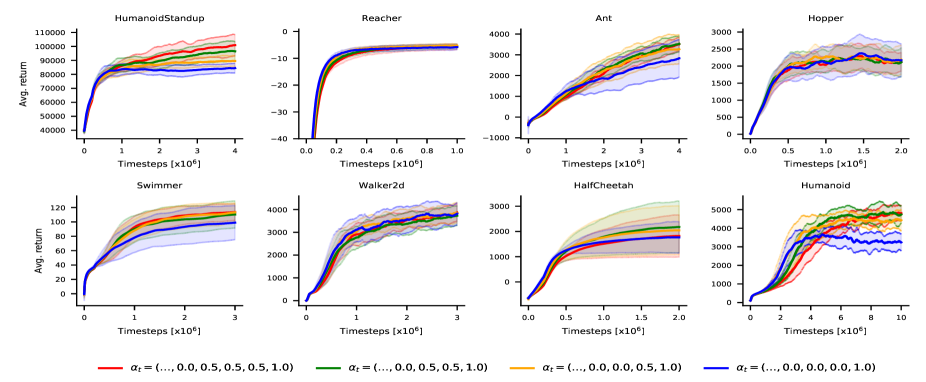
Figure 4: The effect of adding non-zero components $\beta$ when $\alpha_{t}=(0,\ldots,0.0,\beta,\ldots,\beta,1)$. Adding first and second non-zero component provides visible improvements in performance but adding third component does not improve mean performance across environments. Blue curve corresponds to PPO.

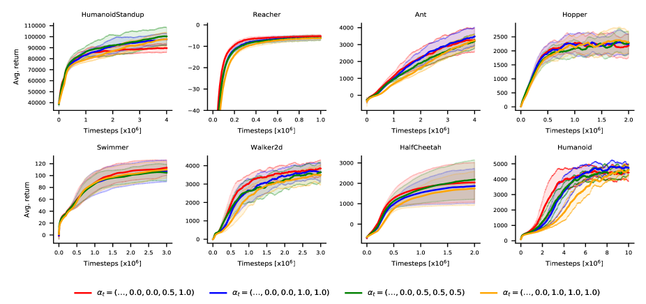
Figure 5: The effect of changing values of components $\beta_{1}$, $\beta_{2}$ and $\beta_{3}$ when $\alpha_{t}=(0,\ldots,0,\beta_{1},\beta_{2},\beta_{3})$. All choices improve over PPO.

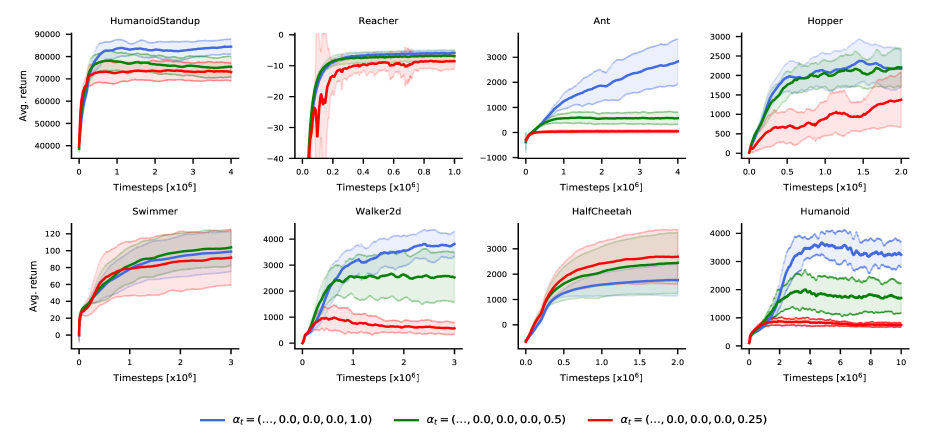
Figure 6: Comparison of $\alpha_{t}=(0,\ldots,0.0,\beta)$. Smoothing the last component reduces the variance but provides excessive bias. This degrades the performance on most environments. Interestingly the performance on HalfCheetah environment improves.

References

- Achiam et al. (2017) Achiam, J., Held, D., Tamar, A., and Abbeel, P. Constrained policy optimization. In Precup, D. and Teh, Y. W. (eds.), Proceedings of the 34th International Conference on Machine Learning, volume 70 of Proceedings of Machine Learning Research, pp. 22–31, International Convention Centre, Sydney, Australia, 06–11 Aug 2017. PMLR. URL http://proceedings.mlr.press/v70/achiam17a.html.
- Ciosek & Whiteson (2018) Ciosek, K. and Whiteson, S. Expected policy gradients. In Thirty-Second AAAI Conference on Artificial Intelligence, 2018.
- Dhariwal et al. (2017) Dhariwal, P., Hesse, C., Klimov, O., Nichol, A., Plappert, M., Radford, A., Schulman, J., Sidor, S., Wu, Y., and Zhokhov, P. Openai baselines, 2017.
- Duan et al. (2016) Duan, Y., Chen, X., Houthooft, R., Schulman, J., and Abbeel, P. Benchmarking deep reinforcement learning for continuous control. In Proceedings of the 33rd International Conference on International Conference on Machine Learning - Volume 48, ICML’16, pp. 1329–1338. JMLR.org, 2016. URL http://dl.acm.org/citation.cfm?id=3045390.3045531.
- Espeholt et al. (2018) Espeholt, L., Soyer, H., Munos, R., Simonyan, K., Mnih, V., Ward, T., Doron, Y., Firoiu, V., Harley, T., Dunning, I., Legg, S., and Kavukcuoglu, K. IMPALA: Scalable distributed deep-RL with importance weighted actor-learner architectures. In Dy, J. and Krause, A. (eds.), Proceedings of the 35th International Conference on Machine Learning, volume 80 of Proceedings of Machine Learning Research, pp. 1407–1416, Stockholmsmässan, Stockholm Sweden, 10–15 Jul 2018. PMLR. URL http://proceedings.mlr.press/v80/espeholt18a.html.
- Fujimoto et al. (2018) Fujimoto, S., van Hoof, H., and Meger, D. Addressing function approximation error in actor-critic methods. In Dy, J. G. and Krause, A. (eds.), Proceedings of the 35th International Conference on Machine Learning, ICML 2018, Stockholmsmässan, Stockholm, Sweden, July 10-15, 2018, volume 80 of Proceedings of Machine Learning Research, pp. 1582–1591. PMLR, 2018. URL http://proceedings.mlr.press/v80/fujimoto18a.html.
- Gu et al. (2017) Gu, S. S., Lillicrap, T., Turner, R. E., Ghahramani, Z., Schölkopf, B., and Levine, S. Interpolated policy gradient: Merging on-policy and off-policy gradient estimation for deep reinforcement learning. In Guyon, I., Luxburg, U. V., Bengio, S., Wallach, H., Fergus, R., Vishwanathan, S., and Garnett, R. (eds.), Advances in Neural Information Processing Systems 30, pp. 3846–3855. Curran Associates, Inc., 2017.
- Jiang & Li (2016) Jiang, N. and Li, L. Doubly robust off-policy value evaluation for reinforcement learning. In Balcan, M. F. and Weinberger, K. Q. (eds.), Proceedings of The 33rd International Conference on Machine Learning, volume 48 of Proceedings of Machine Learning Research, pp. 652–661, New York, New York, USA, 20–22 Jun 2016. PMLR. URL http://proceedings.mlr.press/v48/jiang16.html.
- Kakade & Langford (2002) Kakade, S. and Langford, J. Approximately optimal approximate reinforcement learning. In Proceedings of the Nineteenth International Conference on Machine Learning, ICML ’02, pp. 267–274, San Francisco, CA, USA, 2002. Morgan Kaufmann Publishers Inc. ISBN 1-55860-873-7. URL http://dl.acm.org/citation.cfm?id=645531.656005.
- Kingma & Ba (2014) Kingma, D. P. and Ba, J. Adam: A method for stochastic optimization. arXiv preprint arXiv:1412.6980, 2014.
- Kirkpatrick et al. (1983) Kirkpatrick, S., Gelatt, C. D., and Vecchi, M. P. Optimization by simulated annealing. Science, 220(4598):671–680, 1983. ISSN 0036-8075. doi: 10.1126/science.220.4598.671. URL https://science.sciencemag.org/content/220/4598/671.
- Lillicrap et al. (2015) Lillicrap, T. P., Hunt, J. J., Pritzel, A., Heess, N., Erez, T., Tassa, Y., Silver, D., and Wierstra, D. Continuous control with deep reinforcement learning. arXiv preprint arXiv:1509.02971, 2015.
- Mahmood & Sutton (2015) Mahmood, A. R. and Sutton, R. Off-policy learning based on weighted importance sampling with linear computational complexity. 07 2015.
- Metelli et al. (2018) Metelli, A. M., Papini, M., Faccio, F., and Restelli, M. Policy optimization via importance sampling. In Bengio, S., Wallach, H., Larochelle, H., Grauman, K., Cesa-Bianchi, N., and Garnett, R. (eds.), Advances in Neural Information Processing Systems 31, pp. 5442–5454. Curran Associates, Inc., 2018.
- Mnih et al. (2013) Mnih, V., Kavukcuoglu, K., Silver, D., Graves, A., Antonoglou, I., Wierstra, D., and Riedmiller, M. Playing atari with deep reinforcement learning, 2013.
- Munos et al. (2016) Munos, R., Stepleton, T., Harutyunyan, A., and Bellemare, M. Safe and efficient off-policy reinforcement learning. In Lee, D. D., Sugiyama, M., Luxburg, U. V., Guyon, I., and Garnett, R. (eds.), Advances in Neural Information Processing Systems 29, pp. 1054–1062. Curran Associates, Inc., 2016.
- Pirotta et al. (2013) Pirotta, M., Restelli, M., Pecorino, A., and Calandriello, D. Safe policy iteration. In Dasgupta, S. and McAllester, D. (eds.), Proceedings of the 30th International Conference on Machine Learning, volume 28 of Proceedings of Machine Learning Research, pp. 307–315, Atlanta, Georgia, USA, 17–19 Jun 2013. PMLR. URL http://proceedings.mlr.press/v28/pirotta13.html.
- Precup et al. (2000) Precup, D., Sutton, R. S., and Singh, S. Eligibility traces for off-policy policy evaluation. In Proceedings of the Seventeenth International Conference on Machine Learning, pp. 759–766. Morgan Kaufmann, 2000.
- Schulman et al. (2015a) Schulman, J., Levine, S., Abbeel, P., Jordan, M., and Moritz, P. Trust region policy optimization. In Bach, F. and Blei, D. (eds.), Proceedings of the 32nd International Conference on Machine Learning, volume 37 of Proceedings of Machine Learning Research, pp. 1889–1897, Lille, France, 07–09 Jul 2015a. PMLR. URL http://proceedings.mlr.press/v37/schulman15.html.
- Schulman et al. (2015b) Schulman, J., Moritz, P., Levine, S., Jordan, M., and Abbeel, P. High-dimensional continuous control using generalized advantage estimation. arXiv preprint arXiv:1506.02438, 2015b.
- Schulman et al. (2017) Schulman, J., Wolski, F., Dhariwal, P., Radford, A., and Klimov, O. Proximal policy optimization algorithms. CoRR, abs/1707.06347, 2017. URL http://arxiv.org/abs/1707.06347.
- Silver et al. (2014) Silver, D., Lever, G., Heess, N., Degris, T., Wierstra, D., and Riedmiller, M. Deterministic policy gradient algorithms. In Xing, E. P. and Jebara, T. (eds.), Proceedings of the 31st International Conference on Machine Learning, volume 32 of Proceedings of Machine Learning Research, pp. 387–395, Bejing, China, 22–24 Jun 2014. PMLR. URL http://proceedings.mlr.press/v32/silver14.html.
- Strens (2000) Strens, M. J. A. A bayesian framework for reinforcement learning. In Proceedings of the Seventeenth International Conference on Machine Learning, ICML ’00, pp. 943–950, San Francisco, CA, USA, 2000. Morgan Kaufmann Publishers Inc. ISBN 1-55860-707-2. URL http://dl.acm.org/citation.cfm?id=645529.658114.
- Sutton & Barto (1998) Sutton, R. S. and Barto, A. G. Introduction to Reinforcement Learning. MIT Press, Cambridge, MA, USA, 1st edition, 1998. ISBN 0262193981.
- Sutton et al. (1999) Sutton, R. S., McAllester, D., Singh, S., and Mansour, Y. Policy gradient methods for reinforcement learning with function approximation. In Proceedings of the 12th International Conference on Neural Information Processing Systems, NIPS’99, pp. 1057–1063, Cambridge, MA, USA, 1999. MIT Press. URL http://dl.acm.org/citation.cfm?id=3009657.3009806.
- Thomas & Brunskill (2016) Thomas, P. and Brunskill, E. Data-efficient off-policy policy evaluation for reinforcement learning. In Balcan, M. F. and Weinberger, K. Q. (eds.), Proceedings of The 33rd International Conference on Machine Learning, volume 48 of Proceedings of Machine Learning Research, pp. 2139–2148, New York, New York, USA, 20–22 Jun 2016. PMLR. URL http://proceedings.mlr.press/v48/thomasa16.html.
- Thomas et al. (2015a) Thomas, P., Theocharous, G., and Ghavamzadeh, M. High confidence policy improvement. In Bach, F. and Blei, D. (eds.), Proceedings of the 32nd International Conference on Machine Learning, volume 37 of Proceedings of Machine Learning Research, pp. 2380–2388, Lille, France, 07–09 Jul 2015a. PMLR. URL http://proceedings.mlr.press/v37/thomas15.html.
- Thomas et al. (2015b) Thomas, P. S., Theocharous, G., and Ghavamzadeh, M. High confidence off-policy evaluation. In Proceedings of the Twenty-Ninth AAAI Conference on Artificial Intelligence, AAAI’15, pp. 3000–3006. AAAI Press, 2015b. ISBN 0-262-51129-0. URL http://dl.acm.org/citation.cfm?id=2888116.2888134.
- Todorov et al. (2012) Todorov, E., Erez, T., and Tassa, Y. Mujoco: A physics engine for model-based control. pp. 5026–5033, 10 2012. ISBN 978-1-4673-1737-5. doi: 10.1109/IROS.2012.6386109.
- Tomczak et al. (2019) Tomczak, M. B., Macua, S. V., de Cote, E. M., and Vrancx, P. Compatible features for monotonic policy improvement. In NeurIPS 2019 Optimization Foundations of Reinforcement Learning Workshop, 12 2019. URL https://optrl2019.github.io/assets/accepted_papers/71.pdf.
- van Hasselt et al. (2018) van Hasselt, H., Doron, Y., Strub, F., Hessel, M., Sonnerat, N., and Modayil, J. Deep reinforcement learning and the deadly triad. ArXiv, abs/1812.02648, 2018.