Disruption of Supernovae and would-be “Direct Collapsars”

Abstract

The speed of an intensity pattern of polarization currents on a circle, induced within a star by its rotating, magnetized core, will exceed the speed of light for a sufficiently large star, and/or rapid rotation, and will, in turn, generate focused electromagnetic beams which disrupt them. Upon core collapse within such a star, the emergence of these beams will concentrate near the two rotational poles, driving jets of matter into material previously ejected via the same excitation mechanism acting through the pre-core-collapse rotation of its magnetized stellar core(s). This interpenetration of material, light-days in extent from the progenitor, produces a significant fraction of the total supernova luminosity, and the magnitude and time of maximum of this contribution both vary with the progenitor’s rotational orientation. The net effect is to render supernovae unusable as standard candles without further detailed understanding, leaving no firm basis, at this time, to favor any cosmology, including those involving “Dark Energy.” Thus we are not now, nor have we ever been, in an era of precision cosmology, nor are we likely to be anytime soon. Mass loss induced through the same mechanism also keeps aggregates of gas and plasma in the early Universe, or at any other epoch, from forming the $\sim$billion solar mass stars which have been suggested to produce $\sim$billion solar mass black holes via “direct collapse,” but can also provide a signature to predict core collapse some months in advance. We examine this mechanism through pulsar emission via polarization currents, in which the emission power from any coaxial annulus of plasma decays only as 1/distance for two exactly opposite rotational latitudes given by $\pm\arccos(\mathrm{c}/v)$, where c is the speed of light, and $v>\mathrm{c}$ is the speed of the rotating excitation. We investigate why this effect results from circularly supraluminal excitations, as well as providing a discussion of, and further evidence for, the effect in the Parkes Multibeam Pulsar Survey.

I Introduction

An obliquely magnetized neutron star with an angular velocity of $\omega$ radians/s, will excite polarization currents in the surrounding plasma at projected radius, $R$, with a circumferential pattern, which, for $\omega R>\mathrm{c}$, exceeds the speed of light. The modelAr94 ; H98 ; AR03 ; AR04 ; AR07 ; AR08 ; AR08a of pulsar emission, which takes such supraluminally excited polarization currents into account, is the only model thus far to predict the observed emission bands and their increasing spacing with radio frequencyHE07 in the GHz spectrum of the Crab pulsar interpulse, in addition to matching its observed spectrum out to the $\gamma$-ray — over 15 orders of magnitude (see also [9]).

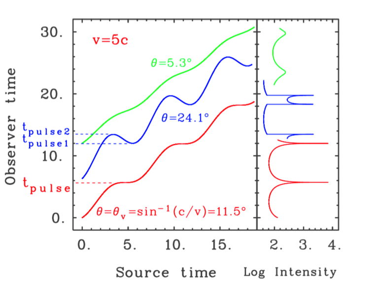
Figure 1: From [M12, ]. Left: Observer time as a function of Source time for a supraluminally induced circular excitation at 5 times light speed, with a frequency of $\omega=1$ radians/s, or a period of $2\pi/\omega=2\pi$ seconds, at a radius $R=5\mathrm{c}/\omega$, where c is the speed of light, for three spin co-latitudes, $\theta$ (polar angles). The three curves have been arbitrarily offset by a few units for clarity. The difference between times for an observer on the distant ($+Y,Z$) plane and the source on the R-circle (centered at the origin, $(X,Y)=(0,0)$) can be expressed as: $t_{\mathrm{obs}}=t_{\mathrm{src}}-R/\mathrm{c}~{}\sin(\omega t_{\mathrm{src}})\sin(\theta)$. Its derivative with respect to time is given by: $\partial t_{\mathrm{obs}}/\partial t_{\mathrm{src}}=1-(\omega R/\mathrm{c})~{}\cos(\omega t_{\mathrm{src}})\sin(\theta)$. The second derivative, $\partial^{2}t_{\mathrm{obs}}/\partial^{2}t_{\mathrm{src}}=(\omega^{2}R/\mathrm{c})~{}\sin(\omega t_{\mathrm{src}})\sin{\theta}$, is zero twice every period, and every other zero is a point of inflection, provided $\theta=\arcsin(\mathrm{c}/(\omega R))$, making the first derivative 0. The other zeros mark the times of maximum slope. Right: the integral, for 65,536 Source times per cycle, into 512 discrete bins per cycle of Observer time/phase, for the three curves (i.e., pulse profiles).

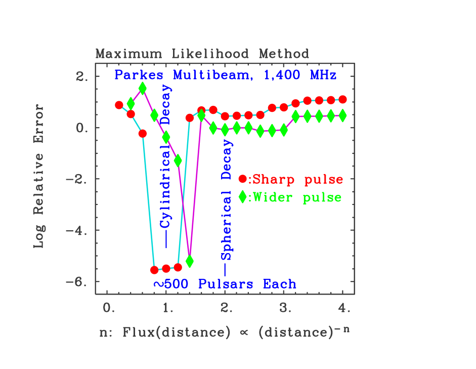
Figure 2: The Maximum Likelihood Method of [EEP, ] as applied in [MLM9, ] to the Parkes Multibeam Survey pulsars without any filtering, and then to the half of that sample whose pulse widths are less than 3% of their pulse periods.

This model also predicts that the emitted power will obey a 1/distance law for two opposite spin latitudes on the sky, which approach, at large distances, $\pm\arccos(\mathrm{c}/v)$, where c is the speed of light, and $v=\omega R>\mathrm{c}$ is the velocity of the update of the circumferential polarization current pattern. At these latitudes, the curve of the Observer time as a function of Source time is cubic, i.e., there is a point of inflection for one (periodic) value of Observer time, where extended ranges of Source times map onto any small interval centered at these Observer times (Fig. 2 of [H98, ]). As a result, a single, very sharp peak appearstwo in the observer’s pulse profile when near that time/phase (see the lowermost curve in Fig. 1). Thus, for any given pulsar,wind observers can tell when they are at, or near, one of these two favored latitudes by the pulse profiles that they record. At more equatorial latitudes, the single pulse splits into two separate pulses, while at more polar latitudes, the single pulse broadens and weakens (the top curve of Fig. 1). See also Fig. 2.10 of [ACS, ].

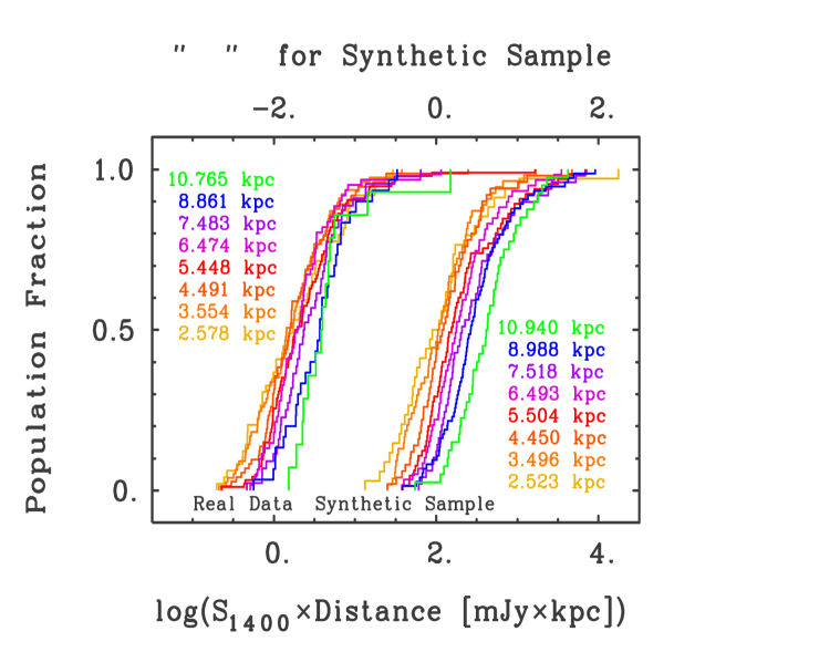
Figure 3: From [M12, ]. Left, lower horizontal axis: the cumulative populations of 497 pulsars from the Parkes Multibeam Survey with pulse widths less than 3% of their periods, which fall into binned distances with centers between $\sim$2 and $\sim$11 kpc, plotted against the log of the product of their 1400 MHz fluxes and their NE2001 distances from [Cordes02, ] and [Cordes03, ]. The spread of the different flux-times-distance products at a given population fraction diminishes as their components become more luminous (and less detection- limited), indicating a 1/distance law. Right, upper horizontal axis: the same for a synthetic population of pulsars whose fluxes obey the inverse square law, and the spread in the flux-times-distance products does not diminish (but would collapse for flux-times-distance- squared products). The two families of curves are both in order of increasing distance from left to right at a population fraction of 0.2.

In the section that follows immediately (Section II), new evidence is added to the old for the effects of supraluminally induced polarization currents in pulsars. Section III derives the 3-dimensional path of the focused beams produced by circularly supraluminal excitations, and discusses their mathematics. Section IV continues with a few more mathematical notes. A discussion of polarization effects follows in Section V.

Section VI discusses the implications for known pulsars, and then describes how annuli of induced polarization currents throughout a large star produce focused beams which break the stellar surface very close to its rotational poles. This section then describes the implications, drawn in [M12, ] from early photometric data of SN 1987A, about the interpenetration of the near polar focused beams through circumstellar material.

Section VII discusses distance effects in pulsars, GRBs, AGN jets, and binary few-million solar mass black holes. Section VIII discusses GRBs as a result of other kinds of supraluminal excitations, deriving redshifts from their afterglows, related effects of NS-NS and BH-NS mergers, and the possibility of focused gravitational beams. Section IX gives a general discussion of supraluminal excitations and focused beams and their effects on pulsars, supernovae, the Sun, Hercules X-1, and other objects. Section X concludes.

II Old and New Evidence

Evidence for this effect in the Parkes Multibeam Pulsar Surveypksmb was first presented in 2009, but a more recent attempt by another groupSD2016 to duplicate the results, based roughly on the same Maximum Likelihood Method (MLM – [EEP, ]) employed in 2009, failed to find the effect. The “Stepwise” MLM does not rely on a simple functional form for the luminosity function, $\phi$(L), but instead iteratively determines $\phi_{\mathrm{k}}$ for the k^th equal step in luminosity. It defines the logarithm of the likelihood function by the logarithm of the sum (over all sources) of the logarithms of the $\phi_{\mathrm{k}}$ every time a source falls into the k^th luminosity bin, minus, the sum (over all sources) of logarithms of, a sum over all $\phi_{\mathrm{j}}$ for all the j^th luminosity bins above the minimum luminosity defined by an unspecified function of the redshift of the source. The inner kernel of this subtracted term is also multiplied by the width of all the steps in luminosity, $\Delta$L, for dimensional consistency. A constraint is also added with a Lagrange multiplier.

Needless to say, the adaptation of such a method, more appropriate to clusters of sources, than to pulsars within the Milky Way disk, is non-trivial. This more recent study of [SD2016, ] included only the $\sim$half of those pulsars in the sample with pulse profiles whose peak widths were greater than 3% of their pulse periods,3 unlike those in the bottom curve in Fig. 1, and in doing so used pulsars for which there was no expectation of a 1/distance law. The 2009 study only excluded these after submission. The results for this restricted sample of 497 pulsars were much more dramatic, as can be seen in Fig. 2. A good guess as to the source of the disagreement is the difference in the number of bins chosen, with the smaller number being more desirable to show the effect in a limited data set, as can be seen in Fig. 3, where cumulative populations were made for eight different subsets over a factor of four in distance. Meanwhile, it is far more important to establish the validity of the violation of the inverse square law independently of the binning issues of the MLM. If need be, the sets from Fig. 3 used in the MLM method will likely reproduce the result of Fig. 2.

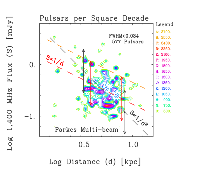
Figure 4: A contour plot of 577 pulsars from the Parkes Multibeam Pulsar Survey whose pulse profiles consist of a single sharp peak with a half width in time less than 3.4% of the period ($\mathrm{F0}\times\mathrm{W50}<34$). The numerical slope of the two parallel dashed lines (red and orange) is -1, corresponding to a 1/distance law, while that of the steeper dashed line (black) is -2, corresponding to an inverse square law. The arrows show what the span of the luminosity function would be if the opposite pairs were appropriately centered (which the red arrow pairs are – slope of -1 – and the black pairs are not – slope of -2).

It is actually easy to show that the narrow-pulse-profile-restricted sample trends toward a 1/distance law as the pulsar fluxes times distances increase above the detection-limited values below 2 mJy-kpc (see Fig. 3). While the mJy-kpc spread of the curves of the actual data sample (at the left) trends toward zero at high mJy-kpc/population-fraction, a signature of a 1/distance law, the synthetic sample (at right), formulated from an inverse square law, retains its spread of $\sim$0.6 (a factor of 4 between 2.5 and $\sim$10 kpc) since it would require multiplication by another factor of distance to collapse.

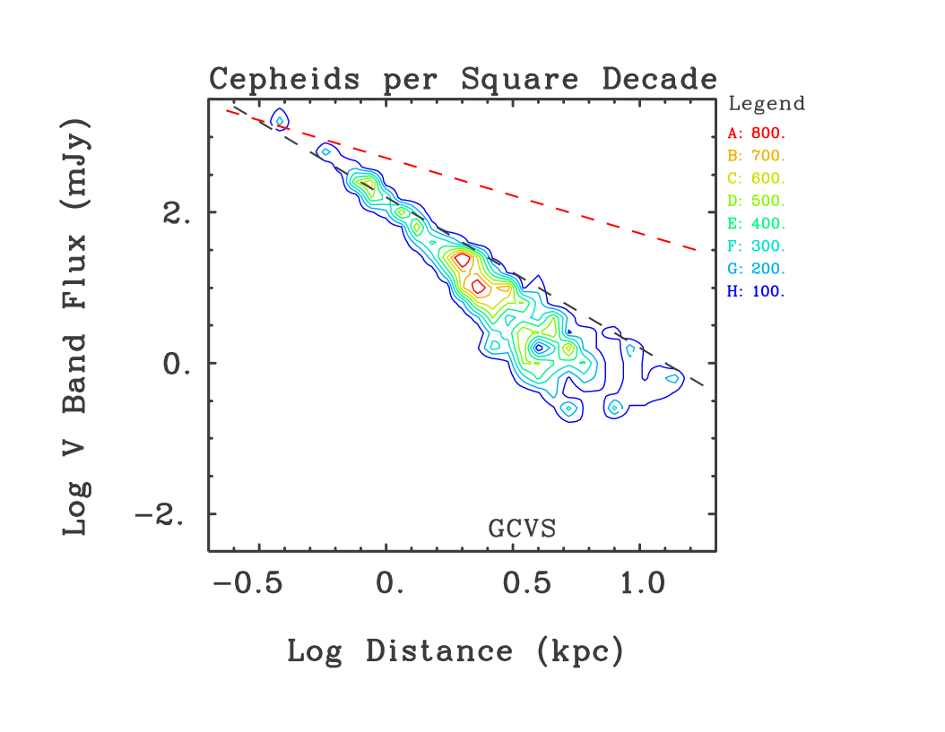
Figure 5: A similar contour plot of 407 Cepheid variables. The numerical slope of the (mostly upper) dashed line (red) is -1, corresponding to a 1/distance law, while that of the steeper line (black) is -2, corresponding to an inverse square law. The Cepheids actually track slightly steeper with distance than a power law of -2, a sign of interstellar extinction.

The population is dense enough (Fig. 4) so that its upper cutoff (orange dashed line) on a log flux-log distance graph follows a numerical slope of -1 well, and a slope of -2 poorly, lying below/above the steeper (black) line at small/large distances. The black arrows show that the inverse square law line does not cut through the same fraction of the luminosity function in the way that the 1/distance law (red arrows) does well. This conclusion is susceptible to having larger populations near one of the two extremes of distance as opposed to mid-distances, but this is clearly not the case, however, as the densest part(s) of the distribution are located at mid-distances. Indeed, it is remarkable how well this distribution’s upper boundary follows a 1/distance law, in spite of it not having been corrected for its denser population at mid-distances. By its very nature, Fig. 3 does not suffer from this problem.

We can check this contour-plotting method on other objects which are known to follow an inverse square law, by analyzing its response to the Cepheids in our Galaxy. Named after the variable star, $\delta$ Cephei (the fourth brightest star in the constellation, Cepheus – “the King”), the Cepheids are massive stars whose period of variability has a near linear relationship to their luminosity. Thus, once we know the interstellar extinction along the line of sight to the particular Cepheid (see, e.g., [amores, ]), we can infer its distance from the difference between its absolute and apparent magnitudes. Figure 5 confirms the contour plot reflects an inverse square law for the Cepheids.

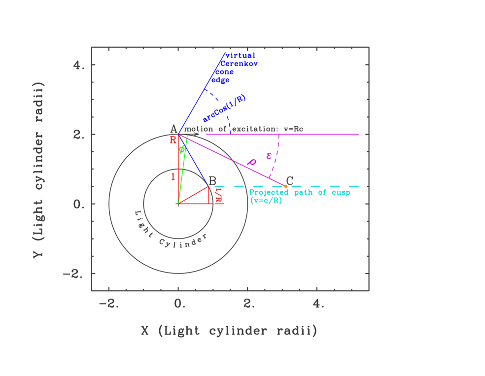
Figure 6: The geometry of circularly supraluminal motion. The instantaneous velocity of $R$ times the wave speed (of light or some other propagating wave) is in the +X direction at point ‘A,’ $(X,Y,Z)$ = (0,$R$,0). The variable, $\phi$ measures the clockwise angle along the circle of radius $R$. The virtual Cerenkov cone, whose axis is parallel to the X axis, but displaced in Y by $+R$, is viewed from above the X-Y plane of the graph, so that its edges form the upper line from point ‘A’, and the lower line from ‘A’ to ‘B,’ on the circle where the rotation of angle due to the motion on the $R$-circle is exactly the wave speed (i.e., the “Light Cylinder” when extended normal to the X-Y plane). The dashed line at $Y=1/R$ is the projection onto the X-Y plane of the (hyperbolic) path of the cusp generated by the supraluminally updated polarization currents near point ‘A’.

III How and why the inverse square law is violated

Supraluminal excitations may result in a focusing of an increasing, extended interval of Source time onto a small interval of Observer time, provided the excitation is accelerated.Lilly Any circular excitation of constant speed is always accelerated toward the center of its circle (see Fig. 6). If there is to be any focusing of such a supraluminal excitation (a point source polarization current traveling in a circle), the focus must lie on the cone whose apex coincides with the source, with its axis, and opening, colinear with the instantaneous direction of motion, and whose half angle is given by $\arccos(\mathrm{c}/v)$, where c is the speed of light (in whatever medium) and $v$ is the speed of the excitation. This opening angle is the compliment ($\arcsin(\mathrm{c}/v)$) of that of the usual Cerenkov cone. For convenience, we will label this as the “virtual Cerenkov cone,” or “vCc.”

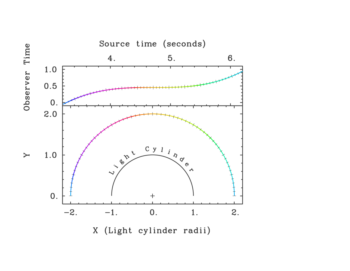
Figure 7: (Lower frame) As in Fig. 6, the geometry of circularly supraluminal motion. The instantaneous velocity is clockwise – in the +X direction at the top of the outer (colored) circle with minor/major tick marks every 3/15 degrees. (Upper frame) The color-coded contributions, of polarization currents in the outer circle/annulus of the lower frame, for a pulsar with a period of $2\pi$, to the Observer time vs. Source time curve (which is also plotted in Fig. 10, in green).

Any temporal information in a part of the source that travels toward the observer at the speed of light and with zero acceleration collapses onto a single arrival time, as can be seen in Fig. 7. The projected separation of the sources along the line of excitation is preserved in the outgoing wave, but the lessening distance penalty for perpendicular offset reduces the difference in their arrival times at increasingly greater distance. The same mechanism for acoustic waves is responsible for the “Sonic Boom.” Centripetal acceleration of the sources toward the center of a circle will always, for the right radius, do better than the Sonic Boom, as we will see below. On the other hand, if the observer is not on the vCc of the excitation, the effects of many nearby sources on the path of excitation will arrive at different times, no matter what the distance.

The virtual Cerenkov cone of circular motion at $R$ times the wave speed in the medium will always have a point tangent to the smaller, concentric circle with a radius, $R_{\mathrm{LC}}$, where the angular motion of $\omega$ radians per second corresponds to exactly the wave speed, or $\omega R_{\mathrm{LC}}=\mathrm{c}$ for electromagnetic radiation. Extension of this circle in the directions of its normals becomes the “Light Cylinder.” For convenience we will use dimensions so that $R_{\mathrm{LC}}=1$. The actual units may be re-established by multiplying the constants, including functions of $R$, by powers of $R_{\mathrm{LC}}$ to make their units consistent, within each equation, with those of the powers of the variables, $X$, $Y$, and/or $Z$, each of which has units of length.

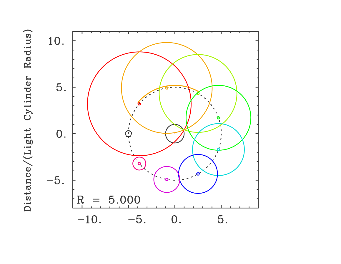
Figure 8: A series of nine Huygen’s wavelets produced by an excitation ending at the left part of a circular path (pentagon) having moved clockwise at five times the wave speed around the circle. The sources from 10 h 20 m to 1 o’clock (an 80^∘ span – highlighted by the orange arc) all contribute to the focus just past 2 o’clock on the circle of radius 1.

With the help of Fig. 8, which has a tangent point on the $R~{}=~{}1$ circle at   21.^∘5 ($\arccos(1/5)=11.^{\circ}537,+10^{\circ}$ from the point at 11 hr 40 min being 20 min short of 12 hr) we can see that the tangent point ’B’ in Fig. 6 ($30^{\circ}$ for $R=2$ on the small circle) is likely the first point of the focus curve we are seeking. If we start with a point ‘A’ on the X-Y plane at (0,$R$) in Fig. 6, where the supraluminal excitation is traveling at $R$c in the +X direction (i.e., rotating “clockwise”), the vCc appears in profile, with its axis parallel to the X axis. This cone is tangent to the light cylinder at point ‘B’:

$$(X,Y,Z)=(\sqrt{1-{1\over R^{2}}},{1\over R},0),$$ (1)

and in consequence the line from ‘A’ to ‘B’ coincides with the lower edge of the vCc. The equation for this line is:

$$Y=-(\sqrt{R^{2}-1})X+R,$$ (2)

and we will need it to relate an arbitrary point at ($X$,$Y$), to the right of point ‘B’ in Fig. 6, to the hyperbola on the vCc at the given $Y$ value, in order to solve for its $\pm Z$ values. Given the $Y$ value, the $X$ solution to Eq. 2, $X_{o}$, is the $X$ fiducial in the equation for the corresponding hyperbola on the vCc which returns the value for $Z$:

$$Z=\pm\sqrt{R^{2}-1}\sqrt{X^{2}-{X_{o}}^{2}}~{};~{}X_{o}=(R-Y)/\sqrt{R^{2}-1}~{}.$$ (3)

In order to find the exact path which will mark the location of the cusp/focus on the vCc (or confirm that it is an hyperbola), we must compute the distance, $\rho$, from a point on the $R$-circle near ‘A’ to the cusp/focus point on the vCc, as a function of $X$, and $Y$, for a range of angles, $\phi$ (Fig. 6), on the $R$-circle, and test for a $\rho(\phi)$ function that changes by only a small fraction of a light-radian over a large range in $\phi$ (of up to a radian), which is exactly what we need to get many Source times mapped into one, or a limited range of, Observer time. Thus, starting at an arbitrary point on the $R$-circle near ‘A’, at phase $\phi$, or $(R\sin{\phi},R\cos{\phi},0)$, and computing the distance to near point ‘B’, or ($\sqrt{1-1/R^{2}}$,$1/R$,0), we get:

$$\rho(X,Y,\phi)=((RX)^{2}-2RX\sin{\phi}+2RY(1-\cos{\phi}))^{1/2}.$$ (4)

We notice that terms in $Y^{2}$ and others that do not multiply trigonometric functions of $\phi$ have vanished, leaving a simple $Y$ dependence for the factor, $(1-\cos{\phi})$.

By removing a factor of $RX$ from the square root and after using the binomial expansion for the 1/2 power, we get:

$$\rho\sim RX~{}(1-({{\sin{\phi}}\over{RX}})+{{RY}\over(RX)^{2}}(1-\cos{\phi})-{1\over 2}(\cdots)^{2}+\mathrm{higher~{}terms}),$$ (5)

where the ‘$\cdots$’ represents the grouped terms following the initial ‘1’. A factor of 1/4 from the binomial expansion coefficient has been absorbed by the choice of ‘$\cdots$’ when squared. The first term, $RX$ after multiplying through the parenthesis to the ‘1’, represents the macroscopic distance to the location of the beam focus.

The -$\sin{\phi}$ in the next term expands (in radians) initially to $-\phi$, i.e., the distance, $\rho$, is less for higher positive $\phi$ values, which advance any excitation near point ‘A’ in Fig. 6 to higher $X$ toward the right and the observer/beam focus. This ‘$-\phi$’ cancels the delay of the source rotation on the $R$-circle, on which motion toward positive $\phi$ costs time, allowing many source points on the $R$-circle to nearly simultaneously affect one observer point. However, since Eq. 5 is an approximation, an error in this linear term in $\phi$ with a magnitude which is inversely proportional to distance is always present, and in consequence prevents any signal from becoming infinite while producing the 1/distance law.

The next term in the expansion of the $-\sin$ is ${\phi}^{3}/6$. This cubic term has been mentioned above, and its slow departure from 0 near $\phi=0$ would lead to an infinite response at one particular Observer time for every cycle, if it were not for the residual linear term in $\phi$.

We can see how the infinity would be generated by estimating the response at the observer position, which, is how much Source time (essentially $\phi$, in radians) gets mapped into a small interval of Observer time. In effect, the response is the derivative of Source time as a function of Observer time. If high, then a large interval of Source time maps onto a small interval of Observer time. Our $f(\phi)={\phi}^{3}/6$, as shown by the bottom curve in the left hand frame of Fig. 1, however, is the Observer time as a function of Source time – the inverse of the function we need. We must turn the function on its side, as Fig. 1 suggests. Thus we need the derivative of $\phi(f)$:

$$\phi(f)=(6f)^{1/3}.$$ (6)

Differentiating we get:

$${{\partial\phi(f)}\over{\partial f}}=2^{1/3}(3f)^{-{2/3}},$$ (7)

which is infinite for $f=\phi=0$.

Continuing, there are more terms from the ‘$1-\cos(\phi)$’, of which the lowest one is, when multiplied by the leading $RX$,

$${RY\over 2{RX}}{\phi}^{2},$$ (8)

and a similar term,

$${-{\phi}^{2}\over 2{RX}},$$ (9)

comes from the ‘$\phi$’ part of the ‘$\sin$’ term in the ‘$-{1\over 2}(\cdots)^{2}$’ continuation of the binomial expansion. If $Y=1/R$, the same value as the $Y$ for point ‘B’, these terms cancel completely, and permanently if $Y$ stays at $1/R$, as do the factors which do not multiply functions of $\phi$.

Thus the focus, which starts at $Y=1/R$ at point ‘B’, is always at $Y=1/R$. The next higher term in $\phi$ also comes from two contributions, and for $Y=1/R$, after multiplying through by the leading $RX$, amounts to

$${{\phi}^{4}\over{8RX}},$$ (10)

which, because it is a higher power than the cubic, and decreases with distance, is not important.

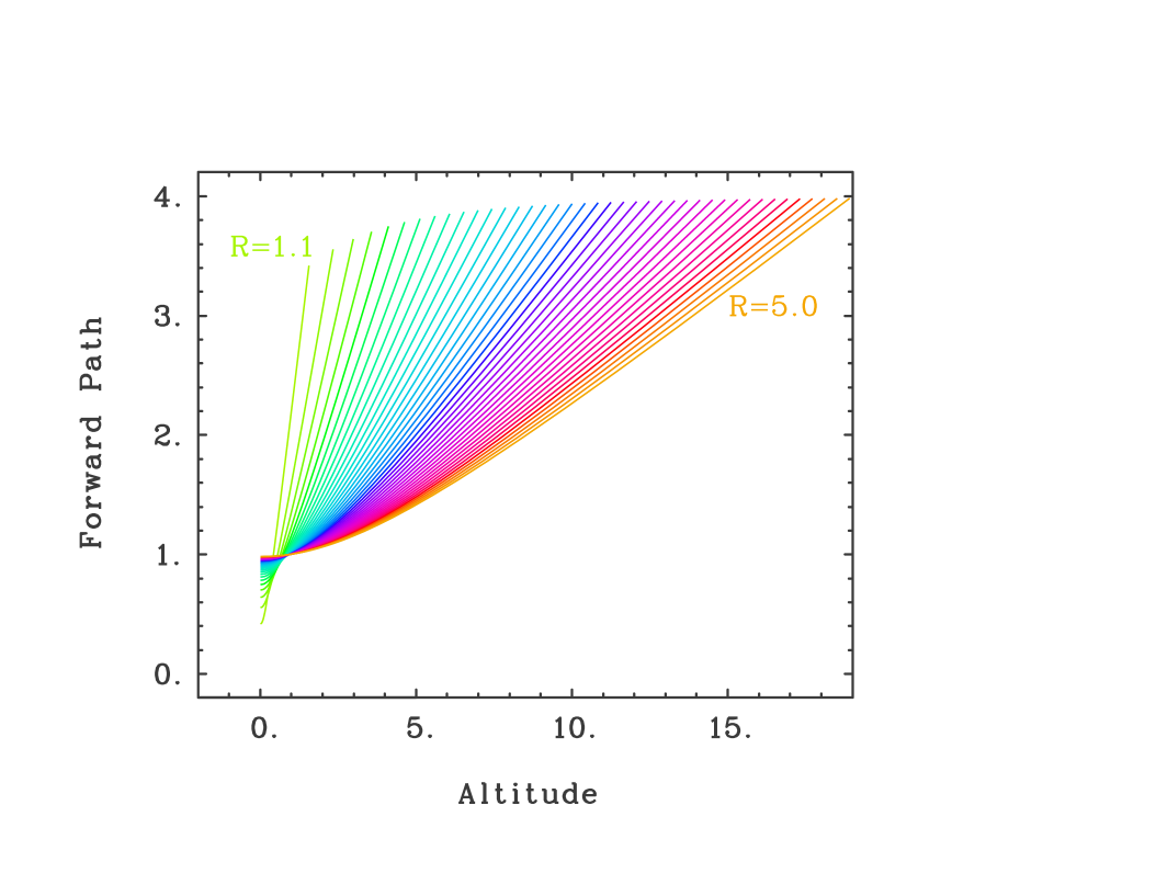
Figure 9: Curves of the path of the cusp plotted in the Z-X plane for $R=1.1~{}\mathrm{to}~{}5.0$ in steps of 0.1.

Since the Y value for the path of the focused beam remains at $1/R$ out to infinity, the equation for the focused beam on the vCc is an hyperbola which is simple to express:

$$Z=\pm\sqrt{R^{2}-1}\sqrt{X^{2}-1+{1\over R^{2}}};~{}Y={1\over R}.$$ (11)

Figure 9 plots these curves in Z-X for $R=1.1~{}\mathrm{to}~{}5.0$.

We can see how an error in the linear term in $\phi$, call it $\varepsilon\phi$, where $\varepsilon$ is the small angular value from Fig. 6, affects the pulse profiles when included in the contributions, as has been done in Fig. 10 for a distance of $200\pi$, with $\varepsilon=0.05$ at this distance, and dropping as 1/distance for the remaining $400\pi$ and $600\pi$. The peak heights of the pulse profiles of this figure do, in fact, represent a 1/distance law. The actual value for the linear error coefficient multiplying $\phi$ is orders of magnitude smaller, and numerically challenging to compute at sufficiently high resolution to show the effect, as we will see in Fig. 11. No matter how small this effect, however, it will produce a 1/distance law.

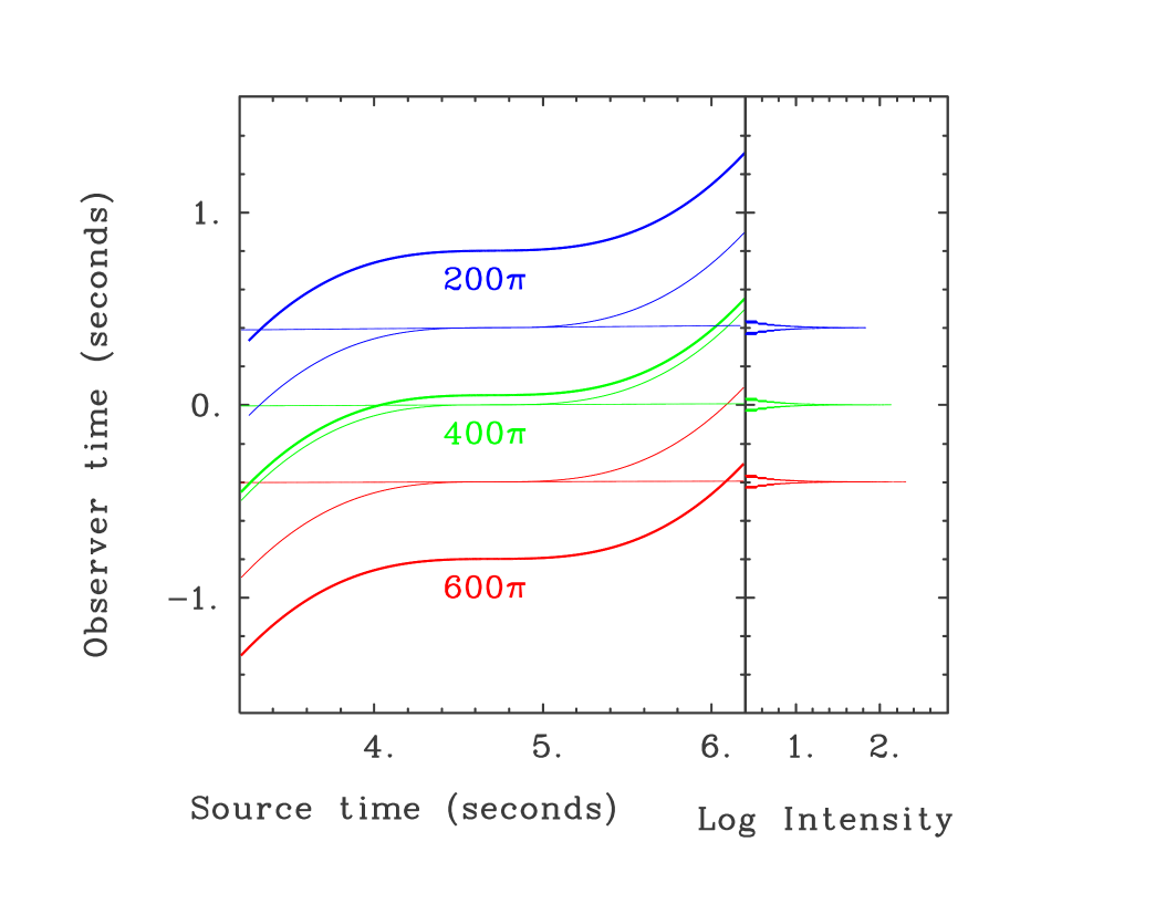
Figure 10: Observer time as a function of Source time curves for a simulation of a pulsar with a period of 2$\pi$ and plasma at $R=5$, for three different distances, $200\pi$ (top two [blue] curves), $400\pi$, (middle [green] curves), and $600\pi$ radians (bottom two [red] curves), with the inverse square dependence removed. (Unlike Fig. 6, a coordinate system, where $\phi=0$ corresponds to the X-axis, has been used – hence the flat sections of the curves occur at $1.5\pi$). The three straight lines plot the product, $\varepsilon\phi$ for the three distances (where $\varepsilon$ has been arbitrarily set to 0.05 at $200\pi$, and drops as 1/distance as does that defined in Fig. 6. The topmost and bottommost curves represent the sum of the original curves and the lines (the same holds for the middle curve, only with a smaller offset to the sum curve – this curve is also plotted in Figure 7).

With no distance law incorporated into the three sum curves in the right hand frame of Fig. 10, the more distant (red/lowermost) peak is 0.5 logarithmic units higher than the (blue/uppermost) peak which is three times closer, exactly compensating an inverse square law (when applied) to a 1/distance law. As long as the sampling over Observer time is kept sufficiently fine, and that over Source time is done likewise to maintain a sufficiently large sample to produce the pulse profiles in the right-hand frame, there is no contribution too small to produce this effect, again because the pulse profiles are otherwise infinitely narrow. Sixteen million plus points were needed, across the vertical of the right hand frame in F Fig. 10, to reveal the 1/distance law for a modulation of $0.001~{}\varepsilon(20\pi,40\pi,60\pi)~{}\phi$ (or $\varepsilon\phi$ for distances of $20,000\pi$, $40,000\pi$, and $60,000\pi$). Half as many points led to an effect which matched the 1/distance law poorly, whereas twice as many points led to a quantitatively excellent fit.

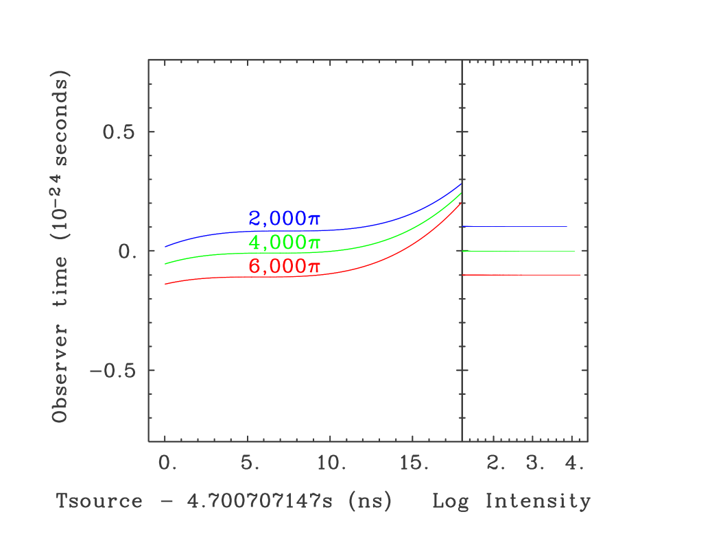
Figure 11: Observer time as a function of Source time curves for an actual pulsar with a period of 2$\pi$ and plasma at $R=5$, for three different distances, $2,000\pi$ (top [blue] curve), $4,000\pi$, (middle [green] curve), and $6,000\pi$ radians (bottom [red] curve), and, as with Figure 10, the inverse square dependence removed. (Unlike Fig. 6, a coordinate system, where $\phi=0$ corresponds to the X-axis, has been used – hence the flat sections of the curves occur at $1.5\pi$).

Calculations were also done for a pulsar of period $2\pi$ at distances of $200\pi$, $400\pi$, and $600\pi$ down to Source time range of $\sim$10 ns and increments $<10^{-15}$ s and an Observer time range of a small fraction of $10^{-25}$ s. By fine adjusting the distances by parts per 10 billion, the centering effects of the peaks could be dithered. Although the responses at distances of $600\pi$ and $400\pi$ were essentially a “dead heat” after compensating for the inverse square law, the response at $200\pi$ was down by 22% – the first noticeable manifestation of an inverse square law violation. By contrast, the result of calculations done with distances of $20\pi$, $40\pi$, and $60\pi$, produced the strongest signal, removing the inverse square dependence, at the smallest distance, $20\pi$. With a factor of fifty decrease in Source time range for the $100$’s of $\pi$’s calculations, and a similar factor of 10,000 in Observer time, the $\pm 10^{-31}$ s resolution of this time in the 128-bit double precision becomes apparent.

When doing these calculations, it was important to use an Observer time resolution sufficiently small to prevent contributions of one distance splitting into two neighboring pulse profile bins, which caused the results to vary much more widely. When adjusted, the small Observer time range of the actual peaks would almost always fall into a single bin, with the pattern, of a fixed number of adjacent empty bins between those with (continuous) content, persisting for hundreds of consecutive bins.

Further calculations were done for distances of $2,000\pi$, $4,000\pi$, and $6,000\pi$. The Source time resolution was $2.2\times 10^{-14}$ s, and the Observer time resolution was $1.9\times 10^{-31}$ s, and the effects shown in Fig. 11 are much more robust, producing about half (on average, but more for the example plotted) of the logarithmic difference needed for a 1/distance law. Calculations were also done for distances of $20,000\pi$, $40,000\pi$, and $60,000\pi$, with no real increase in the range of responses, likely due to the larger distance range causing the Observer time to hit the double precision limit for coarser resolutions.

The full effective timing advance/delay of the focused beam at distance, $f(\phi)$, as a function of $\phi$ at increasing distances becomes the sum of all terms,

$$f(\phi)={\phi^{3}\over 6}+\varepsilon\phi+\mathrm{Constant},$$ (12)

and the constant is absorbed into the macroscopic distance. This relation can be rewritten as a standard cubic equation,

$$\phi^{3}+6\varepsilon\phi-6f=0,$$ (13)

which has the standard solution:

$$\phi=(3f+(8\varepsilon^{3}+9f^{2})^{1/2})^{1/3}+(3f-(8\varepsilon^{3}+9f^{2})^{1/2})^{1/3}.$$ (14)

To get the maximum peak height we differentiate this wrt $f$ and set $f=0$. The result is:

$$({\partial\phi}/{\partial f})_{f=0}=1/\varepsilon.$$ (15)

Thus if, with an increase in distance, the slope of the linear term in $\phi$, $\varepsilon$, decreases by the same relative measure, then, in consequence, a greater range of the $R$-circle contributes to the same, narrow width of the pulse. Starting with a very small range of contribution in $\phi$, this can continue until almost two radians of the R-circle contribute, when the changing polarization limits further contributions (see Section V). Even when this happens, the same range of $\phi$ contributes to an increasingly narrow pulse width in Observer time as distance increases. So although the pulse height is restricted, beyond this point, to an inverse square law, the narrowing of the pulse represents that much more energy from its increasing range of Fourier components, thus the energy of the pulse still obeys a 1/distance law. This is known as “focusing in time.”

More quantitatively, if we let $\delta$ represent a small interval/distance within the pulse profile that the observer sees, then there will be some $\phi_{limit}$ which represents the contribution of source from the $R$-circle whose energy falls within that $\delta$ for the observer:

$$\delta={{\phi_{limit}}^{3}\over 6}+\varepsilon\phi_{limit},~{}~{}~{}~{}~{}\textrm{(in radians)}.$$ (16)

Multiplying this equation by $R_{LC}$ restores the original units of distance, as in the first term of Eq. 4, the square root of distance squared. Then dividing by c converts this into an equation involving time. It can then be converted into radians by multiplying by the rotation frequency, $\omega$. These three factors cancel exactly by definition, so Eq. 16 involves radians, and needs no conversion.

Given that $\phi^{3}/6$ is small, we get $\phi_{limit}=\delta/\varepsilon$. The resulting pulse profile will be a single sharp peak of a certain, narrow width, $\delta$, at least until $\phi_{limit}$ approaches $(6\delta)^{1/3}$. Setting the two contributions equal, we get an equation for $\delta$ in terms of $\varepsilon$: $\delta=\sqrt{6}{\varepsilon}^{3/2}$, which gives the upper limit to $\delta$ above which the further contributions of source on the $R$-circle will be limited, unless $\delta$, and hence $\varepsilon$, are reduced, so that the 1/distance response can continue for greater ranges. We will continue to explore this in Section VII.

IV Further Considerations

The equation for $\rho$, now that we know $Y=1/R$, and $Z(X,R)$, is:

$$\rho(X,R,\phi)=[(R\sin(\phi)-X)^{2}+(R\cos(\phi)-1/R)^{2}+(R^{2}-1)(X^{2}-1+1/R^{2})]^{1/2}.$$ (17)

If we differentiate this wrt time, and set $\phi$ to 0, it simplifies drastically to:

$$\rho(X,R,\phi=0)=XR.$$ (18)

And if we use the fact that $d\rho/dt=\textrm{c}$, it follows that:

$${dX\over dt}=\textrm{c}/R,$$ (19)

and this is even true (on average) between $X=0$ and $\sqrt{1-1/R^{2}}$.

The velocity of the focus, on the other hand, is infinite and diverging in the Z direction at $Z=0$, and becomes finite at $Z\neq 0$, but remains greater than c, even if ever so slightly, for the rest of its path to infinity. Causality is not violated since the path is not a straight line. Also, because the path of the focus is not radial from the contributing currents on the R-circle, the elements making up the focus represent parts of their spherical emission which change continuously as the focus moves outward. But although these paths also curve over toward $+X$, once $Z$ is no longer 0, the progressive narrowing of the vCc’s caused by the extreme deceleration prevents any secondary focus from forming. The focus we’ve discussed is the only focus for circularly supraluminal excitation.

We can derive the distance scale of change for the angle, $\varepsilon$ (not restricted to the X-Y plane) by taking the cross product of the vector to the source of excitations, $(0,R,0)$, with the $\rho$ vector: $(X,1/R-R,\sqrt{R^{2}-1}\sqrt{X^{2}-1+1/R^{2}})$, and then dividing by the moduli of the two vectors, namely $R$ and $RX$ respectively. This quotient will yield the value of $\cos(\varepsilon)$, which for great distances will be slightly less than unity. The cross product is $(R\sqrt{R^{2}-1}\sqrt{X^{2}-1+1/R^{2}},0,-RX)$, and the quotient is:

$$\cos(\varepsilon)=1-{1\over X^{2}}(1-1/R^{2})^{2}.$$ (20)

At great distances we can estimate $\varepsilon$:

$$\varepsilon={{R-1/R}\over{\rho}};~{}\textrm{where}~{}\rho=RX.$$ (21)

as we might have guessed.

So far we have discussed the situation involving just a moving point source of emission, whereas in the real world volume sources are involved, and issues such as plasma screening rear their ugly heads. However, pulsars really do obey the 1/distance law we’ve discussed here, so there must be some way that pulsar emission can act like a lot of point sources, possibly by field lines bunching together, as suggested by [Contopoulos, ]. Temporal structure as short as 0.4 ns [HE07, ] has been observed in the giant pulses of the Crab pulsar, yielding a range in timescale close to 80 million (33 ms/0.4 ns). However, we will see in Section VII evidence for a range close to the square of this factor.

V Polarization

The polarization of all sharp pulsar peaks observed in the Universe swings from nearly $+\pi/2$ to $-\pi/2$ across the pulse (or vice-versa – see, e.g., Fig. 2 of [MP87, ]), and this can be understood from Figs. 6 and 7, as the source time of the pulse moves across a macroscopic range.

For any given electric field element in the X - Y plane, $V$, with components $(V_{x},V_{y},0)$, there is a polarization field, $W=(W_{x},W_{y},W_{z})$, for the direction, $\rho=(\rho_{x},\rho_{y},\rho_{z})$, which has to be perpendicular to $\rho$, and lie in the $\rho-V$ plane. So we have ${W\bullet\rho}=0$, and $W\bullet(V\otimes\rho)=0$. There is a penalty for the angle between $V$ and $W$, which is just the dot product between the two, once $W$ has been determined, as described below.

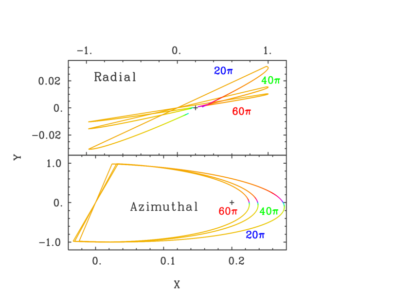
Figure 12: The X and Y offsets from the Z axis for a unit vector derived from the cross product of the polarization vector with $\rho$ at phase $3\pi/2$ (in a right-handed coordinate system, i.e., “approaching”), for a pulsar with a period of $2\pi$ seconds and plasma at $R=5$, for distances of $20\pi$, $40\pi$, and $60\pi$ light-radians. Loci for polarizations resulting from an electric field vector of $(\cos{\phi},\sin{\phi})$ (radial), and $(-\sin{\phi},\cos{\phi})$ (azimuthal) are plotted in the bottom and top frames. The color coding of the loci is the same as for Fig. 7.

For a radial electric field, $V=(\cos({\phi}),\sin({\phi}))$ (in a right-handed coordinate system with $\phi=0$ for the +X axis), and using $W\bullet\rho=0$ to substitute for $W_{x}$, we get:

$$W_{z}=W_{y}\rho_{z}(V_{x}+V_{y}\rho_{y}/\rho_{x})/(V_{x}\rho_{y}-V_{y}({{\rho_{z}}^{2}}/\rho_{x}+\rho_{x})).$$ (22)

By using $({W_{x}}^{2}+{W_{y}}^{2}+{W_{z}}^{2})=1$, all three components of $W$ are determined. For an azimuthal electric field, $V=(-\sin(\phi),\cos({\phi}))$, when substituting for $W_{y}$, we get the same equation with subscripts ‘x’ and ‘y’ exchanged. The loci of these $W$s, in the plane of the $Y$ direction and that perpendicular to the X-Z asymptote ($Z=\sqrt{R^{2}-1}X$), are simple to describe.

The results for both the radial and azimuthal cases are shown in Fig. 12. Polarization offsets with magnitudes inversely proportional to distance are present in both orientations. More importantly, however, is the fact that the angle of polarization swings drastically during the period of maximum response, as is both predicted and observed. Although the residual offset of the points from (0.2, 0.) in the lower frame, and the residual slope of the curves in the upper frame approaches 0., a residual slope does persist in the linear parts of the curves in the lower frame.

In addition, when constructing a closer ns-scale Source time counterpart to Fig. 10, points at distances of $10\pi$, $20\pi$, and $30\pi$ would have to be retarded in phase by 0.02122, 0.03183, and 0.06364 radians, respectively, in order to have their inflections coincide, on the ns scale, with $1.5\pi$, an effect presumably due to approximation errors and/or higher order than cubic terms of the expansion of Observer time in powers of $\phi$, which also have a 1/distance dependence.

Finally, the dot products of the polarization vectors with their $\phi=0$ (as in Fig. 6) counterparts are shown in Fig. 13, which confirms they rotate as time progresses, as well as small differences between distances and electric field orientations. In addition, Fig. 13 confirms the above statement that the points of inflection in Observer time as a function of Source time occur at slightly different phases at different distances.

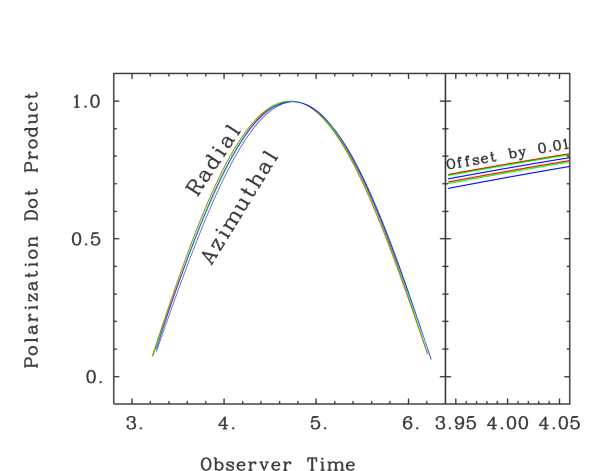
Figure 13: The dot products of polarizations, resulting from radial and azimuthal electrical field vectors on an annulus at $R=5$, with their counterparts at $\phi=0$ (using the convention of Fig. 6), for distances of $20\pi$, $40\pi$ and $60\pi$. (Right frame) A close up of a small section of the curve in the left frame, with the three radial dot product paths offset up by 0.01.

These two figures show, at least for the $R=5$ case, that the polarization vector has significant components of rotation, other than the overall rotation with phase, at $\phi=0$ (as in Fig. 6), for azimuthal and radial surface electric fields, with a rate which is inversely proportional to $\rho$.

VI Implications for known pulsars and supernovae

VI.1 Pulsars

At least half of all known pulsars — those whose pulse profiles consist of a single, sharp pulse of width less than $\sim$3% of their periods — have been discovered because their rotation axes are oriented nearly perpendicular to the line of sight to the Earth. Isolated neutron stars must gravitationally concentrate interstellar plasma in order to emit radiation (via cyclotron emission and/or strong plasma turbulence) mostly in a location outside of the light cylinder, because this region marks the beginning of supraluminally generated focused radiation.

And the place in this region where plasma is most highly concentrated is just outside the light cylinder. For isolated pulsars, this emission occurs atM12 ; Weisskopf $R=1/\cos{4^{\circ}}=1.00244$. This means that the speed of the excitation, $v$, is just slightly greater than the speed of light, c, so that $\arcsin(\mathrm{c}/v)$ is almost $90^{\circ}$ — the cones of favored emission are very open, and the favored emission is very nearly equatorial. This may have observational consequences.

For example, no sustained central source has been detected in any nearby modern SN except 1986J, and, by now, even that source does not appear to be consistent with a strongly-magnetized pulsar remnant.BB17 It is also the only one viewed in the center of an edge-on galaxy, NGC 0891. If the rotation axis of any pulsar remnant is perpendicular to the NGC 0891 galactic plane, then we are close to its favored direction of its emission (4^∘), raising the possibility that the visibility of the central source in 1986J is not entirely fortuitous. The larger the star, the more likely its angular momentum aligns with that of its host galaxy, and all the more so for binary mergers.

The implications of a 1/distance law for pulsar emission, even restricted to exactly two opposite spin latitudes, are far-reaching (to coin a phrase). It is responsible for the continued success of a long string of pulsar searches made over the last several decades. It may be responsible for the utraluminous pulsed X-ray source found in NGC 5907.ULX Although currently, no radio pulsar has been discovered in any galaxy beyond the Large and Small Magellanic clouds, the Square Kilometer Array may change that.ska The nearby galaxy in Andromeda, M31, and another nearby spiral, M33, may yield many pulsars each.

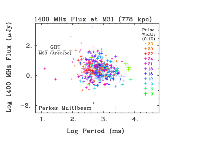
Figure 14: The 1400 MHz fluxes of the 577 Parkes Multibeam pulsars, with pulse FWHMa$<$0.034 cycles, when placed at the distance to M31 (778 kpc), assuming that all obey a strict 1/distance law (and ignoring their individual placings in the Milky Way). The dashed line at the left represents the approximate limit of the NRAO Green Bank Telescope for M31, and that of the Arecibo 300-meter dish for another spiral galaxy, M33, at $\sim$900 kpc (at $41^{\circ}$ declination, M31 is out of reach from Arecibo, but like M33 makes a good target for FASTFAST ).

However, we are not there yet, and care must be taken when making estimates of how far we can go presently. For example, [Rubio-Herrera, ] determined that, if the “most luminous” pulsar in the Galaxy, PSR B1302-64, were placed in M31, it would need to be five times as luminous in order to be detected in a survey using the 12, 25-meter antennae of the Westerbork Synthesis Radio Array. Since M31, at 778 kpc, is 64.35 times farther away than B1302 is from the Earth ($\sim$12 kpc), it can be inferred that B1302 was robustly detected at 13 times the threshold level of the survey.

However, B1302 is only the most luminous pulsar assuming that its flux obeys an inverse square law within the Milky Way! With a 571 ms period and a pulse widthscat of 19 ms, B1302 is almost certainly near a 1/distance law, and thus its luminosity is overestimated.

Figure 14 plots what the 1400 MHz fluxes would be at the 778 kpc to M31 for the 577 Parkes Multibeam pulsars whose pulse FWHM is less than 0.034 cycles (so that B1302-64 is included). On this graph the flux of B1302 at M31 is only 25 $\mu$Jy, lower than 21 other pulsars.W1400 With 310/1.8 mJy at 4.5/778 kpc, the sharply pulsed (0.018) B1641-45 is the clear winner at M31. The bulk of the population lies between 1 and 10 $\mu$Jy.

For the Magellanic Clouds themselves, the 59.7 kpc-distant Small cloud has four known pulsars, with pulse widths of 0.0300, 0.0216, 0.0189, and 0.0138 cycles, while the 49.7 kpc-distant Large cloud has 12, with two young, strongly magnetized pulsars at 62 (X-rays only so far), and 20 Hz, both of which were discovered in the X-ray band. It also has 10 more exclusively radio pulsars, with pulse widths of 0.0818, 0.0326, and 0.0246 cycles, and the remaining seven with still narrower peaks — like the SMC a narrower sample than the the full PKSMB — lending support to the pulsar model under discussion.H98 ; Narrow

The 20 Hz pulsar in the LMC (B0540-69.3) has a double peak spanning one third of a cycle (see the middle pulse profile in Fig. 1), characteristic of a viewpoint which is more equatorial than optimum ($4^{\circ}$). The shock(s) of the Chandra image of this pulsar appear as a straight lineSerafimovich ; ch04 consistent with our view being extremely close to equatorial, again lending support to the supraluminal excitation model of pulsar emission.

The 62 Hz pulsar in the LMC, J0537-6910,M06 has a marginally narrow pulse ($\sim$0.1 cycles), which appears to be a close double. Thus our view is farther from the equatorial than it is for B0540, and closer to optimum. Its nearly-aligned magnetic field is drifting toward its spin equator by about a meter per year, but the field strength, rather than effective dipole, is what matters for cyclotron radiation. In the case of J0537, its field is still strong enough, at its close-in light cylinder, to produce X-rays, but few optical photons because the cyclotron process can not produce subharmonics, still another test that the model passes, and few others do.

Similar strongly magnetized pulsars, such as that in the Crab Nebula (30 Hz), may drive winds which move material through positions of favored supraluminal excitations relative to an observer. The Chandra image of the shocks near the Crab pulsarch04 ; Weisskopf show an ellipticity consistent with our view being 29^∘ off the rotational plane, an orientation which would produce the weakest (top) pulse profile shown in Fig. 1 — i.e., the interpulse. The very sharp main pulse (a 1.1 ms FWHM) could be the result of emission from the wind where its material passes through the favored location at $R=1/\cos(29^{\circ})=1.143.$ The absence of the GHz emission bands, seen in the interpulse, is consistent with the less homogeneous environment from which this feature must arise.

Finally, the pulse profiles recorded for the periodic 2.14 ms signalM00 ; M00c from SN1987A were rarely anywhere near as sharp as are at least half of all radio pulsars, with the smallest pulse widths at no less than 10%. Thus it was difficult to reconcile this pulsation with a real source at 49.7 kpc, with a violation of the inverse square law apparently ruled out. The answer, in this case, is that an otherwise sharp pulse is broadened by the phase variation of the precession, for which there is evidence in all of the results sufficiently significant to reveal it.

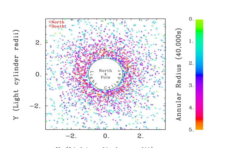
Figure 15: The emergence locations (X-Y, near the northern rotational pole) for the 2,655 focused beams which fall within the (X=$\pm$3.5, Y=$\pm$3.5) radians of the frame out of 3,930 annuli of polarization currents within a post-core-collapse star of 400,000 radians diameter (a 19.08 million km radius for a 500 Hz pulsar, and a 190.8 million km radius for a 50 Hz pulsar). The annuli are spaced in polar depth and radius by about 1,000 radians. Phase lag has been accounted for, making the azimuthal locations for the emergences essentially random. The ‘o’ symbols mark the emergences from annuli in the stellar northern hemisphere, and ‘x’ symbols for those from annuli in its southern hemisphere.

VI.2 Supernova disruption

The 1/distance law is essential to pulsar-driven supernova disruption — the progenitor star radii are in the range of 1 – 40,000 light-periods ($2\pi R_{\mathrm{LC}}$/c), whether white dwarf – white dwarf or blue supergiant, core-merger, $\sim$ 500 Hz pulsars, or solitary red supergiant, $\sim$ 50 Hz pulsars (see Fig. 15). Annuli of polarization currents close to the poles, as well as annuli at all but the smallest radii deeper from the poles, all contribute to beams which are concentrated at the poles.

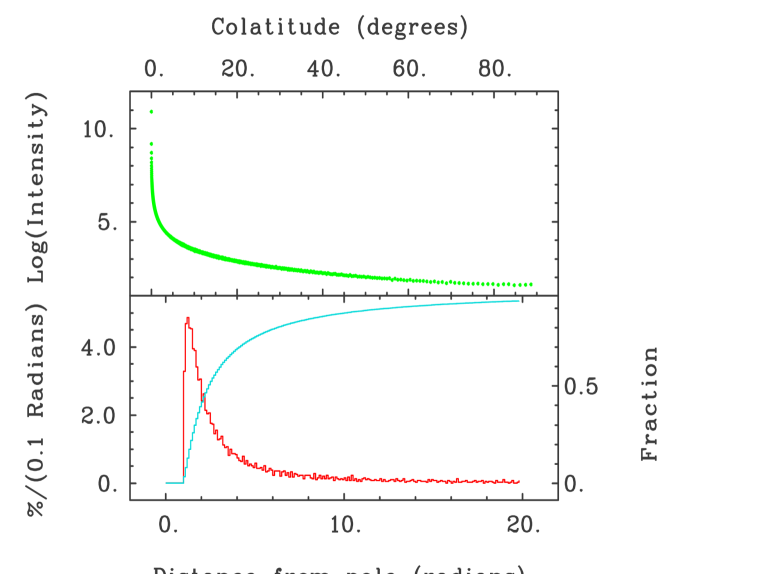
Figure 16: (Lower frame, left hand vertical scale) The percentage of 3,930 cusp emergences (red) histogrammed in steps of 0.1 radians projected polar radius. (Lower frame, right hand vertical scale) The cumulative fraction of emergences (cyan) vs projected polar radius. (Upper frame,left hand vertical scale) The log of the number of cusp emergences, at all azimuths, per degree of colatitude (upper horizontal scale). The highest resolution of 0.01 degrees corresponds to 35 radians in the horizontal scale of the lower frame.

Thus the jets driven from this radiation are polar, emerge within minutes of core collapse, and can be collimated to a high degree,M12 easily one part in 10,000 (see Figs. 15 and 16), and still more for larger stars, making this one of the most anisotropic known processes in the Universe.

The advantage in $1/r^{3}$ dipole strength for the near-axially induced/smaller radius, $r$/more equatorially erupting beams, over the less axial/larger $r$/more polar beams is not as great as might be expected. The contributions to the latter grow larger with $r$, are boosted by a centripetal acceleration which also grows with $r$, and are focused onto the smaller polar rather than the larger equatorial regions. In the end, the excitations/beams to both regions must propagate out of the stellar core and at least the rest of the stellar radius, with the paths from the annuli of greater radii avoiding more and more of the stellar core as they penetrate to the poles.

Thus a plot of the number of beam emergences vs colatitude (upper frame of Fig. 16) may be a decent measure of anisotropy, although no adjustment has been made for the differing stellar densities at the locations of the polarization currents. However, pulsar precession [M00, ; M00c, ] limits the effective anisotropy to about a factor of 100, arguably even less than the collimation ($R\leq 210$) implied by “Bright Spot 2” of [NP99, ], which was roughly the same physical size, but much more distant from SN 1987A. For stars with circumstellar material, a meandering pencil beam cuts through this gas, producing copious amounts of radiation along the way. The amount of radiation produced may be comparable to that which emerges from the poles.

This is not unexpected, considering the SN 1987A “Mystery Spot” or “Bright Spot 1” – a feature observed on days 30 and 38 by [Nis, ], and day 50 by [MMM, ], to be consistent in magnitude ($\sim$6% of the optical flux of the SN proper), position angle ($194^{\circ}$), and, with a reasonable extrapolation, offset (45, 60, and 74 milli-arc seconds, or a few light-weeks south by southeast of the SN proper) – and its anisotropy,WWH visible in the remnant now for the last few decades. For large stars either the core merger process within the common envelope,M18 or the reduction of the core’s moment of inertia through progressive nucleosynthesis, initiatesM this anisotropy even before core collapse.

Early spectra of SN 1987A indicate “bright sources underlying diffuse material,” not unlike glowing pyrotechnic embers viewed through intervening smoke. Much, but certainly not all, of this underlying luminosity must come from the visible South pole. The rest must originate from the effect of the polar jets penetrating their overlaying circumstellar material, which, given the 9-day delay (Fig. 3 of [M12, ]) and the 75^∘ orientation, indicates such material at locations light-weeks above the poles.

Following a small, 1-day increase at day 7.8 due to the UV flash hitting, but not penetrating deeply into, the circumstellar material, the luminosity from the jet penetration continues to ramp up beyond day 9. Following an additional small spike at day 20 (most prominently in U, R, and I), when what remains of the UV flash breaks out into a relative clearing, a decrement occurs over days 20 to 21, when the particle jet enters the same clearing. The luminosity then continues to ramp up after after this one-day delay with almost the same slope (more supra-polar material). Figure 3 of [M12, ] shows that by day 25 this luminosity ramp was only a magnitude fainter than the minimum of $m_{V}=4.5$ at day 6.8. Since the ramp back-extrapolatesM12 to the same value at day 7.8, as the minimum at day 6.8, it appears that the stellar luminosity is not rapidly increasing at that time (due, for example, to production of ⁵⁶Ni), nor would it also be expected to increase due to the disruption mechanism acting on the South pole, since precession will dominate any tiny changes expected in the beam/jet collimation with time. Thus as much as 28% of the total SN 1987A luminosity at day 25 was due to polar jets(s)/beams(s) interacting with circumstellar material light weeks away from the star.

The luminosity continues to rise progressively more slowly to a peak and turns over after day 86,HS90 when much of the circumpolar material has been driven away, so that less of this was engaged by the jet(s). By this time the V flux had increased by a factor of 5.4. So although the “Mystery spot” at days 30, 38, and 50 amounts to only 8% of the total light in H$\alpha$, it may be that diffuse, or out-of-band H$\alpha$ luminosity from the jet/polar circumstellar material is still greater. Not until day 120 when the slope break occurs indicating ⁵⁶Co decay, can we be sure that the luminosity of the star proper totally dominates.

The early details did not show up in the B band because the flux was still falling from the UV flash until day 20, but after that, follows the V curve closely. This means that much of the luminosity near the peak of the SN 1987A light curve was due to the jet(s) penetrating the circumstellar material, a flux whose intensity and its time of maximum will both vary with the angle between the rotation axis and the line of sight to the Earth.

The circumstellar material expelled by SNe Ia progenitors will differ, slower than the 0.957 c of that in SN 1987A, and perhaps with less of an initial gap/mean depth than 1.5/2.5 light-weeks, but given that these are also merging binaries, as was SN 1987A, that material will still be out there, as polarization measurements confirm.Kasen03 Even though the rate of ⁵⁶Ni production will be greater, in general the light curves peak earlier, so the interaction flux will still be an important fraction of the total, and may actually equal or exceed the relative fraction in SN 1987A because of the higher atomic numbers of C and O.

Thus using these objects as standard candles is likely to be an exercise in futility, unless we can observe the early development, as proposed in [M18, ], in many such, nearby SNe, and somehow find observables still measurable in the distant sample that can unravel all the key parameters.

VII Distance effects in pulsars, GRBs, and AGN jets

For isolated pulsars, from earlier, emission occurs just outside of the light cylinder at $R=1/\cos{4^{\circ}}=1.00244$, thus the scale of decrease of $\varepsilon$ is 0.0048, and its scale of decline for a 1 Hz pulsar, with a 47,700 km $R_{\mathrm{LC}}$, is 232 km. The spin rates of the 14 exclusively radio pulsars in the Magellanic Clouds range from 0.55 to 4.1 Hz. The implication of such pulsars in the LMC and SMC at 50 and 60 kpc, which the 1/distance law would place between 3.2 to 20.4 $\mu$Jy at the distance to M31 and not that far from the middle of the distribution shown in Fig. 14, is that the scaling with $\varepsilon$ is still unrestricted by $\phi_{limit}$ over a factor of $6.6\times 10^{15}$ in distance.

For gamma-ray-burst afterglows, $R=100,000$ times $R_{LC}$ amounts to $\sim$10⁷ km for blue supergiants, and $\sim$10⁸ km for red supergiants, but maybe only $R=100$ or $10^{4}$ km for mergers of two white dwarfs (a possible source of short gamma-ray bursts and their afterglows). To see GRB afterglows from these processes at 4 Gpc, the scaling with $\varepsilon$ must hold up for a factor of $1.3\times 10^{15}$ for red giants, ten times that for blue supergiants, and 10 million times that for white dwarf mergers (see Fig. 17).

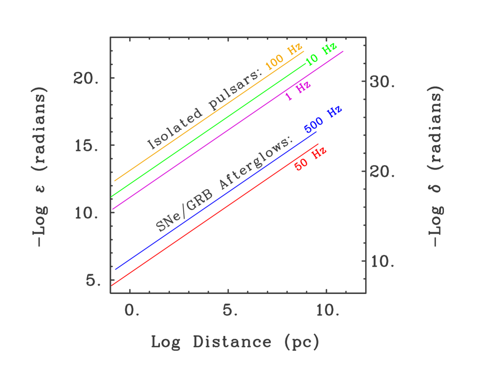
Figure 17: Left vertical scale: the -log of the angle, $\varepsilon$, from Fig. 3 as a function of the log distance (bottom horizontal scales), and the log of the angle, $\delta$ (right vertical scale), representing the upper limit for 1, 10, and 100 Hz isolated pulsars, and disruption of red (50 Hz) or blue (500 Hz) supergiants, whose cores have collapsed to neutron stars.

Assuming GRB afterglows are pulsars because of their long persistence and apparent 1/distance law, it is not unreasonable to think that scaling with $\varepsilon$ will hold to another factor of 10 in distance, from $\sim$55 kpc to the 778 kpc of M31 and the 898 kpc to M33, and that pulsars will be detected in these, even if the sampling in time is not fine enough to exploit any pulse narrowing (see three paragraphs below). Another conclusion which can be drawn from all this is that $\delta$ can be immeasurably small. Figure 17 shows the $\delta$ values for 1, 10, and 100 Hz isolated pulsars, and the red and blue supergiants which produce GRBs and afterglows from their supernovae.

From Fig. 17 and some work with a straightedge, we can see that the limiting pulse width ($\delta$) of a 1 Hz pulsar at $\sim$100 pc is $10^{-20}$ radians, or $\sim$1.6$\times 10^{-21}$ s. This rate is consistent with 1 ns after $\sim$4,900 km, and $\sim$20 ns at one characteristic distance for the decrease of $\varepsilon$ (232 km).

When the coherent range does reach $\phi_{limit}$, and then the distance increases by some factor, $\alpha$, decreasing $\varepsilon$ by the same factor, the range of phases which fall below the limiting $\phi^{3}/6$ curve falls by a factor of $\sqrt{\alpha}$. From our discussion near the end of Section III, we learned that the more limited source phase range has made the resulting pulse a factor of $\sim\sqrt{\alpha}$ narrower, which represents more energy by the same factor because of the increased bandwidth of the Fourier components of the narrower pulse, and sensible detection algorithms can exploit this. So even here, the effective distance law is still better than inverse square, while for less distant sources, every factor increase in distance causes that much more source within the same small time range, thus the 1/distance law applies.

An interesting possibility is the observation of Crab-like optical pulsars at great distances. Calculating $R_{\mathrm{LC}}\times(R-1/R)$ for a 25 Hz pulsar which produces a sharp pulse by pushing material through a typical observer inclination-determined $R$ of $2/\sqrt{3}=1.155$, or $60^{\circ}$ (30^∘ off the rotational plane), gives a scaling length for $\varepsilon$ of 551 km. It takes $5.6\times 10^{10}$ of these to make just one parsec. Thus $\varepsilon$ is $30^{\circ}/(5.6\times 10^{10})=9.3\times 10^{-12}$ radians, and $\delta=7\times 10^{-17}$ radians, or a whopping 1.3 $\mathrm{\AA}$ at $R_{\mathrm{LC}}$, or 4.3$\times 10^{-19}$ s. At this point, quantum effects may take over for all emission wavelengths longer than very soft X-rays, including the radio through the ultraviolet.

If a rotating, magnetized body can drag its magnetic field supraluminally across plasma, so can an orbiting, magnetized body, near a/the supermassive black hole in an AGN, and certainly any orbiting binary system. The focused radiation, which first moves in the Z direction (recall that $Z=\sqrt{R^{2}-1}\sqrt{X^{2}-1+1/R^{2}},~{}\mathrm{for}~{}X=\sqrt{1-1/R^{2}}~{}+$ ‘a small value,’ starts completely vertically) is ideal for forming jets perpendicular to the orbital plane/thin accretion disk. Such jets will not be nearly as highly collimated as pulsar-driven jets, but the observational constraints only demand 1 part in 100 collimation (and the occasional magnetic field line advected into the jet from material in the accretion disk).

Since magnetic field lines can not thread into uncharged black holes, they must somehow adjust when two of them are co-orbiting prior to merging, in a manner that ordinary matter can not mimic. Thus it is possible that this situation will also result magnetic fields moving supraluminally across matter, whose excitations may drive strong jets perpendicular to any surrounding, large accretion disks. This process may have caused the strong jets visible near M87 and within the Seyfert 2 galaxies in NGC 5128 (Centaurus A) and Cygnus A clusters, and Hercules A.

At the same time, an extragalactic black hole acquisition within M87, and Centaurus, Cygnus, and Hercules A, would also have taken any objects, which previously had been quietly orbiting either black hole, and scattered them to the four winds. There is also the systematic difference in the velocities of the nearby companion star populations left over from the merger of two host galaxies containing the black holes, as well as the kinetic energy deposited by either black hole due to dynamical friction. All of these effects would result in a mass estimate exaggerated by a factor of thousands. It is possible that all such estimates for black holes, in the billions of solar masses, have been the result of companion black hole acquisition. The strong linear relationM98 between host galaxy mass and the misattributed, virial black hole mass follows trivially.

Thus there is no longer any problem of the time needed to form such massive objects, simply because they are not that massive, at best in the few tens of millions of solar masses, easily possible to build from globular cluster black holes of a few million solar masses each. The recentaaa ; ddd “image” of the black hole in M87 is likely to be a large region between the two orbiting black holes ($\sim$336 au diameter for 20 $\mu$arc s in M87) that has been cleared of stars and luminous material by the periodic gravitational disturbance, rather than any event horizon large enough to be resolved.

VIII Other supraluminal excitations, GRBs and redshifts

Many, if not all, transient events in the distant Universe, including outbursts of AGNs and QSOs, on timescales of days-to-months, generally accepted as black-hole driven, to fast radio bursts, on timescales of milliseconds, are likely a result of one type of supraluminal excitation or another, and violate the inverse square law in certain directions, relieving the need for the extreme amounts of associated energy. Gamma-ray bursts, which last up to 100 seconds, may result from supernova core collapse and a linearly accelerated supraluminal excitation (the vCc’s on the path become increasingly open, intersecting with previous vCc’s, and generating focused beams in a ring around the direction of motion).

This occurs in a volume of circumstellar gas a dozen light-days distant ($d$), and is due to a beam collimated to about half a degree or so ($\delta\psi$), producing a delay range of $d(\delta\psi)^{2}/2\sim 50$ s.spot However, the afterglows of gamma-ray bursts, many of which can last for hours, could consist, at least partially, and at some time when there is plasma at the right radius, pulsar emission.M12

Since about half of all Swift gamma-ray bursts are known to have afterglows, then at least half of GRB progenitors leave pulsars behind, and at most half are black-hole-producing events. Of those events which produce pulsars, the ones due to core-merger supernovae could possibly be used to derive the redshift, as 500 Hz may be a standard candle in initial spin frequency for such objects, because there is always too much (orbital) angular momentum in the merger process, so the spin rate is set by the branching of the Maclaurin and Jacoby solutions.StirlingColgate

The optical signature of the neutron star-neutron star (NS-NS) merger in NGC 4993, GW170817, was still detectable four days after the event, though several magnitudes fainter, more likely indicating an outburst of some sort (see, e.g., [Fong17, ] and references therein). It may be possible that the rapid rotation involved in NS-NS mergers, along with a remnant magnetic field, produce supraluminal excitations which may drive much of the observed outburst phenomena. Gravitational supraluminal excitations of matter dense enough to, in turn, radiate strong focused gravitational waves, might be possible in NS-NS and even black hole-NS mergers.

IX General Discussion

IX.1 Pulsars

We have presented evidence that at lesat half of all Parkes radio pulsars have been discovered because we are close to a favored orientation (nearly perpendicular to the rotation axes) where their radiated power diminishes only as the first power of distance, and have calculated the onset of this effect in one instance, confirming a long-predicted effect.Ar94 ; AR04

Observationally, the effect holds for these pulsars at distances up to 10 kpc. Given the limited time resolution of almost all radio data, this can not be due to just the same energy concentrated into narrower and narrower pulses. Instead, out to some range of distances, more energy is concentrated into the same pulse width.

Interestingly, the strongest optical pulsations from SN 1987A, observed during 1993, 6 Feb.Opacity and 27 Aug. (at the 49.7 kpc distance to the LMC), amountedM00 ; M00c to a full 16% (magnitude 20.5) of the m_V=18.5 central star which persisted from about 1992-1995. Such pulsations correspond to an azimuth range of 60^∘ if this central source is entirely due to the pulsar, and more if only partly so. This implies, not coincidentally, that the pulsar was as bright as it could get during the two observations, lending further support to the pulsar model discussed in this work (but not for strongly-magnetized pulsars, such as the Crab).

IX.2 Supernovae

The effects of focused beams resulting from supraluminal excitations are still generally unappreciated by the scientific community. Accounting for these in the early stages of supernova disruption yields results that are highly anisotropic, but which are limited in collimation to 100 to 1 at best due to pulsar precession,M00 ; M00c and further limited because supraluminally induced polarization currents, though dominant, producing 0.62$\times$10⁵¹ ergs (0.62 foe) from a 500-467.5 Hz-spin-rate drop, is not the only disruption mechanism – there is also the production of ⁵⁶Ni, and its decay through positron emission to ⁵⁶Co.

In addition to the more obvious effects of anisotropy, we have from [M12, ] and considerations of this in Section VI.2, a considerable fraction of the maximum apparent luminosity of SNe is due to polar jets propagating through (and at the same time, bunching up) circumstellar/polar-ejected material. This material is about a light-week and a half distant, though closer, and possibly brighter, for C-O stars due to the high atomic numbers in the jets and target material. This (time varying) contribution to the apparent luminosity depends on, and is variably delayed due to, the orientation angle of the pulsar rotational axis.

It has also already been a decade and a half since critical observations were made of local SNe Ia which were clearly below the width-luminosity relation by nearly an order of magnitude,Benetti with none lying above it, and more than a dozen years since observers gave up on using them in that way.Siegfried Correcting just a few such objects in a distant sample could easily wipe out the -28% effect in luminosity, go on to overwhelm any reasonable correction for Malmquist bias (the last, best hope that less luminous distant SNe were due to a real effect), and still provide enough excess luminosity to imply a gravitationally-induced deceleration in the Universe for $\Omega_{M}~{}\sim~{}0.99$.

The reality might be worse, with many more SNe Ia lying under the Width-Luminosity relation by a lesser degree. In the end, this is a textbook example of systematic biases in the measurement, in this case, of supernova luminosity. The initial local sample of SNe Ia from [MMP, ] was determined by serendipity – only the very bright ones, detected one way or another, were available. Then the automated searches came online, and those in the distant sample were anomalously dim. It took almost another decade to augment the local sample, and some of these were drastically dimmer than would be expected on the basis of the width-luminosity relation.

Thus it is clear that were they not so luminous, SNe would be the last objects in the Universe anyone would want to use as standard candles. But they are that luminous, and fortunately, the very circumstellar material, that complicates their use as standard candles, may allow observation of many more relatively nearby SNe from before their instant of core collapse. “Bright Source 2” in SN 1987A was very likelyM18 due to material ejected from the poles some months prior to core collapse, and was bright enough to detect in progenitors out to a few Mpc, and so these can serve as predictors of core collapse.

A thorough study of a few relatively nearby SNe Ia just might lead to telltale details in these, that can also be measured in distant SNe, which can be used to determine the rotational orientation, as well as the physical properties of the circumstellar material and the kinematics of the jets. So, in the end, after some hard work, SNe Ia might actually be usable as standard candles.

But for now, the so-called “Standard Model of Cosmology,” with $\Omega_{\mathrm{M}}=0.04,~{}\Omega_{\mathrm{DM}}=0.24,$ $~{}\mathrm{and}~{}$ $\Omega_{\mathrm{DE}}=0.72$, has no particular advantage over any other dogma, given its discrediting by both observation (15 years ago) and now calculation, and should be avoided also because of the baggage of “dark energy” and “dark matter” that comes with it. Indeed, there is no firm evidence for either, other than effects due to non-viriality and/or viriality attributed to the wrong mass, for the latter. There is also the problem of early star formation for low fractions of $\Omega_{M}$, which can be alleviated in “bounce” models with high $\Omega_{M}$, along with the problems of light elements surviving the associated nucleosynthesis, and uniformity at the same time, without invoking “Inflation” (more baggage). The early formation of clusters, and their high kinetics, can be explained by pulsar-driven jets.M12

Still, students are being led down a primrose path of bad science (exploiting SNe for cosmologyJAK without first understandingdes them), ignorance (of the implications of SN 1987A as advanced in [M12, ] and [M09, ] years before), and prejudice (some favoring a radical cosmology with a fervor that would shame the most zealous religious fanatic), by, now, a second or third generation of mentors, in part, perhaps, due to the persistence of supporting grants, which should be replaced by others which are much more generic in nature.

Misunderstanding the nature of core-collapse SNe by everyone, particularly by those experts on the spectra and light curves of SNe, consulted to render judgement on an individual SN Ia which did not fit the “pattern” of anomalously dim Ia’s to disqualify an offending candidate, is not the best way to produce objective science. This may be the reason why the distribution of luminosities of qualified SNe Ia is not consistent with any known cosmology.RGV

The issue of thermonuclear SNe Ia was raised nearly a half century ago,Whelan and persists even today. However, Wolf-Rayet stars with merging cores massing 1.4 M_⨀ or more, as happened within Sk -69^∘202, will undergo core collapse and become SN Ia’s themselves, thereby ruining the sample, no matter if thermonuclear SN Ia’s, should they exist, can, by themselves, be used as standard candles.

IX.3 The Sun

Closer to home, it may be possible that the 5-minute oscillations in the SunHill also (sporadically) mimic a circularly supraluminal excitation. The circumference of the Sun is 14.7 light-sec, so supraluminal excitations are possible for any harmonic number above 20 in these p-waves, which, in an already-magnetized body, have an electromagnetic consequence. Harmonics exist well above 60, which would imply $R$ values at 3 or above. The more intermediate harmonics may put the initial focus close to, or just underneath the solar surface, possibly causing flares, and/or coronal mass ejections, and possibly evenSchaefer00 “superflares.” The highest harmonics can not dominate, or many of the flares and ejections would be polar. Whether the existence of such excitations will effect our estimates of $\textrm{T}_{\textrm{C}}$, its $\sim$15 million ^∘K core temperature, remains to be determined, (but if it does, the result may cast doubt on the existence of neutrino masses/flavor oscillations).

IX.4 Hercules X-1

Parts of the twisted, tilted, accretion disk around this 1.24 s X-ray pulsar will be illuminated by the pulsed, X-ray flux, thus producing supraluminal excitations, which may have resulted in very high energy pulsed radiation,D88 ; R88 ; L88 ; V89 observed in 1986, and upshifted in pulsed frequency by some 0.16%, three times the maximum gain of the pulsar from Doppler shift. Detailed discussion of this is too long to include here.

IX.5 Other effects

The mechanism of focused radiation may also be important to gamma-ray bursts and their afterglows, AGN jets, neutron star mergers, and most, if not all, other transient events in the distant Universe. But to actually calculate these things to the end of the Universe, a greater range of precision in computation (256 bits) will be necessary. Until that time, no calculation of supernovae, or any other large object involving supraluminal excitations and their resulting focused beams will be possible. A few more orders of magnitude may be achieved for the supernova problem by iterating to find the minimum slope of the observer time as an indicator, rather than fine-raster source times and histogramming the resulting observer times as plotted in Fig. 11, though this latter is visually more dramatic.

The search for effects of physics “Beyond the Standard Model” continues, but it is clear that the effects of supraluminal excitations are: real (but were never considered until very recently), responsible for many effects in the distant Universe, and should themselves be considered as additions to the Standard Model of Physics.

X Conclusion

Focused beams, produced by supraluminally undpated polarization currents driven by the neutron star/pulsar remnant, are the dominant disruption mechanism for most, if not all supernovae (about a decade down the road, this back-to-back, dual particle accelerator runs through all of the stellar material). Nearly all progenitor stars are large enough so that the beam emergences cluster around the rotational poles, producing polar jets.

The jets will crash into material ejected previously by the same mechanism, acting through the increasing stellar core rotation rate, producing a significant contribution to the total SN luminosity which varies strongly with rotational orientation. The timing of this contribution also varies by several days, again according to the rotational orientation to the observer. They will not be useful as standard candles anytime soon, but there is some hope that SNe can be understood in sufficient detailM18 to change this. Until then, they provide no constraint on cosmological constants.

Because the mechanism discussed here dominates the disruption of SNe, all previous calculations which successfully disrupted progenitors without accounting for it are now embarrassingly incorrect, and will have to be modified to accommodate this new understanding of reality.

In addition, nearly all solitary progenitor stars spend their lives burning to heavier and heavier elements in their cores, and in consequence the moments of inertia of their magnetized cores will also fall and their rotation will speed up during their lifespans. Thus the same mechanism, that later disrupts SN progenitors, will cause material ejection in all sufficiently large stars before core collapse (if that happens). It will also disrupt would-be “Direct Collapse” stars long before they achieve masses anywhere close to a billion solar.

Since there is no way to produce billion-solar-mass black holes in the lifetime of the Universe, galaxies with jets and black holes thought to weigh in the billions of solar, such as M87, and Centaurus, Cygnus, and Hercules A, are likely the result of binary, few-million solar mass black holes, the result of mergers and capture by dynamical friction (else, where are the few-million-solar-mass black hole binaries, and how would they appear?).

AGN jets likely do not originate directly from their black holes, but rather from supraluminal excitations in the surrounding disk material, in turn produced by magnetic fields moving supraluminally due to orbiting magnetic bodies, and/or time varying gravitational fields from (most likely two) orbiting, black holes with masses in the millions of solar.

In order to calculate these effects well to the ends of the Universe, computers will have to be much more precise, possibly using as many as 256 bits for its constants and variables.

- (1) Houshang Ardavan, “The Mechanism of Radiation in Pulsars,” MNRAS 268 (2), 361–392 (1994).
- (2) Houshang Ardavan, “Generation of focused, non-spherically decaying pulses of electromagnetic radiation,” Phys. Rev. 58 (5), 6659–6684 (1998).
- (3) Houshang Ardavan, Arzhang Ardavan, & John Singleton, “Frequency spectrum of focused broadband pulses of electromagnetic radiation generated by polarization currents with superluminally rotating distribution patterns,”JOSAA 20 (11), 2137–2155 (2003).
- (4) Houshang Ardavan, Arzhang Ardavan, & John Singleton, “Spectral and polarization characteristics of the nonspherically decaying radiation generated by polarization currents with superluminally rotating distribution patterns,” JOSAA 21 (5), 858–872 (2004).
- (5) Houshang Ardavan, Arzhang Ardavan, & John Singleton, “Morphology of the nonspherically decaying radiation beam generated by a rotating superluminal source,” JOSAA 24 (8), 2443–2458 (2007).
- (6) Houshang Ardavan, Arzhang Ardavan, John Singleton, Joseph Fasel, & Andrea Schmidt, “Spectral properties of the nonspherically decaying radiation generated by a rotating superluminal source,” JOSAA 25 (3), 780–784 (2008).
- (7) Houshang Ardavan, Arzhang Ardavan, John Singleton, & Mario R. Perez, “Mechanism of generation of the emission bands in the dynamic spectrum of the Crab pulsar,” MNRAS 388 (2), 873–883 (2008).
- (8) T. H. Hankins, & J. A. Eilek, “Radio Emission Signatures in the Crab Pulsar,” ApJ 670 (1), 693–701 (2007).
- (9) Houshang Ardavan, Arzhang Ardavan, John Singleton, Joseph Fasel, William Junor, John Middleditch, Mario R. Perez, Andrea Schmidt, Pinaki Sengupta, & Petr Volegov, “Comparison of multiwavelength observations of 9 broad-band pulsars with the spectrum of the emission from an extended current with a superluminally rotating distribution pattern,” arXiv:0908.1349 (2009).
- (10) There are actually two very closely spaced peaks, which are almost never resolved. However, the peak of the 62 Hz pulsar, J0537-6910, may in fact be resolved into two peaks when treated with sufficient care (see 2006ApJ…652.1531M)
- (11) John Middleditch, “Pulsar-Driven Jets in Supernovae, Gamma-Ray Bursts, and the Universe,” Ad. Ast. id. 898907, 26pp, <http://www.hindawi.com/journals/aa/2012/898907> (2012).
- (12) With the exception of young, strongly magnetized pulsars such as the Crab, which can drive strong plasma winds within which other features of the pulse profile can be generated (see near the end of Section VI).
- (13) Andrea Caroline Schmidt-Zweifel, “Terrestrial and Extraterrestrial Radiation Sources that Move Faster than Light,” Master’s Thesis, University of New Mexico, Mathematics, <http://digitalrepository.unm.edu/math_etds/45/> (2012).
- (14) R. N. Manchester, G. B. Hobbs, A. Teoh, & M. Hobbs, AJ 129, 1993–2006 (2005). <http://www.atnf.csiro.au/research/pulsar/psrcat/> (2016).
- (15) Shantanu Desai, “Do Pulsar Radio Fluxes violate the Inverse-Square Law,” Ap. & SS 361, id. 138, (2016).
- (16) G. Estathiou, Richard S. Ellis, & Bruce A. Peterson, “Analysis of a complete galaxy redshift Survey. II — The Field- galaxy luminosity function,” MNRAS 232, 431–461 (1988).
- (17) The 1.1 ms FWHM of the Crab Pulsar main pulse (not included in the Parkes sample) is close to 3% of its 33 ms period, so 3% is the selector value which first came to mind, and it immediately succeeded in splitting the sample in half.
- (18) John Singleton, Pinaki Sengupta, John Middleditch, Todd L. Graves, Mario Perez, Houshang Ardavan, & Arzhang Ardavan, “A Maximum-Likelihood Analysis of Observational Data on Fluxes and Distances of Radio Pulsars: Evidence for Violation of the Inverse-Square Law,” arXiv:0912.0350 (2009).
- (19) James W. Cordes, & T. Joseph W. Lazio, “NE2001.I. A New Model for the Galactic Distribution of Free Electrons and its Fluctuations,” arXiv:astro-ph/0207156 (2002).
- (20) James W. Cordes, & T. Joseph W. Lazio, “NE2001. II. Using Radio Propagation Data to Construct a Model for the Galactic Distribution of Free Electrons,” arXiv:astro-ph/0301598 (2003).
- (21) Eduardo B. Amôres, & Jacques R. D. Lépine, “Models for interstellar extinction in the Galaxy,” AJ, 130, 659–673 (2005).
- (22) G. M. Lilley, R. Westly, A. H. Yates, & J. R. Busing, “The Supersonic Bang,” Nature 171 id. 4362, 994–996 (1953).
- (23) Ioannis Contopoulos, Constantinos Kalapotharakos, & Demosthenes Kazanas, “A New Standard Pulsar Magnetosphere,” ApJ 781 (1), 46–50 (2014).
- (24) John Middleditch, Carleton R. Pennypacker, & M. Shane Burns, “Optical color, polarimetric, and timing measurements of the 50 MS Large Magellanic Cloud pulsar, PSR 0540-69,” ApJ 315, 142–148
- (25) Martin C. Weisskopf, J. Jeff Hester, A. Tennant, Ronald F. Elsner, Norbert S. Schulz, Herman L. Marshall, Margarita Karovska, Joy S. Nichols, Douglas A. Swartz, Jeffery J. Kolodziejczak, & Stephen L. O’Dell, “Discovery of Spatial and Spectral Structure in the X-ray Emission from the Crab Nebula,” Apj 536 (2), L81–L84 (2000).
- (26) Michael F. Bietenholz, & Norbert Bartel, “SN 1986J VLBI. IV. The Nature of the Central Component,” ApJ 851 (1), article id 7, 12 pp (2017).
- (27) Gain Luca Israel, Andrea Belfiore, Paolo Esposito, Pier Giorgio Casella, Andrea De Luca, Martino Marelli, Alessandro Papitto, Matteo Perri, Simonetta Puccetti, Guillermo A. Rodríguez Castillo, David Salvetti, Andrea Tiengo, Luca Zampieri, Daniele D’Agostino, Jochen Greiner, Frank Haberl, Giovanni Novara, Ruben Salvaterra, Roberto Turolla, Mike Watson, Joern Wilms, & Anna Wolt, “An accreting pulsar with extreme properties drives an ultraluminous x-ray source in NGC 5907,” Sci 355 id. 6327, 817–819 (2017).
- (28) Unfortunately, both locations of this project will be in the Southern Hemisphere, whereas the two spirals in the Local Group, other than our own Milky Way, M31 and M33, are solidly in the northern sky at and , see <http://www.skatelescope.org/location>.
- (29) E. Rubio-Herrera, B. W. Stappers, J. W. T. Hessels, & R. Braun, “A search for radio pulsars and fast transients using the Westerbork Synthesis Radio Telescope,” MNRAS 428, 2857–2873 (2013).
- (30) Interstellar scattering throws energy from this pulse into the neighboring 50 ms, which averages 20% as high — if this was not included in the PKSMB S1400 flux estimate, then it would be closer to the most luminous.
- (31) Five-hundred-meter Aperture Spherical radio Telescope, <http://fast.bao.ac.cn/en>.
- (32) At 1400 MHz – if the spectrum of B1302 is steeper than most, then it will move up a bit in the order at the Westerbork 328 MHz frequency.
- (33) However, narrower peaks in Fourier space are also easier to detect using any reasonably sophisticated search methods.
- (34) N. I. Serafimovich, Yu. A. Shibanov, P. Lundqvist, & J. Sollerman, “The young pulsar PSR B0540-69.3 and its synchrotron nebula in the optical and X-rays,” AA 425, 1041–1060 (2004).
- (35) The Chandra Team, “Chandra :: Photo Album,” <http://chandra.harvard.edu/photo/2004/snr0540> (2016).
- (36) J. Middleditch, F. E. Marshall, Q. D. Wang, E. Gotthelf, & W. Zhang, “Predicting the Starquakes in PSR J0537-6910,” ApJ 652 (1), 1531–1546 (2006).
- (37) John Middleditch, Jerome A. Kristian, William E. Kunkel, Kym M. Hill, Robert D. Watson, Richard Lucinio, James N. Imamura, Thomas Y. Steiman-Cameron, Andrew Shearer, Raymond Butler, Michael Redfern, & Anthony C. Danks, “Rapid Photometry of supernova 1987A: a 2.14 ms pulsar?” NewA 5 (5), 243–283 (2000).
- (38) John Middleditch, Jerome A. Kristian, William E. Kunkel, Kym M. Hill, Robert D. Watson, Richard Lucinio, James N. Imamura, Thomas Y. Steiman-Cameron, Scott M. Ransom, Andrew Shearer, Raymond Butler, Michael Redfern, & Anthony C. Danks, “A 2.14 ms Candidate Optical Pulsar in SN 1987A,” ArXiv:astro-ph0010044 (2000).
- (39) Peter Nisenson, & Costas Papaliolios, “A second bright source detected near SN 1987A,” ApJ, 518 (1), L29–L32 (1999).
- (40) Peter Nisenson, Costas Papaliolios, Marguerite Karovska, & Robert Noyes, “Detection of a very bright source close to the LMC supernova SN 1987A,” ApJ 320 (2), L15–L18 (1987).
- (41) W. P. S. Meikle, S. J. Matcher, & B. L. Morgan, “Speckle interferometric observations of supernova 1987A and of a bright associated source,” Nature 329 (6140), 608–607 (1987).
- (42) Lifan Wang, J. Craig Wheeler, Peter Hoflich, Alexi Khoklov, Dietrich Baade, David Branch, Peter Challis, Alexei V. Filippenko, Claes Fransson, Peter Garnavich, Robert P. Kirshner, Peter Lundqvist, Richard McCray, Nino Panagia, Chun S. J. Pun, Mark. M. Phillips, George Sonneborn, & Nicholas B. Suntzeff, “The Axisymmetric Ejecta of Supernova 1987A,” ApJ 579 (1), 671–677 (2002).
- (43) John Middleditch, “Predicting the next local supernova,” arXiv:1910.03797 (2019).
- (44) One reviewer denied that a rotating central, obliquely magnetized core (or pair of merging cores) would eject matter from a sufficiently large star, all the while accepting other effects resulting from situations with exactly the same mathematics. It’s easy to sit in one’s local pub, swigging a pint of one’s favorite brew, and claim that just by viewing the situation in one’s “mind’s eye,” without ever having drawn Huygen’s wavelets from any example of an accelerating supraluminal excitation, and claim that such a star will not throw off matter. However, if Sk-69o202 were plotted on an 8.5 by 11-inch sheet of paper, the speed of light would be about one mm per second, and that matters. The old-timer’s at Lick Observatory had a more informed opinion: “They do that.” – Gene Harlan, 1970’s.
- (45) Mario Hamuy, & Nicholas B. Suntzeff, “SN 1987A in the LMC. III - UBVRI photometry at Cerro Tololo,” AJ 99, 1146–1158 (1990).
- (46) Daniel Kasen, Peter Nugent, Lifan Wang, D. A. Howell, Craig Wheeler, Peter Hoflich, Dietrich Baade, E. Baron, and P. H. Hauschildt, “Analysis of the Flux and Polarization Spectra of the Type Ia Supernova SN 2001el: Exploring the Geometry of the High-Velocity Ejecta,” ApJ 593 (2), 788–808 (2003).
- (47) John Magorrian, Scott Tremaine, Douglas Richstone, Ralf Bender, Gary Bower, Alan Dressler, S. M. Faber, Karl Gebhardt, RIchard Green, Carl Grillmair, John Kormendy, & Tod Lauer, “The Demography of Massive Dark Objects in Galaxy Centers,” AJ 114 (6), 2285 – 2305 (1998).
- (48) The EHT collaboration, “First M87 Event Horizon Telescope Results. I. The Shadow of the Supermassive Black Hole,” ApJ, 875 (1), L1 (2019).
- (49) The EHT collaboration, “First M87 Event Horizon Telescope Results. IV. Imaging the Central Supermassive Black Hole,” ApJ, 875 (1), L4 (2019).
- (50) But continued beam and particle input, over days and weeks, sweeps up and heats material, producing, eventually, a spot with 8% of the H light from the supernova!Nis ; MMM
- (51) Stirling A. Colgate, private communication, (1992).
- (52) W. Fong, E. Berger, P. K. Blanchard, R. Margutti, P. S. Cowperthwaite, R. Chornock, K. D. Alexander, B. D. Metzger, V. A. Villar, M. Nicholl, T. Eftekhari, P. K. G. Williams, J. Annis, D. Brout, D. A. Brown, H.-Y. Chen, Z. Doctor, H. T. Diehl, D. E. Holz, A. Rest, M. Sako, & M. Soares-Santos, “The Electromagnetic Counterpart of the Binary Neutron Star Merger LIGO/Virgo GW170817. VIII. A Comparison to Cosmological Short-duration Gamma-Ray Bursts” ApJ 848 (2), L23–L31 (2017).
- (53) The observations during 1993, Feb.,M00 ; M00c suffered an extra factor of two extinction due to a volcanic eruption in the south of Chile about a month prior.
- (54) Stefano Benetti, Enrico Cappellaro, Paolo Mazzali, M. Turatto, Giuzeppi Altavilla, F. Bufano, N. Elias-Rosa, Rubina Kotak, Giuliano Pignata, Maria Elena Salvo, Vallery Stanishev, “The Diversity of Type Ia Supernovae: Evidence for Systematics?,” ApJ 623 (2), 1011–1016, (2005).
- (55) Tom Siegfried, “Surveys of exploding stars show one size does not fit all,” Science 316 (5822), 194–195 (2007).
- (56) Mark M. Phillips, “The Absolute Magnitudes of Type IA Supernovae,” ApJ 413 (1), L105–L108 (1993).
- (57) Jerome A. Kristian, private communication (November 1994).
- (58) The instigation of this process may have been driven, in part, by increasing desperation in a “now or never” sense, at a time when SN 1987A was producing more questions than answers.
- (59) John Middleditch, “Pulsed Gamma-Ray Burst Afterglows,” <http://arxiv.org/abs/0909.2604>, (2009).
- (60) Ram Gopal Vishwakarma, “Do Recent Supernovae Ia Observations Tend to Rule Out all the Cosmologies?” IJMPD 16 (10), 1641–1651 (2007).
- (61) John Whelan, & Icko Iben, Jr., “Binaries and Supernovae of Type I,” ApJ 186, 1007–1014 (1973).
- (62) Frank Hill, “Solar Oscillations” in Allen’s Astrophysical Quantities Section 14.3, 342-347 (2000) AIP Press, Springer-Verlag, New York, Berlin, Heidelberg, Arthur N. Cox, Editor, ISBN 0-387-98746-0.
- (63) Bradley E. Schaefer, Jeremy R. King, & Constantine P. Deliyannis, “Superflares on Ordinary Solar-Type Stars,” ApJ 529 (2), 1026–1030 (2000).
- (64) B. L. Dingus, D. E. Alexandreas, R. C. Allen, R. L. Burman, K. B. Butterfield, R. Cady, C. Y. Chang, R. W. Ellsworth, J. A. Goodman, S. K. Gupta, T. J. Haines, D. A. Krakauer, J. Lloyd-Evans, D. E. Nagle, M. Potter, V. D. Sandberg, R. L. Talaga, & C.A. Wilkinson, “Ultrahigh-energy pulsed emission from Hercules X-1 with anomalous air-shower muon production,” PRL 61 (17), 1906–1909 (1988).
- (65) L. K. Resvanis, A. Szentgyorgyi, J. Hudson, L. Kelley, J. G. Learned, C. Sinnis, V. Stenger, D. D. Weeks, J. Gaidos, M. Kertzman, F. Loeffler, T. Palfrey, G. Sembroski, C. Wilson, U. Camerini, J. P. Finley, W. Fry, J. Jennings, A. Kenter, M. Lomperski, R. Loveless, R. March, J. Matthews, R. Morse, D. Reeder, & P. Slane, “VHE gamma rays from Hercules X-1,” ApJ 328 (2), L9–L12 (1988).
- (66) R. C. Lamb, M. F. Cawley, D. J. Fegan, K. G. Gibbs, P. W. Gorham, A. M. Hillas, D. A. Lewis, N. A. Porter, P. T. Reynolds, & T. C. Weekes, “TeV gamma rays from Hercules X-l pulsed at an anomalous frequency,” ApJ 328 (2), L13–L16 (1988).
- (67) P. R. Vishwanath, P. N. Bhat, P. V. Ramanamurthy, & B. V. Sreekantan, “A possible very high energy gamma-ray burst from Hercules X-1,” ApJ 342 (1), 489–492 (1989).