Greedy Convex Ensemble

Abstract

We consider learning a convex combination of basis models, and present some new theoretical and empirical results that demonstrate the effectiveness of a greedy approach. Theoretically, we first consider whether we can use linear, instead of convex, combinations, and obtain generalization results similar to existing ones for learning from a convex hull. We obtain a negative result that even the linear hull of very simple basis functions can have unbounded capacity, and is thus prone to overfitting; on the other hand, convex hulls are still rich but have bounded capacities. Secondly, we obtain a generalization bound for a general class of Lipschitz loss functions. Empirically, we first discuss how a convex combination can be greedily learned with early stopping, and how a convex combination can be non-greedily learned when the number of basis models is known a priori. Our experiments suggest that the greedy scheme is competitive with or better than several baselines, including boosting and random forests. The greedy algorithm requires little effort in hyper-parameter tuning, and also seems able to adapt to the underlying complexity of the problem. Our code is available at https://github.com/tan1889/gce.

1 Introduction

Various machine learning methods combine given basis models to form richer models that can represent more complex input-output relationships. These include random forests (Breiman, 2001) and boosting (Freund and Schapire, 1995; Mason et al., 2000a; Chen and Guestrin, 2016), which have often been found to work well in domains with good features. Interestingly, even combining simple basis models like decision stumps can work very well on hard problems (Viola and Jones, 2004).

In this paper, we consider learning an optimal convex combination of basis models (Lee et al., 1996; Mannor et al., 2003; Oglic and Gärtner, 2016; Wyner et al., 2017), and present new theoretical and empirical insights.

We first compare learning from convex hulls with learning from the closely related linear hulls. Learning from a convex hull can be seen as a regularized version of learning from the corresponding linear hull, where we enforce constraints on the weights of the basis functions. While linear hulls are known to provide universal approximations (Barron, 1993; Makovoz, 1996), our analysis shows that they can be prone to overfitting. Specifically, we show that the capacity of the linear hull of very simple functions can be unbounded, while the convex hull is still rich but has bounded capacity.

Our second contribution is a generalization result for a general class of Lipschitz loss functions. A number of works studied algorithms for learning a convex combination and analyzed their generalization performance. However, previous works mostly focused on generalization performance with quadratic loss (Lee et al., 1996; Mannor et al., 2003) or large margin type analysis (Koltchinskii and Panchenko, 2005) for classification problems. The quadratic loss is a special case of the class of Lipschitz loss functions considered in this paper. In addition, our result shows that we can obtain an $O(1/\sqrt{n})$ convergence rate for log-loss in the classification setting.

Empirically, we present an extensive experimental evaluation of algorithms for learning from convex hulls. While previous works mainly focused on simple greedy algorithms to learn a convex combination, we leverage on the functional optimization versions of some sophisticated algorithms to develop algorithms for learning a convex combination. In particular, we consider the Frank-Wolfe (FW) algorithm and its variants (Jaggi, 2013), which provide natural ways to build convex combinations. We also show how a convex combination can be non-greedily learned when the number of basis functions is known a priori. Our experiments suggest that the greedy scheme is competitive with or better than several baselines, including boosting and random forests. The greedy algorithm requires little hyper-parameter tuning, and also seems to adapt to the underlying complexity of the problem.

Section 2 further discusses related works. Section 3 presents our theoretical analysis for learning from a convex hull. Section 4 discusses some greedy learning algorithms, and a non-greedy version. Section 5 empirically compares the algorithms for learning from convex hulls, and a few baselines. Section 6 concludes the paper.

2 Related Work

A number of works have studied the generalization performance of algorithms for learning convex combinations. Lee et al. (1996) considered learning a convex combination of linear threshold units with bounded fan-in (#inputs) for binary classification using quadratic loss, and they showed that an optimal convex combination is PAC-learnable. Mannor et al. (2003) also considered binary classification, and obtained a generalization result for general basis functions and quadratic loss. They also obtained a consistency result for more general loss functions. Koltchinskii and Panchenko (2005) provided some generalization results for learning a convex combination by maximizing margin. Oglic and Gärtner (2016) considered regression with quadratic loss and presented a generalization analysis for learning a convex combination of cosine ridge functions. We obtained generalization bounds for a class of Lipschitz loss functions and general basis functions.

Various authors considered greedy approaches for learning a convex combination, which iteratively constructs a convex combination by choosing a good convex combination of the previous convex combination and a new basis function. Jones (1992) presented a greedy algorithm and showed that it converges at $O(1/k)$ rate for quadratic loss. This is further developed by Lee et al. (1996) and Mannor et al. (2003). Zhang (2003) generalized these works to convex functionals. We leverage on the functional versions of more sophisticated greedy optimization algorithms; in particular, the FW algorithm and its variants, which have recently attracted significant attention in the numerical optimization literature (Jaggi, 2013). Recently, Bach (2017) considered using the FW algorithm to learn neural networks with non-Euclidean regularizations, and showed that the sub-problems can be NP-hard. Besides greedy approaches, we show how to non-greedily learn a convex combination given the number of basis functions. We empirically compared the effectiveness of these algorithms.

Works on random forests (Breiman, 2001) and boosting (Mason et al., 2000b) are also closely related. A random forest can be viewed as a convex combination of trees independently trained on bootstrap samples, where the trees have equal weights. Boosting algorithms greedily construct a conic, instead of convex, combination of basis functions, but for binary classification, a conic combination can be converted to a convex combination without changing the predictions. There are numerous related works on the generalization performance of boosting (e.g. see (Bartlett and Traskin, 2007; Schapire, 2013; Gao and Zhou, 2013)). Random forests are still less well understood theoretically yet (Wyner et al., 2017), and analysis can require unnatural assumptions (Wager and Walther, 2015). We empirically compared algorithms for learning a convex combination with random forests and boosting.

There have been also several recent applications of boosting for generative models. Specifically, Locatello et al. (2018) show that boosting variational inference satisfies a relaxed smoothness assumption which is sufficient for the convergence of the functional Frank-Wolfe algorithm; Grover and Ermon (2018) consider Bayes optimal classification; and Tolstikhin et al. (2017) propose AdaGAN, which is adapted from AdaBoost for Generative Adversarial Networks. Our work is orthogonal to these works in the sense that we study discriminative models and learning from a convex hull, instead of a linear or a conic hull. Moreover, our bound might be interesting in comparison to vacuous bounds that grow rapidly in the number of parameters: while the number of parameters for a convex combination can be unbounded, our error bound depends only on the pseudodimension of the basis models.

3 Theoretical Analysis

Given an i.i.d. sample ${\mathbf{z}}=((x_{1},y_{1}),\ldots,(x_{n},y_{n}))$ drawn from a distribution $P(X,Y)$ defined on ${\mathcal{X}}\times{\mathcal{Y}}\subseteq{\mathcal{X}}\times{\mathbf{R}}$, we want to learn a function $f$ to minimize the risk $R(f)={\mathbb{E}}L(Y,f(X))$, where $L(y,\hat{y})$ is the loss that $f$ incurs when predicting $y$ as $\hat{y}$, and the expectation is taken wrt $P$. The empirical risk of $f$ is $R_{n}(f)={\mathbb{E}}_{n}L(Y,f(X))=\frac{1}{n}\sum_{i=1}^{n}L(y_{i},f(x_{i}))$. Without loss of generality, we assume ${\mathcal{X}}\subseteq{\mathbf{R}}^{d}$.

Given a class of basis functions ${\mathcal{G}}\subseteq{\mathcal{Y}}^{{\mathcal{X}}}$, we use $\operatorname{co}_{k}({\mathcal{G}})$ to denote the set of convex combinations of $k$ functions in ${\mathcal{G}}$, that is, $\operatorname{co}_{k}({\mathcal{G}})=\{\sum_{i=1}^{k}\alpha_{i}g_{i}:\sum_{i}\alpha_{i}=1,\text{each }\alpha_{i}\geq 0,\text{each }g_{i}\in{\mathcal{G}}\}$. The convex hull of ${\mathcal{G}}$ is $\operatorname{co}({\mathcal{G}})=\cup_{k\geq 1}\operatorname{co}_{k}({\mathcal{G}})$. We will also use $\operatorname{lin}_{k}({\mathcal{G}})$ to denote the set of linear combinations of $k$ functions in ${\mathcal{G}}$, that is, $\operatorname{lin}_{k}({\mathcal{G}})=\{\sum_{i=1}^{k}\alpha_{i}g_{i}:\alpha_{1},\ldots,\alpha_{k}\in{\mathbf{R}},g_{1},\ldots,g_{k}\in{\mathcal{G}}\}$. The linear hull of ${\mathcal{G}}$ is $\operatorname{lin}({\mathcal{G}})=\cup_{k\geq 1}\operatorname{lin}_{k}({\mathcal{G}})$. The basis functions are assumed to be bounded, with ${\mathcal{G}}\subseteq{\mathcal{Y}}^{{\mathcal{X}}}\subseteq[-B,B]^{{\mathcal{X}}}$ for some constant $B>0$.

Capacity measures. A function class needs to be rich to be able to fit observed data, but cannot be too rich so as to make generalization possible, that is, it needs to have the right capacity. Commonly used capacity measures include VC-dimension, pseudodimension, and Rademacher complexity.

VC-dimension is defined for binary valued functions. Specifically, for a class ${\mathcal{F}}$ of binary valued functions, its VC-dimension $d_{VC}({\mathcal{F}})$ is the largest $m$ such that there exists $m$ examples $x_{1},\ldots,x_{m}$ such that the restriction of ${\mathcal{F}}$ to these examples contains $2^{m}$ functions. Equivalently, for any $y_{1},\ldots,y_{m}\in\{0,1\}$, there is a function $f\in{\mathcal{F}}$ such that $f(x_{i})=y_{i}$ for all $i$. $x_{1},\ldots,x_{m}$ is said to be shattered by ${\mathcal{F}}$.

Pseudodimension (Pollard, 1984) is a generalization of VC-dimension to real-valued functions. The pseudodimension $d_{P}({\mathcal{F}})$ of a class of real-valued functions ${\mathcal{F}}$ is defined as the maximum number $m$ such that there exists $m$ inputs $x_{1},\ldots,x_{m}\in{\mathcal{X}}$, and thresholds $t_{1},\ldots,t_{m}\in{\mathbf{R}}$ satisfying $\{({\mathbb{I}}(f(x_{1})\geq t_{1}),\ldots,{\mathbb{I}}(f(x_{m})\geq t_{m})):f\in{\mathcal{F}}\}=\{0,1\}^{m}$. If each $f\in{\mathcal{F}}$ is binary-valued, then $d_{P}({\mathcal{F}})=d_{VC}({\mathcal{F}})$.

Rademacher complexity is defined as ${\mathbb{E}}\sup_{f\in{\mathcal{F}}}{\mathbb{R}}_{n}f$, where ${\mathbb{R}}_{n}$ is the Rademacher process defined by ${\mathbb{R}}_{n}f=\frac{1}{n}\sum_{i}\epsilon_{i}f(x_{i},y_{i})$, with $(x_{i},y_{i})$’s being an i.i.d. sample, and $\epsilon_{i}$’s being independent Rademacher random variables (i.e., they have probability 0.5 to be -1 and 1). Expectation is taken wrt both the random sample and the Rademacher variables.

We refer the readers to the book of Anthony and Bartlett (2009) and the article of Mendelson (2003) for excellent discussions on these capacity measures and their applications in generalization results.

3.1 A Regularization Perspective

Several authors showed that linear hulls of various basis functions are universal approximators (Barron, 1993; Makovoz, 1996). Naturally, one would like to learn using linear hulls if possible. On the other hand, the richness of the linear hulls also imply that they may be prone to overfitting, and it may be beneficial to consider regularization.

Learning from the convex hull can be seen as a regularized version of learning from the linear hull, where the regularizer is ${\mathbb{I}}_{\infty}(f)=\begin{cases}0,&f\in\operatorname{co}({\mathcal{G}}),\\ \infty,&\text{otherwise}.\end{cases}$. This is similar to $\ell_{2}$ regularization in the sense that $\ell_{2}$ regularization constrained the weights to be inside an $\ell_{2}$ ball, while here we constrain the weights of the basis model to be inside a simplex. A key difference is that standard $\ell_{2}$ regularization is often applied to a parametric model with fixed number of parameters, but here the number of parameters can be infinite.

We compare the capacities of the linear hull and the convex hull of a class of basis functions ${\mathcal{G}}$ with finite pseudodimension, and demonstrate the effect of the regularizer ${\mathbb{I}}_{\infty}$ in controlling the capacity: while the convex hull can still be rich, it has a more adequate capacity for generalization.

For a class of functions ${\mathcal{F}}$, we shall use $\operatorname{bin}({\mathcal{F}})=\{x\mapsto{\mathbb{I}}(f(x)\geq t):f\in{\mathcal{F}},t\in{\mathbf{R}}\}$ to denote the thresholded binary version of ${\mathcal{F}}$. Consider the set of linear threshold functions ${\mathcal{T}}=\{{\mathbb{I}}(\theta^{\top}x\geq t):\theta\in{\mathbf{R}}^{d},t\in{\mathbf{R}}\}$. It is well-known that the VC-dimension of the thresholded versions of the linear combination of $k$ linear threshold functions can grow quickly.

Proposition 1.

((Anthony and Bartlett, 2009), Theorem 6.4) The VC-dimension of $\operatorname{bin}(\operatorname{lin}_{k}({\mathcal{T}}))$ is at least $\frac{dk}{8}\log_{2}\left(\frac{k}{4}\right)$ for $d>3$ and $k\leq 2^{d/2-2}$.

The above result implies that $d_{P}(\operatorname{lin}_{k}({\mathcal{T}}))$ is at least $\frac{dk}{8}\log_{2}\left(\frac{k}{4}\right)$. A natural question is whether the VC-dimension still grows linearly when $k>2^{d/2-2}$. We give an affirmative answer via a constructive proof, and provide counterpart results for the convex hull.

Proposition 2.

(a) Assume that $d\geq 2$. Then $d_{VC}(\operatorname{bin}(\operatorname{lin}_{k}({\mathcal{T}})))\geq k$, thus $d_{P}(\operatorname{lin}_{k}({\mathcal{T}}))\geq k$, and $d_{P}(\operatorname{lin}({\mathcal{T}}))=\infty$. In addition, the Rademacher complexity of $\operatorname{lin}({\mathcal{T}})$ is infinite.
(b) Assume that $d\geq 2$. Then $d_{VC}(\operatorname{bin}(\operatorname{co}_{k+1}({\mathcal{T}})))\geq k$, thus $d_{P}(\operatorname{co}_{k+1}({\mathcal{T}}))\geq k$, and $d_{P}(\operatorname{co}({\mathcal{T}}))=\infty$, but the Rademacher complexity of $\operatorname{co}({\mathcal{T}})$ is finite.

Proof.

(a) Consider an arbitrary unit circle centered at the origin, and any $k$ points $x_{1},\ldots,x_{k}$ which are equally spaced on the circle. Let $\theta_{i}=x_{i}$ and $b_{i}=1$ for $i=1,\ldots,k$. For any $y_{1},\ldots,y_{k}\in\{0,1\}$, consider the linear combination $f(x)=\sum_{i=1}^{k}w_{i}{\mathbb{I}}(\theta_{i}^{\top}x\geq b_{i})$, with $w_{i}=y_{i}$. We have $f(x_{i})=y_{i}$. The classifier $t(x)={\mathbb{I}}(f(x_{i})\geq 1)$ is a thresholded classifier obtained from $f$, and thus $t\in\operatorname{bin}(\operatorname{lin}_{k}({\mathcal{T}}))$. In addition, $t(x)={\mathbb{I}}(y_{i}\geq 1)=y_{i}$. In short, for any $y_{1},\ldots,y_{k}\in\{0,1\}$, there is a classifier $t\in\operatorname{bin}(\operatorname{lin}_{k}({\mathcal{T}}))$ such that $t(x_{i})=y_{i}$. Thus $d_{VC}(\operatorname{bin}(\operatorname{lin}_{k}({\mathcal{T}})))\geq k$. It follows that $d_{P}(\operatorname{lin}_{k}({\mathcal{T}}))\geq k$, and thus $d_{P}(\operatorname{lin}({\mathcal{T}}))=\infty$.

The Rademacher complexity of $\operatorname{lin}({\mathcal{T}})$ is infinity, because for any $c>0$, the Rademacher complexity of $c\operatorname{lin}({\mathcal{T}})$ is $c$ times that of $\operatorname{lin}({\mathcal{T}})$. On the other hand, $c\operatorname{lin}({\mathcal{T}})=\operatorname{lin}({\mathcal{T}})$. Hence the Rademacher complexity of $\operatorname{lin}({\mathcal{T}})$ can be arbitrarily large, and is thus infinity.

(b) Consider the function $h(x)=w_{0}{\mathbb{I}}({\bf 0}^{\top}x\geq 0.5)+\sum_{i=1}^{k}w_{i}{\mathbb{I}}(\theta_{i}^{\top}x\geq b_{i})$, where $w_{0}=1/(1+\sum_{i}y_{i})$ and $w_{i}=y_{i}/(1+\sum_{i}y_{i})$ for $i\geq 1$. The function $h(x)$ is a convex combination of ${\mathbb{I}}({\bf 0}^{\top}x\geq 0.5),{\mathbb{I}}(\theta_{1}^{\top}x\geq b_{1}),\ldots,{\mathbb{I}}(\theta_{k}^{\top}x\geq b_{k})$, where the first one is always 0. For any $x_{j}$, we have $h(x_{j})=y_{j}/(1+\sum_{i}y_{i})\geq y_{j}/(k+1)$, because each $y_{i}$ is either 0 or 1. Hence we have ${\mathbb{I}}(h(x_{j})\geq 1/(k+1))=y_{j}$. It follows that $x_{1},\ldots,x_{k}$ can be shattered by the thresholded version of $\operatorname{co}_{k+1}({\mathcal{T}})$.

The Rademacher complexity of the convex hull is equal to that of ${\mathcal{T}}$ according to Theorem 2.25 in (Mendelson, 2003), which is finite as $d_{VC}({\mathcal{T}})=d+1$ is finite. ∎

2 shows that the linear hull has infinite capacity, both in terms of pseudodimension and in terms of Rademacher complexity. Thus, it may easily overfit a training dataset. On the other hand, the convex hull is more restricted with a finite Rademacher complexity, but still rich because it has infinite pseudodimension. This can be attributed to regularization effect imposed by the convex coefficients constraints.

3.2 Generalization Error Bounds

Let $f^{*}(x)=\min_{y\in{\mathcal{Y}}}{\mathbb{E}}[L(y,Y)|X=x]$ be the Bayes optimal function . For binary classification problems (that is, ${\mathcal{Y}}=\{-1,1\}$) using the quadratic loss $L(y,f(x))=(f(x)-y)^{2}$, Mannor et al. (2003) obtained the following uniform convergence rate with an assumption on the uniform entropy $H(\epsilon,\operatorname{co}({\mathcal{G}}),n)$ of $\operatorname{co}({\mathcal{G}})$, where ${\mathcal{G}}\subseteq[-B,B]^{{\mathcal{X}}}$.

Theorem 1.

(Theorem 9 in (Mannor et al., 2003)) Assume that for all positive $\epsilon$, $H(\epsilon,\operatorname{co}({\mathcal{G}}),n)\leq K(2B/\epsilon)^{2\xi}$ for $\xi\in(0,1)$ and $K>0$. Then there exist constants $c_{0},c_{1}>0$ that depend on $\xi$ and $K$ only, such that $\forall\delta\geq c_{0}$, with probability at least $1-e^{-\delta}$, for all $f\in\operatorname{co}({\mathcal{G}})$, $\displaystyle R(f)-R(f^{*})\leq 4\left(R_{n}(f)-R_{n}(f^{*})\right)+\frac{c_{1}4B^{2}}{\xi}\left(\frac{\delta}{n}\right)^{1/(1+\xi)}.$

When $d_{P}({\mathcal{G}})=p$, then the assumption on the metric entropy $H(\epsilon,\operatorname{co}({\mathcal{G}}),n)$ is satisfied with $\xi=\frac{p}{p+2}$ (Wellner and Song, 2002). In 2, we prove a more general bound for a class of Lipschitz losses that includes the quadratic loss considered in 1 as a special case. Omitted proofs are available in the appendix .

Theorem 2.

Assume that $d_{P}({\mathcal{G}})=p<\infty$, and $L(y,f(x))=\phi(f(x)-y)$ for a $c_{\phi}$-Lipschitz nonnegative function $\phi$ satisfying $\phi(0)=0$. With probability at least $1-\delta$, for all $f\in\operatorname{co}({\mathcal{G}})$, $R(f)-R(f^{*})\leq R_{n}(f)-R_{n}(f^{*})+\frac{c}{\sqrt{n}}$, where $c={2c_{\phi}B\left(\sqrt{2\ln(1/\delta)}+D\sqrt{p}+2\right)}$, and $D$ is an absolute constant.

The Bayes optimal function $f^{*}$ is generally not in $\operatorname{co}({\mathcal{G}})$, thus the chosen convex combination $f$ may not reach the level of performance of $f^{*}$. Thus we are often interested in the convergence of the empirical minimizer to the optimal model in $\operatorname{co}({\mathcal{G}})$. We can obtain an $O(1/\sqrt{n})$ convergence rate by closely following the proof of 2.

Theorem 3.

Assume that $d_{P}({\mathcal{G}})=p<\infty$, $L(y,f(x))=\phi(f(x)-y)$ for a $c_{\phi}$-Lipschitz nonnegative function $\phi$ satisfying $\phi(0)=0$. Let $\hat{f}={\arg\min}_{f\in\operatorname{co}({\mathcal{G}})}R_{n}(f)$, and $h^{*}={\arg\min}_{f\in\operatorname{co}({\mathcal{G}})}R(f)$, then with probability at least $1-\delta$, $R(\hat{f})\leq R(h^{*})+\frac{c}{\sqrt{n}}$, where $c={2c_{\phi}B\left(\sqrt{2\ln(1/\delta)}+D\sqrt{p}+2\right)}$,

As a special case, we have the result below for $\ell_{q}$ regression.

Corollary 1.

For $L(y,f(x))=|f(x)-y|^{q}$, $q\geq 1$, the bounds in 2 and 3 hold with $c_{\phi}=q(2B)^{q-1}$.

Donahue et al. (1997) showed that tighter bounds can be obtained for $\ell_{p}$ regression by exploiting the specific form of $\ell_{p}$ loss. Our analysis provides a looser bound, but is simpler and can be applied to the classification setting below.

Specifically, for binary classification with ${\mathcal{Y}}=\{-1,1\}$, we can also obtain an $O(1/\sqrt{n})$ generalization bound for a class of Lipschitz loss as a corollary of the proof of 2. The loss in this case is Lipschitz in $yf(x)$ (not $f(x)-y$ as in the regression case), with a positive value indicating that $f(x)$ is better aligned with $y$.

Corollary 2.

Assume that $d_{P}({\mathcal{G}})=p<\infty$, ${\mathcal{Y}}=\{-1,1\}$, $L(y,f(x))=\phi(yf(x))$ for a $c_{\phi}$-Lipschitz nonnegative function $\phi$ satisfying $\phi(0)=0$. Let $\hat{f}={\arg\min}_{f\in\operatorname{co}({\mathcal{G}})}R_{n}(f)$, and $h^{*}={\arg\min}_{f\in\operatorname{co}({\mathcal{G}})}R(f)$, then with probability at least $1-\delta$, $R(\hat{f})\leq R(h^{*})+\frac{c}{\sqrt{n}}$, where $c={2c_{\phi}B\left(\sqrt{2\ln(1/\delta)}+D\sqrt{p}+2\right)}$,

As a special case, the above rate holds for the log-loss.

Corollary 3.

When $y\in\{-1,1\}$, $L(y,f(x))=-\ln\frac{1}{1+e^{-yf(x)}}$, the bound in 2 holds with $c_{\phi}=1$.

4 Algorithms

We consider algorithms for finding the empirical risk minimizer $\hat{f}=\arg\min_{f\in\operatorname{co}({\mathcal{G}})}R_{n}(f)$, when ${\mathcal{G}}$ consists of parametric basis models, i.e., ${\mathcal{G}}=\{g_{\theta}:\theta\in{\mathbf{R}}^{p}\}$, where $g_{\theta}$ denotes a model with parameters $\theta$.

4.1 Greedy Algorithms

The convexity of $\operatorname{co}({\mathcal{G}})$ allows the following greedy scheme. Start with some $f_{0}\in{\mathcal{H}}$. At iteration $k$, we choose appropriate $\alpha_{t}\in[0,1]$ and $g_{t}\in{\mathcal{G}}$, for the new convex combination

$$f_{t+1}=(1-\alpha_{t})f_{t}+\alpha_{t}g_{t}.$$ (1)

We run the algorithm up to a maximum number of iterations $T$, or do early stopping if the improvements in the last few iterations is negligible (less than a small threshold).

Such scheme generates sparse solutions in the sense that at iteration $t$, the convex combination consists of at most $t$ basis functions, even though the optimal combination can include arbitrarily large number of basis functions.

We present several instantiations of this scheme based on results from functional optimization. The derived sub-problems, while being functional optimization problems, are equivalent to finite-dimensional numerical optimizations which can be solved using stochastic gradient descent. Some of them have interesting forms that differ from standard risk minimization problems.

A nonlinear greedy algorithm. One natural way to choose $g_{t}$ and $\alpha_{t}$ is to choose them jointly so as to maximize the decrease in the empirical risk (Jones, 1992; Lee et al., 1996; Mannor et al., 2003; Zhang, 2003). Specifically,

$$\theta_{t},\alpha_{t}\leftarrow{\arg\min}_{\theta\in{\mathbf{R}}^{p},\alpha\in[0,1]}R_{n}((1-\alpha)f_{t-1}+\alpha g_{\theta})$$ (2)

For common loss functions, the RHS is usually a differentiable function of $\theta$ and $\alpha$, and thus the problem can be solved using first-order methods. We used Adam (Kingma and Ba, 2014) in our experiments.

When $L(y,f(x))$ is convex and smooth functional of $f$, it is known, e.g. from (Zhang, 2003), that $R_{n}(f_{t})-R_{n}(\hat{f})\leq O(1/t)$. In fact, we can still achieve a convergence rate of $O(1/t)$, as long as we can solve the greedy step with an error of $O(1/t^{2})$, that is, if we can choose $g_{t}$ and $\alpha_{t}$ such that $R_{n}((1-\alpha_{t})f_{t-1}+\alpha_{t}g_{t})\leq\min_{g\in{\mathcal{G}},\alpha\in[0,1]}R_{n}((1-\alpha)f_{t-1}+\alpha g)+\frac{c}{t^{2}}$, for some constant $c>0$ (Zhang, 2003). In particular, this result applies to the quadratic loss.

The FW algorithm. The FW algorithm (Frank and Wolfe, 1956) does not choose $g_{t}$ to directly minimize the risk functional at each iteration, but chooses it by solving a linear functional minimization problem

$$g_{t} =\arg\min_{g\in{\mathcal{G}}}\langle DR_{n}(f_{t-1}),g\rangle.$$ (3)

where the step size $\alpha_{t}$ can be taken as $\alpha_{t}=\frac{1}{t+1}$ or chosen using line search, and $DR_{n}(f)$ denotes the functional gradient of $R_{n}$ with respect to $f$, which is only non-zero at the points in the sample and is thus finite. For the quadratic loss $L(y,f(x))=(f(x)-y)^{2}$, $g_{t}$ is $g_{\theta_{t}}$ with $\theta_{t}$ chosen by

$$\theta_{t}=\arg\min_{\theta\in{\mathbf{R}}^{p}}\sum_{i}2(f_{t-1}(x_{i})-y_{i})g_{\theta}(x_{i}).$$ (4)

This optimization problem has an interesting form different from standard risk minimization problems. For quadratic loss, we can also derive the closed form solution for the line-search for $\alpha_{t}$. For other risk criteria, there is no closed form solution, and we treat that as a parameter in the numerical optimization problem in each iteration. FW also converges at an $O(1/t)$ rate as for smooth and convex functionals (e.g., see Jaggi (2013)), with the constant in the rate being of the same order as that for the nonlinear greedy algorithm.

Away-step and Pairwise FW. The away-step Frank-Wolfe (AFW) (Guélat and Marcotte, 1986), and the pairwise Frank-Wolfe (PFW) (Lacoste-Julien and Jaggi, 2015) are faster variants which can converge at a linear rate when the solution is not at the boundary.

AFW either takes a standard FW step or an away step which removes a basis network from current convex combination and redistributes the weight to remaining basis networks. Specifically, at each iteration, it finds $g_{t}\in{\mathcal{G}}$ that is most aligned with the negative gradient $DR_{n}(f_{t-1})$ as in the FW algorithm, and a basis function $a_{t}$ that is most misaligned with the negative gradient $DR_{n}(f_{t-1})$ from the set of basis functions in $f_{t-1}$. Here, the inner product of two vectors measures the degree of alignment between them. It then constructs a FW direction $d_{t}^{\text{FW}}$ that moves towards $g_{t}$, and an away-step direction $d_{t}^{\text{A}}$ that moves away from $a_{t}$. The direction that is better aligned with the negative gradient is taken. For the away-step, the step size is restricted to be in $[0,\frac{\alpha_{a_{t}}}{1-\alpha_{a_{t}}}]$ so that the weight of $a_{t}$ remains non-negative in $f_{t}$.

PFW swaps the weight of $a_{t}$ and $g_{t}$ determined in AFW by moving along the direction $g_{t}-a_{t}$. Line search is used to determine the optimal step size.

4.2 A Non-greedy Algorithm

If we know the number of basis models required a priori, we can train the weights of the basis models and the convex coefficients simultaneously. Instead of using constrained optimization techniques, we can use a softmax normalization. However, we found this not working well in practice.

We propose a simple unconstrained parametrization of the convex coefficients that have been observed to perform well in our experiments. Specifically, if we know that the number of basis model is $k$, we reparameterize the convex coefficients $\alpha_{1},\ldots,\alpha_{k}$ as a function of the unconstrained parameter vector $v\in{\mathbf{R}}^{k}$ with $\alpha_{i}=\frac{1/k+|v_{i}|}{1+\sum_{i=1}^{k}|v_{i}|}$. The model $\sum_{i}\alpha_{i}g_{\theta_{i}}(x)$ can be seen as a neural network that can be trained conventionally.

4.3 Implementation

In practice, a lot of interesting functions are unbounded, and we may need multiple output.

We can convert unbounded functions to bounded ones by using the scaled hard tanh $\operatorname{hardtanh}(y)=B\max(-1,\min(y,1))$ to clamp the output to $[-B,B]$. Sometimes it is beneficial to choose the scaling factor $B$ to be larger than the actual possible range: when ${\mathcal{G}}$ contains the zero function, ${\mathcal{G}}$ is a larger set when $B$ is larger.

When multiple outputs are needed, we can train a model for each output separately. If the convex hull contains the true input-output function for each output channel, then the generalization theory for the case of single output guarantees that we will learn all the input-output functions eventually.

5 Experiments

We choose $g_{\theta}$ as a small neural network in our experiments. We compare the performance of the greedy algorithms (nicknamed as GCE, which stands for greedy convex ensemble) in Section 4 to study whether it is beneficial to use more sophisticated greedy algorithms. We also compare the greedy algorithms with XGBoost (XGB) and Random Forest (RF) to study how the convex combination constructed, which can be seen as a weighted ensemble, fare. Both XGB and RF provide strong baselines and are state-of-the-art ensemble methods that won many Kaggle competitions for non-CV non-NLP tasks. In addition, we also compare the greedy algorithms with the non-greedy method in Section 4.2 (NGCE), and a standard regularized neural network (NN). Both NGCE and NN need to assume a given number of basis functions. Comparison with NN sheds light on how the regularization effect of learning from a convex hull compare with standard $\ell_{2}$ regularization.

We used 12 datasets of various sizes and tasks (#instances and dimensions in brackets): diabetes (442/10), boston (506/13), ca_housing (20,640/8), msd (515,345/90) for regression; iris (150/4), wine (178/13), breast_cancer (569/30), digits (1,797/64), cifar10_f (60,000/342), mnist (70,000/784), covertype (581,012/54), kddcup99 (4,898,431/41) for classification. Most of the datasets are from UCI ML Repository (Dheeru and Karra Taniskidou, 2017). All data attributes are normalized to have zero mean and unit variance. Further details on the datasets, their training/validation/test splits, hyper-parameter tuning and experimental setup are available in the appendix .

5.1 Comparison of GCE Algorithms

Fig. 1 shows the training and test error (MSE) on the msd dataset for the four greedy algorithms discussed in Section 4. For each variant, we train $100$ modules, with each being a single neuron of the form $B\tanh(u^{T}x)$. Interestingly, the non-linear greedy variant, which is most commonly studied, is significantly slower than other variants. The PFW variant has the best performance. We observed similar behavior of the algorithms on other datasets and settings, thus we only report the results for the PFW variant in subsequent experiments.

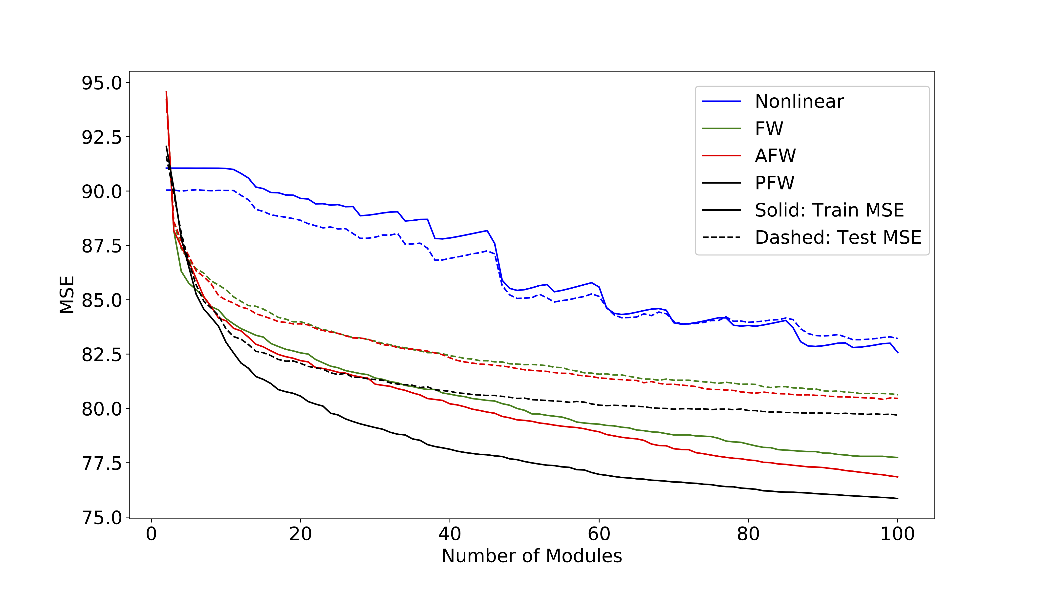
Figure 1: Performance of different variants of the greedy algorithm on msd dataset. Mean squared error against number of modules added to the convex combination. Solid and dashed curves indicate training and test errors respectively.

5.2 Comparison of GCE with Other Algorithms

We compare GCE (using PFW to greedily choose new basis functions), NGCE, XGB, RF, and NN below.

Experimental setup. To ensure a fair comparison between algorithms, we spent a significant effort to tune hyper-parameters of competing algorithms. Particularly, XGB and RF are tuned over 2000 hyper-parameters combinations for small datasets (has less than 10000 training samples), and over 200 combinations for large datasets.

The basis module for GCE is a two-layer network with 1 or 10 hidden neurons for small datasets and 100 hidden neurons for other datasets. GCE grows the network by adding one basis module at a time until no improvement on validation set is detected, or until reaching the maximum limit of 100 modules. NGCE and NN are given the maximum capacity achievable by GCE. For NGCE, it is 100 modules, each of 10/100 hidden neurons for small/large datasets. NN is a two layers neural net of 1000/10000 hidden neurons for small/large datasets, respectively. NGCE and NN are tuned using grid search over learning_rate $\in\{0.01,0.001\}$, regularization $\in\{0,10^{-6},\dots,10^{-1}\}$, totaling in 14 combinations. GCE uses a fixed set of hyper-parameters without tuning: learning_rate$=0.001$, regularization$=0$. All these three algorithms use ReLU activation, MSE criterion for training regression problem, cross entropy loss for classification. The training uses Adam SGD with learning_rate reduced by 10 on plateau (training performance did not improve for 10 consecutive epochs) until reaching the minimum learning_rate of $10^{-5}$, at which point the optimizer is ran for another 10 epochs and then returns the solution with the best performance across all training epochs.

Results and Discussion. For each algorithm, the model using the hyper-parameters with the best validation performance is selected. Its test set performance is reported in Table 1. We ran the experiments on train/test splits fixed across all methods in comparison, instead of using multiple train/test splits, which can be useful for further comparison, but is beyond our computing resources.

Datasets	GCE	XGB	RF	NN	NGCE
diabetes	42.706	46.569	49.519	43.283	44.703
boston	2.165	2.271	2.705	2.217	2.232
ca_housing	0.435	0.393	0.416	0.440	0.437
msd	6.084	6.291	6.462	6.186	7.610
iris	0.00	6.67	6.67	3.33	10.00
wine	0.00	2.78	2.78	0.0	0.0
breast_cancer	3.51	4.39	8.77	3.51	4.39
digits	2.78	3.06	2.50	3.33	3.06
cifar10_f	4.86	5.40	5.16	5.00	4.92
mnist	1.22	1.66	2.32	1.24	1.11
covertype	26.70	26.39	27.73	26.89	26.56
kddcup99	0.01	0.01	0.01	0.01	0.01

Table 1: Summary of the empirical results. MAEs are reported for regression datasets (the first 4 lines), and misclassification rate (%) are reported for classification datasets (last 8 lines). XGBoost and RForest are tuned over more than 2000/200 hyper-parameters combinations for small/large datasets. NN and NGCE are tuned over 14 combinations. GCE grows the model by one basis module at a time and stops when no improvement is detected.

From Table 1, GCE is competitive with the baselines on datasets with different numbers of features and examples. For regression problems, GCE uses up the maximum number of basis functions, while for classification problems, GCE often terminates way earlier than that, suggesting that it is capable to adapt to the complexity of the task.

We have chosen datasets from small to large in our experiments. The small datasets can be easily overfitted, and are useful for comparing how well the algorithms avoid overfitting. Empirical results show that GCE builds up the convex ensemble to just a right capacity, but not more. Thus, it has good generalization performance despite having almost little parameter tuning, even for the smaller datasets, where overfitting could easily occur. On the other extreme, overfitting a very large datasets, like kddcup99, is hard. So, empirical results for this dataset show that all models, including ours, have adequate capacity, as they have similar generalization performance. All algorithms were able to scale to the largest dataset (kddcup99), but GCE usually requires little hyper-parameter tuning, while XGB and RF involve significant tuning.

(a) Comparison of GCE against NN and NGCE. NN and NGCE have very similar performance as GCE on several datasets. NN does not perform well on msd, iris, digits, and cifar10_f, and NGCE does not perform well on diabetes, msd, iris, and breast_cancer. In particular, both NN and NGCE perform poorly on iris. We suspect that NN and NGCE may be more susceptible to local minimum, leading to an underfitted model, and we examined the training and test losses for GCE, NN and NGCE. For several datasets, the differences between the losses of the three algorithms are small, but large differences show up on some datasets. On diabetes and msd, both NGCE and NN seem to underfit, with much larger training and test losses than those of GCE. NGCE and NN seem to overfit boston, with similar test test losses as GCE, but much smaller training loss. NN seems to overfit on iris as well.

NGCE is slightly poorer than NN overall. An unregularized NN usually does not perform well. Since NGCE is trained without any additional regularization (such as $\ell_{2}$ regularization), this suggests that the convex hull constraint has similar regularization effect as a standard regularization, and the improved performance of GCE may be due to greedy training with early stopping.

GCE often learns a smaller model as compared to NGCE and NN on classification problems and does not know the number of components to use a priori. On the other hand, both NGCE and NN requires a priori knowledge of the number of basis functions to use, which is set to be the maximum number of components used for GCE. Finding the best size for a given problem is often hard.

(b) Comparison of GCE against XGBoost and RandomForest. GCE shows clear performance advantage over XGBoost and RandomForest on most domains, except that XGBoost has a clear advantage on ca_housing, and RandomForest performing slightly better on digits.

While RandomForest and XGBoost have quite a few parameters to tune, and a proper tuning often requires searching a large number of hyper-parameters, GCE works well across datasets with a default setting for basis module optimization (no tuning) and two options for module size. Overall, GCE is often more efficient than RandomForest and XGBoost as there is little tuning needed. In addition, for large datasets, RandomForest and XGBoost are slow due to the lack of mechanism for mini-batch training and no GPU speed-up.

6 Conclusion

This paper presents some new results and empirical insights for learning an optimal convex combination of basis models. While we focused on the case with neural networks as the basis models, the greedy algorithms in Section 4 can be applied with trees as basis models. In the case of the nonlinear greedy algorithm and a quadratic loss, the greedy step involves training a regression tree given a fixed step size. For FW variants and other losses, the objective function at each greedy step no longer corresponds to a standard loss function though. Regarding generalization, since trees are nonparametric, our generalization results do not hold, and we may face similar challenges as analyzing random forests. There are interesting questions for further work.

Appendix A Proofs

For a real-valued function $r$ defined on a set ${\mathcal{Z}}$, and a random variable $Z$ taking values from ${\mathcal{Z}}$, we use ${\mathbb{P}}r$ to denote ${\mathbb{E}}r(Z)$, and ${\mathbb{P}}_{n}r$ to denote ${\mathbb{E}}_{n}r(Z)$.

Lemma 1.

(Koltchinskii [2001], Lemma 2.5) Let ${\mathcal{R}}$ be a class of real-valued functions defined on ${\mathcal{Z}}$, then

$${\mathbb{E}}\sup_{r\in{\mathcal{R}}}|{\mathbb{P}}r-{\mathbb{P}}_{n}r|\leq 2{\mathbb{E}}\sup_{r\in{\mathcal{R}}}{\mathbb{R}}_{n}r.$$

Lemma 2.

(Mendelson [2003], Theorem 2.25)

• If $\phi:{\mathbf{R}}\to{\mathbf{R}}$ is $c_{\phi}$-Lipschitz and $\phi(0)=0$, then

  $${\mathbb{R}}_{n}\phi\circ r\leq 2c_{\phi}{\mathbb{R}}_{n}r.$$

• If $g:{\mathcal{Z}}\to[-M,M]$, then

  $${\mathbb{E}}\sup_{r\in{\mathcal{R}}}{\mathbb{R}}_{n}(r+g)\leq{\mathbb{E}}\sup_{r\in{\mathcal{R}}}{\mathbb{R}}_{n}r+\frac{M}{\sqrt{n}}.$$

See 2

Proof.

For any function $f$, define its regret version $r_{f}$ by

$$r_{f}(x,y)=L(y,f(x))-L(y,f^{*}(x)).$$

We call ${\mathcal{R}}=\{r_{f}:f\in{\mathcal{H}}\}$ the regret class of ${\mathcal{H}}$.

For any i.i.d. sample ${\mathbf{z}}=((x_{1},y_{1}),\ldots,(x_{n},y_{n}))$, we first show that $h({\mathbf{z}})=\sup_{r\in{\mathcal{R}}}|{\mathbb{P}}r-{\mathbb{P}}_{n}r|$ is concentrated around its expectation. As a first step, we verify that $h({\mathbf{z}})$ satisfies the bounded difference property with a bound $4c_{\phi}B/n$, as follows. Let ${\mathbf{z}}^{\prime}$ be the same as ${\mathbf{z}}$ except that $(x_{i},y_{i})$ is replaced by an arbitrary $(x^{\prime}_{i},y^{\prime}_{i})\in{\mathcal{X}}\times{\mathcal{Y}}$. Since $\phi$ is $c_{\phi}$-Lipschitz and $\phi(0)=0$, we have

$$L(y,f(x)) =\phi(f(x)-y)-\phi(0)$$

$$\leq c_{\phi}|f(x)-y-0|$$

$$\leq 2c_{\phi}B,$$

thus we have

$$\quad\left|h({\mathbf{z}})-h({\mathbf{z}}^{\prime})\right|$$

$$=\left|\sup_{r\in{\mathcal{R}}}|{\mathbb{P}}r-{\mathbb{P}}_{n}r|-\sup_{r\in{\mathcal{R}}}|{\mathbb{P}}r-{\mathbb{P}}_{n}^{\prime}r|\right|$$

$$\leq\sup_{r\in{\mathcal{R}}}|{\mathbb{P}}_{n}r-{\mathbb{P}}_{n}^{\prime}r|$$

$$=\sup_{f\in{\mathcal{H}}}\frac{1}{n}\bigg{|}\left(L(y_{i},f(x_{i}))-L(y_{i},f^{*}(x_{i}))\right)$$

$$\qquad-\left(L(y_{i}^{\prime},f(x_{i}^{\prime}))-L(y_{i},f^{*}(x_{i}))\right)\bigg{|}$$

$$\leq\frac{4c_{\phi}B}{n}.$$

Hence $h({\mathbf{z}})$ satisfies the bounded difference property with a bound $4c_{\phi}B/n$. By McDiarmid’s inequality, with probability at least $1-\delta$,

$$\sup_{r\in{\mathcal{R}}}|{\mathbb{P}}r-{\mathbb{P}}_{n}r|\leq{\mathbb{E}}\sup_{r\in{\mathcal{R}}}|{\mathbb{P}}r-{\mathbb{P}}_{n}r|+\frac{\sqrt{8c_{\phi}^{2}B^{2}\ln(1/\delta)}}{\sqrt{n}}.$$ (I)

By 1, we have

$${\mathbb{E}}\sup_{r\in{\mathcal{R}}}|{\mathbb{P}}r-{\mathbb{P}}_{n}r|\leq 2{\mathbb{E}}\sup_{r\in{\mathcal{R}}}{\mathbb{R}}_{n}r.$$ (II)

The Rademacher complexity can be bounded as follows

$$\qquad{\mathbb{E}}\sup_{r\in{\mathcal{R}}}{\mathbb{R}}_{n}r$$

$$={\mathbb{E}}\sup_{f\in\operatorname{co}({\mathcal{G}})}{\mathbb{R}}_{n}r_{f}$$

$$={\mathbb{E}}\sup_{f\in\operatorname{co}({\mathcal{G}})}{\mathbb{R}}_{n}(L(\cdot,f(\cdot))-L(\cdot,f^{*}(\cdot)))$$

$$\leq{\mathbb{E}}\sup_{f\in\operatorname{co}({\mathcal{G}})}{\mathbb{R}}_{n}\phi(f(\cdot)-\cdot)+\frac{2c_{\phi}B}{\sqrt{n}}$$

$$\leq 2c_{\phi}{\mathbb{E}}\sup_{f\in\operatorname{co}({\mathcal{G}})}{\mathbb{R}}_{n}(f(\cdot)-\cdot)+\frac{2c_{\phi}B}{\sqrt{n}}$$

$$\leq 2c_{\phi}{\mathbb{E}}\sup_{f\in\operatorname{co}({\mathcal{G}})}{\mathbb{R}}_{n}f+\frac{2Bc_{\phi}}{\sqrt{n}}+\frac{2c_{\phi}B}{\sqrt{n}}$$

$$=2c_{\phi}{\mathbb{E}}\sup_{f\in\operatorname{co}({\mathcal{G}})}{\mathbb{R}}_{n}f+\frac{4c_{\phi}B}{\sqrt{n}},$$

where 1st and 3rd inequalities follow from 2 (b), and 2nd inequality from 2 (a).

We bound the Rademacher complexity ${\mathbb{E}}\sup_{f\in G}{\mathbb{R}}_{n}f$ using a covering number argument, as follows. For any sequence ${\mathbf{x}}=(x_{1},\ldots,x_{n})\in{\mathcal{X}}^{n}$, any $f,g\in{\mathcal{H}}$, let $d_{{\mathbf{x}}}(f,g)=\left(\frac{1}{n}\sum_{i}(f(x_{i})-g(x_{i}))^{2}\right)^{1/2}$. Since $d_{P}({\mathcal{G}})=p$, for any ${\mathbf{x}}$,

$$N(\epsilon,{\mathcal{G}},d_{{\mathbf{x}}})\leq\left(\frac{C}{\epsilon}\right)^{2p},$$ (5)

where $C>0$ is an absolute constant. Using Dudley’s entropy integral bound, we have $\displaystyle{\mathbb{E}}\sup_{f\in G}{\mathbb{R}}_{n}f\leq C^{\prime}B{\mathbb{E}}_{{\mathbf{z}}}\int_{0}^{\infty}\sqrt{\frac{\ln N(\epsilon,G,d_{{\mathbf{x}}})}{n}}d\epsilon=DB\sqrt{p/n}.$ (IV) where $C^{\prime}$ and $D$ are absolute constants.

Combining the inequalities (I)-(IV), we have with probability at least $1-\delta$, for any $r\in{\mathcal{R}}$, we have

$${\mathbb{P}}r\leq{\mathbb{P}}_{n}r+\sup_{r^{\prime}\in{\mathcal{R}}}|{\mathbb{P}}r^{\prime}-{\mathbb{P}}_{n}r^{\prime}|\\ \leq{\mathbb{P}}_{n}r+\frac{2c_{\phi}B\left(\sqrt{2\ln(1/\delta)}+D\sqrt{p}+2\right)}{\sqrt{n}}.$$

∎

See 3 Proof sketch. By inspecting the proof of 3, we can see that the proof still works if we replace $f^{*}$ by an arbitrary function, including $h^{*}$. Thus with probability at least $1-\delta$, we have

$$R(\hat{f})-R(h^{*})\leq R_{n}(\hat{f})-R_{n}(h^{*})+\frac{c}{\sqrt{n}}\leq\frac{c}{\sqrt{n}}.$$

$\square$

See 1

Proof.

We have $L(y,f(x))=\phi(f(x)-y)$ where $\phi(u)=|u|^{q}$. $\phi(u)$ has a Lipschitz constant of $q(2B)^{q-1}$ in our case, because we only consider $u$ of the form $f(x)-y$, and thus $u\in[-2B,2B]$, and for any $u,v\in[-2B,2B]$, we have $|\phi(u)-\phi(v)|=|qc^{q-1}(|u|-|v|)|\leq q(2B)^{q-1}|u-v|$, where $c$ is between $|u|$ and $|v$. The first equation is obtained by applying the mean value theorem to the function $u^{p}$, and taking absolute values on both sides. The second inequality follows because both $|u|$ and $|v|$ are not more than $2B$, and $||u|-|v||\leq|u-v|$. ∎

See 2 Proof sketch. First note that the loss $L$ is bounded by $c_{\phi}B$ because $\phi$ is Lipschitz, $\phi(0)=0$, and the margin $yf(x)$ is in $[-B,B]$. Thus $L$ is also bounded by $2c_{\phi}B$. This allows the McDiarmid’s inequality in the proof of 2 to go through. Secondly, Eq. (*) in the proof of 2 becomes

$${\mathbb{E}}\sup_{f\in\operatorname{co}({\mathcal{G}})}{\mathbb{R}}_{n}\phi(\cdot f(\cdot))+\frac{2c_{\phi}B}{\sqrt{n}},$$

where the first $\cdot$ is the output $y$, and the second $\cdot$ is the input $x$. Now we can apply the Lipschitz property of $\phi$ to bound the first term by $2c_{\phi}{\mathbb{E}}\sup_{f\in\operatorname{co}({\mathcal{G}})}{\mathbb{R}}_{n}\cdot f(\cdot)$. This is equal to $2c_{\phi}{\mathbb{E}}\sup_{f\in\operatorname{co}({\mathcal{G}})}{\mathbb{R}}_{n}f(\cdot)$, because $y\in\{-1,1\}$. Thus the bound (III) still holds. The remaining steps go through without any modification. $\square$

See 3

Proof.

Consider the loss $L^{\prime}(y,f(x)=-\ln\frac{2}{1+e^{-yf(x)}}$. Then $L^{\prime}(y,f(x))=L(y,f(x))-\ln 2$, that is, $L$ and $L^{\prime}$ differ by only a constant, and thus it is sufficient to show that the bound holds for $L^{\prime}$. The modified loss $L^{\prime}(y,f(x))$ has the form $\phi(yf(x))$ where $\phi(u)=-\ln\frac{2}{1+e^{-u}}$. We have $\phi(0)=0$. In addition, $\phi$ is 1-Lipschitz because the absolute value of its derivative is $|\phi^{\prime}(u)|=|\frac{-e^{-u}}{1+e^{-u}}|\leq 1$. Hence $L^{\prime}$ satisfies the condition in 2, and the $O(1/\sqrt{n})$ bound there holds for $L^{\prime}$. ∎

Appendix B Datasets and Experimental Setup

We used 12 datasets of various sizes and tasks (both regression and classification) in the experiments. Most of the datasets are from UCI ML Repository [Dheeru and Karra Taniskidou, 2017]. Table 2 provides a summary of the datasets.

datasets	task	#dim	#samples	#train	#valdtn	#test
diabetes	regr	10	442	282	71	89
boston	regr	13	506	323	81	102
ca_housing	regr	8	20,640	13,209	3,303	4,128
msd	regr	90	515,345	†296,777	74,195	†144,373
iris	class	4	150	96	24	30
wine	class	13	178	113	29	36
breast_cancer	class	30	569	364	91	114
digits	class	64	1,797	1,149	288	360
cifar10_f	class	342	60,000	†32,000	8,000	†20,000
mnist	class	784	70,000	†38,400	9,600	†22,000
covertype	class	54	581,012	†11,340	†2,268	†569,672
kddcup99	class	41	4,898,431	†2,645,152	661,288	†1,591,991

Table 2: Summary of datasets used in the experiments. ^‡: number of classes for classification and $\max|output|$ for regression. ^†: a predefined set chosen by the author of the respective dataset. If not predefined, training/test set is a random split of 80%/20% of the dataset. Then, the training set is again split into 80% for training and 20% for validation. boston, diabetes, iris, digits, wine, breast_cancer, covertype, kddcup99, ca_housing are loaded using data utility in scikit-learn package. (Year prediction) msd is taken directly from UCI’s website. mnist and cifar10 are well known datasets and are loaded using PyTorch data utilities. cifar10_f is created by transforming cifar10 using a trained DenseNet (95.16% accuracy on test set) and taking the values of 342 features in the last convolutional layer. Training/validation/test set remain identical across all experiments. All data attributes are normalized to have 0-mean 1-standard deviation.

To ensure a fair comparison between algorithms, we spent a significant effort to tune the hyper-parameters of competing algorithms. For each algorithm, the model with the best validation performance is selected and the performance on test set is reported. Small datasets (less than 10000 training samples, i.e. boston, diabetes, iris, digits, wine, breast_cancer), allow for a larger number of hyper-parameter tuning combinations. The details of hyper-parameter tuning for each algorithm is as follows:

• XGBoost: Evaluation metric eval_metric=merror for classification and eval_metric=rmse for regression. num_boost_round=2000, early_stopping_rounds=50. For small datasets, we start with eta=0.1 and do 100 random searches over the two most important hyper-parameters in the following ranges: max_depth $\in\{3,5,7,9,11,13\}$, min_child_weight $\in\{0,2,4,6,8,10,12,14,16,18\}$. The random search is followed by a $5\times 5$ fine tuning grid search around the best value for each parameters. Next, we tune gamma $\in\{0.0,0.1,0.2,0.3,0.4,0.5\}$, followed by a grid search for subsample $\in\{0.5,0.6,0.7,0.8,0.9\}$ and colsample_bytree $\in\{0.5,0.6,0.7,0.8,0.9\}$, followed by another grid search for reg_lambda $\in\{0,0.0001,0.001,0.01,0.1,1,10,100\}$ and reg_alpha $\in\{0,0.1,1\}$. Next, we tune the learning rate eta $\in\{0.2,0.15,0.05,0.01,0.005,0.001\}$. Then finally we do a 1000 random searches in the neighborhood of the best value for all parameters. This process generates in total about 2298 combinations of hyper-parameters settings. For large datasets, the procedure is similar, with more restrictive range of values for secondary parameters: gamma $\in\{0,0.05,0.1,0.2\}$, subsample $\in\{0.5,0.6,0.7,0.8\}$, colsample_bytree $\in\{0.5,0.6,0.7,0.8\}$, reg_lambda $\in\{0,0.5,1,1.5\}$, eta $\in\{0.15,0.05,0.01\}$, which are also optimized separately instead of jointly in pairs as before.

• RandomForest: Training criterion is $gini$ for classification and $mse$ for regression. The maximum number of trees is 2000, with early stoping if there is no improvement over 50 additional trees. For Random Forest, we found that a large number of random searches is often the most effective strategy. So, we do 4000/200 random searches for small/large datasets respectively. The hyper-parameters and their range are as follows.
  max_features $\in\{auto,sqrt,log2,1,3,5,0.1,0.2,0.3,\\ 0.4,0.5,0.6,0.7\}$,
  min_samples_leaf $\in\{1,2,5,10,20,30,50,80,120,170,\\ 230\}$,
  max_depth $\in\{1,2,5,10,20,30,50,80,120\}$,
  min_samples_split $\in\{2,4,6,8,10,12,14,16\}$,
  no_bootstrap $\in\{True,False\}$.

• GCE, NGCE, NN: The basis module for GCE is a two layers network with 1 or 10 hidden neurons for small datasets and 100 hidden neurons for other datasets. The output of the basis module is bounded using the $hardtanh$ function scaled by the bound $B$. For classification we set $B=10$, for regression, $B=\frac{4}{3}\max|output|$. GCE grows the network by adding one basis module at a time until no improvement on validation set is detected, or until reaching the maximum limit of 100 modules. We use Brent’s method as line search for parameter $\alpha_{t}$ of GCE. NGCE and NN are given the maximum capacity achievable by GCE. For NGCE, it is 100 modules, each of 10/100 hidden neurons for small/large datasets. NN is a two layers neural net of 1000/10000 hidden neurons for small/large datasets, respectively. For both small and large datasets, NGCE and NN are tuned using grid search over $learning\_rate\in\{0.01,0.001\}$, $regularization\in\{0,10^{-6},\dots,10^{-1}\}$, totaling in 14 combinations. GCE uses a fixed set of hyper-parameters without tuning: $learning\_rate=0.001,regularization=0$. All these three algorithms use ReLU activation, MSE criterion for training regression problem, cross entropy loss for classification. The training uses Adam SGD with $learning\_rate$ reduced by 10 on plateau (training performance did not improve for 10 consecutive epochs) until reaching the minimum learning rate of $10^{-5}$, at which point the optimizer is ran for another 10 epochs and then returns the solution with the best performance across all training epochs.

All experiments are implemented using Python and its interface for XGBoost. Random Forest is from scikit-learn package. Greedy variants and NN are implemented using PyTorch [Paszke et al., 2017] and are ran on a machine with Intel i5-7600K CPU @ 3.80GHz (4 cores) and 1x NVIDIA GEFORCE GTX 1080 Ti GPU card. XGBoost and Random Forest are run on cloud machines with Intel CPU E5-2650 v3 @ 2.30GHz (8 cores) and one NVIDIA GEFORCE RTX 2080 Ti GPU.