Large-scale Gastric Cancer Screening and Localization
Using Multi-task Deep Neural Network

Abstract

Gastric cancer is one of the most common cancers, which ranks third among the leading causes of cancer death. Biopsy of gastric mucosa is a standard procedure in gastric cancer screening test. However, manual pathological inspection is labor-intensive and time-consuming. Besides, it is challenging for an automated algorithm to locate the small lesion regions in the gigapixel whole-slide image and make the decision correctly. To tackle these issues, we collected large-scale whole-slide image dataset with detailed lesion region annotation and designed a whole-slide image analyzing framework consisting of 3 networks which could not only determine the screening result but also present the suspicious areas to the pathologist for reference. Experiments demonstrated that our proposed framework achieves sensitivity of $97.05\%$ and specificity of $92.72\%$ in screening task and Dice coefficient of $0.8331$ in segmentation task. Furthermore, we tested our best model in real-world scenario on $10,315$ whole-slide images collected from $4$ medical centers.

1 Introduction

Gastric cancer remains important cancer worldwide and is responsible for over $1,000,000$ new cases in 2018 and an estimated $783,000$ deaths (equating to 1 in every 12 deaths globally), making it the fifth most frequently diagnosed cancer and the third leading cause of cancer death. Biopsy of the gastric mucosa is one of the most effective methods of early detection of gastric cancer Bray et al. [2018]. It is estimated that there are hundreds of millions of gastric biopsy slides need to be examined in China each year, while the number of certified pathologists is only about $10$ thousand, which causes excessive workloads on these pathologists.

To reduce the workload of the pathologists, there are extensive studies focus on pathology image analysis Zhang et al. [2014], Xu et al. [2015], Fakhry et al. [2016], Li et al. [2018b], Hu et al. [2018], Duan et al. [2020]. In recent years, deep neural network techniques have achieved remarkable performance on a wide range of computer vision tasks, such as image classification Krizhevsky et al. [2012], He et al. [2016], Szegedy et al. [2016], object detection He et al. [2017], Lin et al. [2017], Redmon and Farhadi [2018], semantic segmentation Long et al. [2015], Chen et al. [2018], etc. These techniques have been applied in automated pathology image analysis in the past few years. Unlike natural images, digital pathology images, named whole-slide images (WSIs), are extremely large whose width and height often exceed $100,000$ pixels. On the other hand, histological diagnosis requires high accuracy since it is commonly considered as the gold standard. As a result, some of the studies focus on the selected regions of interest (ROIs) Su et al. [2015], Zhang et al. [2015b, a], Albarqouni et al. [2016], Chen et al. [2017], Li et al. [2019b, a], while there are several attempts on analyzing WSI Barker et al. [2016], Coudray et al. [2018], Lin et al. [2018], Zhang et al. [2019].

Besides the difficulties in applying the deep neural network on gigapixel resolution images, the main challenge in examining the WSIs is that the diagnostic results labeled by the pathologists are usually on the slide level in most of the publicly available datasets, while the lesion regions that draw the pathologists’ attention are extremely small compared with the size of the WSI. It is tough to train a deep neural network to locate those regions and make the correct decision only using slide level labels such “positive/negative”. Therefore, we collect a large dataset that not only has the slide level annotation but also carries the lesion region annotation and design a framework leveraging the detailed supervised information.

To our best knowledge, there have been no studies on automated pathology image analysis with lesion region annotation for gastric cancer. We propose an automated screening framework that could not only provide the screening results, i.e., positive/negative, but also show the suspicious areas to pathologists for further reference.

2 Related Works

2.1 Pathology Image Analysis for Gastric Cancer

Only a few existing works are focusing on analyzing the pathology image from the biopsy of the gastric mucosa for diagnosis.

Cosatto et al. [2013] designed a semi-supervised multiple instance learning framework that takes $230\times 230$ microns at magnification of $20X$ and $460\times 460$ microns at magnification of $10X$ ROIs segmented from tissue units as input and analyzes their color features.

Oikawa et al. [2017] proposed a computerized analysis system which first analyzes color and texture features on the entire H&E-stained section at low resolution to search suspicious areas for cancer (except signet ring cell which is detected by CNN-based method), and then analyzes contour and pixel features at high resolution on selected area and uses a trained SVM to confirm the initial suspicion.

Li et al. [2018a] proposed GastricNet to automatically identify gastric cancer. The network with different architectures for shallow and deep layers was applied on $224\times 224$ patches cropped from $700$ $2048\times 2048$ ROIs with a magnification factor of $20X$.

Yoshida et al. [2018] compared the classification results of human pathologists and of the e-Pathologist. The e-Pathologist analyzes high-magnification features that characterized the nuclear morphology and texture as well as low-magnification features that characterized the global H&E stain distribution within an ROI and the appearance of blood cells and gland formation. The classification was modeled as a multi-instance learning problem and solved by training a multi-layer neural network.

2.2 Whole-Slide Image Analysis

As the gold standard for various cancer diagnosis, WSIs analysis related techniques have been well-studied in recent years.

Liu et al. [2017] presented a CNN framework to aid breast cancer metastasis detection in lymph nodes. The model is based on Inception architecture with careful image patch sampling and data augmentations. Random forest classifier and feature engineering were used for whole-slide classification procedure.

Hou et al. [2016] proposed to train a decision fusion model to aggregate patch-level predictions given by patch-level CNNs. In addition, authors formulated a Expectation-Maximization based method that automatically locates discriminative patches robustly by utilizing the spatial relationships of patches.

Zhu et al. [2017] proposed a survival analysis framework which first extract hundreds of patches by adaptive sampling and then group these images into different clusters. An aggregation model was trained to make patient-level predictions based on cluster-level results.

Mercan et al. [2017] developed a framework to analyze breast histopathology image. Candidate ROIs were extracted from the logs of pathologists’ image screenings based on different behaviors. Class labels were extracted from the pathology forms and slides were modeled as bags of instances which are represented by the candidate ROIs.

Localizing of lesion regions in WSIs by image segmentation related techniques is also a crucial direction for helping pathologists make the correct decision efficiently.

Qaiser et al. [2019] proposed a tumor segmentation framework based on the concept of persistent homology profiles which models the atypical characteristics of tumor nuclei to localize the malignant tumor regions. Dong et al. [2018] proposed a reinforcement learning based framework motivated by the zoom-in operation of a pathologist which learns a policy network to decide whether zooming is required in a given ROI.

Our main contributions:

• We collect a large-scale dataset for gastric cancer screening and develop a semi-automated annotation system to help obtain the detailed lesion region annotation.

• We take advantage of the region annotation by proposing a multi-task network structure which could provide the classification label (screening result) as well as the segmentation mask (suspicious region) simultaneously.

• We design a practical framework consisting of $3$ networks to process the high-resolution WSIs, and employ the deformable convolution operation based on the observation of the characteristics of the pathology images.

3 Data Collection

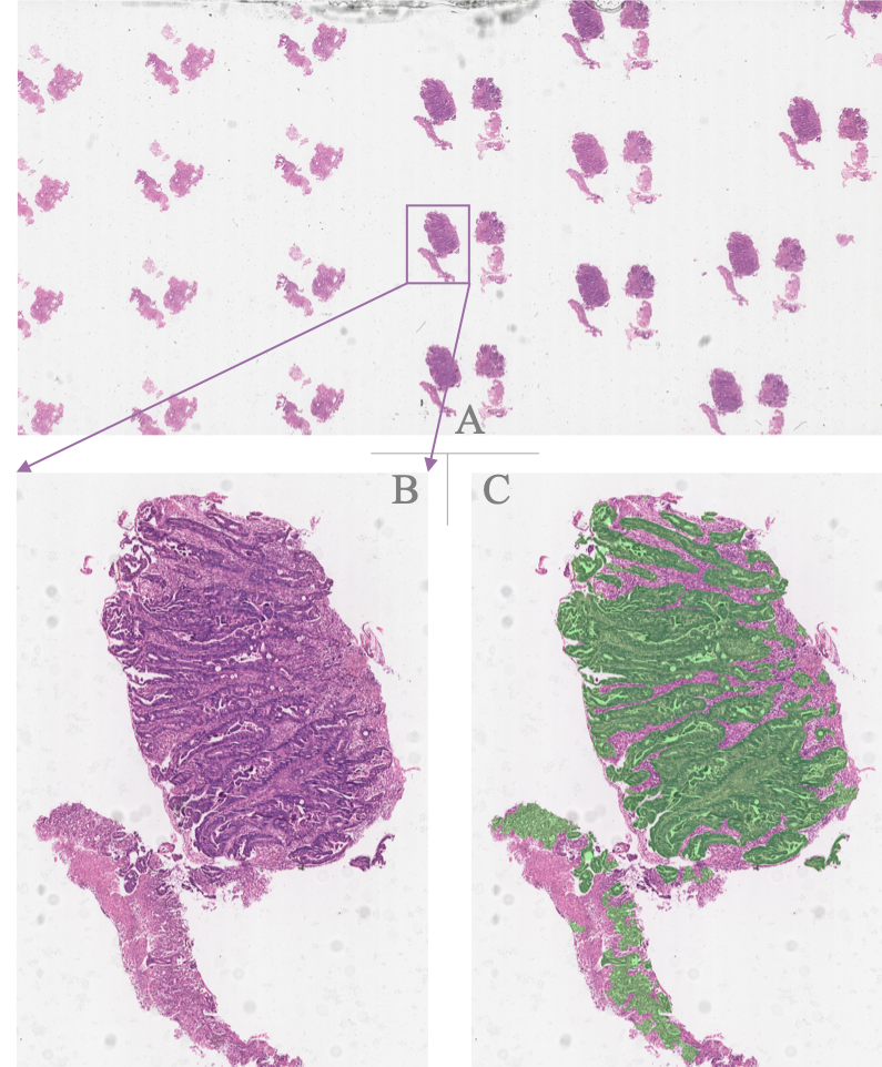
Figure 1: A) A typical WSI of gastric biopsy. Pathologists usually cut all the suspicious tissues of gastric mucosa acquired from gastroscope into multiple thin sections and put it on a single glass slide. Hence, sections on the same slide could be the adjacent part of the same tissue or even different tissues. B) One of the enlarged regions of WSI. There are some irregular textures and muscularis mucosae. C) Lesion region annotation. The region considered as malignant is denoted by the green overlay.

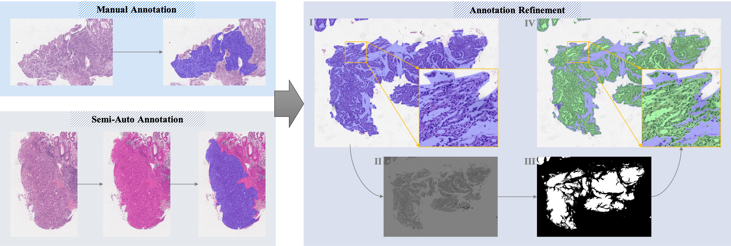
Figure 2: Our annotation pipeline. The pipeline consists of two parts, namely the initial annotation and the refinement. The initial annotation part (on the left) has two routes: manul annotation (blue overlay) and semi-auto annotation (pink denotes the output of the U-Net, blue denotes the annotation after pathologists’ editing). The refinement part (on the right) shows I) the annotation from pathologists (blue), II) output of color deconvolution, III) binary image after applying Otsu thresholding. IV) the final ground truth annotation (green) after refinement.

3.1 Data Acquisition

All the annotated slides are automatically scanned using the digital pathology scanner Leica Aperio AT2 at $20X$ magnification ($0.50um/pixel$) and labeled by pathologists under the supervision of the experts in Shanghai General Hospital.

The slide-level annotation is either “positive” (refers to the malignant sample such as low-grade intraepithelial neoplasia, high-grade intraepithelial neoplasia, adenocarcinoma, signet ring cell carcinoma, and poorly cohesive carcinoma) or “negative” (refers to the benign sample such as chronic atrophic gastritis, chronic non-atrophic gastritis, intestinal metaplasia, gastric polyps, gastric mucosal erosion, etc) by the pathologists according to whether the follow-up examination and treatment are needed. All the malignant regions are labeled along with their contours and converted to a mask. (Shown in Figure. 1.)

3.2 Semi-automated Annotation System

The manual annotation procedures designed by the experts of Shanghai General Hospital are:

1. Coarse labeling. The pathologist finds the suspicious area in the high-resolution gigapixel image and selects them with bounding boxes.

2. Fine labeling. Within the selected bounding box, pathologist further confirms whether it is malignant, draws a closed curve along the contour of the malignant region and marks the lesion type of the region.

3. Double checking. Finally, the experts go through all the annotated WSIs and verify the correctness of the labels.

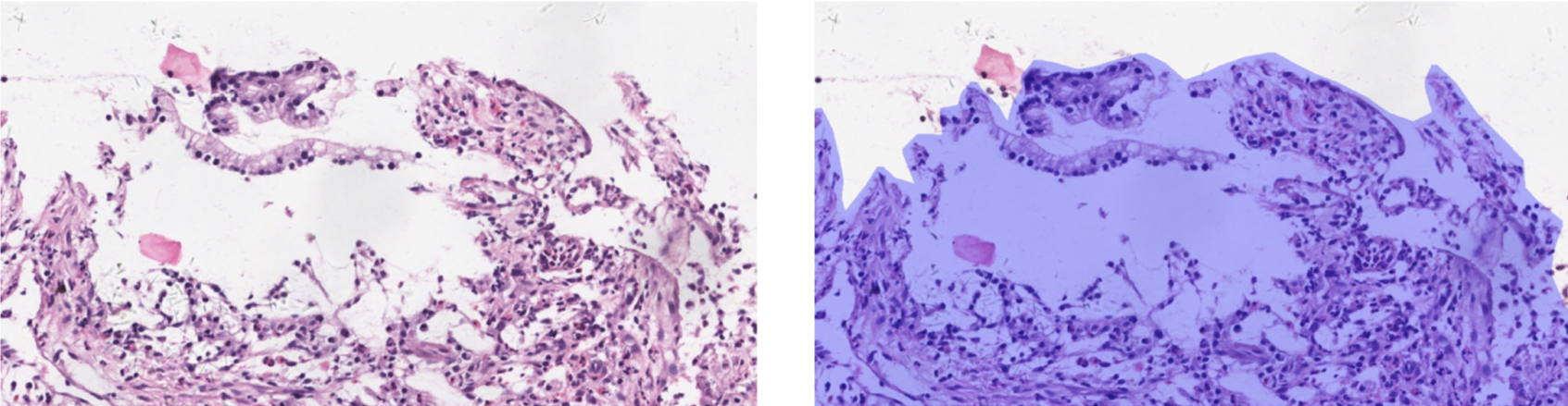
Figure 3: An enlarged part of WSI. Blue overlay in the right image denotes the manual annotation from the pathologist, which may cover many empty regions.

Manually labeling a WSI usually takes $1-3$ hours and the contour may not align perfectly with the border due to the enormous image size and the highly unsmooth edge (shown in Figure. 3).

To address this issue, we introduce a semi-automated annotation system (shown in Figure. 2). An annotation refinement module with a series of image processing techniques is employed to eliminate the background areas in the manually labeled regions (shown in the right part of Figure. 2). Color deconvolution technique Van der Laak et al. [2000], Ruifrok et al. [2001] is used to extract Hematoxylin & Eosin-stained regions (image II). Based on the output of color deconvolution, we could obtain the foreground by applying Otsu thresholding Otsu [1979] (image III). The final segmentation annotations are the intersection between the foregrounds and the pathologists annotated areas (image IV). These procedures could fix the empty regions and loose boundary without modifying the true malignant region.

As shown in the left part of Figure. 2, we further propose to initialize a preliminary annotation with the output of a segmentation network trained on a few labeled WSIs. Then, pathologists only need to modify the masked regions discovered by the segmentation network, which could effectively speed up the labeling procedure. Basically, our semi-automated annotation system could generate more accurate region contours and reduce the labeling time to $~{}20$ minutes.

With the protocol and semi-automated tools designed for acquiring data, we collected $518$ WSIs with both slide-level labels and detailed region annotation from Shanghai General Hospital in the year of 2018. Among these WSIs, $207$ are labeled positive, and $311$ are labeled negative.

3.3 Large-scale Dataset from Multiple Institutes

Moreover, in order to test the generalizability of our proposed model in real-world scenario, we collected $10,315$ WSIs with slide-level screening labels from four hospitals in East China, i.e., Sijing Hospital of Shanghai Songjiang District (SHSSD), Songjiang District Center Hospital (SDCH), Zhejiang Provincial People’s Hospital (ZPPH) and Shanghai General Hospital (SGH). These hospitals have their own pathology slide preparation procedures, which make the WSIs have different tissue thicknesses and color tones.

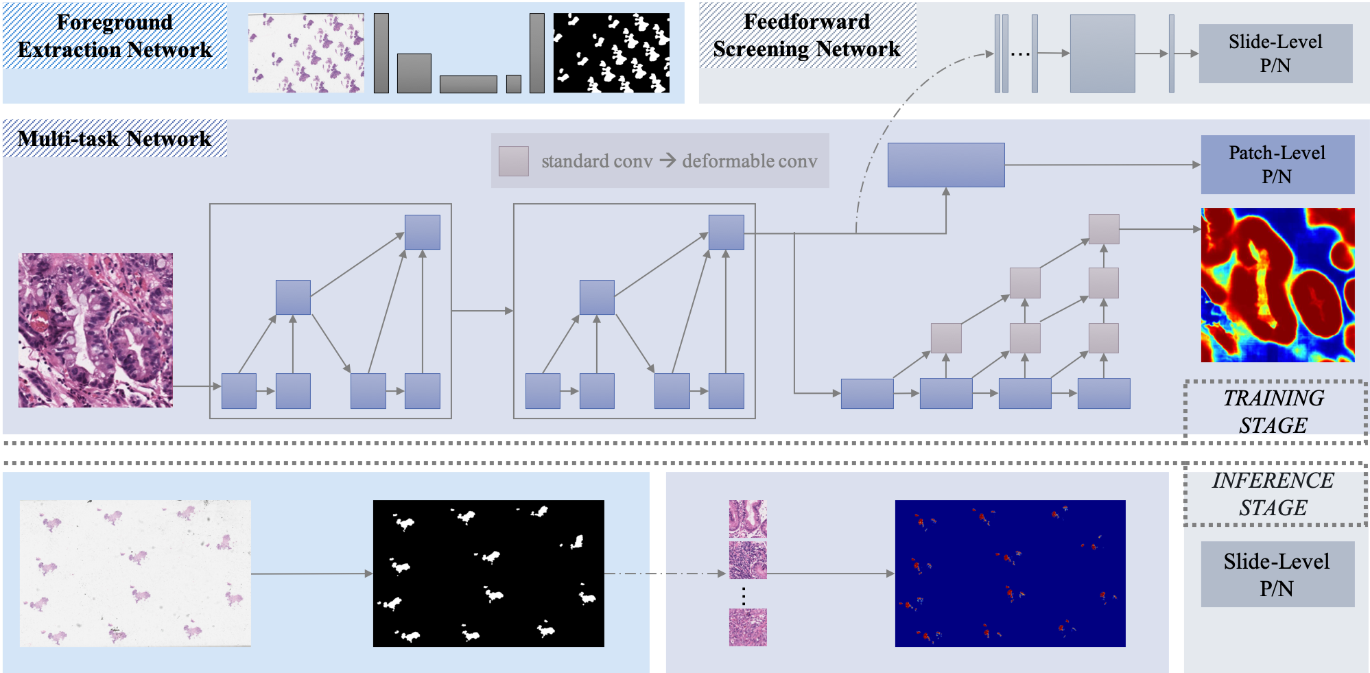
Figure 4: The overview of our proposed gastric cancer screening framework. On the top, we show the structure of the proposed foreground extraction network, multi-task network, and feedforward screening network, which are trained separately during the training stage. The inference stage is illustrated in the bottom. The mask is obtained by the foreground extraction network. Then the patches cropped from the foreground are send to the multi-task network for classification and segmentation. Finally, the feature vectors from the second network are collected and fed to the screening network to produce the slide-level result.

4 Methods

The main challenge in analyzing WSIs is that the images are extremely large, while only a small part of images contains the lesion region. Hence, we propose a gastric cancer screening and localization framework (shown in Figure. 4), which consists of 1) a lite segmentation network for extracting the tissue region and eliminating the background area, 2) a multi-task network for generating classification and segmentation results for every cropped patch, and 3) a simple feedforward network for providing the slide-level screening result.

4.1 Network Structure

Multi-task Network. We employ deep layer aggregation (DLA) structure Yu et al. [2018] as the backbone since it is designed to aggregate layers to fuse semantic and spatial information for better recognition and localization. In our case, we utilize the dense prediction network for lesion region segmentation and change it to a multi-task structure by adding a classification branch on the output of the encoder. In the training phase, we use the patches cropped from ROIs with their annotated malignant region masks as the positive inputs and the patches randomly cropped from the benign region with the background (all-zero) masks as the negative inputs, and train the network in an end-to-end manner by combining the classification loss and the segmentation loss (Equation. 1). In the inference phase, patches from each sliding window are sent to the network to generate the classification score and the segmentation heatmap.

$$L=\lambda L_{cls}+L_{seg}$$ (1)

where $L_{cls}$ denotes the loss in classification branch, $L_{seg}$ is the binary cross entropy loss in segmentation branch, and $\lambda$ is a hyper-parameter to balance the weights of these two losses.

Feedforward Screening Network. The input of this network is a matrix $\mathbf{X}\in\mathbb{R}^{k\times d}$ which consists of the mid-layer features (i.e., the output of encoder) $\mathbf{x}\in\mathbb{R}^{1\times d}$ in the dense prediction DLA structure from $k$ patches with the highest probability of being malignant. The network contains a $1\times 1$ convolution layer with a ReLU layer, a max-pooling operation along the sample axis which generates a $\mathbf{Y}\in\mathbb{R}^{1\times d}$ tensor, and a fully connected layer followed by a sigmoid function. Ground truth label of this network is defined in a multi-instance learning (MIL) manner, i.e., whether the WSI contains at least one malignant region.

Since lesion regions only account for $20\%$ percent of the tissue or less, it is difficult for a network targeting at recognition task such as as Krizhevsky et al. [2012], He et al. [2016], Szegedy et al. [2016] to find where to pay attention. In this project, we could take advantage of the detailed lesion region annotation. The multi-task network is designed for producing patch-level results. The segmentation task could not only generate the lesion region mask but also help the whole network locate the regions that really need to focus, which could implicitly support the classification branch to achieve higher performance. The feedforward screening network is proposed for generating the slide-level results. The basic idea in designing this simple feedforward network follows the concept of MIL.

Because the gastric WSIs usually carry many blank areas. We further design a foreground extraction network to extract all tissue region and reduce the running time in the inference phase. It is a segmentation network with $4$ convolution layers and $1$ upsampling layer. The ground truth masks are firstly generated by color deconvlotion Van der Laak et al. [2000], Ruifrok et al. [2001] and Otsu thresholding Otsu [1979]. Then we manually go through all the algorithm generated masks and delete failure cases caused by some unusual problems such as shadows on the edge of the slides. The input of this network are the resized WSIs from the lowest magnification level (i.e., $\times 0.635$). The output of this network is utilized in the inference stage for selecting the sliding window area.

4.2 Deformable Convolution

Another issue in WSIs is that the lesion regions often come with irregular shapes and various sizes while standard convolution operation always fails to handle large geometric transformations due to the fixed geometric structures. Therefore, instead of using standard convolution operation, we employ the deformable convolution layer Dai et al. [2017] in the decoder.

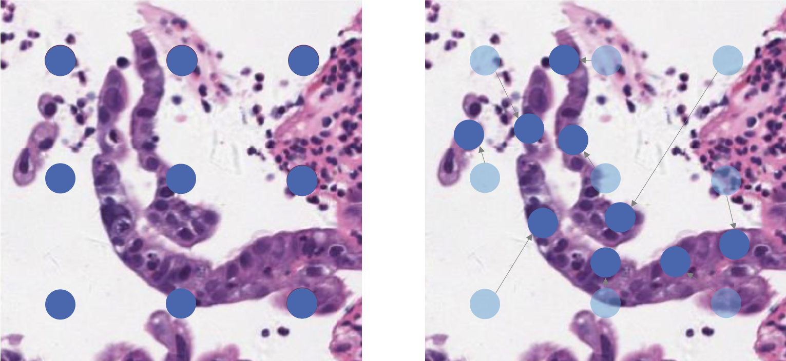
Figure 5: Left: standard convolution operator. Right: deformable convolution operator.

Deformable convolution is proposed based on the idea of augmenting the spatial sampling locations in the modules with additional offsets:

$$y(p_{0})=w(p_{n})\cdot x(p_{0}+p_{n}+\Delta p_{n})$$ (2)

where $x$ denotes the input feature map, $y$ denotes the output feature map, $p_{0}$ is a location on input feature map, $p_{n}\in\mathcal{R}$ and $\mathcal{R}$ is a regular grid $\mathcal{R}={(-1,-1),(-1,0),\dots,(0,1),(1,1)}$. This type of convolution operation allows adding 2D offsets $\Delta p_{n}$ to the regular grid sampling locations $p_{0}+p_{n}$ in the standard convolution.

As demonstrated in Figure. 5, we could easily benefit from the adaptive receptive field when handling the lesion regions with irregular shapes. The deformable convolution operation enables free form deformation of the sampling grid by adding additional offsets (the arrows in the right image of Figure. 5). The offsets are learned from the segmentation task simultaneously with convolutional kernels during training. Hence, the deformation is conditioned on the input features in a local, dense, and adaptive way.

As a consequence, we could capture the feature of the tissue regions with various shapes by utilizing deformable convolution operation, which leads to better performance on the segmentation task.

5 Evaluation

5.1 Implementation Details

We choose the basic DLA-34 with dense prediction part as the backbone of the multi-task network, replace the first $7\times 7$ convolution layer with three $3\times 3$ convolution layers, and several standard convolution layers in decoder with $3\times 3$ deformable convolution layers. Besides, in-place activated batch normalization Rota Bulò et al. [2018] is employed to reduce the memory requirement in training deep networks.

All WSIs are resized to $512\times 512$ for foreground extraction. The input patch size of multi-task network is also set to $512\times 512$. The output of the classification branch of this network is a $512$ feature vector.

The $\lambda$ in Equation. 1 used for balancing the classification loss and segmentation loss is set to $0.01$. The hyper-parameters in the feedforward screening network are selected by cross-validation. We pick $k=64$ to form a $64\times 512$ matrix as the input of the feedforward screening network. Threshold of feedforward screening network is set to $0.74$, i.e., the WSI should be considered as positive if the output of the sigmoid function is larger than $0.74$.

We use Adam optimizer to train the networks separately. The initial learning rate is set to $10^{-3}$ and reduced by a factor $0.5$ when the validation loss stagnates for $3$ epochs. The foreground extraction network is trained for $100$ epochs with the batch size $32$ on one GPU. The multi-task network is trained for $100$ epochs with the batch size $16$ on $4$ GPUs with $12$GB RAM. And the feedforward screening network is trained for $20$ epochs with the batch size $32$ on a single GPU.

5.2 Evaluation of Segmentation

$21,507$ positive patches are cropped from the annotated $400$ ROIs, and $168,485$ negative patches are collected from the WSIs that are diagnosed as benign. Data augmentation techniques such as horizontal/vertical flip, rotation, random cropping and resizing, changing the aspect ratio and image contrast, and adding Gaussian noise are applied during training. We use repeated random sub-sampling strategy in evaluation. Patches from about $30\%$ WSIs are selected as the testing set by the patient ID, and the whole procedures are repeated $4$ times for stable results.

For the evaluation metric, we use the Dice coefficient (DSC) defined over image pixels.

$$DSC=\frac{2TP}{2TP+FP+FN}$$ (3)

We compare our proposed method with commonly used segmentation networks, i.e., FCN Long et al. [2015], U-Net Ronneberger et al. [2015], and the standard DLA Yu et al. [2018] structure without any modification.

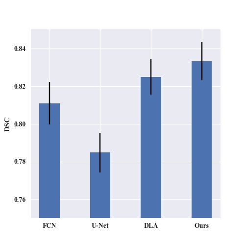
Figure 6: segmentation results of our proposed model and other comparison methods.

FCN and U-Net serve as the baselines, which give us a sense about the performance of commonly used methods on our dataset. Dice coefficient of these two methods is $0.8109\pm 0.0113$ and $0.7847\pm 0.0106$, respectively. The possible reason for FCN performing better could be it benefits more from classification branch without the skip connections like U-Net. DLA performs better, i.e., $0.8248\pm 0.0094$, because it benefits from fusing information by aggregating layers. Our proposed model achieves the highest DSC of $0.8331\pm 0.0101$ as we adjust the standard DLA structure according to our problem settings by replacing the standard convolution with deformable convolution operator.

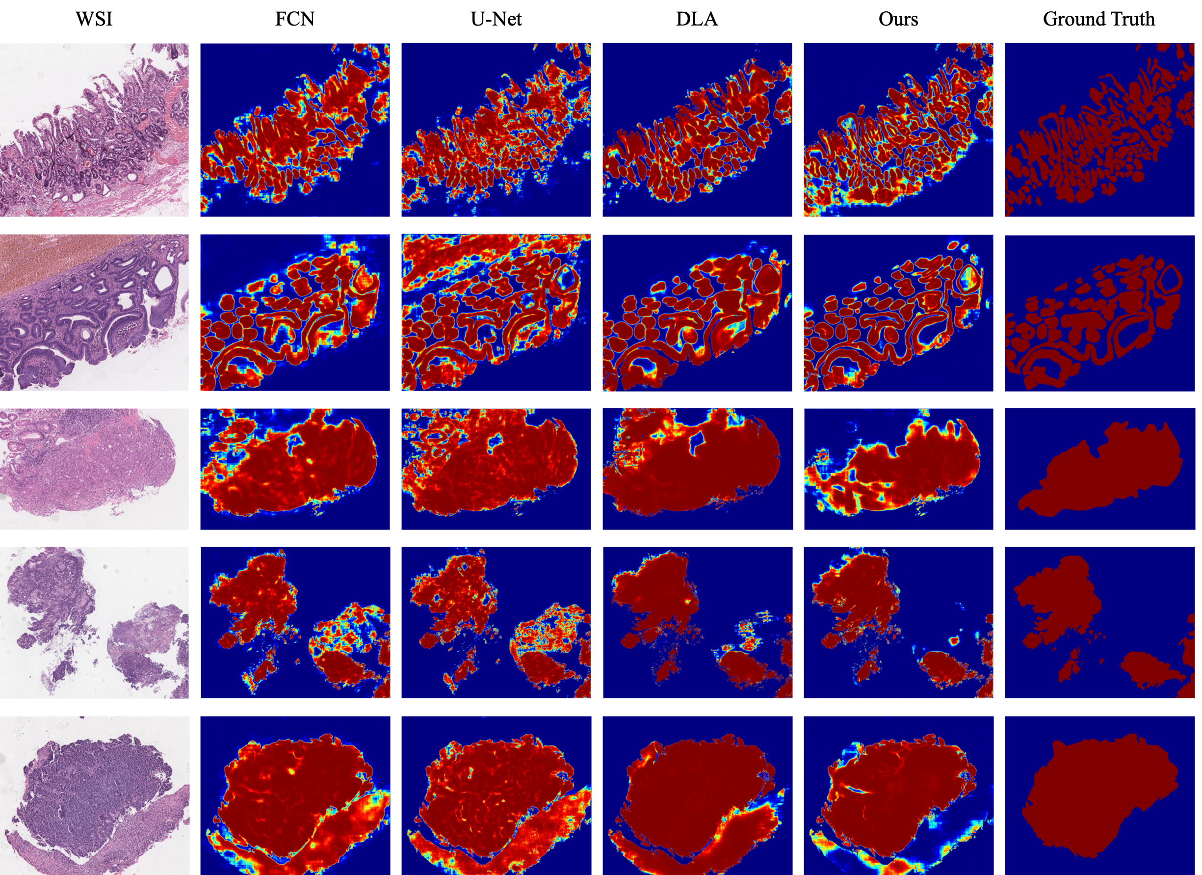
Figure 7: Examples of segmentation results. We show $5$ ROIs with their original image (left) and the ground truth masks (right) labeled by pathologists. Results of our proposed method and other comparison methods are illustrated in the middle columns.

To better demonstrate the effectiveness of our proposed method, we show some examples in Figure. 7. FCN and U-Net often generate unclear and unsmooth boundaries (1st and 2nd row). As we could see from the 3rd to the 5th column, the 3 comparison methods make a lot of false positives compared to our method. In the 2nd row, U-Net even includes red blood cell area in the result. In the 5th row, our model is the only one that successfully identifies the tissue on the bottom to be negative.

5.3 Evaluation of Screening

Compare with the segmentation evaluation that requires a testing set with lesion region annotation, evaluating the screening results of our proposed model could be done on a larger testing set with screening annotation only, i.e., $102$ positive samples and $838$ negative samples.

In Table. 1, we report the screening results of our proposed framework and comparison methods on multiple evaluation metrics, i.e., sensitivity and specificity at the threshold of $0.74$, and Area Under Precision-Recall Curve (AUC). The comparison methods are 1) single task classification networks, such as ResNet He et al. [2016], DenseNet Huang et al. [2017], Res2Net Gao et al. [2019], EfficientNet Tan and Le [2019], and DLA (the same backbone as our proposed network structure); 2) multi-task network structure with different backbones, such as FCN Long et al. [2015] and U-Net Ronneberger et al. [2015].

	Sensitivity	Specificity	AUC
ResNet-34	0.9118	0.9427	0.9017
DenseNet-121	0.9118	0.9463	0.9021
Res2Net-50	0.9314	0.9606	0.9047
EfficientNet-B4	0.9509	0.9653	0.9081
DLA	0.9314	0.9582	0.9038
FCN	0.9608	0.8938	0.9099
U-Net	0.9608	0.8914	0.9117
Ours	0.9705	0.9272	0.9166

Table 1: Screening results of our proposed model compared with other methods.

The primary goal of our proposed framework is gastric cancer screening. In other words, the number of negative samples is much larger than the positive ones (about $9:1$ in this testing set). In this case, sensitivity is the most critical evaluation metric when we take clinical background knowledge into consideration since we would not like to miss any of the malignant cases. Besides, specificity is the second priority because we do not want too many false alarms, either. AUC is a metric that expresses both sensitivity and specificity. Although the single task classification networks like EfficientNet-B4 could achieve the highest specificity of $96.53\%$, it is not a suitable choice as it generates too many false negative.

For the multi-task networks with different backbones, DLA structure only has $19.4$ million parameters. FCN and U-Net have $24$ million and $31$ million, respectively. Adding the classification branch only brings about $2,000$ more parameters. So the final model size is less than $20$ million parameters.

The proposed method shows the highest sensitivity of $97.05\%(95\%CI,91.02\%-99.24\%)$, the second-best specificity of $92.72\%(95\%CI,90.69\%-94.34\%)$, and the leading AUC of $0.9872$, which outperforms others methods by a large margin.

5.4 Evaluation in Real-world Scenario

Also, we test our best model on our large-scale real-world set collected from $4$ medical centers. Table. 2 shows the numbers of images of the collected data.

	Year	Total	Positive	Negative
SGH	2015	2083	85	1998
	2018	3207	299	2908
	2019	3670	50	3620
SHSSD		495	8	487
SDCH		391	6	385
ZPPH		469	8	461

Table 2: Number of WSIs collected from the four institutes in different years.

All the training images with lesion region annotation are from SGH in the year 2018. Besides those training images, we further collect $3,207$ images in that year, $3,670$ images in 2019 as the most recent samples, and $2,083$ images in 2015 as the old samples since they did not use too many automated devices for fixation, sectioning, and staining at that time. Moreover, to test the generalization ability of our proposed model, we collect $1,356$ images from $3$ other hospitals, i.e., SHSSD, SDCH, and ZPPH. The devices and procedures in making histology slides are different in these hospitals which may affect the final WSIs. Overall, we have $10,315$ WSIs from $4$ hospitals and years, and the positive ratio is less than $5\%$.

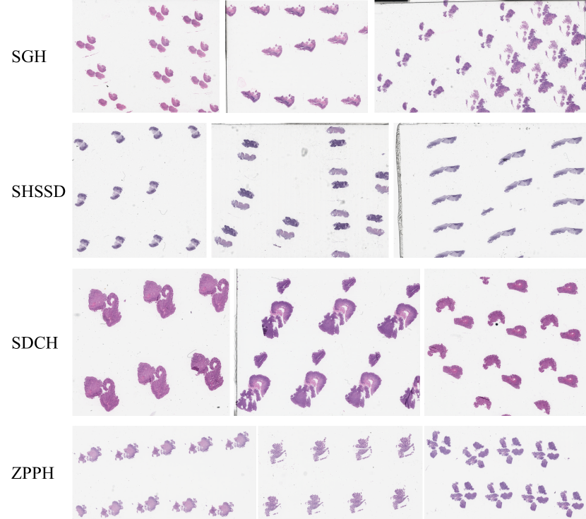
Figure 8: WSI examples from four institutes.

	Year	Sensitivity	Specificity
SGH	2015	1.0000	0.7753
	2018	0.9967	0.7995
	2019	1.0000	0.7829
SHSSD		1.0000	0.7371
SDCH		1.0000	0.6571
ZPPH		1.0000	0.7527

Table 3: Screening results in real-world scenario.

We apply our best model on these data and present sensitivity, and specificity in Table. 3. We achieve the sensitivity of $100.00\%$ in $5$ testing set, $99.67\%$ in the other, and the specificity is around $75\%$ in most of the cases.

However, the data distribution in the real-world scenario is different from our training and validation dataset, i.e., less positive samples and more outliers such as out of focus samples.

Moreover, the procedures in slide preparation also cause the differences (shown in Figure. 8). The sectioned tissues of SDCH are thicker than others, and they are stained much darker, which lead to the lowest specificity. WSIs from SHSSD are more blueish than SGH. Besides SGH, ZPPH also uses the machines for automatic sectioning and staining, so the performance on ZPPH data is higher than the other two institutes.

6 Discussion of Failure Cases

6.1 Out of Focus Slides

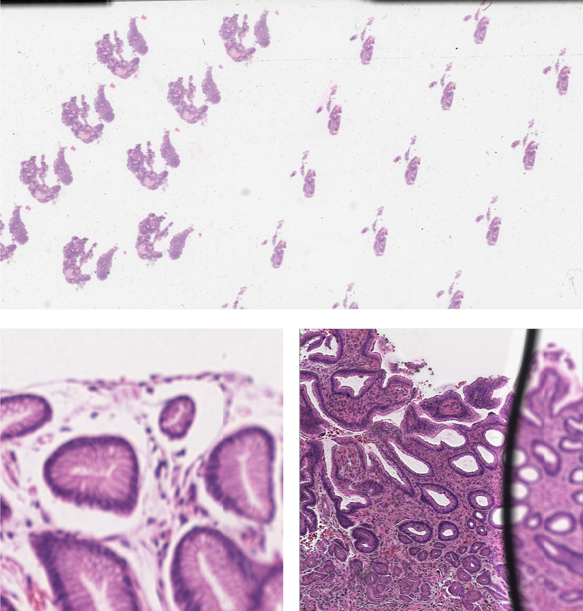
Figure 9: Top: an out of focus WSI. Left: a patch of the blurred image. Right: partially out of focus example.

As shown in Figure. 9, Our proposed model fails on these blurred images. The blurry is caused by out of focus during scanning. Instead of focusing on the tissue sections, the scanner focuses on the dust.

There is no effective way to classify the out of focus images correctly since they are highly blurred. So we add a blurry detection module, i.e., if it is a blurred image, there is no need to continue to classify whether it is positive or negative. We manually pick $1324$ blurred images (totally blurred and partially blurred) and $5512$ clear images to train a small neural network with $2$ $5\times 5$ convolution layers and a fully connected layer.

6.2 Failure Cases by Subtypes

Collaborating pathologists analyzed our testing results and found that errors are more from certain types of disease.

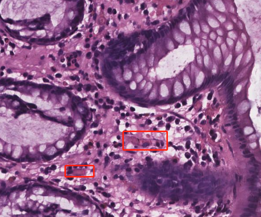
Figure 10: Signet ring cell carcinoma (signet ring cell in red bounding box).

Samples from signet ring cell carcinoma are easily missed since there are not many signet ring cells in the WSIs, and the size of cells is too small compare with the whole tissue. Even pathologists need further examination to diagnose (shown in Figure. 10).

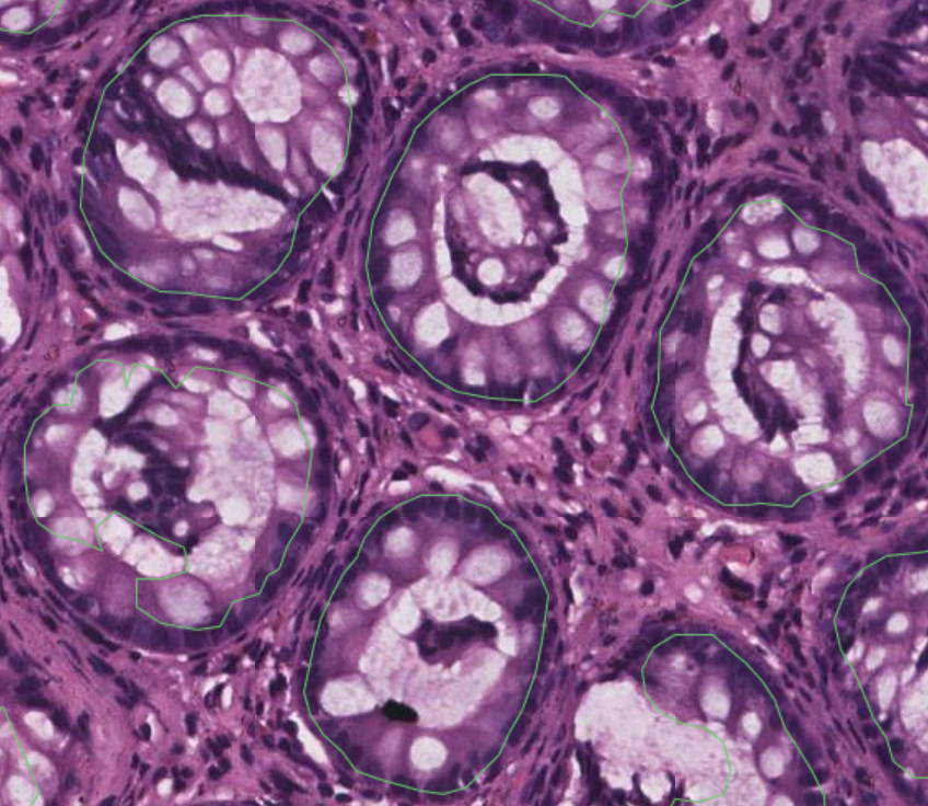
Figure 11: Intestinal metaplasia. Regions in the green contours are identified as cancer by the algorithm.

Some of intestinal metaplasia cases are classified as positive because intestinal metaplasia is a precancerous condition, i.e., “borderline” between positive and negative (shown in Figure. 11).

To solve this issue, we actively communicate with pathologists to get more of these types of samples to add to the training set and try to improve the performance of our algorithm on these subtypes.

7 Conclusion and Future Work

In conclusion, with the assumption that detailed lesion region annotation is necessary for the network to locate the crucial part in the gigapixel resolution WSIs and achieve the better performance, we designed a semi-automated annotation system and collected a large dataset consisting of $518$ WSIs with lesion region masks and over $10,000$ samples with screening results. To exploit our dataset, we propose a gastric slides screening framework to reduce the workload of pathologists and lower the inter-observer variability. The whole framework consists of three networks, a multi-task network for patch-level classification and segmentation, a 3-layer feed-forward network for slide-level screening result, and a simple segmentation network for foreground extraction.

One of the possible future direction of this project is cancer subtype diagnosis. Instead of just providing the “positive/negative” screening result, an automated lesion type diagnosis system could present the result like “adenocarcinoma”, “signet ring cell carcinoma”, “chronic atrophic gastritis”, etc. Furthermore, since a single WSI may contain multiple lesion types, displaying the labels on each segmented region/ROI could be more helpful, which requires an instance-level segmentation structure.

References

- Albarqouni et al. [2016] Albarqouni, S., Baur, C., Achilles, F., Belagiannis, V., Demirci, S., Navab, N., 2016. Aggnet: deep learning from crowds for mitosis detection in breast cancer histology images. IEEE transactions on medical imaging 35, 1313–1321.
- Barker et al. [2016] Barker, J., Hoogi, A., Depeursinge, A., Rubin, D.L., 2016. Automated classification of brain tumor type in whole-slide digital pathology images using local representative tiles. Medical image analysis 30, 60–71.
- Bray et al. [2018] Bray, F., Ferlay, J., Soerjomataram, I., Siegel, R.L., Torre, L.A., Jemal, A., 2018. Global cancer statistics 2018: Globocan estimates of incidence and mortality worldwide for 36 cancers in 185 countries. CA: a cancer journal for clinicians 68, 394–424.
- Chen et al. [2017] Chen, H., Qi, X., Yu, L., Dou, Q., Qin, J., Heng, P.A., 2017. Dcan: Deep contour-aware networks for object instance segmentation from histology images. Medical image analysis 36, 135–146.
- Chen et al. [2018] Chen, L.C., Zhu, Y., Papandreou, G., Schroff, F., Adam, H., 2018. Encoder-decoder with atrous separable convolution for semantic image segmentation, in: Proceedings of the European conference on computer vision (ECCV), pp. 801–818.
- Cosatto et al. [2013] Cosatto, E., Laquerre, P.F., Malon, C., Graf, H.P., Saito, A., Kiyuna, T., Marugame, A., Kamijo, K., 2013. Automated gastric cancer diagnosis on h&e-stained sections; ltraining a classifier on a large scale with multiple instance machine learning, in: Medical Imaging 2013: Digital Pathology, International Society for Optics and Photonics. p. 867605.
- Coudray et al. [2018] Coudray, N., Ocampo, P.S., Sakellaropoulos, T., Narula, N., Snuderl, M., Fenyö, D., Moreira, A.L., Razavian, N., Tsirigos, A., 2018. Classification and mutation prediction from non–small cell lung cancer histopathology images using deep learning. Nature medicine 24, 1559.
- Dai et al. [2017] Dai, J., Qi, H., Xiong, Y., Li, Y., Zhang, G., Hu, H., Wei, Y., 2017. Deformable convolutional networks, in: Proceedings of the IEEE international conference on computer vision, pp. 764–773.
- Dong et al. [2018] Dong, N., Kampffmeyer, M., Liang, X., Wang, Z., Dai, W., Xing, E., 2018. Reinforced auto-zoom net: Towards accurate and fast breast cancer segmentation in whole-slide images, in: Deep Learning in Medical Image Analysis and Multimodal Learning for Clinical Decision Support. Springer, pp. 317–325.
- Duan et al. [2020] Duan, Q., Wang, G., Wang, R., Fu, C., Li, X., Gong, M., Liu, X., Xia, Q., Huang, X., Hu, Z., et al., 2020. Sensecare: A research platform for medical image informatics and interactive 3d visualization. arXiv preprint arXiv:2004.07031 .
- Fakhry et al. [2016] Fakhry, A., Zeng, T., Ji, S., 2016. Residual deconvolutional networks for brain electron microscopy image segmentation. IEEE transactions on medical imaging 36, 447–456.
- Gao et al. [2019] Gao, S.H., Cheng, M.M., Zhao, K., Zhang, X.Y., Yang, M.H., Torr, P., 2019. Res2net: A new multi-scale backbone architecture. arXiv preprint arXiv:1904.01169 .
- He et al. [2017] He, K., Gkioxari, G., Dollár, P., Girshick, R., 2017. Mask r-cnn, in: Proceedings of the IEEE international conference on computer vision, pp. 2961–2969.
- He et al. [2016] He, K., Zhang, X., Ren, S., Sun, J., 2016. Deep residual learning for image recognition, in: Proceedings of the IEEE conference on computer vision and pattern recognition, pp. 770–778.
- Hou et al. [2016] Hou, L., Samaras, D., Kurc, T.M., Gao, Y., Davis, J.E., Saltz, J.H., 2016. Patch-based convolutional neural network for whole slide tissue image classification, in: Proceedings of the IEEE Conference on Computer Vision and Pattern Recognition, pp. 2424–2433.
- Hu et al. [2018] Hu, B., Tang, Y., Eric, I., Chang, C., Fan, Y., Lai, M., Xu, Y., 2018. Unsupervised learning for cell-level visual representation in histopathology images with generative adversarial networks. IEEE journal of biomedical and health informatics 23, 1316–1328.
- Huang et al. [2017] Huang, G., Liu, Z., Van Der Maaten, L., Weinberger, K.Q., 2017. Densely connected convolutional networks, in: Proceedings of the IEEE conference on computer vision and pattern recognition, pp. 4700–4708.
- Krizhevsky et al. [2012] Krizhevsky, A., Sutskever, I., Hinton, G.E., 2012. Imagenet classification with deep convolutional neural networks, in: Advances in neural information processing systems, pp. 1097–1105.
- Van der Laak et al. [2000] Van der Laak, J.A., Pahlplatz, M.M., Hanselaar, A.G., de Wilde, P.C., 2000. Hue-saturation-density (hsd) model for stain recognition in digital images from transmitted light microscopy. Cytometry: The Journal of the International Society for Analytical Cytology 39, 275–284.
- Li et al. [2019a] Li, J., Hu, Z., Yang, S., 2019a. Accurate nuclear segmentation with center vector encoding, in: Chung, A.C.S., Gee, J.C., Yushkevich, P.A., Bao, S. (Eds.), Information Processing in Medical Imaging, Springer International Publishing, Cham. pp. 394–404.
- Li et al. [2019b] Li, J., Yang, S., Huang, X., Da, Q., Yang, X., Hu, Z., Duan, Q., Wang, C., Li, H., 2019b. Signet ring cell detection with a semi-supervised learning framework, in: Information Processing in Medical Imaging.
- Li et al. [2018a] Li, Y., Li, X., Xie, X., Shen, L., 2018a. Deep learning based gastric cancer identification, in: 2018 IEEE 15th International Symposium on Biomedical Imaging (ISBI 2018), IEEE. pp. 182–185.
- Li et al. [2018b] Li, Z., Zhang, X., Müller, H., Zhang, S., 2018b. Large-scale retrieval for medical image analytics: A comprehensive review. Medical image analysis 43, 66–84.
- Lin et al. [2018] Lin, H., Chen, H., Dou, Q., Wang, L., Qin, J., Heng, P.A., 2018. Scannet: A fast and dense scanning framework for metastastic breast cancer detection from whole-slide image, in: 2018 IEEE Winter Conference on Applications of Computer Vision (WACV), IEEE. pp. 539–546.
- Lin et al. [2017] Lin, T.Y., Goyal, P., Girshick, R., He, K., Dollár, P., 2017. Focal loss for dense object detection, in: Proceedings of the IEEE international conference on computer vision, pp. 2980–2988.
- Liu et al. [2017] Liu, Y., Gadepalli, K., Norouzi, M., Dahl, G.E., Kohlberger, T., Boyko, A., Venugopalan, S., Timofeev, A., Nelson, P.Q., Corrado, G.S., et al., 2017. Detecting cancer metastases on gigapixel pathology images. arXiv preprint arXiv:1703.02442 .
- Long et al. [2015] Long, J., Shelhamer, E., Darrell, T., 2015. Fully convolutional networks for semantic segmentation, in: Proceedings of the IEEE conference on computer vision and pattern recognition, pp. 3431–3440.
- Mercan et al. [2017] Mercan, C., Aksoy, S., Mercan, E., Shapiro, L.G., Weaver, D.L., Elmore, J.G., 2017. Multi-instance multi-label learning for multi-class classification of whole slide breast histopathology images. IEEE transactions on medical imaging 37, 316–325.
- Oikawa et al. [2017] Oikawa, K., Saito, A., Kiyuna, T., Graf, H.P., Cosatto, E., Kuroda, M., 2017. Pathological diagnosis of gastric cancers with a novel computerized analysis system. Journal of pathology informatics 8.
- Otsu [1979] Otsu, N., 1979. A threshold selection method from gray-level histograms. IEEE transactions on systems, man, and cybernetics 9, 62–66.
- Qaiser et al. [2019] Qaiser, T., Tsang, Y.W., Taniyama, D., Sakamoto, N., Nakane, K., Epstein, D., Rajpoot, N., 2019. Fast and accurate tumor segmentation of histology images using persistent homology and deep convolutional features. Medical image analysis 55, 1–14.
- Redmon and Farhadi [2018] Redmon, J., Farhadi, A., 2018. Yolov3: An incremental improvement. arXiv preprint arXiv:1804.02767 .
- Ronneberger et al. [2015] Ronneberger, O., Fischer, P., Brox, T., 2015. U-net: Convolutional networks for biomedical image segmentation, in: International Conference on Medical image computing and computer-assisted intervention, Springer. pp. 234–241.
- Rota Bulò et al. [2018] Rota Bulò, S., Porzi, L., Kontschieder, P., 2018. In-place activated batchnorm for memory-optimized training of dnns, in: Proceedings of the IEEE Conference on Computer Vision and Pattern Recognition, pp. 5639–5647.
- Ruifrok et al. [2001] Ruifrok, A.C., Johnston, D.A., et al., 2001. Quantification of histochemical staining by color deconvolution. Analytical and quantitative cytology and histology 23, 291–299.
- Su et al. [2015] Su, H., Liu, F., Xie, Y., Xing, F., Meyyappan, S., Yang, L., 2015. Region segmentation in histopathological breast cancer images using deep convolutional neural network, in: 2015 IEEE 12th International Symposium on Biomedical Imaging (ISBI), IEEE. pp. 55–58.
- Szegedy et al. [2016] Szegedy, C., Vanhoucke, V., Ioffe, S., Shlens, J., Wojna, Z., 2016. Rethinking the inception architecture for computer vision, in: Proceedings of the IEEE conference on computer vision and pattern recognition, pp. 2818–2826.
- Tan and Le [2019] Tan, M., Le, Q.V., 2019. Efficientnet: Rethinking model scaling for convolutional neural networks. arXiv preprint arXiv:1905.11946 .
- Xu et al. [2015] Xu, J., Xiang, L., Liu, Q., Gilmore, H., Wu, J., Tang, J., Madabhushi, A., 2015. Stacked sparse autoencoder (ssae) for nuclei detection on breast cancer histopathology images. IEEE transactions on medical imaging 35, 119–130.
- Yoshida et al. [2018] Yoshida, H., Shimazu, T., Kiyuna, T., Marugame, A., Yamashita, Y., Cosatto, E., Taniguchi, H., Sekine, S., Ochiai, A., 2018. Automated histological classification of whole-slide images of gastric biopsy specimens. Gastric Cancer 21, 249–257.
- Yu et al. [2018] Yu, F., Wang, D., Shelhamer, E., Darrell, T., 2018. Deep layer aggregation, in: Proceedings of the IEEE Conference on Computer Vision and Pattern Recognition, pp. 2403–2412.
- Zhang et al. [2015a] Zhang, X., Dou, H., Ju, T., Xu, J., Zhang, S., 2015a. Fusing heterogeneous features from stacked sparse autoencoder for histopathological image analysis. IEEE journal of biomedical and health informatics 20, 1377–1383.
- Zhang et al. [2014] Zhang, X., Liu, W., Dundar, M., Badve, S., Zhang, S., 2014. Towards large-scale histopathological image analysis: Hashing-based image retrieval. IEEE Transactions on Medical Imaging 34, 496–506.
- Zhang et al. [2015b] Zhang, X., Xing, F., Su, H., Yang, L., Zhang, S., 2015b. High-throughput histopathological image analysis via robust cell segmentation and hashing. Medical image analysis 26, 306–315.
- Zhang et al. [2019] Zhang, Z., Chen, P., McGough, M., Xing, F., Wang, C., Bui, M., Xie, Y., Sapkota, M., Cui, L., Dhillon, J., et al., 2019. Pathologist-level interpretable whole-slide cancer diagnosis with deep learning. Nature Machine Intelligence 1, 236.
- Zhu et al. [2017] Zhu, X., Yao, J., Zhu, F., Huang, J., 2017. Wsisa: Making survival prediction from whole slide histopathological images, in: Proceedings of the IEEE Conference on Computer Vision and Pattern Recognition, pp. 7234–7242.