Modeling of Dynamical Systems via Successive Graph Approximations

Abstract

In this work, we propose a non-parametric technique for online modeling of systems with unknown nonlinear Lipschitz dynamics. The key idea is to successively utilize measurements to approximate the graph of the state-update function using envelopes described by quadratic constraints. The proposed approach is then demonstrated on two control applications: $(i)$ computation of tractable bounds for un-modelled dynamics, and $(ii)$ computation of positive invariant sets. We further highlight the efficacy of the proposed approach via a detailed numerical example.

I Introduction

Characterization of system model and associated uncertainties is of paramount importance while dealing with autonomous systems. In recent times, as data-driven decision making and control becomes ubiquitous [1, 2], system identification methods are being integrated with control algorithms for control of uncertain dynamical systems. In computer science community, data driven reinforcement learning algorithms [3, 4] have been extensively utilized for policy and value function learning of uncertain systems. In control theory, if the actual model of a system is unknown, adaptive control [5, 6] strategies have been applied for simultaneous system identification and control. Techniques for system modelling and identification have been traditionally rooted in statistics and data sciences [7, 8]. Statistical models that describe observed data, can be classified into parametric [9], non-parametric and semi-parametric [10] models.

Parametric models assume a model structure a priori, based on the application and domain expertise of the designer. In almost all of classical adaptive control methods, parametric models are learned from data in terms of point estimates, and asymptotic convergence of such estimates are proven under persistence of excitation [11] conditions. The concept of online model learning and adaptation has been extended to systems under constraints as well, after obtaining a set or a confidence interval containing possible realizations of the system model. Gaussian Mixture Modeling (GMM) [12, 13] has also been used to identify unknown system parameters, via an expectation maximization algorithm.

However, parametric models are restricted only to specified forms of function classes, and so to widen the richness of model estimates, non-parametric models are increasingly being utilized, whereby the model structure is also inferred from data. For non-parametric modeling of systems, Gaussian Process (GP) regression [14] has been one of the most widely used tools in control theory literature. GP regression keeps track of a Gaussian distribution over infinite dimensional function spaces, in terms of a mean function and a covariance kernel, which are updated with data. Given any system state, GP regression returns the mean function value at that state, along with a confidence interval. Kernel regression methods such as local linear regression [15, 16] and Nadaraya-Watson estimator [17] are some other non-parametric methods for system identification and control. Estimates obtained using these methods often come with confidence intervals as detailed in [18], instead of sets containing all possible realizations of the system, which is a critical drawback from the perspective of robust control.

The focus of this paper is to propose a simple non-parametric approach for modelling the unknown dynamics of a discrete time autonomous system. The proposed approach applies to unknown nonlinear systems with dynamics described by a state-update function that is globally Lipschitz over a bounded domain, with known Lipschitz constant. Instead of identifying the state-update function itself, we identify its graph- the set of all state and corresponding state-update function value pairs. This is done by computing envelopes of the state-update function, which are sets that contain the graph of the state-update function. These envelopes are built by using historical data of state trajectories and the Lipschitz property of the function.

The paper is divided into two parts. In the first part we describe a method to compute the envelope set which contains all possible realizations of the unknown state-update function at any given state. The authors in [19, 20] use GP regression modeling to provide probabilistic confidence intervals on the state-update function at any given state. The key difference is that we approximate a function via a subset of the Euclidean space rather than approximating it directly in a function space. In the second part, we provide two applications of the proposed approach, namely $(i)$ obtaining tractable set based outer approximations of the unknown state-update function and $(ii)$ computing positive invariant sets [21, 22] for the unknown system using the s-procedure [23].

II Notation

$\|\cdot\|$ denotes the Euclidean norm in $\mathbb{R}^{n}$ unless explicitly stated otherwise. An open ball in $\mathbb{R}^{n}$, of radius $r$ and centered at $x$ is denoted as $\mathcal{B}_{r}(x)$. Notation $O(\cdot)$ is used to describe an expression that decays to 0 as fast as its argument. The Minkowski sum of two sets $A$ and $B$ is given by

$$A\oplus B=\{a+b\ |a\in A,b\in B\}.$$

We use $\mathrm{ell}(c,R)$ to denote an ellipse that is centered at point $c$ and has a shape matrix $R=R^{\top}\succ 0$.

III Problem Formulation

Consider the discrete time autonomous, time invariant system

$$x_{k+1}=f(x_{k}),$$ (1)

where the state-update function $f(\cdot):\mathcal{X}\rightarrow\mathcal{X}$ describes the system dynamics and is defined over the state space $\mathcal{X}\subseteq\mathbb{R}^{n}$.

Assumption 1

The function $f(\cdot):\mathcal{X}\rightarrow\mathcal{X}$ is continuous and differentiable over a convex and closed domain $\mathcal{X}\subset\mathbb{R}^{n}$ with $\|\nabla f(x)\|\leq L$, for all $x\in\mathcal{X}$ and some $L>0$.

Proposition 1 ([24])

Let Assumption 1 hold. Then $\|f(x)-f(y)\|\leq L\|x-y\|$ for all $x,y\in\mathcal{X}$, i.e., $f(\cdot)$ is $L$-Lipschitz in the domain $\mathcal{X}$.

Now suppose that the function $f(\cdot)$ is unknown. The objective of this work is to compute a set containing $f(x)$ for any state $x$ in the state space $\mathcal{X}$ using trajectory data $\{x_{0},x_{1},x_{2},\dots\}$ and the Lipschitz property of the unknown function $f(\cdot)$.

Assumption 2

The Lipschitz constant $L$ is known.

In case the Lipschitz constant $L$ is unknown, it can be estimated using methods such as [25]. Integrating such estimation methods into the proposed work is a subject of future research.

Remark 1

The problem of characterizing $L-$Lipschitz un-modelled dynamics $d(\cdot)$ in

$$x_{k+1}=\underbrace{\bar{f}(x_{k})}_{\textnormal{assumed model}}+\underbrace{d(x_{k})}_{\textnormal{un-modelled dynamics}}$$

can also be cast into a problem of the form (1). In this case, we use the trajectory data $\{x_{0},x_{1},x_{2},\dots\}$ to construct $\{x_{1}-\bar{f}(x_{0}),x_{2}-\bar{f}(x_{1}),\dots\}$ which is then used for computing a set containing $d(x)$ at $x\in\mathcal{X}$.

IV Proposed Approach

We will make use of the following definitions.

Definition 1 (Graph)

The graph of function $f(\cdot):\mathcal{X}\rightarrow\mathcal{X}$ is the set

$$G(f)=\{(x,f(x))\in\mathbb{R}^{n}\times\mathbb{R}^{n}|\ \forall x\in\mathcal{X}\}.$$ (2)

Definition 2 (Envelope)

An envelope of function $f(\cdot):\mathcal{X}\rightarrow\mathcal{X}$ is a set $\mathbf{E}^{f}\subseteq\mathbb{R}^{n}\times\mathbb{R}^{n}$, with the property

$$G(f)\subseteq\mathbf{E}^{f}.$$ (3)

We use trajectory data $\{x_{0},x_{1},x_{2},\dots\}$ of the system dynamics (1) to construct an envelope of the system dynamics $f(\cdot)$. Observe that the trajectory data can be used to construct tuples $(x_{k},f(x_{k}))=(x_{k},x_{k+1})$. In particular, at every time instant $N$, we have access to measurements $(x_{k},f(x_{k}))$, for all $k=0,1,\dots,N-1$. These measurements are utilized to construct envelopes recursively. Our approach for envelope construction is summarised as follows:

1. At time $N$, compute an envelope $\mathcal{E}(x_{N-1})$ using the tuple $(x_{N-1},f(x_{N-1}))$ and the $L-$Lipschitz property of $f(\cdot)$.

2. Compute a refined envelope $\mathbf{E}^{f}_{N}$ by intersecting the envelope $\mathbf{E}^{f}_{N-1}$ from time $N-1$ with the envelope $\mathcal{E}(x_{N-1})$ computed in step 1), i.e.,

   $$\mathbf{E}^{f}_{N}=\mathbf{E}^{f}_{N-1}\cap\mathcal{E}(x_{N-1}).$$

For 1), the envelope is obtained as the sublevel set of a quadratic function. Afterwards, 2) is obtained by using the set membership approach [26, 27, 28, 29]. Finally, we use the computed envelope for obtaining a set containing the value of $f(x)$ at any $x\in\mathcal{X}$, using the notion of a slice of an envelope defined below.

Definition 3 (Envelope Slice)

The slice of an envelope $\mathbf{E}^{f}\subseteq\mathbb{R}^{n}\times\mathbb{R}^{n}$ at a given $\bar{x}\in\mathcal{X}$ is the set defined as

$$\mathbf{E}^{f}\Big{|}_{x=\bar{x}}=\{(x,y)\in\mathbf{E}^{f}\subseteq\mathbb{R}^{n}\times\mathbb{R}^{n}|x=\bar{x}\}.$$ (4)

Fig. 1 shows a typical realization of the proposed approach along with the associated set definitions which are detailed next.

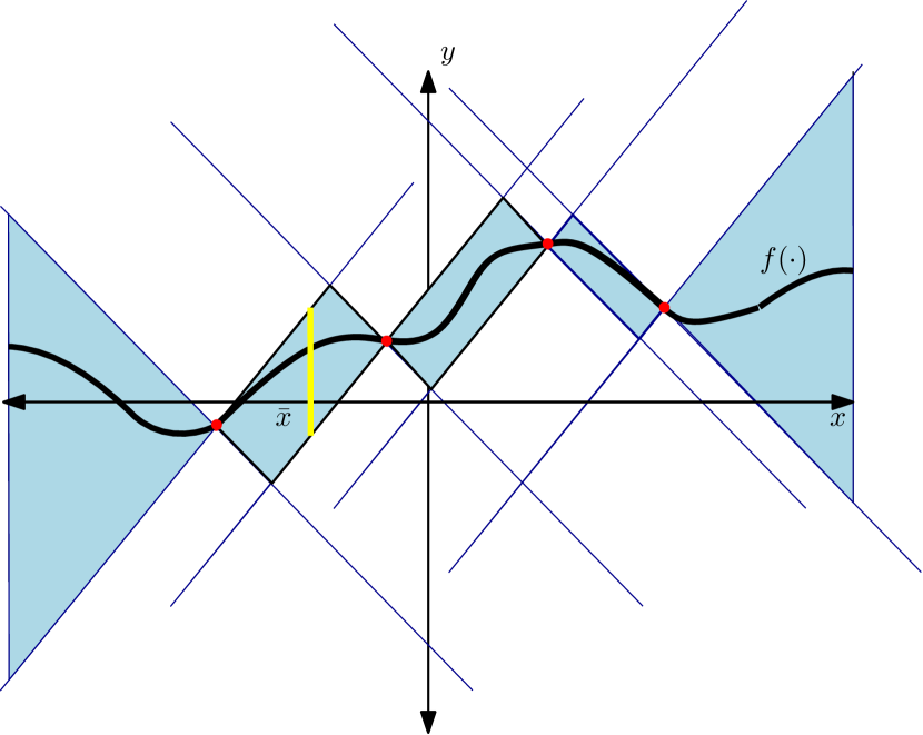
Figure 1: Construction of an envelope for a one dimensional system to approximate the graph $G(f)$ (black curve) of its state-update function $f(\cdot)$. Tuples $(x,f(x))$ (red points) obtained from trajectory data are used for constructing the envelope (blue set) and its slice (yellow set) at $x=\bar{x}$.

IV-A Envelope Construction

Inspired by [30, 31], we use quadratic constraints (QCs) as our main tool to approximate the graph of a function. A definition appropriate for our purposes is presented below.

Definition 4 (QC Satisfaction)

A set $\mathbb{X}\subset\mathbb{R}^{n}$ satisfies the quadratic constraint specified by a symmetric matrix $Q$ if

$$\begin{bmatrix}x\\ 1\end{bmatrix}^{\top}Q\begin{bmatrix}x\\ 1\end{bmatrix}\leq 0,\quad\forall x\in\mathbb{X}.$$ (5)

The following proposition uses a QC to characterize a coarse approximation of the graph of an $L-$Lipschitz function.

Proposition 2

The graph $G(f)$ of an $L-$Lipschitz function $f(\cdot)$ satisfies the QC specified by the matrix

$$Q_{L}^{f}(x_{k})=\begin{bmatrix}-L^{2}\mathbb{I}_{n}&\mathbf{0}_{n\times n}&L^{2}x_{k}\\ \mathbf{0}_{n\times n}&\mathbb{I}_{n}&-f(x_{k})\\ L^{2}x_{k}^{\top}&-f^{\top}(x_{k})&-L^{2}x_{k}^{\top}x_{k}\\ &&\hskip 28.45274pt+f^{\top}(x_{k})f(x_{k})\end{bmatrix},$$ (6)

for any $(x_{k},f(x_{k}))\in G(f)$.

Proof:

Using the definition of the $L-$Lipschitz property of $f(\cdot)$ (from Proposition 1), at any $(x_{k},f(x_{k}))\in G(f)$, we have

$$\|f(x)-f(x_{k})\|\leq L\|x-x_{k}\|\quad~{}~{}~{}\forall(x,f(x))\in G(f),$$

$$\iff (f(x)-f(x_{k}))^{\top}(f(x)-f(x_{k}))\leq L^{2}(x-x_{k})^{\top}(x-x_{k})$$

$$~{}~{}~{}~{}~{}~{}~{}~{}~{}~{}~{}~{}~{}~{}~{}~{}~{}~{}~{}~{}~{}~{}~{}~{}~{}~{}~{}~{}~{}~{}~{}~{}~{}~{}~{}~{}~{}~{}~{}~{}~{}~{}\forall(x,f(x))\in G(f),$$

$$\iff \begin{bmatrix}x\\ f(x)\\ 1\end{bmatrix}^{\top}Q_{L}^{f}(x_{k})\begin{bmatrix}x\\ f(x)\\ 1\end{bmatrix}\leq 0,\quad\forall(x,f(x))\in G(f).$$

Therefore $G(f)$ satisfies the QC specified by $Q_{L}^{f}(x_{k})$. ∎

The following corollary then gives us the definition of the envelope $\mathcal{E}(x_{k})$.

Corollary 1

The set defined by

$$\mathcal{E}(x_{k})=\{(x,y)\in\mathbb{R}^{n}\times\mathbb{R}^{n}|\begin{bmatrix}x\\ y\\ 1\end{bmatrix}^{\top}Q_{L}^{f}(x_{k})\begin{bmatrix}x\\ y\\ 1\end{bmatrix}\leq 0\}$$ (7)

is an envelope for all $L-$Lipschitz functions that pass through $(x_{k},f(x_{k}))$.

Proof:

Let $g(\cdot)$ be any $L-$ Lipschitz function such that $g(x_{k})=f(x_{k})$. From the definition of Lipschitz property we have

$$\|g(x)-f(x_{k})\|\leq L\|x-x_{k}\|,\quad\forall(x,g(x))\in G(g),$$

$$\iff \begin{bmatrix}x\\ g(x)\\ 1\end{bmatrix}^{\top}Q_{L}^{f}(x_{k})\begin{bmatrix}x\\ g(x)\\ 1\end{bmatrix}\leq 0,\quad\forall(x,g(x))\in G(g),$$

$$\iff (x,g(x))\in\mathcal{E}(x_{k}),\quad\forall(x,g(x))\in G(g),$$

$$\iff G(g)\subseteq\mathcal{E}(x_{k}).\normalsize$$

∎

Remark 2

The proposed formulation can also be extended to accommodate bounded noise in the measurements of $x_{k}$ in (1). Suppose that the measurement model is given by

$$z_{k}=x_{k}+w_{k},$$

where $w_{k}$ belongs to a compact set $\mathcal{W}$. Then the envelope that is guaranteed to contain $G(f)$ is given by $\mathcal{E}(z_{k})\oplus(\mathcal{W}\times\mathcal{W})$ where $Q_{L}^{f}(\cdot)$ is now constructed using $(z_{k},z_{k+1})$.

IV-B Successive Graph Approximation

At time $N$, the envelope $\mathcal{E}(x_{N-1}))$ constructed in (7) using the tuple $(x_{N-1},f(x_{N-1}))$ can now be used to recursively compute a new envelope $\mathbf{E}^{f}_{N}$ by refining the envelope $\mathbf{E}^{f}_{N-1}$ from time $N-1$ via set intersection-

$$\mathbf{E}^{f}_{N}=\mathbf{E}^{f}_{N-1}\cap\mathcal{E}(x_{N-1})$$ (8)

In the following lemma we show that the sets computed in this fashion are indeed envelopes.

Lemma 1

For $N\geq 1$, given a sequence $\{x_{k}\}_{k=0}^{N-1}$ obtained under the dynamics (1), we have

$$G(f)\subseteq\mathbf{E}^{f}_{N}=\mathbf{E}^{f}_{N-1}\cap\mathcal{E}(x_{N-1})=\bigcap_{k=0}^{N-1}\mathcal{E}(x_{k}).$$ (9)

Proof:

See Appendix. ∎

The recursion is initialized with the trivial envelope $\mathbf{E}^{f}_{0}=\mathbb{R}^{n}\times\mathbb{R}^{n}$. The procedure is described in Algorithm 1.

1

Initialization: $\mathbf{E}_{0}^{f}=\mathbb{R}^{n}\times\mathbb{R}^{n}$

2

Input: At time $N$, $(x_{N-1},f(x_{N-1}))$ and $\mathbf{E}^{f}_{N-1}$

Output: Approximation of $G(f)$ at time $N$: $\mathbf{E}^{f}_{N}$

3

4Compute $Q_{L}^{f}(x_{N-1})$ (from (6))

5 Compute $\mathcal{E}(x_{N-1})$ using $Q_{L}^{f}(x_{N-1})$ (from (7))

Set $\mathbf{E}^{f}_{N}=\mathbf{E}^{f}_{N-1}\cap\mathcal{E}(x_{N-1})$

Algorithm 1 Recursive Envelope Refinement

Note that since the envelope at any time $N$ is computed by intersecting with the envelope at time $N-1$, they are getting successively refined, i.e.,

$$\mathbf{E}^{f}_{N}\subseteq\mathbf{E}^{f}_{N-1}\subseteq\mathbf{E}^{f}_{N-2}\dots\subseteq\mathbf{E}^{f}_{0}$$ (10)

Now we provide a condition under which the shrinking sets generated by recursion (8) stop shrinking i.e., recursion (8) attains a fixed point. Intuitively, we would expect this to happen when the incoming tuples $(x,f(x))$ constructed from trajectory data have already been seen previously. The following definition formalises the notion of such trajectories.

Definition 5 (Periodic Orbit [32])

A $p$-periodic orbit of the discrete dynamical system (1) is the set of states obtained under dynamics $x_{k+1}=f(x_{k})$ with the property that $x_{k}=x_{k+p}$ for some finite $p\geq 1$ and for all $k\geq 0$, i.e.,

$$\mathcal{O}_{p}(x_{0}) =\{x\in\mathcal{X}\ |\ x_{k+1}=f(x_{k}),x_{k}=x_{k+p},$$

$$~{}~{}~{}~{}~{}~{}~{}~{}~{}~{}~{}~{}~{}~{}~{}~{}~{}~{}~{}~{}~{}~{}~{}~{}~{}~{}~{}~{}x=x_{k},\forall k\geq 0\}.$$ (11)

Note that the set $\mathcal{O}_{p}(\bar{x}_{\textnormal{eq}})=\{\bar{x}_{\textnormal{eq}}\}$ for all $p\geq 1$ where $\bar{x}_{\textnormal{eq}}$ is the fixed point $\bar{x}_{\textnormal{eq}}=f(\bar{x}_{\textnormal{eq}})$ of system (1). Associated to each fixed point, one can define the set of states that converge to it as follows.

Definition 6 (Domain of Attraction [33])

The domain of attraction of fixed point $\bar{x}_{\textnormal{eq}}$ is defined as the set

$$\mathbf{D}(\bar{x}_{\textnormal{eq}})=\{x\in\mathcal{X}|x_{k+1}=f(x_{k}),\lim_{k\rightarrow\infty}x_{k}=\bar{x}_{\textnormal{eq}},x=x_{0}\}.$$

The following proposition uses Definition 5 and Definition 6 to identify sufficient conditions on system trajectories for termination of the recursion (8).

Proposition 3

Given a system trajectory denoted by the set $\{x_{0},x_{1},x_{2},\dots\}$, the recursion (8) has a fixed point if either of the following conditions hold:

1. $\mathcal{O}_{p}(x_{k})\subseteq\{x_{0},x_{1},x_{2},\dots\}$ for some finite $p\geq 1$ and some $k\geq 0$.

2. $x_{0}\in\mathbf{D}(\bar{x}_{\textnormal{eq}})$ for some fixed point $\bar{x}_{\textnormal{eq}}$.

Proof:

See Appendix. ∎

Next we present how the envelope slice is derived from the constructed envelopes for obtaining a set-valued estimate of $f(x)$ at any $x\in\mathcal{X}$

IV-C Envelope Slice Computation

The set of possible values of function $f(\bar{x})$ at any $\bar{x}\in\mathcal{X}$ can be obtained using (7) from the function values $f(x_{k})$ collected at $k=\{0,1,2,\dots,N-1\}$. From only the $k$-th measurement, we can obtain an estimate of the set of possible values of $f(\bar{x})$, by constructing the slice of envelope $\mathcal{E}(x_{k})$ at $x=\bar{x}$, from Definition 3. We denote this slice with the set $\mathcal{S}(x_{k},\bar{x})$ as

$$\mathcal{S}(x_{k},\bar{x}) =\mathcal{E}(x_{k})\Big{|}_{x=\bar{x}},$$

$$=\{y\in\mathcal{X}|\begin{bmatrix}\bar{x}\\ y\\ 1\end{bmatrix}^{\top}Q^{f}_{L}(x_{k})\begin{bmatrix}\bar{x}\\ y\\ 1\end{bmatrix}\leq 0\}$$

$$=\{y\in\mathcal{X}|\begin{bmatrix}y\\ 1\end{bmatrix}^{\top}\bar{A}(k,\bar{x})\begin{bmatrix}y\\ 1\end{bmatrix}\leq 0\},$$ (12)

where we have denoted $\bar{A}(k,\bar{x})=MQ^{f}_{L}(x_{k})M^{\top}-L^{2}\begin{bmatrix}0&0\\ 0&(\bar{x}-2x_{k})^{\top}\bar{x}\end{bmatrix}$, for any $k=\{0,1,2,\dots,N-1\}$, with matrix $M=\begin{bmatrix}0&1&0\\ 0&0&1\end{bmatrix}$. Corollary 1 then implies $f(x)\in\mathcal{S}(x_{k},x)$ at any $x\in\mathcal{X}$.

Proposition 4

At any $\bar{x}\in\mathcal{X}$, $\mathcal{S}(x_{k},\bar{x})$ is a closed norm ball of radius $L\|\bar{x}-x_{k}\|$, centered at $f(x_{k})$ for each $k=\{0,1,\dots,N-1\}$.

Proof:

Expanding out (IV-C) gives us

$$\|f(\bar{x})-f(x_{k})\|^{2}\leq L^{2}\|\bar{x}-x_{k}\|^{2},$$ (13)

for each $k=\{0,1,\dots,N-1\}$ and thus proves the claim. ∎

As we successively collect data points $(x_{k},f(x_{k}))$ for $k=\{0,1,2,\dots,N-1\}$ under dynamics (1), the set of possible values of $f(\bar{x})$ at any $\bar{x}\in\mathcal{X}$ is refined as

$$\mathcal{F}_{N}(\bar{x})=\bigcap_{k=0}^{N-1}\mathcal{S}(x_{k},\bar{x})=\bigcap_{k=0}^{N-1}\mathcal{E}(x_{k})\Big{|}_{x=\bar{x}}=\mathbf{E}_{N}^{f}\Big{|}_{x=\bar{x}},$$ (14)

with the guarantee $f(\bar{x})\in\mathcal{F}_{N}(\bar{x})$ at any given time $N\geq 1$. Notice that $\mathcal{F}_{N}(\bar{x})$ is a slice of envelope $\mathbf{E}^{f}_{N}$ at $x=\bar{x}$, as per Definition 3. We further note that $\mathcal{F}_{N}(\bar{x})$ in (14) is convex and compact, as it is an intersection of convex and compact sets (13).

So far we have seen that the envelopes generated by Algorithm 1 are getting successively refined (in (10)) and possibly stop improving (as noted in proposition 3). But given a trajectory that yields a terminating recursion (8), where in the state space $\mathcal{X}$ are the envelope slices “tight”? We use the notion of the diameter of a compact set ([24]) to quantify “tightness” or size of the envelope slice. In the following theorem, we show that if a trajectory starts in the domain of attraction $\mathbf{D}(\bar{x}_{\textnormal{eq}})$ of a fixed point $\bar{x}_{\textnormal{eq}}$ of (1), then the error in approximation of $G(f)$ by $\mathbf{E}^{f}_{N}$ at points arbitrarily close to $\bar{x}_{\textnormal{eq}}$ (measured by the diameter of the envelope slice $\mathcal{F}_{N}(x)$ at any $x\in\mathcal{X}$), gets arbitrarily small for large enough $N$.

Theorem 1

Suppose we are given a system trajectory denoted by the set $\{x_{0},x_{1},x_{2},\dots,x_{N}\}$ where $x_{0}\in\mathbf{D}(\bar{x}_{\textnormal{eq}})$. Then for states $x$ arbitrarily close to $\bar{x}_{\textnormal{eq}}$, the diameter of $\mathcal{F}_{N}(x)$ is arbitrarily small for large enough $N$, i.e.,

$$\forall\epsilon>0,\exists~{}\bar{N}(\epsilon):$$

$$\max_{y\in\mathcal{F}_{N}(x)}\|y-f(x)\|=O(\epsilon),$$

$$\forall x\in\mathcal{B}_{\epsilon}(\bar{x}_{\textnormal{eq}}),\ \forall N\geq\bar{N}(\epsilon).$$

Proof:

See Appendix. ∎

V Applications

In this section we demonstrate two applications and corresponding computationally tractable algorithms that utilize the proposed approach in the paper.

V-A Ellipsoidal Outer Approximation of $\mathcal{F}_{N}(\bar{x})$

In order to design computationally tractable robust optimization [34] algorithms for all realizations of $f(x)$ at any $x\in\mathcal{X}$ and $N\geq 1$, one must have a “nice” geometric representation of the envelope slice $\mathcal{F}_{N}(\bar{x})=\mathbf{E}^{f}_{N}\Big{|}_{x=\bar{x}}$, for all $N\geq 1$. We hereby propose an approach to obtain an ellipsoidal outer approximation to $\mathcal{F}_{N}(\bar{x})$ for any $N\geq 1$ using the s-procedure [35, Section 11.4], having collected measurements at $k=0,1,\dots,N-1$,

Let us parametrize an ellipsoidal outer approximation of $\mathcal{F}_{N}(x_{N})$, which we denote by ell($c(\bar{x}),R(\bar{x})$) as

$$\textnormal{ell}(c(\bar{x}),R(\bar{x}))=$$

$$\{y\in\mathbb{R}^{n}|\ (y-c(\bar{x}))^{\top}R^{-1}(\bar{x})(y-c(\bar{x}))\leq 1\},$$

where vector $c(\bar{x})$ and matrix $R(\bar{x})$ are the decision variables, and are functions of $\bar{x}$. We seek the smallest ellipsoidal set such that

$$\mathcal{F}_{N}(\bar{x})=\bigcap_{k=0}^{N-1}\mathcal{S}_{k}(x_{k},\bar{x})\subseteq\textnormal{ell}(c(\bar{x}),R(\bar{x})).$$

From s-procedure [36] we know that the above holds true, if there exists scalars $\{\tau_{0},\tau_{1},\dots,\tau_{N-1}\}\geq 0$ such that

$$\begin{bmatrix}R^{-1}(\bar{x})&-R^{-1}(\bar{x})c(\bar{x})\\ -c^{\top}(\bar{x})R^{-1}(\bar{x})&c^{\top}(\bar{x})R^{-1}(\bar{x})c(\bar{x})\\ &\hskip 85.35826pt-1\end{bmatrix}$$

$$~{}~{}~{}~{}~{}~{}~{}~{}~{}~{}~{}~{}~{}~{}~{}~{}~{}~{}~{}~{}~{}~{}~{}~{}~{}~{}~{}~{}~{}~{}~{}~{}~{}~{}~{}~{}~{}-\sum\limits_{k=0}^{N-1}\tau_{k}\bar{A}^{s}(k,{\bar{x}})\preceq 0.$$ (15)

We reformulate the above feasibility problem (V-A) as a semi-definite program (SDP) in the appendix.

V-B Positive Invariant Set Computation

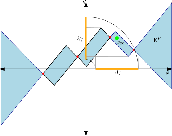
Figure 2: Illustration of invariance using an envelope of system dynamics. $\mathcal{X}_{I}$(orange) is invariant for all $f(\cdot)$ with $G(f)\subset\mathbf{E}^{f}$(blue).

Definition 7 (Positive Invariant Set)

A set $\mathcal{X}_{I}\subseteq\mathcal{X}$ is said to be positive invariant for the system with dynamics (1) if

$$x\in\mathcal{X}_{I}\Rightarrow f(x)\in\mathcal{X}_{I},$$

i.e. the set $\mathcal{X}_{I}$ maps to itself, under the dynamics map $f(\cdot):\mathcal{X}\rightarrow\mathcal{X}$.

Let there be an equilibrium point $\bar{x}_{\textnormal{eq}}$ defined as $f(\bar{x}_{\textnormal{eq}})=\bar{x}_{\textnormal{eq}}$. We wish to characterize a positive invariant set $\mathcal{X}_{I}\subseteq\mathcal{X}$ containing this equilibrium. For the sake of computational tractability, we represent this set as an intersection of $n_{I}$ ellipsoids, centered at $\bar{x}_{\textnormal{eq}}$. We parameterize the invariant set for some $P_{j}\succ 0$ with $j=1,2,\dots n_{I}$ as follows

$$\mathcal{X}_{I}=\{x\in\mathbb{R}^{n}| \ \begin{bmatrix}x\\ 1\end{bmatrix}^{\top}\begin{bmatrix}P_{j}&-P_{j}\bar{x}_{\textnormal{eq}}\\ -\bar{x}^{\top}_{\textnormal{eq}}P_{j}&\bar{x}^{\top}_{\textnormal{eq}}P_{j}\bar{x}_{\textnormal{eq}}-1\end{bmatrix}\begin{bmatrix}x\\ 1\end{bmatrix}\leq 0,\$$

$$~{}~{}~{}~{}~{}~{}~{}~{}~{}~{}~{}~{}~{}~{}~{}~{}~{}~{}~{}~{}~{}~{}~{}~{}~{}~{}~{}~{}~{}\forall j=1,2,\dots n_{I}\}.$$ (16)

Observing that the tuple $(x,f(x))\in G(f)\subseteq\mathbf{E}^{f}_{N}$ consists of a point $x\in\mathcal{X}$ and its image $f(x)\in\mathcal{X}$ under the map $f(\cdot)$, we can use the collected $Q_{L}^{f}(x_{k})$’s for $k=\{0,1,\dots,N-1\}$ at any time $N$, to obtain a sufficiency condition for (V-B) as detailed in the following proposition.

Proposition 5

Suppose that we are given an approximation of $G(f)$ at time $N$, i.e., $\mathbf{E}^{f}_{N}=\bigcap_{k=0}^{N-1}\mathcal{E}(x_{k})$, constructed by Algorithm 1. If there exists $\tau_{k}\geq 0$, for all $k=0,1,\dots N-1$ and $P_{j}\succ 0$, $\rho_{jm}>0$ for all $j,m=1,2,\dots,n_{I}$, such that the following Bilinear Matrix Inequality (BMI) is feasible

$$\sum_{j=1}^{n_{I}} \begin{bmatrix}-\rho_{jm}P_{j}&0&\rho_{jm}P_{j}\bar{x}_{\textnormal{eq}}\\ 0&P_{m}&-P_{m}\bar{x}_{\textnormal{eq}}\\ \bar{x}^{\top}_{\textnormal{eq}}\rho_{jm}P_{j}&-\bar{x}^{\top}_{\textnormal{eq}}P_{m}&-\bar{x}^{\top}_{\textnormal{eq}}(\rho_{jm}P_{j}-P_{m})\bar{x}_{\textnormal{eq}}\\ &&\hskip 28.45274pt+(\rho_{jm}-1)\end{bmatrix}$$

$$~{}~{}~{}~{}~{}~{}~{}~{}~{}~{}~{}~{}~{}~{}~{}~{}~{}~{}~{}~{}~{}~{}~{}~{}~{}~{}~{}~{}~{}~{}~{}~{}-\sum\limits_{k=0}^{N-1}\tau_{k}Q_{L}^{f}(x_{k})\preceq 0,$$ (17)

for all $m=1,2,\dots,n_{I}$, then the set $\mathcal{X}_{I}$ is a positive invariant set for the system with dynamics (1).

Proof:

See Appendix. ∎

One of many approaches to solving such a BMI (see [37]) is detailed in the appendix.

VI Numerical Example

In this section we demonstrate the approach proposed in Section IV for characterizing the un-modelled dynamics of a pendulum. We also showcase construction of a positive invariant set for this system, utilizing the tools from Section V-B.

VI-A Pendulum Model

The continuous time model of the considered pendulum is given by

$$ml^{2}\ddot{\theta}+mgl\sin{\theta}+\tilde{d}(\theta,\dot{\theta})=\mathcal{T},$$ (18)

where $m$ is the mass, $l$ is the length, $\theta$ is the angle the pendulum makes with the vertical axis, $\tilde{d}(\theta,\dot{\theta})$ is an un-modelled damping force with known Lipschitz constant $L_{d}$ and $\mathcal{T}$ is a known external torque. In this work, we simulate the system with the damping force $\tilde{d}(\theta,\dot{\theta})=-L_{d}\dot{\theta}$ and characterize state-dependent bounds for the same. We write the pendulum dynamics (18) in state-space form as

$$\begin{bmatrix}\dot{\theta}\\ \ddot{\theta}\end{bmatrix}=\begin{bmatrix}0&I\\ 0&0\end{bmatrix}\begin{bmatrix}{\theta}\\ \dot{\theta}\end{bmatrix}+\begin{bmatrix}0\\ \frac{\mathcal{T}}{ml^{2}}-\frac{g}{l}\sin\theta-\frac{\tilde{d}(\theta,\dot{\theta})}{ml^{2}}\end{bmatrix},$$ (19)

where $x=[\theta~{}\dot{\theta}]^{\top}$ is the state of the pendulum. We consider a torque $\mathcal{T}$ that stabilizes the pendulum’s state when it’s upright, i.e., when $\bar{x}_{\mathrm{eq}}=[\pi~{}0]^{\top}$. We discretize system (19) and write it in the form of (1) as $x_{k+1}=f(x_{k})$. We then simulate the system forward in time with a variational integrator for mechanical systems, as in [38]. The simulation parameters are: $m=2\mathrm{kg},l=2\mathrm{m}$ and $L_{d}=0.2\mathrm{N}$.

VI-B Envelope Construction for Damping Force

The discrete time model $x_{k+1}=f(x_{k})$ is decomposed as

$$x_{k+1}=\underbrace{\bar{f}(x_{k})}_{\textnormal{assumed model}}+\underbrace{d(x_{k})}_{\textnormal{un-modelled damping}},$$ (20)

where $x_{k}=[\theta_{k}~{}\dot{\theta}_{k}]^{\top}$ , $d(\cdot)$ is the unknown damping in discrete time with Lipschitz constant $\tilde{L}_{d}=\frac{L_{d}T_{S}}{ml^{2}}$ and $T_{S}=0.005s$ is the sampling period. Our experiment is succinctly described below:

• Trajectories up to a specified time instant $N$, starting from four different initial conditions $x_{0}=\{[\frac{5\pi}{6}~{}0]^{\top},[\frac{5\pi}{3}~{}-0.5]^{\top},[\frac{\pi}{6}~{}0]^{\top},[\frac{5\pi}{4}~{}-0.2]^{\top}\}$ are simulated (solid lines in Fig. 3) and stored.

• Realizations of the un-modelled dynamics $d(x_{k})$ are recorded via the measurement model $d(x_{k})=x_{k+1}-\bar{F}(x_{k})$.

• Having recorded the measurements $(x_{k},d(x_{k}))$ for $k=0,1,\dots,N-1$ along all four trajectories, we construct the estimate $\mathcal{D}_{N}(\bar{x})$ (defined as in (14)) of $d(\bar{x})$ at six different query points ($\star$ and $\circ$ in Fig. 3) using Algorithm 1.

TABLE I: Uncertainty range (up to three significant digits). Symbol $[\cdot,\cdot]$ denotes an interval

Query Point $\bar{x}$	$\mathcal{D}_{100}(\bar{x})/10^{-4}$	$\mathcal{D}_{4000}(\bar{x})/10^{-4}$
$[2.12\ -0.45]^{\top}$	$[-0.837,0.759]$	$[-0.001,0.759]$
$[3.11\ 0.84]^{\top}$	$[-1.22,0.73]$	$[-1.04,-1.04]$
$[1.40\ 0.34]^{\top}$	$[-1.58,0.79]$	$[-0.43,-0.43]$
$[3.05\ -0.37]^{\top}$	$[-0.708,0.486]$	$[0.46,0.46]$
$[4.21\ 0.38]^{\top}$	$[-2.05,0.74]$	$[-0.56,0.16]$
$[5.60\ 0.22]^{\top}$	$[-3.73,2.46]$	$[-0.28,-0.28]$

From Table I, we observe that the range of un-modelled dynamics $\mathcal{D}_{N}(\bar{x})$ shrinks at all query points $\bar{x}$, as more data is collected. This is a direct consequence of the fact that as shown in (14), $\mathcal{D}_{N}(\bar{x})$ is obtained with successive intersection operations upon gathering new measurements.

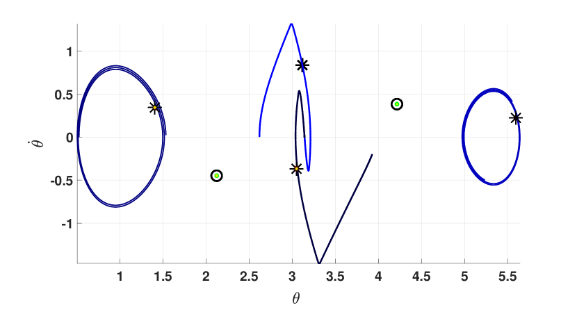
Figure 3: Data collection trajectories (solid lines) and query points ($\star$ and $\circ$) in state-space.

Moreover, the learned dynamics are more accurate for query points near the fixed point $\bar{x}_{\textnormal{eq}}=[\pi,0]^{\top}$ than for query points far away, as shown in Fig. 3. For example, at query points $\bar{x}=\{[1.40\ 0.34]^{\top},[3.05\ -0.37]^{\top},[3.11\ 0.84]^{\top},[5.60\ 0.22]^{\top}\}$, we see around $100\%$ decrease in the uncertainty range estimate as $N$ increases from $100$ to $4000$. The corresponding percentages for $\bar{x}=\{[4.21\ 0.38]^{\top},[2.12\ -0.45]^{\top}\}$ are just around $73\%$ and $34\%$ respectively.

VI-C Computation of Positive Invariant Set

For pendulum dynamics (19) in discrete-time, we use the BMI (5) of Proposition 5 to compute an ellipsoidal positive invariant set. In this specific example, we have used all the $N=4000$ samples from each of the previously collected four trajectories in Section VI-B. The number of intersecting ellipsoids $n_{I}$ in (5) is set as $n_{I}=2$. Fig. 4 shows the invariant set $\mathcal{X}_{I}\subseteq\mathcal{X}$, where $\mathcal{X}=[0,2\pi]\times[-2.5,2.5]$. To further check numerically that the set $\mathcal{X}_{I}$ in Fig. 4 is indeed a positive invariant set, we run simulations from six initial conditions inside the set. As seen in Fig. 4, all six trajectories stay within $\mathcal{X}_{I}$.

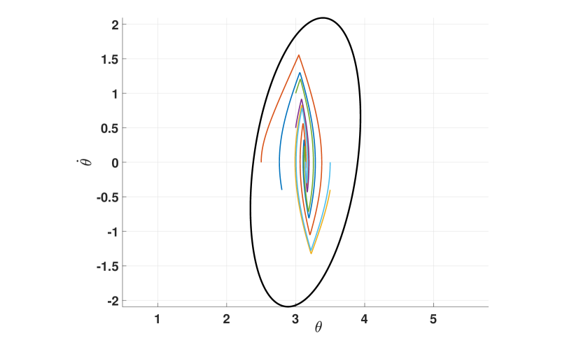
Figure 4: Invariant set (solid black line) computed using (5). Trajectories starting inside the set are contained within.

VII Conclusions

We presented a non-parametric technique for online modeling of systems with nonlinear Lipschitz dynamics. The key idea is to successively use measurements to approximate the graph of the function using envelopes described by quadratic constraints. Using techniques from convex optimization, we also computed a set valued estimate of the range of the unknown function at any given point in its domain, and a positive invariant set around a known equilibrium. We further highlighted the efficacy of the proposed methodology via a detailed numerical example.

-A Tractable Optimization Problems for Section V

-A1 SDP for Ellipsoidal Outer Approximation of $\mathcal{F}(x_{N})$

Following [35, Section 11.4] finding the the minimum trace ellipsoid $\textnormal{ell}(c(x_{N}),R(x_{N}))$ that satisfies (V-A) can be posed as an SDP using Schur complement rule as:

$$\begin{array}[]{llll}\displaystyle\min_{\xi}&\textnormal{trace}(R(x_{N}))\\ ~{}\text{s.t.}&\begin{bmatrix}p(x_{N})&q(x_{N})&-\mathbb{I}_{n}\\ q^{\top}(x_{N})&r(x_{N})&c^{\top}(x_{N})\\ -\mathbb{I}_{n}&c(x_{N})&-R(x_{N})\end{bmatrix}\preceq 0,\\ &\tau_{k}\geq 0,~{}\forall k=0,1,\dots,N-1,\\ &R(x_{N})\succ 0,\end{array}$$

where $\xi=\{R(x_{N}),c(x_{N}),\tau_{0},\dots,\tau_{N-1}\}$ and we have used the variable nomenclature

$$p(x_{N}) =-\sum\limits_{k=0}^{N-1}\tau_{k}\mathbb{I}_{n},~{}q(x_{N})=\sum\limits_{k=0}^{N-1}\tau_{k}f(x_{k}),$$

$$r(x_{N}) =-1-\sum\limits_{k=0}^{N-1}\tau_{k}\Big{(}-L^{2}(x_{N})^{\top}x_{N}+2L^{2}(x_{N})^{\top}x_{k}$$

$$~{}~{}~{}~{}~{}~{}~{}~{}~{}~{}~{}~{}~{}-L^{2}(x_{k})^{\top}(x_{k})+f^{\top}(x_{k})f(x_{k})\Big{)}.$$

-A2 Bisection Method for Positive Invariant Set Computation

Note that (5) is linear in $P_{j}$ for a fixed $\rho_{jm}$ and vice-versa. This facilitates using a bisection search on $\rho_{jm}$ until a feasible solution is obtained. For bounded $\mathcal{X}$, feasibility is guaranteed for some $\rho$ such that all $\rho_{jm}=\rho$ because of continuity of (5) as well as its feasibility for $\rho=0$. After iterating over $\rho_{jm}$, (5) is solved as a Linear Matrix Inequality (LMI)

$$\begin{array}[]{llll}\displaystyle\min_{P_{1},\dots,P_{n_{I}},\tau_{0},\dots,\tau_{N-1}}&\sum_{j=1}^{n_{I}}\textrm{trace}(P_{j})\\ \ \ ~{}~{}~{}~{}~{}~{}~{}~{}~{}\text{s.t.}&\eqref{eq:s_proc_invar},\\ &\tau_{k}\geq 0,~{}\forall k=0,1,\dots,N-1.\end{array}$$

-B Proofs

Proof of Lemma 1

For any $(x,f(x))\in G(f)$, we have from the Lipschitz inequality,

$$\|f(x)-f(y)\|\leq L\|x-y\|,\quad\forall y\in\mathcal{X},$$

and choosing $y=x_{k}$ for $k=0,1,\dots N-1$ in the above inequality, in view of Corollary 1 yields,

$$(x,f(x)) \in\mathcal{E}(x_{k}),\quad\forall k=0,1,\dots N-1,$$

$$\Rightarrow(x,f(x)) \in\bigcap_{k=0}^{N-1}\mathcal{E}(x_{k}).$$

Note the fact that $f$ is globally Lipschitz ensures that the intersections are non-empty. Since this was shown for any $(x,f(x))\in G(f)$, we can thus conclude that

$$G(f)=\bigcup_{x\in\mathcal{X}}(x,f(x))\subseteq\bigcap_{k=0}^{N-1}\mathcal{E}(x_{k}).$$

The other equalities follow from (8). $\blacksquare$

Proof of Proposition 3

We first prove the implication for when condition (1) holds. Let $k^{\star}$ be the time at which the system enters the $p$-periodic orbit, i.e., $\mathcal{O}_{p}(x_{k^{\star}})\subseteq\{x_{0},x_{1},x_{2},\dots\}$. From Lemma 1 we have $\mathbf{E}^{f}_{N}=\bigcap_{k=0}^{N-1}\mathcal{E}(x_{k})$ at any time $N$. For $N\geq k^{\star}+p$, consider the set

$$\mathbf{E}^{f}_{N+1} =\bigcap_{k=0}^{N}\mathcal{E}(x_{k})$$

$$=(\bigcap_{k=0}^{k^{\star}-1}\mathcal{E}(x_{k}))\cap(\bigcap_{k=k^{\star}}^{k^{\star}+p-1}\mathcal{E}(x_{k}))\cap(\bigcap_{k=k^{\star}+p}^{N}\mathcal{E}(x_{k})),$$

$$=\mathbf{E}^{f}_{k^{\star}+p}\cap(\bigcap_{k=k^{\star}+p}^{N}\mathcal{E}(x_{k})).$$

From Definition 5, we have that $x_{k}\in\mathcal{O}_{p}(x_{k^{\star}})$ for all $k=k^{\star}+p,\dots,N$. Using (9) and the fact that $f(\cdot)$ is globally Lipschitz on $\mathcal{X}$, we thus have $\mathbf{E}^{f}_{k^{\star}+p}\subseteq\mathcal{E}(x_{k})$, for all $k=k^{\star}+p,\dots,N$. Combining this implication with the definition of $\mathbf{E}^{f}_{N+1}$ above yields

$$\mathbf{E}^{f}_{N+1}=\mathbf{E}^{f}_{k^{\star}+p},\quad\forall N\geq k^{\star}+p,$$

and so $\mathbf{E}^{f}_{k^{\star}+p}$ is a fixed point for recursion (8).
Now we prove the implication for when condition (2) holds, i.e., $\lim_{k\rightarrow\infty}x_{k}=\bar{x}_{\textnormal{eq}}$. Since the sets $\mathbf{E}^{f}_{N}=\bigcap_{k=0}^{N-1}\mathcal{E}(x_{k})$ are non-increasing in the sense of (10), the following limit set is well defined

$$\mathbf{E}^{f}_{\star} =\lim_{N\rightarrow\infty}\mathbf{E}^{f}_{N}$$

$$=\lim_{N\rightarrow\infty}\bigcap_{k=0}^{N-1}\mathcal{E}(x_{k}),$$

$$=\lim_{N\rightarrow\infty}(\bigcap_{k=0}^{N-2}\mathcal{E}(x_{k}))\cap\mathcal{E}(x_{N-1}),$$

$$=\lim_{N\rightarrow\infty}\bigcap_{k=0}^{N-2}\mathcal{E}(x_{k})\cap\mathcal{E}(\lim_{N\rightarrow\infty}x_{N-1}).$$

The last equality follows from the property of product of convergent sequences because all the limits on both sides of the equation are well defined. Computing the limits then gives us the following equality

$$\mathbf{E}^{f}_{\star}=\mathbf{E}^{f}_{\star}\cap\mathcal{E}(\bar{x}_{\textnormal{eq}}).$$

Thus $\mathbf{E}^{f}_{\star}$ is a fixed point for recursion (8). $\blacksquare$

Proof of Theorem 1

From the definition $x_{0}$ in the theorem, we have that the sequence $\Big{\{}x_{k}\Big{\}}_{k=0}^{\infty}$ converges to the fixed point $\bar{x}_{\textnormal{eq}}$ of (1). From the definition of the convergence of a sequence, we have that for every $\epsilon>0$, there exists a $\bar{N}(\epsilon)$, such that

$$\|x_{k}-\bar{x}_{\textnormal{eq}}\|\leq\epsilon,\quad\forall k\geq\bar{N}(\epsilon).$$

The convergent sequence is a Cauchy sequence satisfying with the same $\epsilon$ and $\bar{N}(\epsilon)$ as above. That is,

$$\|x_{k_{1}}-x_{k_{2}}\|\leq 2\epsilon,\quad\forall k_{2},k_{1}\geq\bar{N}(\epsilon).$$ (21)

Consider a subsequent queried point $\bar{x}$ at most $\epsilon$ distance away from $\bar{x}_{\textnormal{eq}}$. We further have from the Lipschitz inequality,

$$\|f(x_{k_{1}})-f(\bar{x})\| \leq L\|x_{k_{1}}-\bar{x}\|.$$ (22)

From Proposition 4, we know that the possible values of $f(\bar{x})$ lie within a sphere of radius $L\|x_{k_{1}}-\bar{x}\|$ centered at $f(x_{k_{1}})$. The diameter of the above sphere bounds the maximum error in the estimate of $f(\bar{x})$, i.e.,

$$\|y-f(\bar{x})\|\leq 2L\|x_{k_{1}}-\bar{x}\|,\quad\forall y\in\mathcal{S}(x_{k_{1}},\bar{x}).$$

For $k_{1}$ chosen as in (21), the above inequality can be written as

$$\|y-f(\bar{x})\|\leq 4L\epsilon,\quad\forall y\in\mathcal{S}(x_{k_{1}},\bar{x}).$$

Now for another $k_{2}$ chosen as in (21) such that $f(x_{k_{1}})\neq f(x_{k_{2}})$, we have

$$\|f(x_{k_{2}})-f(\bar{x})\| \leq L\|x_{k_{2}}-\bar{x}\|.$$ (23)

The intersections of the envelopes constructed from (22) and (23) is depicted in Fig. 5.

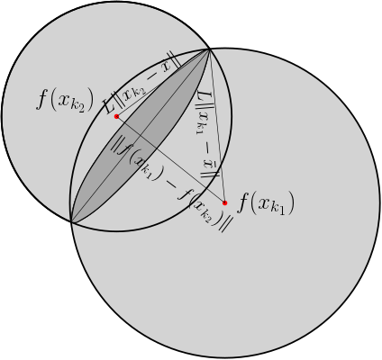
Figure 5: Intersection of set of possible values of $f(\bar{x})$, given two samples $x_{k_{1}}$, $x_{k_{2}}$

We thus obtain a tighter bound on the error in the estimate of $f(\bar{x})$ via the diameter of the $n-2$ dimensional sphere obtained at the intersection of $n-1$ dimensional spheres, as given by

$$\|y-f(\bar{x})\|\leq$$

$$2\sqrt{\frac{L^{2}(\|x_{k_{1}}-\bar{x}\|^{2}+\|x_{k_{2}}-\bar{x}\|^{2})-\|f(x_{k_{2}})-f(x_{k_{1}})\|^{2}}{2}},$$

$$\leq\textrm{min}(2L\|x_{k_{2}}-\bar{x}\|,2L\|x_{k_{1}}-\bar{x}\|)\leq 4L\epsilon,$$

$$\hfill\forall y\in\mathcal{S}(x_{k_{1}},\bar{x})\cap\mathcal{S}(x_{k_{2}},\bar{x})$$

$$\Rightarrow \max_{y\in\mathcal{S}(x_{k_{1}},\bar{x})\cap\mathcal{S}(x_{k_{2}},\bar{x})}\|y-f(\bar{x})\|\leq$$

$$2\sqrt{\frac{L^{2}(\|x_{k_{1}}-\bar{x}\|^{2}+\|x_{k_{2}}-\bar{x}\|^{2})-\|f(x_{k_{2}})-f(x_{k_{1}})\|^{2}}{2}},$$

$$\leq\textrm{min}(2L\|x_{k_{2}}-\bar{x}\|,2L\|x_{k_{1}}-\bar{x}\|)\leq 4L\epsilon$$

Taking intersections using all the envelopes collected (which are non-empty due to Lipschitz property of $f(\cdot)$ on $\mathcal{X}$) further shrinks the possible error and hence yields the desired result.

$\blacksquare$

Proof of Proposition 5

Consider any vector $[x^{\top}y^{\top}1]^{\top}\in\mathbb{R}^{2n+1}$ such that $x\in\mathcal{X}_{I}$ and $[x^{\top}y^{\top}]^{\top}\in G(f)$. Given that BMI (5) is feasible, we multiply $[x^{\top}y^{\top}1]^{\top}\in\mathbb{R}^{2n+1}$ on both sides of (5) for any $m\in\{1,2,\dots,n_{I}\}$ to get

$$\sum_{j=1}^{n_{I}}\begin{bmatrix}-\rho_{jm}P_{j}&0&\rho_{jm}P_{j}\bar{x}_{\textnormal{eq}}\\ 0&P_{m}&-P_{m}\bar{x}_{\textnormal{eq}}\\ \bar{x}^{\top}_{\textnormal{eq}}\rho_{jm}P_{j}&-\bar{x}^{\top}_{\textnormal{eq}}P_{m}&-\bar{x}^{\top}_{\textnormal{eq}}(\rho_{jm}P_{j}-P_{m})\bar{x}_{\textnormal{eq}}+\rho_{jm}-1\end{bmatrix}$$

$$~{}~{}~{}~{}~{}~{}~{}~{}~{}~{}~{}~{}~{}~{}~{}~{}~{}~{}~{}~{}~{}~{}~{}~{}~{}~{}~{}~{}~{}~{}~{}~{}~{}~{}~{}~{}~{}~{}~{}~{}~{}~{}~{}~{}~{}~{}~{}~{}~{}~{}~{}-\sum\limits_{k=0}^{N-1}\tau_{k}Q_{L}^{f}(x_{k})\preceq 0,$$

$$\Rightarrow\sum_{j=1}^{n_{I}}-\rho_{jm}\begin{bmatrix}x\\ 1\end{bmatrix}^{\top}\bar{P}_{j}\begin{bmatrix}x\\ 1\end{bmatrix}+n_{I}\begin{bmatrix}y\\ 1\end{bmatrix}^{\top}\bar{P}_{m}\begin{bmatrix}y\\ 1\end{bmatrix}$$

$$~{}~{}~{}~{}~{}~{}~{}~{}~{}~{}~{}~{}~{}~{}~{}~{}~{}~{}~{}~{}~{}~{}~{}~{}~{}~{}~{}~{}~{}~{}~{}~{}~{}~{}~{}~{}-\begin{bmatrix}x\\ y\\ 1\end{bmatrix}^{\top}\sum\limits_{k=0}^{N-1}\tau_{k}Q_{L}^{f}(x_{k}))\begin{bmatrix}x\\ y\\ 1\end{bmatrix}\leq 0,$$

$$\Rightarrow\begin{bmatrix}y\\ 1\end{bmatrix}^{\top}\bar{P}_{m}\begin{bmatrix}y\\ 1\end{bmatrix}\leq 0,\ \forall m=1,2\dots,n_{I},$$

where $\bar{P}_{j}=\begin{bmatrix}P_{j}&-P_{j}\bar{x}_{\textnormal{eq}}\\ -\bar{x}^{\top}_{\textnormal{eq}}P_{j}&\bar{x}^{\top}_{\textnormal{eq}}P_{j}\bar{x}_{\textnormal{eq}}-1\end{bmatrix}$. The last implication follows from the fact $x\in\mathcal{X}_{I}$ and $G(f)\subseteq\mathbf{E}^{f}$ (as proved in Lemma 1). The last inequality further implies that $G(f)\ni y\in\mathcal{X}_{I}$, for all $x\in\mathcal{X}_{I}$, and hence, that $\mathcal{X}_{I}$ is invariant. $\blacksquare$

References

• [1] B. Recht, “A tour of reinforcement learning: The view from continuous control,” Annual Review of Control, Robotics, and Autonomous Systems, vol. 2, pp. 253–279, 2019.
• [2] U. Rosolia, X. Zhang, and F. Borrelli, “Data-driven predictive control for autonomous systems,” Annual Review of Control, Robotics, and Autonomous Systems, vol. 1, pp. 259–286, 2018.
• [3] D. P. Bertsekas and D. A. Castanon, “Adaptive aggregation methods for infinite horizon dynamic programming,” IEEE Transactions on Automatic Control, vol. 34, no. 6, pp. 589–598, 1989.
• [4] C. J. Watkins and P. Dayan, “Q-learning,” Machine learning, vol. 8, no. 3-4, pp. 279–292, 1992.
• [5] M. Krstic, I. Kanellakopoulos, and P. V. Kokotovic, Nonlinear and adaptive control design.   Wiley, 1995.
• [6] S. Sastry and M. Bodson, Adaptive control: Stability, convergence and robustness.   Courier Corporation, 2011.
• [7] J. Friedman, T. Hastie, and R. Tibshirani, The elements of statistical learning.   Springer series in statistics New York, 2001, vol. 1, no. 10.
• [8] T. J. Hastie, “Generalized additive models,” in Statistical models in S.   Routledge, 2017, pp. 249–307.
• [9] T. Hothorn, F. Bretz, and P. Westfall, “Simultaneous inference in general parametric models,” Biometrical journal, vol. 50, no. 3, pp. 346–363, 2008.
• [10] W. K. Härdle, M. Müller, S. Sperlich, and A. Werwatz, Nonparametric and semiparametric models.   Springer Science & Business Media, 2012.
• [11] M. Green and J. B. Moore, “Persistence of excitation in linear systems,” Systems & control letters, vol. 7, no. 5, pp. 351–360, 1986.
• [12] Z. Ghahramani and S. T. Roweis, “Learning nonlinear dynamical systems using an em algorithm,” in Advances in neural information processing systems, 1999, pp. 431–437.
• [13] N. Kalouptsidis, G. Mileounis, B. Babadi, and V. Tarokh, “Adaptive algorithms for sparse system identification,” Signal Processing, vol. 91, no. 8, pp. 1910–1919, 2011.
• [14] C. E. Rasmussen, “Gaussian processes in machine learning,” in Summer School on Machine Learning.   Springer, 2003, pp. 63–71.
• [15] J. Fan et al., “Local linear regression smoothers and their minimax efficiencies,” The annals of Statistics, vol. 21, no. 1, pp. 196–216, 1993.
• [16] U. Rosolia and F. Borrelli, “Learning how to autonomously race a car: a predictive control approach,” arXiv preprint arXiv:1901.08184, 2019.
• [17] E. Schuster, S. Yakowitz et al., “Contributions to the theory of nonparametric regression, with application to system identification,” The Annals of Statistics, vol. 7, no. 1, pp. 139–149, 1979.
• [18] T. Armstrong and M. Kolesár, “Simple and honest confidence intervals in nonparametric regression,” Cowles Foundation Discussion Paper, 2018.
• [19] F. Berkenkamp, M. Turchetta, A. Schoellig, and A. Krause, “Safe model-based reinforcement learning with stability guarantees,” in Advances in Neural Information Processing Systems, 2017, pp. 908–918.
• [20] T. Koller, F. Berkenkamp, M. Turchetta, and A. Krause, “Learning-based model predictive control for safe exploration,” in 2018 IEEE Conference on Decision and Control (CDC).   IEEE, 2018, pp. 6059–6066.
• [21] F. Blanchini, “Set invariance in control,” Automatica, vol. 35, no. 11, pp. 1747–1767, 1999.
• [22] I. Kolmanovsky and E. G. Gilbert, “Theory and computation of disturbance invariant sets for discrete-time linear systems,” Mathematical Problems in Engineering, vol. 4, no. 4, pp. 317–367, 1998.
• [23] I. Pólik and T. Terlaky, “A survey of the s-lemma,” SIAM review, vol. 49, no. 3, pp. 371–418, 2007.
• [24] W. Rudin et al., Principles of mathematical analysis.   McGraw-hill New York, 1964, vol. 3.
• [25] A. Chakrabarty, D. K. Jha, and Y. Wang, “Data-driven control policies for partially known systems via kernelized lipschitz learning,” in 2019 American Control Conference (ACC).   IEEE, 2019, pp. 4192–4197.
• [26] M. Tanaskovic, L. Fagiano, R. Smith, and M. Morari, “Adaptive receding horizon control for constrained MIMO systems,” Automatica, vol. 50, no. 12, pp. 3019–3029, 2014.
• [27] M. Bujarbaruah, X. Zhang, and F. Borrelli, “Adaptive MPC with chance constraints for FIR systems,” in 2018 Annual American Control Conference (ACC), June 2018, pp. 2312–2317.
• [28] M. Bujarbaruah, X. Zhang, M. Tanaskovic, and F. Borrelli, “Adaptive MPC under time varying uncertainty: Robust and Stochastic,” arXiv preprint arXiv:1909.13473, 2019.
• [29] D. Bertsekas and I. Rhodes, “Recursive state estimation for a set-membership description of uncertainty,” IEEE Transactions on Automatic Control, vol. 16, no. 2, pp. 117–128, 1971.
• [30] M. Fazlyab, M. Morari, and G. J. Pappas, “Safety verification and robustness analysis of neural networks via quadratic constraints and semidefinite programming,” arXiv preprint arXiv:1903.01287, 2019.
• [31] A. Megretski and A. Rantzer, “System analysis via integral quadratic constraints,” IEEE Transactions on Automatic Control, vol. 42, no. 6, pp. 819–830, 1997.
• [32] Z. Zhou, “Periodic orbits on discrete dynamical systems,” Computers & Mathematics with Applications, vol. 45, no. 6-9, pp. 1155–1161, 2003.
• [33] J. M. Ortega, “Stability of difference equations and convergence of iterative processes,” SIAM Journal on Numerical Analysis, vol. 10, no. 2, pp. 268–282, 1973.
• [34] A. Ben-Tal, L. El Ghaoui, and A. Nemirovski, Robust optimization.   Princeton University Press, 2009, vol. 28.
• [35] G. C. Calafiore and L. El Ghaoui, Optimization models.   Cambridge university press, 2014.
• [36] S. Boyd and L. Vandenberghe, Convex optimization.   New York, NY, USA: Cambridge University Press, 2004.
• [37] Z. Jarvis-Wloszek, R. Feeley, Weehong Tan, Kunpeng Sun, and A. Packard, “Some controls applications of sum of squares programming,” in 42nd IEEE International Conference on Decision and Control, vol. 5, Dec 2003, pp. 4676–4681.
• [38] S. H. Nair and R. N. Banavar, “Discrete optimal control of interconnected mechanical systems,” 11th IFAC Symposium on Nonlinear Control Systems (NOLCOS), 2019.