Hilbert Space Fragmentation and Ashkin-Teller Criticality
in Fluctuation Coupled Ising Models

Abstract

We discuss the effects of exponential fragmentation of the Hilbert space on phase transitions in the context of coupled ferromagnetic Ising models in arbitrary dimension with special emphasis on the one dimensional case. We show that the dynamics generated by quantum fluctuations is bounded within spatial partitions of the system and weak mixing of these partitions caused by global transverse fields leads to a zero temperature phase with ordering in the local product of both Ising copies but no long range order in either species. This leads to a natural connection with the Ashkin-Teller universality class for general lattices. We confirm this for the periodic chain using quantum Monte Carlo simulations. We also point out that our treatment provides an explanation for pseudo-first order behavior seen in the Binder cumulants of the classical frustrated $J_{1}-J_{2}$ Ising model and the $q=4$ Potts model in 2D.

I Introduction

The nature of quantum phase transitions has generated a large amount of interest in the context of magnetic systems. Some of the important fields in which the physics at a quantum phase transition plays an essential role are order to order transitions with exotic emergent symmetries Senthil ; Nahum ; NahumX ; Bowen , determining the ability of quantum annealing to solve computational problems qa1 ; qa2 ; qa3 , and the understanding of field theoretic frameworks to describe low energy physics of discrete models IsingCFT ; PottsFT ; ClockFT . Crucial to these topics is the structure of low energy excitations at critical points, especially those which have spatial restrictions such as fractons FracRev ; FracCham . Recently these restricted dynamics have been seen as a consequence of spatial “fragmentation” of the Hilbert space ETH1 ; ETH2 . Fragmentation describes the consequence of block diagonalization of a Hilbert space into an exponentially large number of sectors, with spatial structure corresponding to the states making up a sector. A similar phenomenon has been observed in quantum dimer models as well Sha , although a spatial pattern corresponding to sectors has not been identified in this case.

In this article, we address another more general manifestation of the phenomenon of Hilbert space fragmentation by introducing a simple model whose Hilbert space breaks into an exponentially large number of sectors, each of which has interesting spatial patterns which limit the growth of the correlation length. We draw connections between the nature of this fragmentation and the partitions of natural numbers, and discuss in the context of this model the effects of the underlying lattice it is set on in terms of its percolation properties and the structure of excitations they lead to. We study the nature of eigenstates and energies for the 1D case and briefly discuss our expectations from this model when it is placed in contact with a thermal bath. We then turn to the effects of adding symmetry breaking quantum perturbations at zero temperature, where we find behavior suggestive of a phase with partial ordering. We draw a comparison with the Ashkin-Teller model ATintro , where a similar phase is seen, and argue for a complete mapping between our model and the Ashkin-Teller model. We quantitatively check this mapping for the 1D case using quantum Monte Carlo simulation, and find consistency with the range of continuously varying exponents already known to exist for the Ashkin-Teller universality class Cardy ; ATsource . We also point out that the partially ordered phase provides an explanation for pseudo-first order behavior observed in the Binder cumulants at some continuous phase transitions, e.g. 2D $q=4$ Potts and $J_{1}-J_{2}$ frustrated Ising models JinSan .

The outline of the paper is as follows: In Sec. II, we present the model, describe the fragmented Hilbert space structure, and point out the few general constraints required to get this feature. We also present a detailed study of the energy spectrum for a periodic chain. In Sec. III, we incorporate the perturbation which takes the systems away from the fragmented Hilbert space structure and briefly discuss the expected effect on dynamics. This is followed by a description of the Ashkin-Teller universality class along with a general mapping to our system, which we check in detail for the 1D system through numerical results. In Sec. IV, we describe pseudo-first order behavior and the role of the partially ordered phase in generating a behavior similar to the 4-state Potts and other related models. In Sec. V, we conclude with a brief summary and discussion.

II Fluctuation Coupled Ising Models and Fragmentation

We will introduce the fragmentation of the Hilbert space and its consequences in the context of a coupled Ising model made out of two Ising species, $\sigma$ and $\tau$, with the following Hamiltonian:

$$H=-\frac{s}{2}\sum_{\langle i,j\rangle}\big{(}\sigma^{z}_{i}\sigma^{z}_{j}+\tau^{z}_{i}\tau^{z}_{j}\big{)}-(1-s)\sum_{i}\sigma^{x}_{i}\tau^{x}_{i}.$$ (1)

Here, $\langle i,j\rangle$ refers to nearest neighbors and $s$ is the tuning parameter used to drive the ground state from a paramagnet ($s=0$) to a ferromagnet ($s=1$). This model can also be written using just a single species ($\sigma$) which lives on a larger lattice and comprises of two copies of the original lattice connected in a bilayer fashion.

The Hamiltonian described in Eq. (1) possesses a local conserved quantity, $\sigma^{z}_{i}\tau^{z}_{i}$, associated with each site of the lattice. This is due to the particular form of the quantum fluctuation, $\sigma^{x}_{i}\tau^{x}_{i}$, which commutes with $\sigma^{z}_{i}\tau^{z}_{i}$. As $\sigma^{z}_{i}\tau^{z}_{i}$ is a conserved quantity, it takes well defined values, which are $+1$ and $-1$ in this case. For a lattice with $N$ sites, the set $\{\sigma^{z}_{i}\tau^{z}_{i}\}^{N}_{i=0}$ can take $2^{N}$ values, implying that the Hamiltonian can be broken into $2^{N}$ blocks. An example of one such block is shown in Fig. 1 for a square lattice, where $+/-$ denote the value of $\sigma^{z}_{i}\tau^{z}_{i}$ at each site. In terms of the individual $\sigma$ and $\tau$ spins, we shall use $0$ to denote the state $\sigma^{z}(\tau^{z})=-1$ and $1$ to denote $\sigma^{z}(\tau^{z})=+1$. Now the four possible states in the $z$-basis on a single site are $\{00,01,10,11\}$ where the first number denotes the state of the $\sigma$ spin (0 or 1) and the second denotes the $\tau$ spin. The constraint of a particular value for $\sigma^{z}_{i}\tau^{z}_{i}$ reduces the number of basis states at site $i$ to two. This implies each block is a $2^{N}\times 2^{N}$ matrix.

For the rest of our analysis, we will assume that we have block diagonalized the Hamiltonian in Eq. (1), and that any quantum state of the system belongs only to one of these blocks. In addition to the block structure due to the conserved quantities described above, there is a further fragmentation within each block. This is developed below for the cases of an arbitrary lattice and a periodic chain.

II.1 Arbitrary Lattice

We begin by considering a system which lives on an arbitrary lattice or dimensionality and examine the spin degrees of freedom. We show below that for nearest neighboring sites $i$ and $j$, if the state of the system belongs to a block such that $\sigma^{z}_{i}\tau^{z}_{i}\neq\sigma^{z}_{j}\tau^{z}_{j}$, then this pair of sites can be considered to be non-interacting.

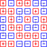
Figure 1: A fragment arrangement for the square lattice with interacting sites connected by dotted lines. The +’s and -’s denote the value of $\sigma^{z}_{i}\tau^{z}_{i}$ at each site.

First consider $\sigma^{z}_{i}\tau^{z}_{i}=\sigma^{z}_{j}\tau^{z}_{j}=+1$, with the state $00$ on site $i$ and the state $11$ on site $j$. The energy cost of such an arrangement due to the classical term $-(\sigma^{z}_{i}\sigma^{z}_{j}+\tau^{z}_{i}\tau^{z}_{j})$ is -2 (in units of the ferromagnetic coupling). This can be maximized by switching $11\to 00$ on site $j$, which is allowed by $\sigma^{z}_{j}\tau^{z}_{j}=+1$. If the constraint on site $j$ is instead chosen to be $\sigma^{z}_{j}\tau^{z}_{j}=-1$, then site $j$ hosts either $01$ or $10$, and the energy associated with the arrangement of states on $i$ and $j$ will always be 0, as one of the bonds (either $\sigma\sigma$ or $\tau\tau$) is always broken while the other is always satisfied. This implies that, from energy considerations, states $01$ and $10$ are equivalent if site $i$ hosts $00$. It follows that, if $\sigma^{z}_{i}\tau^{z}_{i}=\sigma^{z}_{j}\tau^{z}_{j}$, then they have an Ising bond of strength $s$ between them, else, they are non-interacting. If we now consider a typical set of values of $\{\sigma^{z}_{i}\tau^{z}_{i}\}^{N}_{i=0}$ (corresponding to a block) as shown in Fig. 1 for a 2D lattice, we see that the system has essentially broken into several smaller Ising models which co-exist on the lattice. We call each of these smaller Ising models a fragment. For simple regular lattices, such as a 1D chain, square or cubic lattice with periodic conditions, the fragment arrangements can be related to the partitions of natural numbers Part1 ; Part2 . This connection will be later illustrated using a periodic chain. It is worth noting here that this argument applies also for a more general classical term of the form $f(\sigma^{z}_{0},\tau^{z}_{0},...,\sigma^{z}_{N},\tau^{z}_{N})$, which is symmetric under the exchange of the Ising species, $\sigma\to\tau$. As this function must be symmetric for all spin configurations, the constraint would need to be satisfied for each bond, and the above argument would be valid. There may be other convoluted ways to satisfy the symmetry requirement for certain complicated functions.

The phenomenon described above is similar to the fragmentation discussed in recent work in the context of the eigenstate thermalization hypothesis (ETH) ETH1 ; ETH2 and has also been studied in disordered Floquet circuits composed of Clifford gates ACCL . This phenomenon has also been observed numerically in quantum dimer models with restricted dynamics, but a similar real space geometric way to understand the same has not been identified in that context Sha .

One of the key features of the fragmentation of real space into components is that the correlation length in a particular block is bounded by the spatial extent of the largest clusters in the corresponding fragment arrangement. This feature depends crucially on the restricted dynamics generated by $\sigma^{x}_{i}\tau^{x}_{i}$ and the classical term allowing a degeneracy in energies. If the classical term were to be augmented by adding an interaction of the form $-\sigma^{z}_{i}\tau^{z}_{j}$ which breaks the $\sigma\to\tau$ symmetry, the non-interacting nature would be lost as the state $00$ on site $i$ would now prefer $10$ on site $j$ over $01$. Due to this term, each spin species has a global pattern specific to which block the state belongs to, and fluctuations would occur around this pattern in the large $s$ limit. The maximal correlation length in every block grows to the system size in the presence of such a term, although the details of this growth depend on the structure of the particular block. These arguments illustrate that, although the quantum term determines the block structure, interacting units within a block may be controlled by the choice of classical terms. Careful choice of tuning parameters can also create a scenario where there are two length scales, one associated with the growth of correlation within a component and the other with the growth across components. If we were to require that the symmetry in $\sigma\to\tau$ be maintained, an additional term would have to be added to ensure that the state $00$ does not favor one of $01$ or $10$, and the physics would again be the same as the Hamiltonian in Eq. (1).

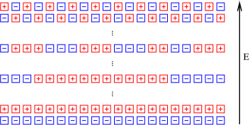
Figure 2: Fragment arrangements sorted by energy with reference blocks making up the lowest energy region and energy increasing bottom to top.

As a particular block in the Hamiltonian can be thought of as a configuration where each site is assigned either $+1$ or $-1$ with probability $1/2$, it can also be written in terms of a percolation problem where a particular site is occupied or left empty. If the percolation threshold for the particular lattice is below $1/2$, most blocks will have a giant fragment and this may have consequences on the correlation length as far above the percolation threshold, almost all blocks will have diverging length scales, leading to a continuous transition. The universality class for the transition may relate to those of diluted Ising models above the percolation threshold, which have been studied in the context of thermal and quantum phase transitions Perc1 ; Perc2 ; Perc3 . We are unable to study this aspect of the problem in the context of the periodic chain as the percolation threshold in 1D is unity, which means none of the fragment arrangements percolate except the two blocks which correspond to all sites having the same value for $\sigma^{z}_{i}\tau^{z}_{i}$. It is also noteworthy that, due to this fragmentation, the dynamics generated by $\sigma^{x}_{i}\tau^{x}_{i}$ reduces to the dynamics within the fragments and no inter-fragment correlations are introduced. In 2D and higher, the fragments would in general represent non-integrable systems which thermalize within their boundaries but not with the entire system. This implies that the system would not reach a thermal distribution and would not exhibit characteristics such as volume law entanglement entropy which would be expected of thermalizing systems.

II.2 Periodic Chain

Now we specialize to the case of a periodic chain with $L$ sites and consider the eigenstates and eigenenergies for various $s$. In the ferromagnetic limit ($s=1$), the lowest energy belongs to two blocks, one with $\sigma^{z}_{i}\tau^{z}_{i}=+1$ for all $i$, and the other $\sigma^{z}_{i}\tau^{z}_{i}=-1$ for all $i$. We shall refer to these two blocks as the reference blocks for this model, as they are the easiest to analyze and map exactly to the simple transverse field Ising chain. These blocks have $L$ activated bonds, whereas all other blocks have at least one pair of nearest neighbor sites which are non-interacting, leading to loss of the energy which could potentially be gained from that Ising bond. The first excited level in the ferromagnetic limit is made out of all blocks which have two fragments each, one with all $\sigma^{z}_{i}\tau^{z}_{i}=+1$ and the other with all $\sigma^{z}_{i}\tau^{z}_{i}=-1$, as these arrangements have $L-2$ activated bonds. In the limit of $s=0$, all the Ising bonds are switched off and all $2^{L}$ blocks are degenerate. The fragment arrangement of any block can be seen as a sum of independent Ising chains of various lengths. As the energy density of a longer Ising chain is always larger in magnitude than a shorter chain for all $s$ other than $s=0$ and $s=1$, the reference blocks, which comprise a single periodic chain of length $L$, always form the lowest energy manifold. A schematic energy spectrum classification for general $s$ can be seen in Fig 2.

As each block can be made up of many smaller chains, the energy spectrum of this Hamiltonian hosts a large amount of degeneracy. This can be understood by recognizing that many blocks share the same number and sizes of chains, and each block carries a different ordering of the chains. As the energy of a block is simply the sum of the energies of individual chains, the arrangement of chains that makes up a particular block does not play any role in calculating the energy; only the number and sizes of chains control the energy. Following this line of thought, we can now map our energy spectrum to the partitions of the natural number $L$, where each partition is defined as a set of smaller pieces whose lengths sum to $L$. For example the partitions for $L=4$ are:

$$\begin{split}4=3+1=2+2=2+1+1=1+1+1+1\end{split}$$ (2)

It was shown Partm that the number of partitions $p(L)$ of a natural number $L$ asymptotically behaves as $\log p(L)\approx C\sqrt{L}$ with $C=\pi\sqrt{2/3}$. Due to periodic boundary conditions, the only allowed partitions for the chain arrangements are those which have an even number of chains. It follows that the number of energy levels in addition to the reference level are the number of even partitions of the number $L$. We observe that this number quickly approaches half the asymptotic value for $L\geq 10$. If we now consider a particular block and study the growth of its correlation length as we change $s$ from the paramagnetic regime to the ferromagnetic regime, we would find that the correlation length grows until it reaches an upper bound which must be smaller than the largest chain in the partition corresponding to that block. If the largest chain is much smaller than system size the ground state of this block can never develop long range order. The statistics of different blocks along with their energies now control how much they contribute to the ground state of the total system in the presence of a temperature or symmetry breaking quantum fluctuation which allows them to mix.

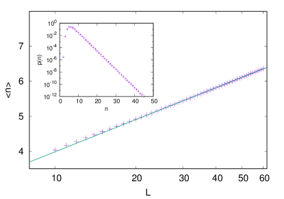
Figure 3: Average size of the largest fragment in a block plotted as a function of the system size $L$ for a periodic chain and fit to the form $\braket{n}\approx a+b\log(L)$ with $b=1.32(1)$. Inset: The probability distribution of the size of the largest fragment, which shows an exponential tail.

An added level of complexity is brought in by observing that each partition of the number $L$ corresponds to a different number of chain arrangements, i.e, blocks. The combinatorial factor related to this can be calculated using the following arguments. A particular arrangement of the chains in a partition can correspond to only two arrangements for the signs of $\sigma^{z}_{i}\tau^{z}_{i}$, as the moment a value is chosen for a chain, all others must be chosen in accordance with it to ensure the condition that the pieces are non-interacting. Taking this into account along with all the permutations of a particular partition and the translation invariance of the system, we conclude that the number of blocks $b(p)$ that correspond to that particular partition $p$ of the system size $L$ with an even number of chains $N$, is

$$b(p)=2L\frac{(N-1)!}{k_{1}!k_{2}!...k_{L}!},$$ (3)

where there $k_{i}$ is the number of pieces of length $i$, and we use $0!=1$. For example, the partition of system size $L=20$ given by $4+3+3+2+2+2+1+1+1+1$ has $N=10$ with $k_{1}=4$, $k_{2}=3$, $k_{3}=2$, $k_{4}=1$, and $k_{i}=0$ for all other $i=5,...,20$. We have checked Eq. (3) against exact enumeration. Although the average size of the largest chain in a partition where all partitions are sampled with equal weight goes as $O(\sqrt{L}\log(L))$ Partm , we find numerically (Fig. 3) that the added suppression caused by the factor in Eq. (3) reduces this to $O(\log(L))$.

We find numerically that the average size, $\braket{n}$, of the largest chain in the fragment arrangement corresponding to a random block follows the relation $\braket{n}=a+b\log(L)$, as seen in Fig 3 for $L=20,..,60$. We also study the probability distribution of the size of the largest chain in a random block chosen with uniform probability and find exponential tails for $p(n)$ for $n>\braket{n}$ (shown in inset of Fig 3 for a 60 site chain). This suggests that, if the system is allowed to choose a block at random, the largest chain in the chosen block will be much smaller than system size with a probability $\to 1$, thus leading to a severe limitation on the growth of correlation length.

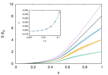
Figure 4: Energy levels for the Hamiltonian defined in Eq. (1) for system size $L=10$, as a function of tuning parameter $s$, seen to converge in $s=0$ limit and approach the spectrum of the classical Ising chain in $s=1$ limit. Inset: The minimum gap at $s=0.5$ as a function of $1/L$; extrapolating to $1/L=0$ gives a minimum gap of 0.31835(2).

The probability distribution with which the system samples different blocks depends on the terms connecting different blocks and the relative ground state energies of different blocks. As discussed above, the ground state of the entire system is always made out of the two blocks which have the same value of $\sigma^{z}_{i}\tau^{z}_{i}$ on all sites. The opposite limit is again made up of just two blocks, which are the blocks where all odd sites have the same value of $\sigma^{z}_{i}\tau^{z}_{i}$, and the even sites have the opposite value (Fig 2). Each of these breaks into $L$ disconnected spins, as no nearest neighbor spins have a ferromagnetic bond between them. This implies that every spin is polarized in the $\pm x$-direction due to the $\sigma^{x}\tau^{x}$ term with an energy of $-s$, making the total energy of the state $-Ls$. We can assume that the ground state energy for the reference blocks can be written as $-L\epsilon(L,s)$ where $\epsilon(L,s)$ is the energy density for a periodic chain of length $L$ at tuning parameter value $s$. These two extremes set the range of energies which can be occupied by all other blocks. Another general trend to be expected from the lowering of the energy due to larger system size would be to have partitions with the largest chains having ground states which occupy lower energy levels (Fig. 2). As we have seen from the distribution of partitions, these levels would contain a relatively small number of ground states as the parent blocks must contain long chains. Also, all the energies must converge in the $s=0$ limit, as the ferromagnetic term switches off, leaving all blocks equivalent in energy.

The above arguments give us a fair idea of the energy level diagram for the ground states in all the blocks. We present a detailed study of the $L=10$ case in Fig. 4, obtained using Lanczos diagonalization, which captures the essential features. An important region of the energy level diagram is $s\approx 0.5$, as the simple Ising chain undergoes a continuous quantum phase transition at this point. In an Ising chain, the correlation length grows continuously with increasing $s$ for $s<0.5$ and at the transition the correlation length reaches the system size. If the gap to a large number of blocks vanishes at this point, the correlation length would acquire large contributions from the other blocks in the presence of arbitrarily small coupling across blocks, which would lead to a capping on the correlation length. As the gap must once again open in the ferromagnetic regime, the system will drop back into the fully polarized state with large correlation length. This mechanism can create a jump in the correlation length, which is a hallmark of a first order phase transition. This is a heuristic argument which does not take into account the nature of the coupling to other blocks. Using the Jordan Wigner transformation to map the Ising chains to non-interacting fermions YoungReiger , we find that the gap at $s=0.5$ indeed converges to a non-zero value with increasing size. This is shown in the inset of Fig 4 for system sizes up to $L=512$, along with a finite size extrapolation, leading to a gap of 0.31835(2) in the thermodynamic limit. This is expected for higher dimensions as well, as the lowest block above the ground state block must necessarily have at least one missing ferromagnetic bond which contributes a finite amount to the energy. Our analysis also showed that the first state above the ground state of the reference blocks belongs to a block which breaks into a fragment which has a single site and a fragment which has $L-1$ sites. At $s=0.5$, blocks with this type of structure have the minimum energy amongst all blocks with only two fragments.

II.3 Fluctuations between blocks and block mixing

Here we discuss the effects of block mixing for arbitrary lattices with $N$ sites. One of the easier ways to allow the system to access all possible blocks would be to couple it to a thermal bath which provides an inverse temperature $\beta$. Assuming that the ground state energies of all the blocks is $O(N)$ (an example of which we see in the energy level diagram in Fig. 4), the contribution of the blocks with relatively small fragments or “restricted” blocks ($Z_{r}$) in the partition function is $Z_{r}=e^{-\beta E}D_{r}$, where $D_{r}$ is the degeneracy of the blocks. As we have seen that this degeneracy$\to 2^{N}$ and $E\propto N$, a finite $\beta$ will not necessarily suppress these levels, and there can exist a range of temperatures where these levels can mediate a transition with limited correlation length, i.e, a first order transition. Finite temperature would allow thermal fluctuations which can jump across blocks and in this way wash out the block structure as well. This cannot be studied in our analysis of the 1D chain as it is known that any non-zero temperature leads to disorder in the Ising chain and the phase transition is thus completely washed out. For higher dimensional systems this mechanism can lead to interesting crossover physics between the continuous quantum phase transition and the thermal phase transition of the classical system expected at any finite temperature. A coupling across blocks can also be achieved by a weak global transverse field or other more complicated quantum fluctuations. Non-perturbative numerical results, which layout the entire phase diagram in the presence of a transverse field, are presented in the following section.

III Perturbations and Ashkin-Teller Criticality

We now connect the different blocks using a weak perturbation which breaks the conservation of $\sigma^{z}_{i}\tau^{z}_{i}$. In spin language this corresponds to a global transverse field, leading to a Hamiltonian of the form

$$\begin{split}H=&\frac{-s}{2}\sum_{\langle i,j\rangle}\big{(}\sigma^{z}_{i}\sigma^{z}_{j}+\tau^{z}_{i}\tau^{z}_{j}\big{)}\\ &-(1-s)\sum_{i}\big{[}p\sigma^{x}_{i}\tau^{x}_{i}+(1-p)(\sigma^{x}_{i}+\tau^{x}_{i})\big{]}.\end{split}$$ (4)

Here, the $\sigma^{x}(\tau^{x})$ operator switches $00\to 10\ (00\to 01)$, effectively mixing blocks. In the weak perturbative limit of $(1-p)\ll 1$, this can be seen as connecting blocks which have differing values for $\sigma^{z}_{i}\tau^{z}_{i}$ for only a few sites, i.e those which have similarly sized chains in a similar arrangement. For smaller $p$, blocks which have chains of substantially different sizes would begin to couple as well, which would imply that the bound on the correlation length would weaken as the system can now build in longer correlations through a combination of blocks for the same value of $s$. In the opposite limit of $p\to 0$, blocks are strongly coupled, and the system can also be seen as two copies of transverse field Ising models. This suggests that the system would undergo a continuous transition, which would be in the Ising universality class of the appropriate dimension.

For $p=1$, the ground state sector is exactly a transverse field Ising model on the appropriate lattice, as discussed in the previous section. In this limit, for all $s\in[0,1]$, $M_{P}=\frac{1}{N}\sum_{i}\sigma^{z}_{i}\tau^{z}_{i}=\pm 1$ as all $\sigma^{z}_{i}\tau^{z}_{i}$ are either +1 or -1 for the reference blocks. Here $P$ signifies polarization order, a term which is used in literature discussing the Ashkin-Teller (AT) model ATintro ; ATsource , which is the higher dimensional classical equivalent of our model. This will be discussed in more detail later in this section. For $s\to 1$, $\sigma^{z}$ and $\tau^{z}$ are each disordered and with reducing $s$, they undergo an Ising transition where they develop long range order. For $p<1$, at $s=0$ the paramagnet phase has no long range order in fragment arrangements or either of the spin species as the perturbation allows complete access to Hilbert space. The conditions describe three phases, 1) complete paramagnetic phase with $\langle M^{2}_{P}\rangle=\langle M^{2}_{\sigma}\rangle=\langle M^{2}_{\tau}\rangle=0$, 2) polarization ordering with $\langle M^{2}_{P}\rangle\neq 0,\langle M^{2}_{\sigma}\rangle=\langle M^{2}_{\tau}\rangle=0$, and 3) ferromagnet with $\langle M^{2}_{P}\rangle\neq 0,\langle M^{2}_{\sigma}\rangle=\langle M^{2}_{\tau}\rangle\neq 0$.

These three phases can also be understood in terms of the well-studied AT modelATsource . Our model of fluctuation-coupled Ising systems can be mapped onto this classical model using the $d$-dimensional quantum to $d+1$-dimensional classical mapping based on the path integral formalism. For a quantum system, the partition function, given by Tr$[e^{-\beta H}]$, can be expanded in imaginary time using $\beta=n\Delta\tau$. This leads to a partition function of a classical model in a higher dimension qtoc , where $\sigma^{x}_{i}$ in the quantum model is replaced by a bond $\sigma^{z}_{i}\sigma^{z}_{i+1}$, in the imaginary time direction. This substitution to Eq. (4) leads to an anisotropic version of the AT model in $d+1$ dimensions. The isotropic AT Hamiltonian is as follows:

$$H=-J\sum_{\langle i,j\rangle}\sigma^{z}_{i}\sigma^{z}_{j}-J\sum_{\langle i,j\rangle}\tau^{z}_{i}\tau^{z}_{j}-K\sum_{\langle i,j\rangle}\sigma^{z}_{i}\tau^{z}_{i}\sigma^{z}_{j}\tau^{z}_{j}.$$ (5)

For spin systems where there is no explicit coupling to the lattice, the anisotropy is expected to be irrelevant (this equivalence is well-known for the simple transverse field Ising model). The phase diagram of the above Hamiltonian in 2D as a function of $\frac{J}{T}$ and $\frac{K}{T}$ contains the three phases shown by the 1D quantum Hamiltonian. The arguments presented until this point in this section are valid for general lattices in all dimensions.

In 2D, the AT model is fairly well studied from a theoretical viewpoint ATsource . It was found that for $K>J$ and $J>0$, the system passes through two phase transitions; from the paramagnet to the polarized phase and from the polarized phase to the ferromagnet. Both these transitions are Ising-like as a $Z_{2}$ symmetry is broken each time. At $K=J$, the polarized phase vanishes, and we have a direct transition from the paramagnet to the ferromagnet. The universality class at this point is that of the $q=4$ Potts model in 2D. For $0<K<J$, the system interpolates smoothly between two disconnected Ising models ($K=0$) and the $q=4$ Potts model. Along this interpolation, some of the critical exponents, such as the scaling dimensions of the polarization operator and the energy density, vary smoothly Cardy . This is expected as the energy density coupling between the two species caused by the four spin term is marginal in 2D and allows a smooth flow under a conformal field theory description cCFT1 . We check for a similar behavior in the coupled quantum Ising model on a periodic chain, using stochastic series (SSE) expansion quantum Monte Carlo (QMC) SSE as it is a powerful and unbiased method of extracting thermodynamic expectation values for such systems.

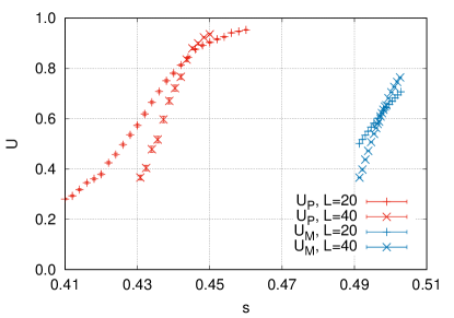
Figure 5: Binder cumulant as a function of $s$ with crossing points for a pair of sizes showing approximate locations of the two transitions at $p=0.95$. (Inset) Extrapolation of crossing points of $(L,2L)$ for $U_{M}$ as a function of $1/L$ fit to the form $f(x)=a+bx$ gives $s_{c}=0.497(1)$.

The $p=0$ limit corresponds to the $K=0$ limit of the AT model and describes decoupled Ising models. The $p=1$ limit has no paramagnetic phase and at some intermediate $p_{\textrm{ Potts}}$ , we would expect $q=4$ Potts criticality. For $p<p_{\textrm{ Pott}s}$, the system would trace out the line of continuously varying exponents and for $1>p>p_{\textrm{ Potts}}$, it would host all three phases along with two Ising transitions; one between the paramagnetic and polarized phases and the other between the polarized and ferromagnetic phases. To investigate these phase transitions, we define a Binder cumulant Binder with coefficients corresponding to $Z_{2}$ symmetry breaking, as

$$U_{M}=\frac{3}{2}\bigg{(}1-\frac{1}{3}\frac{\braket{M^{4}}}{\braket{M^{2}}^{2}}\bigg{)},$$ (6)

where $M$ can denote either $M_{P},M_{\sigma}$ or $M_{\tau}$. In the regime where we have two Ising phase transitions, the Binder cumulant is by this definition zero in the paramagnetic phase and unity in the ordered phase, for whichever order parameter is considered. There is a sharp transition in $U_{M}$ at the phase transition for large sizes and we need to study only one of $M_{\sigma}$ or $M_{\tau}$ as they are identical. By tracking $U_{P}$ (corresponding to $M_{P}$) and $U_{M}$ (corresponding to $M_{\sigma}$), we notice two transitions for $p=0.95$ at distinct values of $s$. This is seen in Fig. 5 through crossing points of the Binder cumulant, and the inset shows an extrapolation of the crossing points of $U_{M}$ as a function of inverse size, which leads to a critical $s$ of $0.497(1)$ separating phases 2 and 3. These two transitions are expected for values of $p$ close to 1 until a point at which the $q=4$ Potts point is realized. The scaling dimension of the spin operator is fixed at $\Delta_{\sigma}=1/8$ (which is the 2D Ising value) along the critical line joining the $p=0$ and $p=p_{\textrm{ Potts}}$, whereas the polarization operator has $\Delta_{P}=\Delta_{\sigma}+\Delta_{\tau}$ at the decoupled point and $\Delta_{P}=\Delta_{\sigma}=\Delta_{\tau}$ at the Potts point. The critical exponent $\nu$ varies from 1 (Ising value) to 3/2 (Potts value) along this line. From our simulations and finite size scaling analysis following the method presented in Ref. Luck, , we observe that, at $p=0.75$, $\nu=1.41(5)$ and $\Delta_{P}=0.13(1)$, indicating that this point is quite close to the Potts point (as can be seen in our approximate phase diagram, Fig. 6). The value of $\nu$ may be somewhat affected by logarithmic corrections expected in the exponents at the Potts point. The same extrapolation at $p=0.50$ gives us $\nu=1.21(1)$ and $\Delta_{P}=0.20(1)$ (the extrapolation for $\Delta_{P}$ is shown in the inset of Fig. 6), which are values between the two extremes. This analysis shows us in a conclusive manner that the system flows to the AT universality class in the thermodynamic limit.

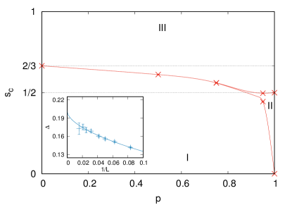
Figure 6: Phase diagram of the model described by Eq. (4) with phases I. paramagnet, II. polarization ordered and III. ferromagnet with the AT line of continuously varying exponents from $p=0$ to $p\approx 0.75$. Inset: Polarization exponent $\Delta_{P}(1/L)$ for $p=0.5$ extrapolated to $\Delta_{P}(0)=0.20(1)$.

IV Relation to Pseudo-first Order Behavior

The Binder cumulant is used in general to identify the nature of a phase transition and the critical exponent $\nu$ for the correlation length (extracted from the slope). Non-monotonic behavior in the Binder cumulant involving a minimum is usually taken as a signature of a first-order transition, although this can only be confirmed by checking that the value of this negative peak diverges as $L^{d}$ Binder . A dip in the Binder cumulant had been misinterpreted to signal a first order transition FOE for the frustrated $J_{1}$-$J_{2}$ classical Ising model on the square lattice where nearest neighbors interact with a ferromagnetic bond of strength $J_{1}$ and next nearest neighbors with an antiferromagnetic bond of strength $J_{2}$ JinSan .In this model there exists a phase transition between a $Z_{4}$ symmetric striped phase and a paramagnetic phase with increasing temperature. The dip was taken to represent a first order transition until a detailed numerical study by Jin et al. JinSan showed that the cumulant dip mapped onto the 2D $q=4$ classical Potts model, which also shows non-monotonicity with a negative dip which does not diverge. The reason for this behavior was traced to the shape of the distribution at the critical point for these models Sannotes and it was noticed that phase coexistence was not seen, which would be a characteristic of a first order transition.

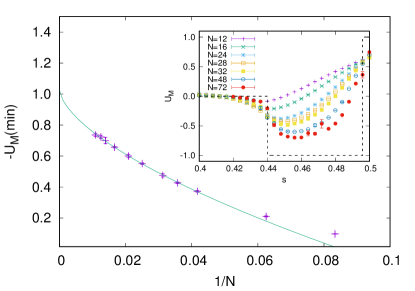
Figure 7: The minimum value of $U_{m}$ for 1D coupled Ising chains, with Hamiltonian given by Eq. (4), at $p=0.95$ as a function of length $L$ fit to the form $a+bL^{-c}$ converges to $1.02(3)$. Inset: $U_{M}$ as a function of tuning parameter $s$ for various system sizes. The thermodynamic from of $U_{M}$ is shown by the dashed line with transitions at 0.44(1) and 0.497(1).

Here we present the same kind of analysis for our model of coupled Ising systems (Eq. (1)) in 1D and argue that the negative peak arises from an inappropriate definition of the Binder cumulant when investigating multiple phase transitions. The Binder cumulant may evaluate to different values in different phases and if the phases are not well understood, this behavior can be interpreted as arising from a first order transition. Even at special points such as the Potts point ($K=1$ point in the AT model), which is known to harbor a continuous phase transition between trivial paramagnetic and ferromagnetic phases, remnants of the polarization ordered phase cause non-monotonic behavior in the Binder cumulant. We will first show the non-monotonic behavior for the coupled Ising chains, and will follow it up by explicitly showing the remnant at the Potts point.

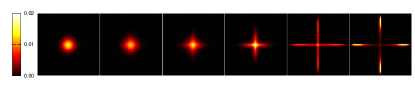
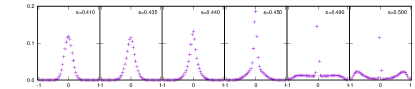
Figure 8: Order parameter histogram as a function of the tuning parameter $s$. Top: The 2D histogram of $M_{x}$ and $M_{y}$. Bottom: Marginal probability distribution of $M_{x}$ at corresponding values of $s$.

If we consider the $p=0.95$ phase transitions presented in the previous sections, we see that in the paramagnetic phase, the Binder cumulant can be defined as

$$U_{M}=2-\frac{\braket{M^{4}}}{\braket{M^{2}}^{2}},$$ (7)

instead of the definition used in Eq. (6), because the magnetization can now be defined as a vector M=$M_{x}\hat{x}+M_{y}\hat{y}$, where $M_{x}(M_{y})$ is the magnetization for the subset of spins with $\sigma^{z}_{i}\tau^{z}_{i}=+1(-1)$. This definition leads to $U_{M}=0$ for the paramagnetic phase and $U_{M}=1$ for the ferromagnetic phase and is used for decoupled Ising systems as well as systems with XY symmetry. Importantly, however, this definition of $U_{M}$ evaluates to $-1$ in the polarization ordered phase as a global value of $\sigma^{z}_{i}\tau^{z}_{i}$ is chosen and only constrained Ising like fluctuations are allowed along this axis forcing $\braket{M^{4}}$/$\braket{M^{2}}^{2}$=3, which can be calculated assuming Gaussian probability distributions arising from the central limit theorem. If we use Eq. (7) for the entire range of $s$ at $p=0.95$, in the thermodynamic limit, we would expect a region where $U_{M}=0$, a region with $U_{M}=-1$ and a region with $U_{M}=1$. A schematic of this is shown in the inset of Fig. 7. For small sizes $U_{M}$ changes gradually and these values are not reached exactly.

From Fig. 5 and extrapolations similar to the one shown in its inset, we note that the paramagnetic to polarization ordered transition occurs at $s=0.44(1)$ and the polarization ordered to ferromagnetic one occurs at $s=0.497(1)$. Following the behavior of $U_{M}$ as defined above, we find a non-monotonicity in the polarized phase where the dip extrapolates to $-1$ (Fig. 7). We also study the histograms of the order parameter M and clearly see the aligning of the polarization in Fig. 8, where we present order parameter histograms for a 50-site system. We observe that the $(M_{x},M_{y})$ histograms look substantially different from a continuous transition as the tails develop a large distributed weight as we cross into the ferromagnetic phase, even though the peak of the histogram is still at $(0,0)$, which represents the disordered phase. This can be seen better in the marginal distribution of $M_{x}$ in the lower panels of Fig. 8, where we see that at $s\approx 0.49$, the histogram shows a spread in weight outside of the disordered region, without a strong peak at the order parameter value for the ordered phase. This behavior is at odds with both a continuous phase transition, where one must have a narrow peak which smoothly moves to $|M_{x}|=1$, and a first order transition, where one must see two narrow peaks in the distribution but is consistent with three phases. In the paramagnetic phase, the fluctuations are Gaussian distributed in a radial pattern, whereas in the polarization ordered phase, they are restricted to one dimensional distributions. In the ferromagnetic phase, the system orders at one of the four peaks.

These histograms are similar to those seen at the Potts point in the $J_{1}$-$J_{2}$ model. We have checked this in the more natural formulation of the classical $q=4$ Potts model on a 2D square lattice, with a Hamiltonian given by

$$H=-\sum_{\langle i,j\rangle}\delta_{q_{i},q_{j}}=-\sum_{\langle i,j\rangle}\cos(\theta_{i}-\theta_{j}),$$ (8)

where $q_{i}\in\{0,1,2,3\}$ are the possible states and which can be represented as unit vectors forming a regular tetrahedron, implying the equivalence of the two terms in Eq. (8) up to a global shift in the baseline for energy. As mentioned above, if the fluctuations in the thermodynamic magnetization are Ising like then $r=\braket{M^{4}}$/$\braket{M^{2}}^{2}=3$ and if they are completely paramagnetic $r=5/3$, which can be seen by evaluating Gaussian integrals over the unit vectors chosen from a tetrahedron and which lie in 3D space. In the ordered phase the fluctuations are small compared to the mean and $r=1$. In the case of a typical continuous transition, $r$ would vary monotonically from 1 to 5/3 from the ordered to paramagnetic phases. This is not the case for the Potts model, as seen from our simulations in Fig. 9, and we find a peak which grows for larger sizes. The peak appears to diverge logarithmically in the range which we have studied, but we would expect this value to converge eventually (perhaps at $r=3$, as shown in the inset of Fig. 9) as we are studying a continuous phase transition. This implies remnant effects of a polarization phase which cannot be explicitly realized in this formulation of the Potts model. These effects persist up to the largest lattice sizes (3072$\times$3072) we were able to study and may be suppressed at even larger scales, in which case the origin of the new length scale would be of interest.

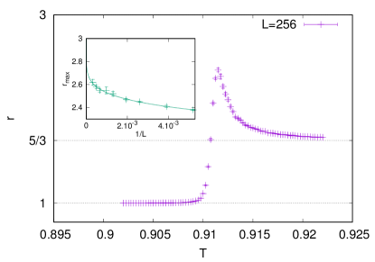
Figure 9: Binder ratio for the 2D $q=4$ Potts model shows a peak at the transition, as shown here for a 256$\times$256 system. Inset: Value of the peak as a function of inverse linear size $1/L$, fit to a function of the from $f(x)=3-ax^{b}$.

V Conclusions

The coupled Ising model discussed here is a tractable system which can source interesting dynamical behavior with excitations showing a restricted extent in space. Due to the intricate structure of non-interacting blocks which this system breaks into, curious features may be manifest in the crossover between quantum and thermal phase transitions, and we intend to study this in future work. Upon the addition of perturbations it is expected that the system regains ergodicity in a manner which depends on the particular perturbation used. There has been a recent numerical study RN which suggests that long time scales persist even in the case of a 1D version of our model in the limit of weak global transverse fields creating a coupling across blocks. In the presence of the same term, we have verified here that the system encodes a quantum realization of the AT model in a Hamiltonian made out of only two body terms explicitly for 1D and expect the same in higher dimensions.

We have also identified a reason for pseudo-first order behavior which is seen in the $q=4$ Potts model in 2D which corresponds to a tricritical point with $q\leq 4$ corresponding to continuous transitions and $q>4$ being first order transitions. This could help explain the microscopic origin of the weak first order transitions in the 1D quantum or 2D classical Potts model, which has been studied from the perspective of complex conformal field theories cCFT1 . By switching off the matrix element of the transverse field in the Potts model which connects odd and even colors, all even color Potts models can be driven to exactly the limit described here. The classical Potts model has also been independently studied in terms of restricted partitions PottsP . Spin liquids with restricted dynamics have already been found to have similar features Sha , and we plan to develop a better understanding for this in analogy with our model in future work.

- (1) T. Senthil, A. Vishwanath, L. Balents, S. Sachdev, and M. P. A. Fisher, Science 303, 1490 (2004).
- (2) A. Nahum, P. Serna, J. T. Chalker, M. Ortuno, and A. M. Somoza, Phys. Rev. Lett. 115, 267203 (2015).
- (3) C. Wang, A. Nahum, M. A. Metlitski, C. Xu, and T. Senthil, Phys. Rev. X 7, 031051 (2017).
- (4) B. Zhao, P. Weinberg, and A. W. Sandvik, Nature Physics 15, 678-682 (2019).
- (5) S. Boixo, Nature Physics 10, 218 (2014).
- (6) E. Farhi, D. Gosset, I. Hen, A. W. Sandvik, P. Shor, A. P. Young, and F. Zamponi, Phys. Rev. A 86, 052334 (2012).
- (7) E. Farhi, J. Goldstone, S. Gutmann, J. Lapan, A. Lundgren, and D. Preda, Science 292, 472 (2001).
- (8) A. A. Belavin, A. M. Polyakov, and A. B. Zamolodchikov, Nucl. Phys. B 241, 333 (1984).
- (9) F. Y. Wu, Rev. Mod. Phys. 54, 235 (1982).
- (10) M. Oshikawa, Phys. Rev. B 61, 3430 (2000).
- (11) R. M. Nandkishore and M. Hermele, Annu. Rev. Condens. Matter Phys. 10, 295 (2019).
- (12) C. Chamon, Phys. Rev. Lett. 94, 040402 (2005).
- (13) P. Sala, T. Rakovszky, R. Verresen, M. Knap, and F. Pollmann, arXiv:1904.04266 (2019).
- (14) V. Khemani and R. Nandkishore, arXiv:1904.04815 (2019).
- (15) O. Sikora, N. Shannon, F. Pollmann, K. Penc, and P. Fulde, Phys. Rev. B 84, 115129 (2011).
- (16) J. Ashkin and E. Teller, Phys. Rev. 64, (5-6): 178-184 (1943).
- (17) J. L. Cardy, J. Phys. A: Math. Gen. 20, 13: L891 (1987).
- (18) G. Delfino and P. Grinza, Nucl. Phys. B 682, 521-550 (2004).
- (19) S. Jin, A. Sen, and A. W. Sandvik, Phys. Rev. Lett. 108, 045702 (2012).
- (20) A. Chandran and C. R. Laumann, Phys. Rev. B 92, 024301 (2015).
- (21) G. E. Andrews, Number Theory (Dover Publications, Philadelphia, 1971).
- (22) C. Sándor, Integers 4, A18 (2004).
- (23) H-O. Heuer, J. Phys. A: Math. Gen. 26, 333 (1993).
- (24) T. Senthil and S. Sachdev, Phys. Rev. Lett. 77, 5292 (1996).
- (25) A. W. Sandvik, Phys. Rev. Lett. 96, 207201 (2006).
- (26) G. H. Hardy, Ramanujan: Twelve Lectures on Subjects Suggested by His Life and Work, 3rd ed. New York: Chelsea (1999).
- (27) A. P. Young and H. Rieger, Phys. Rev. B 53, 8486 (1996).
- (28) M. Suzuki, Comm. Math. Phys. 51, 183 (1976).
- (29) V. Gorbenko, S. Rychkov, and B. Zan, SciPost Phys. 5, 050 (2018).
- (30) A. W. Sandvik, Phys. Rev. B 59, R14157 (1999).
- (31) K. Binder, Z. Phys. B 43, 119 (1981).
- (32) J. M. Luck, Phys. Rev. B 31, 3069 (1985).
- (33) A. Kalz, A. Honecker, and M. Moliner, Phys. Rev. B 84, 174407 (2011).
- (34) A. W. Sandvik, AIP Conference Proceedings 1297, 1 (2010).
- (35) Y. Zhao, R. Narayanan, and J. Cho, arXiv:1906.12020 (2019).
- (36) F. Y. Wu, G. Rollet, H. Y. Huang, J. M. Maillard, C-K. Hu, and C-N. Chen, Phys. Rev. Lett. 76, 173 (1996).
- (37) P. Weinberg and M. Bukov, SciPost Physics 2, 003 (2017).