Double parton distribution of valence quarks in the pion in chiral quark models

Abstract

The valence double parton distribution of the pion is analyzed in the framework of chiral quark models, where in the chiral limit factorization between the longitudinal and transverse degrees of freedom occurs. This feature leads, at the quark-model scale, to a particularly simple distribution of the form $D(x_{1},x_{2},\boldsymbol{q})=\delta(1-x_{1}-x_{2})F(\boldsymbol{q})$, where $x_{1,2}$ are the longitudinal momentum fractions carried the valence quark and antiquark and $\boldsymbol{q}$ is their relative transverse momentum. For $\boldsymbol{q}=\boldsymbol{0}$ this result complies immediately to the Gaunt-Sterling sum rules. The DGLAP evolution to higher scales is carried out in terms of the Mellin moments. We then explore its role on the longitudinal correlation quantified with the ratio of the double distribution to the product of single distributions, $D(x_{1},x_{2},\boldsymbol{q}=\boldsymbol{0})/D(x_{1})D(x_{2})$. We point out that the ratios of moments $\langle x_{1}^{n}x_{2}^{m}\rangle/\langle x_{1}^{n}\rangle\langle x_{2}^{m}\rangle$ are independent of the evolution, providing particularly suitable measures to be tested in the upcoming lattice simulations. The transverse form factor $F(\boldsymbol{q})$ and its Fourier conjugate in the relative transverse coordinate $\boldsymbol{b}$ are obtained in variants of the Nambu–Jona-Lasinio model with the spectral and Pauli-Villars regularizations. The results are valid in the soft-momentum domain. Interestingly, with the spectral regularization of the model, the effective cross section for the double parton scattering of pions is exactly equal to the geometric cross section, $\sigma_{\rm eff}=\pi\langle\boldsymbol{b}^{2}\rangle$ and yields about 20 mb.

I Introduction 

The pion, which according to the constituent quark model is composed of a quark $q$ and antiquark $\bar{q}$ pair, enjoys being the would-be Goldstone boson of the spontaneously broken chiral symmetry – a feature which explains its particularly low mass as compared to other hadrons. There exist many observables which probe indirectly the consequences of the pion being both a pseudo-Goldstone boson and a composite $q\bar{q}$ state, indicating its extended non-elementary structure at intermediate energies. These include the electromagnetic and gravitational form factors (FF), transition form factors, electromagnetic polarizabilities, as well as features of their the mutual interactions, such as the Gasser-Leutwyler coefficients. Likewise, for high-energy processes where hard-soft factorization holds, the soft matrix elements within the pion state yield the single parton distribution functions (sPDF), the corresponding generalized parton distributions (GPD), transverse momentum distributions (TMD), parton distribution amplitudes (PDA), etc.

A strong motivation to investigate the double parton distribution functions (dPDFs) in the pion comes from the more and more promising prospects of the lattice QCD studies Bali et al. (2018); Zimmermann (2016). In this paper we address the valence dPDF of the pion in the simplest covariant field-theoretic approach to its structure, namely the Nambu–Jona-Lasinio (NJL) model Nambu and Jona-Lasinio (1961a, b), where the pion arises as a Goldstone boson of the spontaneously broken chiral symmetry and as a $q\bar{q}$ relativistic bound state of the Bethe-Salpeter equation. This model is not renormalizable and needs a suitable regularization. Here we use the Pauli-Villars (PV) regularization which preserves chiral symmetry and gauge invariance Schuren et al. (1992) (for a review see, e.g., Ruiz Arriola (2002)). We also explore the Spectral Quark Model (SQM) Ruiz Arriola (2001); Ruiz Arriola and Broniowski (2003), where particularly simple analytic formulas can obtained.

The story of dPDFs is rather old Kuti and Weisskopf (1971), with first experimental traces of the possible double parton scattering (DPS) in multi-jet events in $pp$ collisions reported by the Axial Field Spectrometer Collaboration at the CERN ISR Akesson et al. (1987) and in $p\bar{p}$ collisions by the CDF Collaboration at Fermilab Abe et al. (1993, 1997). With a renewed interest in the LHC era, several enlightening theoretical works (see Bartalini et al. (2011); Snigirev (2011); Luszczak et al. (2012); Manohar and Waalewijn (2012a, b) and references therein) preceded the measurement of $W$ production in association with two jets by the ATLAS Collaboration Aad et al. (2013), which provided a strong case for the need of DPS. Thereby dPDFs have become more directly accessible to experimental scrutiny and quantitative analysis (for reviews see, e.g., d’Enterria and Snigirev (2013) for implications in production processes). For a recent state of affairs see Bartalini and Gaunt (2018).

As any partonic quantity, dPDFs are scale dependent and their evolution is dictated by a generalized form of the DGLAP equations Kirschner (1979); Shelest et al. (1982), where gluon radiation is explicitly implemented. In the case of the pion, the correlation structure is particularly relevant, as it indicates to what extent the quark and anti-quark are entangled in the presence of additional gluons. While it will be hard to measure dPDF for the pion experimentally, some of its features will become soon available from lattice QCD Bali et al. (2018); Zimmermann (2016), thus offering a unique chance of testing the internal structure of the pion and, more specifically, the correlations between its $q\bar{q}$ constituents. However, the quest for dPDFs is non-perturbative, whereas the evolution only relates these quantities perturbatively at different scales, saying nothing about their absolute determination at a given scale. Hence the importance of non-perturbative modeling.

Similarly to the previous studies of sPDFs, we assume that there exists a reference scale $\mu_{0}$ where the pion is just a $q\bar{q}$ state. This is suggested by the observation that the momentum fraction carried by the quarks at the scale $\mu=4~{}{\rm GeV}$ is about $42-44\%$ Sutton et al. (1992); Gluck et al. (1999) and that it increases according to LO and NLO DGLAP evolution with decreasing $\mu$. Then at about $\mu_{0}\sim 320~{}{\rm MeV}$ the valence quark and antiquark carry all the momentum. While this is admittedly a low scale, it has been checked that switching from LO to NLO evolution in model calculations does not change more than $10\%$ the pion sPDFs Davidson and Ruiz Arriola (2002), justifying the approach.

Chiral quark models offer a view of the pion as a relativistic $q\bar{q}$ Goldstone boson, departing from the naive quark model. One of the important features of these models is that they are constructed to satisfy the gauge invariance and the chiral Ward-Takahashi identities. This is important to recover the current algebra results at low energies and to guarantee proper normalization of form factors and PDFs. Moreover, the imposition of relativity via the Bethe-Salpeter equation implements proper support for partonic quantities. Despite these strong constraints, there is still freedom in enforcing proper regularization schemes. In this paper we focus for definiteness on the NJL model with the PV regularization Schuren et al. (1992); Ruiz Arriola (2002) for which sPDFs Davidson and Ruiz Arriola (1995), TMDs Weigel et al. (1999), PDAs Ruiz Arriola and Broniowski (2002), GPDs Broniowski et al. (2008) have been computed. We also explore the SQM, which is particularly simple in the resulting formulas and offers a qualitatively good description both at low and at higher energies Ruiz Arriola and Broniowski (2003); Ruiz Arriola and Broniowski (2003); Megias et al. (2004). These variants of the NJL model have been used in the past to describe the FF, PDFs, PDAs, GPDs, TMDs, comparing favorably both to experimental data as well as available lattice results.

After some of the results presented here were advertised Broniowski and Ruiz Arriola (2019), a relevant preprint by Courtoy, Noguera, and Scoppeta has been released Courtoy et al. (2019), addressing in a comprehensive way the dPDF calculation in the NJL model. Our results confirm closely the basic findings Courtoy et al. (2019), despite different regularization schemes. Here we also fully present the results of the QCD evolution for dPDF and discuss in detail the issue of the longitudinal partonic correlation.

It is worth noting some other non-perturbative studies of dPDFs in quark models for the nucleon, such as in the MIT bag Chang et al. (2013) or in the constituent quark model model Rinaldi et al. (2013), also with the light-front wave functions Rinaldi et al. (2014, 2018). We stress that the longitudinal correlation features in these models are qualitatively understood in the framework of the valon model Hwa and Zahir (1981); Hwa and Yang (2002), as shown in Broniowski and Ruiz Arriola (2014); Broniowski et al. (2016).

The paper is organized as follows. After introducing the definitions and our notation in Sec. II, we present the NJL model and the calculation of the valence dPDF of the pion in Sec. III. A recurrent issue in this kind of calculations regards the interplay between regularization and positivity, a topic which we address in Section IV. The QCD DGLAP evolution and the corresponding matching condition for the model are discussed in Sec. V, with numerical results presented in Sec. VI. In Sec. VII we present ratios of moments of dPDF to product of moments of sPDFs, which are scale independent for the valence distributions. These ratios could most directly be tested in lattice calculations. The transverse form factor depends somewhat on the variant of the model, as shown in Sec. VIII, where also a few related observables of interest are evaluated and discussed. Finally, in Sec. IX we come to our summary.

II Basic definitions and properties

In this section we list for completeness (and to establish our notation) the basic definitions. The spin-averaged sPDF and dPDF (see Diehl (2010) and references therein) of a hadron with momentum $p$ involve forward matrix elements of parton bilinear operators, namely

$$D_{j_{1}}(x_{1})=\int\frac{dz^{-}}{2\pi}\,e^{ix_{1}z^{-}p^{+}}\langle p|\,{\mathcal{O}_{j_{1}}(0,z)}\,|p\rangle\bigl{|}_{z^{+}=0\,,\boldsymbol{z}=\boldsymbol{0}},$$

$$D_{j_{1}j_{2}}(x_{1},x_{2},\boldsymbol{b})=2p^{+}\int dy^{-}\,\frac{dz^{-}_{1}}{2\pi}\,\frac{dz^{-}_{2}}{2\pi}\;e^{i(x_{1}z_{1}^{-}+x_{2}z_{2}^{-})p^{+}}$$

$$\times\langle p|\,{\mathcal{O}_{j_{1}}(y,z_{1})\,\mathcal{O}_{j_{2}}(0,z_{2})}\,|p\rangle\bigl{|}_{z_{1}^{+}=z_{2}^{+}=y_{\phantom{1}}^{+}=0\,,\boldsymbol{z}_{1}=\boldsymbol{z}_{2}=\boldsymbol{0}},$$

(1)

with $j_{1,2}$ indicating the parton species, the bold face denoting the transverse vectors, and $\boldsymbol{b}$ playing the role of the transverse distance between the two partons, with $y=(y^{+},y^{-},\boldsymbol{b})$. The light-cone coordinates are defined as $a^{\pm}=(a^{0}\pm a^{3})/\sqrt{2}$. The longitudinal (i.e., ⁺) momentum fractions carried by the partons are denoted customarily as $x_{1}$ and $x_{2}$.

For the quarks and antiquarks, considered in this paper, the bilocal color-singlet operators are

$$\mathcal{O}_{q}(y,z)=\tfrac{1}{2}\,\bar{q}(y-\tfrac{z}{2})\gamma^{+}W(y-\tfrac{z}{2},y+\tfrac{z}{2})q(y+\tfrac{z}{2}),$$

$$\mathcal{O}_{\bar{q}}(y,z)=-\tfrac{1}{2}\,\bar{q}(y+\tfrac{z}{2})\gamma^{+}W(y+\tfrac{z}{2},y-\tfrac{z}{2})q(y-\tfrac{z}{2}),$$

where the summation over color is implicit and the flavor indices are omitted for brevity. As the quark and antiquark coordinates in the individual operators $\mathcal{O}_{j}$ in Eq. (1) are not split in the transverse direction, the light-front gauge $A^{-}_{a}=0$ along straight line paths eliminates the Wilson gauge link operators $W$, setting them to identity (the splitting in $\boldsymbol{b}$ occurs between the color singlet bilinears, which is innocuous). Thus the complications in maintaining the gauge invariance and the choice of the Wilson line, encumbering TMDs Collins (2011) and the corresponding QCD evolution Vladimirov (2015); Echevarria et al. (2016) (for a review see, e.g.,  Scimemi (2019) and references therein), do not occur in the case of dPDFs.

One may pass to the momentum representation via the Fourier transform

$$D_{j_{1}j_{2}}(x_{1},x_{2},\boldsymbol{q})=\int d^{2}\boldsymbol{b}\,e^{i\boldsymbol{b}\cdot\boldsymbol{q}}D_{j_{1}j_{2}}(x_{1},x_{2},\boldsymbol{b}),$$ (3)

where the same symbol $D$ is used, with the argument distinguishing the function from its transform. The double distributions for the case where $\boldsymbol{q}=\boldsymbol{0}$, denoted for brevity as

$$D_{j_{1}j_{2}}(x_{1},x_{2})=D_{j_{1}j_{2}}(x_{1},x_{2},\boldsymbol{q}=\boldsymbol{0})$$ (4)

acquire a special significance, as they satisfy the Gaunt-Stirling (GS) sum rules Gaunt and Stirling (2010). These identities follow straightforwardly Gaunt (0 09) when the decomposition of the parton operators in a basis of the light-front wave functions is made, and are essentially statements on completeness of the Fock states as well as flavor and longitudinal momentum conservation. The sum rules read

$$\sum_{i}\int_{0}^{1-x_{2}}\!\!\!dx_{1}\,x_{1}D_{ij}(x_{1},x_{2})=(1-x_{2})D_{j}(x_{2}),$$

$$\int_{0}^{1-x_{2}}\!\!\!\!\!\!\!\!dx_{1}\,D_{i_{\rm val}j}(x_{1},x_{2})=(N_{i_{\rm val}}\!-\!\delta_{ij}\!+\!\delta_{\bar{i}j})D_{j}(x_{2}),$$ (5)

where $i_{\rm val}$ indicates the difference of the parton ($i$) and antiparton ($\bar{i}$) distributions, and

$$N_{i_{\rm val}}=\int_{0}^{1}dx\,D_{i_{\rm val}}(x).$$ (6)

To satisfy the GS sum rules, we have argued in Broniowski and Ruiz Arriola (2014); Broniowski et al. (2016) that a practical approach is the top-down method, where one starts with $n$-body parton distributions with the longitudinal momentum fractions constrained with $\delta(1-x_{1}-...-x_{n})$, and subsequently generates distributions with a lower number of partons via marginal projections. This avoids complications of bottom-up attempts in constructing dPDFs from known sPDFs, which cannot be unique and where one encounters problems Gaunt and Stirling (2010); Golec-Biernat and Lewandowska (2014). Also, note a recent study Diehl et al. (2019) devoted to a verification of the GS sum rules in covariant perturbation theory and in light-cone perturbation theory.

The above discussion presumes a probabilistic interpretation of dPDFs, similarly to sPDFs. As has been known, however (see, e.g., Kasemets and Mulders (2015)), the need for renormalization of the bare definitions (1) may in principle invalidate positivity, as it inherently involves subtraction. The issue is subtle, as violation of positivity precludes a probabilistic interpretation. Moreover, it should also be recalled that the QCD evolution equations (see Sec. V below) do not preserve positivity; whereas the DGLAP evolution produces positive distributions when evolving upward from $Q_{0}$ to $Q>Q_{0}$, for downward evolution, $Q<Q_{0}$, the positivity property may actually be violated Llewellyn Smith and Wolfram (1978) (mostly at small $x$). For an explicit nucleon study and a practical distinction between the (scheme dependent) positivity of parton distributions and the necessary positivity of physically measurable cross sections, we refer the reader to Ruiz Arriola (1998). The generation of negative components with downward evolution is also a feature of the dPDF evolution equations applied here.

Secondly, there is a question of retaining positivity at nonzero $\boldsymbol{b}$, or a corresponding Fourier conjugate momentum $\boldsymbol{q}$. The mentioned derivation of the GS sum rules for $\boldsymbol{q}=\boldsymbol{0}$ via the Fock-state decomposition involves a summation of moduli squared of the $n$-parton wave functions, $|\phi_{n}(\{\boldsymbol{k}_{i}\},\{x_{i}\})|^{2}$, which is positive and may remain so upon certain renormalization procedures, e.g., the Fock space truncation. With $\boldsymbol{q}\neq\boldsymbol{0}$, the corresponding terms involve ${\rm Re}\left[\phi_{n}(\{\boldsymbol{k}_{i}\},\{x_{i}\})\phi_{n}^{\ast}(\{\boldsymbol{k}_{i}+\boldsymbol{q}_{i}\},\{x_{i}\})\right]$, which mathematically need not be positive definite, as the wave functions may possess nodes. Of course, in processes where hard-soft factorization holds, thus where the dPDFs are useful, the pertinent cross sections must obviously be positive, which constitutes the true positivity constraints. The issue of positivity is further discussed in Sec. IV.

We note that the factorization of the longitudinal and transverse degrees of freedom,

$$D_{j_{1}j_{2}}(x_{1},x_{2},\boldsymbol{q})=D_{j_{1}j_{2}}(x_{1},x_{2})F_{j_{1}j_{2}}(\boldsymbol{q}),$$ (7)

has been a standard working assumption in studies of DPS over the recent years, which so far finds support from dynamical model calculations Chang et al. (2013); Rinaldi et al. (2013). We remark that in this case the positivity property can be considered separately for $D_{j_{1}j_{2}}(x_{1},x_{2})$ and for the form factor $F_{j_{1}j_{2}}(\boldsymbol{q})$.

We end this section with remarks concerning the lattice QCD results of Bali et al. (2018); Zimmermann (2016) in the context of our studies. There, the basic object is the correlation function, which bares some similarity to the dPDF definition (1), but also carries relevant differences. Firstly, typical of the lattice simulations, the currents are local, with $z_{1}^{-}$ and $z_{2}^{-}$ set to zero, which corresponds to the integration over $x_{1}$ and $x_{2}$. Second, the relative time difference of the two currents in Bali et al. (2018); Zimmermann (2016) is set to zero, whereas in Eq. (1) integration over $y^{-}$ is carried out. To focus more precisely on this issue, let us denote the relevant matrix element in terms of Lorentz invariants,

$$\langle p|\,{\mathcal{O}_{j_{1}}(y,0)\,\mathcal{O}_{j_{2}}(0,0)}\,|p\rangle=f_{j_{1}j_{2}}(p\cdot y,y^{2}).$$ (8)

In the light cone kinematics of Eq. (1) $p\cdot y=p^{+}y^{-}$, $y^{2}=-\boldsymbol{b}^{2}$, and integration over $p\cdot y$ is carried out. In the instant form of the lattice studies $p\cdot y=p^{0}y^{0}$, $y^{2}=-\boldsymbol{y}^{2}$, and $p\cdot y=0$. If, instead of integration over $y^{-}$ in Eq. (1) we set $y^{-}=0$, the Lorenz covariance would immediately link the two approaches. Since it is not so, the transverse form factors from dPDFs and the lattice evaluations are different objects. For that reason the transverse form factors related to dPDFs discussed in Sec. VIII cannot be directly compared to the results presented in Bali et al. (2018); Zimmermann (2016). A model interpretation of the interesting lattice data requires a separate study which should also incorporate in addition the corresponding finite pion mass, typically $\sim 300$ MeV, used in those simulations.

III The model

Figure 1: The diagram for the chiral quark model evaluation of the valence dPDF of $\pi^{+}$. The loop consists of the constituent quark propagators. The blobs indicate the probing operators $\gamma^{+}$, and the pseudoscalar quark-pion coupling $i\gamma_{5}$. The integration over $\int dk_{-}\int d^{2}k_{\perp}\int dq_{-}$ enforces the kinematic constraints of the definition (1).

The large-$N_{c}$ evaluation in chiral quark models amounts to evaluating one-quark-loop integrals. For definiteness, we consider the positively charged pion $\pi^{+}$, with other states related by the isospin symmetry. The relevant diagram for the valence dPDF in the momentum representation is shown in Fig. 1, where the loop momentum integration is constrained with $k^{+}=x_{1}p^{+}$, as we assign $x_{1}$ as the longitudinal momentum fraction carried by the valence $u$ quark. Note that with just two constituents this constraint simultaneously fixes the longitudinal momentum carried by the valence antiquark $\bar{d}$ to be $x_{2}=1-x_{1}$. With the Feynman quark propagator

$$S_{k}=\frac{i}{\not{k}-M+i\epsilon},$$ (9)

where $M$ is the constituent quark mass due to the spontaneous breaking of the chiral symmetry, the diagram of Fig. 1 reads

$$D_{u\bar{d}}(x_{1},x_{2},\boldsymbol{q})=\delta(1-x_{1}-x_{2})\frac{M^{2}}{f^{2}}\int\frac{d^{4}k}{(2\pi)^{4}}\int\frac{dq^{-}}{2\pi}\times$$

$$\delta(k^{+}-x_{1}p^{+}){\rm Tr}\left[\gamma^{+}S_{k}\gamma^{5}S_{k-p}\gamma^{+}S_{k-p}\gamma_{5}S_{k}\right],$$ (10)

where the trace is over color and Dirac indices. We use the pseudoscalar quark-pion coupling $M/f\times i\gamma_{5}$, where $f=86$ MeV is the pion decay constant in the chiral limit. An explicit and straightforward evaluation yields Broniowski and Ruiz Arriola (2019); Courtoy et al. (2019)

$$D_{u\bar{d}}(x_{1},x_{2},\boldsymbol{q})=\delta(1-x_{1}-x_{2})\theta(x_{1})\theta(1-x_{1})F(\boldsymbol{q}),$$

(11)

with the form factor

$$\vspace{-10mm}F(\boldsymbol{q})=\left.\frac{N_{c}M^{2}}{(2\pi)^{3}f^{2}}\int d^{2}\boldsymbol{k}\frac{\boldsymbol{k}\cdot(\boldsymbol{k}+\boldsymbol{q})+M^{2}}{(\boldsymbol{k}^{2}+M^{2})((\boldsymbol{k}+\boldsymbol{q})^{2}+M^{2})}\right|_{\rm reg.},$$

(12)

which is ultraviolet log-divergent and needs to be properly regularized, as indicated.

For $\boldsymbol{q}=\boldsymbol{0}$, upon regularization, the integral reduces to

$$F(0)=\left.\frac{N_{c}M^{2}}{(2\pi)^{3}f^{2}}\int d^{2}\boldsymbol{k}\frac{1}{\boldsymbol{k}^{2}+M^{2}}\right|_{\rm reg.},$$ (13)

which is equal to 1, as follows from a corresponding expression for the square of the pion decay constant $f^{2}$ (cf. for instance Broniowski et al. (2008)). Then

$$D_{u\bar{d}}(x_{1},x_{2},\boldsymbol{q})=\delta(1-x_{1}-x_{2})\theta(x_{1})\theta(1-x_{1}),$$ (14)

the result advocated in Broniowski and Ruiz Arriola (2019); Courtoy et al. (2019).

As shown in Courtoy et al. (2019), other large-$N_{c}$ diagrams, which formally appear in the effective quark-meson model, do not contribute to $D_{u\bar{d}}$.

Thus, at the quark model scale $\mu_{0}$, the double parton distribution of the pion takes a product form of the individual longitudinal momentum fractions carried by each valence quark, multiplied by $\delta(1-x_{1}-x_{2})$, coming from the momentum conservation and the fact that at the quark model scale the only constituents in the pion are the two valence partons.

We recall that for the valence sPDF the corresponding result is Davidson and Ruiz Arriola (1995)

$$D_{\rm val}(x)=\theta(x)\theta(1-x).$$ (15)

Taking into account the fact that our model result factorize according to Eq. (11), we discuss separately the longitudinal and transverse structures in the following sections.

IV Regularization vs positivity

In this section we address some technical aspects concerning the interplay between the necessary finite cut-off regularization in a chiral quark model and the positivity which proves the basis for the insightful probabilistic interpretation. As already mentioned, even in QCD this is a subtle issue Kasemets and Mulders (2015). To simplify the discussion, in this section we assume sharp cut-offs either in coordinate or momentum space. Generally, these schemes encounter difficulties with gauge invariance. More sophisticated (smooth but gauge invariant) schemes are worked out in Sec. VIII.

On a formal level, it is noteworthy that Eq. (12) has a convolution-like structure that can be rewritten in the form

$$F(\boldsymbol{q}) = \frac{N_{c}M^{2}}{(2\pi)^{3}f^{2}}\int d^{2}\boldsymbol{k}_{1}d^{2}\boldsymbol{k}_{2}\delta(\boldsymbol{k_{1}}-\boldsymbol{k_{2}}+\boldsymbol{q})$$ (16)

$$\times \left[\Psi(\boldsymbol{k_{1}})\boldsymbol{k_{1}}\cdot\Psi(\boldsymbol{k_{2}})\boldsymbol{k_{2}}+M^{2}\Psi(\boldsymbol{k_{1}})\Psi(\boldsymbol{k_{2}})\right],$$

where

$$\Psi(\boldsymbol{k})=\frac{1}{\sqrt{\boldsymbol{k}^{2}+M^{2}}}.$$ (17)

Formally, we may pass to the coordinate space by defining

$$\Phi(\boldsymbol{b})=\int\frac{d^{2}\boldsymbol{k}}{(2\pi)^{2}}\Psi(\boldsymbol{k})e^{i\boldsymbol{k}\cdot\boldsymbol{b}}=\frac{e^{-bM}}{2\pi b},$$ (18)

with $\boldsymbol{b}$ the two-dimensional transverse coordinate. From here we get

$$F(\boldsymbol{q})=\frac{N_{c}M^{2}}{2\pi f^{2}}\int d^{2}\boldsymbol{b}\,e^{i\boldsymbol{b}\boldsymbol{q}}\left[\nabla\Phi(\boldsymbol{b})^{2}+M^{2}\Phi(\boldsymbol{b})^{2}\right],$$ (19)

such that the form factor appears as the Fourier transform of a manifestly positive function in $b$-space. In our case $\Phi(\boldsymbol{b})\sim e^{-Mb}/b$, hence the integral diverges at small distances. If we put a short distance transverse cut-off, it is not guaranteed that the form factor in momentum space remains positive. In fact, if we impose the normalization condition, $F(0)=1$, we get a short distance cut-off $b_{0}\sim 0.5~{}{\rm fm}$ and the form factor presents a multinodal structure with alternating signs, the first zero curring at $|\boldsymbol{q}|\sim 0.75~{}{\rm MeV}$.

Alternatively, since the formula for $F(\boldsymbol{q})$ is divergent, a regularization must be imposed. A simple method within momentum space would be to use a purely transverse cut-off $\Lambda_{\perp}$ and fix it according to the normalization condition given by Eq. (13). This is the essence of the light front regularization method applied in Ref. Courtoy et al. (2019), which, requires additional assumptions to be compatible with soft physics and, in particular, to provide a non-vanishing vacuum quark condensate (see e.g. Dietmaier et al. (1989); Heinzl (2001)). Such a prescription, however, does not preserve positivity Courtoy et al. (2019).

An interesting aspect is that, as noted in Weigel et al. (1999) (see Appendix A for an analysis in the case of the pion em form factor), usual convolution formulas, as the one discussed above, are only formally correct but not necessarily compatible with gauge invariance or chiral symmetry.

The above discussion shows once again that implementation of a finite cut-off regularization in chiral quark models is a nontrivial issue, particularly if a finite regularization is imposed separately on the individual Feynman diagrams. The effective action method suggested by Eguchi Eguchi (1976) is a symmetry preserving scheme which allows for a proper discussion of chiral symmetry breaking even after the implementation of a regularization method Schuren et al. (1992); Ruiz Arriola (2002) and provides a common regularization for all diagrams involving pions, photons, or W and Z bosons. Therefore, here we only consider regularization methods which comply with soft pion physics and chiral symmetry, but then they need not preserve positivity of the dPDF form factor away from the soft limit (particularly above the finite cut-off). Thus, chiral quark models are designed to describe soft physics, whereas large $|\boldsymbol{q}|$, or small $b$, evade this requirement, even after regularization, which we encounter below.

V Evolution and matching

Parton distribution functions describe non-perturbative properties of a hadron, namely its quark and gluon content, as functions of their longitudinal momentum fraction. These quantities depend on the renormalization scale, which usually is taken to be $\mu=Q$, a typical momentum appearing in the experimental process. Their running with the scale $\mu$ follows from the invariance of the physical cross sections. The evolution can only be implemented perturbatively, thus a non-perturbative input is required at a reference scale $\mu_{0}$ to provide initial conditions for the pertinent evolution equations.

Phenomenological analyses of the pion parameterize the valence, sea, and gluon sPDFs at relatively large scales, $\mu\sim 2~{}{\rm GeV}$ Sutton et al. (1992), or intermediate scales $\mu\sim 0.5~{}{\rm GeV}$ Gluck et al. (1999), with the result that at $\mu\sim 2~{}{\rm GeV}$ the momentum fraction carried by the quarks in the pion is $0.42-0.44$. In fact, in a hadronic model such as NJL applied here, one only has valence quarks and antiquarks, hence it makes sense to fix $\mu_{0}$ by imposing that these constituents saturate the momentum sum rule, $\langle x\rangle_{\mu_{0}}=1$. This provides a hadronic scale of $\mu_{0}\sim 320~{}{\rm MeV}$ (see, e.g., Broniowski et al. (2016)), which we refer to as the quark model scale. Once the reference scale $\mu_{0}$ is fixed, the matching condition between the model and QCD observables is imposed by

$$\left.A(x,\mu_{0})\right|_{\rm model}=\left.A(x,\mu_{0})\right|_{\rm QCD}.$$ (20)

The QCD evolution equations for multi-parton distributions have been derived long ago Kirschner (1979); Shelest et al. (1982). A simple and numerically efficient method is based on the Mellin moments, similarly to the case of sPDFs (for results of a practical implementation see, e.g., Broniowski and Ruiz Arriola (2014) for the nucleon and Broniowski et al. (2016) for the pion).

While for ease of notation we do not write explicitly the $\boldsymbol{b}$ dependence, the evolution equations quoted below are still valid for that case Diehl et al. (2014). Clearly, for a factorized ansatz, the transverse dependence also factorizes out from the evolution. As we have discussed in the previous section, this is actually the case in chiral quark models in the chiral limit.

One introduces the moments of the sPDFs and dPDFs,

$$M^{n}_{j}=\int_{0}^{1}dx\,x^{n}D_{j}(x),$$ (21)

$$M^{n_{1}n_{2}}_{j_{1}j_{2}}=\int_{0}^{1}\!\!dx_{1}\int_{0}^{1}\!\!dx_{2}\theta(1\!-\!x_{1}\!-\!x_{2})x_{1}^{n_{1}}x_{2}^{n_{2}}D_{j_{1}j_{2}}(x_{1},x_{2}),$$

and the moments of the QCD splitting functions

$$P_{i\to j}^{n}=\int_{0}^{1}dx\,x^{n}P_{i\to j}(x),$$ (22)

$$P_{i\to j_{1}j_{2}}^{n_{1}n_{2}}=\int_{0}^{1}dx\,x^{n_{1}}(1-x)^{n_{2}}P_{i\to j_{1}j_{2}}(x),$$

$${\tilde{P}}_{i\to j_{1}j_{2}}^{n_{1}n_{2}}=\delta_{j_{1}j_{2}}P_{i\to j_{1}}^{n_{1}+n_{2}}-\delta_{ij_{1}}P_{j_{1}\to j_{2}}^{n_{2}}-\delta_{ij_{2}}P_{j_{2}\to j_{1}}^{n_{1}}.$$

Then the DGLAP evolution equations are Kirschner (1979); Shelest et al. (1982) (for simplicity, the possible two scales $\mu_{1}$ and $\mu_{2}$ for the two operators are set to be equal to a single scale $\mu$)

$$\frac{d}{dt}M^{n_{1}n_{2}}_{j_{1}j_{2}}=\sum_{i}P_{i\to j_{1}}^{n_{1}}M^{n_{1}n_{2}}_{ij_{2}}+\sum_{i}P_{i\to j_{2}}^{n_{2}}M^{n_{1}n_{2}}_{j_{1}i}$$

$$~{}~{}~{}+\sum_{i}\left(P_{i\to j_{1}j_{2}}^{n_{1}n_{2}}+{\tilde{P}}_{i\to j_{1}j_{2}}^{n_{1}n_{2}}\right)M^{n_{1}+n_{2}}_{i},$$ (23)

where

$$t=\frac{1}{2\pi\beta}\log\left[1+\alpha_{s}(\mu)\beta\log(\Lambda_{\rm QCD}/\mu)\right],$$ (24)

$$\beta=\frac{11N_{c}-2N_{f}}{12\pi}.$$ (25)

Partons $i$, $j_{1}$, and $j_{2}$ may in general represent the valence quarks/antiquarks, the sea, or the gluons, whose distributions are coupled. Moreover, the last term in Eq. (23) couples dPDFs to sPDFs, serving as an inhomogeneous term. The evolution acquires a simpler form when one probes just the valence quarks, which is the case considered in this work, where we take $\pi^{+}$ with $j_{1}=u$ and $j_{2}=\bar{d}$. In that case there are no partons $i$ contributing to the splitting $P_{i\to j_{1}j_{2}}$, and the inhomogeneous term vanishes. In addition, the nonsiglet valence quarks do not mix with the singlet component (sea quarks and gluons), leaving for the considered $\pi^{+}$ state the equation

$$\frac{d}{dt}M^{n_{1}n_{2}}_{u\bar{d}}(t)=\left(P_{u\to u}^{n_{1}}+P_{\bar{d}\to\bar{d}}^{n_{2}}\right)M^{n_{1}n_{2}}_{u\bar{d}}(t).$$ (26)

Figure 2 represents a typical diagram for the applied evolution in terms of the developing parton cascades along the $t$-channel.

Figure 2: A typical QCD diagram corresponding to the evolution (26) of the valence dPDF of $\pi^{+}$. The dots correspond to insertions of $\gamma^{+}$.

VI Numerical results of evolution

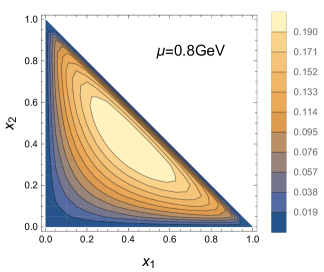
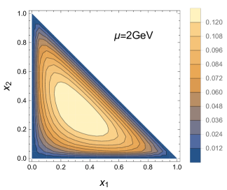
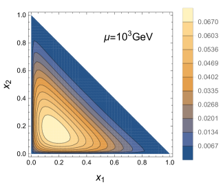
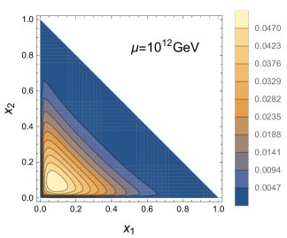
Figure 3: The valence dPDF of $\pi^{+}$ evolved with the DGLAP equations to subsequent scales of $\mu=0.5$, $2$, $10$, $1000$, and $10^{9}$ GeV. The dimensionless quantity plotted is $x_{1}x_{2}D(x_{1},x_{2};\mu)$. The initial condition at $\mu=\mu_{0}$ is the singular distribution of Eq. (14).

The DGLAP evolution described above in an obvious manner preserves the longitudinal-transverse factorization, as all moments are multiplied conventionally with $F(\boldsymbol{q})$. For that reason we may discuss the evolution of $D_{\rm u\bar{d}}(x_{1},x_{2})$.

It is known that the DGLAP evolution preserves the GS sum rules Gaunt and Stirling (2010). In our case, the sum rules are trivially satisfied at the quark model scale $\mu_{0}$, as with Eqs. (11) and (15) one immediately gets

$$\int_{0}^{1-x_{2}}dx_{1}D_{\rm u\bar{d}}(x_{1},x_{2})=D_{\bar{d}}(x_{2}),$$

$$\int_{0}^{1-x_{1}}dx_{2}D_{\rm u\bar{d}}(x_{1},x_{2})=D_{{u}}(x_{1}),$$

$$\int_{0}^{1-x_{2}}dx_{1}x_{1}D_{\rm u\bar{d}}(x_{1},x_{2})=(1-x_{2})D_{\bar{d}}(x_{2}),$$

$$\int_{0}^{1-x_{1}}dx_{2}x_{2}D_{\rm u\bar{d}}(x_{1},x_{2})=(1-x_{1})D_{{u}}(x_{1}).$$ (27)

Thus the GS sum rules are satisfied at any scale.

Our numerical results for the evolution of the valence dPDF of the pion (multiplied with $x_{1}x_{2}$) are presented in Fig. 3, where we show it for increasing evolution scale $\mu$. We note the gradual drift towards the asymptotic fixed point $\delta(x_{1})\delta(x_{2})$.

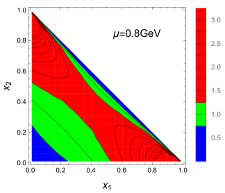
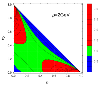
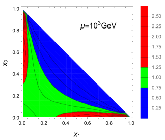
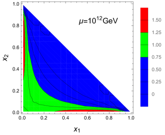
Figure 4: Correlation $D_{\rm u\bar{d}}(x_{1},x_{2})/D_{u}(x_{1})D_{\bar{d}}(x_{2})$ at various evolution scales $\mu$.

The longitudinal correlations can be conveniently quantified with the ratio $D_{\rm u\bar{d}}(x_{1},x_{2})/D_{u}(x_{1})D_{\bar{d}}(x_{2})$, which would be equal to 1 if no correlations were present. Our results for this measure are shown in Fig. 4. We note that for large scales $\mu$ and simultaneously low $x_{1}$ and $x_{2}$ (which is where dPDF is large) the correlation ratio is within a 20% band around unity, hence there the effect is not very substantial, justifying the product ansatz for dPDF. The largest effect occurs for asymmetric kinematics, with $x_{1}$ large and $x_{2}$ small, or vice versa, where correlations are strong and positive. The explanation of this behavior is related to the overall conservation of the longitudinal momentum. The qualitative argument here is that at large $\mu$, with many partons present, the constraint of the longitudinal momentum is effective only when one of the considered partons takes a large momentum fraction, thus leaving significantly less of available phase space for the other parton. We remark that a qualitatively similar effect has been found for gluodynamics in Golec-Biernat et al. (2015); Golec-Biernat and Stasto (2017); Elias et al. (2018).

VII Ratios of moments

The LO DGLAP evolution of the valence moments, due to the absence of the inhomogeneous term, leads to a simple fact that the ratios $\langle x_{1}^{n}x_{2}^{m}\rangle/\langle x_{1}^{n}\rangle\langle x_{2}^{m}\rangle$ for the valence distributions do not depend on the evolution scale, as the evolution ratio factors with the anomalous dimensions cancel out. More explicitly, the evolution for the valence moments reads

$$M_{n}(\mu)=\left(\frac{\alpha(\mu)}{\alpha(\mu_{0})}\right)^{\gamma_{n}/2\beta_{0}}M_{n}(\mu_{0}),$$

$$M_{nm}(\mu)=\left(\frac{\alpha(\mu)}{\alpha(\mu_{0})}\right)^{\gamma_{n}/2\beta_{0}+\gamma_{m}/2\beta_{0}}M_{nm}(\mu_{0}),$$ (28)

with $\gamma_{i}$ denoting the anomalous dimensions, thus the cancellation is obvious. Despite its simplicity, this feature is rather remarkable, as it allows for an insight into lower scales, where non-pertubative dynamics sets in, from the information at higher scales.

In particular, in the NJL model we immediately find the following scale independent ratios:

$$\frac{\langle x_{1}^{n}x_{2}^{m}\rangle}{\langle x_{1}^{n}\rangle\langle x_{2}^{m}\rangle}=\frac{(1+n)!(1+m)!}{(1+n+m)!}.$$ (29)

The first few ratios are shown in Table 1. The largest ratio is for $m=n=1$. Naturally, the moments are the quantities to be probed with the upcoming lattice studies and it is interesting to see if the pattern of Eq. (29) holds. The pattern of the moments is specific to a given (non-perturbative) model, allowing for its scrutiny provided the lattice data would be accurate enough.

Table 1: The NJL model ratios of the valence moments $\langle x_{1}^{n}x_{2}^{m}\rangle/\langle x_{1}^{n}\rangle\langle x_{2}^{m}\rangle$ from Eq. (29). Rows and columns correspond to $n$ and $m$.

	1	2	3	4	5
1	$\tfrac{2}{3}$	$\tfrac{1}{2}$	$\tfrac{2}{5}$	$\tfrac{1}{3}$	$\tfrac{2}{7}$
2	$\tfrac{1}{2}$	$\tfrac{3}{10}$	$\tfrac{1}{5}$	$\tfrac{1}{7}$	$\tfrac{3}{28}$
3	$\tfrac{2}{5}$	$\tfrac{1}{5}$	$\tfrac{4}{35}$	$\tfrac{1}{14}$	$\tfrac{1}{21}$
4	$\tfrac{1}{3}$	$\tfrac{1}{7}$	$\tfrac{1}{14}$	$\tfrac{5}{126}$	$\tfrac{1}{42}$
5	$\tfrac{2}{7}$	$\tfrac{3}{28}$	$\tfrac{1}{21}$	$\tfrac{1}{42}$	$\tfrac{1}{77}$

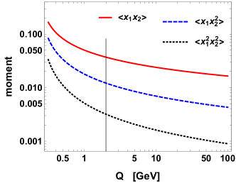
Figure 5: Lowest moments of the valence dPDF of the pion as a function of the renormalization scale according to LO DGLAP evolution.

The LO DGLAP evolution of the lowest moments of the valence dPDF of the pion is displayed in Fig. 5. We note a fall-off from the quark model scale controlled by the corresponding anomalous dimensions in Eq. (28).

VIII Transverse structure

The NJL model needs to be regularized to get rid of the ultraviolet divergences, leaving only the soft-momentum degrees of freedom in the dynamics. Unlike the longitudinal structure, the transverse structure depends specifically on the regularization. This is a subtle issue, since as already discussed, the chiral and gauge symmetries must be preserved by the regularization procedure, as has been discussed at length in Schuren et al. (1992) (for a review see, e.g., Ruiz Arriola (2002)). We give here the final recipes as applied to the unregularized result of Eq. (12), both for the PV and SQM implementations. We present first the SQM results, as the final formulas are particularly simple in this case.

VIII.1 Spectral Quark Model

In the SQM, one replaces the constituent quark mass $M$ in Eq. (12) with a spectral mass, $w$, and integrates over $w$ with a spectral weight,

$$A(M)|_{\rm SQM}=\int_{C}dw\rho(w)A(w)$$ (30)

over a suitably chosen complex contour $C$ Ruiz Arriola and Broniowski (2003). One may adjust $\rho(w)$ and $C$ in such a way that the construction implements an exact vector-meson dominance principle of the pion electromagnetic form factor, namely $F_{\rm em}(Q^{2})=1/(1+Q^{2}/m_{\rho}^{2})$, with $m_{\rho}^{2}=24\pi^{2}f^{2}/N_{c}$, yielding $m_{\rho}=764~{}{\rm MeV}$ at $f=86$ MeV in the chiral limit. In this scheme, the normalization condition is $\int_{C}dw\rho(w)=1$.

After computing the spectral integral as well as the $\boldsymbol{k}$ integral, the form factor is given by a very simple formula

$$F(\boldsymbol{q})=\frac{m_{\rho}^{4}-\boldsymbol{q}^{2}m_{\rho}^{2}}{\left(m_{\rho}^{2}+\boldsymbol{q}^{2}\right){}^{2}},$$ (31)

which is a combination of the dipole (with positive sign) and monopole (with negative sign) form factors. The form factor $F(\boldsymbol{q})$ is correctly normalized at $\boldsymbol{q}=0$, namely $F(0)=1$, and vanishes as ${\cal O}(|\boldsymbol{q}|^{-2})$ for large $|\boldsymbol{q}|$.

In Fig 6(a) we show the form factor $F(\boldsymbol{q})$ for SQM (solid line). As we can see, in accordance with Eq. (31), this function becomes negative for $|\boldsymbol{q}|>m_{\rho}$. Thus the result does nor obey positivity (cf. the discussion at the end of Sec. II). Passing to the configuration space via the Fourier-Bessel transform we get

$$f(b) = \int\frac{d^{2}\boldsymbol{q}}{(2\pi)^{2}}e^{i\boldsymbol{b}\cdot\boldsymbol{q}}F(\boldsymbol{q})$$ (32)

$$= \frac{m_{\rho}^{2}}{2\pi}\left[bm_{\rho}K_{1}\left(bm_{\rho}\right)-K_{0}\left(bm_{\rho}\right)\right],$$

with $K_{n}(x)$ denoting the modified Bessel functions of order $n$.

The form factor combination $bf(b)$ for SQM is is depicted in Fig 6(b) with a solid line. By definition, this function is normalized to unity, $\int d^{2}bf(b)=1$, and the corresponding mean squared radius (msr) is given by

$$\langle b^{2}\rangle_{\rm dPDF}=\int d^{2}b\,b^{2}f(b)=\frac{12}{m_{\rho}^{2}}=(0.88~{}{\rm fm})^{2}.$$ (33)

This radius is a 2D quantity in relative parton-parton transverse coordinates, and naively one expects a geometric relation to the 3D radius, which would yield $\langle r^{2}\rangle=\tfrac{3}{2}\langle b^{2}\rangle=(1.07~{}{\rm fm})^{2}$. It is interesting to compare this measure with another msr regarding the hadron size, for instance the electromagnetic (em) msr, which in SQM is given by $\langle r^{2}\rangle_{\rm em}=6/m_{\rho}^{2}=\tfrac{1}{2}\langle b^{2}\rangle_{\rm dPF}=(0.62~{}{\rm fm}^{2})$. Thus, in this model the transverse size (a 2D object) is about $\sqrt{2}$ larger than the em msr (a 3D object). At large distances $f(b)$ behaves as

$$f(b)=\frac{\sqrt{b}\,m_{\rho}^{5/2}e^{-bm_{\rho}}}{2\sqrt{2\pi}}\left[1+{\cal O}\left(\frac{1}{m_{\rho}b}\right)\right],$$ (34)

which falls off exponentially with the mass $m_{\rho}$, which in a constituent picture is typically $m_{\rho}\simeq 2M$ corresponding to a double parton property, opposite to the $m_{\rho}/2\simeq M$ scales in single parton properties Ruiz Arriola and Broniowski (2003).

At short distances $f(b)$ becomes negative and divergent, since

$$f(b)=\frac{m_{\rho}^{2}}{2\pi}\left[\log(\tfrac{1}{2}bm_{\rho})+\gamma+1\right]+O\left(b^{2}\right),$$ (35)

where $\gamma=0.5772\dots$ is the Euler-Mascheroni constant. Using this asymptotics we get a zero of the function $f(b)$ for the value $b_{0}\sim 2e^{-1-\gamma}/m_{\rho}\sim 0.1~{}{\rm fm}$. In Fig. 6(b) we show the $b-$dependence and, as we can see, the function becomes negative at $b\sim 0.15~{}{\rm fm}$, which by the way is comparable to the current day spacing of fine QCD lattices, $a\sim 0.1~{}{\rm fm}$.

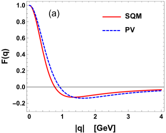
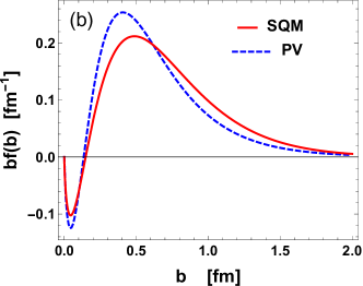
Figure 6: Valence dPDF form factor of the pion in the Spectral Quark Model (solid lines) and in NJL with PV regularization (dashed lines), plotted as functions of the transverse momentum (a) and the transverse coordinate (b), in the combination $bf(b)$.

The effective cross section for DPS is a phenomenologically important quantity Del Fabbro and Treleani (2001), defined as

$$\sigma_{\rm eff}=\frac{1}{\int\frac{d^{2}\boldsymbol{q}}{(2\pi)^{2}}F(\boldsymbol{q})F(-\boldsymbol{q})}.$$ (36)

For SQM we get

$$\sigma_{\rm eff}=\pi\frac{12}{m_{\rho}^{2}}=\pi\langle b^{2}\rangle_{\rm dPDF}=23~{}{\rm mb},$$ (37)

which coincides exactly with the geometric cross section (see the discussion in Rinaldi et al. (2013)). This number is somewhat larger from similar estimates for the nucleon case, where one obtains about 15 mb (see for instance Blok et al. (2012); Traini et al. (2017); Blok et al. (2014))

Actually, if we restricted the integration limit to the value where the effective form factor $f(b)$ is positive, we would get about twice the value for the effective cross section, 47 mb.

Within this context there exists a nested bound for $\sigma_{\rm eff}$, found recently by Rinaldi and Ceccopieri Rinaldi and Ceccopieri (2018), namely $\pi\langle b^{2}\rangle\leq\sigma_{\rm eff}\leq 3\pi\langle b^{2}\rangle$. The derivation of these interesting inequalities rests on the positivity of $f(b)$ (such that $\langle b^{n}\rangle\geq\langle b\rangle^{n}$). The lower bound is saturated by a monopole (which is positive) as well as our solution (which becomes negative for $|\boldsymbol{q}|\geq m_{\rho}$ or for $b\lesssim 0.5/m_{\rho}$). To compare, a dipole yields $\sigma_{\rm eff}=\tfrac{3}{2}\pi\langle b^{2}\rangle$, and a Gaussian profile gives $\sigma_{\rm eff}=2\pi\langle b^{2}\rangle$.

VIII.2 NJL with Pauli-Villars regularization

The most straightforward regularization scheme satisfying the necessary formal requirements is PV regularization with two subtractions in the coincidence limit Schuren et al. (1992), where the one-quark-loop quantity $A(M^{2})$ is replaced with

$$A(M^{2})|_{\rm reg,PV} \equiv A(M^{2})-A(M^{2}\!+\!\Lambda^{2})$$ (38)

$$+ \Lambda^{2}\frac{d}{d\Lambda^{2}}A(M^{2}\!+\!\Lambda^{2}).$$

A detailed analysis shows that the rule is only applied to the mass dependence under the integral in Eq. (12), but not to the $M^{2}$ factor in front, originating from the coupling constant. The normalization yields the well-known condition

$$1 = \frac{N_{c}M^{2}}{(2\pi)^{3}f^{2}}\int d^{2}\boldsymbol{k}\frac{1}{\boldsymbol{k}^{2}+M^{2}}\Big{|}_{\rm reg}$$ (39)

$$= \frac{N_{c}M^{2}}{4\pi^{2}f^{2}}\left[\log\frac{M^{2}+\Lambda^{2}}{M^{2}}+\frac{\Lambda^{2}}{\Lambda^{2}+M^{2}}\right],$$

linking the constituent quark mass and the PV cutoff $\Lambda$ at a given value of $f$. Following earlier works, we take $M=300~{}{\rm MeV}$ and $f=86~{}{\rm MeV}$ in the chiral limit, which fixes the PV cut-off to be $\Lambda=731~{}{\rm MeV}$. The expression for the valence dPDF form factor is

$$F(\boldsymbol{q}) = \frac{M^{2}N_{c}}{4\pi^{2}f^{2}}\Big{[}-\log(M^{2})+\frac{|\boldsymbol{q}|}{\sqrt{4M^{2}+\boldsymbol{q}^{2}}}$$ (40)

$$\times \log\left(\frac{\sqrt{4M^{2}+\boldsymbol{q}^{2}}-|\boldsymbol{q}|}{\sqrt{4M^{2}+\boldsymbol{q}^{2}}+|\boldsymbol{q}|}\right)\Big{]}\Big{|}_{\rm reg.}.$$

Its asymptotic behavior is similar to SQM. Moreover, the msr is given by

$$\langle b^{2}\rangle=\frac{N_{c}\Lambda^{4}}{2\pi^{2}f^{2}\left(M^{2}+\Lambda^{2}\right)^{2}}=(0.77~{}{\rm fm)^{2}}$$ (41)

and the effective cross section is numerically close to the geometric one, $\sigma_{\rm eff}\sim\pi\langle b^{2}\rangle$. The corresponding form factors in the momentum and configuration spaces can also be seen in Fig. 6 (dashed lines). As we can appreciate, they are very similar to the SQM case, including negative values at high momenta $\sim 1~{}{\rm GeV}$ or, equivalently, at short transverse distances $b\lesssim 0.1~{}{\rm fm}$.

IX Conclusions

We have presented a detailed study of the valence double parton distributions in the pion in chiral quark models, with the following basic results:

• The model leads in the chiral limit to a factorization of the longitudinal and transverse structure of the valence pion dPDF, in accordance to the findings of Broniowski and Ruiz Arriola (2019); Courtoy et al. (2019). At the quark model scale, the longitudinal distribution is of the simple form $\delta(1-x_{1}-x_{2})$, reflecting the momentum conservation with just two constituents.

• The LO DGLAP evolution is carried out in the Mellin space, leading to radiative generation of partons at higher scales, and resulting with distributions at higher scales, accessible in experiments or lattice simulations.

• The Gaunt-Stirling sum rules are explicitly satisfied in our approach.

• The longitudinal correlations, quantified as the departure of dPDF from the product of two sPDFs, are studied in detail. An assessment of the validity of the frequently used product ansatz is made, with the result that at high evolution scales and small momentum fractions of both constituents it works to a good approximation.

• Simple expressions are obtained for the transverse form factor of the valence dPDF in the applied regularizations of the chiral quark models. The issue of regularization and positivity is discussed.

• Specific ratios of moments of valence dPDF to product of moments of valence sPDFs follow from the applied model. Such quantities, invariant of the evolution scale, may be used with future lattice data to scrutinize non-perturbative models of the pion structure.