A dynamically load-balanced parallel $p$-adaptive implicit high-order flux reconstruction method for under-resolved turbulence simulation

Abstract

We present a dynamically load-balanced parallel $p$-adaptive implicit high-order flux reconstruction method for under-resolved turbulence simulation. The high-order explicit first stage, singly diagonal implicit Runge–Kutta (ESDIRK) method is employed to circumvent the restriction on the time step size. The pseudo transient continuation is coupled with the matrix-free restarted generalized minimal residual (GMRES) method to solve the nonlinear equations at each stage, except the first one, of ESDIRK. We use the spectral decay smoothness indicator as the refinement/coarsening indicator for $p$-adaptation. A dynamic load balancing technique is developed with the aid of the open-source library ParMETIS. The trivial cost, compared to implicit time stepping, of mesh repartitioning and data redistribution enables us to conduct $p$-adaptation and load balancing every time step. An isentropic vortex propagation case is employed to study the impact of element weights used in mesh repartitioning on parallel efficiency. We apply the $p$-adaptive solver for implicit large eddy simulation (ILES) of the transitional flows over a cylinder when Reynolds number (Re) is $3900$ and the SD7003 wing when Re is $60000$. Numerical experiments demonstrate that a significant reduction in the run time (up to 70%) and total number of solution points (up to 76%) can be achieved with $p$-adaptation.

Keywords

Dynamic load balancing; dynamic $p$-adaptation; implicit large eddy simulation; implicit high-order flux reconstruction; matrix-free GMRES.

1 Introduction

Recent decades have witnessed tremendous developments in high-order computational fluid dynamics (CFD) methods, such as discontinuous Galerkin methods (DG) [1, 2, 3, 4, 5, 6, 7, 8], spectral difference methods (SD) [9, 10, 11, 12], classic compact finite difference methods [13, 14], finite difference summation by parts (SBP) operators [15, 16, 17], and flux reconstruction/correction procedure via reconstruction methods (FR/CPR) [18, 19, 20, 21, 22, 23, 24]. Low-dissipation and low-dispersion properties of high-order methods have made them attractive for implicit large eddy simulation (ILES) of turbulent flows. It has been reported in [25] that DG-based ILES can outperform subgrid-model-based LES for transitional flows and wall bounded flows. The dissipation of high-order methods on low-frequency large-scale flow features is trivial, and it is only significant on high wavenumbers/frequencies. Therefore, the truncation error of high-order methods is considered as an implicit subgrid model for turbulence simulation. We note that high-order methods are prone to suffer from instabilities due to aliasing errors in under-resolved turbulence simulation, especially when the spatial polynomial degree exceeds two. It has been shown that with proper de-aliasing techniques, ILES using high-order methods has promising capabilities in under-resolved turbulence simulation [7]. Four popular types of stabilization approaches for under-resolved turbulence simulation can be found in the literature, including (a) the split form [26, 27], (b) over integration [28, 29], (c) artificial viscosity via spectral vanishing viscosity [30, 31, 32], and (d) polynomial filtering [33, 34, 35]. In this study, we employ nodal polynomial filtering proposed by Fisher and Mullen [35] when de-aliasing is needed.

A uniformly high-order spatial discretization in the entire flow field for under-resolved turbulence simulation of certain problems, such as wall bounded turbulent flows at high Reynolds numbers, is very expensive. As a matter of fact, the high-order spatial discretization is only needed in the near wall region, such as the turbulent boundary layer, and the wake region where vortex shedding dominates. Collocation schemes favor a straightforward implementation of $p$-adaption, which has the potential to significantly decrease computational cost. In the literature, three major groups of adaptation methodologies can be found. The first one is the feature-based adaptation [36, 37, 38], the second one is the truncation-error-based or discretization-error-based adaptation [39, 40, 41], and the last one is the output-based or adjoint-based adaptation [42, 43, 44, 45]. Feature-based adaptation methods are usually ad hoc and heavily rely on empirical parameters; however, their ease of implementation and reasonable robustness make them a good choice for adaptation. Truncation-error based approaches usually use the correction from either an additional coarser mesh or a lower-order discretization to estimate the local discretization error, which can serve as the adaptation indicator. A comparison of several feature-based and discretization-error-based adaptation indicators is conducted by Naddei et al. [38]. Adjoint-based adaptation methods are popular for engineering purposes since engineers are more interested in output functionals, such as, lift and drag. Their superiority over the former two approaches has been demonstrated for steady problems. However, the computational cost of adjoint-based adaptation, especially for unsteady turbulence simulation, can be large. Recently, Bassi et al. [46] employed an efficient entropy-adjoint-based [47] $p$-adaptive DG solver to conduct scale-resolving turbulence simulation. In this study, we will evaluate the performance of a feature-based adaptation method [38], which employs the spectral decay smoothness indicator [48] as the refinement/coarsening indicator when it is applied to under-resolved turbulence simulation.

Explicit high-order Runge-Kutta (RK) methods [49, 50] have been widely applied to unsteady flow simulation. $p$-adaptation will naturally lead to $p$-enrichment in near wall regions where the elements are usually clustered, thus worsening the Courant–Friedrichs–Lewy (CFL) condition when explicit methods are employed. Implicit time integrators can essentially circumvent the CFL restriction that explicit methods have. Diagonally implicit RK methods [51] and backward differentiation formula (BDF) methods are among the most popular implicit time integration methods. Recently, linearly implicit Rosenbrock methods have become popular for under-resolved turbulence simulation [52, 53]. Matrix-based implicit methods are notorious for the large memory consumption. Therefore, the matrix-free implementation [53, 54] is usually employed to reduce memory usage [55] for massive turbulence simulation. Though Rosenbrock methods can be potentially more efficient than ESDIRK methods [53], we employ ESDIRK methods in this study since they are more robust than Rosenbrock methods in the context of matrix-free implementation with an element-Jacobi preconditioner.

Given that the time step size of an implicit time integrator can be relatively large, dynamic adaptivity is desired to track the rapid change of turbulence features. Consequently, the work loads on all processes in parallel simulation will be imbalanced once $p$-adaptation takes place. The difference of numbers of degrees of freedom on different processes can be over 500% for a simple isentropic vortex propagation problem [56]. Hence, a dynamic load balancing technique is of crucial importance for the parallel efficiency of $p$-adaptive methods. Existing publications regarding $p$-adaptive high-order methods for turbulence simulation use the mean flow field to conduct the adaptation without dynamic adaptivity [37, 46]. We utilize the open-source library ParMETIS [57] to achieve dynamic load balancing for $p$-adaptation. Technical details on using ParMETIS for dynamic adaptivity are presented in Section 3 for interested readers. In our numerical experiments, we find that the cost of mesh repartitioning and data redistribution is trivial compared to that of implicit time stepping, which enables the $p$-adaptation to be conducted every time step to significantly decrease the run time.

Contributions. We develop a dynamically load balanced $p$-adaptation technique for parallel implicit high-order flux reconstruction solution of unsteady Navier–Stokes equations. The implementation regarding the dynamic load balancing technique is presented in detail. We discuss the impact of weight calculation for each element on the parallel efficiency of $p$-adaptation when implicit time integrators are used. The $p$-adaptive solver is applied to under-resolved turbulence simulation of the transitional flow over an infinite cylinder at $\text{Re}=3900$ and the transitional flow over the SD7003 wing at $\text{Re}=60000$. Compared to the $p$-uniform spatial discretization, the $p$-adaptive FR method can save up to $70\%$ computational cost when $p\leq 3$ in our experiments and provide favorable numerical predictions. We expect more savings when $p$ is higher as demonstrated in a simple experiment of the isentropic vortex propagation problem.

Organization. The remainder of the paper is organized as follows. Section 2 provides the mathematical background of the governing equations, the spatial discretization, and the time integration. Section 3 introduces the $p$-adaptation algorithm with the spectral decay smoothness indicator, and then explains the parallel mesh partitioning technique with ParMETIS. A simple example is employed to demonstrate the impact of weight calculation of each element on the parallel efficiency. Applications of the $p$-adaptive solver to under-resolved turbulence simulation are presented in Section 4. In Section 5, we draw conclusions from the current work.

2 Background

2.1 Governing equations

Using Einstein summation convention, the compressible Navier–Stokes equations can be written as

$$\frac{\partial\rho}{\partial t}+\frac{\partial(\rho u_{j})}{\partial x_{j}}=0,$$ (1)

$$\frac{\partial(\rho u_{i})}{\partial t}+\frac{\partial(\rho u_{j}u_{i}+\delta_{ji}p)}{\partial x_{j}}=\frac{\partial\tau_{ji}}{\partial x_{j}},$$ (2)

$$\frac{\partial(\rho E)}{\partial t}+\frac{\partial(\rho u_{j}H)}{\partial x_{j}}=\frac{\partial(u_{i}\tau_{ij}-K_{j})}{\partial x_{j}},$$ (3)

where $i=1,\dots,n_{d}$, and $n_{d}$ is the dimension number. Herein, $\rho$ is the fluid density, $u_{i}$ is the velocity component, $p$ is the pressure, $E=\frac{p/\rho}{\gamma-1}+\frac{1}{2}u_{k}u_{k}$ is the specific total energy, $H=E+\frac{p}{\rho}$ is the specific total enthalpy, $\tau_{ij}$ is the viscous stress and $K_{j}$ is the heat flux. Note that only in this section, $p$ refers to pressure; in other sections, $p$ stands for polynomial degree. $\gamma$ is the specific heat ratio defined as $\gamma=C_{p}/C_{v}$, where $C_{p}$ and $C_{v}$ are specific heat capacity at constant pressure and volume, respectively. In this study, $\gamma$ is set as 1.4. The ideal gas law $p=\rho RT$ holds, where $R$ is the ideal gas constant and $T$ is the temperature. The viscous stress tensor and heat flux vector are given by

$$\tau_{ij}=2\mu\left\{S_{ij}-\frac{1}{3}\frac{\partial u_{k}}{\partial x_{k}}\delta_{ij}\right\},$$ (4)

$$K_{j}=-\frac{\mu C_{p}}{\text{Pr}}\frac{\partial T}{\partial x_{j}},$$ (5)

where $\mu$ is the fluid dynamic viscosity, Pr is the molecular Prandtl number, and the strain-rate tensor $S_{ij}$ is defined as

$$S_{ij}=\frac{1}{2}\left(\frac{\partial u_{i}}{\partial x_{j}}+\frac{\partial u_{j}}{\partial x_{i}}\right).$$ (6)

In this study, $\mu$ and Pr are treated as constants.

2.2 The FR/CPR method

For completeness, a brief review of the FR/CPR method [20] is presented in this section. A symbolic form of the compressible Navier–Stokes equations (1), (2), (3) is written as

$$\frac{\partial\boldsymbol{q}}{\partial t}+\nabla\cdot\boldsymbol{f}=0,$$ (7)

which is defined in domain $\Omega$. $\Omega$ is partitioned into $N$ non-overlapping and conforming elements $\Omega_{e}$, where $e=0,1,\ldots,N-1$. After multiplying each side by the test function $\boldsymbol{\vartheta}$ and integrate over $\Omega_{e}$, one obtains

$$\int_{\Omega_{e}}\frac{\partial\boldsymbol{q}_{e}}{\partial t}\,\boldsymbol{\vartheta}\,dV+\int_{\Omega_{e}}\boldsymbol{\vartheta}\,\nabla\cdot\boldsymbol{f}_{e}\,dV=0.$$ (8)

On applying the integration by parts and divergence theorem, Eq. (8) reads

$$\int_{\Omega_{e}}\frac{\partial\boldsymbol{q}_{e}}{\partial t}\,\boldsymbol{\vartheta}\,dV+\int_{\partial\Omega_{e}}\boldsymbol{\vartheta}\,\boldsymbol{f}_{e}\cdot\boldsymbol{n}\,dS-\int_{\Omega_{e}}\boldsymbol{f}_{e}\cdot\nabla\boldsymbol{\vartheta}\,dV=0,$$ (9)

where $\boldsymbol{n}$ is the outward-facing unit normal vector of the faces of the element $\Omega_{e}$. In the discrete form, we assume $\boldsymbol{q}_{e}^{h}$ is the approximate solution in element $\Omega_{e}$. The solution and the test function belong to the polynomial space of degree $k$, i.e., $\boldsymbol{q}_{e}^{h}\in p^{k}$ and $\boldsymbol{\vartheta}^{h}\in p^{k}$. To ensure conservation, $\boldsymbol{f}_{e}\cdot\boldsymbol{n}$ in Eq. (9) is replaced with $\boldsymbol{f}^{com}_{\boldsymbol{n}}$, the common flux in the normal direction of the element surfaces. Eq. (9) then reads

$$\int_{\Omega_{e}}\frac{\partial\boldsymbol{q}_{e}^{h}}{\partial t}\,\boldsymbol{\vartheta}^{h}\,dV+\int_{\partial\Omega_{e}}\boldsymbol{\vartheta}^{h}\,\boldsymbol{f}^{com}_{\boldsymbol{n}}\,dS-\int_{\Omega_{k}}\boldsymbol{f}_{e}^{h}\cdot\nabla\boldsymbol{\vartheta}^{h}\,dV=0.$$ (10)

After applying integration by parts and divergence theorem again to the last term of Eq. (10), one obtains

$$\int_{\Omega_{e}}\frac{\partial\boldsymbol{q}_{e}^{h}}{\partial t}\,\boldsymbol{\vartheta}^{h}\,dV+\int_{\Omega_{e}}\boldsymbol{\vartheta}^{h}\,\nabla\cdot\boldsymbol{f}_{e}^{h}\,dV+\int_{\partial\Omega_{e}}\boldsymbol{\vartheta}^{h}\,[\boldsymbol{f}]\,dS=0,$$ (11)

where $[\boldsymbol{f}]=\boldsymbol{f}^{com}_{\boldsymbol{n}}-\boldsymbol{f}^{loc}_{\boldsymbol{n}}$ with $\boldsymbol{f}^{loc}_{\boldsymbol{n}}=\boldsymbol{f}_{e}^{h}\cdot\boldsymbol{n}$. In the FR/CPR method, the correction field $\boldsymbol{\delta}_{e}\in p^{k}$ is defined as [20]

$$\int_{\partial\Omega_{e}}\boldsymbol{\vartheta}^{h}\,[\boldsymbol{f}]\,dS=\int_{\Omega_{e}}\boldsymbol{\vartheta}^{h}\,\boldsymbol{\delta}_{e}\,dV.$$ (12)

Therefore, Eq. (11) can be expressed as

$$\int_{\Omega_{e}}\left(\frac{\partial\boldsymbol{q}_{e}^{h}}{\partial t}+\nabla\cdot\boldsymbol{f}_{e}^{h}+\boldsymbol{\delta}_{e}\right)\,\boldsymbol{\vartheta}^{h}\,dV=0.$$ (13)

The differential form can then be employed as

$$\frac{\partial\boldsymbol{q}_{e}^{h}}{\partial t}+\mathbb{P}\left(\nabla\cdot\boldsymbol{f}_{e}^{h}\right)+\boldsymbol{\delta}_{e}=0.$$ (14)

Herein, $\mathbb{P}\left(\nabla\cdot\boldsymbol{f}_{e}^{h}\right)$ is the projection of the flux divergence $\left(\nabla\cdot\boldsymbol{f}_{e}^{h}\right)$, which may not be a polynomial, onto an appropriate polynomial space. We note that Eq. (14) can be directly derived from the differential form; their equivalence has been established in [58]. Specifically, for quadrilateral and hexahedral elements, the correction field can be obtained by means of the tensor product of the one dimensional correction polynomials; for triangular and tetrahedral elements, the readers are referred to [20, 59]. Only hexahedral elements are considered in this study.

The Roe approximate Riemann solver [60] is used to calculate the common inviscid fluxes at the cell interfaces in their normal directions as

$$\boldsymbol{f}_{\boldsymbol{n},inv}^{com}=\frac{\boldsymbol{f}_{\boldsymbol{n},inv}^{+}+\boldsymbol{f}_{\boldsymbol{n},inv}^{-}}{2}-\boldsymbol{R}|\boldsymbol{\varLambda}|\boldsymbol{R}^{-1}\frac{\boldsymbol{q}^{+}-\boldsymbol{q}^{-}}{2},$$ (15)

where superscripts ‘$-$’ and ‘$+$’ denote the left of right side of the current interface, the subscript $\boldsymbol{n}$ is the unit normal direction from left to right, $\boldsymbol{\varLambda}$ is a diagonal matrix consisting of the eigenvalues of the preconditioned Jacobian $\partial\boldsymbol{f}_{\boldsymbol{n}}/\partial\boldsymbol{q}$, and $\boldsymbol{R}$ consists of the corresponding right eigenvectors evaluated with the averaged values. The common viscous fluxes at the cell interfaces are $\boldsymbol{f}_{n,vis}^{com}=\boldsymbol{f}_{vis}(\boldsymbol{q}^{+},\nabla\boldsymbol{q}^{+},\boldsymbol{q}^{-},\nabla\boldsymbol{q}^{-})$. Here, we need to define the common solution $\boldsymbol{q}^{com}$ and common gradient $\nabla\boldsymbol{q}^{com}$ at the cell interface. On simply taking average of the primitive variables, we get

$$\boldsymbol{q}^{com}=\frac{\boldsymbol{q}^{+}+\boldsymbol{q}^{-}}{2}.$$ (16)

The common gradient is computed as

$$\nabla\boldsymbol{q}^{com}=\frac{\nabla\boldsymbol{q}^{+}+\boldsymbol{r}^{+}+\nabla\boldsymbol{q}^{-}+\boldsymbol{r}^{-}}{2},$$ (17)

where $\boldsymbol{r}^{+}$ and $\boldsymbol{r}^{-}$ are the corrections to the gradients on the interface. The second approach of Bassi and Rebay (BR2) [5] is used to calculate the corrections.

2.3 ESDIRK methods with pseudo transient continuation

The ESDIRK methods for the 3D compressible Navier-Stokes equation (7) can be written as

$$\begin{cases}\boldsymbol{q}^{n+1}=\boldsymbol{q}^{n}+\Delta t\,\sum_{i=1}^{s}b_{i}\boldsymbol{R}(\boldsymbol{q}^{i}),\\ \boldsymbol{q}^{i}=\boldsymbol{q}^{n},i=1,\\ \boldsymbol{q}^{i}=\Delta t\,\omega\,\boldsymbol{R}(\boldsymbol{q}^{i})+\boldsymbol{q}^{n}+\Delta t\,\sum_{j=1}^{i-1}a_{ij}\boldsymbol{R}(\boldsymbol{q}^{j}),i=2,\dots,s,\end{cases}$$ (18)

where $i$ is the stage number, $s$ is number of total stages, $n$ denotes the physical time step, and $\boldsymbol{R}=-\nabla\cdot\boldsymbol{f}$. The second-order, three-stage ESDIRK2 [51], and fourth-order, six-stage ESDIRK4 [61] methods are employed in this paper. A comparative study of different implicit time integration methods can be found in [53]. In every stage except the first one, a nonlinear system is to be solved, which can be expressed as

$$\boldsymbol{F}(\boldsymbol{q}^{i})=\left(-\frac{1}{\omega\,\Delta t}\boldsymbol{q}^{i}+\boldsymbol{R}(\boldsymbol{q}^{i})\right)+\frac{1}{\omega\,\Delta t}\left(\boldsymbol{q}^{n}+\Delta t\sum_{j=1}^{i-1}a_{ij}\boldsymbol{R}(\boldsymbol{q}^{j})\right),\,i=2,\dots,s.$$ (19)

The pseudo transient continuation for the $i$-th stage reads

$$\frac{\boldsymbol{q}^{m+1,i}-\boldsymbol{q}^{m,i}}{\Delta\tau}=\boldsymbol{F}(\boldsymbol{q}^{m+1,i}),$$ (20)

where $m$ is the iteration step. Eq. (20) can be linearized as

$$\left(\frac{1}{\omega\,\Delta t}+\frac{1}{\Delta\tau}-\frac{\partial\boldsymbol{R}}{\partial\boldsymbol{q}}\right)^{m}\Delta\boldsymbol{q}^{m,i}=\boldsymbol{F}(\boldsymbol{q}^{m,i}),$$ (21)

where $\Delta\boldsymbol{q}^{m,i}=\boldsymbol{q}^{m+1,i}-\boldsymbol{q}^{m,i}$. We employ the successive evolution relaxation (SER) algorithm [62] to update the pseudo time step size as

$$\Delta\tau^{0}=\Delta\tau_{init},\ \text{and}\ \Delta\tau^{m+1}=\min\left(\Delta\tau^{m}\frac{||\boldsymbol{F}||_{L_{2}}^{m-1}}{||\boldsymbol{F}||_{L_{2}}^{m}},\Delta\tau_{max}\right).$$ (22)

In all the numerical experiments conducted in this study, we set the convergence tolerance of relative residual of the pseudo transient continuation as $tol_{rel}^{pseudo}=10^{-4}$.

We use the restarted GMRES framework in the portable, extensible toolkit for scientific computation (PETSc) package [63] with user-defined functions to do the matrix-vector product and preconditioning. In Krylov subspace methods, the Jacobian matrix only appears in the matrix-vector product. A finite difference approximation of the matrix-vector product reads

$$\left(\frac{\partial\boldsymbol{R}}{\partial\boldsymbol{q}}\right)\boldsymbol{X}=\frac{\boldsymbol{R}(\boldsymbol{q}+\varepsilon\boldsymbol{X})-\boldsymbol{R}(\boldsymbol{q})}{\varepsilon}+O(\varepsilon),$$ (23)

where $\varepsilon=10^{-6}$ in this study. The element-Jacobi preconditioner, i.e., the inverse of the diagonal blocks of $\left(\frac{1}{\omega\Delta t}+\frac{1}{\Delta\tau_{max}}-\frac{\partial\boldsymbol{R}}{\partial\boldsymbol{q}}\right)$, is used for left preconditioning in this study. The preconditioner is only evaluated once at the starting stage of each physical time stepping.

The pseudo transient continuation is an inexact Newton’s method. Therefore, we assign a relatively large tolerance to the GMRES solver, i.e., $tol_{rel}^{gmres}=10^{-1}$, to save computational cost [53]. However, for stiff problems, $tol_{rel}^{gmres}=10^{-1}$ may lead to divergence of the pseudo transient continuation [64]. In this case, we will decrease $tol_{rel}^{gmres}$ to $10^{-2}$. If not specifically mentioned, the restart number is 60 for all numerical experiments. We note that the performance of the element-Jacobi preconditioner will quickly deteriorate as $\Delta\tau$ increases to large values $\Delta\tau\gg\Delta t$. Therefore, in the pseudo transient continuation, we do not increase the pseudo time step $\Delta\tau$ to large values to ensure that the relative tolerance of GMRES $tol_{rel}^{gmres}$ can always be met within 100 iterations. Otherwise, we will decrease the current pseudo time step size by half and redo the current pseudo-time iteration. In this study, we set $\Delta\tau_{max}$ as $\Delta\tau_{max}=O(\Delta t)$ and $\Delta\tau_{min}$ is usually one magnitude smaller than $\Delta t$. The authors have developed a $p$-multigrid solver for coarsely-resolving simulation of low-Mach-number turbulent flows in [65]. Applying the $p$-multigrid solver as a preconditioner for Newton-Krylov method will be our future work.

3 Dynamically load-balanced $p$-adaptation for high performance computing

3.1 $p$-adaptation using spectral decay smoothness indicator

The spectral decay smoothness indicator has been successful used to detect trouble cells for shock-capturing [48]. It is defined as

$$\eta_{k}=\frac{\left\|s_{p}-s_{p-1}\right\|_{L^{2}}}{\left\|s_{p}\right\|_{L^{2}}}$$ (24)

for one element. $\left\|\cdot\right\|_{L^{2}}$ is defined as

$$\left\|\cdot\right\|_{L^{2}}=\frac{\sum_{\xi=1}^{p+1}\sum_{\eta=1}^{p+1}\sum_{\zeta=1}^{p+1}\left[(\cdot)^{2}\omega_{\xi}\omega_{\eta}\omega_{\zeta}|\boldsymbol{J}|_{\xi,\eta,\zeta}\right]}{\sum_{\xi=1}^{p+1}\sum_{\eta=1}^{p+1}\sum_{\zeta=1}^{p+1}\left[\omega_{\xi}\omega_{\eta}\omega_{\zeta}|\boldsymbol{J}|_{\xi,\eta,\zeta}\right]}$$ (25)

for a hexahedral element, where $\boldsymbol{J}$ is the Jacobian matrix of the coordinate transformation from a physical element to the standard element, $|\boldsymbol{J}|$ is the determinant of $\boldsymbol{J}$, and $\omega_{\xi/\eta/\zeta}$ are the quadrature weights in the $\xi/\eta/\zeta$ directions, respectively. $s_{p-1}$ is obtained by projecting the solution from the degree $p$ polynomial space to the degree $p-1$ space. With the spectral decay smoothness indicator, the adaptation procedure can be achieved as follows:

• calculate the smoothness indicator of every element;

• adjust the polynomial degree of every element according to the adaptation criteria;

• limit the difference of polynomial degrees at non-conforming interfaces to one;

• project or prolong the solutions when the polynomial is decreased or increased, respectively.

The adaptation criteria we employ in the present study are organized as follows:

• increasing the polynomial degree by one when $\eta_{k}>\nu_{max}\eta_{k,max}$;

• decreasing the polynomial degree by one when $\eta_{k}<\nu_{min}\eta_{k,max}$.

Herein, $\nu_{max}$ and $\nu_{min}$ are problem dependent. The polynomial degree $p$ of an element in the flow field is $p\in[p_{min},p_{max}]$, where $p_{min}$ and $p_{max}$ are the minimum and maximum polynomial degree, respectively. If not specifically mentioned, we choose momentum in the $x$ direction, i.e., $\rho u$, as the variable for smoothness indicator calculation; $\nu_{max}=0.1$ and $\nu_{min}=0.001$. In this study, all adaptive solvers will have $p_{min}=1$. When the description adaptive $p^{k}$ FR or $p^{k}$ FR with $p$-adaptation is used, we are referring to the adaptive FR method with $p_{min}=1$ and $p_{max}=k$. Some preliminary results using the current $p$-adaptation method to solve 2D unsteady Navier–Stokes equations have been presented in [56]. Since no dynamic load balancing was employed there, the differences of the numbers of degrees of freedom on different processors in parallel simulation can be over 500% for a simple isentropic vortex propagation problem. In this study, we propose to develop a dynamic load balancing strategy for parallel simulation with $p$-adaptation.

3.2 Implementation of parallel mesh partitioning

To achieve dynamic load balancing, ParMetis_V3_AdaptiveRepart() in the open source library ParMETIS [57] is employed for efficient parallel mesh partitioning. This application programming interface (API) is particularly developed to repartition locally adapted mesh in parallel computing. It allows one to use $n_{proc}$ processes to partition the mesh into $n_{part}$ parts. In this work, $n_{proc}=n_{part}$ is used to assure the load of repartitioning is balanced among all processes. A distributed mesh is required as one of the inputs of ParMetis_V3_AdaptiveRepart(). We employ METIS_PartMeshDual() in serial METIS [57] to partition the mesh to obtain the initial distributed mesh and no weights are assigned to any elements. On using ParMetis_V3_AdaptiveRepart(), each element of the unstructured mesh is regarded as a vertex in the graph. An illustration of the parallel mesh partitioning is presented in Figure 1 to explain the technical details. Following C++ convention, all indices start from 0. There are $n_{proc}$ processes and each process possesses one mesh partition. Assume the $i$-th process has $n_{i}^{e}$ elements. The global index of the $j$-th local element in the $i$-th process must be $\text{Index}(j,i)=\sum_{m=0}^{i-1}n_{m}^{e}+j$ to ensure that the distributed mesh is a legal input of ParMetis_V3_AdaptiveRepart(). One output of ParMetis_V3_AdaptiveRepart() is an array of size $n_{i}^{e}$ which stores the process indices of the local elements after parallel mesh partitioning. As shown in the second row in Figure 1, before the parallel mesh partitioning, each process has four elements. Process 0 has Elements 0 to 3, Process 1 has Elements 4 to 7, etc. After parallel mesh parititioning, the index of the process that an element belongs to is stored locally. Due to change of element weights resulting from $p$-adaptation, elements could appear to be ‘randomly’ distributed to all processes. In other words, some processes will possess a part of the elements that they have before partitioning and some will obtain all elements from other processes. As shown in the fourth row in Figure 1, Process 0 has four elements and two of them, Elements 4 and 5, are obtained from Process 1. Process 3 needs to fetch Elements 2, 3 from Process 0, Elements 6, 7 from Process 1, and Element 11 from Process 2. To make the new distributed mesh as a legal input for ParMetis_V3_AdaptiveRepart() in the next parallel mesh partitioning, one needs to reorganize the global element indices as illustrated in the last row of Figure 1. Corresponding CFD data should also be reorganized following the mapping between the old and new global element indices.

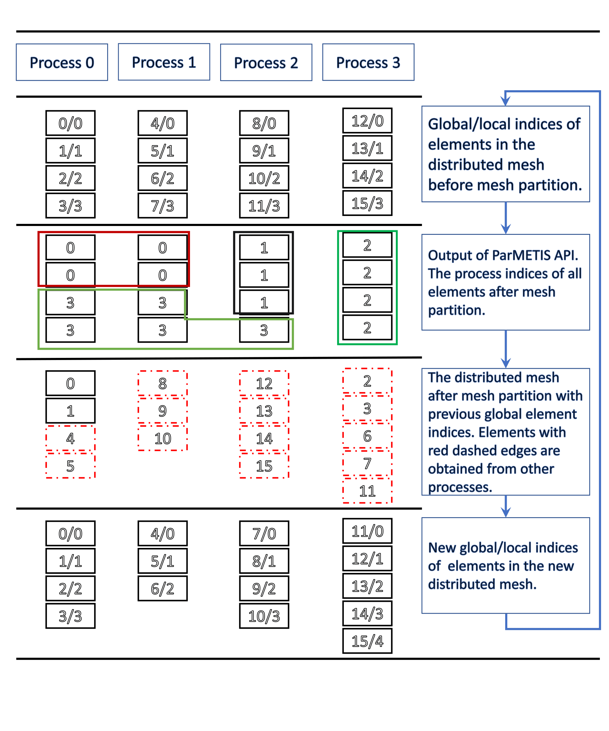
Figure 1: Illustration of the parallel mesh partitioning using the ParMETIS API.

For data redistribution, we use a collect-and-distribute strategy. We utilize MPI_Allgather() to gather all the conservative variables on all the processes and each process will fetch the corresponding working variables from the collected data pool. The aforementioned randomness of redistributing elements to all processes leads to the fact that when it comes to data redistribution, the elements on many of the processes could be totally different from those before the parallel mesh partitioning. This implies that the cost of a process-to-process communication strategy to exchange CFD data could possibly be close to that of the collect-and-distribute stategy. Besides, the coding complexity of the process-to-process strategy is overwhelming. In our numerical experiments, we have found that the total amount of run time needed for mesh partitioning and data redistribution is trivial when compared to that of implicit time-stepping. We would like to clarify that in the spatial and temporal solvers, communication among all processes is done in a process-to-process manner to maximize efficiency.

An important input of ParMetis_V3_AdaptiveRepart() is the weight of each element in the distributed mesh. For the FR discretization, the number of solution points $n_{sp}$ within a element is $(p+1)^{3}$ for a hexahedral element. And there are five equations at each solution point to be solved in three dimensional problems. Hence, the number of degrees of freedom in one element is $n_{dof}=5n_{sp}$. For a hexahedral element, all operations of the FR/CPR methods are indeed conducted dimension by dimension. Therefore, we roughly estimate the computational complexity of one-time residual evaluation as $O\left(n_{dof}\cdot(p+1)\right)$. When implicit time integrators are employed, the cost of one-time residual evaluation is trivial compared to three major parts, (a) evaluating the element Jacobian matrix,(b) calculating the element-Jacobi preconditioner and (c) solving the nonlinear/linear equations using Newton/Krylov methods. When evaluating the element Jacobian matrix, the finite difference approach is used. For each element, there will be $n_{dof}$ times the residual evaluation and the computational complexity is $O(n_{dof}^{2}\cdot(p+1))$. We use lower-upper (LU) decomposition to invert the element Jacobian matrix to obtain the element-Jacobi preconditioner. The computational complexity of is $O(n_{dof}^{3})$. In the matrix-free implementation of the GMRES solver, the approximation of matrix-vector product and preconditioning will contribute to the computational cost dominantly. For the matrix-vector product approximation, the computational cost will be that of one-time residual evaluation. The left preconditioning is used in our approach and the complexity is $O(n_{dof}^{2})$. Overall, the complexity of the Newton-Krylov solver is $G(O(n_{dof}^{2})+O\left(n_{dof}\cdot(p+1)\right)$, where $G$ is the total number of GMRES iterations in the pseudo transient continuation. $G$ is highly problem dependent. Thus, three candidates to calculate the weight of each element, namely, $\omega_{e}=n_{dof}/5=n_{sp}$, $\omega_{e}=n_{sp}^{2}$, and $\omega_{e}=n_{sp}^{3}$, can be investigated.

Though we can sketch the computational complexity within each element to pursue an optimal candidate for weight calculation, the parallel performance is only directly related to the output distributed mesh of ParMETIS. In our numerical experiments, we observe that when the disparity of element weights is excessively large, e.g., $w_{e}=n_{sp}^{3}$, $p_{min}=2$, and $p_{max}=5$, the output mesh will lead to degraded parallel efficiency and the large disparity will occasionally lead to failure of ParMETIS, even when $p$ is smaller than $4$ and $w_{e}=n_{sp}$ is used. Specifically, there will be processes which have no elements after parallel mesh partitioning. Therefore, when ParMETIS failure is encountered, we will decrease the weight of each element to $w_{e}=p+1$ and redo the mesh partitioning for the current time step. Note that the computational cost of parallel mesh partitioning is trivial compared to implicit time-stepping. In the following subsection, a simple example is employed to demonstrate the proposed dynamic load balancing strategy.

3.3 A simple example of dynamic load balancing

We simulate the 2D isentropic vortex propagation on a 3D mesh (obtained by extruding a 2D mesh in the $z$ direction for two layers) to demonstrate the dynamic load balancing strategy. The free stream condition is $(\rho,u,v,w,\text{Ma})^{\intercal}=(1,1,1,0,0.5)^{\intercal}$. The fluctuation is defined as [52]

$$\begin{cases}\delta u=-\frac{\alpha}{2\pi}(y-y_{0})e^{\phi(1-r^{2})},\\ \delta v=\frac{\alpha}{2\pi}(x-x_{0})e^{\phi(1-r^{2})},\\ \delta w=0,\\ \delta T=-\frac{\alpha^{2}(\gamma-1)}{16\phi\gamma\pi^{2}}e^{2\phi(1-r^{2})},\\ \end{cases}$$ (26)

where $\phi=\frac{1}{2}$ and $\alpha=5$ are parameters that define the vortex strength. $r=(x-x_{0})^{2}+(y-y_{0})^{2}$ is the distance from any point $(x,y,z)$ to the center of line the vortex $(x_{0},y_{0},z)=(0,0,z)$ at $t=0$. The domain is within $[-10,10]\times[-10,10]\times[0,0.8]$. A uniform mesh of $50\times 50\times 2$ elements is used for the numerical experiments. Periodic boundary conditions are imposed on all boundaries. We only simulate this problem for 60 steps with a time step size $\Delta t=0.05$. In the pseudo transient continuation, $\Delta\tau_{init}=0.05$ and $\Delta\tau_{max}=10$ are used for SER. For the adaptive solver, the flow field is initialized using uniform $p_{max}$ discretization.

72 processes are employed in this section. Herein, we take $p^{5}$ FR with $p$-adaptation as an example to show how the elements will be distributed to all processes. Elements in the first seven processes and the corresponding order-of-accuracy distribution, i.e., $(p+1)$ distribution, of four consecutive time steps are presented in Figure 2. From $t=0.15$ to $t=0.20$, the local polynomial degree at non-critical region will be coarsened to $p_{min}=1$ while a circular region surrounding the vortex will maintain high polynomial degrees. Due to this coarsening, the redistributed mesh change drastically. From $t=0.20$ to $t=0.25$, all the first seven process except the third one do not exchange any elements with other processes. From $t=0.25$ to $t=0.3$, even though the order-of-accuracy distribution only changes slightly, almost all the seven processes will send a large portion of local elements to other processes and obtain a significant amount of elements from other processes. For turbulence simulation, we anticipate that the change of the distributed mesh will be more dramatic than this simple problem.

In Figure 3, numerical results from $p/p_{max}$-refinement studies for the FR solver with/without adaptation are presented. From Figure 33(a), it is observed that both the $p$-uniform solver and $p$-adaptive solver have spectral convergence. The errors of the $p$-adaptive and $p$-uniform solvers are on the same magnitude when the highest polynomial degrees are the same. Run time of different solvers and the run time reduction of the $p$-adaptive solver using different weight algorithms (with respect to the $p$-uniform solver) are illustrated in Figure 33(b) and Figure 33(c), respectively. Overall, with proper weights assigned to all the elements, around 80% run time reduction can be achieved via $p$-adaptation when $p_{max}\geq 3$ (highest order of accuracy is no smaller than 4). For $\omega_{e}=n_{sp}$, when $p_{max}>3$, the parallel efficiency will keep decreasing as $p_{max}$ increases. This is due to the fact the computational cost of the Jacobian matrix and preconditioner evaluation will grow at much larger rates than that of the one-time residual evaluation. When $p_{max}=5$, $\omega_{e}=n_{sp}^{2}$ and $\omega_{e}=n_{sp}^{2}(p+1)$ have better performance than $\omega_{e}=n_{sp}$. However, it is shown that $\omega_{e}=n_{sp}^{3}$ generally degrades the efficiency than other candidates. Especially, when $\omega_{e}=n_{sp}^{3}$ and $p_{max}=5$, the $p$-adaptive solver fails to finish the simulation within the time that the $p$-uniform solver needs. In order to achieve optimal performance, both the weight calculation and the parallel mesh partitioning algorithm should be taken into account. In the following section, we use $w_{e}=n_{sp}$ for the $p$-adaptive solver when it is applied to under-resolved turbulence simulation since we only consider $p_{max}\leq 3$.

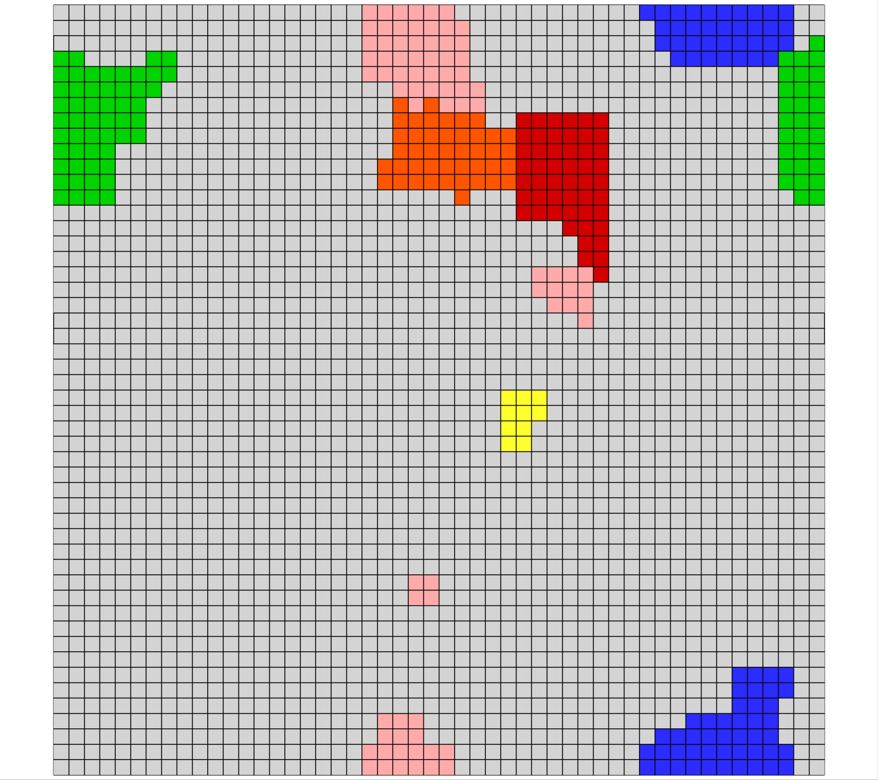
(a) $t=0.15$

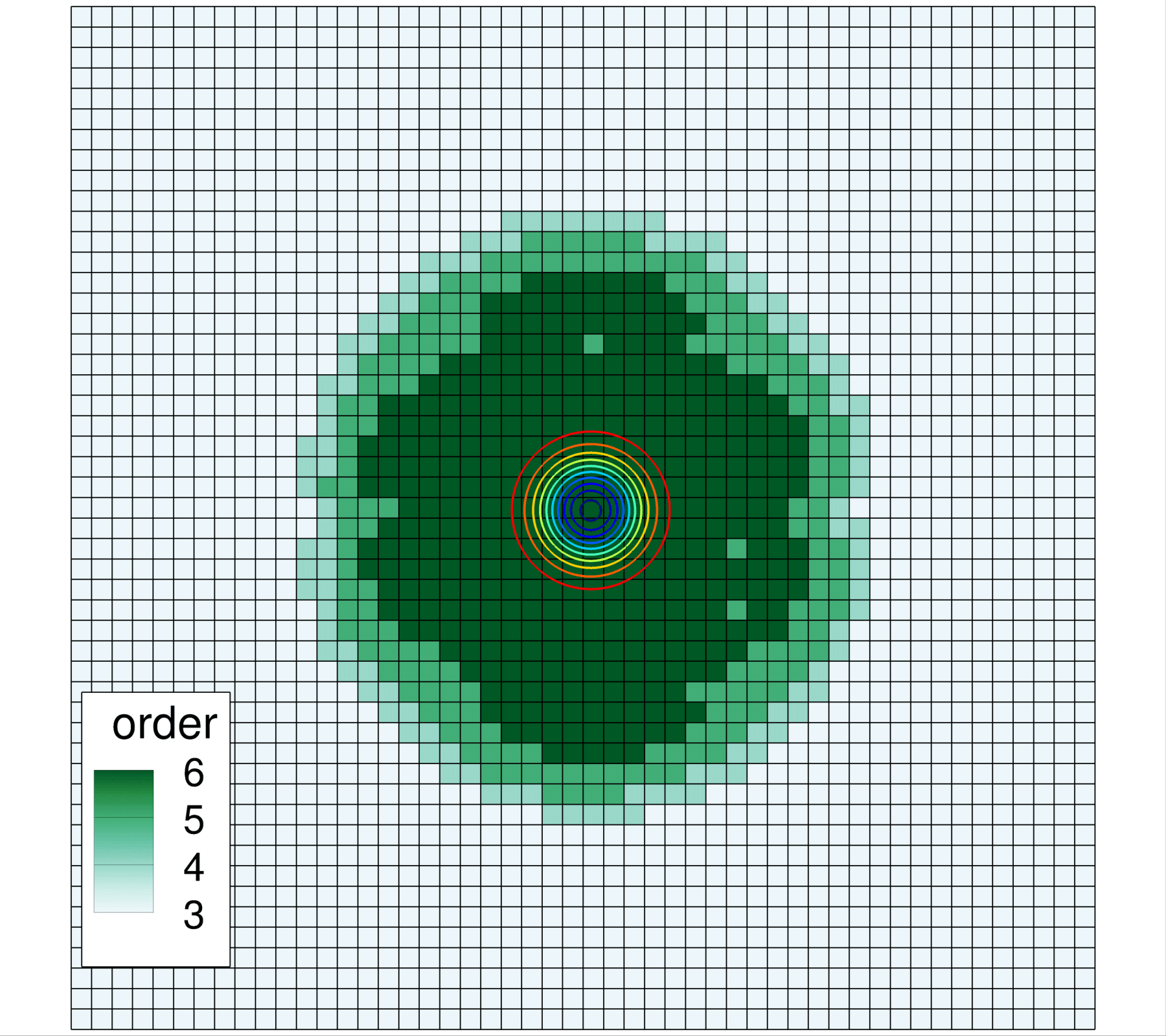
(b) $t=0.15$

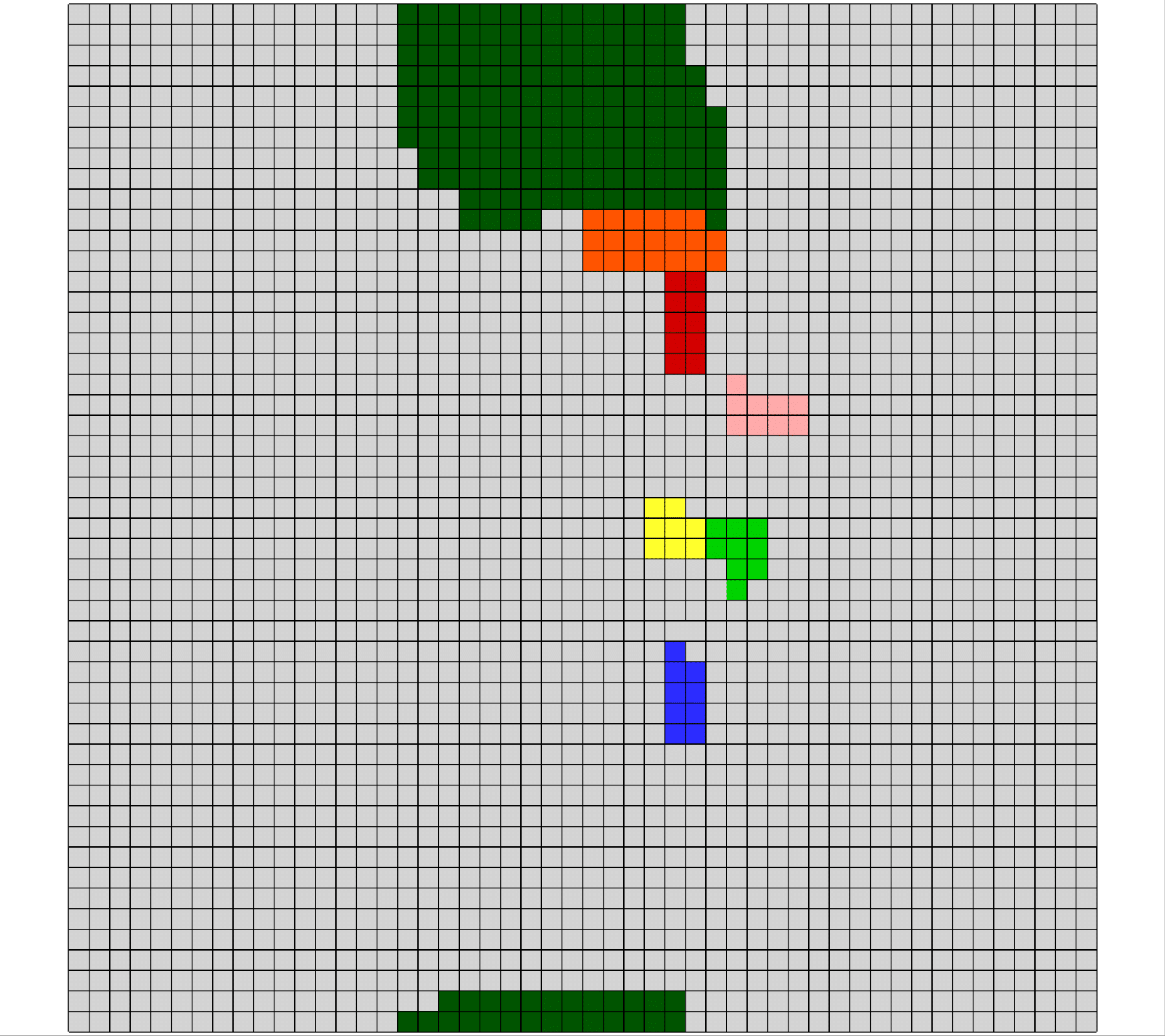
(c) $t=0.20$

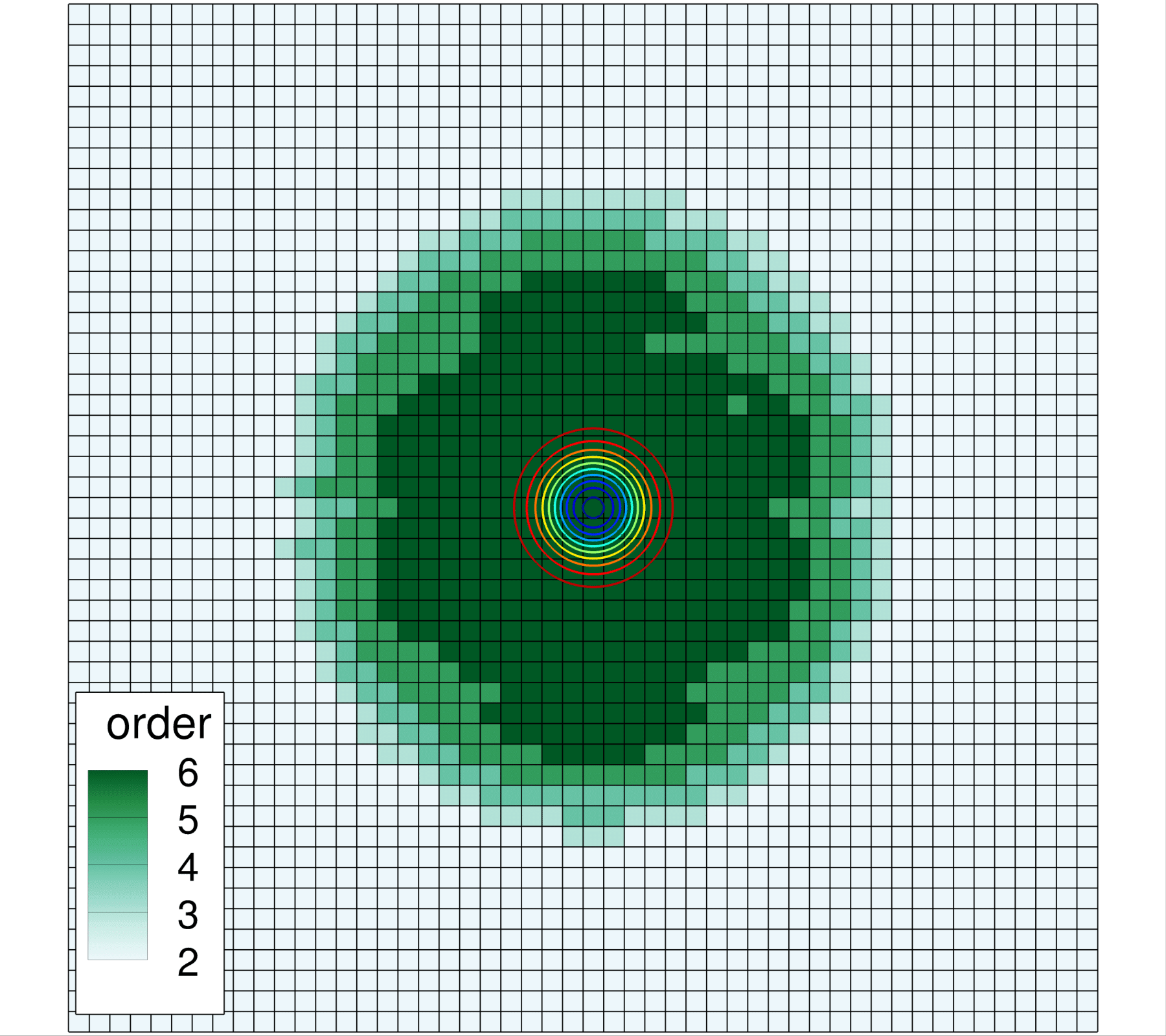
(d) $t=0.20$

(e) $t=0.25$

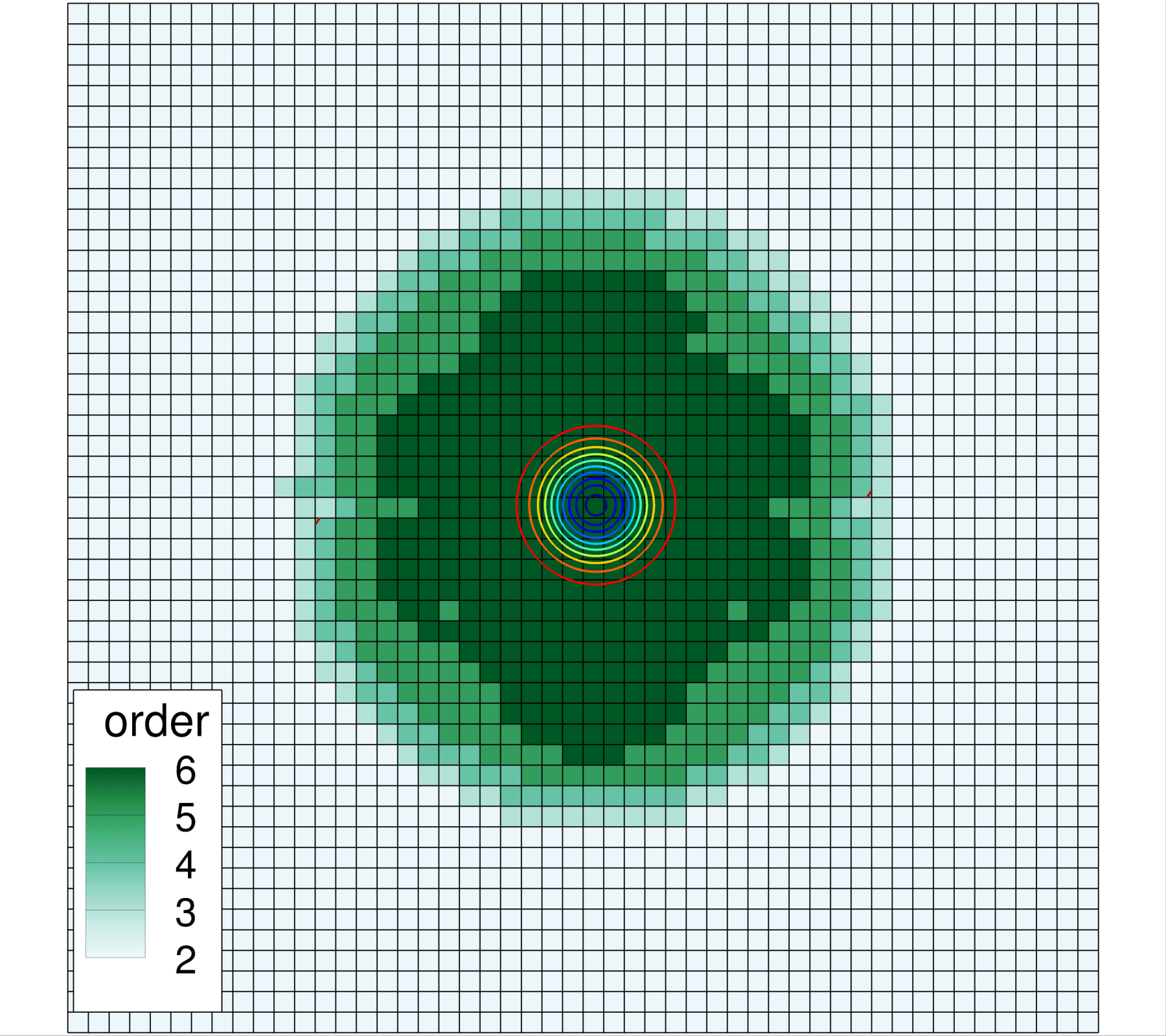
(f) $t=0.25$

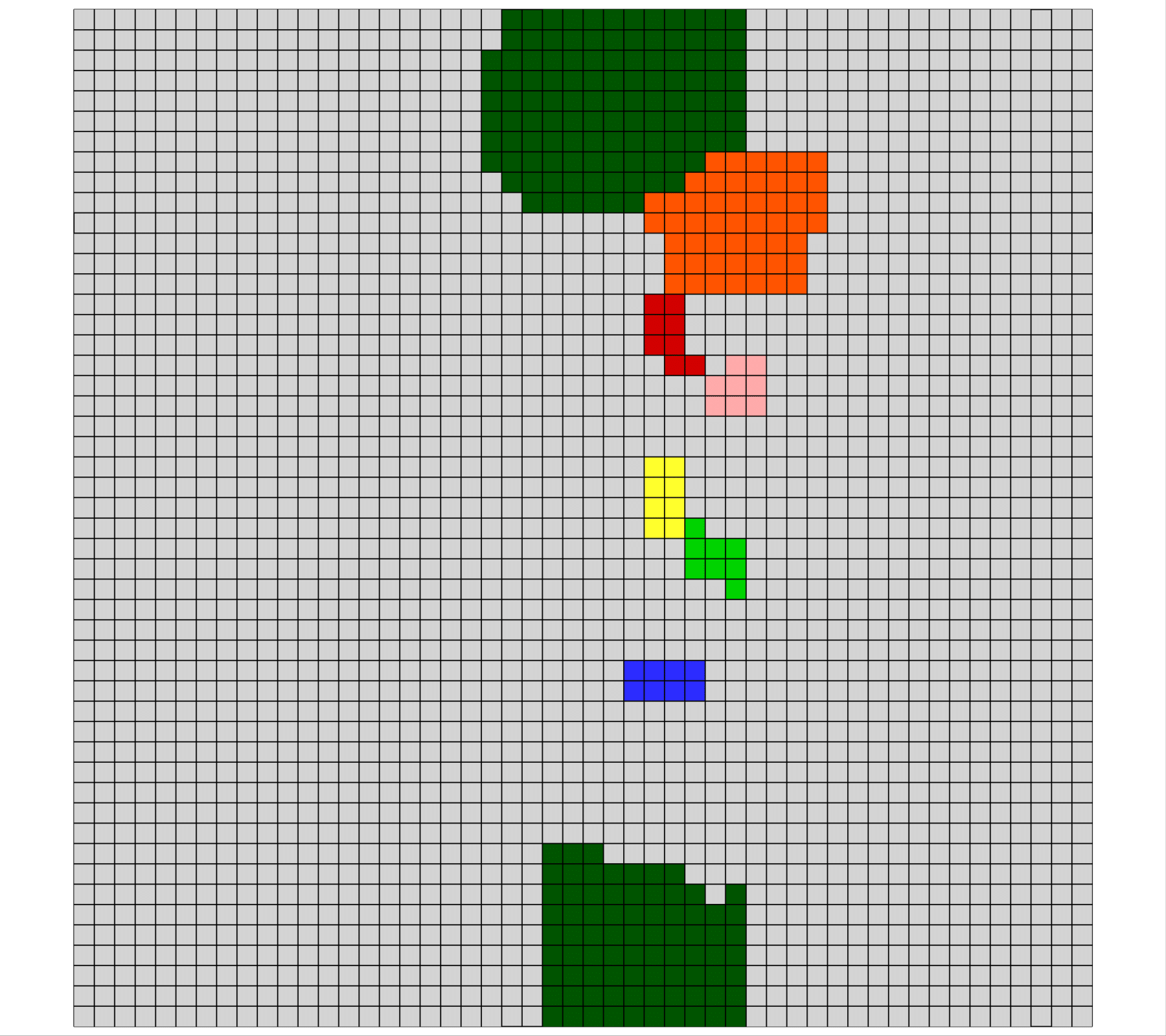
(g) $t=0.30$

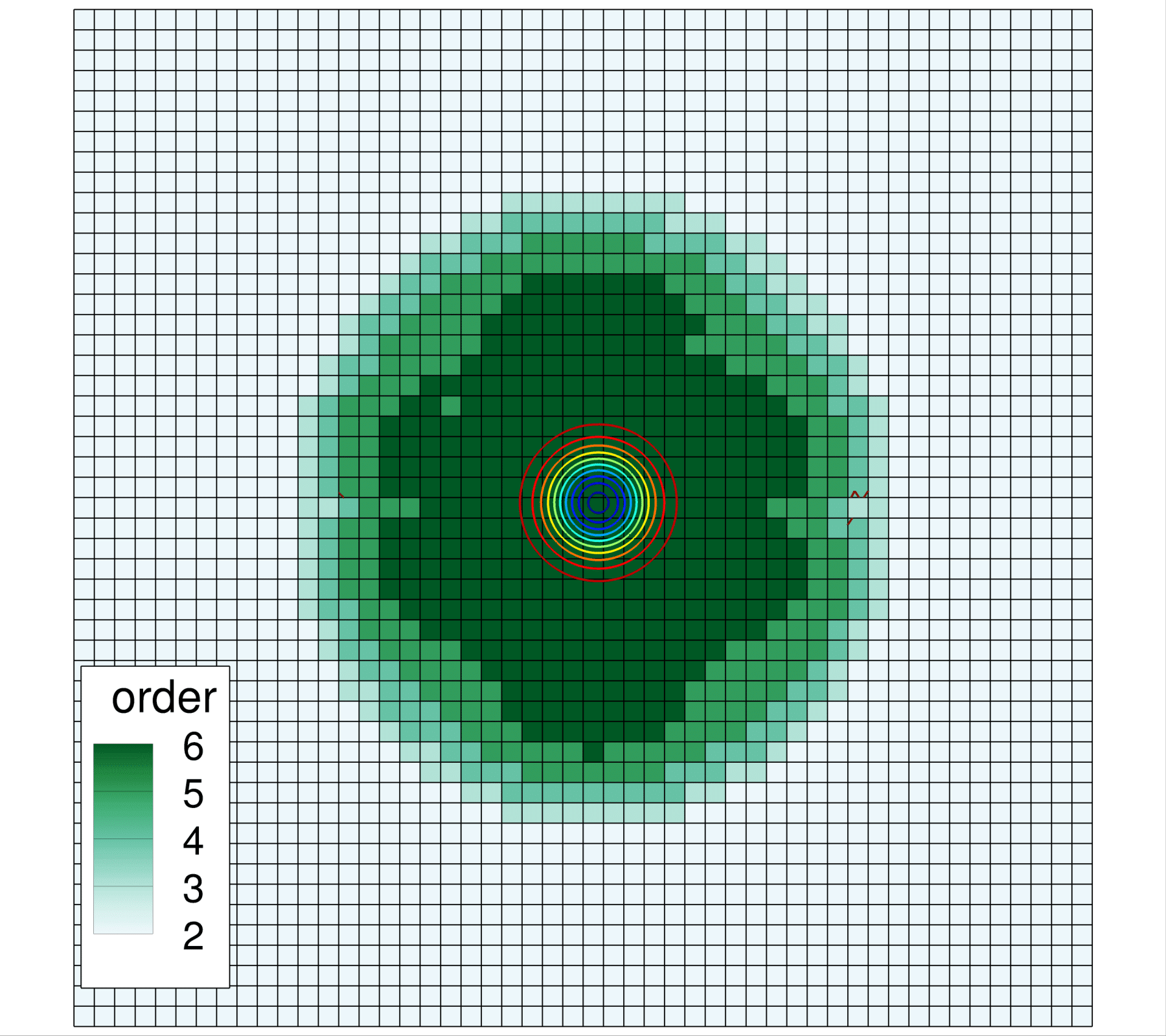
(h) $t=0.30$

Figure 2: (a), (c), (e), and (g) are elements in Processes 0–6 at four consecutive time steps. Processes 0–6 are colored by red, yellow, green, blue, orange, pink, and dark green, respectively. (b), (d), (f), and (h) are corresponding instantaneous order-of-accuracy distributions.

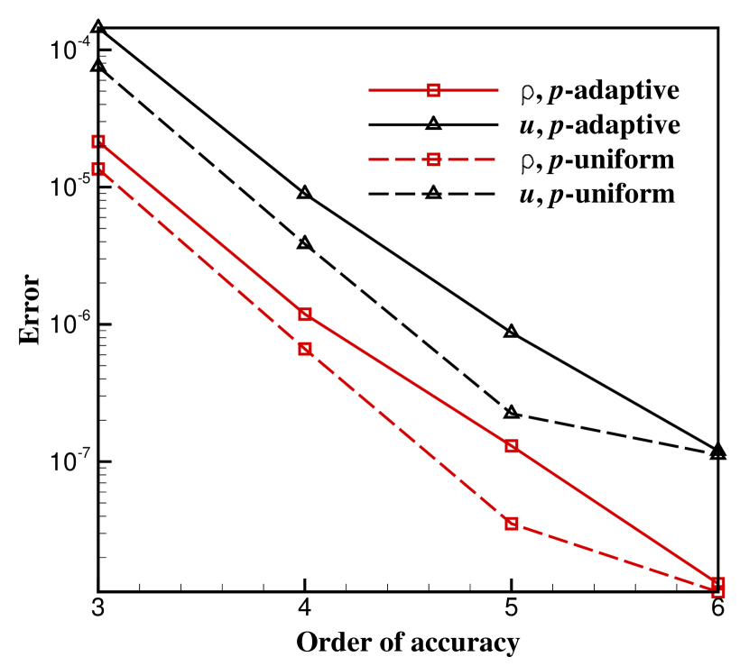
(a)

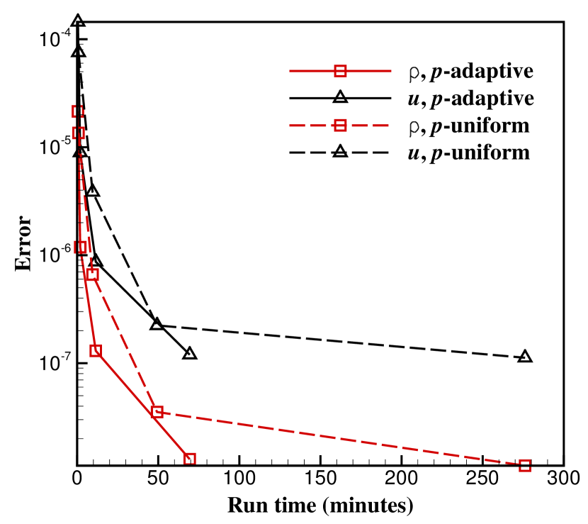
(b)

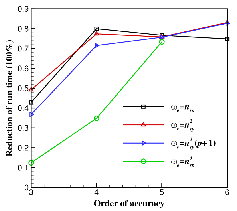
(c)

Figure 3: $p/p_{max}$-refinement of the $p$-uniform and $p$-adaptive FR solvers for the isentropic vortex propagation. (a) Error vs. order of accuracy, (b) error vs. run time, and (c) reduction of run time vs. order of accuracy. For the $p$-adaptive solver, the order of accuracy indicates the highest order of accuracy, i.e., $p_{max}+1$ in the flow field.

4 Applications to under-resolved turbulence simulation

The numerical studies in this section use seven computational nodes in a distributed-memory cluster. Each node has two 18-core Intel Xeon Gold 6140 Skylake CPUs (2.3 GHz clock speed, 24.75 MB L3 cache) and 384 GB memory ($12\times 32$ GB DDR4). The nodes are connected by a network of four 36-port EDR (Enhanced Data Rate) InfiniBand switches (100 Gb/s bandwidth, 90 ns latency). 252 processes are used for every simulation. The CFD codes and third party libraries, such as ParMETIS and PETSc, are compiled using MPICH 3.2.1 and GCC 7.3.0 compilers. The C++11 standard is used in the compilation of the CFD codes.

4.1 Under-resolved simulation of the flow over an infinite cylinder

Long time simulations of the transitional flow over an infinite cylinder are conducted to validate the reliability of the $p$-adaptive solver in this section. The diameter of the cylinder is $d=1$. The inflow conditions are set as the vector $(\rho_{\infty},u_{\infty},v_{\infty},w_{\infty},\text{Ma}_{\infty})^{\intercal}=(1,1,0,0,0.1)^{\intercal}$. The Reynolds number of the inflow with respect to the diameter of the cylinder is $\text{Re}_{d}={\rho_{\infty}u_{\infty}d}/{\mu}=3900$. The Prandtl number is $\text{Pr}=0.71$. A 2D view of the mesh is illustrated in Figure 4. The center of the cylinder sits at the origin. The 3D mesh is obtained by extruding the 2D mesh along the $z$ direction, i.e., $(0,0,1)^{\intercal}$, for eight layers and the thickness of each layer is $0.25d$. There are 17694 hexahedral elements and the curved wall boundary is represented by $p^{3}$ elements. $p^{2}$ and $p^{3}$ FR are employed with/without $p$-adaptation. The cylinder surface is treated as a no-slip adiabatic wall. Farfield boundary conditions are applied to outer boundaries. Periodic boundary conditions are imposed at the front and back sides. We employ ESDIRK4 for time integration and $\Delta t=0.025$. In the pseudo transient continuation, $\Delta\tau_{init}=0.001$ and $\Delta\tau_{max}=0.01$ are used for SER. The tolerance for the pseudo transient continuation is $tol_{rel}^{pseudo}=10^{-4}$ and that of the GMRES solver is $tol_{rel}^{gmres}=10^{-1}$. We run all simulations until $t_{end}=800$. The instantaneous solutions in $t\in(100,800]$ are used for time averaging. For $p^{2}$ FR with adaptation, $(\nu_{max},\nu_{min})=(0.1,0.001)$ and $(\nu_{max},\nu_{min})=(0.1,0.01)$ are tested. For $p^{3}$ FR, only $(\nu_{max},\nu_{min})=(0.1,0.01)$ is used to carry out the $p$-adaptation. The flow field is initialized uniformly with the inflow conditions and the $p$-adaptive solver starts from a uniform $p^{1}$ discretization.

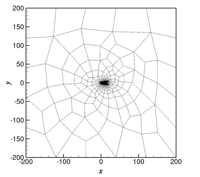
(a) Global view

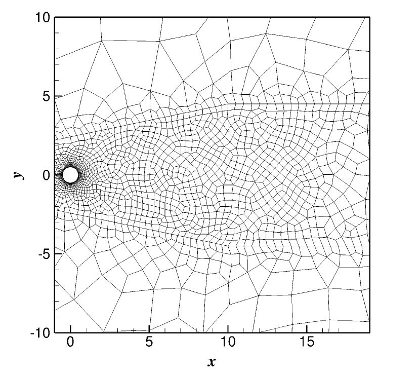
(b) Close-up view

Figure 4: 2D views of the unstructured mesh around a circular cylinder.

Table 1: Run time of all simulations of the transitional flow over the infinite cylinder.

Method	$(\nu_{max},\nu_{min})$	Run time	Reduction of	Reduction of
		(hours)	run time	$n_{sp}^{tot}$
$p^{2}$ FR	no adaptation	27.43	0	0
	$(0.1,0.001)$	22.43	18.23%	49.96% at $t=800$
	$(0.1,0.01)$	16.55	39.66%	63.43% at $t=800$
$p^{3}$ FR	no adaptation	149.78	0	0
	$(0.1,0.01)$	45.56	69.58%	75.98% at $t=800$

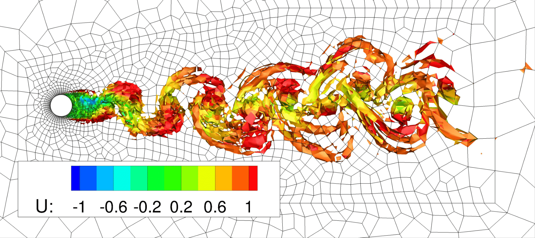
(a) $p^{2}$ FR without adaptation

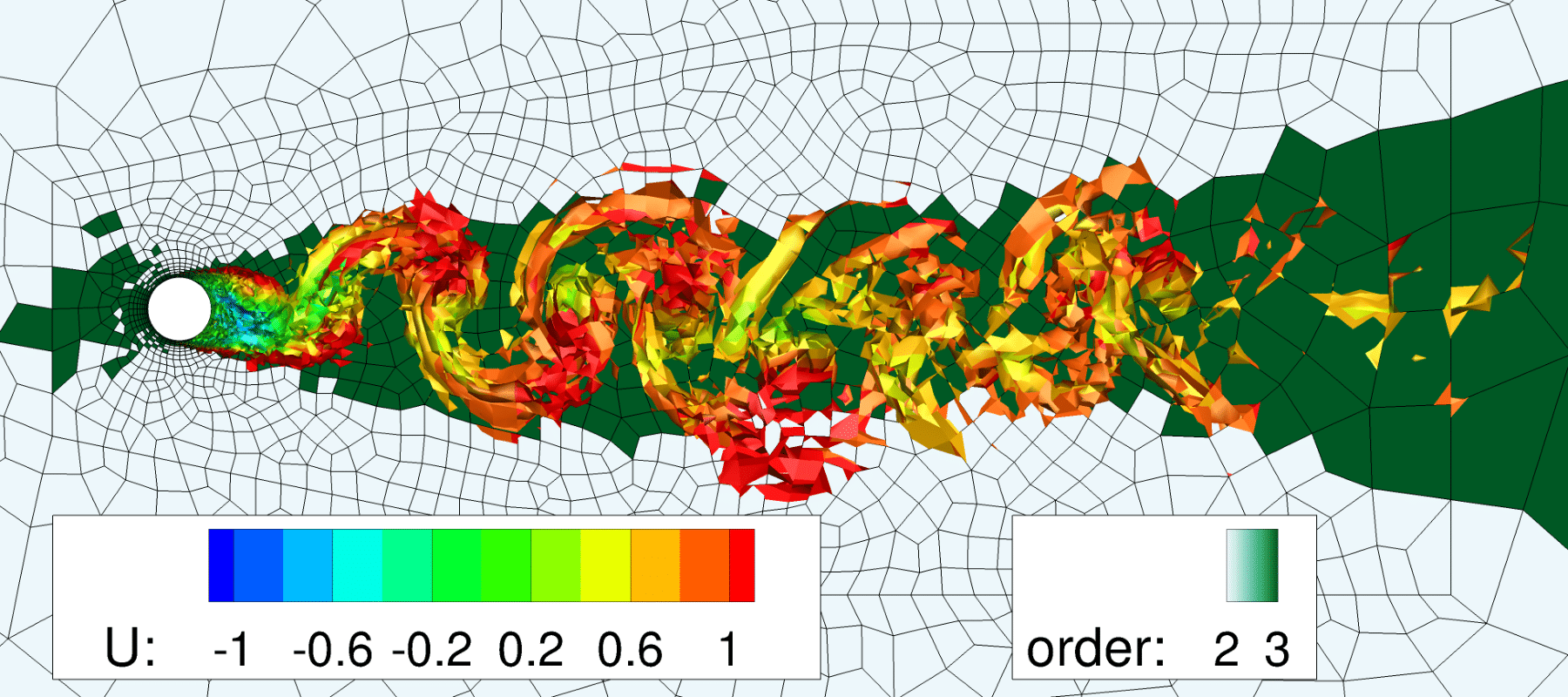
(b) $p^{2}$ FR with adaptation and $(\nu_{max},\nu_{min})=(0.1,0.001)$

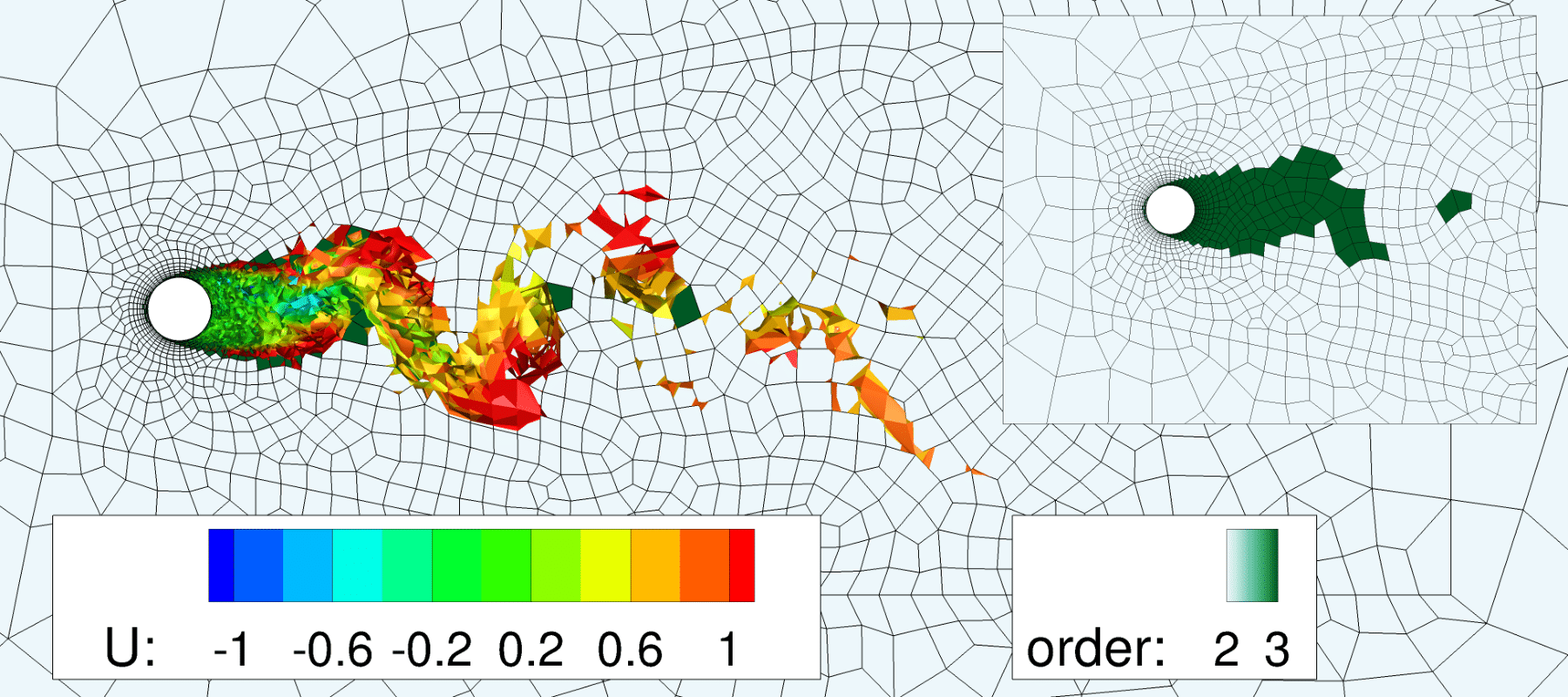
(c) $p^{2}$ FR with adaptation and $(\nu_{max},\nu_{min})=(0.1,0.01)$

Figure 5: Transitional flow over the infinite cylinder at $\text{Re}=3900$. Instantaneous isosurfaces of $Q=0.5$ colored by velocity component in the $x$ direction at $t=800$. Order-of-accuracy distribution at slice $z=0$ is turned on in (b) and (c). A close-up view of the near wall region is also presented in (c).

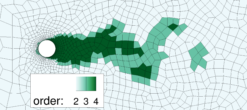
(a) $z=0.5$

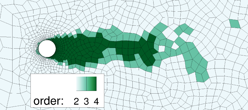
(b) $z=1$

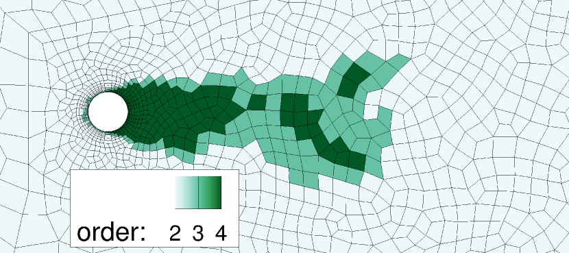
(c) $z=1.5$

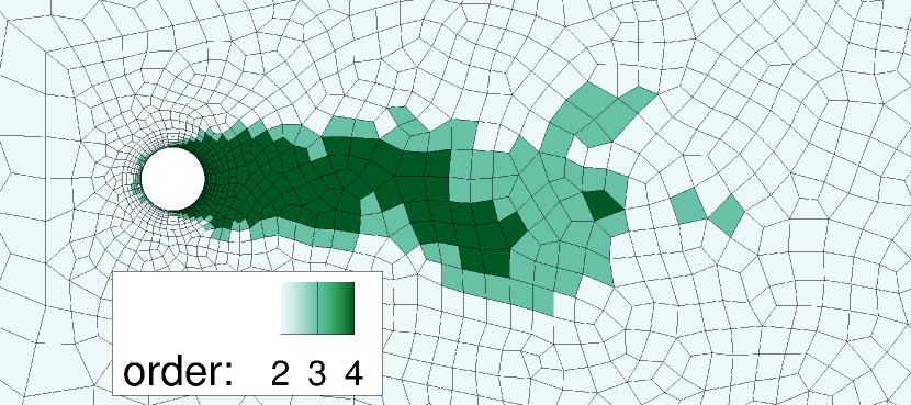
(d) $z=2$

Figure 6: Instantaneous order-of-accuracy distribution of $p^{3}$ FR with adaptation at different slices when $t=800$.

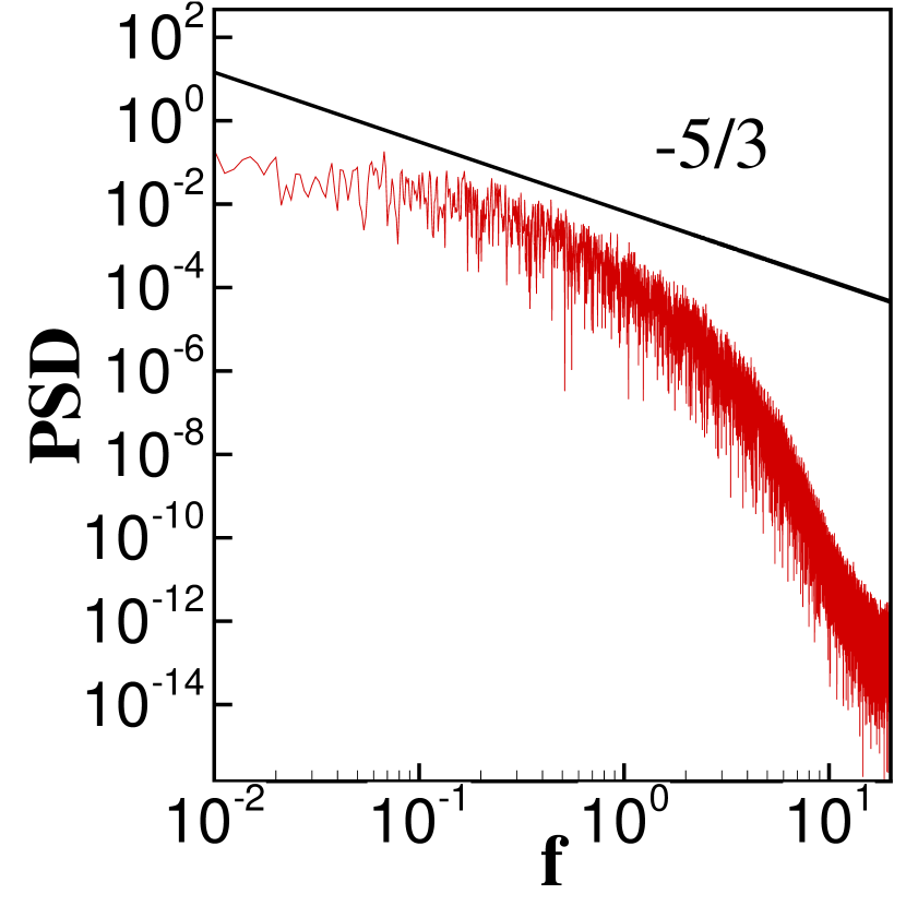
(a) $(0.58,0,1)^{\intercal}$

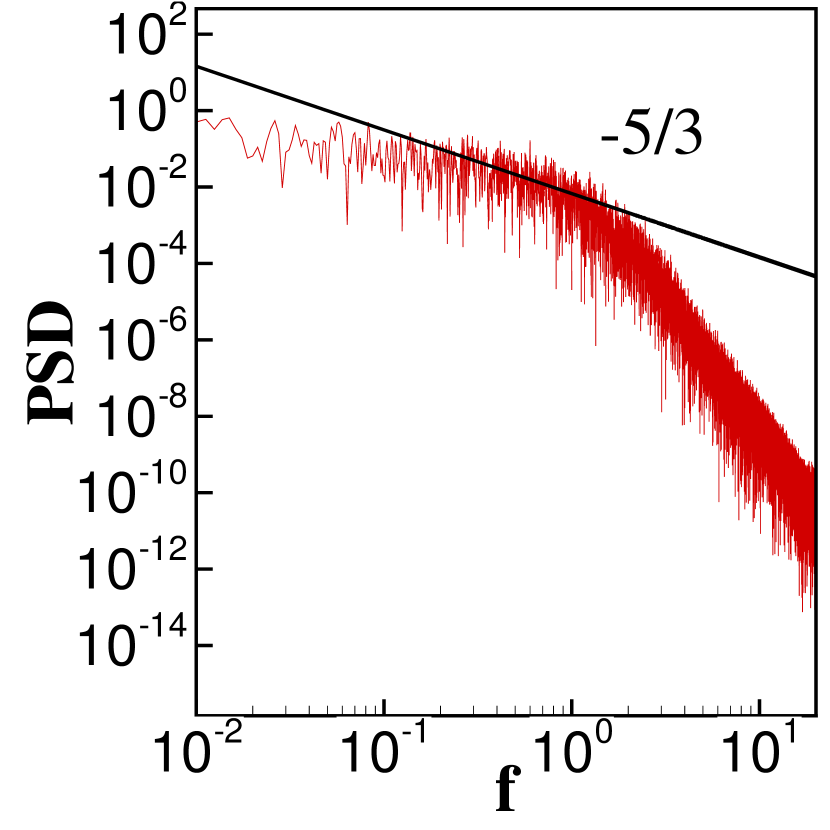
(b) $(1.54,0,1)^{\intercal}$

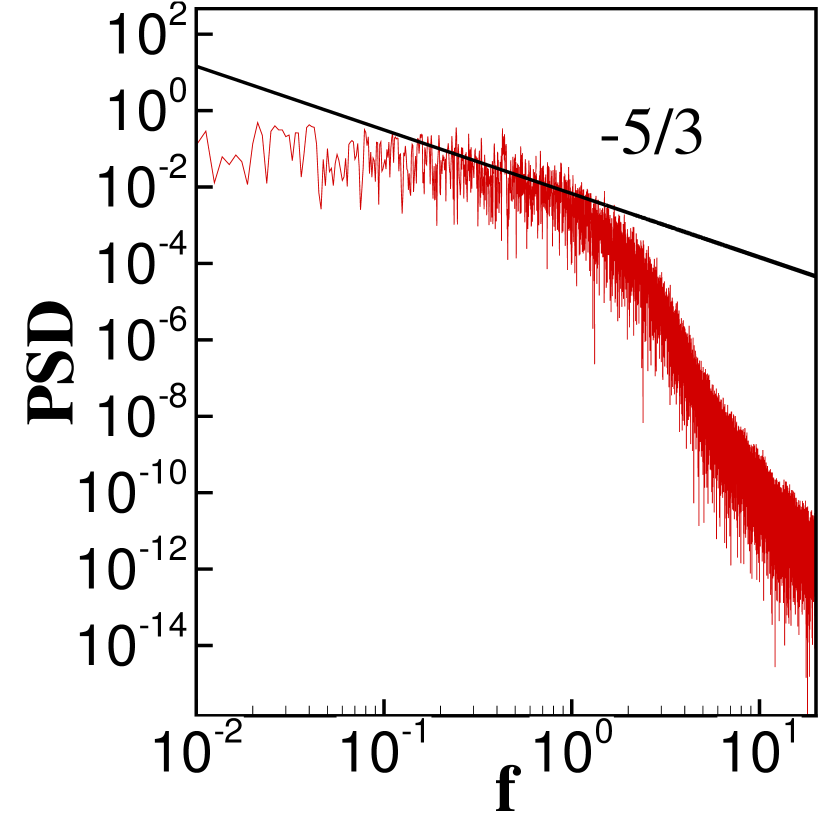
(c) $(6,0,1)^{\intercal}$

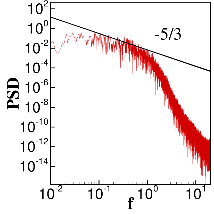
(d) $(10,0,1)^{\intercal}$

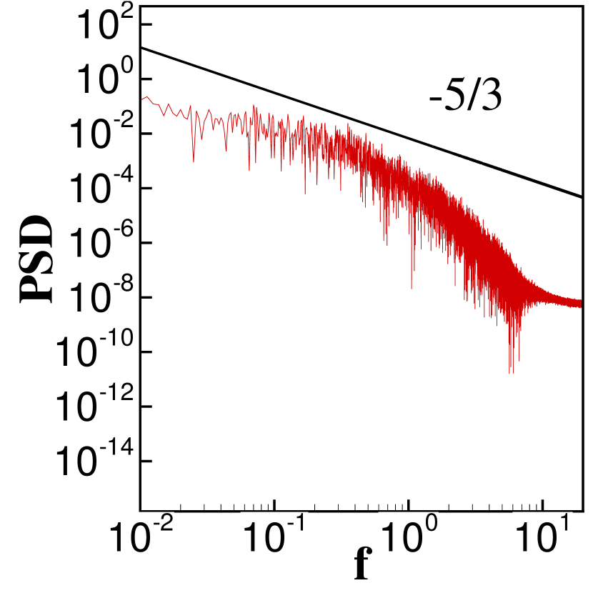
(e) $(0.58,0,1)^{\intercal}$

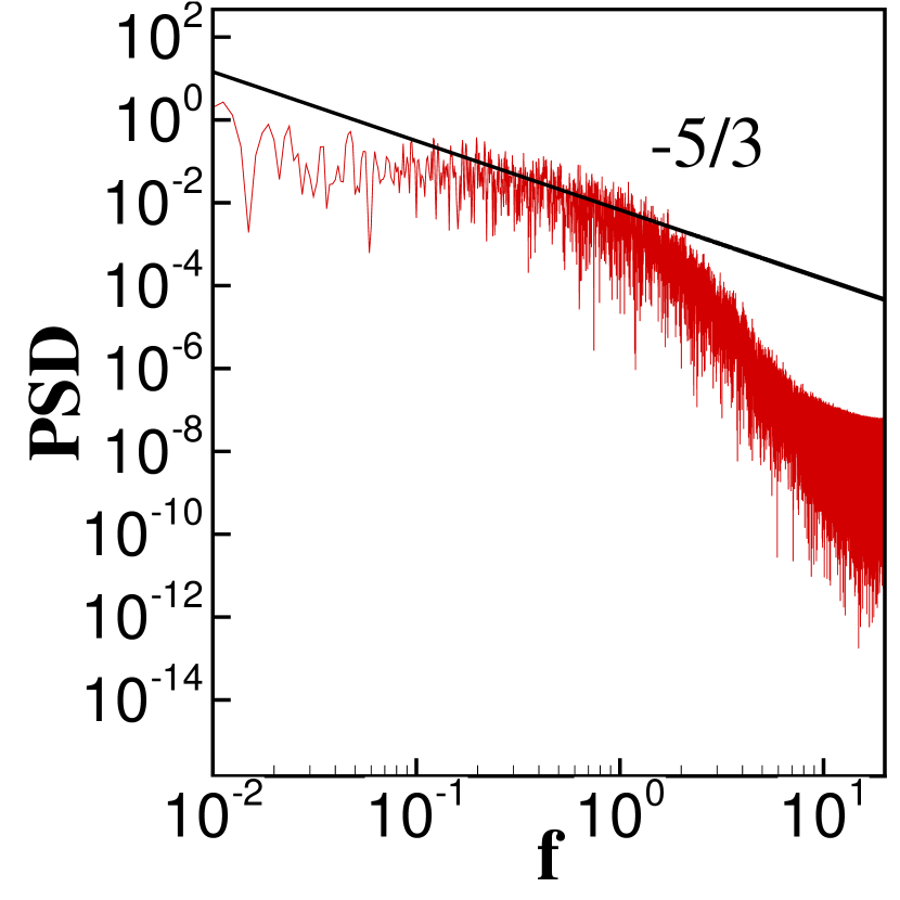
(f) $(1.54,0,1)^{\intercal}$

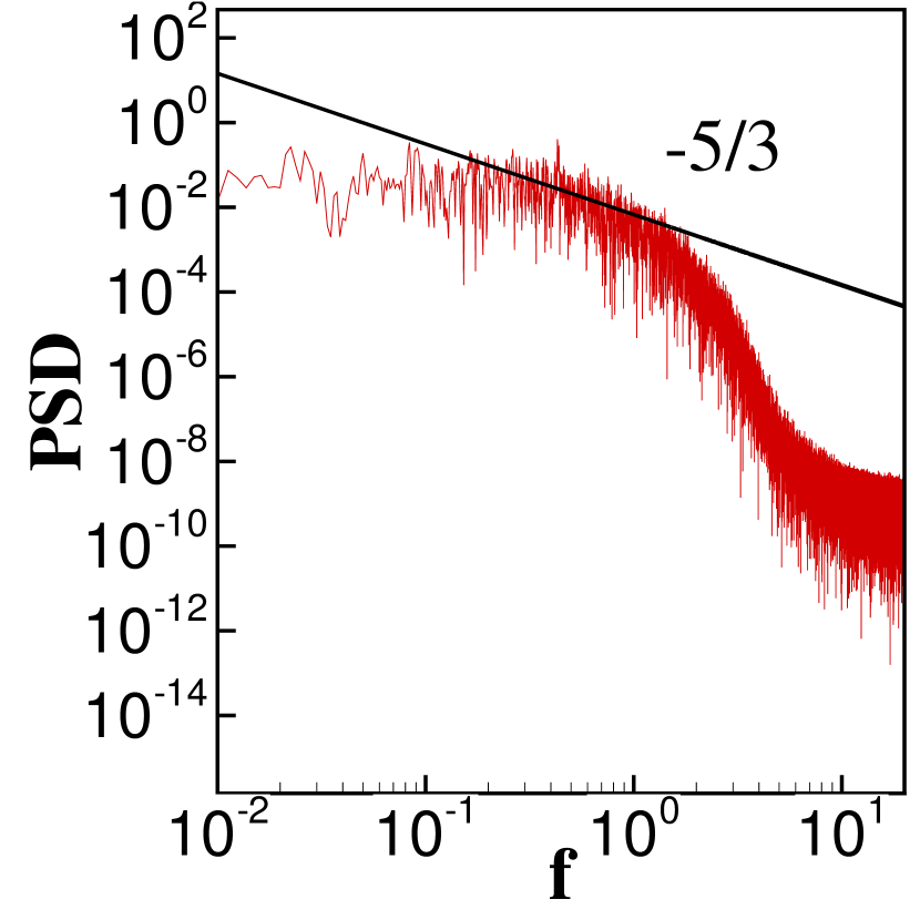
(g) $(6,0,1)^{\intercal}$

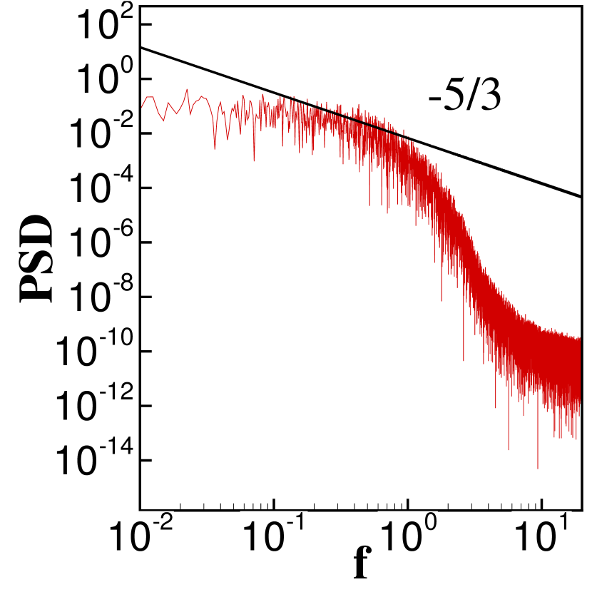
(h) $(10,0,1)^{\intercal}$

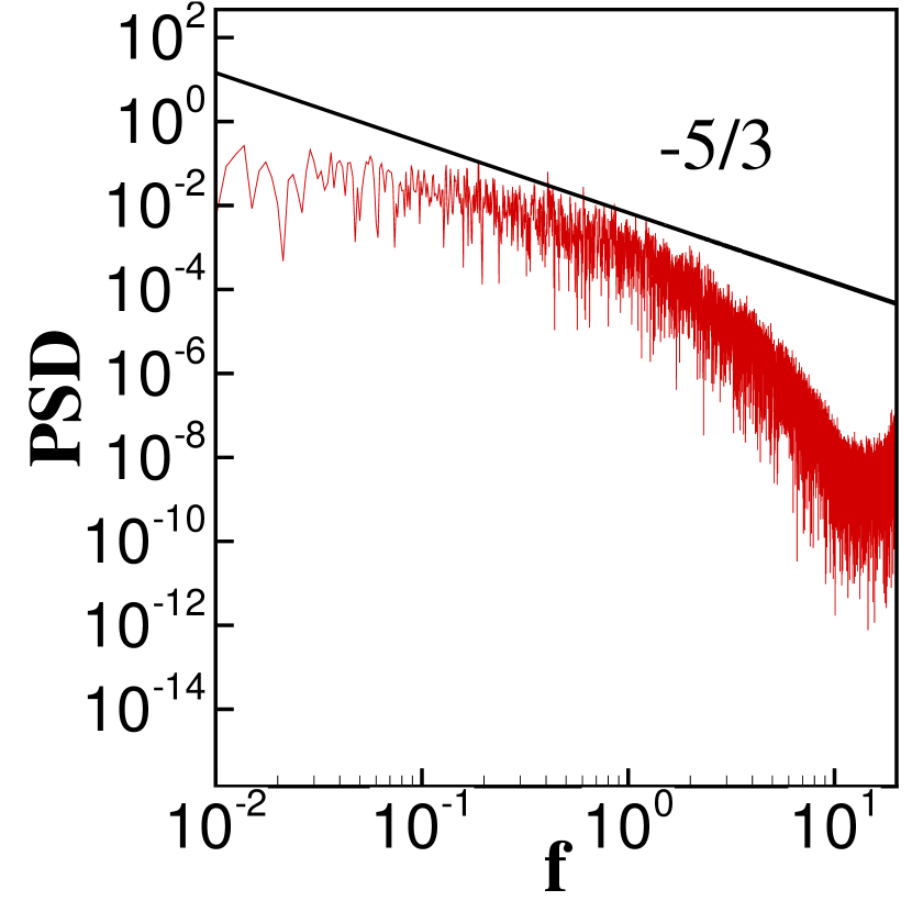
(i) $(0.58,0,1)^{\intercal}$

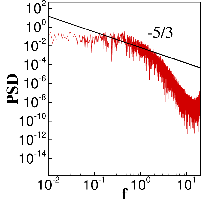
(j) $(1.54,0,1)^{\intercal}$

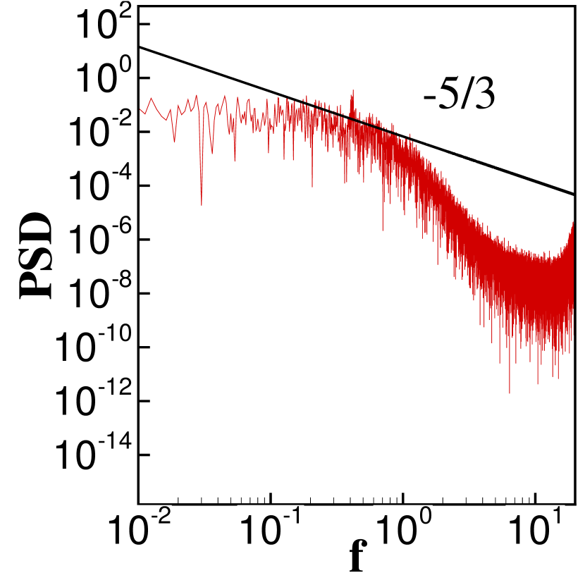
(k) $(6,0,1)^{\intercal}$

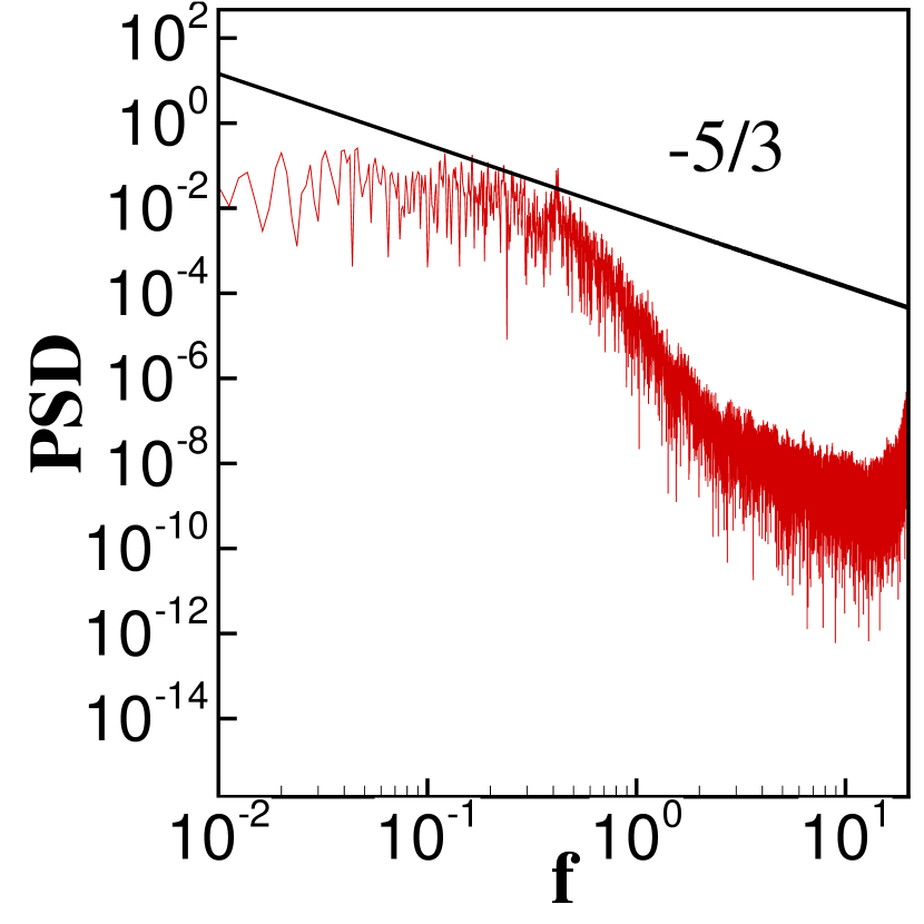
(l) $(10,0,1)^{\intercal}$

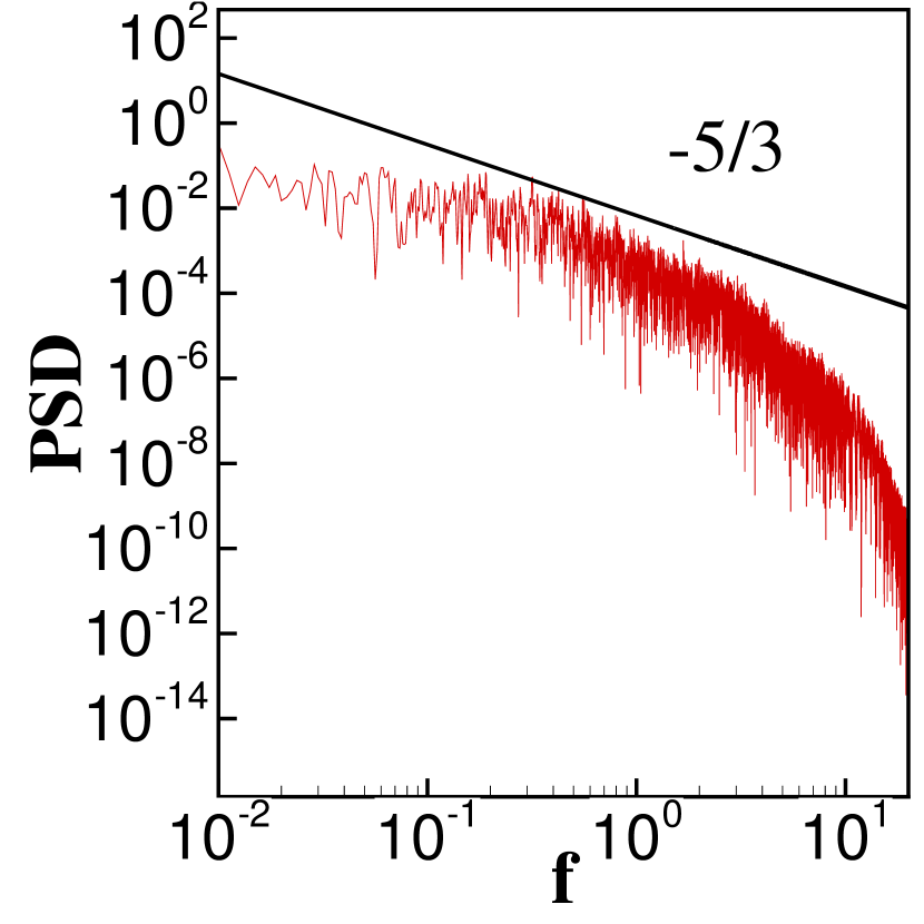
(m) $(0.58,0,1)^{\intercal}$

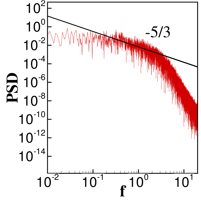
(n) $(1.54,0,1)^{\intercal}$

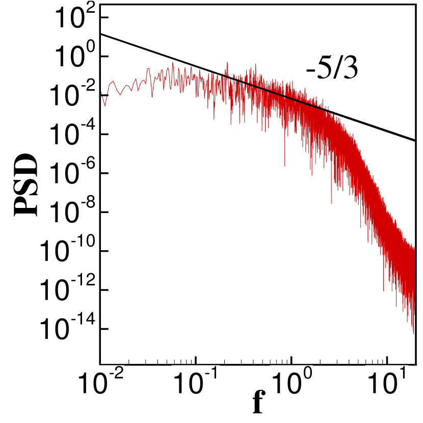
(o) $(6,0,1)^{\intercal}$

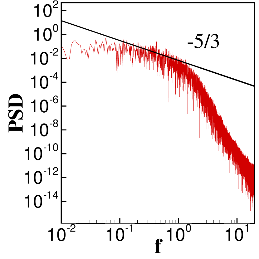
(p) $(10,0,1)^{\intercal}$

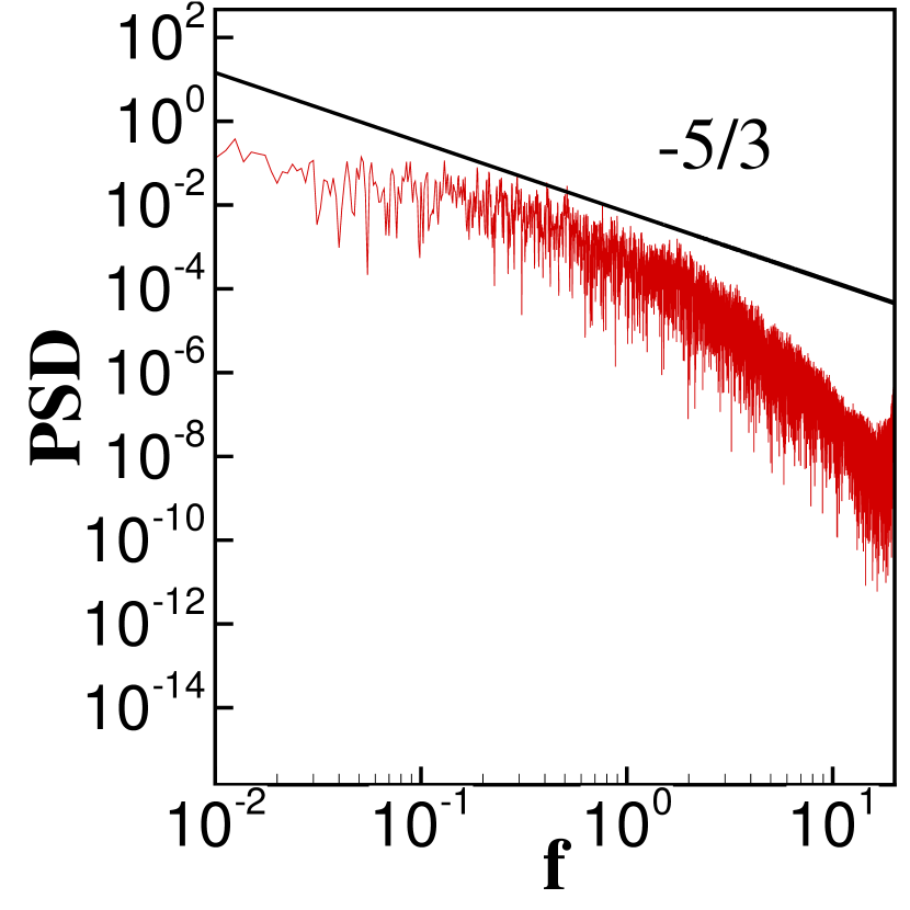
(q) $(0.58,0,1)^{\intercal}$

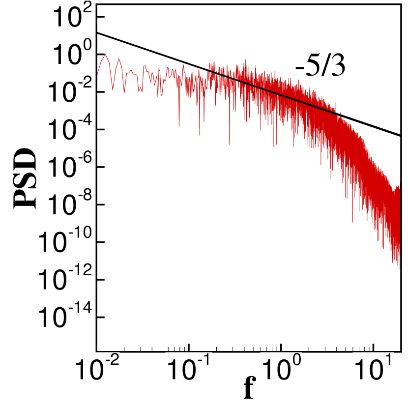
(r) $(1.54,0,1)^{\intercal}$

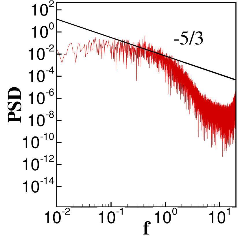
(s) $(6,0,1)^{\intercal}$

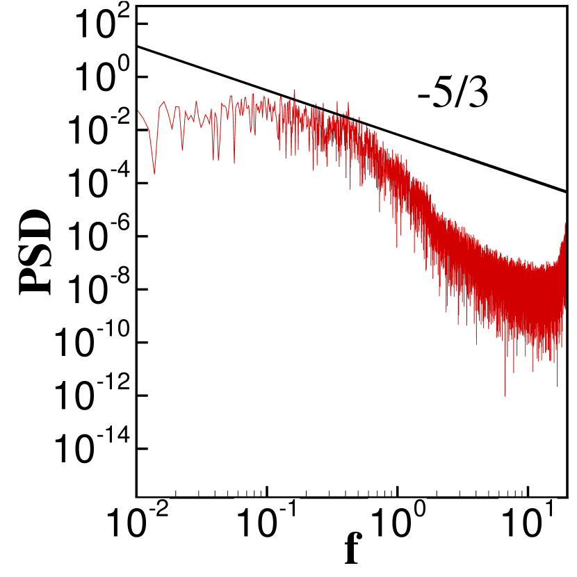
(t) $(10,0,1)^{\intercal}$

Figure 7: Power spectral density of the total velocity at different locations in the wake region. (a)–(d) adaptive $p^{2}$ FR without adaptation, (e)–(h) adaptive $p^{2}$ FR with $(\nu_{max},\nu_{min})=(0.1,0.001)$, (i)–(l) adaptive $p^{2}$ FR with $(\nu_{max},\nu_{min})=(0.1,0.01)$, (m)–(p) $p^{3}$ FR without adaptation, and (q)–(t) adaptive $p^{3}$ FR with $(\nu_{max},\nu_{min})=(0.1,0.01)$. A line of slope $-5/3$ is added to every graph as a reference.

The run time of all simulations is documented in Table 1. Overall, the $p$-adaptive solver can reduce a significant amount of run time. Particularly, for $p^{3}$ FR, the adaptive solver can reduce the run time by 69.58% when $(\nu_{max},\nu_{min})=(0.1,0.01)$. At $t=t_{end}$, the adaptive $p^{2}$ FR solver has 239,073 solution points when $(\nu_{max},\nu_{min})=(0.1,0.001)$ and 17,4701 solution points when $(\nu_{max},\nu_{min})=(0.1,0.01)$; the adaptive $p^{3}$ FR solver has 271,958 solution points. When the turbulence is fully developed, the total number of $p$-refined elements will be similar at different time steps. In general, the reduction of run time and that of $n_{sp}^{tot}$ are consistent with each other and $p$-adaptation with larger $p_{max}$ is encouraged as shown in Table 1. From the isosurfaces of $Q$-criterion, where $Q=0.5$, illustrated in Figure 5, it is intuitive that the $p$-adaptive solver is more dissipative than $p$-uniform solver in the wake region away from the cylinder. The order-of-accuracy distributions of the adaptive solver with different adaptation parameters at slice $z=0$ are also presented. When $\nu_{min}$ is decreased from $0.01$ to $0.001$, the $p^{2}$ region will substantially extend into the wake region away from the cylinder. Thus, the reduction in run time will decrease. The order-of-accuracy distributions of the adaptive $p^{3}$ FR solver at different slices are shown in Figure 6 to give a better presentation of the local $p$-adaptation.

We further examine the power spectral density (PSD) of the total velocity at four locations in the wake region, namely $(0.58,0,1)^{\intercal}$, $(1.54,0,1)^{\intercal}$, $(6,0,1)^{\intercal}$, and $(10,0,1)^{\intercal}$ as presented in Figure 7. A reference line of slope $-5/3$ is included in every graph. Compared to the DNS results in [66], a large portion of the inertial range can be resolved at the first two points. At the last two points, $(6,0,1)^{\intercal}$, and $(10,0,1)^{\intercal}$, the adaptive solver gets more dissipative as the parameter $\nu_{min}$ increases. The velocity profiles at different positions on the $x$-axis in Figure 8, where $y/d\in[-3,3]$, further demonstrates this observation. At $x=0.58$ and $x=1.54$, the velocity profiles of the $p$-adaptive FR methods are close to those of the $p$-uniform FR methods. At $x=6$ and $x=10$, the local extrema of the $p$-adaptive FR are largely dissipated, even when $(\nu_{min},\nu_{max})=(0.1,0.001)$.

The surface pressure coefficient $C_{p}$ and surface friction coefficient $C_{f}$ on the $y>0$ side of the cylinder are presented in Figure 9. When $(\nu_{max},\nu_{min})=(0.1,0.001)$, the results of the adaptive $p^{2}$ FR method is close to that of the $p$-uniform $p^{2}$ FR method. When $(\nu_{max},\nu_{min})=(0.1,0.01)$, the results of adaptive solver are still comparable to those of the $p$-uniform solver even though a large portion of the wake region uses $p^{1}$ polynomials only.

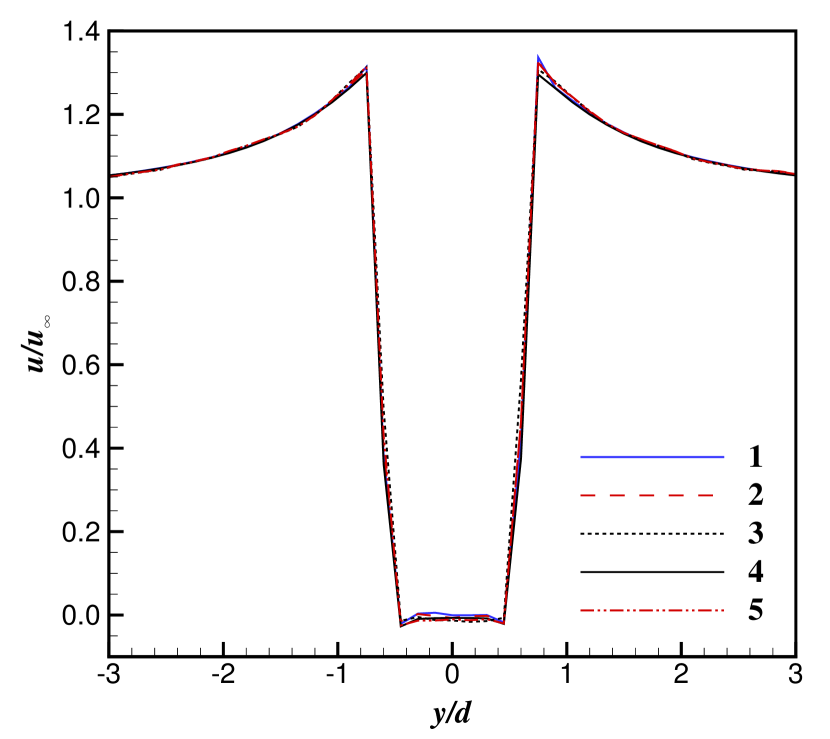
(a) $x=0.58$

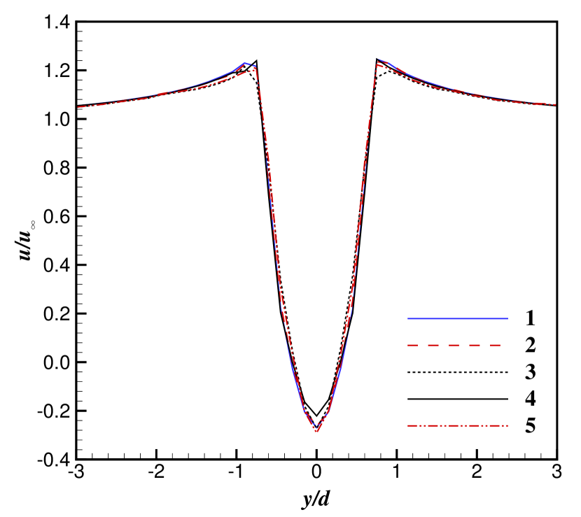
(b) $x=1.54$

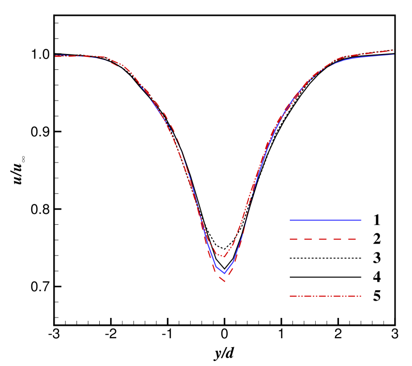
(c) $x=6$

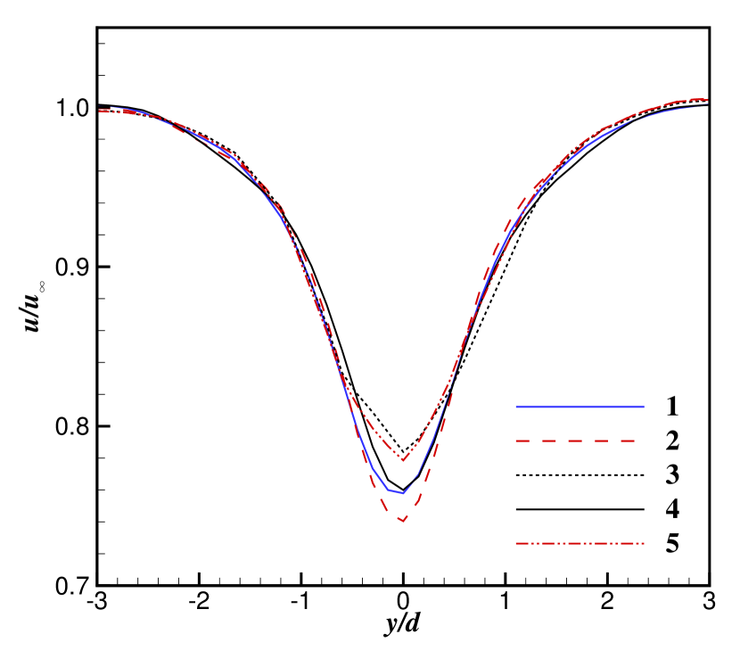
(d) $x=10$

Figure 8: Profiles of velocity component $u$ in $x$-direction at different locations. Legend 1, $p$-uniform $p^{2}$ FR; Legend 2, $p$-adaptive $p^{2}$ FR with $(\nu_{max},\nu_{min})=(0.1,0.001)$; Legend 3, $p$-adaptive $p^{2}$ FR with $(\nu_{max},\nu_{min})=(0.1,0.01)$; Legend 4, $p$-uniform $p^{3}$ FR; Legend 5, $p$-adaptive $p^{3}$ FR with $(\nu_{max},\nu_{min})=(0.1,0.01)$;

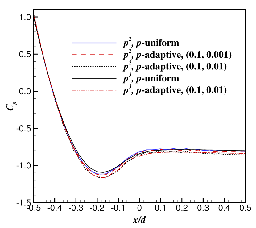
(a) Surface pressure coefficient $C_{p}$

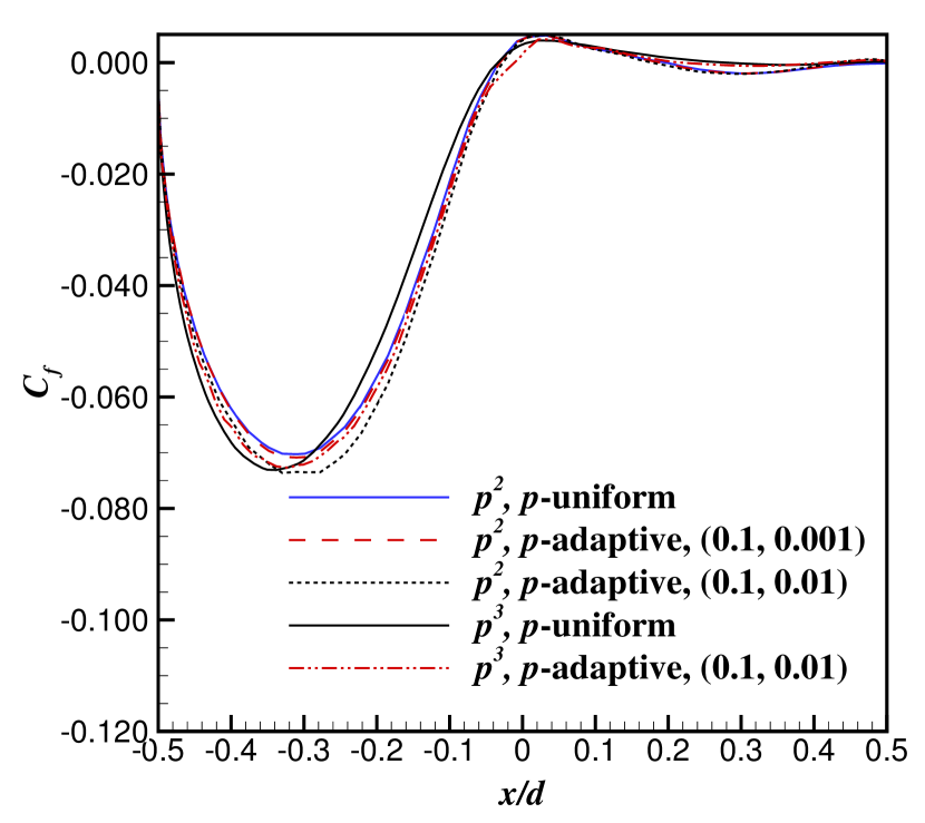
(b) Surface friction coefficient $C_{f}$

Figure 9: Surface $C_{p}$ and $C_{f}$ in the averaged field of the transitional flow over the infinite cylinder at $\text{Re}=3900$.

4.2 Under-resolved simulation of the transitional flow over the SD7003 wing

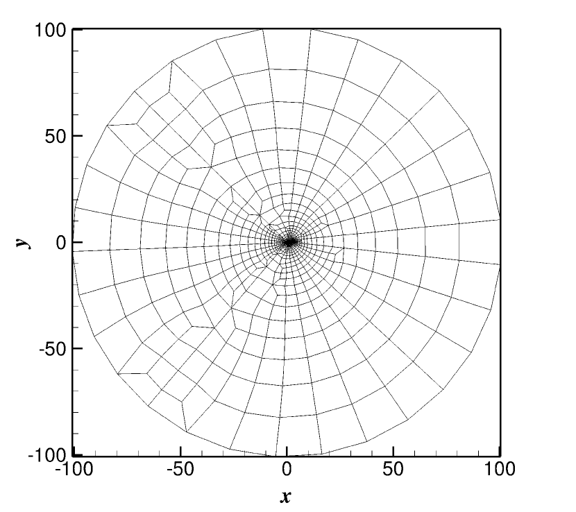
(a) Global view

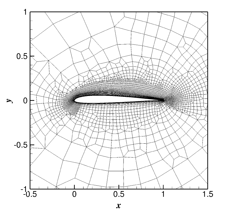
(b) Close-up view

Figure 10: 2D views of the unstructured mesh around the SD7003 wing.

In this section, we apply the $p$-adaptive solver to the simulation of the transitional flow over the SD7003 wing. The geometry of the wing is obtained from the $1^{\text{st}}$ International Workshop on High-Order CFD Methods. The chord length of the wing is $c=1$ with the sharp trailing edge rounded by an arc of radius $r\approx 0.0004$. The inflow conditions are $(\rho_{\infty},u_{\infty},v_{\infty},w_{\infty},\text{Ma}_{\infty})^{\intercal}=(1,1,0,0,0.1)^{\intercal}$. The angle of attack of the inflow is $8^{\circ}$. The Reynolds number of the inflow with respect to the chord length of the wing is $\text{Re}_{c}={\rho_{\infty}u_{\infty}c}/{\mu}=60000$. The Prandtl number is $\text{Pr}=0.72$. 2D views of the unstructured mesh used for under-resolved simulation are illustrated in Figure 10. The height of the first layer of elements in the normal direction of the wing is $0.0003c$. We extrude the 2D mesh along the $z$ direction to obtain the 3D mesh. The first 3D mesh has 20 layers in the $z$ direction and 109,540 hexahedral elements in total. The thickness of each layer is $0.01c$. The second one has ten layers in the spanwise direction and each layer has a thickness of $0.02c$. Taking advantage of $p$-adaptation, only the $p$-adaptive $p^{2}$ and $p^{3}$ FR methods are used to simulate this problem. We will provide the reduction in the total number of solution points $n_{sp}^{tot}$ to demonstrate the efficiency of $p$-adaptation. The $p$-adaptation parameters are set as $(\nu_{max},\nu_{min})=(0.1,0.001)$.

The time step $\Delta t=0.002$ and tolerance for the pseudo transient continuation $tol_{rel}^{pseudo}=10^{-4}$ are employed for all numerical experiments. For the simulation on the 20-layer mesh, ESDIRK2 is employed for time integration with $tol_{rel}^{gmres}=10^{-1}$ for the GMRES solver. In the pseudo transient continuation, $\Delta\tau_{min}=0.0002$ and $\Delta\tau_{max}=0.004$ are used for SER. We first run the simulation with adaptive $p^{2}$ FR until $t_{1}=26$. The instantaneous values of conservative variables in $t\in(20,26]$ are used for averaging. Then we increase the $p_{max}$ to $p_{max}=3$ and resume the simulation until $t_{2}=42$. Then, averaging is done for $t\in(36,42]$. When $p^{3}$ FR with $p$-adaptation is used to simulate this problem on the 10-layer mesh, aliasing errors will lead to failure. Therefore, we employ a simple nodal polynomial filtering method proposed by Fisher and Mullen [35] for every element whose polynomial degree exceeds two. The $p^{2}$ polynomial is employed as a basis to perform a cut-off as $\widetilde{\boldsymbol{q}}_{p^{3}}=(1-\alpha)\boldsymbol{q}_{p^{3}}+\alpha\mathbb{P}_{p^{2}}^{p^{3}}\boldsymbol{q}_{p^{3}}$, where $\mathbb{P}_{p^{2}}^{p^{3}}$ is the projection operation from $p^{3}$ to $p^{2}$ and $\alpha=0.2$. With this nodal polynomial filtering, a small amount of dissipation is introduced to stabilize the numerical methods. ESDIRK4 serves as the time integrator for the simulation on the 10-layer mesh with adaptive $p^{3}$ FR. To increase the robustness of the pseudo transient continuation, $tol_{rel}^{gmres}=10^{-2}$, $\Delta\tau_{min}=0.0002$, and $\Delta\tau_{max}=0.002$ are used. We run the simulation until $t_{1}=26$ only. Solutions in $t\in(20,26]$ are averaged for statistics.

Two snapshots of the instantaneous isosurfaces of the $Q$-criterion, where $Q=500$, are presented in Figure 11 for the simulation conducted on the 20-layer mesh. One visible difference is that more finer structures are resolved using adaptive $p^{3}$ FR. From Figure 12 and Figure 13, we observe that polynomials of degree $p>1$ are clustered in regions near the stagnation point, turbulent boundary layers as well as the wake region. The order-of-accuracy distributions at different slices in the spanwise direction are not exactly the same since the $p$-adaptation is conducted locally. Overall, the feature-based adaptation method can give an feature-tracking $p$-distribution. Unlike the transitional flow over the cylinder, the choice of $(\nu_{max},\nu_{min})=(0.1,0.001)$ actually clusters all the polynomials of degree $p>1$ in a small domain and only a few high-order elements can be found in the wake region far away from the wing. The power spectral density of the total velocity at four locations close to the suction side of the wing, i.e., $(0.3,0.057,0.1)^{\intercal}$ $(0.5,0.048,0.1)^{\intercal}$, $(0.7,0.032,0.1)^{\intercal}$, and $(0.9,0.012,0.1)^{\intercal}$ are illustrated in Figure 14. The first point is near the end of the separation bubble, where the transition from laminar flow to turbulent flow takes place. The slopes of PSDs are generally steeper than $-5/3$ at high frequencies at the first point in all simulation. At the rest three points, PSDs align with the reference lines in a certain range of high frequencies, which agrees with the results in [67].

The mean field of the averaged velocity component $u$ in the $x$ direction are presented in Figure 15. Predictions of the time-averaged flow features, namely, lift coefficient $C_{l}$, drag coefficient $C_{d}$, separation point $x_{s}$, and reattachment point $x_{re}$, are documented in Table 2. The reduction of the total number of solution points $n_{sp}^{tot}$ at specific time instances are also provided in Table 2. The time-averaged surface pressure coefficient $C_{p}$ and surface friction coefficient $C_{f}$ on the SD7003 wing are illustrated in Figure 16. All numerical experiments over-predict the drag when compared to the experimental result [68]. Simulation of the incompressible Navier–Stokes equations done by Bassi et al. [52] gave larger $C_{d}$ than those of the compressible Navier–Stokes equations when $\text{Ma}=0.1$. The numerical results of our current work have a decent agreement with those in [69]. For simulation conducted on the 20-layer mesh, the adaptive $p^{2}$ FR has 1,644,414 solution points at $t_{1}=26$; the adaptive $p^{3}$ FR has 2,570,297 solution points at $t_{2}=42$. The reductions compared to $p$-uniform $p^{2}$ and $p^{3}$ FR are 44.40% and 63.34%, respectively. The reduction of solution points on the 10-layer mesh using $p$-adaptive $p^{3}$ FR is 60.57% at $t_{1}=26$. From the reduction in the total number of solution points, we can speculate a similar reduction in the computational cost or run time. We note that insufficient resolution of the physical scales will lead to failure of the under-resolved turbulence simulation due to insufficient grid resolution in the 10-layer mesh. However, with a small dissipation introduced by nodal polynomial filtering, the force prediction can be accurate to 0.01 and the length of separation bubble is only slightly shorter. It is hard to know whether one under-resolved turbulence simulation will fail due to aliasing errors. Therefore, in the practice of performing under-resolved turbulence simulation using high-order methods, we would recommend to employ proper de-aliasing techniques.

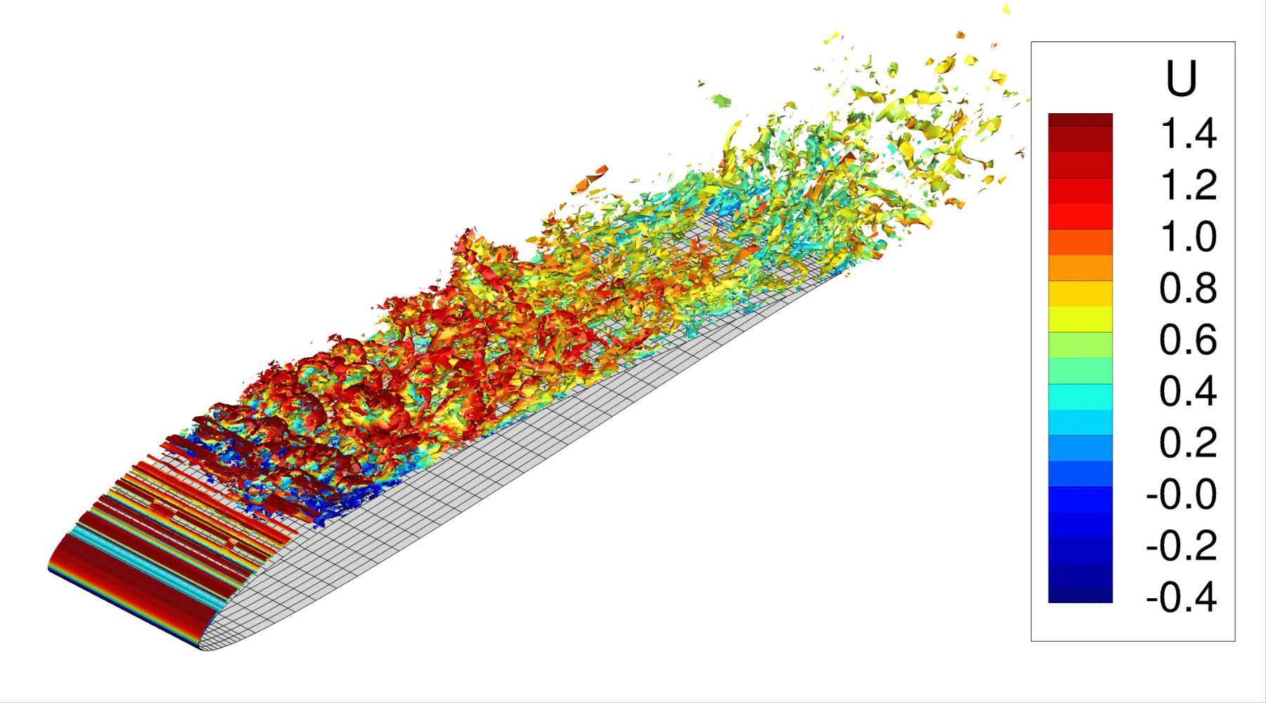
(a) Adaptive $p^{2}$ FR, $t=26$

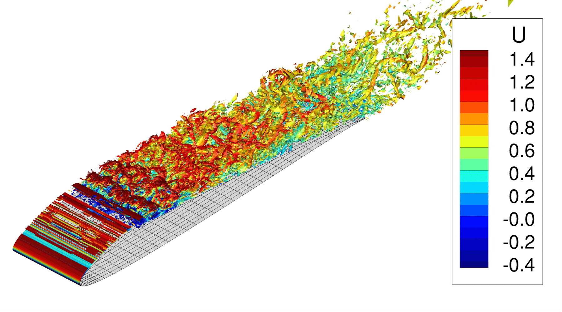
(b) Adaptive $p^{3}$ FR, $t=40$

Figure 11: Instantaneous $Q$-isosurfaces colored by velocity component $u$ in the $x$ direction when simulating the transitional flow on the 20-layer mesh.

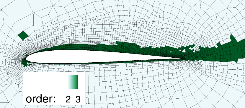
(a) $z=0.05$

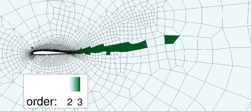
(b) $z=0.05$

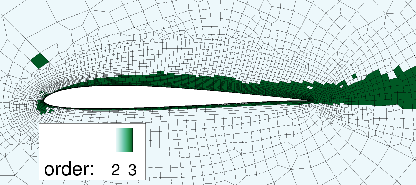
(c) $z=0.1$

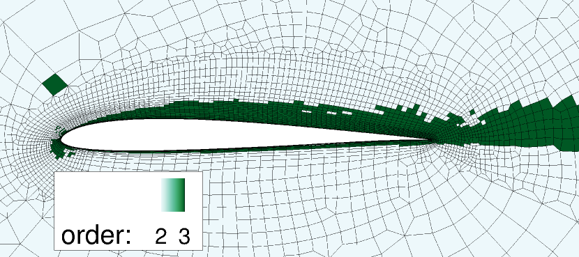
(d) $z=0.15$

Figure 12: Instantaneous order-of-accuracy distributions of adaptive $p^{2}$ FR at different slices in the spanwise direction when simulating the transitional flow over the SD7003 wing. $t=26$.

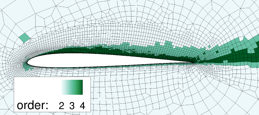
(a) $z=0.05$

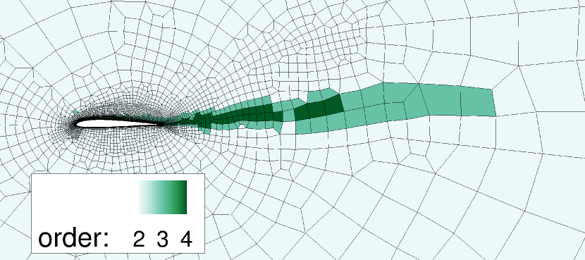
(b) $z=0.15$

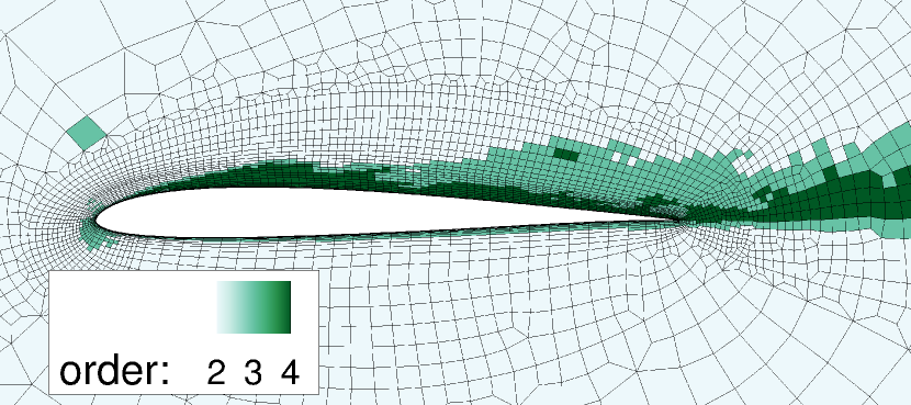
(c) $z=0.1$

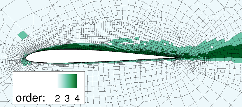
(d) $z=0.15$

Figure 13: Instantaneous order-of-accuracy distributions of adaptive $p^{3}$ FR at different slices in the spanwise direction when simulating the transitional flow over the SD7003 wing. $t=40$.

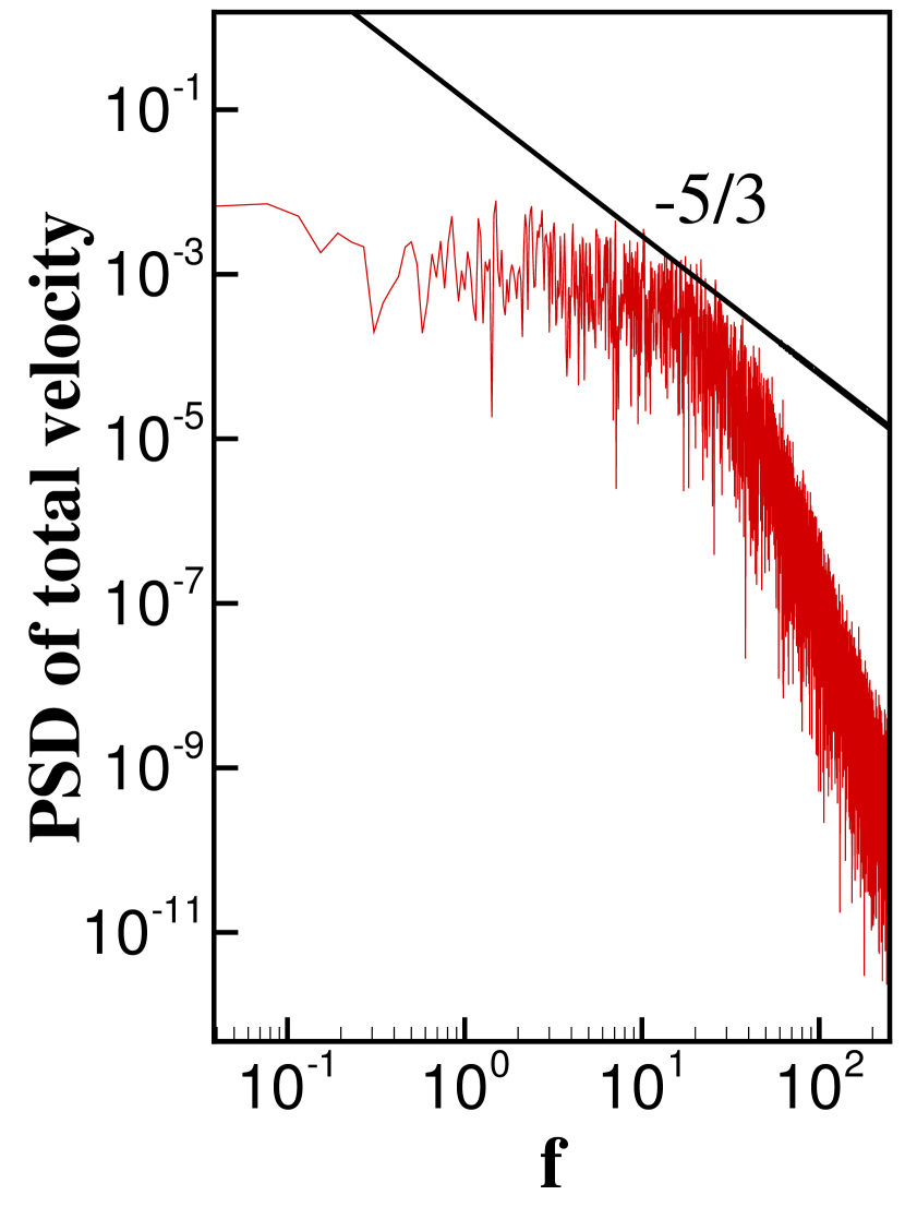
(a) $(0.3,0.057,0.1)^{\intercal}$

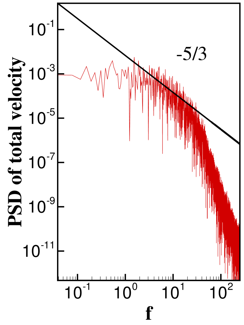
(b) $(0.5,0.048,0.1)^{\intercal}$

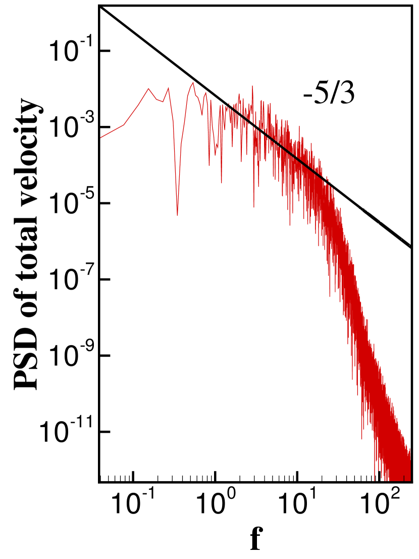
(c) $(0.7,0.032,0.1)^{\intercal}$

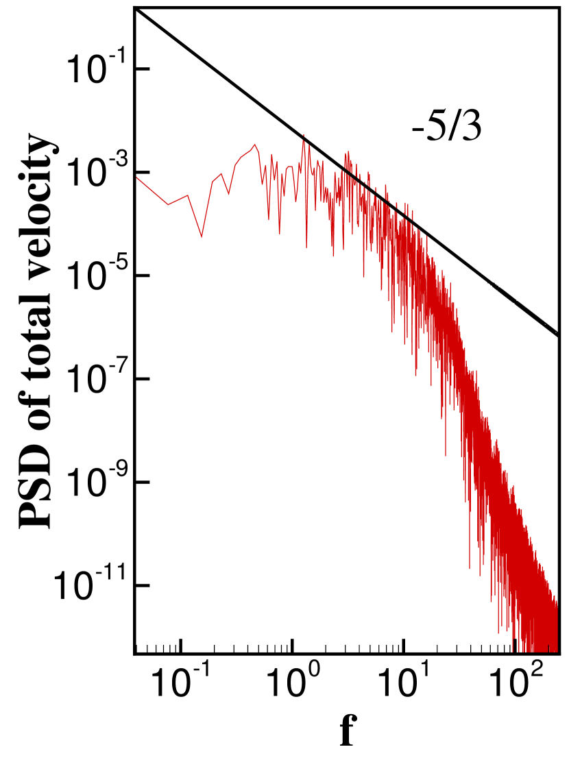
(d) $(0.9,0.012,0.1)^{\intercal}$

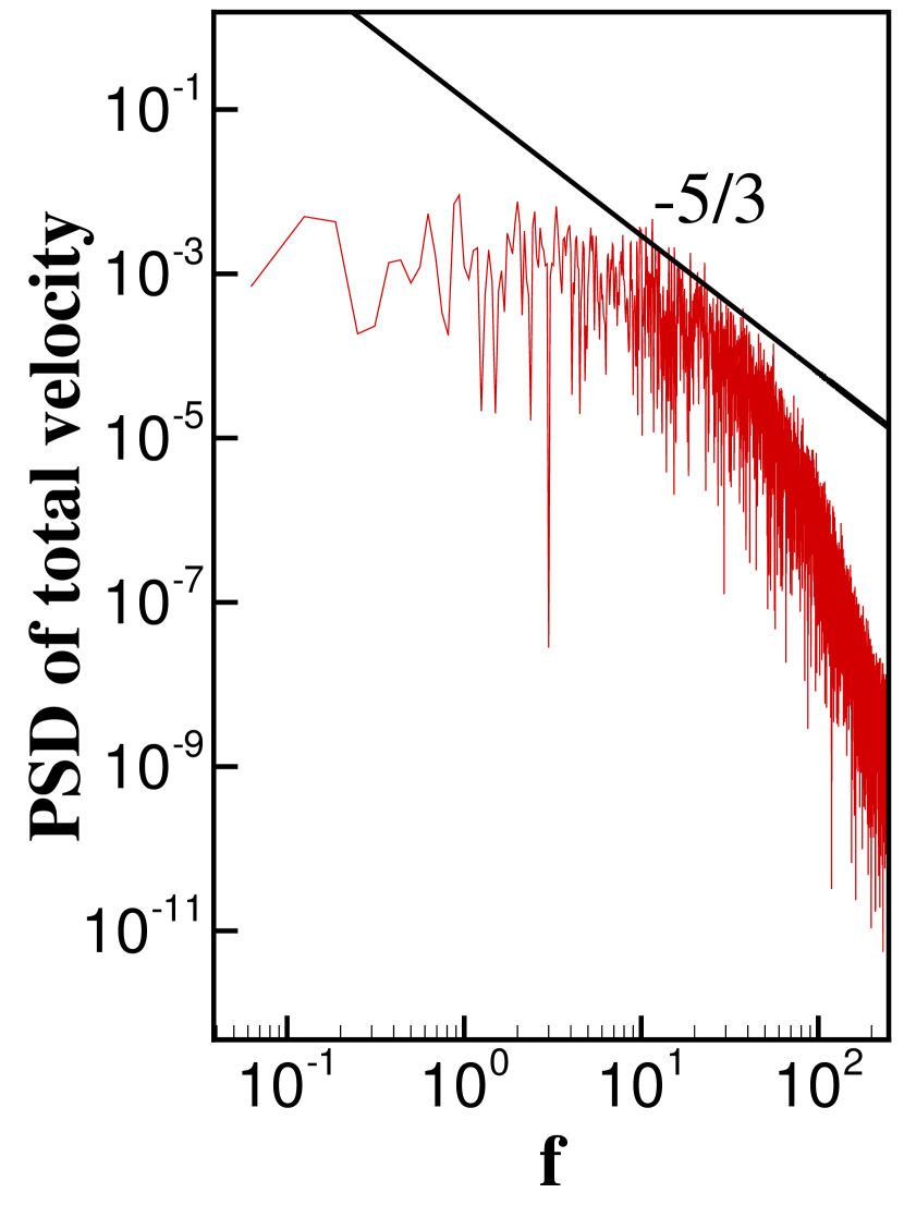
(e) $(0.3,0.057,0.1)^{\intercal}$

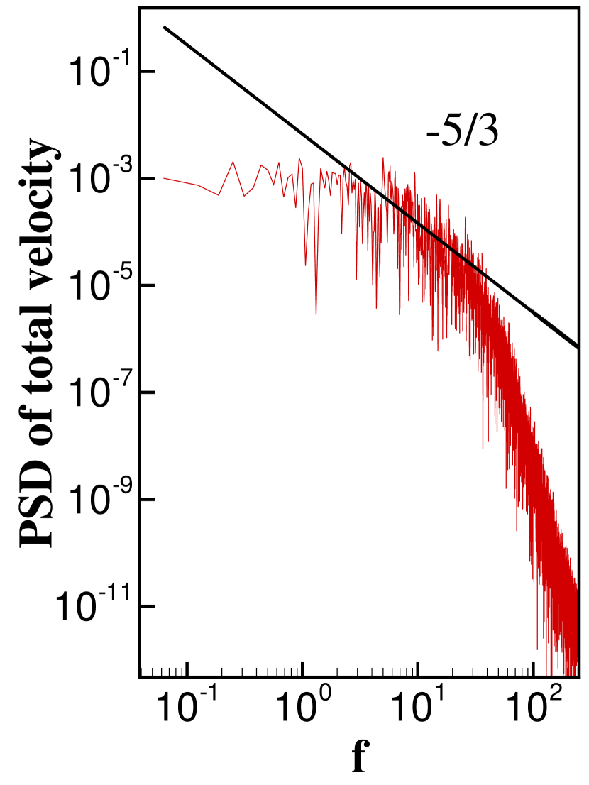
(f) $(0.5,0.048,0.1)^{\intercal}$

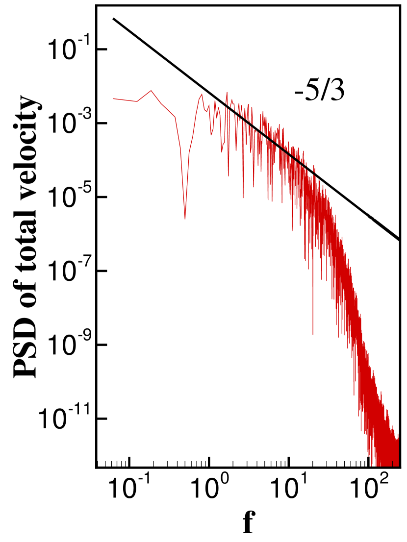
(g) $(0.7,0.032,0.1)^{\intercal}$

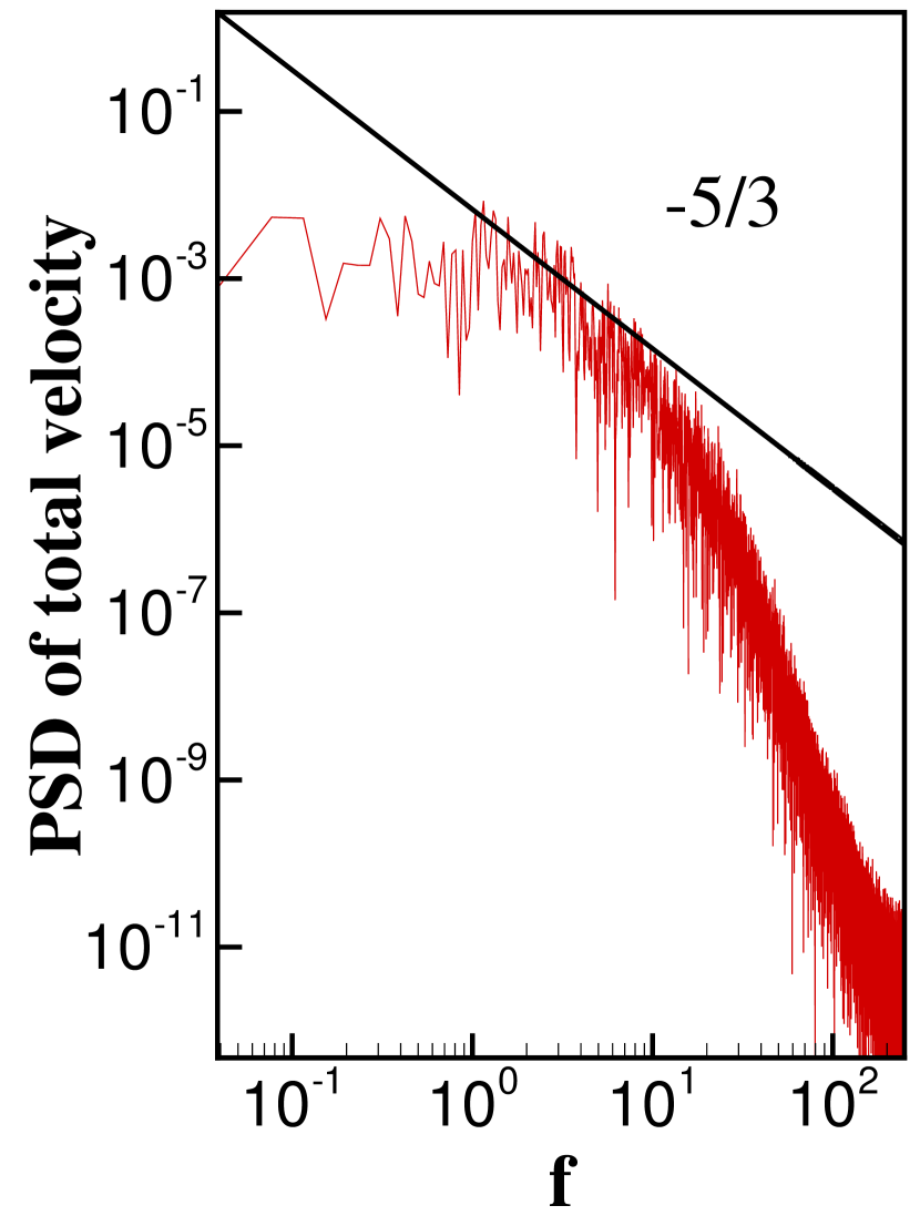
(h) $(0.9,0.012,0.1)^{\intercal}$

Figure 14: Power spectral density of the total velocity at different locations in the wake region. (a)–(d) $p^{3}$ FR with no adaptation and (e)–(h) adaptive $p^{3}$ FR with $(\nu_{max},\nu_{min})=(0.1,0.01)$. A line of slope $-5/3$ is added to every graph as a reference.

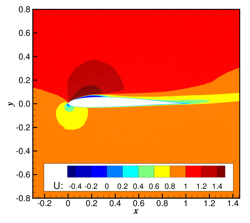
(a) $p^{2}$ FR with adaptation

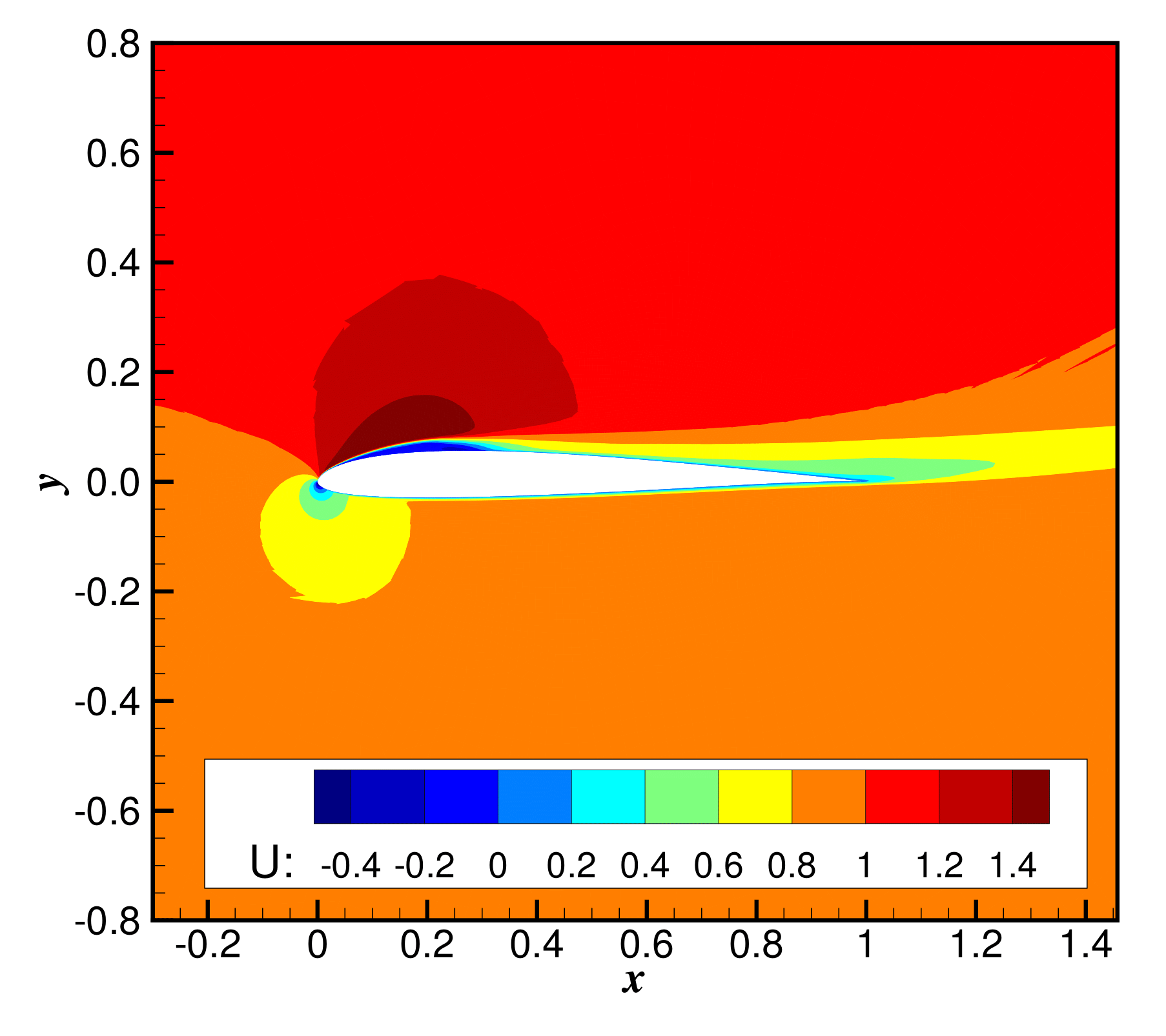
(b) $p^{3}$ FR with adaptation

Figure 15: Averaged velocity component in the $x$ direction on the 20-layer mesh.

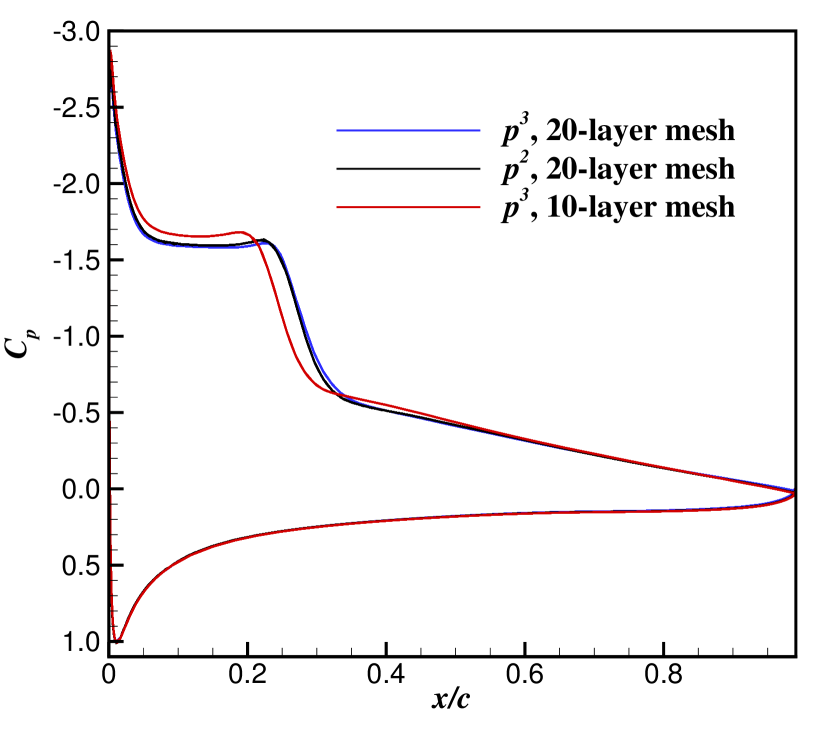
(a) $C_{p}$

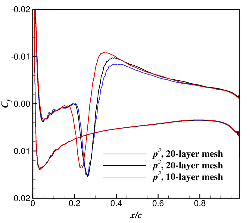
(b) $C_{f}$

Figure 16: Time-averaged surface pressure coefficient $C_{p}$ and surface friction coefficient $C_{f}$ on the SD7003 wing.

Table 2: Predictions of the transitional flow using the $p$-adaptive solver. Rows 1–3 are from current work using $p$-adaptive FR. Rows 4–9 are previous numerical results using $p$-uniform high-order methods. Row 10 presents the results from experiment. The abbreviation Inc. stands for “incompressible”.

	Spatial discretization	Ma	$C_{l}$	$C_{d}$	$x_{s}$	$x_{re}$	Reduction of $n_{sp}^{tot}$
1	$p$-adaptive, $p^{2}$ FR (20-layer)	0.1	0.9289	0.0459	0.0321	0.3075	44.40% at $t_{1}=26$
2	$p$-adaptive, $p^{3}$ FR (20-layer)	0.1	0.9270	0.0470	0.0301	0.3123	63.34% at $t_{2}=42$
3	$p$-adaptive, $p^{3}$ FR (10-layer)	0.1	0.9316	0.0419	0.0336	0.2735	60.57% at $t_{1}=26$
4	$p^{4}$ FR (Vermeire et al. [70])	0.2	0.941	0.049	0.045	0.315
5	$p^{3}$ DG (Beck et al. [69])	0.1	0.923	0.045	0.027	0.310
6	$p^{7}$ DG (Beck et al. [69])	0.1	0.932	0.050	0.030	0.336
7	$O(h^{6})$ FD (Galbriath & Visbal [13])	0.1	0.91	0.043	0.04	0.28
8	$p^{3}$ DG (Bassi et al. [52])	Inc.	0.962	0.042	0.027	0.268
9	$p^{4}$ DG (Bassi et al. [52])	Inc.	0.953	0.045	0.027	0.294
10	Experiment (Selig et al. [68])		0.92	0.029

5 Conclusion

In this work, a dynamically load balanced parallel $p$-adaptive implicit high-order flux reconstruction method is developed and applied to under-resolved turbulence simulation. The parallel mesh partitioning API in ParMETIS, i.e., ParMetis_V3_AdaptiveRepart(), is utilized for efficient parallel mesh partitioning. A collect-and-distribute strategy is used to redistribute the working variables to different processes. We have discussed the impact of weight calculation for each element on the parallel efficiency in the context of matrix-free implementation of the ESDIRK method. We investigate different weights related to the cost of residual evaluation, Jacobian matrix and preconditioner evaluation, and GMRES iterations. For $p\leq 3$, we recommend $\omega_{e}=n_{sp}$, and as $p$ grows larger, $\omega_{e}=n_{sp}^{k}$, where $k>1$, is more preferable. Overall, a significant reduction in the run time and total number of solution points can be achieved via $p$-adaptation for turbulence simulation and favorable results can be obtained.

When the adaptive solver is applied to solving the transitional flow over an infinite cylinder, due to the presence of large flow separation, the featured-based solver can result in a large domain where the polynomial degrees are refined. One can adjust the adaptation criteria towards wall-resolving to save computational cost; however, the accuracy would be compromised. When the flow separation is small, e.g., transitional flow over the SD7003 wing at a small angle of attack, the feature-based $p$-adaptation method is able to confine the $p$-refined region close to the wing, thus significantly reducing the cost while providing good predictions. We also show, with the SD7003 case, that insufficient mesh resolution can lead to instabilities triggered by aliasing errors of high-order methods in under-resolved turbulence simulation. A proper de-aliasing technique can overcome this issue and provide acceptable predictions.

The framework of dynamically load balanced $p$-adaptive implicit high-order methods developed in this study paves the way towards robust and efficient ILES of turbulent flows at higher Reynolds numbers with the high-order FR/CPR method. The dynamic load balancing technique presented here can be easily extended to other types of high-order collocation methods.

References

- [1] B. Cockburn and C.-W. Shu, “TVB Runge-Kutta local projection discontinuous Galerkin finite element method for conservation laws II: general framework,” Mathematics of Computation, vol. 52, pp. 411–435, 1989.
- [2] B. Cockburn, S. Hou, and C.-W. Shu, “The Runge-Kutta local projection discontinuous Galerkin finite element method for conservation laws. IV. The multidimensional case,” Mathematics of Computation, vol. 54, no. 190, pp. 545–581, 1990.
- [3] F. Bassi and S. Rebay, “A high-order accurate discontinuous finite element method for the numerical solution of the compressible Navier–Stokes equations,” Journal of Computational Physics, vol. 131, no. 2, pp. 267–279, 1997.
- [4] B. Cockburn and C.-W. Shu, “Runge–Kutta discontinuous Galerkin methods for convection-dominated problems,” Journal of Scientific Computing, vol. 16, no. 3, pp. 173–261, 2001.
- [5] F. Bassi, A. Crivellini, S. Rebay, and M. Savini, “Discontinuous Galerkin solution of the Reynolds-averaged Navier–Stokes and k– turbulence model equations,” Computers & Fluids, vol. 34, no. 4-5, pp. 507–540, 2005.
- [6] J. S. Hesthaven and T. Warburton, Nodal Discontinuous Galerkin Methods: Algorithms, Analysis, and Applications. New York: Springer-Verlag, 2008.
- [7] G. J. Gassner and A. D. Beck, “On the accuracy of high-order discretizations for underresolved turbulence simulations,” Theoretical and Computational Fluid Dynamics, vol. 27, no. 3-4, pp. 221–237, 2013.
- [8] A. Uranga, P.-O. Persson, M. Drela, and J. Peraire, “Implicit large eddy simulation of transition to turbulence at low Reynolds numbers using a discontinuous Galerkin method,” International Journal for Numerical Methods in Engineering, vol. 87, no. 1-5, pp. 232–261, 2011.
- [9] Y. Liu, M. Vinokur, and Z. J. Wang, “Spectral difference method for unstructured grids I: basic formulation,” Journal of Computational Physics, vol. 216, no. 2, pp. 780–801, 2006.
- [10] Y. Zhou and Z. J. Wang, “Implicit Large Eddy Simulation of Low Reynolds Number Transitional Flow over a Wing Using High-Order Spectral Difference Method,” in 40th Fluid Dynamics Conference and Exhibit, p. 4442, 2010.
- [11] P. Castonguay, C. Liang, and A. Jameson, “Simulation of transitional flow over airfoils using the spectral difference method,” in 40th Fluid Dynamics Conference and Exhibit, p. 4626, 2010.
- [12] M. L. Yu, Z. J. Wang and H. Hu, “A high-order spectral difference method for unstructured dynamic grids,” Computers & Fluids, vol. 48, pp. 84–97, 2011.
- [13] M. Galbraith and M. Visbal, “Implicit large eddy simulation of low Reynolds number flow past the SD7003 airfoil,” in 46th AIAA Aerospace Sciences Meeting and Exhibit, p. 225, 2008.
- [14] D. J. Garmann, M. R. Visbal, and P. D. Orkwis, “Comparative study of implicit and subgrid-scale model large-eddy simulation techniques for low-Reynolds number airfoil applications,” International Journal for Numerical Methods in Fluids, vol. 71, no. 12, pp. 1546–1565, 2013.
- [15] P. Boom and D. Zingg, “Time-accurate flow simulations using an efficient newton-krylov-schur approach with high-order temporal and spatial discretization,” in 51st AIAA Aerospace Sciences Meeting including the New Horizons Forum and Aerospace Exposition, p. 383, 2013.
- [16] M. H. Carpenter, T. C. Fisher, E. J. Nielsen, and S. H. Frankel, “Entropy Stable Spectral Collocation Schemes for the Navier–Stokes Equations: Discontinuous Interfaces,” SIAM Journal on Scientific Computing, vol. 36, no. 5, pp. B835–B867, 2014.
- [17] M. Svärd and J. Nordström, “Review of summation-by-parts schemes for initial–boundary-value problems,” Journal of Computational Physics, vol. 268, pp. 17–38, 2014.
- [18] H. T. Huynh, “A flux reconstruction approach to high-order schemes including discontinuous Galerkin methods,” in 18th AIAA Computational Fluid Dynamics Conference, p. 4079, 2007.
- [19] H. T. Huynh, “A Reconstruction Approach to High-Order Schemnes Including Discontinuous Galerkin for Diffusion,” in 47th AIAA Aerospace Sciences Meeting Including The New Horizons Forum and Aerospace Exposition, p. 403, 2009.
- [20] Z. J. Wang and H. Gao, “A unifying lifting collocation penalty formulation including the discontinuous Galerkin, spectral volume/difference methods for conservation laws on mixed grids,” Journal of Computational Physics, vol. 228, no. 21, pp. 8161–8186, 2009.
- [21] P. E. Vincent, P. Castonguay, and A. Jameson, “A new class of high-order energy stable flux reconstruction schemes,” Journal of Scientific Computing, vol. 47, no. 1, pp. 50–72, 2011.
- [22] J. Romero, K. Asthana, and A. Jameson, “A simplified formulation of the flux reconstruction method,” Journal of Scientific Computing, vol. 67, no. 1, pp. 351–374, 2016.
- [23] L. Wang and M. Yu, “Compact direct flux reconstruction for conservation laws,” Journal of Scientific Computing, pp. 1–23, 2017.
- [24] F. D. Witherden, A. M. Farrington, and P. E. Vincent, “PyFR: An open source framework for solving advection–diffusion type problems on streaming architectures using the flux reconstruction approach,” Computer Physics Communications, vol. 185, no. 11, pp. 3028–3040, 2014.
- [25] P. Fernandez, N.-C. Nguyen, and J. Peraire, “Subgrid-scale modeling and implicit numerical dissipation in DG-based Large-Eddy Simulation,” in 23rd AIAA Computational Fluid Dynamics Conference, p. 3951, 2017.
- [26] G. J. Gassner, “A skew-symmetric discontinuous Galerkin spectral element discretization and its relation to SBP-SAT finite difference methods,” SIAM Journal on Scientific Computing, vol. 35, no. 3, pp. A1233–A1253, 2013.
- [27] G. J. Gassner, A. R. Winters, and D. A. Kopriva, “Split form nodal discontinuous Galerkin schemes with summation-by-parts property for the compressible Euler equations,” Journal of Computational Physics, vol. 327, pp. 39–66, 2016.
- [28] R. M. Kirby and G. E. Karniadakis, “De-aliasing on non-uniform grids: algorithms and applications,” Journal of Computational Physics, vol. 191, no. 1, pp. 249–264, 2003.
- [29] G. Mengaldo, D. De Grazia, D. Moxey, P. E. Vincent, and S. J. Sherwin, “Dealiasing techniques for high-order spectral element methods on regular and irregular grids,” Journal of Computational Physics, vol. 299, pp. 56–81, 2015.
- [30] E. Tadmor, “Convergence of spectral methods for nonlinear conservation laws,” SIAM Journal on Numerical Analysis, vol. 26, no. 1, pp. 30–44, 1989.
- [31] G. Karamanos and G. E. Karniadakis, “A spectral vanishing viscosity method for large-eddy simulations,” Journal of Computational Physics, vol. 163, no. 1, pp. 22–50, 2000.
- [32] R. Pasquetti, “Spectral vanishing viscosity method for large-eddy simulation of turbulent flows,” Journal of Scientific Computing, vol. 27, no. 1-3, pp. 365–375, 2006.
- [33] D. Gottlieb and J. S. Hesthaven, “Spectral methods for hyperbolic problems,” Journal of Computational and Applied Mathematics, vol. 128, no. 1-2, pp. 83–131, 2001.
- [34] J. Hesthaven and R. Kirby, “Filtering in Legendre spectral methods,” Mathematics of Computation, vol. 77, no. 263, pp. 1425–1452, 2008.
- [35] P. Fischer and J. Mullen, “Filter-based stabilization of spectral element methods,” Comptes Rendus de l’Académie des Sciences-Series I-Mathematics, vol. 332, no. 3, pp. 265–270, 2001.
- [36] G. Gassner, M. Staudenmaier, F. Hindenlang, M. Atak, and C.-D. Munz, “A space–time adaptive discontinuous Galerkin scheme,” Computers & Fluids, vol. 117, pp. 247–261, 2015.
- [37] M. Tugnoli, A. Abbà, L. Bonaventura, and M. Restelli, “A locally p-adaptive approach for Large Eddy Simulation of compressible flows in a DG framework,” Journal of Computational Physics, vol. 349, pp. 33–58, 2017.
- [38] F. Naddei, M. de la Llave Plata, and V. Couaillier, “A comparison of refinement indicators for -adaptive discontinuous Galerkin methods for the Euler and Navier–Stokes equations,” in 2018 AIAA Aerospace Sciences Meeting, p. 0368, 2018.
- [39] R. Hartmann and P. Houston, “Adaptive discontinuous Galerkin finite element methods for the compressible Euler equations,” Journal of Computational Physics, vol. 183, no. 2, pp. 508–532, 2002.
- [40] H. Gao and Z. Wang, “A Residual-Based Procedure for Hp-Adaptation on 2-D Hybrid Meshes,” in 49th AIAA Aerospace Sciences Meeting including the New Horizons Forum and Aerospace Exposition, p. 492, 2011.
- [41] M. Kompenhans, G. Rubio, E. Ferrer, and E. Valero, “Comparisons of p-adaptation strategies based on truncation-and discretisation-errors for high order discontinuous Galerkin methods,” Computers & Fluids, vol. 139, pp. 36–46, 2016.
- [42] D. A. Venditti and D. L. Darmofal, “Anisotropic grid adaptation for functional outputs: application to two-dimensional viscous flows,” Journal of Computational Physics, vol. 187, no. 1, pp. 22–46, 2003.
- [43] L. Wang and D. J. Mavriplis, “Adjoint-based h–p adaptive discontinuous Galerkin methods for the 2D compressible Euler equations,” Journal of Computational Physics, vol. 228, no. 20, pp. 7643–7661, 2009.
- [44] K. J. Fidkowski and D. L. Darmofal, “Review of output-based error estimation and mesh adaptation in computational fluid dynamics,” AIAA Journal, vol. 49, no. 4, pp. 673–694, 2011.
- [45] K. J. Fidkowski and Y. Luo, “Output-based space–time mesh adaptation for the compressible Navier–Stokes equations,” Journal of Computational Physics, vol. 230, no. 14, pp. 5753–5773, 2011.
- [46] F. Bassi, A. Colombo, A. Crivellini, K. Fidkowski, M. Franciolini, A. Ghidoni, and G. Noventa, “An entropy-adjoint p-adaptive discontinuous Galerkin method for the under-resolved simulation of turbulent flows,” in AIAA Aviation 2019 Forum, p. 3418, 2019.
- [47] K. J. Fidkowski and P. L. Roe, “An entropy adjoint approach to mesh refinement,” SIAM Journal on Scientific Computing, vol. 32, no. 3, pp. 1261–1287, 2010.
- [48] P.-O. Persson and J. Peraire, “Sub-cell shock capturing for discontinuous Galerkin methods,” in 44th AIAA Aerospace Sciences Meeting and Exhibit, p. 112, 2006.
- [49] B. Cockburn and C.-W. Shu, “TVB Runge-Kutta local projection discontinuous Galerkin finite element method for conservation laws. II. General framework,” Mathematics of Computation, vol. 52, no. 186, pp. 411–435, 1989.
- [50] S. Gottlieb, C.-W. Shu, and E. Tadmor, “Strong stability-preserving high-order time discretization methods,” SIAM Review, vol. 43, no. 1, pp. 89–112, 2001.
- [51] C. A. Kennedy and M. H. Carpenter, “Diagonally implicit Runge-Kutta methods for ordinary differential equations. A review,” 2016.
- [52] F. Bassi, L. Botti, A. Colombo, A. Ghidoni, and F. Massa, “Linearly implicit Rosenbrock-type Runge–Kutta schemes applied to the Discontinuous Galerkin solution of compressible and incompressible unsteady flows,” Computers & Fluids, vol. 118, pp. 305–320, 2015.
- [53] L. Wang and M. Yu, “A comparative study of implicit Jacobian-free Rosenbrock-Wanner, ESDIRK and BDF methods for unsteady flow simulation with high-order flux reconstruction formulations,” arXiv preprint arXiv:1904.04825, 2019.
- [54] M. Franciolini, A. Crivellini, and A. Nigro, “On the efficiency of a matrix-free linearly implicit time integration strategy for high-order discontinuous Galerkin solutions of incompressible turbulent flows,” Computers & Fluids, vol. 159, pp. 276–294, 2017.
- [55] D. A. Knoll and D. E. Keyes, “Jacobian-free Newton–Krylov methods: a survey of approaches and applications,” Journal of Computational Physics, vol. 193, no. 2, pp. 357–397, 2004.
- [56] L. Wang and M. Yu, “Jacobian-free implicit p-adaptive high-order compact direct flux reconstruction methods for unsteady flow simulation,” in AIAA Aviation 2019 Forum, p. 3062, 2019.
- [57] G. Karypis, “METIS and ParMETIS,” Encyclopedia of Parallel Computing, pp. 1117–1124, 2011.
- [58] M. Yu and Z. J. Wang, “On the connection between the correction and weighting functions in the correction procedure via reconstruction method,” Journal of Scientific Computing, vol. 54, no. 1, pp. 227–244, 2013.
- [59] D. M. Williams, P. Castonguay, P. E. Vincent, and A. Jameson, “Energy stable flux reconstruction schemes for advection–diffusion problems on triangles,” Journal of Computational Physics, vol. 250, pp. 53–76, 2013.
- [60] P. L. Roe, “Approximate Riemann solvers, parameter vectors, and difference schemes,” Journal of Computational Physics, vol. 43, no. 2, pp. 357–372, 1981.
- [61] H. Bijl, M. H. Carpenter, V. N. Vatsa, and C. A. Kennedy, “Implicit time integration schemes for the unsteady compressible Navier–Stokes equations: laminar flow,” Journal of Computational Physics, vol. 179, no. 1, pp. 313–329, 2002.
- [62] W. A. Mulder and B. Van Leer, “Experiments with implicit upwind methods for the Euler equations,” Journal of Computational Physics, vol. 59, no. 2, pp. 232–246, 1985.
- [63] S. Balay, S. Abhyankar, M. F. Adams, J. Brown, P. Brune, K. Buschelman, L. Dalcin, V. Eijkhout, W. D. Gropp, D. Kaushik, M. G. Knepley, L. C. McInnes, K. Rupp, B. F. Smith, S. Zampini, and H. Zhang, “PETSc users manual,” Tech. Rep. ANL-95/11 - Revision 3.6, Argonne National Laboratory, 2015.
- [64] L. Wang and M. Yu, “An Implicit High-Order Preconditioned Flux Reconstruction Method for Low-Mach-Number Flow Simulation with Dynamic Meshes,” International Journal for Numerical Methods in Fluids, 2019.
- [65] L. Wang and M. Yu, “An implicit -multigrid flux reconstruction method for simulation of locally preconditioned unsteady Navier-Stokes equations at low Mach numbers,” arXiv preprint arXiv:1908.03972, 2019.
- [66] O. Lehmkuhl, I. Rodríguez, R. Borrell, and A. Oliva, “Low-frequency unsteadiness in the vortex formation region of a circular cylinder,” Physics of Fluids, vol. 25, no. 8, p. 085109, 2013.
- [67] F. Bassi, L. Botti, A. Colombo, A. Crivellini, A. Ghidoni, and F. Massa, “On the development of an implicit high-order Discontinuous Galerkin method for DNS and implicit LES of turbulent flows,” European Journal of Mechanics-B/Fluids, vol. 55, pp. 367–379, 2016.
- [68] M. S. Selig, Summary of low speed airfoil data Vol. 1. SoarTech Publications, 1995.
- [69] A. D. Beck, T. Bolemann, D. Flad, H. Frank, G. J. Gassner, F. Hindenlang, and C.-D. Munz, “High-order discontinuous Galerkin spectral element methods for transitional and turbulent flow simulations,” International Journal for Numerical Methods in Fluids, vol. 76, no. 8, pp. 522–548, 2014.
- [70] B. C. Vermeire, F. D. Witherden, and P. E. Vincent, “On the utility of GPU accelerated high-order methods for unsteady flow simulations: A comparison with industry-standard tools,” Journal of Computational Physics, vol. 334, pp. 497–521, 2017.