SCHWINGER-BASED QCD FORMULATION’S DERIVATION OF ELASTIC PP SCATTERING

Abstract

Using previously described functional techniques for some non-perturbative, gauge invariant, renormalized QCD processes, a simplified version of the amplitudes - in which forms akin to Pomerons naturally appear - provides fits to ISR and LHC-TOTEM pp elastic scattering data. Those amplitudes rely on a specific function $\phi(b)$ which describes the fluctuations of the transverse position of quarks inside hadrons.

1 Introduction

This talk is covers the work in  [1]. Beginning with Schwinger’s Generating Functional and the QCD Lagrangian, applying two procedures that were overlooked in the last four decades, an analytic, gauge-invariant correlation functions for Non-Perturbative QCD is obtained. This formulation produces the following results thus far:

• First-principled dynamical quark confining potential for quarks [2],

• A potential obtained from QCD that allows nucleons to be bounded, thus provided the first-principled model deuteron [3],

• New property of Effective Locality, provides gauge-invariant summation of all gluonic exchanges between quarks; more over, the interaction becomes a local interaction. [4].

• Obtained Chiral Symmetry Breaking for dynamical quarks out of the new property of Effective Locality [5].

• Extended Asymptotic freedom as supported by other non-perturbative approaches: Dyson Schwinger Equation [6].

• A qualitative description of the Hadron Confinement mass scale(s) [7].

• The full SU(3) algebraic content of QCD amplitudes, both $C_{2}$ and $C_{3}$ casimir invariants are preserved [8].

• First-principled calculation of elastic proton-proton scattering at ISR and LHC energies. This will be the focus of this talk [1].

1.1 Schwinger Generating Functional

The Schwinger Generating Functional can be rewritten into gaussian operations on gaussian fields.

$$\mathfrak{Z}_{QCD}[\bar{\eta},\eta,j]=\mathfrak{N}e^{-\frac{i}{2}\int\frac{\partial}{\partial A}\cdot D_{F}^{(0)}\cdot\frac{\partial}{\partial A}}\cdot e^{\frac{i}{4}\int\bf{F}^{2}+\frac{i}{2}\int A\cdot(-\partial^{2})\cdot A}\cdot e^{i\int\bar{\eta}\cdot\bf{G}_{F}[A]\cdot\eta+\bf{L}[A]}|_{A=\int D_{F}^{(0)}\cdot j}$$ (1)

where $G_{F}(x,y|A)=[m+\gamma\cdot(\delta-igA\tau)]^{-1}$, and $L[A]=ln[1-i\gamma A\tau[0]]$.

The $\bf{F}^{2}$ can be linearized with Halpern’s half a century old expression:

$$e^{-\frac{i}{4}\int\bf{F}^{2}}=N\int d[\chi]e^{\frac{i}{4}\int\chi^{2}+\frac{i}{2}\int F\cdot\chi}\scriptstyle$$ (2)

where $\chi^{a}_{\mu\nu}=-\chi^{a}_{\nu\mu}$ is anti symmetric tensor. It is this added $\chi$ field that plays the central role in the summation of all gluons in the non-perturbative regime.

1.2 Gauge-Invariance

Schwinger’s Generating Functional now becomes

$$\mathfrak{Z}_{QCD}[\bar{\eta},\eta,j]=N\int d[\chi]e^{\frac{i}{4}\int\chi^{2}}e^{\mathfrak{D}_{A}^{(0)}}\cdot e^{\frac{i}{2}\int\chi\cdot\bf{F}+\frac{i}{2}\int A\cdot(-\partial)\cdot A}e^{i\int\bar{\eta}\cdot G_{F}[A]\cdot\eta+L[A]}|_{A=\int D_{F}^{(0)}\cdot j}$$ (3)

Calculating 2n-point Fermionic Green’s functions (e.g. n=2), gives

$$=N\int d[\chi]e^{\frac{i}{4}\int\chi^{2}}e^{\mathfrak{D}_{A}^{(0)}}e^{\frac{i}{2}\int A\cdot(D_{F}^{(0)})^{-1}\cdot A}G_{F}(1|gA)G_{F}(2|gA)e^{L[A]}|_{A=0}$$ (4)

$$e^{\mathfrak{D_{a}}}F_{1}[A]=exp[\frac{i}{2}\int\bar{Q}\cdot D_{F}^{(0)}\cdot(1-\bar{K}\cdot D_{F}^{(0)})^{-1}\cdot\bar{Q}-\frac{1}{2}Tr\ln(1-D_{F}\cdot\tilde{K}]\cdot exp[\frac{1}{2}\int A\cdot\bar{K}\cdot(1-D_{F}^{(0)}\cdot\bar{K})^{-1}\cdot A]$$ (5)

where

$$D_{F}^{(0)}\cdot(1-\bar{K}\cdot D_{F}^{(0)})^{-1}=D_{F}^{(0)}\cdot[1-\hat{K}+(D_{F}^{(0)})^{-1})\cdot D_{F}^{(0)}]^{-1}=-(\tilde{K}_{\mu\nu}^{ab}+gf^{abc}\chi_{\mu\nu}^{c})^{-1}=-\hat{\bf{K}}^{-1}$$ (6)

with $F_{1}[A]=e^{\frac{i}{2}\int A\cdot\bar{K}\cdot A+i\int\bar{Q}\cdot A}$, $F_{2}[A]=e^{L[A]}$ and $<z|\bar{K}_{\mu\nu}^{ab}|z^{\prime}>=[\tilde{\bf{K}}^{ab}_{\mu\nu}(z)+gf^{abc}\chi_{\mu\nu}^{c}(z)]\delta^{(4)}(z-z^{\prime})+<z|(D_{F}^{(0)})^{-1}|_{\mu\nu}^{ab}|z^{\prime}>$.

We then have

$$e^{\mathfrak{D}_{A}}F_{1}[A]F_{2}[A]=exp[-\frac{i}{2}\int\bar{Q}\cdot\hat{K}^{-1}\cdot\bar{Q}]+\frac{1}{2}Tr\ln\hat{\bf{K}}+\frac{1}{2}Tr\ln(-D_{F}^{(0)})]\\ \cdot exp[\frac{i}{2}\int\frac{\partial}{\partial A}\cdot D_{F}^{(0)}\cdot\frac{\partial}{\partial A^{\prime}}]\cdot exp[\frac{i}{2}\int\frac{\partial}{\partial A^{\prime}}\cdot\hat{\bf{K}}^{-1}\cdot\frac{\partial}{\partial A^{\prime}}-\int\bar{Q}\cdot\hat{\bf{K}}^{-1}\cdot\frac{\partial}{\partial A^{\prime}}]\cdot(e^{\mathfrak{D}_{A}}F_{2}[A^{\prime}])$$ (7)

and

$$e^{\mathfrak{D}_{A}}F_{1}[A]F_{2}[A]=Nexp[-\frac{i}{2}\int\bar{Q}\cdot\hat{\bf{K}}^{-1}\cdot\bar{Q}+\frac{1}{2}Tr\ln\hat{\bf{K}}]\cdot exp[\frac{i}{2}\int\frac{\partial}{\partial A}\cdot\hat{\bf{K}}^{-1}\cdot\frac{\partial}{\partial A}-\int\bar{Q}\cdot\hat{\bf{K}}^{-1}\cdot\frac{\partial}{\partial A}]\cdot exp(L[A])|_{A\rightarrow 0}$$ (8)

From above, all explicit gauge dependencies are cancelled. That is, Gauge Invariance is explicitly preserved by means of Gauge Independence.

$-\bf{\hat{K}}^{-1}\equiv$$(f\cdot\chi)^{-1}$ represents all gluonic exchanges between quarks, a Gluon  Bundle, ie, all gluonic exchanges summed in the non-perturbative regime.

In QCD, where confinement and chiral symmetry breaking hold, the impact parameter, $b$ must fluctuate [10] [11]. At this stage, we choose a fluctuating $b$ by a deformed gaussian (gaussian resulted in zero potentials).

$$\varphi(b)=\frac{\mu^{2}}{\pi}\frac{1-\xi/2}{\Gamma(\frac{1}{1-\xi/2})}e^{-(\mu b)^{(2-\xi)}}$$ (9)

where $0<\xi<<1$

With this, non-perturbative QCD processes becomes processes of gluon bundles, $(f\cdot\chi)^{-1}$’s and closed quark loops, $L[A]$’s. With the introduction of a particular renormalization scheme as described in [9], functional integrals of Halpern’s $\chi$’s reduces to ordinary integrals, where $d\chi^{4}$ becomes space-time integrals of infinitesimal sizes, giving $\delta$ functions joining with closed quark loops, $L[A]$’s.

2 Comparing theory with experimental proton-proton elastic scattering differential cross section at ISR and LHC energies.

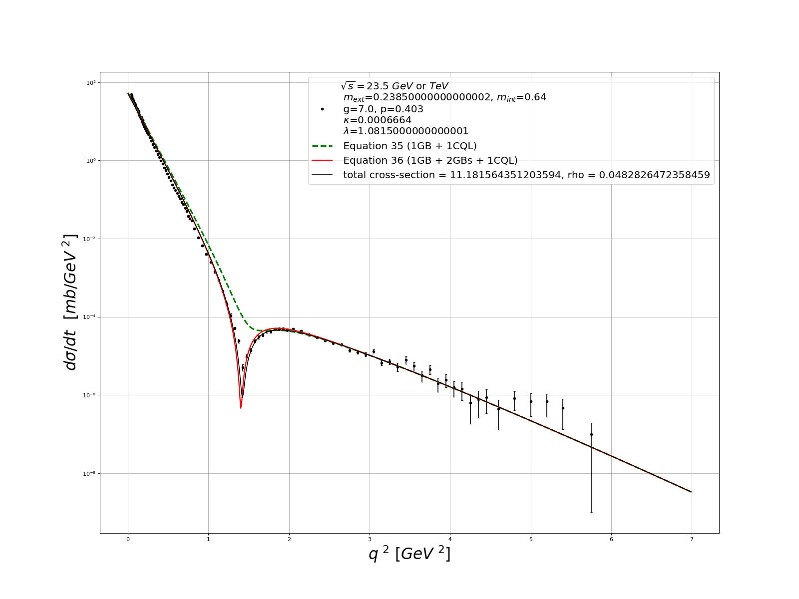
Figure 1: ISR = 23.5 GeV

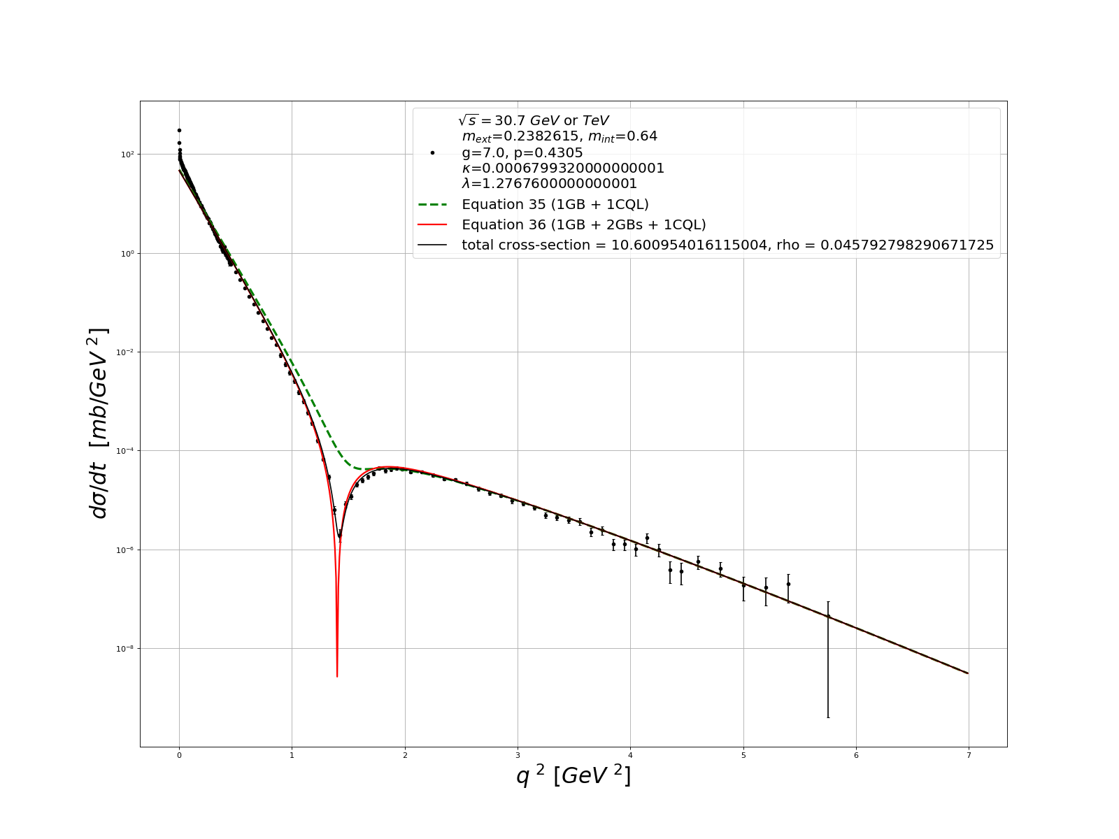
Figure 2: ISR = 30.7 GeV

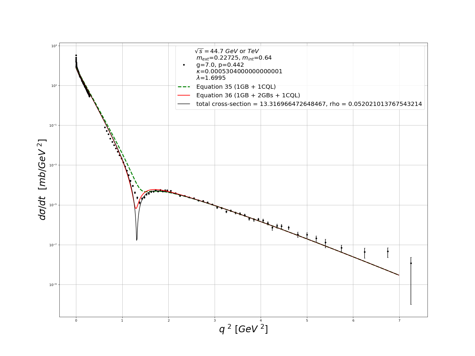
Figure 3: ISR = 44.7 GeV

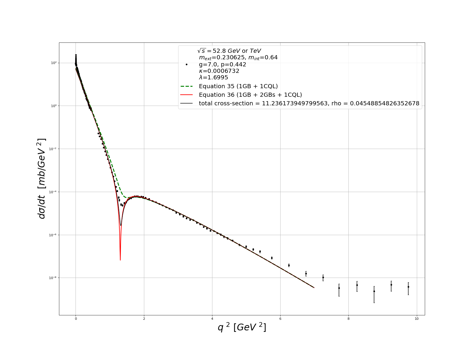
Figure 4: ISR = 52.8 GeV

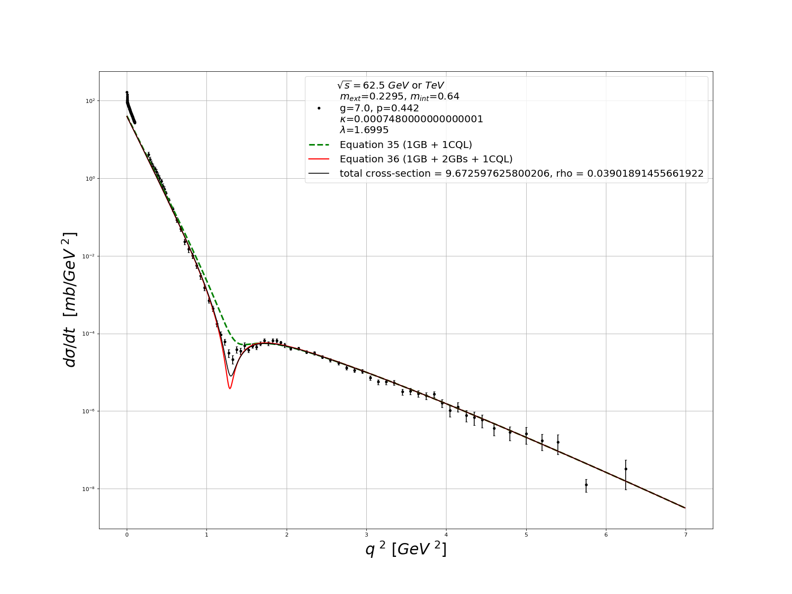
Figure 5: ISR = 62.5 GeV

Figure 6: ISR energies for elastic proton-proton scattering. Green dotted line for one Gluon Bundle and one Quark Loop Chain. Red solid line for One Gluon Bundle plus two Gluon Bundles and one Quark Loop Chain.

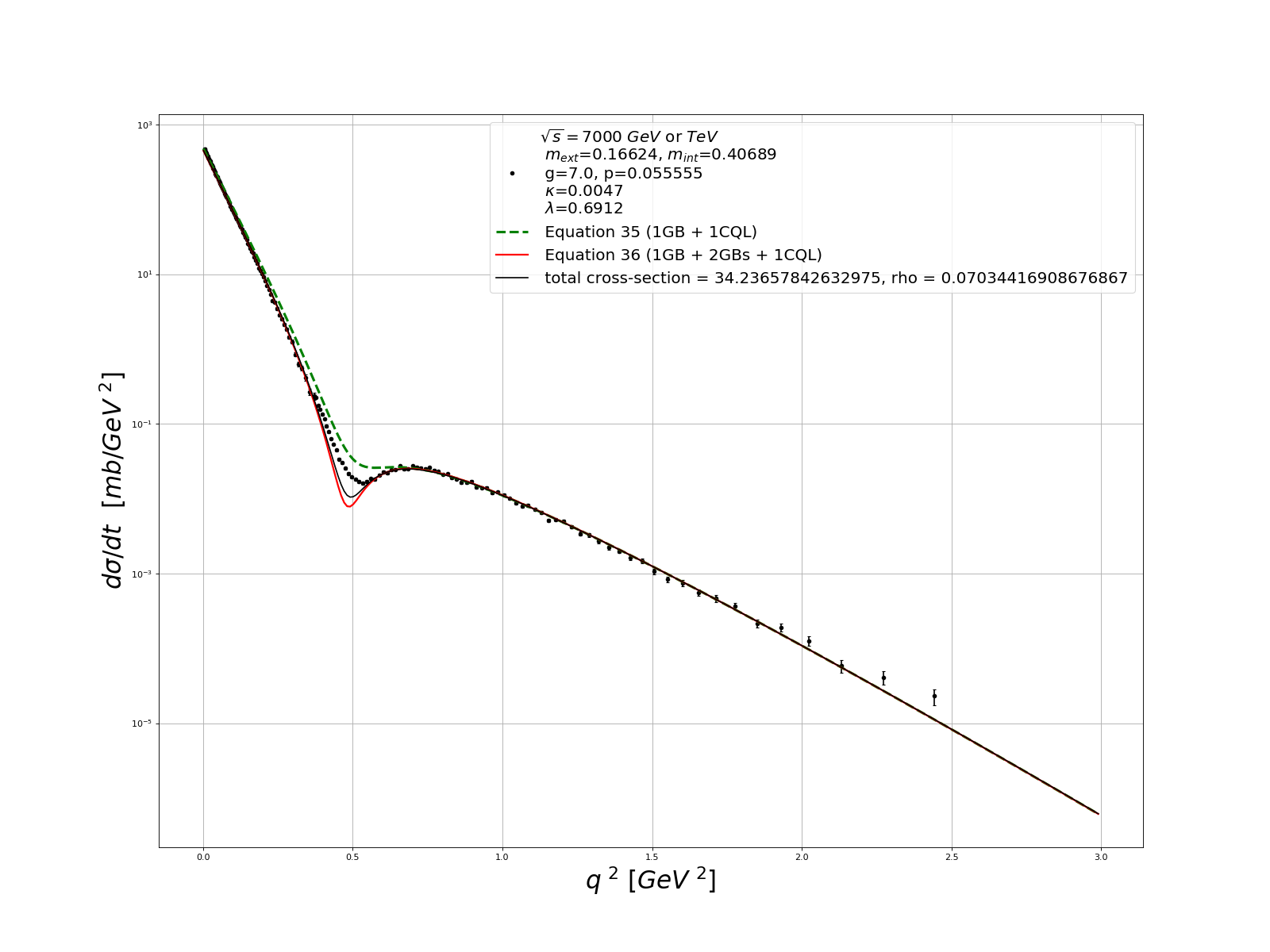
Figure 7: LHC-TOTEM = 7.0 TeV

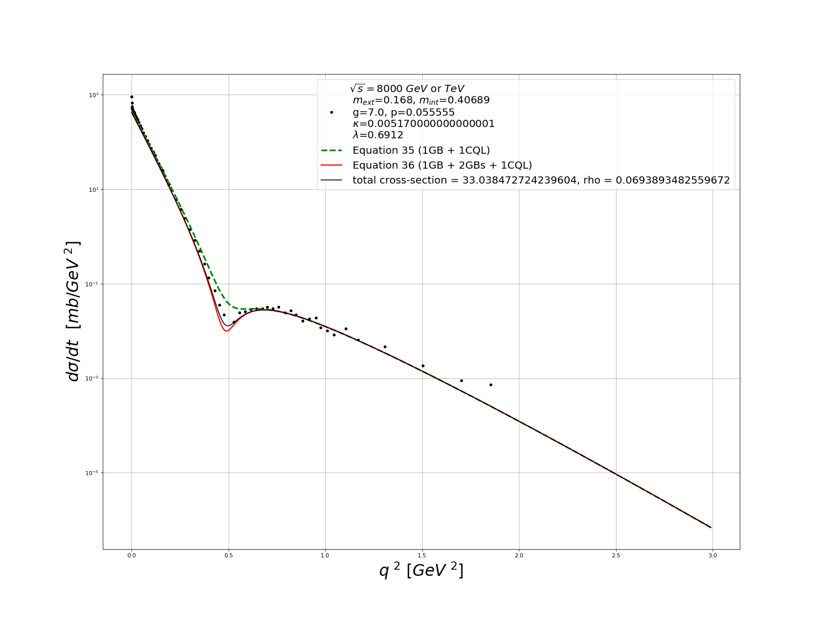
Figure 8: LHC-TOTEM = 8.0 TeV

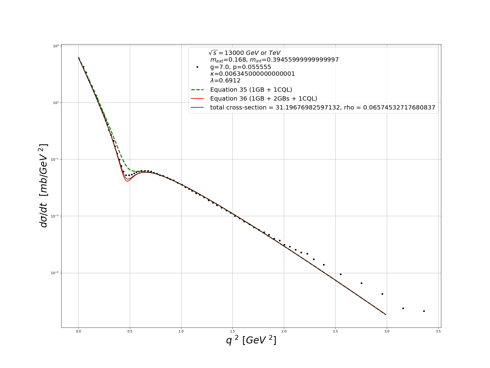
Figure 9: LHC-TOTEM = 13.0 TeV

Figure 10: LHC-TOTEM energies for elastic proton-proton scattering. Green dotted line for one Gluon Bundle and one Quark Loop Chain. Red solid line for One Gluon Bundle plus two Gluon Bundles and one Quark Loop Chain.

As shown in [1], [9], the choice for $\delta^{2}\ell=\kappa/\bar{m}$ results explicit $0$ for all graphs except Quark Loop Chain graphs.

The non-perturbative QCD scattering amplitude can thus be calculated as

$$T(s,\vec{q})=\frac{is}{2M^{2}}\int d^{2}be^{i\vec{q}\cdot\vec{b}}[1-e^{i\mathds{X}^{pp}(s,\vec{b})}]$$ (10)

Where $\mathds{X}^{pp}$ is the Eikonal of the proton-proton process where $e^{i\mathds{X}^{pp}}=e^{i\mathds{X}^{(GluonBundle)}}e^{i\mathds{X}^{(QuarkLoopChain)}}$

$$T(s,\vec{q})=\frac{is}{2M^{2}}\int d^{b}e^{i\vec{q}\cdot\vec{b}}[1-e^{\sqrt{i}g\delta^{2}_{q}\varphi(\vec{b})/2}e^{g^{2}\delta_{q}^{2}(\kappa/\bar{m}^{2})\Delta\bar{\varphi}/4}]$$ (11)

Expanding above we get for one gluon bundle plus one quark loop chain exchange:

$$T_{1}(s,\vec{q})=\frac{s}{2M^{2}}\frac{g}{2}(\frac{\lambda}{m})^{2}(\frac{m}{E})^{2p}[-\frac{1}{\sqrt{2}}e^{-q^{2}/4m^{2}}+i(\frac{1}{\sqrt{2}}e^{-q^{2}/4m^{2}}+\frac{g}{2}\kappa\frac{q^{2}}{\bar{m}^{2}}e^{-q^{2}/2\bar{m}^{2}})]$$ (12)

giving a differential cross section, (green dotted curve in figures)

$$\frac{d\sigma_{1}}{dt}(s,q^{2})=K\frac{27}{4\pi}\frac{g^{2}}{4}(\frac{\lambda}{4})^{4}(\frac{6m}{\sqrt{s}})^{4p}[\frac{1}{2}e^{-q^{2}/2m^{2}}+(\frac{1}{\sqrt{2}}e^{-q^{2}/4m^{2}}+\frac{g}{2}\kappa\frac{q^{2}}{\bar{m}^{2}}e^{-q^{2}/2\bar{m}^{2}})^{2}]$$ (13)

And for one gluon bundle plus two gluon bundles plus one quark loop chain exchange:

$$T_{2}(s,\vec{q})=\frac{s}{2M^{2}}\frac{g}{2}(\frac{\lambda}{m})^{2}(\frac{m}{E})^{2p}[(-\frac{1}{\sqrt{2}}e^{-q^{2}/4m^{2}}+\frac{1}{2}\frac{g}{2}\delta^{2}_{q}\frac{m^{2}}{2\pi}e^{-q^{2}/8m^{2}})+i(\frac{1}{\sqrt{2}}e^{-q^{2}/4m^{2}}+\frac{g}{2}\kappa\frac{q^{2}}{\bar{m}^{2}}e^{-q^{2}/2\bar{m}^{2}})]$$ (14)

with differential cross section (red solid line in figures)

$$\frac{d\sigma_{2}}{dt}(s,q^{2})=K\frac{27}{4\pi}\frac{g^{2}}{4}(\frac{\lambda}{m})^{4}(\frac{6m}{\sqrt{s}})^{4p}[(\frac{1}{2}e^{-q^{2}/2m^{2}}-\frac{g}{2}\frac{\lambda^{2}}{4\pi}(\frac{6m}{\sqrt{s}})^{2p}e^{-q^{2}/8m^{2}})^{2}+(\frac{1}{\sqrt{2}}e^{-q^{2}/4m^{2}}+\frac{g}{2}\kappa\frac{q^{2}}{\bar{m}^{2}}e^{-q^{2}/2\bar{m}^{2}})^{2}]$$ (15)

$K$ is conversion factor from mb to GeV at $0.44mbGeV^{-2}$. For the ISR data, we obtained parameters: g=7.0, p=0.13, $\lambda=0.5$, $\kappa=-6.810^{-4}$, $m=0.23GeV\approx 1.5m_{\pi}$, $\bar{m}=0.64GeV\approx 4.5m_{\pi}$.

For the LHC TOTEM data, we obtained $g=7.0$, $p=0.55$, $\lambda=0.72$, $\kappa=-4.210^{-3}$, $m=0.16GeV\approx m_{\pi}$, $\bar{m}=0.41GeV\approx 3m_{\pi}$.

References

References

• [1] H.M.Fried, Y. Gabellini, T. Grandou, Y.M. Sheu, P.H. Tsang. arXiv:1904.11083
• [2] H.M.Fried et al. Ann. Phys. 327, 2666-2690 (2012) DOI: 10.1016/j.aop.2012.07.008
• [3] Fried et al. Ann. Phys. 338, 2013 Volume 338, November 2013, Pages 107-122. DOI:10.1016/j.aop.2013.07.006
• [4] T. Grandou et al. Ann. Phys. 327 (2012), Mod. Phys. Lett. A, Vol.32(2017); arXiv:1706.02264
• [5] T. Grandou, P.H.Tsang, arXiv:1905:05666 . to be published
• [6] H.M.Fried, T.Grandou, Y.M.Sheu, Annals of Physics 344, 78-96 (2014), DOI:10.1016/j.aop.2014.02.015
• [7] H.M.Fried, P.H. Tsang arXiv:1502.04378.
• [8] T.Grandou, EPL (Europhysics Letters), Volume 107, Number 1. Article 11001. DOI:doi.org/10.1209/0295-5075/107/11001
• [9] H.M.Fried, Y.Gabellini, T.Grandou, Y.M.Sheu, P.H.Tsang., Annals of Physics Volume 359, August 2015, Pages 1-19. DOI: 10.1016/j.aop.2015.03.024
• [10] A.Casher(1979) Chiral symmetry breaking in quark confining theories. Phys Lett B 83:395–398.
• [11] S.J.Brodsky, R.Shrock. Proc. Nat. Acad. Sci. 108:45-50,2011. DOI: 10.1073/pnas.1010113107