Penalized regression via the restricted bridge estimator

Abstract.

This article is concerned with the Bridge Regression, which is a special family in penalized regression with penalty function $\sum_{j=1}^{p}|\beta_{j}|^{q}$ with $q>0$, in a linear model with linear restrictions. The proposed restricted bridge (RBRIDGE) estimator simultaneously estimates parameters and selects important variables when a prior information about parameters are available in either low dimensional or high dimensional case. Using local quadratic approximation, the penalty term can be approximated around a local initial values vector and the RBRIDGE estimator enjoys a closed-form expression which can be solved when $q>0$. Special cases of our proposal are the restricted LASSO ($q=1$), restricted RIDGE ($q=2$), and restricted Elastic Net ($1<q<2$) estimators. We provide some theoretical properties of the RBRIDGE estimator under for the low dimensional case, whereas the computational aspects are given for both low and high dimensional cases. An extensive Monte Carlo simulation study is conducted based on different prior pieces of information and the performance of the RBRIDGE estiamtor is compared with some competitive penalty estimators as well as the ORACLE. We also consider four real data examples analysis for comparison sake. The numerical results show that the suggested RBRIDGE estimator outperforms outstandingly when the prior is true or near exact.

^†Department of Econometrics

Inonu University, Turkey

E-mail address:b.yzb@hotmail.com

^‡Department of Statistics, Faculty of Mathematical Sciences

Shahrood University of Technology, Iran

E-mail address:m_arashi_stat@yahoo.com

^§Department of Mathematics and Computer Science

Cag University, Turkey

E-mail address :fikriakdeniz@gmail.com

1. Introduction

Under a linear regression setup, assume ${\bm{\beta}}=(\beta_{1},\ldots,\beta_{p})^{\top}$ is the vector of regression coefficients. Further, assume ${\bm{\beta}}$ is subjected to lie in a sub-space restriction with form

(1.1) $${\mathbf{R}}\bm{\beta}={\mathbf{r}},$$

where ${\mathbf{R}}$ is an $m\times p$ ($m<p$) matrix of constants and ${\mathbf{r}}$ is an $m$-vector of known prespecified constants. This restriction may be

(a):

a fact is known from theoretical or experimental considerations

(b):

a the hypothesis that may have to be tested, or

(c):

an artificially imposed condition to reduce or eliminate redundancy in the description of the model.

From a practical viewpoint, [Don, 1982] explained how accounting identities burden some exact restrictions on the endogenous variables in econometric models. [Xu and Yang, 2012] motivated the problem of estimating angles subject to summation. Recently [Kleyn et al., 2017] used a priori restriction present in labor and capital input in the estimation of Cobb-Douglass production function and inferred about the economic model using a preliminary testing approach.

Estimation with restriction (1.1) has been considered by many to decrease the mean squared error (MSE) of estimation and mean prediction error (MPE) in regression modeling. [Roozbeh, 2015] extended restricted ridge and the follow-up shrinkage strategies for the partially linear models and [Roozbeh, 2016] considered the robust extension of the latter work in restricted partially linear models. [Tuaç and Arslan, 2017] proposed a restricted LASSO in the restricted regression model, while [Norouzirad and Arashi, 2018] developed shrinkage estimators using LASSO and proposed a restricted LASSO to decrease the mean prediction error of estimation compared to the LASSO of [Tibshirani, 1996]. In a recent study, [Saleh et al., 2018] compared restricted estimators with LASSO and ridge in rank regression. For an extensive overview of restricted estimation in regression modeling and related shrinkage techniques, we refer to [Rao and Debasis, 2003], [Saleh, 2006], and [Radhakrishna Rao et al., 2008].

Our purpose here is sparse estimation with improving prediction accuracy, utilizing applying regularization techniques in regression modeling. However, the problem under study is different from the generalized LASSO (GLASSO) of [Tibshirani et al., 2011] and hence does not involve a penalty matrix. Simply we define restricted penalized estimator by imposing the sub-space restriction ${\mathbf{R}}\bm{\beta}={\mathbf{r}}$ to the estimation of the true parameter. We do not need any specific regularity assumption for the uniqueness as described by [Ali et al., 2019] as in the GLASSO. To be more specific, we use the solution of the bridge regularization technique as the “base estimator” and couple it with the specified restriction to obtain a closed-form restricted bridge estimator. As an instance, the restricted LASSO is a closed-form estimator based on the LASSO. Hence, our contribution has the following highlights:

Comparing to the existing methods (e.g., the GLASSO), the computational and temporal costs of our method are negligible.

It can be easily extended to other regularization techniques for which the local quadratic approximation (LQA) of [Fan and Li, 2001] can be applied for the penalty function, such as SCAD.

It improves the prediction accuracy of the base estimator and hence decrease the MPE.

It is consistent in estimation under the same regularity conditions as in the base estimator and is unique.

By the above description, the plan of this article is as follows. In Section 2, we describe the linear model along with bridge regularization technique. The restricted bridge is defined in Section 3, where we also derive its MSE and prove its consistency. Section 4 is devoted to two Monte Carlo simulation examples and the analysis of four real data examples are are given in Section 5 for performance analysis of the proposed restricted bridge estimator. We conclude our study in Section 6. Proofs of technical statements are given in the Appendix, to better focus on the computational part in the body of paper.

2. Statistical Model

Consider the following linear model

(2.1) $${\mathbb{Y}}={\mathbb{X}}_{n}\bm{\beta}+\bm{\varepsilon},$$

where ${\mathbb{Y}}=(Y_{1},\ldots,Y_{n})^{\top}$ is the vector of response variables, ${\mathbb{X}}_{n}=({\mathbf{x}}_{1},\ldots,{\mathbf{x}}_{n})^{\top}$ is the non-stochastic design matrix including $p$-dimensional covariates ${\mathbf{x}}_{i}\in\mathbb{R}^{p}$, and $\bm{\varepsilon}=(\varepsilon_{1},\ldots,\varepsilon_{n})^{\top}$ is the error term with $\mathbb{E}(\bm{\varepsilon})=\bm{0}$ and $\mathbb{E}(\bm{\varepsilon}\bm{\varepsilon}^{\top})=\bm{I}_{n}$. We also assume the observations $\{({\mathbf{x}}_{i},Y_{i})\}_{i=1}^{n}$ are centered, so there is no intercept in the model and the focus of this study is the estimation of $\bm{\beta}$.

The least squares (LS) estimator of ${\bm{\beta}}$ is given by $\tilde{{\bm{\beta}}}={\mathbf{C}}_{n}^{-1}{\mathbb{X}}_{n}^{\top}{\mathbb{Y}}$, with ${\mathbf{C}}_{n}={\mathbb{X}}_{n}^{\top}{\mathbb{X}}_{n}$. Under LS theory, as $n\to\infty$, we get $\sqrt{n}(\tilde{{\bm{\beta}}}-{\bm{\beta}})\overset{\mathcal{D}}{\to}N_{p}(\bm{0},{\mathbf{C}}^{-1})$, where we assumed the following regularity conditions hold

1. $\max_{1\leq i\leq n}{\mathbf{x}}_{i}^{\top}{\mathbf{C}}_{n}^{-1}{\mathbf{x}}_{i}\to 0$ as $n\to\infty$, where ${\mathbf{x}}_{i}^{\top}$ is the ith row of ${\mathbb{X}}_{n}$;

2. $n^{-1}{\mathbf{C}}_{n}\to{\mathbf{C}}$, where ${\mathbf{C}}$ is a finite positive definite (p.d.) matrix.

Despite simplicity of the LS estimator and that is the best linear unbiased estimator, its efficiency diminishes, in the MSE sense, in multicollinear and sparse situations. In these scenarios, regularization techniques are used to penalize large values of true regression parameters. As such we refer to the ridge and LASSO estimation methods, where $\textnormal{L}_{2}$ and $\textnormal{L}_{1}$ norms are used for the penalty term, respectively. [Frank and Friedman, 1993] introduced a class of regularization techniques called bridge, for which the penalty term allowed to very on $(0,\infty)$, i.e., $\textnormal{L}_{q}$ norm with $q>0$. This class includes the ridge and LASSO as special members. The bridge estimator can be obtained by solving the following optimization problem

$$\min_{{\bm{\beta}}\in\mathbb{R}^{p}}({\mathbb{Y}}-{\mathbb{X}}_{n}\bm{\beta})^{\top}({\mathbb{Y}}-{\mathbb{X}}_{n}\bm{\beta})\quad\textnormal{subject to}\quad\bm{1}_{p}^{\top}|\bm{\beta}|^{q}\leq t,\quad t\geq 0,$$

where $\bm{1}_{p}$ is a $p$-tuple of 1’s and $|\bm{\beta}|=(|\beta_{1}|,\ldots,|\beta_{p}|)^{\top}$. Consequently the bridge estimator is obtained by solving the dual form as

(2.2) $$\widehat{\bm{\beta}}_{n}=\mathop{\rm arg\,min}_{{\bm{\beta}}}\left\{\sum_{i=1}^{n}(Y_{i}-\bm{x}_{i}^{\top}\bm{\beta})^{2}+\lambda\sum_{j=1}^{p}|\beta_{j}|^{q}\right\},$$

where $\lambda$ is the tuning parameter and $q>0$.

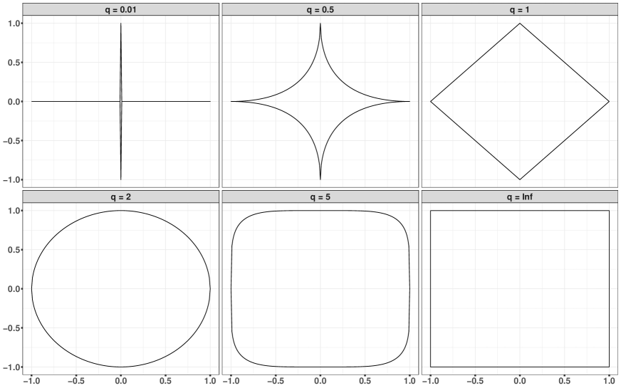
Figure 1. Constrained area of the bridge estimator with $t=1$

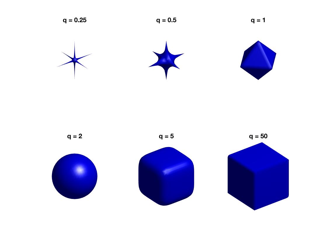
Figure 2. Shapes of different norms in 3D

Figure 1 shows the constrained area of the bridge estimator with $t=1$. Apparently, as $q$ increases the constrained area of penalty term widen, while for $q\to 0$, there is no penalty area and we get the LS solution, as we expect.

Using the local quadratic approximation (LQA) of [Fan and Li, 2001], the penalty term can be approximated around a local vector $\bm{\beta}^{o}$ and the bridge estimator has the following closed form

(2.3) $$\widehat{\bm{\beta}}_{n}=\left[{\mathbf{C}}_{n}+{\bm{\Sigma}}_{\lambda}(\widehat{\bm{\beta}}^{o})\right]^{-1}{\mathbb{X}}_{n}^{\top}{\mathbb{Y}},$$

where ${\bm{\Sigma}}_{\lambda}(\widehat{\bm{\beta}}^{o})=\frac{\lambda q}{2}\hbox{diag}\left(\left|\hat{\beta}_{1}^{o}\right|^{q-2},\dots,\left|\hat{\beta}_{p}^{o}\right|^{q-2}\right)$. See [Park and Yoon, 2011], for details.

3. Restricted Estimator

In order to couple the bridge estimator (termed as “base estimator” in the Introduction) with the specified restriction (1.1), we solve the following optimization problem

$$\min_{{\bm{\beta}}\in\mathbb{R}^{p}}({\mathbb{Y}}-{\mathbb{X}}_{n}\bm{\beta})^{\top}({\mathbb{Y}}-{\mathbb{X}}_{n}\bm{\beta})$$

s.t. $${\bm{\beta}}^{\top}\hbox{diag}\left(\left|\hat{\beta}_{1}^{o}\right|^{q-2},\dots,\left|\hat{\beta}_{p}^{o}\right|^{q-2}\right){\bm{\beta}}^{\top}\leq t,\;t>0\quad\mbox{and}\quad{\mathbf{R}}\bm{\beta}={\mathbf{r}},$$

where $(\beta^{o}_{1},\ldots,\beta^{0}_{p})$ are local points used in the LQA of [Fan and Li, 2001]. The solution of the above problem reveals the restricted bridge (BRIDGE) estimator in a closed form, as stated in the following result.

Theorem 3.1.

Assume linear model (2.1). Under the sub-space restriction (1.1), the RBRIDGE estimator is given by

(3.1) $$\widehat{\bm{\beta}}^{\rm R}_{n}=\widehat{\bm{\beta}}_{n}-({\mathbf{C}}+{\bm{\Sigma}}_{\lambda}(\widehat{\bm{\beta}}^{o}))^{-1}{\mathbf{R}}^{\top}\left[{\mathbf{R}}({\mathbf{C}}+{\bm{\Sigma}}_{\lambda}(\widehat{\bm{\beta}}^{o}))^{-1}{\mathbf{R}}^{\top}\right]^{-1}\left({\mathbf{R}}\widehat{\bm{\beta}}_{n}-{\mathbf{r}}\right).$$

Theorem 3.2.

Under the assumptions of Theorem 3.1 and linear restriction (1.1), we have

$$\mathrm{MSE}(\hat{\bm{\beta}}_{n}^{R})=\mathrm{tr}(\bm{M}[{\mathbf{S}}+{\bm{\Sigma}}_{\lambda}(\widehat{\bm{\beta}}^{o}){\bm{\beta}}^{\top}{\bm{\beta}}{\bm{\Sigma}}_{\lambda}(\widehat{\bm{\beta}}^{o})]\bm{M})$$

where ${\mathbf{S}}={\mathbf{C}}_{n}+{\bm{\Sigma}}_{\lambda}(\widehat{\bm{\beta}}^{o})$ and $\bm{M}={\mathbf{S}}^{-1}-{\mathbf{S}}^{-1}{\mathbf{R}}^{\top}({\mathbf{R}}{\mathbf{S}}^{-1}{\mathbf{R}}^{\top})^{-1}{\mathbf{R}}{\mathbf{S}}^{-1}$.

In the following result, we give the consistency property of the RBRIDGE estimator. For our purpose we assume $\lambda$ is dependent to $n$ and let $\lambda=\lambda_{n}$.

Theorem 3.3.

Under the assumptions of Theorem 3.2, the RBRIDGE estimator, with ${\mathbf{S}}$ replaced by ${\mathbf{S}}_{n}$, is consistent in estimation of ${\bm{\beta}}$ if $\lambda_{n}=o(n)$, where

$${\mathbf{S}}_{n}=\frac{1}{n}{\mathbf{C}}_{n}+\frac{1}{n}{\bm{\Sigma}}_{\lambda_{n}}(\widehat{\bm{\beta}}^{o}).$$

Since the RBRIDGE estimator has closed form, it is relatively simple to be computed. However, we use the LQA method in the body of optimization problem and hence we need to explain about the computation of RBRIDGE estimator. This task is taken care in the next section.

3.1. Computation of RBRIDGE estimator

Here, we briefly will outline the building block of our algorithm for computing the RBRIDGE estimator $\widehat{\bm{\beta}}_{n}^{\rm R}$.

With the aid of LQA, we derived a closed-form restricted bridge estimator (see Theorem 3.1). For a fast and high-performance computational algorithm, we specifically use the RcppArmadillo language of [Eddelbuettel and Sanderson, 2014]. For the selection of the tuning parameter $\lambda$, we use the following Cross-Validation (CV) method:

• Divide the data into $K$ roughly equal parts.

• For each $k=1,2,\dots,K$, compute the target estimator $\widehat{\bm{\beta}}_{n}^{-k}$, say using the rest of $K-1$ parts of the data.

• Compute the mean prediction error for the $k^{th}$ cycle by

  $$\mathrm{PE}_{k}(\lambda)=\frac{1}{n}\sum_{i\in k^{th}\mathrm{part}}(Y_{i}-\bm{x}_{i}^{\top}\widehat{\bm{\beta}}_{n}^{-k})^{2}$$

  .

• Finally, for many values of $\lambda$ calculate $\mathrm{CV_{\lambda}}=\frac{1}{K}\sum_{i=1}^{K}{\mathrm{PE}_{k}(\lambda)}$ and choose the $\lambda$ for which the smallest $\mathrm{CV_{\lambda}}$ is achieved.

In our computation, since the objective function (see the proof of Theorem 3.1) is convex, $\widehat{\bm{\beta}}_{n}^{\rm R}$ satisfies the necessary and sufficient Karush-Kuhn-Tucker (KKT) conditions, and hence we do not necessarily need them to be discussed here. Algorithm 1 below clarifies the steps for the whole computation procedure.

Algorithm 1 Details of the RBRIDGE algorithm

0:   Fix the values $q$ and $\lambda$.

0:   Set the initial value $\widehat{\bm{\beta}}^{o}$.

0:   Set the matrices ${\mathbf{R}}$ and ${\mathbf{r}}$ and compute

$$(\widehat{\bm{\beta}}^{\rm R}_{n})^{(t)}=(\widehat{\bm{\beta}}_{n})^{(t-1)}-({\mathbf{C}}+{\bm{\Sigma}}_{\lambda}(\widehat{\bm{\beta}}^{t-1}))^{-1}{\mathbf{R}}^{\top}\left[{\mathbf{R}}({\mathbf{C}}+{\bm{\Sigma}}_{\lambda}(\widehat{\bm{\beta}}^{(t-1)}))^{-1}{\mathbf{R}}^{\top}\right]^{-1}\left({\mathbf{R}}(\widehat{\bm{\beta}}_{n})^{(t-1)}-{\mathbf{r}}\right),$$

where $(\widehat{\bm{\beta}}_{n})^{(t-1)}=\left[{\mathbf{C}}_{n}+{\bm{\Sigma}}_{\lambda}(\widehat{\bm{\beta}}^{t-1})\right]^{-1}{\mathbb{X}}_{n}^{\top}{\mathbb{Y}}$ and ${\bm{\Sigma}}_{\lambda}(\widehat{\bm{\beta}}^{(t-1)})=\frac{\lambda q}{2}\hbox{diag}\left(\left|\hat{\beta}_{1}^{(t-1)}\right|^{q-2},\dots,\left|\hat{\beta}_{p}^{(t-1)}\right|^{q-2}\right)$ for $t=1,2,\dots$. The algorithm stops when $\left\|(\widehat{\bm{\beta}}^{\rm R}_{n})^{(t)}-(\widehat{\bm{\beta}}^{\rm R}_{n})^{(t-1)}\right\|<\eta$. During the iteration if $\left|\hat{\beta}_{j}^{(t-1)}\right|<\eta$, then we delete $j^{th}$ variable and exclude it from final model to make algorithm stable.

Remark 3.4.

In Algorithm 1, we used the ridge coefficients for Step 2 and $\eta=10^{-7}$.

Remark 3.5.

Algorithm 1 is just for the computation of RBRIDGE estimator. In our numerical studies, we will also consider the estimation of 2.3 following [Park and Yoon, 2011] for comparison sake.

4. Simulation

We generated response from the following model

$$y_{i}={\mathbf{x}}^{\top}_{i}{\bm{\beta}}+\sigma\epsilon_{i},\quad 1\leq i\leq n,$$

where ${\mathbf{x}}_{i}\in\mathbb{R}^{p}$ are zero mean multivariate normal random vectors with correlation matrix ${\bm{\Sigma}}=(\Sigma_{ij})$ with $\Sigma_{ij}=\rho^{|i-j|}$ and $\epsilon_{i}$ are standard normal. We consider $\sigma=1,3$ and $\rho=0.5,0.9$. There are two examples as follows:

• Following [Fan and Li, 2001, Tibshirani, 1996], we consider the true parameters as ${\bm{\beta}}=(3,1.5,0,0,2,0,0,0)^{\top}$ and generated data sets consisting of $n\in\{40,60\}$ observations. For the rest of simulation procedure we consider the following four scenarios about the specification of ${\mathbf{R}}$ and ${\mathbf{r}}$ matrices.

  Case 1- Let ${\mathbf{R}}=\left[1,1,0,0,1,0,0,0\right]$ and ${\mathbf{r}}=\left[6.5\right]$, that is, $\beta_{1}+\beta_{2}+\beta_{5}=6.5$.

  Case 2- Let ${\mathbf{R}}=\left[-1,1,0,0,1,0,0,0\right]$ and ${\mathbf{r}}=\left[0.5\right]$, that is, $\beta_{2}+\beta_{5}=\beta_{1}+0.5$.

  Case 3- We consider both cases (i) and (ii) simultaneously, that is, ${\mathbf{R}}=\left[\begin{matrix}1&1&0&0&1&0&0&0\\ -1&1&0&0&1&0&0&0\end{matrix}\right]$ and ${\mathbf{r}}=\begin{bmatrix}6.5\\ 0.5\\ \end{bmatrix}$.

  Case 4- Let ${\bm{\beta}}=\left({\bm{\beta}}_{1}^{\top},{\bm{\beta}}_{2}^{\top}\right)^{\top}$, where ${\bm{\beta}}_{1}$ presents the vector of non-zero variables of ${\bm{\beta}}$ while ${\bm{\beta}}_{2}$ presents zeros. As a special case of general form of null hypothesis ${\mathbf{R}}{\bm{\beta}}={\mathbf{r}}$, we consider ${\mathbf{R}}=\left[\begin{matrix}0&0&1&0&0&0&0&0\\ 0&0&0&1&0&0&0&0\\ 0&0&0&0&0&1&0&0\\ 0&0&0&0&0&0&1&0\\ 0&0&0&0&0&0&0&1\end{matrix}\right]$ and ${\mathbf{r}}=\begin{bmatrix}0\\ 0\\ 0\\ 0\\ 0\\ \end{bmatrix}$, that is, ${\bm{\beta}}_{2}=\begin{bmatrix}0\\ 0\\ 0\\ 0\\ 0\\ \end{bmatrix}$.

• This example is devoted to the situations where the number of co-variates is larger than the number of observations, which We only consider $n=50$ and $p=(100,200)$. The vector of true parameters is then taken as follows:

  $${\bm{\beta}}=\left(\underbrace{0,\dots,0}_{10},\underbrace{2,\dots,2}_{10},\underbrace{0,\dots,0}_{10},\underbrace{-2,\dots,-2}_{10},\underbrace{0,\dots,0}_{p-40}\right)^{\top}.$$

  Let again ${\bm{\beta}}=\left({\bm{\beta}}_{1}^{\top},{\bm{\beta}}_{2}^{\top}\right)^{\top}$, where ${\bm{\beta}}_{1}$ presents the vector of non-zero variables of ${\bm{\beta}}$ while ${\bm{\beta}}_{2}$ presents zeros. Hence, we consider the following four cases.

  Case 1- We consider an ${\mathbf{R}}=[{\mathbf{0}},{\mathbf{I}}]$ matrix where ${\mathbf{0}}$ and ${\mathbf{I}}$ are suitable sizes zero and identity matrices, respectively, such that ${\bm{\beta}}_{2}={\mathbf{r}}={\bf 1}_{p-20}^{\top}\cdot 0$.

  Case 2- Similar to the Case 1, except ${\mathbf{r}}={\bf 1}_{p-20}^{\top}\cdot 0.1$. In this case, we investigate violations of sub-model in Case 1.

  Case 3- Let ${\mathbf{R}}=[{\mathbf{I}},{\mathbf{0}}]$, where ${\mathbf{0}}$ and ${\mathbf{I}}$ are suitable sizes zero and identity matrices, respectively, such that ${\bm{\beta}}_{1}={\mathbf{r}}=({\bf 1}_{10}\cdot 2,{\bf 1}_{10}\cdot-2)^{\top}$.

  Case 4- This is similar to Case 3, except that ${\mathbf{r}}=({\bf 1}_{10}\cdot 2.1,{\bf 1}_{10}\cdot-2.1)^{\top}$. In this case, we investigate violations of sub-model in Case 3.

We also use the following criteria to asses the numerical performance:

• presents the median of the model error (ME) measure of an estimator, where ${\rm ME}=(\widehat{\bm{\beta}}-{\bm{\beta}})^{\top}\Sigma(\widehat{\bm{\beta}}-{\bm{\beta}})$.

• shows the average number of zero coefficients correctly estimated to be zero.

• shows the average number of nonzero coefficients incorrectly estimated to be zero.

• (Under fit) shows the proportion of excluding any significant variables.

• (Correct fit) presents the probability of selecting the exact subset model.

• (Over fit) shows the probability of including all three significant variables and some noise variables.

In our simulation study, we compare the performance of the RBRIDGE estimators with LASSO, RIDGE, Elastic Net (E-NET), SCAD, and ORACLE, which the latter is the ordinary least squares estimator of the true model, i.e., $y=\beta_{1}x_{1}+\beta_{2}x_{2}+\beta_{4}x_{4}$ for Example 1. For better specification the E-NET penalty term has form $\alpha\beta^{2}+(1-\alpha)|\beta|$. So, in our numerical analysis we consider LASSO($\alpha=1$), RIDGE($\alpha=0$) and E-NET($\alpha=0.2,0.4,0.6,0.8$ which gives minimum prediction error) using the glmnet package in R. For the SCAD we use the ncvreg package in R. Note that both the BRIDGE and RBRIDGE estimators are calculated using the rbridge package which will be appeared online soon. Also, a grid of values for $q$, from $0.25$ to $2$ with $0.25$ increment is taken, in addition to the one which gives the minimum measurement error.

Table 1. Simulation Results for Example 1

$n=40$, $\sigma=1$, $\rho=0.5$ $n=40$, $\sigma=1$, $\rho=0.9$ MME C IC U-fit C-fit O-fit MME C IC U-fit C-fit O-fit LASSO 0.154 2.768 0.000 0.000 0.118 0.882 0.461 2.888 0.000 0.000 0.102 0.898 RIDGE 0.296 0.000 0.000 0.000 0.000 1.000 1.175 0.000 0.000 0.000 0.000 1.000 E-NET 0.174 2.104 0.000 0.000 0.068 0.932 0.567 2.298 0.000 0.000 0.046 0.954 SCAD 0.082 4.444 0.000 0.000 0.756 0.244 0.554 3.970 0.172 0.170 0.420 0.410 ORACLE 0.064 5.000 0.000 0.000 1.000 0.000 0.156 5.000 0.000 0.000 1.000 0.000 BRIDGE 0.097 3.230 0.000 0.000 0.000 1.000 0.437 3.118 0.016 0.016 0.152 0.832 RBRIDGE¹ 0.160 2.358 0.000 0.000 0.268 0.732 0.551 1.706 0.010 0.010 0.156 0.834 RBRIDGE² 0.103 3.154 0.000 0.000 0.000 1.000 0.172 3.220 0.000 0.000 0.022 0.978 RBRIDGE³ 0.166 1.576 0.000 0.000 0.126 0.874 0.298 1.290 0.000 0.000 0.056 0.944 RBRIDGE⁴ 0.063 5.000 0.000 0.000 1.000 0.000 0.170 5.000 0.000 0.000 1.000 0.000 $n=40$, $\sigma=3$, $\rho=0.5$ $n=40$, $\sigma=3$, $\rho=0.9$ MME C IC U-fit C-fit O-fit MME C IC U-fit C-fit O-fit LASSO 1.374 2.796 0.034 0.034 0.122 0.844 3.615 2.950 0.416 0.386 0.082 0.532 RIDGE 1.783 0.000 0.000 0.000 0.000 1.000 3.251 0.000 0.000 0.000 0.000 1.000 E-NET 1.455 2.186 0.018 0.018 0.068 0.914 3.461 2.354 0.258 0.246 0.040 0.714 SCAD 1.770 3.352 0.172 0.166 0.166 0.668 7.120 3.622 1.110 0.804 0.020 0.176 ORACLE 0.579 5.000 0.000 0.000 1.000 0.000 1.407 5.000 0.000 0.000 1.000 0.000 BRIDGE 1.697 2.988 0.086 0.086 0.222 0.692 3.926 2.198 0.462 0.384 0.076 0.540 RBRIDGE¹ 0.682 1.162 0.022 0.022 0.116 0.862 1.297 1.500 0.182 0.180 0.076 0.744 RBRIDGE² 0.820 3.272 0.010 0.010 0.184 0.806 4.218 2.754 0.192 0.190 0.254 0.556 RBRIDGE³ 0.339 0.990 0.000 0.000 0.080 0.920 0.592 1.486 0.054 0.054 0.130 0.816 RBRIDGE⁴ 0.563 5.000 0.006 0.006 0.994 0.000 1.512 5.000 0.048 0.048 0.952 0.000 $n=60$, $\sigma=1$, $\rho=0.5$ $n=60$, $\sigma=1$, $\rho=0.9$ MME C IC U-fit C-fit O-fit MME C IC U-fit C-fit O-fit LASSO 0.094 2.696 0.000 0.000 0.102 0.898 0.267 2.916 0.000 0.000 0.086 0.914 RIDGE 0.211 0.000 0.000 0.000 0.000 1.000 1.046 0.000 0.000 0.000 0.000 1.000 E-NET 0.104 2.146 0.000 0.000 0.056 0.944 0.328 2.432 0.000 0.000 0.050 0.950 SCAD 0.050 4.480 0.000 0.000 0.770 0.230 0.178 4.270 0.050 0.050 0.634 0.316 ORACLE 0.039 5.000 0.000 0.000 1.000 0.000 0.098 5.000 0.000 0.000 1.000 0.000 BRIDGE 0.057 3.114 0.000 0.000 0.000 1.000 0.188 3.220 0.004 0.004 0.070 0.926 RBRIDGE¹ 0.108 2.684 0.000 0.000 0.338 0.662 0.353 1.842 0.002 0.002 0.172 0.826 RBRIDGE² 0.070 3.008 0.000 0.000 0.000 1.000 0.092 3.190 0.000 0.000 0.014 0.986 RBRIDGE³ 0.122 1.626 0.000 0.000 0.140 0.860 0.203 1.434 0.000 0.000 0.088 0.912 RBRIDGE⁴ 0.040 5.000 0.000 0.000 1.000 0.000 0.103 5.000 0.000 0.000 1.000 0.000 $n=60$, $\sigma=3$, $\rho=0.5$ $n=60$, $\sigma=3$, $\rho=0.9$ MME C IC U-fit C-fit O-fit MME C IC U-fit C-fit O-fit LASSO 0.851 2.696 0.004 0.004 0.102 0.894 2.266 2.864 0.216 0.208 0.076 0.716 RIDGE 1.095 0.000 0.000 0.000 0.000 1.000 2.497 0.000 0.000 0.000 0.000 1.000 E-NET 0.907 2.246 0.002 0.002 0.058 0.940 2.356 2.346 0.142 0.136 0.032 0.832 SCAD 0.918 3.478 0.068 0.068 0.246 0.686 3.822 3.676 0.838 0.686 0.062 0.252 ORACLE 0.355 5.000 0.000 0.000 1.000 0.000 0.883 5.000 0.000 0.000 1.000 0.000 BRIDGE 0.844 3.110 0.030 0.030 0.146 0.824 2.744 2.240 0.304 0.272 0.132 0.596 RBRIDGE¹ 0.562 1.358 0.004 0.004 0.124 0.872 0.901 1.254 0.124 0.124 0.076 0.800 RBRIDGE² 0.466 3.182 0.000 0.000 0.056 0.944 2.495 2.860 0.098 0.098 0.244 0.658 RBRIDGE³ 0.265 1.004 0.000 0.000 0.056 0.944 0.380 1.366 0.020 0.020 0.106 0.874 RBRIDGE⁴ 0.351 5.000 0.000 0.000 1.000 0.000 0.965 5.000 0.010 0.010 0.990 0.000

¹the restrictions in case 1, ²the restrictions in case 2, ³the restrictions in case 3, ⁴the restrictions in case 4.

In Table 1, we report the the result obtained from the simulation study of Example 1 and briefly summarize as follows: if the sample size is small, the noise level is low and the the effect of multicollinearity is moderate, the SCAD performs well compared to the LASSO, RIDGE and E-NET and it reduces both ME and model complexity (MC). If the noise level is high with same the $n$ and $\rho$, the LASSO becomes better which is consistent with the results of [Fan and Li, 2001]. Apart from their results, we notice that SCAD loses its efficiency in terms of both the ME and MC as $\rho$ gets large. RIDGE may only reduce ME and does not reduce MC since it does not shrink coefficients to zero. The E-NET has advantage compared to the RIDGE since it shrinks coefficients to zero even if it has larger ME compared to the RIDGE. With this analysis in hand, we now concentrate on performance evaluation of the proposed $L_{q}$-type estimation. We first note that the performance of the RBRIDGE⁴ is mostly close to the ORACLE which means it reduces both the ME and MC. When the noise level is low, the RBRIDGE², which is the Case 2 of restrictions, has better performance compared to Cases 1 and 3. On the other hand, as the noise level gets larger, the RBRIDGE³ that is estimated based on the combination of both the restrictions in Cases 1 & 2 reduces the ME more than that of the RBRIDGE¹ and RBRIDGE². Also, the MMEs of the proposed estimators become generally smaller as $n$ increases.

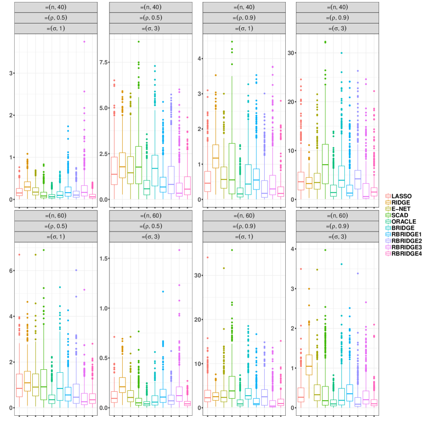
Figure 3. Boxplots of the MEs for Example 1

Among all, the RBRIDGE⁴ is preferred with respect to the others measures, C, IC, U-fit, C-fit, and O-fit.

Table 2. Simulation Results for Example 2

$p=100$, $\sigma=1$, $\rho=0.5$ $p=100$, $\sigma=1$, $\rho=0.9$ MME C IC U-fit C-fit O-fit MME C IC U-fit C-fit O-fit LASSO 3.091 63.74 0.08 0.06 0.0 0.94 1.520 74.46 0.12 0.12 0.00 0.88 RIDGE 114.298 0.00 0.00 0.00 0.0 1.00 127.445 0.00 0.00 0.00 0.00 1.00 E-NET 3.537 60.42 0.04 0.04 0.0 0.96 0.994 72.66 0.00 0.00 0.00 1.00 SCAD 61.240 73.34 8.66 1.00 0.0 0.00 24.683 77.20 14.00 1.00 0.00 0.00 ORACLE 0.527 80.00 0.00 0.00 1.0 0.00 0.663 80.00 0.00 0.00 1.00 0.00 BRIDGE 1.106 70.70 0.08 0.04 0.1 0.86 1.554 33.56 0.42 0.18 0.00 0.82 RBRIDGE¹ 0.497 80.00 0.00 0.00 1.0 0.00 0.317 80.00 0.00 0.00 1.00 0.00 RBRIDGE² 4.110 0.00 0.00 0.00 0.0 1.00 11.480 0.00 0.40 0.06 0.00 0.94 RBRIDGE³ 0.094 47.76 0.00 0.00 0.0 1.00 0.107 43.12 0.00 0.00 0.00 1.00 RBRIDGE⁴ 0.840 46.94 0.00 0.00 0.0 1.00 1.221 46.08 0.00 0.00 0.00 1.00 $p=100$, $\sigma=3$, $\rho=0.5$ $p=100$, $\sigma=3$, $\rho=0.9$ MME C IC U-fit C-fit O-fit MME C IC U-fit C-fit O-fit LASSO 21.047 63.16 1.44 0.66 0.0 0.34 7.473 71.22 3.18 0.98 0.00 0.02 RIDGE 113.484 0.00 0.00 0.00 0.0 1.00 127.367 0.00 0.00 0.00 0.00 1.00 E-NET 19.890 57.24 0.76 0.44 0.0 0.56 5.884 69.00 1.10 0.56 0.00 0.44 SCAD 74.389 74.30 9.70 1.00 0.0 0.00 29.122 77.12 14.20 1.00 0.00 0.00 ORACLE 4.744 80.00 0.00 0.00 1.0 0.00 5.971 80.00 0.00 0.00 1.00 0.00 BRIDGE 24.677 28.18 1.52 0.40 0.0 0.60 7.863 23.84 2.00 0.32 0.00 0.68 RBRIDGE¹ 3.821 80.00 0.00 0.00 1.0 0.00 1.694 80.00 0.26 0.04 0.96 0.00 RBRIDGE² 6.817 0.00 0.00 0.00 0.0 1.00 12.274 0.00 0.74 0.08 0.00 0.92 RBRIDGE³ 0.506 35.00 0.00 0.00 0.0 1.00 0.531 46.00 0.00 0.00 0.00 1.00 RBRIDGE⁴ 1.286 46.56 0.00 0.00 0.0 1.00 1.969 38.24 0.00 0.00 0.00 1.00 $p=200$, $\sigma=1$, $\rho=0.5$ $p=200$, $\sigma=1$, $\rho=0.9$ MME C IC U-fit C-fit O-fit MME C IC U-fit C-fit O-fit LASSO 43.233 162.98 4.00 0.86 0.0 0.14 2.885 171.66 0.64 0.42 0.00 0.58 RIDGE 139.543 0.00 0.00 0.00 0.0 1.00 167.377 0.00 0.00 0.00 0.00 1.00 E-NET 40.517 155.14 2.46 0.76 0.0 0.24 2.061 168.50 0.08 0.08 0.00 0.92 SCAD 117.997 175.56 12.10 1.00 0.0 0.00 40.314 175.20 14.98 1.00 0.00 0.00 ORACLE 0.959 180.00 0.00 0.00 1.0 0.00 0.974 180.00 0.00 0.00 1.00 0.00 BRIDGE 46.456 121.66 3.34 0.58 0.0 0.42 3.577 157.72 1.40 0.58 0.00 0.42 RBRIDGE¹ 0.936 180.00 0.00 0.00 1.0 0.00 0.398 180.00 0.00 0.00 1.00 0.00 RBRIDGE² 9.470 0.00 0.00 0.00 0.0 1.00 33.882 0.00 0.46 0.04 0.00 0.96 RBRIDGE³ 0.311 102.98 0.00 0.00 0.0 1.00 0.140 93.24 0.00 0.00 0.00 1.00 RBRIDGE⁴ 1.294 66.74 0.00 0.00 0.0 1.00 1.770 114.22 0.00 0.00 0.00 1.00 $p=200$, $\sigma=3$, $\rho=0.5$ $p=200$, $\sigma=3$, $\rho=0.9$ MME C IC U-fit C-fit O-fit MME C IC U-fit C-fit O-fit LASSO 56.255 163.62 5.76 0.96 0.0 0.04 13.064 167.04 4.74 1.00 0.00 0.00 RIDGE 139.681 0.00 0.00 0.00 0.0 1.00 167.472 0.00 0.00 0.00 0.00 1.00 E-NET 53.906 152.80 3.62 0.90 0.0 0.10 11.059 163.66 1.84 0.70 0.00 0.30 SCAD 118.643 176.00 12.78 1.00 0.0 0.00 43.988 174.40 15.36 1.00 0.00 0.00 ORACLE 8.633 180.00 0.00 0.00 1.0 0.00 8.769 180.00 0.00 0.00 1.00 0.00 BRIDGE 62.173 89.22 3.14 0.52 0.0 0.48 15.952 117.10 5.38 0.66 0.00 0.34 RBRIDGE¹ 5.592 180.00 0.00 0.00 1.0 0.00 1.987 180.00 0.28 0.04 0.96 0.00 RBRIDGE² 13.364 0.00 0.12 0.02 0.0 0.98 35.756 0.00 1.46 0.14 0.00 0.86 RBRIDGE³ 2.503 49.80 0.00 0.00 0.0 1.00 0.433 73.88 0.00 0.00 0.00 1.00 RBRIDGE⁴ 3.202 50.12 0.00 0.00 0.0 1.00 2.674 66.62 0.00 0.00 0.00 1.00

¹the restrictions in case 1, ²the restrictions in case 2, ³the restrictions in case 3, ⁴the restrictions in case 4.

As the noise level increases its performance violates, however, it is still the best amongst. On the other hand, the O-fit of other RBRIDGE estimators are higher than the rest. However, the O-fit decreases as noise level increases. Eventually, as the level of multicollinearity increases the C-fit measure of the proposed estimators decreases, which is compatible with other penalty estimators. In the Figure 3, we plot MEs, which the figures outputs agree with the reported analyses.

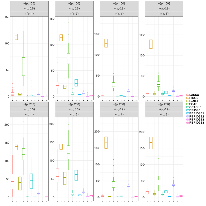
Figure 4. Boxplots of the MEs for Example 2.

Similar to Table 1, Table 2 provides the summary for the high dimensional case in which the number of co-variates exceeds the number of samples. Obviously both ME and MC measures increase in this case, however, as the sample size increases the values decrease that show consistency in estimation. As the noise level increases the performance of the proposed RBRIDGE estimators is as good as the oracle, however, the other penalty estimators perform poorly. To be more specific, it is clearly seen that both the RIDGE and SCAD perform very poor in terms of the ME and MC in most cases. This gets much worse if $p$ increases. In terms of estimation accuracy the RBRIDGE estimators perform closely to the oracle estimator, whereas our proposed approach gives the smallest MME, and consistently outperforms other penalty estimators. In terms of variable selection we observe that the well-known penalty estimators does not lead to a sparse model with restriction, whereas, the RBRIDGE estimators successfully select all covariates with nonzero coefficients, but it is obvious that the proposed RBRIDGE² has slightly strange sparsity rate (i.e., zero Cs) than the other RBRIDGE estimators. Figure 4, we plot MEs; again confirm the performance analysis outlined in above.

5. Real Data Analyses

We exhaustively consider four real data examples which cover both low dimensional and high dimensional cases. Each data set is freely available online and can be downloaded from the given references. In all applications, we analyze the performance of the respective approaches in the simulation. Before we start analyzing, the response variable is centered and the predictors are standardized. Hence, a constant term is not counted as a parameter. To asses the prediction accuracy of the listed estimators, we randomly split the data into two equal part of observations, the first part is the training set and the other part is for test set. Models are fitted on the training set only. We consider the following measure to asses the performance of the estimators.

(5.1) $$\rm MSE_{y}=\left\|{\mathbf{y}}_{test}-{\mathbb{X}}_{test}\widehat{\bm{\beta}}\right\|^{2}$$

We also consider the following measure in the case where a prior information ${\bm{\beta}}_{0i}$, $i=1,2$, is available.

(5.2) $$\rm MSE_{{\bm{\beta}}_{0i}}=\left\|{\bm{\beta}}_{0i}-\widehat{\bm{\beta}}\right\|^{2},i=1,2.$$

For clarity, here $i$ takes two values since we consider two sets of prior information (restrictions) in our numerical analyses.

This process is repeated $500$ times if $n>p$, otherwise $100$, and the median values are reported. For the ease of comparison, we calculate the $\rm RMSE=\frac{\rm MSE}{\min\rm MSE}$; values larger than $1$ show the estimator performs worse compared to the one that has the minimum MSE.

5.1. Air Pollution and Mortality Data

Air pollution has an impact on health and leads to disease or hospitalization if someone has been exposed to excessive air pollution for a long time. Everyone may be exposed to air pollution.

Variables	Descriptions
Mortality(Response)	Total age-adjusted mortality from
	all causes (Annual deaths per 100,000 people)
Precip	Mean annual precipitation (inches)
Humidity	Percent relative humidity (annual average at 1:00pm)
JanTemp	Mean January temperature (degrees F)
JulyTemp	Mean July temperature (degrees F)
Over65	Percentage of the population aged 65 years or over
House	Population per household
Educ	Median number of school years completed for persons 25 years or older
Sound	Percentage of the housing that is sound with all facilities
Density	Population density (in persons per square mile of urbanized area)
NonWhite	Percentage of population that is nonwhite
WhiteCol	Percentage of employment in white collar occupations
Poor	Percentage of households with annual income under $3,000 in 1960
HC	Pollution potential of hydrocarbons
NOX	Pollution potential of oxides of nitrogen
SO2	Pollution potential of sulfur dioxide

Table 3. Description of the Air Pollution and Mortality Data variables

Hence, it is worth to investigate what kinds of variable effects mortality. In this example, we use the well-known Air Pollution and Mortality Data which is originally analyzed by [McDonald and Schwing, 1973] and was also analyzed by [Soofi, 1990, Smucler and Yohai, 2017, Yüzbaşı et al., 2019]. The data are freely available at http://lib.stat.cmu.edu/datasets/pollution. This data consists of 60 sets observations of metropolitan statistical areas in the United States in 1960 on 16 variables, where the description of the variables is provided in Table 3.

To estimate the RBRIDGE, we need to know a piece of prior information about the real data set. This can be adopted from the previous results, e.g., [McDonald and Schwing, 1973, Yüzbaşı et al., 2019] or an expert’s opinion can be taken. However, we used the stepwise regressions here, making use of the functions ols_step_forward_p and ols_step_backward_p in olsrr package which is recently realized in R. Hence, we have two prior information that are reported in Table 4. According to this table, the “Stepwise Forward Method” finds that seven variables are significantly important while the other method finds that nine variables are significantly important.

Table 4. True parameters based on the Stepwise regression

		Stepwise Forward Method	Stepwise Backward Method
	Variables	${\bm{\beta}}_{01}$	${\bm{\beta}}_{02}$
$\beta_{1}$	Precip	16.460	18.536
$\beta_{2}$	Humidity	–	–
$\beta_{3}$	JanTemp	-19.256	-23.005
$\beta_{4}$	JulyTemp	-10.956	-15.812
$\beta_{5}$	Over65	–	-15.994
$\beta_{6}$	House	-8.387	-18.582
$\beta_{7}$	Educ	-14.338	-19.796
$\beta_{8}$	Sound	–	–
$\beta_{9}$	Density	–	–
$\beta_{10}$	NonWhite	46.530	41.590
$\beta_{11}$	WhiteCol	–	–
$\beta_{12}$	Poor	–	–
$\beta_{13}$	HC	–	-84.819
$\beta_{14}$	NOX	–	86.698
$\beta_{15}$	SO2	14.284	–

In the light of the prior information in Table 4, the restrictions based on ${\bm{\beta}}_{01}$ and ${\bm{\beta}}_{02}$ can be respectively expressed as follows:

(5.3) $${\mathbf{R}}_{1}=\begin{bmatrix}\begin{tabular}[]{rrrrrrrrrrrrrrrr}0&1&0&0&0&0&0&0&0&0&0&0&0&0&0\\ 0&0&0&0&1&0&0&0&0&0&0&0&0&0&0\\ 0&0&0&0&0&0&0&1&0&0&0&0&0&0&0\\ 0&0&0&0&0&0&0&0&1&0&0&0&0&0&0\\ 0&0&0&0&0&0&0&0&0&0&1&0&0&0&0\\ 0&0&0&0&0&0&0&0&0&0&0&1&0&0&0\\ 0&0&0&0&0&0&0&0&0&0&0&0&1&0&0\\ 0&0&0&0&0&0&0&0&0&0&0&0&0&1&0\end{tabular}\end{bmatrix}, {\mathbf{r}}_{1}=\begin{bmatrix}0\\ 0\\ 0\\ 0\\ 0\\ 0\\ 0\\ 0\\ \end{bmatrix},$$

that is, $\beta_{i}=0$, $i=2,5,8,9,11,12,13,14$ and

(5.4) $${\mathbf{R}}_{2}=\begin{bmatrix}\begin{tabular}[]{rrrrrrrrrrrrrrrr}0&1&0&0&0&0&0&0&0&0&0&0&0&0&0\\ 0&0&0&0&0&0&0&1&0&0&0&0&0&0&0\\ 0&0&0&0&0&0&0&0&1&0&0&0&0&0&0\\ 0&0&0&0&0&0&0&0&0&0&1&0&0&0&0\\ 0&0&0&0&0&0&0&0&0&0&0&1&0&0&0\\ 0&0&0&0&0&0&0&0&0&0&0&0&0&0&1\end{tabular}\end{bmatrix}, {\mathbf{r}}_{2}=\begin{bmatrix}0\\ 0\\ 0\\ 0\\ 0\\ 0\\ \end{bmatrix},$$

that is, $\beta_{i}=0$, $i=2,8,9,11,12,15$. The results of analysis are reported in Table 5. We expect that the RBRIDGE estimators based on the prior information perform well compared to the other penalty estimators in terms of the measure of ${\rm MSE_{\beta_{0}}}$. The RBRIDGE¹ has an improvement $3.375$ times more than the BRIDGE and is at least $2.75$ times better than the others since it is estimated by using the restrictions based on the true parameter ${\bm{\beta}}_{01}$. By looking at $\rm MSE_{\beta_{02}}$, the RBRIDGE² has an improvement $1.759$ times more than the BRIDGE and is at least $1.67$ times better than the others since it is constructed based on ${\bm{\beta}}_{02}$. On the other hand, it can be also seen that the RBRIDGE¹ outshines the others since it has the lowest prediction error, which is shown at ${\rm MSE_{y}}$, even better than the RBRIDGE². In the last column of Table 5 we also report the median of the number selected variables throughout replications.

Table 5. Performance analysis of the estimators for the Air Pollution and Mortality Data

	$\rm MSE_{y}$	$\rm RMSE_{y}$	$\rm MSE_{\beta_{01}}$	$\rm RMSE_{\beta_{01}}$	$\rm MSE_{\beta_{02}}$	$\rm RMSE_{\beta_{02}}$	# variable
LASSO	46745.635	1.213	1038.526	2.756	16503.929	1.747	8
RIDGE	47758.527	1.239	1414.969	3.755	15814.735	1.674	15
E-NET	46344.879	1.203	1118.269	2.968	16499.733	1.746	9
SCAD	53071.400	1.377	1169.844	3.104	16595.772	1.756	6
BRIDGE	49280.423	1.279	1271.908	3.375	16621.214	1.759	7
RBRIDGE1	38534.576	1.000	376.837	1.000	15846.628	1.677	7
RBRIDGE2	46518.768	1.207	4447.006	11.801	9448.353	1.000	9

¹the restrictions based on Stepwise Forward, ²the restrictions based on Stepwise Backward

In Table 6, we report the estimates along with the tuning parameters used in the proposed penalty estimators to better understanding of methods.

Table 6. Estimated coefficients of Air Pollution and Mortality Data

LASSO RIDGE E-NET SCAD BRIDGE RBRIDGE¹ RBRIDGE² $\lambda=2.023$ $\lambda=8.358$ $\lambda=2.168$ $\lambda=2.272$ $\lambda=373.815$ $\lambda=0.318$ $\lambda=15.883$ $\alpha=0.850$ $q=0.800$ $q=0.050$ $q=1.250$ $\widehat{\beta}_{1}$ Precip 15.037 16.168 15.198 16.869 15.805 16.460 16.498 $\widehat{\beta}_{2}$ Humidity – 1.894 0.047 – – – – $\widehat{\beta}_{3}$ JanTemp -12.101 -12.028 -12.077 -18.120 -13.551 -19.256 -22.965 $\widehat{\beta}_{4}$ JulyTemp -6.000 -6.815 -6.257 -11.029 -7.013 -10.956 -13.347 $\widehat{\beta}_{5}$ Over65 – -4.123 – – – – -9.866 $\widehat{\beta}_{6}$ House – -2.190 – -6.036 – -8.387 -14.834 $\widehat{\beta}_{7}$ Educ -8.786 -7.303 -8.498 -13.269 -10.156 -14.338 -19.485 $\widehat{\beta}_{8}$ Sound -2.658 -5.964 -3.010 – – – – $\widehat{\beta}_{9}$ Density 5.281 7.527 5.510 1.606 4.626 – – $\widehat{\beta}_{10}$ NonWhite 35.548 29.234 35.519 45.147 38.156 46.530 44.580 $\widehat{\beta}_{11}$ WhiteCol -0.066 -2.243 -0.281 – – – – $\widehat{\beta}_{12}$ Poor – 2.203 – – – – – $\widehat{\beta}_{13}$ HC – -3.583 – – – – -47.870 $\widehat{\beta}_{14}$ NOX – 3.276 – – – – 50.958 $\widehat{\beta}_{15}$ SO2 14.471 15.255 14.574 14.231 14.090 14.284 –

¹the restrictions based on Stepwise Forward, ²the restrictions based on Stepwise Backward

Finally, the 3D plot of the cross validation errors (CVE) of the RBRIDGE estimator versus $q$ and $log(\lambda)$ is plotted.

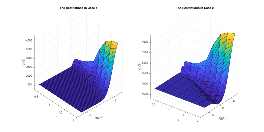
Figure 5. The 3D plot of the CVE of the RBRIDGE estimator versus $q$ and $log(\lambda)$ for Air Pollution and Mortality Data under the restrictions Stepwise Forward and Backward, respectively.

5.2. Gorman–Toman Data

A Ten-Factor data set first described by [Gorman and Toman, 1966] and used by several authors. c.f., [Hocking and Leslie, 1967, Hoerl and Kennard, 1970, Gunst et al., 1976, Özkale, 2014]. One may freely obtain this data from the ridge package in R, [Cule, 2019]. The data set has $36$ observations, which shows one day of operation of a petroleum refining unit, on $10$ independent variables and one dependent variable. We consider three different scenarios on the restrictions following the explanations of [Özkale, 2014].

• [Gunst et al., 1976] conducted that there exists multicollinearity among the variables of $X_{1}.X_{5}$ and $X_{6}$. [Özkale, 2014] identified the restriction $\beta_{1}+\beta_{5}+\beta_{6}=0$. This restriction can be expressed as ${\mathbf{R}}_{1}=\begin{bmatrix}1&0&0&0&1&1&0&0&0&0\end{bmatrix}$ and ${\mathbf{r}}_{1}=0$.

• Based on the $\rm C_{p}$ statistic, [Hoerl and Kennard, 1970] demonstrated that the first, fourth, ninth and tenth explanatory variables may be ignored since they are not significantly important. Hence, we have the restriction $\beta_{1}=0$, $\beta_{4}=0$, $\beta_{9}=0$ and $\beta_{10}=0$ which yields ${\mathbf{R}}_{2}=\begin{bmatrix}\begin{tabular}[]{rrrrrrrrrr}1&0&0&0&0&0&0&0&0&0\\ 0&0&0&1&0&0&0&0&0&0\\ 0&0&0&0&0&0&0&0&1&0\\ 0&0&0&0&0&0&0&0&0&1\\ \end{tabular}\end{bmatrix}$ and ${\mathbf{r}}_{2}=\begin{bmatrix}0\\ 0\\ 0\\ 0\\ \end{bmatrix}$.

• Finally, following [Hocking and Leslie, 1967], the elements of the restriction are given by ${\mathbf{R}}_{3}=\begin{bmatrix}\begin{tabular}[]{rrrrrrrrrr}0&0&0&0&1&0&0&0&0&0\\ 0&0&0&0&0&1&0&0&0&0\\ 0&0&0&0&0&0&1&0&0&0\\ 0&0&0&0&0&0&0&1&0&0\\ 0&0&0&0&0&0&0&0&1&0\\ 0&0&0&0&0&0&0&0&0&1\\ \end{tabular}\end{bmatrix}$ and ${\mathbf{r}}_{3}=\begin{bmatrix}0\\ 0\\ 0\\ 0\\ 0\\ 0\\ \end{bmatrix}$, that is, the first four variable are significantly important and the rests are considered as nuisance parameters meaning $\beta_{i}=0,i=5,\dots,10$.

To evaluate the performance of the listed estimators, we only use the prediction error defined by (5.1). We report the results in Table 7. It can be seen that the RBRIDGE² outperforms the others. Also, the RBRIDGE estimators based on the restrictions in cases 1 & 2 are superior compared to the BRIDGE estimator. Again, the last row in Table 7, we report the median of the number of selected variables throughout replications.

Table 7. Performance analysis of the estimators for the Gorman–Toman Data

LASSO RIDGE E-NET SCAD BRIDGE RBRIDGE¹ RBRIDGE² RBRIDGE³ $\rm MSE_{y}$ 0.45 0.38 0.44 0.56 0.44 0.40 0.34 0.54 $\rm RMSE_{y}$ 1.31 1.12 1.30 1.63 1.28 1.17 1.00 1.58 # variable 9.00 10.00 9.00 7.00 10.00 10.00 6.00 3.00

¹the restriction in case 1, ²the restriction in case 2, ³the restriction in case 3

5.3. Lu2004 Gene Data

This data comes from a gene-expression study investigating the relation of aging and gene expression in the human frontal cortex [Lu et al., 2004], and it is available at https://www.ncbi.nlm.nih.gov/geo/query/acc.cgi?acc= GSE1572. In the raw data, there are $n=30$ patients whose age are from $26$ to $106$ years, and the expression of $p=12,625$ genes was measured by microarray technology. We use the data following prescreening and preprocessing of [Zuber and Strimmer, 2011], the selected 403 genes and response variable may freely be obtained from the care package in R, [Zuber and Strimmer, 2014]. Here we do not have a piece of prior information regarding this data, and one may use a penalty estimation method to identify important variables. To this end, we consider three cases for restrictions:

• We first apply the LASSO. It identifies ${\bm{\beta}}_{1}$ as significantly important coefficients, while ${\bm{\beta}}_{2}$ is the non-important coefficients vector which those are not expected contribute to the estimating of the response. Hence, we consider ${\mathbf{R}}=[{\mathbf{0}},{\mathbf{I}}]$, where ${\mathbf{0}}$ and ${\mathbf{I}}$ are suitable sizes zero and identity matrices, respectively, such that ${\bm{\beta}}_{2}={\mathbf{r}}={\bf 1}_{nz}^{\top}\cdot 0$, where $nz$ is the number of zeros for each method.

• Just like Case 1, except in this case we apply the SCAD as the variable selection method.

• Just like Case 1, except the E-NET is applied as the variable selection method.

Table 8. Performance analysis of the estimators for the Lu2004 Gene Data

	$\rm MSE_{y}$	$\rm RMSE_{y}$	$\rm RMSE^{*}_{y}$	# variables
LASSO	3613.476	11.694	–	15
RIDGE	2316.688	7.497	–	403
E-NET	3180.204	10.292	–	27
SCAD	4626.370	14.972	–	7
BRIDGE	2981.028	9.647	–	388
RBRIDGE1	372.137	1.204	9.710	26
RBRIDGE2	1612.334	5.218	2.869	9
RBRIDGE3	308.995	1.000	10.292	27

¹the restriction in case 1, ²the restriction in case 2, ³the restriction in case 3. $\rm RMSE^{*}_{y}$ stands for the relative performance of the LASSO vs RBRIDGE¹, SCAD vs RBRIDGE² and E-NET vs RBRIDGE³, respectively. As an instance, the RBRIDGE reduced the prediction error $9.71$ times if the restriction is selected by LASSO.

As it can be seen from Table 8, the RBRIDGE³ outperforms the others, that is, it improves the performance in prediction error sense when it uses the prior information provided by the E-NET for the restriction. We also note that the RBRIDGE³ has an improvement $10.292$ times compared to the E-NET itself; see the column of $\rm RMSE^{*}_{y}$. If a piece of prior information is used by LASSO or SCAD, our suggested method has an impressive improvement. The last column of the Table 8 shows the median values of the selected important variables after 100 replications.

5.4. Eye Data

This data is extracted from the study of [Scheetz et al., 2006], and it is originally available at https://www.ncbi.nlm.nih.gov/geo/query/acc.cgi?acc= GSE5680. In the raw data, there are $n=120$ laboratory rats (Rattus norvegicus) to gain a broad perspective of gene regulation in the mammalian eye and to identify genetic variation relevant to human eye disease. There are over $31,000$ gene probes represented on an Affymetrix expression microarray. Following [Li et al., 2015], we use $200$ gene probes in order to estimate the expression of the TRIM32 gene as a response. This data may freely be obtained from the flare package; see [Li et al., 2015]. We follow exactly the same structure as in Cases 1 – 3 in Section 5.3 to formulate restrictions as prior information. In Table 9, we report the analysis results. For this example, it can be understood that all RBRIDGE estimators outperform the penalty counterparts, and the RBRIDGE¹, which is estimated by using the preliminary information obtained from the LASSO has the best performance among all.

Table 9. Perforamance analysis of the estimators for the Eye Data

	$\rm MSE_{y}$	$\rm RMSE_{y}$	$\rm RMSE^{*}_{y}$	# variables
LASSO	0.393	1.531	–	19
RIDGE	0.362	1.411	–	200
E-NET	0.385	1.499	–	28
SCAD	0.478	1.859	–	9
BRIDGE	0.417	1.625	–	200
RBRIDGE1	0.257	1.000	1.531	24
RBRIDGE2	0.278	1.083	1.716	10
RBRIDGE3	0.282	1.099	1.363	33

¹the restriction in case 1, ²the restriction in case 2, ³the restriction in case 3. $\rm RMSE^{*}_{y}$ stands for the relative performance of the LASSO vs RBRIDGE¹, SCAD vs RBRIDGE² and E-NET vs RBRIDGE³, respectively.

6. Conclusions

We used the local quadratic approximation (LQA) tio obtain a closed-form restricted BRIDGE (RBRIDGE) estimator. We studied the low dimensional properties of the proposed estimator and compared its performance numerically with some well-known penalty estimators. Using an extensive simulation study and by analyzing four real data sets we demonstrated the superiority of the proposed RBRIDGE estimator in the sense of better model accuracy and variable selection, under restriction. One interesting result is that the number of important co-variates between the restriction matrix and the estimation of the BRIDGE estimator may differ since the $q$-norm penalty may select variables. In this case, the results show that the RBRIDGE estimator has better performance, according to the given measures. Overall, the observations from numerical studies suggest that the proposed RBRIDGEs perform well in estimation accuracy and model selection when the are some linear restrictions present in the study.

For $0<q\leq 1$, [Hunter and Li, 2005] showed that the LQA is a special case of a minorization-maximization (MM) algorithm and guarantees the ascent property of maximization problems; and proposed a perturbed LQA. On the other hand, the local linear approximation (LLA) of [Zou and Li, 2008] enjoys three significant advantages over the local quadratic approximation (LQA) and the perturbed LQA. For further research, our results can be further investigated using the MM and LLA methods.

Appendix

Here we sketch the proofs of theoretical results.

Proof of Theorem 3.1.

Assume a local point ${\bm{\beta}}^{o}$. Using the LQA of Fan and Li, the purpose is to solve the following optimization problem

$$\min_{{\bm{\beta}}\in\mathbb{R}^{p}}({\mathbb{Y}}-{\mathbb{X}}_{n}\bm{\beta})^{\top}({\mathbb{Y}}-{\mathbb{X}}_{n}\bm{\beta})$$

s.t. $${\bm{\beta}}^{\top}\hbox{diag}\left(\left|\hat{\beta}_{1}^{o}\right|^{q-2},\dots,\left|\hat{\beta}_{p}^{o}\right|^{q-2}\right){\bm{\beta}}^{\top}\leq t,\;t>0\quad\mbox{and}\quad{\mathbf{R}}\bm{\beta}={\mathbf{r}}$$

Using dual representation, we minimize the following objective function

$$S_{\mathrm{Pen}}(\bm{\beta})=({\mathbb{Y}}-{\mathbb{X}}_{n}\bm{\beta})^{\top}({\mathbb{Y}}-{\mathbb{X}}_{n}\bm{\beta})+{\bm{\beta}}^{\top}{\bm{\Sigma}}_{\lambda}(\widehat{\bm{\beta}}^{o}){\bm{\beta}}^{\top}+\bm{\gamma}^{\top}({\mathbf{R}}\bm{\beta}-{\mathbf{r}}),$$

where $\bm{\gamma}=(\gamma_{1},\ldots,\gamma_{q})^{\top}$ is the Lagrangian vector of multipliers. Extending the terms and differentiating w.r.t $\bm{\beta}$, after some modifications and using (2.3), we can get

(6.1) $$\bm{\beta} = \left({\mathbb{X}}^{\top}{\mathbb{X}}+{\bm{\Sigma}}_{\lambda}(\widehat{\bm{\beta}}^{o})\right)^{-1}\left({\mathbb{X}}_{n}^{\top}{\mathbb{Y}}+{\mathbf{R}}^{\top}\bm{\gamma}\right)$$

(6.2) $$= \widehat{\bm{\beta}}_{n}+\left({\mathbb{X}}^{\top}{\mathbb{X}}+{\bm{\Sigma}}_{\lambda}(\widehat{\bm{\beta}}^{o})\right)^{-1}{\mathbf{R}}^{\top}\bm{\gamma}.$$

Applying ${\mathbf{R}}\bm{\beta}={\mathbf{r}}$ to the RHS of (6.1), we have

$${\mathbf{R}}\widehat{\bm{\beta}}_{n}+{\mathbf{R}}\left({\mathbb{X}}^{\top}{\mathbb{X}}+{\bm{\Sigma}}_{\lambda}(\widehat{\bm{\beta}}^{o})\right)^{-1}{\mathbf{R}}^{\top}\bm{\gamma}={\mathbf{r}}$$

that we can obtain

$$\bm{\gamma}=\left[{\mathbf{R}}\left({\mathbb{X}}^{\top}{\mathbb{X}}+{\bm{\Sigma}}_{\lambda}(\widehat{\bm{\beta}}^{o})\right)^{-1}{\mathbf{R}}^{\top}\right]^{-1}\left({\mathbf{r}}-{\mathbf{R}}\widehat{\bm{\beta}}_{n}\right).$$

Substituting $\bm{\gamma}$ in (6.1) gives the required result.   

Proof of Theorem 3.2.

We may write

$$\hat{\bm{\beta}}_{n}^{\mathrm{R}} = \bm{M}{\mathbf{S}}\hat{\bm{\beta}}_{n}+{\mathbf{S}}^{-1}{\mathbf{R}}^{\top}({\mathbf{R}}{\mathbf{S}}^{-1}{\mathbf{R}}^{\top})^{-1}{\mathbf{r}}$$

$$= \bm{M}{\mathbf{S}}\hat{\bm{\beta}}_{n}+{\mathbf{S}}^{-1}{\mathbf{R}}^{\top}({\mathbf{R}}{\mathbf{S}}^{-1}{\mathbf{R}}^{\top})^{-1}{\mathbf{R}}{\bm{\beta}}$$

$$= \bm{M}{\mathbf{S}}\hat{\bm{\beta}}_{n}-\bm{M}{\mathbf{S}}{\bm{\beta}}+{\bm{\beta}}$$

Hence

$$E(\hat{\bm{\beta}}_{n}^{R}) = \bm{M}{\mathbf{S}}{\mathbf{S}}^{-1}{\mathbf{C}}_{n}{\bm{\beta}}-\bm{M}{\mathbf{S}}{\bm{\beta}}+{\bm{\beta}}$$

$$= -\bm{M}{\bm{\Sigma}}_{\lambda}(\widehat{\bm{\beta}}^{o}){\bm{\beta}}+{\bm{\beta}}.$$

On the other hand, simple algebra yields $\mathrm{Cov}(\hat{\bm{\beta}}_{n}^{R})=\bm{M}{\mathbf{C}}_{n}\bm{M}=\bm{M}{\mathbf{S}}\bm{M}$. Hence, we get

$$\mathrm{MSE}(\hat{\bm{\beta}}_{n}^{R}) = \mathrm{tr}\mathrm{Cov}(\hat{\bm{\beta}}_{n}^{R})+\mathrm{Bias}(\hat{\bm{\beta}}_{n}^{R})^{\top}\mathrm{Bias}(\hat{\bm{\beta}}_{n}^{R})$$

$$= \mathrm{tr}(\bm{M}{\mathbf{S}}\bm{M})+\mathrm{tr}(\bm{M}{\bm{\Sigma}}_{\lambda}(\widehat{\bm{\beta}}^{o}){\bm{\beta}}^{\top}{\bm{\beta}}{\bm{\Sigma}}_{\lambda}(\widehat{\bm{\beta}}^{o})\bm{M})$$

$$= \mathrm{tr}(\bm{M}[{\mathbf{S}}+{\bm{\Sigma}}_{\lambda}(\widehat{\bm{\beta}}^{o}){\bm{\beta}}^{\top}{\bm{\beta}}{\bm{\Sigma}}_{\lambda}(\widehat{\bm{\beta}}^{o})]\bm{M})$$

 

Proof of Theorem 3.3.

Let

$$\dot{{\bm{\beta}}}_{n}=\mathop{\rm arg\,min}_{{\bm{\beta}}}\left\{\frac{1}{n}\sum_{i=1}^{n}(Y_{i}-\bm{x}^{\top}\bm{\beta})^{2}+\frac{\lambda_{n}}{n}\sum_{j=1}^{p}|\beta_{j}|^{q}\right\}$$

Using Theorem 1 of [Knight et al., 2000], if $\lambda_{n}=o(n)$, then $\dot{{\bm{\beta}}}_{n}\overset{\mathcal{P}}{\to}{\bm{\beta}}$. Under the regularity condition (ii), ${\mathbf{S}}_{n}\to{\mathbf{C}}$. Hence, we get $\hat{\bm{\beta}}_{n}^{\mathrm{R}}\overset{\mathcal{P}}{\to}{\bm{\beta}}-{\mathbf{C}}^{-1}{\mathbf{R}}^{\top}({\mathbf{R}}{\mathbf{C}}^{-1}{\mathbf{R}}^{\top})^{-1}({\mathbf{R}}{\bm{\beta}}-{\mathbf{r}})$. Then, the desired result follows unsder the sub-space restriction ${\mathbf{R}}{\bm{\beta}}={\mathbf{r}}$.

References

- [Ali et al., 2019] Ali, A., Tibshirani, R. J., et al. (2019). The generalized lasso problem and uniqueness. Electronic Journal of Statistics, 13(2):2307–2347.
- [Cule, 2019] Cule, E. (2019). ridge: Ridge regression with automatic selection of the penalty parameter, 2012. URL http://CRAN. R-project. org/package= ridge. R package version.
- [Don, 1982] Don, F. H. (1982). Restrictions on variables. Journal of Econometrics, 18(3):369–393.
- [Eddelbuettel and Sanderson, 2014] Eddelbuettel, D. and Sanderson, C. (2014). Rcpparmadillo: Accelerating r with high-performance c++ linear algebra. Computational Statistics & Data Analysis, 71:1054–1063.
- [Fan and Li, 2001] Fan, J. and Li, R. (2001). Variable selection via nonconcave penalized likelihood and its oracle properties. Journal of the American statistical Association, 96(456):1348–1360.
- [Frank and Friedman, 1993] Frank, L. E. and Friedman, J. H. (1993). A statistical view of some chemometrics regression tools. Technometrics, 35(2):109–135.
- [Gorman and Toman, 1966] Gorman, J. W. and Toman, R. (1966). Selection of variables for fitting equations to data. Technometrics, 8(1):27–51.
- [Gunst et al., 1976] Gunst, R. F., Webster, J. T., and Mason, R. L. (1976). A comparison of least squares and latent root regression estimators. Technometrics, 18(1):75–83.
- [Hocking and Leslie, 1967] Hocking, R. and Leslie, R. (1967). Selection of the best subset in regression analysis. Technometrics, 9(4):531–540.
- [Hoerl and Kennard, 1970] Hoerl, A. E. and Kennard, R. W. (1970). Ridge regression: Biased estimation for nonorthogonal problems. Technometrics, 12(1):55–67.
- [Hunter and Li, 2005] Hunter, D. R. and Li, R. (2005). Variable selection using mm algorithms. Annals of statistics, 33(4):1617.
- [Kleyn et al., 2017] Kleyn, J., Arashi, M., Bekker, A., and Millard, S. (2017). Preliminary testing of the cobb–douglas production function and related inferential issues. Communications in Statistics-Simulation and Computation, 46(1):469–488.
- [Knight et al., 2000] Knight, K., Fu, W., et al. (2000). Asymptotics for lasso-type estimators. The Annals of statistics, 28(5):1356–1378.
- [Li et al., 2015] Li, X., Zhao, T., Yuan, X., and Liu, H. (2015). The flare package for high dimensional linear regression and precision matrix estimation in r. The Journal of Machine Learning Research, 16(1):553–557.
- [Lu et al., 2004] Lu, T., Pan, Y., Kao, S.-Y., Li, C., Kohane, I., Chan, J., and Yankner, B. A. (2004). Gene regulation and dna damage in the ageing human brain. Nature, 429(6994):883.
- [McDonald and Schwing, 1973] McDonald, G. C. and Schwing, R. C. (1973). Instabilities of regression estimates relating air pollution to mortality. Technometrics, 15(3):463–481.
- [Norouzirad and Arashi, 2018] Norouzirad, M. and Arashi, M. (2018). Preliminary test and stein-type shrinkage lasso-based estimators. SORT-Statistics and Operations Research Transactions, 1(1):45–58.
- [Özkale, 2014] Özkale, M. R. (2014). The relative efficiency of the restricted estimators in linear regression models. Journal of Applied Statistics, 41(5):998–1027.
- [Park and Yoon, 2011] Park, C. and Yoon, Y. J. (2011). Bridge regression: adaptivity and group selection. Journal of Statistical Planning and Inference, 141(11):3506–3519.
- [Radhakrishna Rao et al., 2008] Radhakrishna Rao, C., Toutenburg, H., and Heumann, C. (2008). Linear models and generalizations: Least squares and alternatives.
- [Rao and Debasis, 2003] Rao, J. S. and Debasis, S. (2003). Linear models: an integrated approach, volume 6. World Scientific.
- [Roozbeh, 2015] Roozbeh, M. (2015). Shrinkage ridge estimators in semiparametric regression models. Journal of Multivariate Analysis, 136:56–74.
- [Roozbeh, 2016] Roozbeh, M. (2016). Robust ridge estimator in restricted semiparametric regression models. Journal of Multivariate Analysis, 147:127–144.
- [Saleh, 2006] Saleh, A. M. E. (2006). Theory of preliminary test and Stein-type estimation with applications, volume 517. John Wiley & Sons.
- [Saleh et al., 2018] Saleh, A. M. E., Navrátil, R., and Norouzirad, M. (2018). Rank theory approach to ridge, lasso, preliminary test and stein-type estimators: A comparative study. Canadian Journal of Statistics, 46(4):690–704.
- [Scheetz et al., 2006] Scheetz, T. E., Kim, K.-Y. A., Swiderski, R. E., Philp, A. R., Braun, T. A., Knudtson, K. L., Dorrance, A. M., DiBona, G. F., Huang, J., Casavant, T. L., et al. (2006). Regulation of gene expression in the mammalian eye and its relevance to eye disease. Proceedings of the National Academy of Sciences, 103(39):14429–14434.
- [Smucler and Yohai, 2017] Smucler, E. and Yohai, V. J. (2017). Robust and sparse estimators for linear regression models. Computational Statistics & Data Analysis, 111:116–130.
- [Soofi, 1990] Soofi, E. S. (1990). Effects of collinearity on information about regression coefficients. Journal of Econometrics, 43(3):255–274.
- [Tibshirani, 1996] Tibshirani, R. (1996). Regression shrinkage and selection via the lasso. Journal of the Royal Statistical Society: Series B (Methodological), 58(1):267–288.
- [Tibshirani et al., 2011] Tibshirani, R. J., Taylor, J., et al. (2011). The solution path of the generalized lasso. The Annals of Statistics, 39(3):1335–1371.
- [Tuaç and Arslan, 2017] Tuaç, Y. and Arslan, O. (2017). Variable selection in restricted linear regression models. arXiv preprint arXiv:1710.04105.
- [Xu and Yang, 2012] Xu, J. and Yang, H. (2012). On the stein-type liu estimator and positive-rule stein-type liu estimator in multiple linear regression models. Communications in Statistics-Theory and Methods, 41(5):791–808.
- [Yüzbaşı et al., 2019] Yüzbaşı, B., Arashi, M., and Ahmed, S. E. (2019). Shrinkage estimation strategies in generalized ridge regression models under low/high-dimension regime. International Statistical Review.
- [Zou and Li, 2008] Zou, H. and Li, R. (2008). One-step sparse estimates in nonconcave penalized likelihood models. Annals of statistics, 36(4):1509.
- [Zuber and Strimmer, 2011] Zuber, V. and Strimmer, K. (2011). High-dimensional regression and variable selection using car scores. Statistical Applications in Genetics and Molecular Biology, 10(1).
- [Zuber and Strimmer, 2014] Zuber, V. and Strimmer, K. (2014). care: High-dimensional regression and car score variable selection. R package version, 1(4).