Bregman Proximal Framework for
Deep Linear Neural Networks

Abstract

A typical assumption for the analysis of first order optimization methods is the Lipschitz continuity of the gradient of the objective function. However, for many practical applications this assumption is violated, including loss functions in deep learning. To overcome this issue, certain extensions based on generalized proximity measures known as Bregman distances were introduced. This initiated the development of the Bregman proximal gradient (BPG) algorithm and an inertial variant (momentum based) CoCaIn BPG, which however rely on problem dependent Bregman distances. In this paper, we develop Bregman distances for using BPG methods to train Deep Linear Neural Networks. The main implications of our results are strong convergence guarantees for these algorithms. We also propose several strategies for their efficient implementation, for example, closed form updates and a closed form expression for the inertial parameter of CoCaIn BPG. Moreover, the BPG method requires neither diminishing step sizes nor line search, unlike its corresponding Euclidean version. We numerically illustrate the competitiveness of the proposed methods compared to existing state of the art schemes.

2010 Mathematics Subject Classification: 90C26, 26B25, 90C30, 49M27, 47J25, 65K05, 65F22.

Keywords: Composite non-convex non-smooth minimization, non Euclidean distances, Bregman distance, Bregman proximal gradient method, inertial methods, deep learning, matrix factorization, global convergence.

1 Introduction

The analysis of many first-order optimization methods relies on the Lipschitz continuous gradient property for the involved objective. Such a property allows for uniform quadratic upper and lower bounds at each point. These bounds enable the usage of a constant step size rule, thus resulting in better performance compared to diminishing step sizes. However, remarkably, even the simplest (one hidden layer linear) neural network does not allow for uniform quadratic bounds. The same is true for many problems, e.g., phase retrieval and matrix factorization.

A remedy with a general class of upper and lower bounds, induced by so-called Bregman distances was proposed in [5]. Such bounds can be exploited algorithmically via the Bregman Proximal Gradient (BPG) algorithm [10] and its inertial variant CoCaIn BPG [27] (based on Nesterov’s momentum). In particular, BPG enables the usage of a constant step size, which is efficient to implement in practice (see Section 5), instead of diminishing step sizes or line search. However, in order to use BPG methods, an appropriate problem dependent Bregman distance must be developed.

Key contribution. We consider deep linear neural networks with a squared loss, for which we propose a novel class of Bregman distances. This is key to illustrate the applicability and also to transfer the global convergence (to a stationary point) results of BPG and CoCaIn BPG algorithms. To enable an efficient implementation of the update step, we propose closed form analytic expressions for various practical settings. We also propose a novel variant of CoCaIn BPG, to further improve the efficiency for large scale problems.

The developed Bregman distance yields a base algorithm (BPG) that allows for modifications in analogy to the development of alternating, stochastic or inertial variants of the base Proximal Gradient (PG) method. The provided BPG based algorithms are usually competitive and often superior to their Euclidean variants (PG) whenever both are applicable. We discuss several such situations in Section 5.

1.1 Related Work

Extensions of Lipschitz Continuity of the Gradient. For many practically relevant problems including poisson inverse problems [5], structured low-rank matrix factorization problems [26], quadratic inverse problems [10] or cubically regularized problems [27], the corresponding objective functions are not $L$-smooth. This hinders us from a straight application of proximal gradient related schemes, unless a line search is incorporated. However, line search typically involves multiple objective evaluations in a single iteration, which may be prohibitive in large scale setting. To overcome this limitation, in [5, 10] the notion of a $L$-smooth adaptable ($L$-smad) function is introduced which extends the classical $L$-smoothness property by means of a problem-dependent Bregman distance. This includes a much larger class of functions, in particular those that grow with a higher-order than quadratic. However, the choice of the problem-dependent Bregman distance is typically non-trivial.

Bregman Proximal Minimization. The $L$-smad property can be characterized in terms of a generalized non-Euclidean Descent Lemma [10]. In analogy to the Euclidean case this yields a non-quadratic global upper-bound whose minimization corresponds to a generalized proximal gradient iteration called Bregman proximal gradient (BPG), see [5, 10]. In [27] an inertial variant of BPG, called CoCaIn BPG has been introduced, which relies on a Nesterov’s momentum like update strategy. Inertial variants were also explored in [35, 19]. The mirror descent algorithm, (a special case of BPG when the second term in the problem is zero) has been extended to a stochastic setting under convexity in [18]. Later in [12] the BPG algorithm for non-convex composite problems has been generalized to a stochastic setting as well, where the smooth term is assumed to be smooth adaptable and the non-smooth term is convex.

Matrix Factorization. Bregman distances for matrix factorization problems has become an active research area [23, 1]. In [13] a low-rank semidefinite program is reformulated in terms of a symmetric matrix factorization problem which is solved with BPG. To this end the authors prove that the corresponding objective is $L$-smad relative to a quartic kernel. More recently, in [26] this idea has been extended to a more general regularized matrix factorization problem, for which the authors design a novel Bregman distance to guarantee the $L$-smad property of the corresponding objective. However, such Bregman distances are not valid for deep linear neural network training (resp. deep matrix factorization) involving an arbitrary number of factors.

Deep Linear Neural Networks. The main contribution of this work is to derive Bregman distances suitable for training deep linear networks with a quadratic loss, which is an important and interesting optimization problem due to the following reasons: Fristly, as remarked by [16] and in view of [11, 20, 34, 32] it is well justified to first study the theoretically more tractable deep linear networks instead of the more challenging deep nonlinear networks. Secondly, even though deep linear networks essentially describe a linear model, mirror descent eventually inherits the implicit regularization bias observed for gradient descent optimization [17, 15, 2] which has turned out to be beneficial and important for practical applications, for e.g., [7].

2 Bregman Proximal Minimization

In this section, we revisit required concepts from related works [5, 10]. Most importantly this includes the definition of a smooth adaptable function ($L$-smad), originally due to [5], which builds upon the notion of a Bregman distance. We motivate with a simple one-dimensional example for which classical $L$-smoothness fails. Finally we illustrate that the $L$-smad property gives rise to a global upper bound that can be exploited algorithmically to derive an iterative minimization scheme, called Bregman proximal gradient method [10]. This generalizes the classical proximal gradient descent scheme to non-Euclidean geometry.

We use the notation of [31].

2.1 Smooth Adaptable Functions

Let $g$ be a continuously differentiable function over $\mathbb{R}^{d}$. Then $g$ is said to be (classically) $L$-smooth (has Lipschitz continuous gradient), if there exists $L>0$, such that for all $x,y\in\mathbb{R}^{d}$, we have

$$\left\|{\nabla g(x)-\nabla g(y)}\right\|_{2}\leq L\left\|{x-y}\right\|_{2}\,.$$

This implies that the functions $L\frac{\left\|{\cdot}\right\|^{2}}{2}-g$ and $L\frac{\left\|{\cdot}\right\|^{2}}{2}+g$ are convex on $\mathbb{R}^{d}$, which is equivalent to the statement of the well-known Descent Lemma (as shown in [28, Lemma 1.2.3]).

However, the $L$-smoothness assumption can be too restrictive, which we illustrate by the following example.

Example 1.

The simple two dimensional function $g(x,y)=(x^{2}+y^{2})^{2}$ is not $L$-smooth in $\mathbb{R}^{2}$, as it lacks a global quadratic upper bound. As long as the initialisation is unknown, this means that proximal gradient algorithms (with constant step size) cannot be used for optimization. Notably, this issue persists even if we resort to alternating, Gauss–Seidel like algorithms such as PALM [9], iPALM [30], BCD [33], which rely on the $L$-smoothness of the objective with respect to one (block) variable. In the above example, even if we fix $y=c$, for some constant $c\in\mathbb{R}$, the function $g_{1}(x)=(x^{2}+c^{2})^{2}$ fails to be $L$-smooth.

Likewise, quadratic inverse problems, matrix factorization problems and many other practical problems, lack $L$-smoothness. To overcome this limitation, recent works [5, 10, 24, 22] consider an extension of $L$-smooth functions called $L$-smooth adaptable functions, which relies on the concept of a Bregman distance. Such distances are constructed from a kernel generating distance, defined below. The rest of the section introduces the concepts of [10], specialized to our unconstrained setting.

Definition 2.

Let $C\neq\emptyset$ be a convex and open subset of ^d. Associated with $C$, a function $h:{}^{d}\rightarrow\left(-\infty,+\infty\right]$ is a kernel generating distance if:

• $h$ is proper, lower semicontinuous and convex, with $\mathrm{dom}\,{h}\subset\overline{C}$ and $\mathrm{dom}\,{\partial}h=C$ .

• $h$ is $C^{1}$ on $\mathrm{int\,dom}\,{h}\equiv C$.

Denote the class of kernel generating distances by $\mathcal{G}(C)$. For every $h\in\mathcal{G}(C)$, the associated Bregman distance for $(x,y)\in\mathrm{dom}\,{h}\times\mathrm{int\,dom}\,{h}$ is given by

$$D_{h}\left(x,y\right)=h\left(x\right)-h\left(y\right)-\left\langle{\nabla h\left(y\right),x-y}\right\rangle\,,$$ (2.1)

and is set to $+\infty$ otherwise. Henceforth, we assume the following.

Assumption A.

• $h\in\mathcal{G}({}^{d})$ with $C={}^{d}$.

• $g:{}^{d}\rightarrow\mathbb{R}$ is continuously differentiable.

For non-convex functions, the extension of Lipschitz continuity is referred to as the $L$-smad property which we record below.

Definition 3.

A pair $(g,h)$ is $L$-smooth adaptable ($L$-smad) on ^d if there exists $L>0$ such that $Lh-g$ and $Lh+g$ are convex on ^d.

Remark 4.

Note that we can always always assume that $L=1$ by absorbing the constant $L$ into $h$. Also, if a pair $(g,h)$ is $L$-smad on ^d, we can equivalently say that $g$ is $L$-smad on ^d with respect to $h$.

The $L$-smad property can be reformulated in terms of Bregman distances, which yields the extended Descent Lemma (see [10, Lemma 2.1, p. 2134]).

Lemma 5 (Extended Descent Lemma).

The pair of functions $(g,h)$ is $L$-smooth adaptable on ^d if and only if for all $x,y\in\mathbb{R}^{d}$ the following holds

$$\left|g\left(x\right)-g\left(y\right)-\left\langle{\nabla g\left(y\right),x-y}\right\rangle\right|\leq LD_{h}\left(x,y\right)\,.$$ (2.2)

For $h=(1/2)\left\|{\cdot}\right\|^{2}$, the notion of $L$-smoothness and the classical Descent Lemma are recovered.

2.2 Bregman Proximal Gradient

In analogy to the Euclidean case the extended Descent Lemma motivates us to consider the following iterative majorize-minimize scheme, which minimizes the following upper bound at each iteration $k$.

Let $x^{k}\in\mathbb{R}^{d}$. The extended Descent Lemma yields:

$$g(x) \leq g(x^{k})+\left\langle{\nabla g\left(x^{k}\right),x-x^{k}}\right\rangle+LD_{h}\left(x,x^{k}\right)$$

$$=:M_{k}(x),$$ (2.3)

with $M_{k}(x^{k})=g(x^{k})$. Then clearly for $x^{k+1}$ given as

$$x^{k+1}\in\underset{x\in{}^{d}}{\mathrm{argmin}}~{}M_{k}(x),$$ (2.4)

we have $g(x^{k+1})\leq M_{k}(x^{k+1})\leq M_{k}(x^{k})=g(x^{k})$, i.e. a descent on the objective function. Notably, for $h=(1/2)\|\cdot\|^{2}$ we recover the classical gradient descent method and more generally the mirror descent [6] algorithm. Like in the classical proximal gradient method the majorization property of $M_{k}$ still holds if we add a second convex non-smooth term $f$ to both sides of the inequality (2.2). Minimization of $M_{k}+f$ then yields the Bregman proximal gradient scheme for non-convex additive composite problems given as

$$(\mathcal{P})\qquad\inf\left\{\Psi(x):=f\left(x\right)+g\left(x\right):\;x\in{}^{d}\right\}\,,$$ (2.5)

where $g,h$ satisfy Assumption A. The complete BPG algorithm is given in Algorithm 1. It is formulated in terms of the Bregman Proximal Gradient (BPG) mapping given by

$$T_{\lambda}\left(x\right):=\underset{u\in{}^{d}}{\mathrm{argmin}}\left\{f\left(u\right)+\left\langle{\nabla g\left(x\right),u}\right\rangle+\frac{1}{\lambda}D_{h}\left(u,x\right)\right\}.$$ (2.6)

This generalizes the proximal gradient mapping, by replacing the Euclidean distance with a Bregman distance.

Algorithm 1 (BPG: Bregman Proximal Gradient [10]).

Input. Choose $h\in\mathcal{G}({}^{d})$ such that $g$ satisfies $L$-smad with respect to $h$ on ^d.
Initialization. $x^{1}\in\mathrm{int\,dom}\,{h}$ and $0<\lambda<(1/L)$.
General Step. For $k\geq 1$, compute $x^{k+1}\in T_{\lambda}(x^{k})$.

For convergence and well-definedness we require the following standard assumption.

Assumption B.

• $f:{}^{d}\rightarrow\left(-\infty,+\infty\right]$ is a proper, lower semicontinuous, convex function.

• $v(\mathcal{P}):=\inf\left\{\Psi\left(x\right):\;x\in{}^{d}\right\}>-\infty$.

• $h$ is $\sigma$-strongly convex on ^d.

• For all $\lambda>0$, the function $h+\lambda f$ is supercoercive, thus satisfying

  $$\lim_{\left\|{x}\right\|\to\infty}\frac{h(x)+\lambda f(x)}{\left\|{x}\right\|}=\infty\,.$$

Assumption B$\rm{(iv)}$ ensures the well-definedness of the $T_{\lambda}$, in the sense that $T_{\lambda}$ is non-empty and compact.

We provide below the condensed global convergence result from [10], which states the convergence of the full sequence generated by BPG to a stationary point. The global convergence of Bregman proximal algorithms relies on the standard non-smooth Kurdyka–Łojasiewicz (KL) property [8, 3]. The KL property is satisfied for semi-algebraic functions (see for example [4]). Note that $g$ in (3.1) is a real polynomial function, thus semi-algebraic. For the remainder of this paper, we restrict ourselves also to semi-algebraic $f$, for e.g., standard L1 norm and squared L2 norm (see [33]).

Theorem 6 (Global Convergence of BPG).

Let Assumptions A,B hold and let $g$ be $L$-smad with respect to $h$. Assume $\nabla g,\nabla h$ to be Lipschitz continuous on any bounded subset. Let $\left\{x^{k}\right\}_{k\in\mathbb{N}}$ be a bounded sequence generated by BPG with $0<\lambda L<1$, and suppose $\Psi$ satisfies the KL property, then, such a sequence has finite length, and converges to a critical point.

By a critical point, we mean a point for which the limiting subdifferential of the objective contains zero, i.e., Fermat’s rule is satisfied [31, Theorem 10.1]. The boundedness assumption in the statement is automatically satisfied, if, for example, the objective is coercive (lower level-bounded).

3 Bregman Distance for DLNN

This section is the main part of our paper, where we specialize $g$ to be a quadratic loss function with a deep linear neural network (DLNN). In view of Example 1 such a cost function is not classically $L$-smooth and therefore lacks a quadratic upper bound even for the two layer case. Therefore our main goal is to derive a novel kernel generating distance $h$ that allows us to obtain a global upper bound. More precisely in the first part we show that $g$ satisfies the $L$-smad property for a certain non-trivial choice of $h$. In the second part we derive closed form solutions of the Bregman proximal gradient map (2.6) for popular choices of $f$ such as the L1- and the squared L2-norm. To this end we consider the following optimization problem

$$\min_{{\bf W_{i}}\in\mathcal{W}_{i}\,\forall i\in[N]}\,g({\bf W}):=\frac{1}{2}\left\|{{\bf W_{1}W_{2}\cdots W_{N}X}-{\bf Y}}\right\|^{2}_{F}\,,$$ (3.1)

where $N$ denotes the number of layers. Furthermore we denote by $\mathcal{W}_{i}=\mathbb{R}^{d_{i}\times d_{i+1}}$ where $d_{i}\in\mathbb{N}$ for all $i\in[N]$. Let $d_{N+1}=d$ and ${\bf X}\in\mathbb{R}^{d\times n_{T}}$ be fixed, where $n_{T}\in\mathbb{N}$, which typically corresponds to the number of training samples. Similarly we have fixed ${\bf Y}\in\mathbb{R}^{d_{1}\times n_{T}}$, which typically corresponds to the labels of the inputs in ${\bf X}$. We denote by ${\bf W}:=({\bf W_{1}},\ldots,{\bf W_{N}})$, meaning ${\bf W}$ lies in the product space $\mathcal{W}:=\mathcal{W}_{1}\times\cdots\times\mathcal{W}_{N}$, equipped with the norm $\left\|{{\bf W}}\right\|_{F}^{2}:=\sum_{i=1}^{N}\left\|{{\bf W_{i}}}\right\|_{F}^{2}$. We focus on $N\geq 2$ in this paper.

3.1 Smooth Adaptable Property for DLNN

To prove the $L$-smad property we consider its characterization via the Hessian. More precisely, $Lh-g$ and $g+Lh$ are convex if and only if $L\nabla^{2}h(x)\succeq\nabla^{2}g(x)$ and $-L\nabla^{2}h(x)\preceq\nabla^{2}g(x)$, i.e. the eigenvalues of the Hessian of $g$ are bounded by eigenvalues of the Hessian of $Lh$. The analysis suggests that $h$ and the corresponding Bregman distance involve polynomials of degree $2N$ and $N$. We consider the odd and the even case separately.

3.1.1 Even Number of Layers

Let $N$ be even and define the following functions

$$H_{1}({\bf W}):=\left(\frac{\left\|{{\bf W}}\right\|_{F}^{2}}{N}\right)^{N},\,\quad H_{2}({\bf W}):=\left(\frac{\left\|{{\bf W}}\right\|_{F}^{2}}{N}\right)^{\frac{N}{2}}\,.$$

Then, we have the following result, which shows that for an appropriate linear combination of $H_{1}$ and $H_{2}$ we obtain the $L$-smad property for $g$ in (3.1).

Proposition 7.

Let $H_{1},H_{2}$ be as defined above and let $g$ be as in (3.1). Then, for $L=1$, the function $g$ satisfies the $L$-smad property with respect to the following kernel generating distance

$$H_{a}({\bf W})=c_{1}(N)H_{1}({\bf W})+c_{2}(N)H_{2}({\bf W})\,,$$ (3.2)

where we have

$$c_{1}(N) =\frac{(2N-1)N^{N}}{2N!}\left\|{{\bf X}}\right\|_{F}^{2}\,,\quad c_{2}(N)=\frac{\left\|{{\bf Y}}\right\|_{F}\left\|{\bf X}\right\|_{F}(N-1)N^{\frac{N-2}{2}}}{(N-2)^{\frac{N-2}{2}}}\,.$$

The proof is given in Section A.3 in the appendix.

Note that $H_{a}$ is a polynomial of order $2N$ as a linear combination of a degree $2N$ and a degree $N$ polynomial. Moreover, observe that the resulting Bregman distances are data-dependent. More precisely, the coefficients $c_{1}(N)$ and $c_{2}(N)$, are not only dependent on the number of layers but also on ${\bf X}$ and ${\bf Y}$.

We remark, that for $N=2$ and $\left\|{{\bf X}}\right\|_{F}=1$, this matches the results from [26] for the matrix factorization problems.

3.1.2 Odd Number of Layers

Let $N$ be odd and denote

$$H_{3}({\bf W}):=\left(\frac{\left\|{{\bf W}}\right\|_{F}^{2}+1}{N+1}\right)^{\frac{N+1}{2}}\,.$$ (3.3)

As the following proposition reveals, the loss function for the odd case is $L$-smooth adaptable with respect to a degree $2N$ polynomial $H_{b}$ which is given as a linear combination of $H_{1}$ and $H_{3}$.

Proposition 8.

Let $H_{1},H_{3}$ be as defined above and let $g$ be as in (3.1). Then, for $L=1$, the function $g$ satisfies the $L$-smad property with respect to the following kernel generating distance

$$H_{b}({\bf W})=c_{1}(N)H_{1}({\bf W})+c_{3}(N)H_{3}({\bf W})\,,$$ (3.4)

where we have

$$c_{1}(N) =\frac{(2N-1)N^{N}}{2N!}\left\|{{\bf X}}\right\|_{F}^{2}\,,\quad c_{3}(N)=\frac{\left\|{{\bf Y}}\right\|_{F}\left\|{\bf X}\right\|_{F}(N-1)(N+1)^{\frac{N-1}{2}}}{(N-1)^{\frac{N-1}{2}}}\,.$$

The proof is given in Section A.5 in the appendix.

Like in the even case $H_{1}$ is a polynomial of order $2N$. But, here $H_{2}$ is not applicable as $N$ is odd. We fix this issue using $H_{3}$, a polynomial of order $N+1$. Note that the analysis of the objective results in a polynomial of degree only $N$. This is automatically resolved with $H_{3}$, because the constant term $1$ in $H_{3}$ allows for certain terms to be of order $N$, while preserving the convexity of $H_{3}$. Note that this is just one potential way to obtain polynomials of order $N$. Considering the practical applicability we show that the proposed Bregman distances are efficient to implement in practice.

Strong convexity of $h$. The global convergence results of Bregman proximal algorithms, provided in the next section, rely on the strong convexity of $h$. We denote $\sigma$ as the strong convexity parameter. Notably, for $N=2$ the strong convexity is satisfied directly by $H_{a}$. For the general case denote $H_{4}({\bf W})=\frac{\left\|{{\bf W}}\right\|_{F}^{2}}{N}$. For $N>2$ and if $N$ is even, then with any $\rho>0$, we use the following $h$

$$h({\bf W})=H_{a}({\bf W})+\rho H_{4}({\bf W})\,,$$

for which $\sigma=\frac{2\rho}{N}$. For $N>2$ and $N$ being odd, we use the following $h$

$$h({\bf W})=H_{b}({\bf W})+\rho H_{4}({\bf W})\,,$$

with any $\rho\geq 0$, where $\sigma=\frac{1}{(N+1)^{\frac{N-1}{2}}}+\frac{2\rho}{N}$. We fix $\rho$ in the initialization phase of the algorithms.

3.2 Closed Form Updates for BPG

While closed form solutions of Euclidean proximal mappings are typically available for common choices of $f$, it is in general difficult to compute the Bregman proximal mapping ($T_{\lambda}$ in (2.6)) in closed form, even for common $f$. Typically this involves the computation of the convex conjugate function of the problem-dependent $h$ which can be hard to derive. In our case we show in Proposition 9, that the computation of the Bregman proximal gradient map (2.6) can be reduced to a simple projection problem and a simple one-dimensional nonlinear equation, more precisely a polynomial equation with a unique real root. We remark that this closed form solution is also valid for any other Bregman proximal algorithm including, stochastic BPG [12]. We denote $g=\Psi$ from (3.1) and $f:=0$ and we set $h$ as in Section 3.

Proposition 9.

In BPG, with above defined $g,f,h$, denoting ${\bf P^{k}_{i}}:=\lambda\nabla_{\bf W_{i}}g\left({\bf W}^{{\bf k}}\right)-\nabla_{\bf W_{i}}h({\bf W}^{{\bf k}})$ , the update steps in each iteration are given by

$${\bf W_{i}^{k+1}}=-r\,\frac{\sqrt{N}\,{\bf P^{k}_{i}}}{\left\|{\bf P}\right\|_{F}}\,,$$

for all $i\in[N]$, where $\left\|{{\bf P}}\right\|_{F}^{2}=\sum_{i=1}^{N}\left\|{{\bf P^{k}_{i}}}\right\|_{F}^{2}$. Then for $N=2$, $r\geq 0$ satisfies

$$2c_{1}(2)r^{3}+c_{2}(2)r-\frac{\left\|{{\bf P}}\right\|_{F}}{\sqrt{2}}=0\,,$$ (3.5)

if $N>2$ and even, $r\geq 0$ satisfies

$$2c_{1}(N)r^{2N-1}+c_{2}(N)r^{N-1}+\frac{2\rho}{N}r-\frac{\left\|{{\bf P}}\right\|_{F}}{\sqrt{N}}=0\,,$$ (3.6)

and, if $N>2$ and odd, $r\geq 0$ satisfies

$$2c_{1}(N)r^{2N-1} +c_{3}(N)\left(\frac{Nr^{2}+1}{N+1}\right)^{\frac{N-1}{2}}r+\frac{2\rho}{N}r-\frac{\left\|{{\bf P}}\right\|_{F}}{\sqrt{N}}=0\,.$$ (3.7)

The proof is given in Section B.1 in the appendix.

Weight decay or L2-regularization.

Consider

$$\min_{{\bf W_{i}}\in\mathcal{W}_{i}\,\forall i\in[K]}\,\left\{\Psi_{1}({\bf W}):=\Psi({\bf W})+\frac{\lambda_{0}}{2}\left\|{{\bf W}}\right\|_{F}^{2}\right\}\,,$$ (3.8)

where $\lambda_{0}>0$ and the term $\frac{\lambda_{0}}{2}\left\|{{\bf W}}\right\|_{F}^{2}$ is the L2-regularizer. The closed forms are obtained by replacing $\frac{2\rho}{N}$ with $\left(\frac{2\rho}{N}+\lambda\lambda_{0}\right)$ in Proposition 9, by setting $f({\bf W}):=\frac{\lambda_{0}}{2}\sum_{i=1}^{N}\left\|{{\bf W_{i}}}\right\|_{F}^{2}$.

L1-Regularization.

It is also possible to obtain the closed form solutions when L1-regularization is used, where we set $f({\bf W}):=\sum_{i=1}^{N}\mu_{i}\left\|{{\bf W_{i}}}\right\|_{1}$. Then using the element wise soft-thresholding operator $\mathcal{S}_{\theta}(x)=\max\{|x|-\theta,0\}\mathrm{sgn}(x)$, the closed form updates are obtained by replacing $-{\bf P_{i}^{k}}$ with $\mathcal{S}_{\lambda\mu_{i}}(-{\bf P_{i}^{k}})$ in Proposition 9. Proof is given in Section B.3, in the appendix.

4 Closed Form Inertial BPG

In this section, we present an important contribution for efficiently using a momentum based BPG method. We focus on the recently introduced Convex-Concave Inertial (CoCaIn) BPG [27], which uses Nesterov-type extrapolation in BPG for non-smooth non-convex optimization problems. It is given in Algorithm 2. Besides inertia, the key feature of CoCaIn BPG is the usage of different constants for the upper bound $\bar{L}h-g$ and lower bound $\underline{L}h+g$. Since the amount of extrapolation is closely tied to the lower bound, tight approximations are desirable.

Algorithm 2 (Convex-Concave Inertial (CoCaIn) BPG [27]).

Input. $\delta,\varepsilon>0$ with $1>\delta>\varepsilon$.
Initialization. $x^{0}=x^{1}\in\mathrm{int\,dom}\,{h}\cap\mathrm{dom}\,{f}$, ${\bar{L}}_{0}>0$ and $\tau_{0}\leq{\bar{L}}_{0}^{-1}$.
General Step. For $k=1,2,\ldots$, compute $\displaystyle y^{k}$ $\displaystyle=x^{k}+\gamma_{k}\left(x^{k}-x^{k-1}\right)\in\mathrm{int\,dom}\,{h},$ where $\gamma_{k}$ is chosen such that $$\left(\delta-\varepsilon\right)D_{h}\left(x^{k-1},x^{k}\right)\geq\left(1+{\underline{L}_{k}}\tau_{k-1}\right)D_{h}\left(x^{k},y^{k}\right)$$ (4.1) holds and such that $\underline{L}_{k}$ satisfies $$g\left(x^{k}\right)\geq g\left(y^{k}\right)+\left\langle{\nabla g\left(y^{k}\right),x^{k}-y^{k}}\right\rangle-\underline{L}_{k}D_{h}\left(x^{k},y^{k}\right).$$ Now, choose $\bar{L}_{k}\geq\bar{L}_{k-1}$, set $\tau_{k}\leq\min\left\{\tau_{k-1},\bar{L}_{k}^{-1}\right\}$ and compute $$x^{k+1}\in\mathrm{argmin}_{u}\left\{f\left(u\right)+\left\langle{\nabla g\left(y^{k}\right),u-y^{k}}\right\rangle+\frac{1}{\tau_{k}}D_{h}\left(u,y^{k}\right)\right\}$$ with $\bar{L}_{k}$ fulfilling $$g\left(x^{k+1}\right)\leq g\left(y^{k}\right)+\left\langle{\nabla g\left(y^{k}\right),x^{k+1}-y^{k}}\right\rangle+\bar{L}_{k}D_{h}\left(x^{k+1},y^{k}\right).$$

Moreover, CoCaIn BPG provides the possibility to adapt the upper and lower bound locally via a backtracking line search strategy. The maximal extrapolation is restricted by the inequality in (4.1), which can be incorporated into the same backtracking loop. Note that CoCaIn BPG does not require nested loops to satisfy all conditions. The following convergence result analog to Theorem 6 holds.

Theorem 10 (Global Convergence of CoCaIn BPG).

Let Assumptions A,B hold, let $g$ be $L$-smad with respect to $h$. Assume $\nabla g$ and $\nabla h$ to be Lipschitz continuous on any bounded subset in $\mathbb{R}^{d}$. Let $\left\{x^{k}\right\}_{k\in\mathbb{N}}$ be a bounded sequence generated by CoCaIn BPG, and suppose $f,g$ satisfy the KL property, then, such a sequence has finite length, and converges to a critical point.

CoCaIn BPG uses an extrapolation strategy where in each iteration we need to solve (4.1), for a certain constant $\kappa>0$, the following condition has to be satisfied

$$D_{h}\left(x^{k},y^{k}\right)\leq\kappa D_{h}\left(x^{k-1},x^{k}\right)\,,$$ (4.2)

which involves finding $\gamma_{k}\in[0,1]$, where $y^{k}=x^{k}+\gamma_{k}(x^{k}-x^{k-1})$. For large scale applications, including deep learning, checking the condition in a backtracking loop may be expensive. Hence, we contribute to an efficient implementation of the CoCaIn BPG extrapolation step by providing closed form solution for the extrapolation parameter. For Euclidean distances, we obtain that $0<\gamma_{k}\leq\sqrt{\kappa}$ satisfies (4.1). Such a closed form interval is non-trivial to obtain in general. But, the structure of the proposed Bregman distances allows also for closed form inertial parameter.

Proposition 11.

Denote $x^{k}=({\bf W_{1}^{k}},\ldots,{\bf W_{N}^{k}})$. For $\kappa>0$, $y^{k}:=x^{k}+\gamma_{k}(x^{k}-x^{k-1})$ and $x^{k}\neq x^{k-1}$, the parameter $\gamma_{k}$ given by

$$0<\gamma_{k}\leq\sqrt{\frac{\kappa D_{h}\left(x^{k-1},x^{k}\right)}{\chi(N)}}\leq 1$$

satisfies condition (4.2), where for $N=2$, we set $\chi(N)=c_{1}(N)\mathcal{B}_{k}+c_{2}(N)\mathcal{C}_{k}$, for even $N>2$, we set

$$\chi(N)=\left(c_{1}(N)\mathcal{B}_{k}+c_{2}(N)\mathcal{C}_{k}+\rho\left\|{\Delta_{k}}\right\|^{2}\right)\,,$$

and for odd $N>2$, we set

$$\chi(N)=\left(c_{1}(N)\mathcal{B}_{k}+c_{3}(N)\mathcal{D}_{k}+\rho\left\|{\Delta_{k}}\right\|^{2}\right)\,,$$

with $\Delta_{k}:={x^{k}-x^{k-1}}$, $\Omega_{k}:=2\left\|{x^{k}}\right\|^{2}+2\left\|{\Delta_{k}}\right\|^{2}$ and $\mathcal{B}_{k}:=\left(\frac{(2N-1)}{N^{N-1}}\right)\left\|{\Delta_{k}}\right\|^{2}(\Omega_{k})^{(N-1)}\,.$ For even $N$ we denote $\mathcal{C}_{k}:=\left(\frac{N-1}{N^{\frac{N}{2}-1}}\right)\left\|{\Delta_{k}}\right\|^{2}(\Omega_{k})^{\frac{N-2}{2}}\,.$ For odd $N$ we denote $\mathcal{D}_{k}:=\frac{N}{(N+1)^{\frac{N-1}{2}}}\left\|{\Delta_{k}}\right\|^{2}\left(\Omega_{k}+1\right)^{\frac{N-1}{2}}\,.$

The proof of Proposition 11 is given in Section C.1. For $N=2$ (Matrix Factorization) we provide novel tighter bounds in Section 25 in the appendix.

5 Discussion of BPG Variants

The proposed Bregman distances for DLNN allow for variants that can be adapted to specialized settings, for example, stochastic extensions. In the following, we comprehensively discuss the applicability and performance of BPG based algorithms for DLNN compared to several existing optimization schemes.

The base algorithm BPG. The key advantage of BPG for DLNN compared to its Euclidean variant, the Proximal Gradient (PG) method, is the guaranteed convergence when a constant step size rule is used. This fact is enabled by validity of (global) relative smoothness (Proposition 7 and 8). On the contrary, PG, which requires a classical $L$-smoothness can only be used by the following trick. Under a coercivity assumption, all iterates generated by PG lie in a compact set, on which a global Lipschitz constant for the objective’s gradient can be found. However, the compact set is usually unknown (and cannot be determined before running the algorithm), which makes the practical computation of such a global Lipschitz constant difficult. A good heuristic guess may result in PG being more efficient than BPG. Therefore, BPG and CoCaIn BPG (with $\bar{L}=\underline{L}$) render promising alternatives to PG when line search must be avoided due to a prohibitively expensive function evaluation.

BPG with Backtracking. If backtracking line search variants are affordable for solving the given optimization problem, then BPG, CoCaIn BPG and their Euclidean variants PG and iPiano provide the same convergence guarantees. Intuitively, from a global perspective, the adapted upper and lower bounds given by the Bregman distance for BPG should tighter to the objective function than quadratic functions of $L$-smoothness. But, this situation can change when backtracking line search is used and only locally tight approximations are sought. We cannot claim that any of the two strategies has a clear and consistent advantage. The performance can depend significantly on the starting point and the initialization of the line search parameters and needs problem dependent exploration.

BPG vs PALM. Proximal Alternating Linearized Minimization (PALM) [9] has a clear bias towards the first block of coordinates, if the update direction points into a narrow valley. This effect may be compensated by its inertial variant iPALM. For DLNN with identical regularizers, this effect cannot be observed due to the symmetry of the objective function with respect to the blocks of coordinates, resulting in an oftentimes favorable performance. We leave the exploration of alternating variants of BPG as future work. Some of the related works include [23, 19].

Alternating vs non-alternating strategies. We would like to stress two important advantages of non-alternating schemes such as BPG over alternating minimization strategies. Firstly, BPG allows for block-wise parallelization, and, secondly, there are interesting settings for which alternating minimization is not applicable. The obvious example is symmetric Matrix Factorization, for which BPG is studied in [13]. In the context of DLNN ($N>2$ in (3.1)) requiring $W_{1}=W_{2}=\ldots=W_{N}$ (upto a transpose) can be considered as a prototype for an unrolled recurrent neural network architecture, where weights are shared across layers. Here, there is no natural way to apply alternating minimization schemes and the objective is not classically $L$-smooth.

Stochastic setting extensions. A stochastic version of BPG was developed recently in [12]. The proposed Bregman distances are also valid here and can be applied for training DLNN. Furthermore, several popular stochastic variants such as Adam [21], Adagrad [14], SC-Adagrad [25] can potentially be extended with Bregman proximal framework.

6 Experiments

(a) L2-Regularization ($N=3$)

(b) L1-Regularization ($N=3$)

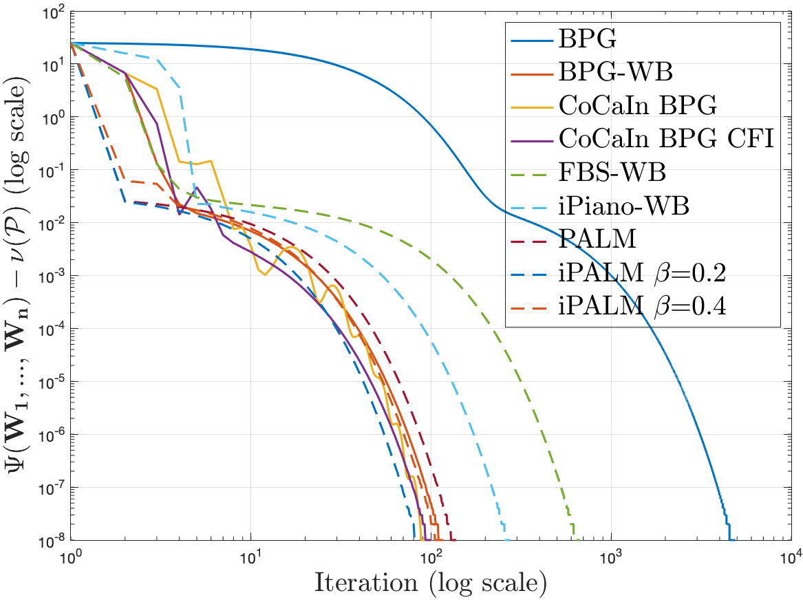
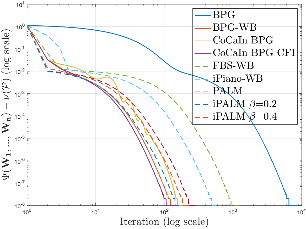
(c) No Regularization ($N=3$)

(d) L2-Regularization ($N=4$)

(e) L1-Regularization ($N=4$)

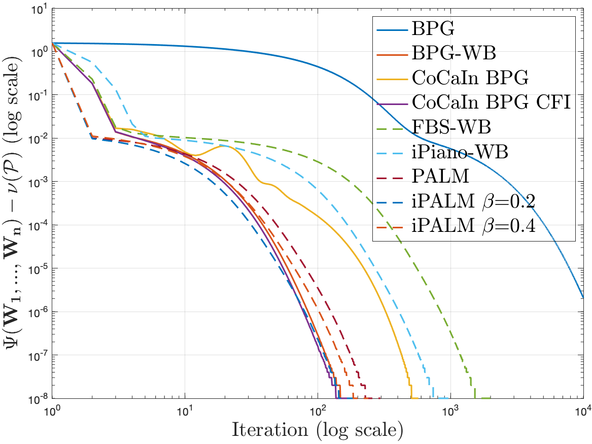
(f) No Regularization ($N=4$)

(g) L2-Regularization ($N=5$)

(h) L1-Regularization ($N=5$)

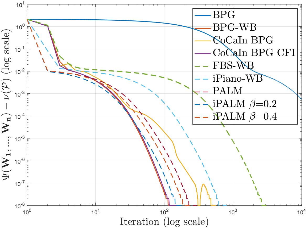
(i) No Regularization ($N=5$)

Figure 1: Convergence plots illustrate the competitive performance of CoCaIn BPG variants for DLNN.

We provide experiments for Deep Linear Neural Networks with squared L2-regularizer and L1-regularizers and a non-regularized setting (3.1).

Algorithms. In the experiments, we compare BPG (Algorithm 1) and CoCaIn BPG (Algorithm 2) with many existing optimization methods. We consider alternating strategies such as PALM [9] and iPALM [30]. As non-alternating algorithms, we use forward backward splitting with backtracking (FBS-WB) and iPiano with backtracking (iPiano-WB) [29]. Apart from BPG and backtracking based CoCaIn BPG, we also inspect CoCaIn BPG with closed form inertia denoted as CoCaIn BPG CFI (see Proposition 11) and the backtracking scheme BPG-WB, which is the same version as CoCaIn BPG, but with $\gamma_{k}\equiv 0$.

Experiment. We set ${\bf W_{i}}\in\mathbb{R}^{5\times 5},~{}\forall i=1,...,N$ where all weights are initialized with $0.1$. Our dataset contains 50 data points with the input ${\bf X}\in\mathbb{R}^{5\times 50}$ and the output ${\bf Y}\in\mathbb{R}^{5\times 50}$ being randomly generated in the interval $[0,1]$. In this experiment, we work with a network consisting of three, four and five layers ($N=3,4,5$). The convergence plots are given in Figure 1, where the $y$-axis measures difference between the absolute objective and the least objective value attained by any of the methods.

Analysis. The performance of CoCaIn BPG, CoCaIn BPG CFI and BPG-WB is mostly better than other methods. The next competitive algorithms include FBS-WB and iPiano-WB, followed by PALM and iPALM. The performance of the alternating algorithms strongly depends on the usage of a regularizer, whereas BPG-WB is competitive in both settings. At first glance, it might appear that the performance of BPG is weaker compared to CoCaIn BPG, BPG-WB, FBS-WB, iPiano-WB and other methods. However, note that line search techniques may not be always desirable in practical scenarios, because line search requires multiple objective evaluations, which can involve computationally expensive matrix multiplications (see Section 5). Moreover, PALM and iPALM require block-wise Lipschitz constant computations in each iteration, which can also be very expensive.

In the appendix, we further illustrate the competitiveness of our methods with time plots, the statistical evaluation and results for an additional dataset.

Conclusion and Extensions

We proposed new Bregman distances suitable for deep linear neural networks. This result makes BPG and its inertial variant CoCaIn BPG applicable and enables the transfer of their convergence results to such problems. Moreover, we develop update formulas, which are crucial for efficient large scale optimization. In general, the validity of inertial (or momentum) parameter requires to be checked via backtracking line search. To avoid expensive backtracking operation, we derive a analytic expression. These contributions serve as a first step towards the optimization of deep (non-linear) neural networks by a new class of Bregman Proximal algorithms.

Appendix

Appendix A Bregman distance and $L$-smad property

Proposition 12.

Denote $g({\bf W_{1}},\ldots,{\bf W_{N}}):=\frac{1}{2}\left\|{{\bf W_{1}W_{2}\ldots W_{N}X}-{\bf Y}}\right\|^{2}_{F}$ as in the setting of (3.1). Then the gradient with respect to weights ${\bf W_{i}}$ is given by

$$\nabla_{{\bf W_{i}}}g({\bf W_{1}},\ldots,{\bf W_{N}})=\left(\Pi_{j=1}^{i-1}{\bf W_{j}}\right)^{T}\left({\bf W_{1}W_{2}\ldots W_{N}X}-{\bf Y}\right)\left(\left(\Pi_{j=i+1}^{N}{\bf W_{j}}\right){\bf X}\right)^{T}\,.$$

We have for $N=2$,

$$\left\langle{({\bf H}_{{\bf 1}},\ldots,{\bf H}_{{\bf N}}),\nabla^{2}g({\bf W_{1}},\ldots,{\bf W_{N}})({\bf H}_{{\bf 1}},\ldots,{\bf H}_{{\bf N}})}\right\rangle$$

$$\leq 3\left\|{\bf X}\right\|_{F}^{2}\sum_{i=1}^{N}\left\|{{\bf H_{i}}}\right\|_{F}^{2}\Pi_{j=1,j\neq i}^{N}\left\|{{\bf W_{j}}}\right\|_{F}^{2}+\left\|{{\bf Y}}\right\|_{F}\left\|{\bf X}\right\|_{F}\left(\left\|{{\bf H}_{1}}\right\|_{F}^{2}+\left\|{{\bf H}_{2}}\right\|_{F}^{2}\right)$$

If $N>2$ and even, we have

$$\left\langle{({\bf H}_{{\bf 1}},\ldots,{\bf H}_{{\bf N}}),\nabla^{2}g({\bf W_{1}},\ldots,{\bf W_{N}})({\bf H}_{{\bf 1}},\ldots,{\bf H}_{{\bf N}})}\right\rangle$$

$$\leq(2N-1)\sum_{i=1}^{N}\left\|{{\bf H_{i}}}\right\|_{F}^{2}\Pi_{j=1,j\neq i}^{N}\left\|{{\bf W_{j}}}\right\|_{F}^{2}\left\|{\bf X}\right\|_{F}^{2}+\frac{\left\|{{\bf Y}}\right\|_{F}\left\|{\bf X}\right\|_{F}(N-1)}{(N-2)^{\frac{N-2}{2}}}\left(\sum_{i=1}^{N}\left\|{{\bf H}_{i}}\right\|_{F}^{2}\right)\left(\sum_{k=1}^{N}\left\|{\bf W_{k}}\right\|_{F}^{2}\right)^{\frac{N-2}{2}}$$

If $N>2$ and odd, we have

$$\left\langle{({\bf H}_{{\bf 1}},\ldots,{\bf H}_{{\bf N}}),\nabla^{2}g({\bf W_{1}},\ldots,{\bf W_{N}})({\bf H}_{{\bf 1}},\ldots,{\bf H}_{{\bf N}})}\right\rangle$$

$$\leq(2N-1)\sum_{i=1}^{N}\left\|{{\bf H_{i}}}\right\|_{F}^{2}\Pi_{j=1,j\neq i}^{N}\left\|{{\bf W_{j}}}\right\|_{F}^{2}\left\|{\bf X}\right\|_{F}^{2}+\frac{\left\|{{\bf Y}}\right\|_{F}\left\|{\bf X}\right\|_{F}(N-1)}{(N-1)^{\frac{N-1}{2}}}\left(\sum_{i=1}^{N}\left\|{{\bf H}_{i}}\right\|_{F}^{2}\right)\left(\left(\sum_{k=1,k\notin\{i,j\}}^{N}\left\|{\bf W_{k}}\right\|_{F}^{2}\right)+1\right)^{\frac{N-1}{2}}$$

Proof.

Consider the following

$$\frac{1}{2}\left\|{{\bf(W_{1}+H_{1})(W_{2}+H_{2})\ldots(W_{N}+H_{N})X}-{\bf Y}}\right\|^{2}_{F}\,.$$ (A.1)

We are only interested in terms till second order, thus we have

$${\bf(W_{1}+H_{1})(W_{2}+H_{2})\ldots(W_{N}+H_{N})X} ={\bf W_{1}W_{2}\ldots W_{N}X}+\sum_{i=1}^{N}\left(\Pi_{j=1}^{i-1}{\bf W_{j}}\right){\bf H_{i}}\left(\Pi_{j=i+1}^{N}{\bf W_{j}}{\bf X}\right)$$

$$+\sum_{i=1}^{N-1}\sum_{j>i}^{N}\left(\Pi_{k=1}^{i-1}{\bf W_{k}}\right){\bf H_{i}}\left(\Pi_{k=i+1}^{j-1}{\bf W_{k}}\right){\bf H_{j}}\left(\Pi_{k=j+1}^{N}{\bf W_{k}}{\bf X}\right)\,.$$

Now expanding (A.1), we have terms upto second order as following

$$\frac{1}{2}\left\|{{\bf W_{1}W_{2}\ldots W_{N}X}-{\bf Y}}\right\|_{F}^{2}+\left\langle{{\bf W_{1}W_{2}\ldots W_{N}X}-{\bf Y},\sum_{i=1}^{N}\left(\Pi_{j=1}^{i-1}{\bf W_{j}}\right){\bf H_{i}}\left(\Pi_{j=i+1}^{N}{\bf W_{j}}\right){\bf X}}\right\rangle$$

$$+\frac{1}{2}\left\|{\sum_{i=1}^{N}\left(\Pi_{j=1}^{i-1}{\bf W_{j}}\right){\bf H_{i}}\left(\Pi_{j=i+1}^{N}{\bf W_{j}}\right){\bf X}}\right\|_{F}^{2}-\left\langle{{\bf Y},\sum_{i=1}^{N-1}\sum_{j>i}^{N}\left(\Pi_{k=1}^{i-1}{\bf W_{k}}\right){\bf H_{i}}\left(\Pi_{k=i+1}^{j-1}{\bf W_{k}}\right){\bf H_{j}}\left(\Pi_{k=j+1}^{N}{\bf W_{k}}\right){\bf X}}\right\rangle$$

$$+\left\langle{{\bf W_{1}W_{2}\ldots W_{N}X},\sum_{i=1}^{N-1}\sum_{j>i}^{N}\left(\Pi_{k=1}^{i-1}{\bf W_{k}}\right){\bf H_{i}}\left(\Pi_{k=i+1}^{j-1}{\bf W_{k}}\right){\bf H_{j}}\left(\Pi_{k=j+1}^{N}{\bf W_{k}}\right){\bf X}}\right\rangle\,.$$

Consider the first order terms, we have

$$\left\langle{{\bf W_{1}W_{2}\ldots W_{N}X}-{\bf Y},\sum_{i=1}^{N}\left(\Pi_{j=1}^{i-1}{\bf W_{j}}\right){\bf H_{i}}\left(\Pi_{j=i+1}^{N}{\bf W_{j}}\right){\bf X}}\right\rangle$$

$$=\sum_{i=1}^{N}\left\langle{{\bf W_{1}W_{2}\ldots W_{N}X}-{\bf Y},\left(\Pi_{j=1}^{i-1}{\bf W_{j}}\right){\bf H_{i}}\left(\Pi_{j=i+1}^{N}{\bf W_{j}}\right){\bf X}}\right\rangle\,,$$

thus, the gradient is

$$\nabla_{{\bf W_{i}}}g({\bf W_{1}},\ldots,{\bf W_{N}})=\left(\Pi_{j=1}^{i-1}{\bf W_{j}}\right)^{T}\left({\bf W_{1}W_{2}\ldots W_{N}X}-{\bf Y}\right)\left(\left(\Pi_{j=i+1}^{N}{\bf W_{j}}\right){\bf X}\right)^{T}\,.$$

Now, considering second order terms we have with repetitive application of Cauchy-Schwarz inequality, the following

$$\frac{1}{2}\left\|{\sum_{i=1}^{N}\left(\Pi_{j=1}^{i-1}{\bf W_{j}}\right){\bf H_{i}}\left(\Pi_{j=i+1}^{N}{\bf W_{j}}\right){\bf X}}\right\|_{F}^{2} \leq\frac{N}{2}\sum_{i=1}^{N}\left\|{\left(\Pi_{j=1}^{i-1}{\bf W_{j}}\right){\bf H_{i}}\left(\Pi_{j=i+1}^{N}{\bf W_{j}}\right){\bf X}}\right\|_{F}^{2}$$

$$\leq\frac{N}{2}\sum_{i=1}^{N}\left\|{{\bf H_{i}}}\right\|_{F}^{2}\Pi_{j=1,j\neq i}^{N}\left\|{{\bf W_{j}}}\right\|_{F}^{2}\left\|{\bf X}\right\|_{F}^{2}$$

and

$$\left\langle{{\bf W_{1}W_{2}\ldots W_{N}X},\sum_{i=1}^{N-1}\sum_{j>i}^{N}\left(\Pi_{k=1}^{i-1}{\bf W_{k}}\right){\bf H_{i}}\left(\Pi_{k=i+1}^{j-1}{\bf W_{k}}\right){\bf H_{j}}\left(\Pi_{k=j+1}^{N}{\bf W_{k}}\right){\bf X}}\right\rangle$$

$$\leq\sum_{i=1}^{N-1}\sum_{j>i}^{N}\left\|{{\bf X}}\right\|_{F}^{2}\left\|{{\bf H}_{i}}\right\|_{F}\left\|{{\bf H}_{j}}\right\|_{F}\left\|{{\bf W_{i}}}\right\|_{F}\left\|{{\bf W_{j}}}\right\|_{F}\Pi_{k=1,k\notin\{i,j\}}^{N}\left\|{\bf W_{k}}\right\|_{F}^{2}$$

$$\leq\sum_{i=1}^{N-1}\sum_{j>i}^{N}\left\|{{\bf X}}\right\|_{F}^{2}\left(\frac{\left\|{{\bf H}_{i}}\right\|_{F}^{2}\left\|{{\bf W_{j}}}\right\|_{F}^{2}+\left\|{{\bf H}_{j}}\right\|_{F}^{2}\left\|{{\bf W_{i}}}\right\|_{F}^{2}}{2}\right)\Pi_{k=1,k\notin\{i,j\}}^{N}\left\|{\bf W_{k}}\right\|_{F}^{2}$$

$$\leq\left\|{{\bf X}}\right\|_{F}^{2}\left(\frac{N-1}{2}\right)\sum_{i=1}^{N}\left\|{{\bf H}_{i}}\right\|_{F}^{2}\Pi_{k=1,k\notin\{i\}}^{N}\left\|{\bf W_{k}}\right\|_{F}^{2}$$

and we have

$$-\left\langle{{\bf Y},\sum_{i=1}^{N-1}\sum_{j>i}^{N}\left(\Pi_{k=1}^{i-1}{\bf W_{k}}\right){\bf H_{i}}\left(\Pi_{k=i+1}^{j-1}{\bf W_{k}}\right){\bf H_{j}}\left(\Pi_{k=j+1}^{N}{\bf W_{k}}\right){\bf X}}\right\rangle$$

$$\leq\left\|{{\bf Y}}\right\|_{F}\sum_{i=1}^{N-1}\sum_{j>i}^{N}\left\|{{\bf H}_{i}}\right\|_{F}\left\|{{\bf H}_{j}}\right\|_{F}\Pi_{k=1,k\notin\{i,j\}}^{N}\left\|{\bf W_{k}}\right\|_{F}\left\|{\bf X}\right\|_{F}$$ (A.2)

Now with the application of Generalized AM-GM inequality, we have the following three cases:

• When $N=2$ then we have

  $$\left\|{{\bf H}_{i}}\right\|_{F}\left\|{{\bf H}_{j}}\right\|_{F}\left\|{\bf X}\right\|_{F}\leq\left\|{\bf X}\right\|_{F}\left(\frac{\left\|{{\bf H}_{j}}\right\|_{F}^{2}+\left\|{{\bf H}_{i}}\right\|_{F}^{2}}{2}\right)\,,$$

• When $N$ is even and $N>2$.

  $$\left\|{{\bf H}_{i}}\right\|_{F}\left\|{{\bf H}_{j}}\right\|_{F}\Pi_{k=1,k\notin\{i,j\}}^{N}\left\|{\bf W_{k}}\right\|_{F}\left\|{\bf X}\right\|_{F}\leq\left\|{\bf X}\right\|_{F}\left(\frac{\left\|{{\bf H}_{j}}\right\|_{F}^{2}+\left\|{{\bf H}_{i}}\right\|_{F}^{2}}{2}\right)\left(\frac{\sum_{k=1,k\notin\{i,j\}}^{N}\left\|{\bf W_{k}}\right\|_{F}^{2}}{N-2}\right)^{\frac{N-2}{2}}\,,$$

• If $N$ is odd and $N>2$ we have

  $$\left\|{{\bf H}_{i}}\right\|_{F}\left\|{{\bf H}_{j}}\right\|_{F}\Pi_{k=1,k\notin\{i,j\}}^{N}\left\|{\bf W_{k}}\right\|_{F}\left\|{\bf X}\right\|_{F}\leq\left\|{\bf X}\right\|_{F}\left(\frac{\left\|{{\bf H}_{j}}\right\|_{F}^{2}+\left\|{{\bf H}_{i}}\right\|_{F}^{2}}{2}\right)\left(\frac{\left(\sum_{k=1,k\notin\{i,j\}}^{N}\left\|{\bf W_{k}}\right\|_{F}^{2}\right)+1}{N-1}\right)^{\frac{N-1}{2}}\,.$$

Now using the above given results, on extending the calculation of (A.2), for even $N$ and $N\geq 2$, we have

$$\left\|{{\bf Y}}\right\|_{F}\sum_{i=1}^{N-1}\sum_{j>i}^{N}\left\|{{\bf H}_{i}}\right\|_{F}\left\|{{\bf H}_{j}}\right\|_{F}\Pi_{k=1,k\notin\{i,j\}}^{N}\left\|{\bf W_{k}}\right\|_{F}\left\|{\bf X}\right\|_{F}$$

$$\leq\left\|{{\bf Y}}\right\|_{F}\left\|{\bf X}\right\|_{F}\sum_{i=1}^{N-1}\sum_{j>i}^{N}\left(\frac{\left\|{{\bf H}_{j}}\right\|_{F}^{2}+\left\|{{\bf H}_{i}}\right\|_{F}^{2}}{2}\right)\left(\frac{\sum_{k=1,k\notin\{i,j\}}^{N}\left\|{\bf W_{k}}\right\|_{F}^{2}}{N-2}\right)^{\frac{N-2}{2}}$$

$$\leq\frac{\left\|{{\bf Y}}\right\|_{F}\left\|{\bf X}\right\|_{F}(N-1)}{2(N-2)^{\frac{N-2}{2}}}\left(\sum_{i=1}^{N}\left\|{{\bf H}_{i}}\right\|_{F}^{2}\right)\left(\sum_{k=1}^{N}\left\|{\bf W_{k}}\right\|_{F}^{2}\right)^{\frac{N-2}{2}}\,,$$

where in the first step we used Cauchy-Schwarz inequality. Similarly, we have for $N>2$ and odd,

$$\left\|{{\bf Y}}\right\|_{F}\sum_{i=1}^{N-1}\sum_{j>i}^{N}\left\|{{\bf H}_{i}}\right\|_{F}\left\|{{\bf H}_{j}}\right\|_{F}\Pi_{k=1,k\notin\{i,j\}}^{N}\left\|{\bf W_{k}}\right\|_{F}\left\|{\bf X}\right\|_{F}$$

$$\leq\left\|{{\bf Y}}\right\|_{F}\left\|{\bf X}\right\|_{F}\sum_{i=1}^{N-1}\sum_{j>i}^{N}\left(\frac{\left\|{{\bf H}_{j}}\right\|_{F}^{2}+\left\|{{\bf H}_{i}}\right\|_{F}^{2}}{2}\right)\left(\frac{\left(\sum_{k=1,k\notin\{i,j\}}^{N}\left\|{\bf W_{k}}\right\|_{F}^{2}\right)+1}{N-1}\right)^{\frac{N-1}{2}}$$

$$\leq\frac{\left\|{{\bf Y}}\right\|_{F}\left\|{\bf X}\right\|_{F}(N-1)}{2(N-1)^{\frac{N-1}{2}}}\left(\sum_{i=1}^{N}\left\|{{\bf H}_{i}}\right\|_{F}^{2}\right)\left(\left(\sum_{k=1}^{N}\left\|{\bf W_{k}}\right\|_{F}^{2}\right)+1\right)^{\frac{N-1}{2}}\,.$$

∎

Before we start with the proof of Proposition 7, we require the following technical results.

A.1 Results for $H_{1}$.

Lemma 13.

Let $h\in\mathcal{G}(C)$ be twice continuously differentiable on $C$. Then, the following identity holds

$$D_{h}(x^{k},y^{k})=\int_{0}^{1}\left(1-t\right)\int_{0}^{1}\left\langle{\nabla^{2}h\left(x^{k}+(t_{1}+(1-t_{1})t)(y^{k}-x^{k})\right)(x^{k}-y^{k}),x^{k}-y^{k}}\right\rangle dt_{1}dt\,.$$

Proof.

With repetitive application of fundamental theorem of calculus we have

$$h(x^{k})-h(y^{k})-\left\langle{\nabla h(y^{k}),x^{k}-y^{k}}\right\rangle$$

$$=\int_{0}^{1}\left\langle{\nabla h(x^{k}+t(y^{k}-x^{k}))-\nabla h(y^{k}),x^{k}-y^{k}}\right\rangle dt\,,$$

$$=\int_{0}^{1}\left\langle{\int_{0}^{1}\nabla^{2}h\left((1-t_{1})(x^{k}+t(y^{k}-x^{k}))+t_{1}y^{k}\right)\left(1-t\right)(x^{k}-y^{k})dt_{1},x^{k}-y^{k}}\right\rangle dt\,,$$

$$=\int_{0}^{1}\left\langle{\int_{0}^{1}\nabla^{2}h\left(x^{k}+(t_{1}+(1-t_{1})t)(y^{k}-x^{k})\right)\left(1-t\right)(x^{k}-y^{k})dt_{1},x^{k}-y^{k}}\right\rangle dt\,,$$

$$=\int_{0}^{1}\left(1-t\right)\int_{0}^{1}\left\langle{\nabla^{2}h\left(x^{k}+(t_{1}+(1-t_{1})t)(y^{k}-x^{k})\right)(x^{k}-y^{k}),x^{k}-y^{k}}\right\rangle dt_{1}dt\,.$$

∎

Henceforth, we use the following notation. Let $n$ be a positive integer and let $k_{i}$ be a non-negative integer for $i\in[m]$ satisfying $k_{1}+\ldots+k_{m}=n$, then we denote

$$\binom{n}{k_{1},k_{2},\ldots,k_{m}}:=\frac{n!}{k_{1}!k_{2}!\ldots k_{m}!}\,,$$

which is also known as multinomial coefficient.

Lemma 14.

With the following kernel generating distance

$$H_{1}({\bf W_{1}},\ldots,{\bf W_{N}})=\left(\frac{\left\|{{\bf W_{1}}}\right\|_{F}^{2}+\ldots\left\|{{\bf W_{N}}}\right\|_{F}^{2}}{N}\right)^{N}\,,$$

the gradient with respect for ${\bf W_{i}}$, for any $i\in[N]$, is given by

$$\nabla_{{\bf W_{i}}}H_{1}({\bf W_{1}},\ldots,{\bf W_{N}})=\frac{2}{N^{N}}\binom{N}{N-1,1}\left(\left\|{{\bf W_{1}}}\right\|_{F}^{2}+\ldots+\left\|{{\bf W_{N}}}\right\|_{F}^{2}\right)^{N-1}{\bf W_{i}}\,,$$

and the following lower bound holds true

$$\left\langle{({\bf H}_{{\bf 1}},\ldots,{\bf H}_{{\bf N}}),\nabla^{2}H_{1}({\bf W_{1}},\ldots,{\bf W_{N}})({\bf H}_{{\bf 1}},\ldots,{\bf H}_{{\bf N}})}\right\rangle\geq\frac{2N!}{N^{N}}\sum_{i=1}^{N}\left\|{{\bf H}_{i}}\right\|_{F}^{2}\Pi_{k=1,k\notin\{i\}}^{N}\left\|{\bf W_{k}}\right\|_{F}^{2}\,,$$

and the following upper bound holds true

$$\left\langle{({\bf H}_{{\bf 1}},\ldots,{\bf H}_{{\bf N}}),\nabla^{2}H_{1}({\bf W_{1}},\ldots,{\bf W_{N}})({\bf H}_{{\bf 1}},\ldots,{\bf H}_{{\bf N}})}\right\rangle\leq\left(\frac{2(2N-1)}{N^{N-1}}\right)\left(\sum_{k=1}^{N}\left\|{{\bf H_{k}}}\right\|_{F}^{2}\right)\left(\sum_{k=1}^{N}\left\|{\bf W_{k}}\right\|_{F}^{2}\right)^{N-1}\,.$$

Proof.

Consider the following

$$\left(\frac{\left\|{{\bf W_{1}}+{\bf H_{1}}}\right\|_{F}^{2}+\ldots\left\|{{\bf W_{N}}+{\bf H_{N}}}\right\|_{F}^{2}}{N}\right)^{N}=\left(\frac{\left\|{{\bf W_{1}}}\right\|_{F}^{2}+\left\|{{\bf H_{1}}}\right\|_{F}^{2}+2\left\langle{{\bf W_{1}},{\bf H_{1}}}\right\rangle+\ldots\left\|{{\bf W_{N}}}\right\|_{F}^{2}+\left\|{{\bf H_{N}}}\right\|_{F}^{2}}{N}\right)^{N}\,.$$

Consider only the first order terms in the expansion, from which the following gradient with respect for ${\bf W_{i}}$, for any $i\in[N]$, is obtained

$$\nabla_{{\bf W_{i}}}H_{1}({\bf W_{1}},\ldots,{\bf W_{N}})=\frac{2}{N^{N}}\binom{N}{N-1,1}\left(\left\|{{\bf W_{1}}}\right\|_{F}^{2}+\ldots+\left\|{{\bf W_{N}}}\right\|_{F}^{2}\right)^{N-1}{\bf W_{i}}\,.$$

Now considering only the second order terms, we have

$$\frac{1}{2}\left\langle{({\bf H}_{{\bf 1}},\ldots,{\bf H}_{{\bf N}}),\nabla^{2}H_{1}({\bf W_{1}},\ldots,{\bf W_{N}})({\bf H}_{{\bf 1}},\ldots,{\bf H}_{{\bf N}})}\right\rangle$$

$$=\frac{1}{2}\frac{2}{N^{N}}\sum_{i=1}^{N}\binom{N}{1,N-1}\left\|{{\bf H}_{i}}\right\|_{F}^{2}\left(\sum_{k=1}^{N}\left\|{\bf W_{k}}\right\|_{F}^{2}\right)^{N-1}$$

$$+\frac{1}{2}\frac{2^{3}}{N^{N}}\binom{N}{2,N-2}\left(\left\langle{{\bf W_{1}},{\bf H_{1}}}\right\rangle+\ldots+\left\langle{{\bf W_{N}},{\bf H_{N}}}\right\rangle\right)^{2}\left(\sum_{k=1}^{N}\left\|{\bf W_{k}}\right\|_{F}^{2}\right)^{N-2}\,.$$

Since, the second term in the right hand side is always non-negative, the following result holds

$$\frac{1}{2}\left\langle{({\bf H}_{{\bf 1}},\ldots,{\bf H}_{{\bf N}}),\nabla^{2}H_{1}({\bf W_{1}},\ldots,{\bf W_{N}})({\bf H}_{{\bf 1}},\ldots,{\bf H}_{{\bf N}})}\right\rangle\geq\frac{1}{2}\frac{2N!}{N^{N}}\sum_{i=1}^{N}\left\|{{\bf H}_{i}}\right\|_{F}^{2}\Pi_{k=1,k\notin\{i\}}^{N}\left\|{\bf W_{k}}\right\|_{F}^{2}\,.$$

This proves the lower bound. Now, we prove the upper bound. With application of Cauchy-Schwarz inequality, we have

$$\frac{1}{2}\frac{2^{3}}{N^{N}}\binom{N}{2,N-2}\left(\left\langle{{\bf W_{1}},{\bf H_{1}}}\right\rangle+\ldots+\left\langle{{\bf W_{N}},{\bf H_{N}}}\right\rangle\right)^{2}\left(\sum_{k=1}^{N}\left\|{\bf W_{k}}\right\|_{F}^{2}\right)^{N-2}$$

$$\leq\frac{1}{2}\frac{2^{3}}{N^{N}}\binom{N}{2,N-2}\left(\sum_{k=1}^{N}\left\|{{\bf W_{k}}}\right\|_{F}^{2}\right)\left(\sum_{k=1}^{N}\left\|{{\bf H_{k}}}\right\|_{F}^{2}\right)\left(\sum_{k=1}^{N}\left\|{\bf W_{k}}\right\|_{F}^{2}\right)^{N-2}$$

$$=\frac{1}{2}\frac{2^{3}}{N^{N}}\binom{N}{2,N-2}\left(\sum_{k=1}^{N}\left\|{{\bf H_{k}}}\right\|_{F}^{2}\right)\left(\sum_{k=1}^{N}\left\|{\bf W_{k}}\right\|_{F}^{2}\right)^{N-1}\,.$$

Now we finally have

$$\left\langle{({\bf H}_{{\bf 1}},\ldots,{\bf H}_{{\bf N}}),\nabla^{2}H_{1}({\bf W_{1}},\ldots,{\bf W_{N}})({\bf H}_{{\bf 1}},\ldots,{\bf H}_{{\bf N}})}\right\rangle \leq\frac{2}{N^{N}}\binom{N}{1,N-1}\left(\sum_{i=1}^{N}\left\|{{\bf H}_{i}}\right\|_{F}^{2}\right)\left(\sum_{k=1}^{N}\left\|{\bf W_{k}}\right\|_{F}^{2}\right)^{N-1}$$

$$+\frac{2^{3}}{N^{N}}\binom{N}{2,N-2}\left(\sum_{k=1}^{N}\left\|{{\bf H_{k}}}\right\|_{F}^{2}\right)\left(\sum_{k=1}^{N}\left\|{\bf W_{k}}\right\|_{F}^{2}\right)^{N-1}$$

$$=\left(\frac{2(2N-1)}{N^{N-1}}\right)\left(\sum_{k=1}^{N}\left\|{{\bf H_{k}}}\right\|_{F}^{2}\right)\left(\sum_{k=1}^{N}\left\|{\bf W_{k}}\right\|_{F}^{2}\right)^{N-1}\,.\qed$$

Lemma 15.

Denote for any $k\geq 1$, $x^{k}=({\bf W_{1}^{k}},\ldots,{\bf W_{N}^{k}})$, $\Delta_{k}:={x^{k}-x^{k-1}}$ and the following

$$\mathcal{B}_{k}:= \left(\frac{(2N-1)}{N^{N-1}}\right)\left\|{\Delta_{k}}\right\|^{2}\left(2\left\|{x^{k}}\right\|^{2}+2\left\|{\Delta_{k}}\right\|^{2}\right)^{(N-1)}\,.$$

The following upper bound holds true

$$D_{H_{1}}(x^{k},y^{k})\leq\gamma_{k}^{2}\mathcal{B}_{k}\,.$$

Proof.

From Lemma 13, we have

$$\int_{0}^{1}\left(1-t\right)\int_{0}^{1}\left\langle{\nabla^{2}H_{1}\left(x^{k}+(t_{1}+(1-t_{1})t)(y^{k}-x^{k})\right)(x^{k}-y^{k}),x^{k}-y^{k}}\right\rangle dt_{1}dt$$

$$= \gamma_{k}^{2}\int_{0}^{1}\left(1-t\right)\int_{0}^{1}\left\langle{\nabla^{2}H_{1}\left(x^{k}+(t_{1}+(1-t_{1})t)(y^{k}-x^{k})\right)(x^{k}-x^{k-1}),x^{k}-x^{k-1}}\right\rangle dt_{1}dt\,,$$

$$\leq \gamma_{k}^{2}\int_{0}^{1}\left(1-t\right)\int_{0}^{1}\frac{2(2N-1)}{N^{N-1}}\left\|{x^{k}-x^{k-1}}\right\|^{2}\left\|{x^{k}+(t_{1}+(1-t_{1})t)(y^{k}-x^{k})}\right\|^{(2N-2)}dt_{1}dt\,,$$

where in the last step we used the upper bound from Lemma 14. Using the following inequality

$$\left\|{x^{k}+(t_{1}+(1-t_{1})t)(y^{k}-x^{k})}\right\|^{2} \leq 2\left\|{x^{k}}\right\|^{2}+2(t_{1}+(1-t_{1})t)^{2}\gamma_{k}^{2}\left\|{x^{k}-x^{k-1}}\right\|^{2}\leq 2\left\|{x^{k}}\right\|^{2}+2\left\|{x^{k}-x^{k-1}}\right\|^{2}$$

where in the last step we used $\gamma_{k}^{2}\leq 1$ and $(t_{1}+(1-t_{1})t)^{2}\leq 1$. With $\int_{0}^{1}(1-t)dt=\frac{1}{2}$ the result follows.∎

A.2 Results for $H_{2}$.

Lemma 16.

With the following kernel generating distance

$$H_{2}({\bf W_{1}},\ldots,{\bf W_{N}})=\left(\frac{\left\|{{\bf W_{1}}}\right\|_{F}^{2}+\left\|{{\bf W_{2}}}\right\|_{F}^{2}+\ldots\left\|{{\bf W_{N}}}\right\|_{F}^{2}}{N}\right)^{\frac{N}{2}}\,,$$

the gradient with respect for ${\bf W_{i}}$, for any $i\in[N]$, is given by

$$\nabla_{{\bf W_{i}}}H_{2}({\bf W_{1}},\ldots,{\bf W_{N}})=\frac{1}{N^{\frac{N}{2}-1}}\left(\left\|{{\bf W_{1}}}\right\|_{F}^{2}+\ldots+\left\|{{\bf W_{N}}}\right\|_{F}^{2}\right)^{{\frac{N}{2}}-1}{\bf W_{i}}\,,$$

and the following lower bound holds true

$$\left\langle{({\bf H}_{{\bf 1}},\ldots,{\bf H}_{{\bf N}}),\nabla^{2}H_{2}({\bf W_{1}},\ldots,{\bf W_{N}})({\bf H}_{{\bf 1}},\ldots,{\bf H}_{{\bf N}})}\right\rangle\geq\frac{1}{N^{\frac{N}{2}-1}}\left(\left\|{{\bf H}_{1}}\right\|_{F}^{2}+\ldots+\left\|{{\bf H}_{N}}\right\|_{F}^{2}\right)\left(\sum_{k=1}^{N}\left\|{\bf W_{k}}\right\|_{F}^{2}\right)^{\frac{N-2}{2}}\,,$$

and the following upper bound holds true

$$\left\langle{({\bf H}_{{\bf 1}},\ldots,{\bf H}_{{\bf N}}),\nabla^{2}H_{2}({\bf W_{1}},\ldots,{\bf W_{N}})({\bf H}_{{\bf 1}},\ldots,{\bf H}_{{\bf N}})}\right\rangle\leq\left(\frac{N-1}{N^{\frac{N}{2}-1}}\right)\left(\sum_{k=1}^{N}\left\|{{\bf H_{k}}}\right\|_{F}^{2}\right)\left(\sum_{k=1}^{N}\left\|{\bf W_{k}}\right\|_{F}^{2}\right)^{\frac{N-2}{2}}\,.$$

Proof.

Consider the following expansion

$$\left(\frac{\left\|{{\bf W_{1}}+{\bf H_{1}}}\right\|_{F}^{2}+\ldots\left\|{{\bf W_{N}}+{\bf H_{N}}}\right\|_{F}^{2}}{N}\right)^{\frac{N}{2}}=\left(\frac{\left\|{{\bf W_{1}}}\right\|_{F}^{2}+\left\|{{\bf H_{1}}}\right\|_{F}^{2}+2\left\langle{{\bf W_{1}},{\bf H_{1}}}\right\rangle+\ldots\left\|{{\bf W_{N}}}\right\|_{F}^{2}+\left\|{{\bf H_{N}}}\right\|_{F}^{2}}{N}\right)^{\frac{N}{2}}\,.$$

Consider only the first order terms in the expansion, from which the following gradient with respect for ${\bf W_{i}}$, for any $i\in[N]$, is obtained

$$\nabla_{{\bf W_{i}}}H_{2}({\bf W_{1}},\ldots,{\bf W_{N}})=\frac{2}{N^{\frac{N}{2}}}\binom{\frac{N}{2}}{{\frac{N}{2}}-1,1}\left(\left\|{{\bf W_{1}}}\right\|_{F}^{2}+\ldots+\left\|{{\bf W_{N}}}\right\|_{F}^{2}\right)^{{\frac{N}{2}}-1}{\bf W_{i}}\,.$$

Now considering only the second order terms, we have

$$\frac{1}{2}\left\langle{({\bf H}_{{\bf 1}},\ldots,{\bf H}_{{\bf N}}),\nabla^{2}H_{2}({\bf W_{1}},\ldots,{\bf W_{N}})({\bf H}_{{\bf 1}},\ldots,{\bf H}_{{\bf N}})}\right\rangle$$

$$=\frac{1}{2}\frac{2}{N^{\frac{N}{2}}}\binom{\frac{N}{2}}{\frac{N-2}{2},1}\left(\left\|{{\bf H}_{1}}\right\|_{F}^{2}+\ldots+\left\|{{\bf H}_{N}}\right\|_{F}^{2}\right)\left(\sum_{k=1}^{N}\left\|{\bf W_{k}}\right\|_{F}^{2}\right)^{\frac{N-2}{2}}$$

$$+\frac{1}{2}\frac{2^{3}}{N^{\frac{N}{2}}}\binom{\frac{N}{2}}{2,\frac{N}{2}-2}\left(\left\langle{{\bf W_{1}},{\bf H_{1}}}\right\rangle+\ldots+\left\langle{{\bf W_{N}},{\bf H_{N}}}\right\rangle\right)^{2}\left(\sum_{k=1}^{N}\left\|{\bf W_{k}}\right\|_{F}^{2}\right)^{\frac{N}{2}-2}$$

Since, the second term in the right hand side is always non-negative, the following result holds

$$\left\langle{({\bf H}_{{\bf 1}},\ldots,{\bf H}_{{\bf N}}),\nabla^{2}H_{2}({\bf W_{1}},\ldots,{\bf W_{N}})({\bf H}_{{\bf 1}},\ldots,{\bf H}_{{\bf N}})}\right\rangle\geq\frac{2}{N^{\frac{N}{2}}}\binom{\frac{N}{2}}{\frac{N-2}{2},1}\left(\left\|{{\bf H}_{1}}\right\|_{F}^{2}+\ldots+\left\|{{\bf H}_{N}}\right\|_{F}^{2}\right)\left(\sum_{k=1}^{N}\left\|{\bf W_{k}}\right\|_{F}^{2}\right)^{\frac{N-2}{2}}\,.$$

This proves the lower bound as in the statement. Now we prove the upper bound. With application of Cauchy-Schwarz inequality, we have

$$\frac{1}{2}\frac{2^{3}}{N^{\frac{N}{2}}}\binom{\frac{N}{2}}{2,\frac{N}{2}-2}\left(\left\langle{{\bf W_{1}},{\bf H_{1}}}\right\rangle+\ldots+\left\langle{{\bf W_{N}},{\bf H_{N}}}\right\rangle\right)^{2}\left(\sum_{k=1}^{N}\left\|{\bf W_{k}}\right\|_{F}^{2}\right)^{\frac{N}{2}-2}$$

$$\leq\frac{1}{2}\frac{2^{3}}{N^{\frac{N}{2}}}\binom{\frac{N}{2}}{2,\frac{N}{2}-2}\left(\sum_{k=1}^{N}\left\|{{\bf W_{k}}}\right\|_{F}^{2}\right)\left(\sum_{k=1}^{N}\left\|{{\bf H_{k}}}\right\|_{F}^{2}\right)\left(\sum_{k=1}^{N}\left\|{\bf W_{k}}\right\|_{F}^{2}\right)^{\frac{N}{2}-2}\,,$$

$$=\frac{1}{2}\frac{2^{3}}{N^{\frac{N}{2}}}\binom{\frac{N}{2}}{2,\frac{N}{2}-2}\left(\sum_{k=1}^{N}\left\|{{\bf H_{k}}}\right\|_{F}^{2}\right)\left(\sum_{k=1}^{N}\left\|{\bf W_{k}}\right\|_{F}^{2}\right)^{\frac{N}{2}-1}\,.$$

Thus, we finally have

$$\left\langle{({\bf H}_{{\bf 1}},\ldots,{\bf H}_{{\bf N}}),\nabla^{2}H_{2}({\bf W_{1}},\ldots,{\bf W_{N}})({\bf H}_{{\bf 1}},\ldots,{\bf H}_{{\bf N}})}\right\rangle \leq\frac{2}{N^{\frac{N}{2}}}\binom{\frac{N}{2}}{\frac{N-2}{2},1}\left(\sum_{k=1}^{N}\left\|{{\bf H_{k}}}\right\|_{F}^{2}\right)\left(\sum_{k=1}^{N}\left\|{\bf W_{k}}\right\|_{F}^{2}\right)^{\frac{N-2}{2}}$$

$$+\frac{2^{3}}{N^{\frac{N}{2}}}\binom{\frac{N}{2}}{2,\frac{N}{2}-2}\left(\sum_{k=1}^{N}\left\|{{\bf H_{k}}}\right\|_{F}^{2}\right)\left(\sum_{k=1}^{N}\left\|{\bf W_{k}}\right\|_{F}^{2}\right)^{\frac{N-2}{2}}\,,$$

$$=\left(\frac{N-1}{N^{\frac{N}{2}-1}}\right)\left(\sum_{k=1}^{N}\left\|{{\bf H_{k}}}\right\|_{F}^{2}\right)\left(\sum_{k=1}^{N}\left\|{\bf W_{k}}\right\|_{F}^{2}\right)^{\frac{N-2}{2}}\,.\qed$$

Lemma 17.

Denote for any $k\geq 1$, $x^{k}=({\bf W_{1}^{k}},\ldots,{\bf W_{N}^{k}})$, $\Delta_{k}:={x^{k}-x^{k-1}}$ and the following

$$\mathcal{C}_{k} :=\left(\frac{N-1}{N^{\frac{N}{2}-1}}\right)\left\|{\Delta_{k}}\right\|^{2}\left(2\left\|{x^{k}}\right\|^{2}+2\left\|{\Delta}\right\|^{2}\right)^{\frac{N-2}{2}}\,.$$

The following holds

$$D_{H_{2}}(x^{k},y^{k})\leq\gamma_{k}^{2}\mathcal{C}_{k}\,.$$

Proof.

From Lemma 13, we have

$$\int_{0}^{1}\left(1-t\right)\int_{0}^{1}\left\langle{\nabla^{2}H_{2}\left(x^{k}+(t_{1}+(1-t_{1})t)(y^{k}-x^{k})\right)(x^{k}-y^{k}),x^{k}-y^{k}}\right\rangle dt_{1}dt$$

$$=\gamma_{k}^{2}\int_{0}^{1}\left(1-t\right)\int_{0}^{1}\left\langle{\nabla^{2}H_{2}\left(x^{k}+(t_{1}+(1-t_{1})t)(y^{k}-x^{k})\right)(x^{k}-x^{k-1}),x^{k}-x^{k-1}}\right\rangle dt_{1}dt$$

$$\leq\gamma_{k}^{2}\int_{0}^{1}\left(1-t\right)\int_{0}^{1}\left(\frac{2N-3}{N^{\frac{N}{2}-1}}\right)\left\|{x^{k}-x^{k-1}}\right\|^{2}\left\|{x^{k}+(t_{1}+(1-t_{1})t)(y^{k}-x^{k})}\right\|^{N-2}dt_{1}dt$$

where in the last we used Lemma 16. Now, we use the following inequality

$$\left\|{x^{k}+(t_{1}+(1-t_{1})t)(y^{k}-x^{k})}\right\|^{2} \leq 2\left\|{x^{k}}\right\|^{2}+2\left\|{x^{k}-x^{k-1}}\right\|^{2}=2\left\|{x^{k}}\right\|^{2}+2\left\|{\Delta}\right\|^{2}\,.$$

Thus, the result follows using $\int_{0}^{1}(1-t)dt=\frac{1}{2}$.∎

A.3 Proof of Proposition 7

We need to prove the convexity of $LH_{a}-g$. From Lemma 14 we obtain

$$\frac{N^{N}}{2N!}\left\langle{({\bf H}_{{\bf 1}},\ldots,{\bf H}_{{\bf N}}),\nabla^{2}H_{1}({\bf W_{1}},\ldots,{\bf W_{N}})({\bf H}_{{\bf 1}},\ldots,{\bf H}_{{\bf N}})}\right\rangle\geq\sum_{i=1}^{N}\left\|{{\bf H}_{i}}\right\|_{F}^{2}\Pi_{k=1,k\notin\{i,j\}}^{N}\left\|{\bf W_{k}}\right\|_{F}^{2}$$

Similarly from Lemma 16 we obtain

$$\frac{N^{\frac{N}{2}}}{2\binom{\frac{N}{2}}{\frac{N-2}{2},1}}\left\langle{({\bf H}_{{\bf 1}},\ldots,{\bf H}_{{\bf N}}),\nabla^{2}H_{2}({\bf W_{1}},\ldots,{\bf W_{N}})({\bf H}_{{\bf 1}},\ldots,{\bf H}_{{\bf N}})}\right\rangle\geq\left(\left\|{{\bf H}_{1}}\right\|_{F}^{2}+\ldots+\left\|{{\bf H}_{N}}\right\|_{F}^{2}\right)\left(\sum_{k=1}^{N}\left\|{\bf W_{k}}\right\|_{F}^{2}\right)^{\frac{N-2}{2}}$$

Thus, now invoking Proposition 12, we obtain the result.∎

A.4 Results for $H_{3}$.

Lemma 18.

With the following kernel generating distance

$$H_{3}({\bf W_{1}},\ldots,{\bf W_{N}})=\left(\frac{\left\|{{\bf W_{1}}}\right\|_{F}^{2}+\left\|{{\bf W_{2}}}\right\|_{F}^{2}+\ldots\left\|{{\bf W_{N}}}\right\|_{F}^{2}+1}{N+1}\right)^{\frac{N+1}{2}}\,,$$

the gradient with respect for ${\bf W_{i}}$, for any $i\in[N]$, is given by

$$\nabla_{{\bf W_{i}}}H_{3}({\bf W_{1}},\ldots,{\bf W_{N}})=\frac{2\binom{\frac{N+1}{2}}{{\frac{N-1}{2}},1}}{(N+1)^{\frac{N+1}{2}}}\left(\left\|{{\bf W_{1}}}\right\|_{F}^{2}+\ldots+\left\|{{\bf W_{N}}}\right\|_{F}^{2}+1\right)^{{\frac{N-1}{2}}}{\bf W_{i}}\,,$$

and the following lower bound holds true

$$\left\langle{({\bf H}_{{\bf 1}},\ldots,{\bf H}_{{\bf N}}),\nabla^{2}H_{3}({\bf W_{1}},\ldots,{\bf W_{N}})({\bf H}_{{\bf 1}},\ldots,{\bf H}_{{\bf N}})}\right\rangle$$

$$\geq\frac{2}{(N+1)^{\frac{N+1}{2}}}\binom{\frac{N+1}{2}}{\frac{N-1}{2},1}\left(\left\|{{\bf H}_{1}}\right\|_{F}^{2}+\ldots+\left\|{{\bf H}_{N}}\right\|_{F}^{2}\right)\left(\left(\sum_{k=1}^{N}\left\|{\bf W_{k}}\right\|_{F}^{2}\right)+1\right)^{\frac{N-1}{2}}\,,$$

and the following upper bound holds true

$$\left\langle{({\bf H}_{{\bf 1}},\ldots,{\bf H}_{{\bf N}}),\nabla^{2}H_{3}({\bf W_{1}},\ldots,{\bf W_{N}})({\bf H}_{{\bf 1}},\ldots,{\bf H}_{{\bf N}})}\right\rangle\leq\frac{N}{(N+1)^{\frac{N-1}{2}}}\left(\sum_{k=1}^{N}\left\|{{\bf H_{k}}}\right\|_{F}^{2}\right)^{2}\left(\left(\sum_{k=1}^{N}\left\|{\bf W_{k}}\right\|_{F}^{2}\right)+1\right)^{\frac{N-1}{2}}\,.$$

Proof.

In the expansion of $H_{3}({\bf W_{1}}+{\bf H_{1}},\ldots,{\bf W_{N}}+{\bf H_{N}})$, consider only the first order terms in the expansion, from which the following gradient with respect for ${\bf W_{i}}$, for any $i\in[N]$, is obtained

$$\nabla_{{\bf W_{i}}}H_{3}({\bf W_{1}},\ldots,{\bf W_{N}})=\frac{\binom{\frac{N+1}{2}}{{\frac{N-1}{2}},1}}{(N+1)^{\frac{N+1}{2}}}\left(\left\|{{\bf W_{1}}}\right\|_{F}^{2}+\ldots+\left\|{{\bf W_{N}}}\right\|_{F}^{2}+1\right)^{{\frac{N-1}{2}}}(2{\bf W_{i}})\,.$$

The second order terms are given by

$$\frac{1}{2}\left\langle{({\bf H}_{{\bf 1}},\ldots,{\bf H}_{{\bf N}}),\nabla^{2}H_{3}({\bf W_{1}},\ldots,{\bf W_{N}})({\bf H}_{{\bf 1}},\ldots,{\bf H}_{{\bf N}})}\right\rangle$$

$$=\frac{1}{2}\frac{2}{(N+1)^{\frac{N+1}{2}}}\binom{\frac{N+1}{2}}{\frac{N-1}{2},1}\left(\left\|{{\bf H}_{1}}\right\|_{F}^{2}+\ldots+\left\|{{\bf H}_{N}}\right\|_{F}^{2}\right)\left(\left(\sum_{k=1}^{N}\left\|{\bf W_{k}}\right\|_{F}^{2}\right)+1\right)^{\frac{N-1}{2}}$$

$$+\frac{1}{2}\frac{2^{3}}{(N+1)^{\frac{N+1}{2}}}\binom{\frac{N+1}{2}}{2,\frac{N-3}{2}}\left(\left\langle{{\bf W_{1}},{\bf H_{1}}}\right\rangle+\ldots+\left\langle{{\bf W_{N}},{\bf H_{N}}}\right\rangle\right)^{2}\left(\left(\sum_{k=1}^{N}\left\|{\bf W_{k}}\right\|_{F}^{2}\right)+1\right)^{\frac{N-3}{2}}\,.$$

it is easy to see that the following lower holds true

$$\left\langle{({\bf H}_{{\bf 1}},\ldots,{\bf H}_{{\bf N}}),\nabla^{2}H_{3}({\bf W_{1}},\ldots,{\bf W_{N}})({\bf H}_{{\bf 1}},\ldots,{\bf H}_{{\bf N}})}\right\rangle$$

$$\geq\frac{2}{(N+1)^{\frac{N+1}{2}}}\binom{\frac{N+1}{2}}{\frac{N-1}{2},1}\left(\left\|{{\bf H}_{1}}\right\|_{F}^{2}+\ldots+\left\|{{\bf H}_{N}}\right\|_{F}^{2}\right)\left(\left(\sum_{k=1}^{N}\left\|{\bf W_{k}}\right\|_{F}^{2}\right)+1\right)^{\frac{N-1}{2}}\,.$$

Now we prove the upper bound. With application of Cauchy-Schwarz inequality, we have

$$\frac{2^{3}}{(N+1)^{\frac{N+1}{2}}}\binom{\frac{N+1}{2}}{2,\frac{N-3}{2}}\left(\left\langle{{\bf W_{1}},{\bf H_{1}}}\right\rangle+\ldots+\left\langle{{\bf W_{N}},{\bf H_{N}}}\right\rangle\right)^{2}\left(\left(\sum_{k=1}^{N}\left\|{\bf W_{k}}\right\|_{F}^{2}\right)+1\right)^{\frac{N-3}{2}}$$

$$\leq\frac{2^{3}}{(N+1)^{\frac{N+1}{2}}}\binom{\frac{N+1}{2}}{2,\frac{N-3}{2}}\left(\sum_{k=1}^{N}\left\|{\bf W_{k}}\right\|_{F}^{2}\right)\left(\sum_{k=1}^{N}\left\|{\bf H_{k}}\right\|_{F}^{2}\right)\left(\left(\sum_{k=1}^{N}\left\|{\bf W_{k}}\right\|_{F}^{2}\right)+1\right)^{\frac{N-3}{2}}\,,$$

$$\leq\frac{2^{3}}{(N+1)^{\frac{N+1}{2}}}\binom{\frac{N+1}{2}}{2,\frac{N-3}{2}}\left(\left(\sum_{k=1}^{N}\left\|{\bf W_{k}}\right\|_{F}^{2}\right)+1\right)\left(\sum_{k=1}^{N}\left\|{\bf H_{k}}\right\|_{F}^{2}\right)\left(\left(\sum_{k=1}^{N}\left\|{\bf W_{k}}\right\|_{F}^{2}\right)+1\right)^{\frac{N-3}{2}}\,,$$

$$=\frac{2^{3}}{(N+1)^{\frac{N+1}{2}}}\binom{\frac{N+1}{2}}{2,\frac{N-3}{2}}\left(\sum_{k=1}^{N}\left\|{\bf H_{k}}\right\|_{F}^{2}\right)\left(\left(\sum_{k=1}^{N}\left\|{\bf W_{k}}\right\|_{F}^{2}\right)+1\right)^{\frac{N-1}{2}}\,,$$

where in the second inequality we used $\left(\sum_{k=1}^{N}\left\|{\bf W_{k}}\right\|_{F}^{2}\right)\leq\left(\sum_{k=1}^{N}\left\|{\bf W_{k}}\right\|_{F}^{2}\right)+1$. Now the full bound is

$$\frac{1}{2}\left\langle{({\bf H}_{{\bf 1}},\ldots,{\bf H}_{{\bf N}}),\nabla^{2}H_{3}({\bf W_{1}},\ldots,{\bf W_{N}})({\bf H}_{{\bf 1}},\ldots,{\bf H}_{{\bf N}})}\right\rangle$$

$$\leq\frac{1}{2}\frac{2}{(N+1)^{\frac{N+1}{2}}}\binom{\frac{N+1}{2}}{\frac{N-1}{2},1}\left(\sum_{k=1}^{N}\left\|{{\bf H_{k}}}\right\|_{F}^{2}\right)^{2}\left(\left(\sum_{k=1}^{N}\left\|{\bf W_{k}}\right\|_{F}^{2}\right)+1\right)^{\frac{N-1}{2}}\,,$$

$$+\frac{1}{2}\frac{2^{3}}{(N+1)^{\frac{N+1}{2}}}\binom{\frac{N+1}{2}}{2,\frac{N-3}{2}}\left(\sum_{k=1}^{N}\left\|{{\bf H_{k}}}\right\|_{F}^{2}\right)^{2}\left(\left(\sum_{k=1}^{N}\left\|{\bf W_{k}}\right\|_{F}^{2}\right)+1\right)^{\frac{N-1}{2}}\,,$$

$$=\frac{1}{2}\frac{N}{(N+1)^{\frac{N-1}{2}}}\left(\sum_{k=1}^{N}\left\|{{\bf H_{k}}}\right\|_{F}^{2}\right)^{2}\left(\left(\sum_{k=1}^{N}\left\|{\bf W_{k}}\right\|_{F}^{2}\right)+1\right)^{\frac{N-1}{2}}\,.\qed$$

Lemma 19.

Denote for any $k\geq 1$, $x^{k}=({\bf W_{1}^{k}},\ldots,{\bf W_{N}^{k}})$, $\Delta_{k}:={x^{k}-x^{k-1}}$ and the following

$$\mathcal{D}_{k} :=\frac{N}{(N+1)^{\frac{N-1}{2}}}\left\|{\Delta_{k}}\right\|^{2}\left(2\left\|{x^{k}}\right\|^{2}+2\left\|{\Delta}\right\|^{2}+1\right)^{\frac{N-1}{2}}\,.$$

Then, the condition $D_{H_{3}}(x^{k},y^{k})\leq\gamma_{k}^{2}\mathcal{D}_{k}$ holds true.

Proof.

From Lemma 13 and using $y^{k}=x^{k}+\gamma_{k}(x^{k}-x^{k-1})$ we have

$$\int_{0}^{1}\left(1-t\right)\int_{0}^{1}\left\langle{\nabla^{2}H_{3}\left(x^{k}+(t_{1}+(1-t_{1})t)(y^{k}-x^{k})\right)(x^{k}-y^{k}),x^{k}-y^{k}}\right\rangle dt_{1}dt$$

$$= \gamma_{k}^{2}\int_{0}^{1}\left(1-t\right)\int_{0}^{1}\left\langle{\nabla^{2}H_{3}\left(x^{k}+(t_{1}+(1-t_{1})t)(y^{k}-x^{k})\right)(x^{k}-x^{k-1}),x^{k}-x^{k-1}}\right\rangle dt_{1}dt\,,$$

$$\leq \frac{\gamma_{k}^{2}N}{(N+1)^{\frac{N-1}{2}}}\int_{0}^{1}\left(1-t\right)\int_{0}^{1}\left\|{x^{k}-x^{k-1}}\right\|^{2}(\left\|{x^{k}+(t_{1}+(1-t_{1})t)(y^{k}-x^{k})}\right\|^{2}+1)^{\frac{N-1}{2}}dt_{1}dt.$$

where in the last we used Lemma 18. Now, we use the following inequality

$$\left\|{x^{k}+(t_{1}+(1-t_{1})t)(y^{k}-x^{k})}\right\|^{2} \leq 2\left\|{x^{k}}\right\|^{2}+2\left\|{x^{k}-x^{k-1}}\right\|^{2}=2\left\|{x^{k}}\right\|^{2}+2\left\|{\Delta}\right\|^{2}\,.$$

Thus, the result follows using $\int_{0}^{1}(1-t)dt=\frac{1}{2}$.∎

A.5 Proof of Proposition 8.

We need to prove the convexity of $LH_{b}-g$. From Lemma 14 we obtain

$$\frac{N^{N}}{2N!}\left\langle{({\bf H}_{{\bf 1}},\ldots,{\bf H}_{{\bf N}}),\nabla^{2}H_{1}({\bf W_{1}},\ldots,{\bf W_{N}})({\bf H}_{{\bf 1}},\ldots,{\bf H}_{{\bf N}})}\right\rangle\geq\sum_{i=1}^{N}\left\|{{\bf H}_{i}}\right\|_{F}^{2}\Pi_{k=1,k\notin\{i,j\}}^{N}\left\|{\bf W_{k}}\right\|_{F}^{2}$$

Similarly, from Lemma 18 we obtain

$$(N+1)^{\frac{N-1}{2}}\left\langle{({\bf H}_{{\bf 1}},\ldots,{\bf H}_{{\bf N}}),\nabla^{2}H_{3}({\bf W_{1}},\ldots,{\bf W_{N}})({\bf H}_{{\bf 1}},\ldots,{\bf H}_{{\bf N}})}\right\rangle\left(\left\|{{\bf H}_{1}}\right\|_{F}^{2}+\ldots+\left\|{{\bf H}_{N}}\right\|_{F}^{2}\right)\left(\left(\sum_{k=1}^{N}\left\|{\bf W_{k}}\right\|_{F}^{2}\right)+1\right)^{\frac{N-1}{2}}$$

and invoking Proposition 12, we obtain the result. The proof of $LH_{b}+g$ is similar (see [10, Remark 2.1]). ∎

Appendix B Closed Form Update Steps

Lemma 20.

Let ${\bf Q}\in\mathbb{R}^{A\times B}$ for some positive integers $A$ and $B$. Let $t\geq 0$ and $\left\|{{{\bf Q}}}\right\|_{F}\neq 0$ then

$$\min_{{\bf X}\in\mathbb{R}^{A\times B}}\left\{\left\langle{{{\bf Q}},{\bf X}}\right\rangle:\left\|{\bf X}\right\|_{F}^{2}=t^{2}\right\}\equiv\min_{{\bf X}\in\mathbb{R}^{A\times B}}\left\{\left\langle{{{\bf Q}},{\bf X}}\right\rangle:\left\|{\bf X}\right\|_{F}^{2}\leq t^{2}\right\}=-{t}\left\|{{{\bf Q}}}\right\|_{F}\,,$$

with the minimizer at ${\bf X}^{*}=-t{{\bf Q}}/\left\|{{{\bf Q}}}\right\|_{F}$ .

Consider the following non-convex optimization problem

$$\min_{{\bf W_{i}}\in\mathcal{W}_{i}\,\forall i\in[K]}\,\left\{\Psi({\bf W_{1}},\ldots,{\bf W_{N}}):=\frac{1}{2}\left\|{{\bf W_{1}W_{2}\ldots W_{N}X}-{\bf Y}}\right\|^{2}_{F}\right\}\,,$$ (B.1)

Recall that $g=\frac{1}{2}\left\|{{\bf W_{1}W_{2}\ldots W_{N}X}-{\bf Y}}\right\|^{2}_{F}$, $f:=0$ and $h$ as explained in Section 3.2.

B.1 Proof of Proposition 9

We use the same proof strategy as [26, Proposition C.1]. Consider the following subproblem, involved in the update step

$$({\bf W_{1}^{k+1}},\ldots,{\bf W_{N}^{k+1}}) \in\underset{{({\bf W_{1}},\ldots,{\bf W_{N}})\in C}}{\mathrm{argmin}}\left\{\left(\sum_{i=1}^{N}\left\langle{{\bf P^{k}_{i}},{\bf W_{i}}}\right\rangle\right)+c_{1}(N)\left(\frac{\left\|{{\bf W}}\right\|_{F}^{2}}{N}\right)^{N}+c_{2}(N)\left(\frac{\left\|{{\bf W}}\right\|_{F}^{2}}{N}\right)^{\frac{N}{2}}+\rho\left(\frac{\left\|{{\bf W}}\right\|_{F}^{2}}{N}\right)\right\}\,.$$

In order to solve the above minimization problem, we introduce additional optimization variables $t_{1},\ldots,t_{N}\geq 0$ and the constraint $\left\|{{\bf W_{i}}}\right\|_{F}=t_{i}$ for all $i$. This splits the optimization problem, where the constraints of the inner problem with respect to ${\bf W_{1}},\ldots,{\bf W_{N}}$ can be relaxed to $\left\|{{\bf W_{i}}}\right\|_{F}\leq t_{i}$ without changing the minimal value thanks to Lemma 20 . We arrive at

$$\min_{t_{i}\geq 0,\forall i\in[N]} \left\{\sum_{i=1}^{N}\min_{{\bf W_{i}}\in\mathcal{W}_{i}}\left\{\left\langle{{\bf P^{k}_{i}},{\bf W_{i}}}\right\rangle:\left\|{{\bf W_{i}}}\right\|_{F}^{2}\leq t_{i}^{2}\right\}+c_{1}(N)\left(\frac{\sum_{i=1}^{N}t_{i}^{2}}{N}\right)^{N}+c_{2}(N)\left(\frac{\sum_{i=1}^{N}t_{i}^{2}}{N}\right)^{\frac{N}{2}}+\rho\left(\frac{\sum_{i=1}^{N}t_{i}^{2}}{N}\right)\right\}\,.$$

Then the solution to the subproblem for the $i$-th block due to Lemma 20, in each iteration is as follows

$${\bf W_{i}^{k+1}} =\left.\begin{cases}t_{i}^{*}\frac{-{\bf P^{k}_{i}}}{\left\|{{\bf P^{k}_{i}}}\right\|_{F}},&\text{for }\left\|{{\bf P^{k}_{i}}}\right\|_{F}\neq 0\,,\\ {\bf 0}&otherwise\,.\end{cases}\right.$$

We solve for $t_{i}^{*}$ with the following minimization problem

$$\underset{t_{i}\geq 0,\forall i\in[N]}{\mathrm{argmin}}\left\{-\sum_{i=1}^{N}t_{i}\left\|{{\bf P^{k}_{i}}}\right\|_{F}+c_{1}(N)\left(\frac{\sum_{i=1}^{N}t_{i}^{2}}{N}\right)^{N}+c_{2}(N)\left(\frac{\sum_{i=1}^{N}t_{i}^{2}}{N}\right)^{\frac{N}{2}}+\rho\left(\frac{\sum_{i=1}^{N}t_{i}^{2}}{N}\right)\right\}.$$

Thus, the solutions $t_{i}^{*}$ are the non-negative real roots of the following equations

$$-\left\|{{\bf P^{k}_{i}}}\right\|_{F}+2c_{1}(N)\left(\frac{\sum_{i=1}^{N}t_{i}^{2}}{N}\right)^{N-1}t_{i}+c_{2}(N)\left(\frac{\sum_{i=1}^{N}t_{i}^{2}}{N}\right)^{\frac{N}{2}-1}t_{i}+\frac{2\rho}{N}t_{i}=0\,,\quad\forall i\in[N]$$ (B.2)

Substitute the following

$$t_{i}=r\frac{\sqrt{N}\,\left\|{{\bf P^{k}_{i}}}\right\|_{F}}{\sqrt{\sum_{i=1}^{N}\left\|{{\bf P^{k}_{i}}}\right\|_{F}^{2}}}\,,$$

which implies that $\frac{\sum_{i=1}^{N}t_{i}^{2}}{N}=r^{2}$ for certain $r>0$. Now, we find $r$ via substituting $t_{i}$ in (B.2), which results in

$$2c_{1}(N)r^{2N-1}+c_{2}(N)r^{N-1}+\frac{2\rho}{N}r-\frac{\sqrt{\sum_{i=1}^{N}\left\|{{\bf P^{k}_{i}}}\right\|_{F}^{2}}}{\sqrt{N}}=0\,.$$ (B.3)

The proof is similar for $N>2$ and $N$ being odd. ∎

B.2 Weight decay or L2-Regularization

Consider the following non-convex optimization problem

$$\min_{{\bf W_{i}}\in\mathcal{W}_{i}\,\forall i\in[K]}\,\left\{\Psi({\bf W_{1}},\ldots,{\bf W_{N}}):=\frac{1}{2}\left\|{{\bf W_{1}W_{2}\ldots W_{N}X}-{\bf Y}}\right\|^{2}_{F}+\frac{\lambda_{0}}{2}\left(\sum_{i=1}^{N}\left\|{{\bf W_{i}}}\right\|_{F}^{2}\right)\right\}\,.$$ (B.4)

Denote $g:=\frac{1}{2}\left\|{{\bf W_{1}W_{2}\ldots W_{N}X}-{\bf Y}}\right\|^{2}_{F}$, $f:=\frac{\lambda_{0}}{2}\left(\sum_{i=1}^{N}\left\|{{\bf W_{i}}}\right\|_{F}^{2}\right)$ and $h$ as explained in Section 3.2.

Proposition 21.

In BPG, with above defined $g,f,h$, using the notation ${\bf P^{k}_{i}}={\bf P^{k}}_{i}\left({\bf W_{1}}^{{\bf k}},\ldots,{\bf W_{N}}^{{\bf k}}\right)=\lambda\nabla_{\bf W_{i}}g\left({\bf W_{1}}^{{\bf k}},\ldots,{\bf W_{N}}^{{\bf k}}\right)-\nabla_{\bf W_{i}}h({\bf W_{1}}^{{\bf k}},\ldots,{\bf W_{N}}^{{\bf k}})$ . the update steps in each iteration are given by ${\bf W_{i}^{k+1}}=-r\,\frac{\sqrt{N}\,{\bf P^{k}_{i}}}{\left\|{{\bf P}}\right\|_{F}}$ for all $i\in[N]$ where $r$ is the non-negative real root of for $N=2$

$$2c_{1}(2)r^{3}+(c_{2}(2)+\lambda\lambda_{0})r-\frac{\sqrt{\sum_{i=1}^{2}\left\|{{\bf P^{k}_{i}}}\right\|_{F}^{2}}}{\sqrt{2}}=0\,,$$ (B.5)

If $N>2$ and even, we have

$$2c_{1}(N)r^{2N-1}+c_{2}(N)r^{N-1}+\left(\frac{2\rho}{N}+\lambda\lambda_{0}\right)r-\frac{\sqrt{\sum_{i=1}^{N}\left\|{{\bf P^{k}_{i}}}\right\|_{F}^{2}}}{\sqrt{N}}=0\,,$$ (B.6)

and if $N>2$ and odd, then

$$2c_{1}(N)r^{2N-1}+c_{3}(N)\left(\frac{Nr^{2}+1}{N+1}\right)^{\frac{N-1}{2}}r+\left(\frac{2\rho}{N}+\lambda\lambda_{0}\right)r-\frac{\sqrt{\sum_{i=1}^{N}\left\|{{\bf P^{k}_{i}}}\right\|_{F}^{2}}}{\sqrt{N}}=0\,.$$ (B.7)

Proof.

The proof is exactly the same as Proposition 9 and the only change is in the value $\rho$ for $N>2$ and $c_{2}$ for $N=2$. For $N=2$, the results coincide with [26]. ∎

B.3 Closed Form Updates for L1 Regularization

Recall that the soft-thresholding operator is defined as follows $\mathcal{S}_{\theta}(x)=\max\{|x|-\theta,0\}\mathrm{sgn}(x)\,,$ where the operations are performed coordinate-wise. We consider below an extension of (3.1),

$$\min_{{\bf W_{i}}\in\mathcal{W}_{i}\,\forall i\in[K]}\,\left\{\Psi({\bf W_{1}},\ldots,{\bf W_{N}}):=\frac{1}{2}\left\|{{\bf W_{1}W_{2}\ldots W_{N}X}-{\bf Y}}\right\|^{2}_{F}+\sum_{i=1}^{N}\mu_{i}\left\|{{\bf W_{i}}}\right\|_{1}\right\}\,,$$ (B.8)

where $\mu_{i}>0$ for all $i\in[N]$ and $\left\|{{\bf W_{i}}}\right\|_{1}$ is the standard L1-norm, which denotes the sum of absolute of values of the all the elements in ${\bf W_{i}}$. We require the following technical result from [26] before we provide the closed form solutions.

Lemma 22.

Let ${\bf Q}\in\mathbb{R}^{A\times B}$ for some positive integers $A$ and $B$. Let $t_{0}>0$ and let $t\geq 0$ then

$$\min_{{\bf X}\in\mathbb{R}^{A\times B}}\left\{\left\langle{{{\bf Q}},{\bf X}}\right\rangle+t_{0}\left\|{{\bf X}}\right\|_{1}:\left\|{{\bf X}}\right\|_{F}^{2}\leq t^{2}\right\}=-t\left\|{S_{t_{0}}(-{\bf Q})}\right\|_{F}\,.$$

with the minimizer at ${\bf X^{*}}=t\frac{S_{t_{0}}(-{\bf Q})}{\left\|{S_{t_{0}}(-{\bf Q})}\right\|_{F}}$ for $\left\|{S_{t_{0}}(-{\bf Q})}\right\|_{F}\neq 0$ and otherwise all ${\bf X}$ such that $\left\|{{\bf X}}\right\|_{F}^{2}\leq t^{2}$ are minimizers. Moreover we have the following equivalence,

$$\min_{{\bf X}\in\mathbb{R}^{A\times B}}\left\{\left\langle{{{\bf Q}},{\bf X}}\right\rangle+t_{0}\left\|{{\bf X}}\right\|_{1}:\left\|{{\bf X}}\right\|_{F}^{2}\leq t^{2}\right\}\equiv\min_{{\bf X}\in\mathbb{R}^{A\times B}}\left\{\left\langle{{{\bf Q}},{\bf X}}\right\rangle+t_{0}\left\|{{\bf X}}\right\|_{1}:\left\|{{\bf X}}\right\|_{F}^{2}=t^{2}\right\}\,.$$ (B.9)

Denote $g:=\frac{1}{2}\left\|{{\bf W_{1}W_{2}\ldots W_{N}X}-{\bf Y}}\right\|^{2}_{F}$, $f:=\sum_{i=1}^{N}\mu_{i}\left\|{{\bf W_{i}}}\right\|_{1}$ and $h$ as explained in Section 3.2.

Proposition 23.

In BPG, with above defined $g,f,h$, with the notation ${\bf P^{k}_{i}}={\bf P^{k}_{i}}\left({\bf W_{1}}^{{\bf k}},\ldots,{\bf W_{N}}^{{\bf k}}\right)=\lambda\nabla_{\bf W_{i}}g\left({\bf W_{1}}^{{\bf k}},\ldots,{\bf W_{N}}^{{\bf k}}\right)-\nabla_{\bf W_{i}}h({\bf W_{1}}^{{\bf k}},\ldots,{\bf W_{N}}^{{\bf k}})$ , the update steps in each iteration are given by ${\bf W_{i}^{k+1}}=r\frac{\sqrt{N}\,\mathcal{S}_{\lambda\mu_{i}}(-{\bf P^{k}_{i}})}{\sqrt{\sum_{i=1}^{N}\left\|{\mathcal{S}_{\lambda\mu_{i}}(-{\bf P^{k}_{i}})}\right\|_{F}^{2}}}$ for all $i\in[N]$ where for $N=2$, $r$ is the non-negative real root of

$$2c_{1}(2)r^{3}+c_{2}(2)r-\frac{\sqrt{\sum_{i=1}^{2}\left\|{\mathcal{S}_{\lambda\mu_{i}}(-{\bf P^{k}_{i}})}\right\|_{F}^{2}}}{\sqrt{2}}=0\,.$$ (B.10)

If $N>2$ and even, we have

$$2c_{1}(N)r^{2N-1}+c_{2}(N)r^{N-1}+\frac{2\rho}{N}r-\frac{\sqrt{\sum_{i=1}^{N}\left\|{\mathcal{S}_{\lambda\mu_{i}}(-{\bf P^{k}_{i}})}\right\|_{F}^{2}}}{\sqrt{N}}=0\,,$$ (B.11)

and if $N>2$ and odd, then

$$2c_{1}(N)r^{2N-1}+c_{3}(N)\left(\frac{Nr^{2}+1}{N+1}\right)^{\frac{N-1}{2}}r+\frac{2\rho}{N}r-\frac{\sqrt{\sum_{i=1}^{N}\left\|{\mathcal{S}_{\lambda\mu_{i}}(-{\bf P^{k}_{i}})}\right\|_{F}^{2}}}{\sqrt{N}}=0\,.$$ (B.12)

Proof.

We use the same proof strategy as [26, Proposition C.1].The subproblem is

$${\bf W^{k+1}} \in\underset{{({\bf W_{1}},\ldots,{\bf W_{N}})\in C}}{\mathrm{argmin}}\left\{\sum_{i=1}^{N}\left(\lambda\mu_{i}\left\|{{\bf W_{i}}}\right\|_{1}+\left\langle{{\bf P^{k}_{i}},{\bf W_{i}}}\right\rangle\right)+c_{1}(N)\left(\frac{\left\|{{\bf W}}\right\|_{F}^{2}}{N}\right)^{N}+c_{2}(N)\left(\frac{\left\|{{\bf W}}\right\|_{F}^{2}}{N}\right)^{\frac{N}{2}}+\rho\left(\frac{\left\|{{\bf W}}\right\|_{F}^{2}}{N}\right)\right\}\,.$$

In order to solve the above minimization problem, we introduce additional optimization variables $t_{1},\ldots,t_{N}\geq 0$ and the constraint $\left\|{{\bf W_{i}}}\right\|_{F}=t_{i}$ for all $i$. This splits the optimization problem, where the constraints of the inner problem with respect to ${\bf W_{1}},\ldots,{\bf W_{N}}$ can be relaxed to $\left\|{{\bf W_{i}}}\right\|_{F}\leq t_{i}$ without changing the minimal value thanks to Lemma 22. We arrive at

$$\min_{t_{1}\geq 0,\ldots,t_{N}\geq 0} \left\{\sum_{i=1}^{N}\min_{{\bf W_{i}}\in\mathcal{W}_{i}}\left\{\left\langle{{\bf P^{k}_{i}},{\bf W_{i}}}\right\rangle+\lambda\mu_{i}\left\|{{\bf W_{i}}}\right\|_{1}:\left\|{{\bf W_{i}}}\right\|_{F}^{2}\leq t_{i}^{2}\right\}\right.$$

$$\left.+c_{1}(N)\left(\frac{\sum_{i=1}^{N}t_{i}^{2}}{N}\right)^{N}+c_{2}(N)\left(\frac{\sum_{i=1}^{N}t_{i}^{2}}{N}\right)^{\frac{N}{2}}+\rho\left(\frac{\sum_{i=1}^{N}t_{i}^{2}}{N}\right)\right\}\,.$$

Lemma 20 provides for the $i$-th block the optimal solution ${\bf{\widetilde{W}_{i}^{*}(t_{i})}}$ and minimal function value $-t_{i}\left\|{\mathcal{S}_{\lambda\mu_{i}}({\bf-P_{i}^{k}})}\right\|_{F}$ of the inner problem depending on $t_{1},\ldots,t_{N}$. Thus, we obtain the solution as

$${\bf W_{i}^{k+1}} =\left.\begin{cases}t_{i}^{*}\frac{\mathcal{S}_{\lambda\mu_{i}}(-{\bf P^{k}_{i}})}{\left\|{\mathcal{S}_{\lambda\mu_{i}}(-{\bf P^{k}_{i}})}\right\|_{F}},&\text{for }\left\|{\mathcal{S}_{\lambda\mu_{i}}(-{\bf P^{k}_{i}})}\right\|_{F}\neq 0\,,\\ {\bf 0}&otherwise\,.\end{cases}\right.$$

We solve for $t_{i}^{*}$ with the following minimization problem

$$\underset{t_{i}\geq 0,\forall i\in[N]}{\mathrm{argmin}}\left\{-\sum_{i=1}^{N}t_{i}\left\|{\mathcal{S}_{\lambda\mu_{i}}(-{\bf P^{k}_{i}})}\right\|_{F}+c_{1}(N)\left(\frac{\sum_{i=1}^{N}t_{i}^{2}}{N}\right)^{N}+c_{2}(N)\left(\frac{\sum_{i=1}^{N}t_{i}^{2}}{N}\right)^{\frac{N}{2}}+\rho\left(\frac{\sum_{i=1}^{N}t_{i}^{2}}{N}\right)\right\}.$$

Thus, the solutions $t_{i}^{*}$ are the non-negative real roots of the following equations

$$-\left\|{\mathcal{S}_{\lambda\mu_{i}}(-{\bf P^{k}_{i}})}\right\|_{F}+2c_{1}(N)\left(\frac{\sum_{i=1}^{N}t_{i}^{2}}{N}\right)^{N-1}t_{i}+c_{2}(N)\left(\frac{\sum_{i=1}^{N}t_{i}^{2}}{N}\right)^{\frac{N}{2}-1}t_{i}+\frac{2\rho}{N}t_{i}=0\,,\forall i\in[N]\,.$$

Substitute the following

$$t_{i}=r\frac{\sqrt{N}\,\left\|{\mathcal{S}_{\lambda\mu_{i}}(-{\bf P^{k}_{i}})}\right\|_{F}}{\sqrt{\sum_{i=1}^{N}\left\|{\mathcal{S}_{\lambda\mu_{i}}(-{\bf P^{k}_{i}})}\right\|_{F}^{2}}}\,,$$

which implies that $\frac{\sum_{i=1}^{N}t_{i}^{2}}{N}=r^{2}$ for certain $r>0$. Now, we find $r$ via substituting $t_{i}$ in (B.2), which results in

$$2c_{1}(N)r^{2N-1}+c_{2}(N)r^{N-1}+\frac{2\rho}{N}r-\frac{\sqrt{\sum_{i=1}^{N}\left\|{\mathcal{S}_{\lambda\mu_{i}}(-{\bf P^{k}_{i}})}\right\|_{F}^{2}}}{\sqrt{N}}=0\,.$$ (B.13)

The proof is similar for $N>2$ and $N$ being odd.

∎

Appendix C Closed Form Inertia

C.1 Proof of Proposition 11

We use

$$h({\bf W_{1}},\ldots,{\bf W_{N}})=H_{a}({\bf W_{1}},\ldots,{\bf W_{N}})+\rho H_{4}({\bf W_{1}},\ldots,{\bf W_{N}})\,,$$

where

$$H_{a}({\bf W_{1}},\ldots,{\bf W_{N}})=c_{1}(N)H_{1}({\bf W_{1}},\ldots,{\bf W_{N}})+c_{2}(N)H_{2}({\bf W_{1}},\ldots,{\bf W_{N}})\,.$$

Now for any $x\in\overline{C},y\in C$, we have $D_{h_{1}+h_{2}}(x,y)=D_{h_{1}}(x,y)+D_{h_{2}}(x,y)$ for any $h_{1},h_{2}\in\mathcal{G}(C)$. Thus,

$$D_{h}(x,y)=c_{1}(N)D_{H_{1}}(x,y)+c_{2}(N)D_{H_{2}}(x,y)+\rho D_{H_{4}}(x,y)\,.$$

We solve $D_{h}\left(x^{k},y^{k}\right)\leq\kappa D_{h}\left(x^{k-1},x^{k}\right)$ using the results from Lemma 15 ,17, to obtain

$$D_{h}\left(x^{k},y^{k}\right)\leq\gamma_{k}^{2}\left(c_{1}(N)\mathcal{B}_{k}+c_{2}(N)\mathcal{C}_{k}+\rho\left\|{\Delta_{k}}\right\|^{2}\right)\leq\kappa D_{h}\left(x^{k-1},x^{k}\right)\,.$$

The proof for $N>2$ and $N$ being odd is similar.∎

C.2 Closed Form Inertia for Matrix Factorization

Lemma 24.

Given $h_{1}({\bf W_{1}},{\bf W_{2}}):=\left(\frac{\left\|{\bf W_{1}}\right\|_{F}^{2}+\left\|{\bf W_{2}}\right\|_{F}^{2}}{2}\right)^{2}$, then we have the following

$$\left\langle{({\bf H}_{{\bf 1}},{\bf H}_{{\bf 2}}),\nabla^{2}h_{1}({\bf W_{1}},{\bf W_{2}})({\bf H}_{{\bf 1}},{\bf H}_{{\bf 2}})}\right\rangle\leq 3\left(\left\|{{\bf H_{1}}}\right\|_{F}^{2}+\left\|{{\bf H_{2}}}\right\|_{F}^{2}\right)\left(\left\|{{\bf W_{1}}}\right\|_{F}^{2}+\left\|{{\bf W_{2}}}\right\|_{F}^{2}\right)\,.$$

Given $h_{2}:=\left(\frac{\left\|{\bf W_{1}}\right\|_{F}^{2}+\left\|{\bf W_{2}}\right\|_{F}^{2}}{2}\right)$, then we have the following

$$\left\langle{({\bf H}_{{\bf 1}},{\bf H}_{{\bf 2}}),\nabla^{2}h_{2}({\bf W_{1}},{\bf W_{2}})({\bf H}_{{\bf 1}},{\bf H}_{{\bf 2}})}\right\rangle=\left\|{{\bf H}_{{\bf 1}}}\right\|_{F}^{2}+\left\|{{\bf H}_{{\bf 2}}}\right\|_{F}^{2}\,.$$

Then, with $h_{a}({\bf W_{1}},{\bf W_{2}})=3h_{1}({\bf W_{1}},{\bf W_{2}})+\left\|{{\bf Y}}\right\|_{F}h_{2}({\bf W_{1}},{\bf W_{2}})$ we have the following

$$\left\langle{({\bf H}_{{\bf 1}},{\bf H}_{{\bf 2}}),\nabla^{2}h_{a}({\bf W_{1}},{\bf W_{2}})({\bf H}_{{\bf 1}},{\bf H}_{{\bf 2}})}\right\rangle\leq 9\left(\left\|{{\bf H_{1}}}\right\|_{F}^{2}+\left\|{{\bf H_{2}}}\right\|_{F}^{2}\right)\left(\left\|{{\bf W_{1}}}\right\|_{F}^{2}+\left\|{{\bf W_{2}}}\right\|_{F}^{2}\right)+\left\|{{\bf Y}}\right\|_{F}\left(\left\|{{\bf H}_{{\bf 1}}}\right\|_{F}^{2}+\left\|{{\bf H}_{{\bf 2}}}\right\|_{F}^{2}\right)\,.$$

Proof.

The result regarding $h_{1}$ is from Lemma 14 with $N=2$. The results for $h_{2}$ follows trivially (see for example [26]). The statement for $h_{a}$ holds trivially.∎

In the context of matrix factorization problem, where $N=2$, ${\bf X}=1$, $\left\|{{\bf X}}\right\|_{F}=1$, we obtain the following result on the extrapolation parameter.

Lemma 25.

Denote $x^{k}=({\bf W_{1}^{k}},\ldots,{\bf W_{N}^{k}})$. For $\kappa>0$, $y^{k}:=x^{k}+\gamma_{k}(x^{k}-x^{k-1})$ and $x^{k}\neq x^{k-1}$, the parameter $\gamma_{k}\in[0,1]$ such that

$$0\leq\gamma_{k}\leq\sqrt{\frac{\kappa}{\left(\xi_{1}^{k}+\xi_{2}^{k}\right)}D_{h}(x^{k-1},x^{k})}\,,$$

satisfies the condition (4.2), where $\xi_{1}^{k}=42\left\|{x^{k}-x^{k-1}}\right\|^{4}$ and $\xi_{2}^{k}=15\left(\left\|{x^{k}}\right\|^{2}+\frac{\left\|{{\bf Y}}\right\|_{F}}{30}\right)\left\|{x^{k}-x^{k-1}}\right\|^{2}$.

Proof.

From Lemma 13 we obtain

$$\int_{0}^{1}\left(1-t\right)\int_{0}^{1}\left\langle{\nabla^{2}h\left(x^{k}+(t_{1}+(1-t_{1})t)(y^{k}-x^{k})\right)(x^{k}-y^{k}),x^{k}-y^{k}}\right\rangle dt_{1}dt$$

$$\leq\int_{0}^{1}\left(1-t\right)\int_{0}^{1}9\left\|{x^{k}-y^{k}}\right\|^{2}\left\|{x^{k}+(t_{1}+(1-t_{1})t)(y^{k}-x^{k})}\right\|^{2}+\left\|{{\bf Y}}\right\|_{F}\left\|{x^{k}-y^{k}}\right\|^{2}dt_{1}dt$$

$$\leq\int_{0}^{1}\int_{0}^{1}18\left(1-t\right)\left(\left\|{x^{k}}\right\|^{2}+\frac{\left\|{{\bf Y}}\right\|_{F}}{18}\right)\left\|{x^{k}-y^{k}}\right\|^{2}dt_{1}dt+\int_{0}^{1}\int_{0}^{1}+18\left(1-t\right)(t_{1}+(1-t_{1})t)^{2}\left\|{x^{k}-y^{k}}\right\|^{4}dt_{1}dt$$

$$=9\left(\left\|{x^{k}}\right\|^{2}+\frac{\left\|{{\bf Y}}\right\|_{F}}{18}\right)\left\|{x^{k}-y^{k}}\right\|^{2}+\int_{0}^{1}18\left(1-t\right)(2t^{2}+\frac{1}{3})\left\|{x^{k}-y^{k}}\right\|^{4}dt$$

$$=9\left(\left\|{x^{k}}\right\|^{2}+\frac{\left\|{{\bf Y}}\right\|_{F}}{18}\right)\left\|{x^{k}-y^{k}}\right\|^{2}+6\left\|{x^{k}-y^{k}}\right\|^{4}$$

$$=9\gamma_{k}^{2}\left(\left\|{x^{k}}\right\|^{2}+\frac{\left\|{{\bf Y}}\right\|_{F}}{18}\right)\left\|{x^{k}-x^{k-1}}\right\|^{2}+6\gamma_{k}^{4}\left\|{x^{k}-x^{k-1}}\right\|^{4}\,,$$

where in the first inequality we used Lemma 24 and the second inequality is due to the following

$$\left\|{x^{k}+(t_{1}+(1-t_{1})t)(y^{k}-x^{k})}\right\|^{2} \leq 2\left\|{x^{k}}\right\|^{2}+2(t_{1}+(1-t_{1})t)^{2}\left\|{x^{k}-y^{k}}\right\|^{2}\,.$$

Denote $\xi_{2}^{k}=9\left(\left\|{x^{k}}\right\|^{2}+\frac{\left\|{{\bf Y}}\right\|_{F}}{18}\right)\left\|{x^{k}-x^{k-1}}\right\|^{2}$ and $\xi_{1}^{k}=6\left\|{x^{k}-x^{k-1}}\right\|^{4}$ we have

$$\xi_{1}^{k}\gamma_{k}^{4}+\xi_{2}^{k}\gamma_{k}^{2}\leq\kappa D_{h}(x^{k-1},x^{k})\,,$$

and the result follows due to the condition $0\leq\gamma\leq 1$. ∎

Note that for a general ${\bf X}$, we need to set $\xi_{2}^{k}:=15\left(\left\|{x^{k}}\right\|^{2}+\frac{\left\|{{\bf Y}}\right\|_{F}\left\|{{\bf X}}\right\|_{F}}{30}\right)\left\|{x^{k}-x^{k-1}}\right\|^{2}$.

Appendix D Additional Experiments

We provide time plots and statistical evaluation for the same experimental setting introduced in section 6. In these experiments, we set the regularization parameter $\lambda_{0}=0.1$, the step size $\lambda$ of BPG to $0.99$ and $\rho=1$. For iPALM we use two settings $\beta=0.2$ and $\beta=0.4$. Furthermore, we present convergence plots of a second experiment.

D.1 Time plots

The results for time comparison are given in Figure 2. For better visualization an offset of $10^{-2}$ is used in the time plots.

In most of the settings the convergence speed of CoCaIn BPG is similar to iPiano-WB. The alternating schemes PALM and iPALM do not include a time consuming backtracking mechansim. In terms of speed, this results in a better performance for the non-regularized DLNN problem. However, in the regularized setting BPG based methods with a possibly more effective update step remain superior together with iPiano-WB. In this experiment, there is no clear speed advantage of CoCaIn BPG over CoCaIn BPG CFI. The size of the used data is small yet and the strength of the closed form intertial BPG might lie in large scale datasets.

(a) L2-Regularization ($N=3$)

(b) L1-Regularization ($N=3$)

(c) No Regularization ($N=3$)

(d) L2-Regularization ($N=4$)

(e) L1-Regularization ($N=4$)

(f) No Regularization ($N=4$)

(g) L2-Regularization ($N=5$)

(h) L1-Regularization ($N=5$)

(g) No Regularization ($N=5$)

Figure 2: Time plots illustrating the competitive performance of BPG methods.

D.2 Statistical evaluation

For the statistical evaluation, we used the same experimental setting as before but varied the weight initialization: The weights are initialized randomly with values in $[0,0.1]$. We conduct 40 experiments with different seeds and plot the final result of the algorithms after 10,000 iterations. The results for three layers ($N=3$) are provided in Figures 3, 4 and 5. Note the different range of the $x$-axis for each algorithm.

The performance of CoCaIn BPG is significantly better relative to the other algorithms in case of L2-Regularization. Here, BPG, BPG-WB and CoCaIn BPG CFI converge more often to a worse solution than FBS-based and the alternating algorithms. However, when L1-Regularization is used, both CoCaIn BPG and CoCaIn BPG CFI are superior, with CoCaIn BPG CFI being more stable than CoCaIn BPG. BPG does not fully converge within 10,000 steps.

Without a regularizer, PALM and iPALM constantly generates the best results. CoCaIn BPG is competitive to FBS-WB but not to iPiano-WB.

(a) BPG

(b) BPG-WB

(c) CoCaIn BPG

(d) CoCaIn BPG CFI

(e) PALM

(f) iPALM ($\beta=0.2$)

(g) iPALM ($\beta=0.4$)

(h) FBS-WB

(i) iPiano-WB

Figure 3: Statistical evaluation - L2-regularization, $N=3$

(a) BPG

(b) BPG-WB

(c) CoCaIn BPG

(d) CoCaIn BPG CFI

(e) PALM

(f) iPALM ($\beta=0.2$)

(g) iPALM ($\beta=0.4$)

(h) FBS-WB

(i) iPiano-WB

Figure 4: Statistical evaluation - L1-regularization, $N=3$

(a) BPG

(b) BPG-WB

(c) CoCaIn BPG

(d) CoCaIn BPG CFI

(e) PALM

(f) iPALM ($\beta=0.2$)

(g) iPALM ($\beta=0.4$)

(h) FBS-WB

(i) iPiano-WB

Figure 5: Statistical evaluation - No regularization, $N=3$

D.3 Experiment 2

In the second experiment we use the same hyperparameters, weight initialization and input ${\bf X}\in\mathbb{R}^{7\times 50}$ as in Experiment 1. While we used independently generated input and output data in Experiment 1, the output data is now generated with ${\bf Y}={\bf AX}+0.0001{\bf N}$, where ${\bf A}$ is a randomly generated matrix in $[0,0.1]^{2\times 7}$ and ${\bf N}\sim\mathcal{N}(0,1)$. Additionally, the weights are not squared matrices, i.e ${\bf W_{1}}\in\mathbb{R}^{2\times 3}$. The results are provided in 6. While BPG-WB and CoCaIn BPG CFI achieve the best performance in a setting with L2-regualrizer or no regularizer, both algorithms can not compete with the alternating algorithms PALM and iPALM as well as iPiano-WB in case of L1-regularizers. Here, CoCaIn BPG is strong with a convergence better than iPiano-WB.

Finally, note that the proposed Bregman distances involve the norms of the weights, which can be very large for large $N$ and might result in numerically instability. An important open research problem, is to develop numerically stable Bregman distances.

(a) L2-Regularization ($N=3$)

(b) L1-Regularization ($N=3$)

(c) No Regularization ($N=3$)

(d) L2-Regularization ($N=4$)

(e) L1-Regularization ($N=4$)

(f) No Regularization ($N=4$)

(g) L2-Regularization ($N=5$)

(h) L1-Regularization ($N=5$)

(i) No Regularization ($N=5$)

Figure 6: Convergence plots for Experiment 2

References

- [1] M. Ahookhosh, L. T. K. Hien, N. Gillis, and P. Patrinos. Multi-block Bregman proximal alternating linearized minimization and its application to sparse orthogonal nonnegative matrix factorization. arXiv preprint arXiv:1908.01402, 2019.
- [2] S. Arora, N. Cohen, W. Hu, and Y. Luo. Implicit regularization in deep matrix factorization. ArXiv preprint arXiv:1905.13655, 2019.
- [3] H. Attouch and J. Bolte. On the convergence of the proximal algorithm for nonsmooth functions involving analytic features. Mathematical Programming, 116(1-2):5–16, 2009.
- [4] H. Attouch, J. Bolte, P. Redont, and A. Soubeyran. Proximal alternating minimization and projection methods for nonconvex problems: an approach based on the Kurdyka-Łojasiewicz inequality. Mathematics of Operations Research, 35(2):438–457, 2010.
- [5] H. H. Bauschke, J. Bolte, and M. Teboulle. A descent lemma beyond Lipschitz gradient continuity: first-order methods revisited and applications. Mathematics of Operations Research, 42(2):330–348, 2017.
- [6] A. Beck and M. Teboulle. Mirror descent and nonlinear projected subgradient methods for convex optimization. Operations Research Letters, 31(3):167–175, 2003.
- [7] Sefi Bell-Kligler, Assaf Shocher, and Michal Irani. Blind super-resolution kernel estimation using an internal-gan, 2019.
- [8] J. Bolte, A. Daniilidis, A.S. Lewis, and M. Shiota. Clarke subgradients of stratifiable functions. SIAM Journal on Optimization, 18(2):556–572, 2007.
- [9] J. Bolte, S. Sabach, and M. Teboulle. Proximal alternating linearized minimization for nonconvex and nonsmooth problems. Mathematical Programming, 146(1-2):459–494, 2014.
- [10] J. Bolte, S. Sabach, M. Teboulle, and Y. Vaisbourd. First order methods beyond convexity and Lipschitz gradient continuity with applications to quadratic inverse problems. SIAM Journal on Optimization, 28(3):2131–2151, 2018.
- [11] Anna Choromanska, Mikael Henaff, Michael Mathieu, Gérard Ben Arous, and Yann LeCun. The loss surfaces of multilayer networks. In Artificial Intelligence and Statistics, pages 192–204, 2015.
- [12] D. Davis, D. Drusvyatskiy, and K. J. MacPhee. Stochastic model-based minimization under high-order growth. ArXiv preprint arXiv:1807.00255, 2018.
- [13] R. A. Dragomir, A. d’Aspremont, and J. Bolte. Quartic first-order methods for low rank minimization. ArXiv preprint arXiv:1901.10791, 2019.
- [14] J. Duchi, E. Hazan, and Y. Singer. Adaptive subgradient methods for online learning and stochastic optimization. Journal of Machine Learning Research, 12(Jul):2121–2159, 2011.
- [15] G. Gidel, F. Bach, and S. Lacoste-Julien. Implicit regularization of discrete gradient dynamics in deep linear neural networks. arXiv preprint arXiv:1904.13262, 2019.
- [16] Ian Goodfellow, Yoshua Bengio, and Aaron Courville. Deep learning. MIT press, 2016.
- [17] S. Gunasekar, B. E. Woodworth, S. Bhojanapalli, B. Neyshabur, and N. Srebro. Implicit regularization in matrix factorization. In Advances in Neural Information Processing Systems, pages 6151–6159, 2017.
- [18] Filip Hanzely and Peter Richtárik. Fastest rates for stochastic mirror descent methods. ArXiv preprint arXiv:1803.07374, 2018.
- [19] L. T. K. Hien, N. Gillis, and P. Patrinos. Inertial block mirror descent method for non-convex non-smooth optimization. ArXiv preprint arXiv:1903.01818, 2019.
- [20] K. Kawaguchi. Deep learning without poor local minima. In Advances in neural information processing systems, pages 586–594, 2016.
- [21] D. P. Kingma and J. Ba. Adam: A method for stochastic optimization. ArXiv preprint arXiv:1412.6980, 2014.
- [22] E. Laude, P. Ochs, and D. Cremers. Bregman proximal mappings and Bregman-Moreau envelopes under relative prox-regularity. ArXiv preprint arXiv:1907.04306, 2019.
- [23] Q. Li, Z. Zhu, G. Tang, and M. B. Wakin. Provable Bregman-divergence based methods for nonconvex and non-lipschitz problems. arXiv preprint arXiv:1904.09712, 2019.
- [24] H. Lu, R. M. Freund, and Y. Nesterov. Relatively smooth convex optimization by first-order methods, and applications. SIAM Journal on Optimization, 28(1):333–354, 2018.
- [25] M. C. Mukkamala and M. Hein. Variants of RMSProp and Adagrad with logarithmic regret bounds. In Proceedings of the 34th International Conference on Machine Learning, pages 2545–2553, 2017.
- [26] M. C. Mukkamala and P. Ochs. Beyond alternating updates for matrix factorization with inertial Bregman proximal gradient algorithms. ArXiv preprint arXiv:1905.09050, 2019.
- [27] M. C. Mukkamala, P. Ochs, T. Pock, and S. Sabach. Convex-concave backtracking for inertial Bregman proximal gradient algorithms in non-convex optimization. ArXiv preprint arXiv:1904.03537, 2019.
- [28] Y. Nesterov. Introductory lectures on convex optimization: a basic course, 2004.
- [29] P. Ochs, Y. Chen, T. Brox, and T. Pock. iPiano: inertial proximal algorithm for nonconvex optimization. SIAM Journal on Imaging Sciences, 7(2):1388–1419, 2014.
- [30] T. Pock and S. Sabach. Inertial proximal alternating linearized minimization (iPALM) for nonconvex and nonsmooth problems. SIAM Journal on Imaging Sciences, 9(4):1756–1787, 2016.
- [31] R. T. Rockafellar and R. J.-B. Wets. Variational Analysis, volume 317 of Fundamental Principles of Mathematical Sciences. Springer-Verlag, Berlin, 1998.
- [32] Yifan Wu, Barnabas Poczos, and Aarti Singh. Towards understanding the generalization bias of two layer convolutional linear classifiers with gradient descent. In Kamalika Chaudhuri and Masashi Sugiyama, editors, Proceedings of Machine Learning Research, volume 89 of Proceedings of Machine Learning Research, pages 1070–1078. PMLR, 16–18 Apr 2019.
- [33] Y. Xu and W. Yin. A block coordinate descent method for regularized multiconvex optimization with applications to nonnegative tensor factorization and completion. SIAM Journal on imaging sciences, 6(3):1758–1789, 2013.
- [34] C. Yun, S. Sra, and A. Jadbabaie. Global optimality conditions for deep neural networks. In International Conference on Learning Representations, 2018.
- [35] X. Zhang, R. Barrio, M. Martinez, H. Jiang, and L. Cheng. Bregman proximal gradient algorithm with extrapolation for a class of nonconvex nonsmooth minimization problems. ArXiv preprint arXiv:1904.11295, 2019.