Distilling Importance Sampling for Likelihood Free Inference

Abstract

Likelihood-free inference involves inferring parameter values given observed data and a simulator model. The simulator is computer code which takes parameters, performs stochastic calculations, and outputs simulated data. In this work, we view the simulator as a function whose inputs are (1) the parameters and (2) a vector of pseudo-random draws. We attempt to infer all these inputs conditional on the observations. This is challenging as the resulting posterior can be high dimensional and involve strong dependence.

We approximate the posterior using normalizing flows, a flexible parametric family of densities. Training data is generated by likelihood-free importance sampling with a large bandwidth value $\epsilon$, which makes the target similar to the prior. The training data is “distilled” by using it to train an updated normalizing flow. The process is iterated, using the updated flow as the importance sampling proposal, and slowly reducing $\epsilon$ so the target becomes closer to the posterior. Unlike most other likelihood-free methods, we avoid the need to reduce data to low dimensional summary statistics, and hence can achieve more accurate results. We illustrate our method in two challenging examples, on queuing and epidemiology.

1 Introduction

Many statistical models are specified by simulators, which can be used to generate data under the model given values of parameters. Probability calculations are often not possible for such models. In particular, it can be infeasible to evaluate the likelihood function $L(\theta)$: the probability (or density) of the observed data under parameters $\theta$. This makes it difficult to use standard methods of statistical inference such as maximum likelihood and many Monte Carlo methods for Bayesian inference.

Likelihood-free inference (LFI) – also known as simulation-based inference – describes methods to perform inference using simulators without evaluating the likelihood function. One popular class of LFI methods is approximate Bayesian computation (ABC) (Marin et al.,, 2012). Here one runs the simulator under many $\theta$ values, and each time calculates a distance between the simulated data $y$ and the observed data $y_{0}$. The distances are used to produce a sample (or weighted sample) of $\theta$s from an approximation to the posterior e.g. by selecting the $\theta$s with the smallest distances.

A drawback of ABC is that is suffers from a curse of dimensionality: the cost of producing an accurate posterior approximation rises rapidly with $\dim(y)$. An intuitive explanation is that, even under the best $\theta$ choices, close matches of $y$ and $y_{0}$ are rare unless $\dim(y)$ is low. Therefore it is common to use dimension reduction, replacing $y$ with a vector of low dimensional summary statistics $s(y)$ when calculating distances. However, using summary statistics typically results in a loss of posterior accuracy.

An alternative class of LFI methods use conditional density estimation (Grazian and Fan,, 2019). These estimate a density based on simulated pairs of parameters and data. Then one can condition on the observed data to approximate its posterior distribution. These methods avoid the ABC curse of dimensionality, but typically still require dimension reduction of the data to summary statistics. So the associated loss of information remains a problem.

We aim to improve the efficiency of LFI algorithms by parameter augmentation. The idea is to infer not only the model parameters $\theta$, but also all the random variables the simulator samples during its operation. Effectively this learns to control the simulator to produce output similar to the observations. Now it is no longer the case that outputting close matches will always be rare. In principle this can avoid the ABC curse of dimensionality without the need for summary statistics.

However, inference under parameter augmentation is challenging. The posterior is high dimensional and may have strong dependencies e.g. lying on a lower dimensional manifold. This makes it hard to design effective proposals for Monte Carlo methods. We use approximate versions of the posterior, which correspond to inference under noisy observation of the data, with a bandwidth parameter $\epsilon$ controlling the variance of the noise. The resulting distribution is the prior for $\epsilon\to\infty$, and the posterior for $\epsilon\to 0$. Thus large $\epsilon$ produces a less challenging inference problem.

We approximate these distributions using normalizing flows (Papamakarios et al.,, 2021), a family of flexible and computationally tractable distributions. They transform a random vector from a simple random distribution to a random vector from a complex distribution, by applying a sequence of learnable bijections. Normalizing flows can be trained using batches of data sampled from a target distribution.

We propose a method which alternates two steps. The first is importance sampling, using the current normalizing flow as the proposal. The target distribution is an approximate posterior with large $\epsilon$, chosen so that importance sampling produces reasonably accurate results. The second step is to use the resulting weighted sampled to train the normalizing flow further. Following Li et al., (2017), we refer to this as distilling the importance sampling results. By iteratively distilling importance sampling results, we can target increasingly accurate posterior approximations i.e. reduce $\epsilon$.

We demonstrate our algorithm on two challenging examples. In a queuing example, we obtain approximate inference results which are much more accurate than two ABC baselines: with and without summary statistics. In an epidemiology example, we are able to target the exact posterior.

In the remainder of the paper, Section 2 presents background material. Section 3 discusses LFI parameter augmentation. Sections 4 and 5 describe our method. Section 6 illustrates it on a simple two dimensional inference task. Sections 7 and 8 present our main examples. Section 9 concludes with a discussion, including limitations and opportunities for extensions. Further details are available in the supplement, including a discussion of recommended tuning choices (Section E). Code for the examples can be found at https://github.com/dennisprangle/DistillingImportanceSampling, written using PyTorch (Paszke et al.,, 2019). All examples were run on a 16-core desktop PC.

1.1 Related Work and Novelty

Several recent papers (Müller et al.,, 2019; Arbel et al.,, 2021; Duan,, 2021; Naesseth et al.,, 2021) train a normalizing flow to use as an importance sampling proposal. Variations include training a Gaussian mixture (Jerfel et al.,, 2021) or a distribution transformed using polynomials (Cotter et al.,, 2020), rather than the usual neural network approaches in normalizing flows literature (reviewed in Section 2.3). The novelty of our work is an application to likelihood-free inference. To do so, we sequentially target a sequence of approximate distributions, unlike the prior work listed above.

Parameter augmentation methods for likelihood-free inference have been used previously. Graham and Storkey, (2017) propose a method using constrained Hamiltonian Monte Carlo (HMC). This alternates HMC steps with projection steps to move the MCMC state back onto a target manifold. A limitation of this method is that it requires a differentiable simulator. Optimisation Monte Carlo (OMC) (Meeds and Welling,, 2015) generates random seeds to use within the simulator, then uses optimisation to find the corresponding $\theta$ values which minimise the distance of the resulting $y$ to $y_{0}$, and computes appropriate weights. Robust OMC (Ikonomov and Gutmann,, 2020) produces multiple $\theta$s given a random seed. Rare event ABC (Prangle et al.,, 2018) is a MCMC algorithm which, whenever a new $\theta$ is proposed, uses rare event methods to estimate the probability of the simulator producing a close match.

Let $x$ denote the internal random variables used by the simulator (defined more precisely in Section 3.) Then OMC methods essentially sample $x$ from its prior, which could be inefficient if the posterior for $x$ is concentrated compared to the prior. Rare event ABC infers $p(x|\theta,y)$ for each proposed $\theta$, which becomes expensive for long MCMC chains. In contrast to these two methods, our approach aims to infer $p(\theta,x|y)$, which we argue is more efficient.

Joint inference of $\theta$ and $x$ can also sometimes be performed by sophisticated MCMC algorithms specialised to particular applications. For instance Shestopaloff and Neal, (2014) give an MCMC algorithm for the queuing example we consider in Section 7. Our goal in this paper is to provide a more generic approach.

More broadly, our approach has connections to several inference methods. Concentrating on its importance sampling component, it is closely related to adaptive importance sampling (Cornuet et al.,, 2012). Concentrating on training an approximate density, it is related to the cross-entropy method (Rubinstein,, 1999), an estimation of distribution algorithm (Larrañaga and Lozano,, 2002), and reweighted wake-sleep (Bornschein and Bengio,, 2014).

2 Background

2.1 Likelihood-Free Inference

Suppose we observe data $y_{0}$, assumed to be the output of a probability model with density $p(y|\theta)$ under some parameters $\theta$, and we have access to a prior density $\pi(\theta)$. Bayesian inference aims to find the corresponding posterior density $p(\theta|y_{0})\propto\pi(\theta)p(y_{0}|\theta)$. When the likelihood function $p(y|\theta)$ can be evaluated, many approaches to posterior inference are available.

However, many models are specified using a simulator, typically some computer code. The simulator’s inputs are parameters $\theta$, and the output is data $y$. This effectively defines a distribution for $y$ conditional on $\theta$. However, probability calculations under this distribution are typically not feasible, including evaluation of the likelihood function. So standard likelihood-based methods of inference are not possible. Likelihood-free inference (LFI) methods attempt to perform approximate inference in this setting without directly evaluating the likelihood function.

One popular LFI approach is approximate Bayesian computation (ABC). The simplest ABC algorithm, rejection ABC, samples $(\theta,y)$ pairs from the prior and simulator, and accepts those where a distance between $y$ and $y_{0}$ (e.g. the Euclidean distance $||y-y_{0}||$ if data is a vector of fixed length) is below some threshold $\epsilon$. The accepted $\theta$s form a sample from an approximation to the posterior. More efficient ABC algorithms exist, for instance using more sophisticated methods of sampling $\theta$ values, or using importance sampling ideas to allow weighted samples.

Despite these improvements, close matches of $y$ and $y_{0}$ are rare unless $\dim(y)$ is low. As a consequence, ABC suffers from a curse of dimensionality: in the asymptotic case $\epsilon\to 0$, the cost of ABC rapidly increases with $\dim(y)$. So ABC typically uses dimension reduction. That is, acceptance now occurs when $||s(y)-s(y_{0})||$ is small, for some function $s$ mapping data to a vector of summary statistics. The loss of information entailed by dimension reduction reduces inference accuracy (as sufficient statistics are rarely available).

See Prangle et al., (2018) (end of Section 2.1) for a brief review of the ABC curse of dimensionality, and Marin et al., (2012) for a review of other relevant aspects of ABC. The supplement (Section C.1) gives more details of a specific ABC algorithm we use as a baseline in one of our examples.

As mentioned in Section 1, an alternative approach to LFI is through conditional density estimation methods (CDE), as reviewed by Grazian and Fan, (2019). CDE methods estimate a density, often a normalizing flow, using simulated $(\theta,y)$ pairs. The density estimated could be the joint $\pi(\theta,y)$ or a conditional: $p(\theta|y)$ or $p(y|\theta)$. One can then condition on the observed data to approximate its posterior distribution. The method for conditioning depends on which density was estimated. CDE methods avoid the ABC curse of dimensionality, but typically still require dimension reduction of the data to summary statistics. So the resulting loss of information remains a problem.

2.2 Importance Sampling

Let $p(\xi)=\tilde{p}(\xi)/Z$ be a target density where only $\tilde{p}(\xi)$ can be evaluated, and the value of the normalizing constant $Z=\int\tilde{p}(\xi)d\xi$ is unknown. Importance sampling (IS) is a Monte Carlo method to estimate expectations of the form $I=\operatorname{E}_{\xi\sim p}[h(\xi)]$, for some function $h$. Here we review relevant aspects. For full details see e.g. Robert and Casella, (2013) and Rubinstein and Kroese, (2016).

IS requires a proposal density $\lambda(\xi)$ which can easily be sampled from, and must satisfy

$$\operatorname{supp}(p)\subseteq\operatorname{supp}(\lambda),$$ (1)

where $\operatorname{supp}$ denotes support. Then

$$I=\operatorname{E}_{\xi\sim\lambda}\left[\frac{p(\xi)}{\lambda(\xi)}h(\xi)\right].$$ (2)

So an unbiased Monte Carlo estimate of $I$ is

$$\hat{I}_{1}=\frac{1}{NZ}\sum_{i=1}^{N}w_{i}h(\xi^{(i)}),$$ (3)

where $\xi^{(1)},\xi^{(2)},\ldots,\xi^{(N)}$ are independent samples from $\lambda$, and $w_{i}=\tilde{p}(\xi^{(i)})/\lambda(\xi^{(i)})$ is an importance weight.

Typically $Z$ is estimated as $\tfrac{1}{N}\sum_{i=1}^{N}w_{i}$ giving

$$\hat{I}_{2}=\sum_{i=1}^{N}w_{i}h(\xi^{(i)})\bigg{/}\sum_{i=1}^{N}w_{i},$$ (4)

a biased, but consistent, estimate of $I$. Equivalently

$$\hat{I}_{2}=\sum_{i=1}^{N}s_{i}h(\xi^{(i)}),$$

for normalized importance weights $s_{i}=w_{i}/\sum_{i=1}^{N}w_{i}$.

A drawback of IS is that it can produce estimates with large, or infinite, variance if $\lambda$ is a poor approximation to $p$. Hence diagnostics for the quality of the results are useful. A popular diagnostic is effective sample size (ESS),

$$N_{\text{ESS}}=\left(\sum_{i=1}^{N}w_{i}\right)^{2}\bigg{/}\ \sum_{i=1}^{N}w_{i}^{2}.$$ (5)

Under various assumptions, $\operatorname{Var}(\hat{I}_{2})$ roughly equals the variance of an idealized Monte Carlo estimate based on $N_{\text{ESS}}$ independent samples from $p(\xi)$ (Liu,, 1996). Elvira et al., (2022), amongst others, note that ESS can be an unreliable diagnostic in practice and research is needed to propose better alternatives.

2.3 Normalizing Flows

A normalizing flow represents a random vector $\xi$ with a complicated distribution as an invertible transformation of a random vector $z$ with a simple base distribution, typically $\mathcal{N}(0,\mathrm{I})$.

Recent research has developed flexible learnable families of normalizing flows. See Papamakarios et al., (2021) for a review. We focus on autoregressive neural spline flows (Durkan et al.,, 2019), which we will refer to as “spline flows” as a shorthand. See Section 5.5 for comments on exploratory work with an alternative choice.

Spline Flows Description

An autoregressive transformation transforms input vector $u$ to output vector $v$ using $v_{i}=\tau(u_{i},h(u_{<i}))$ (where $u_{<i}$ refers to the $u_{j}$ values with $j<i$). Here $\tau$ is a monotonic and invertible transformation of its first argument. The particular transformation used depends on the second argument. So $v_{i}$ is a transformation of $u_{i}$, and the transformation used depends only on $u_{<i}$. Therefore the overall transformation has a triangular Jacobian matrix, facilitating quick density calculations. Furthermore, a masked autoregressive neural network (Germain et al.,, 2015; Nash and Durkan,, 2019) is typically used for $h$. This allows $h(u_{<i})$ to be computed in parallel for all $i$ values.

Durkan et al., (2019) propose using a spline transformation for $\tau$. This transformation is a piecewise function based on partitioning a bounding box $[-B,B]$ into several bins. The type of function used is chosen so it can be fully defined by: the location of knots (bin boundaries); the function values at the knots; and (in some cases) derivatives at the knots. All these details should be the output of $h(u_{<i})$. We use piecewise rational quadratic transformations, following Durkan et al., (2019). Outside the bounding box the function is defined to be the identity.

Spline Flows Properties

Some relevant properties of spline flows are as follows. See Papamakarios et al., (2021) for full discussion of the points made here.

• Universality. An autoregressive flow can represent any distribution meeting some simple conditions, if any $\tau$ and $h$ functions can be used. In practice this means the expressiveness of spline flows is only limited by the complexity of the splines and neural networks used.

• Sampling. Samples of $\xi$ can rapidly be drawn from $q(\xi;\phi)$.

• Gradient calculation. It is reasonably fast to compute $\nabla\log q(\xi;\phi)$. (Throughout the paper $\nabla$ represents the gradient operator with respect to $\phi$.)

Universality means that spline flows can approximate many distributions well. Sampling and gradient calculation are required in our algorithm. Alternative types of flow can allow faster gradient calculation, but are often less expressive.

We note that Gaussian mixture models are an alternative to flows. However their cost of sampling and density evaluation grows rapidly with $\dim\xi$, as it involve a $O([\dim\xi]^{3})$ matrix inversion cost.

3 Parameter Augmentation

Here we outline an approach to likelihood-free inference which our algorithm will use. The idea is to infer not just the parameters $\theta$, but also all the internal stochastic behaviour of the simulator. To do so, we introduce a random variable $x$. This represents all outputs of an underlying random number generator used by the simulator. We suppose all the sampled random variables required during simulation can be expressed as transformations of $\theta$ and $x$. So the simulator is now a deterministic function $y(\xi)$, where $\xi$ represents the augmented parameters $(\theta,x)$.

Throughout this paper we work with simulators where $x$ can be expressed as a fixed length random vector $x\sim\mathcal{N}(0,\mathrm{I})$. We denote its density as $\pi(x)$. Future work on more complex simulators could consider alternative choices of $x$. Firstly, $x$ could be allowed to be dependent on $\theta$. Secondly, $x$ could be an infinite sequence of independent $\mathcal{N}(0,1)$ random variables. This is helpful if the number of random draws required by the simulator is unknown in advance. For instance the simulator could perform a loop for a number of iterations which depends on $\theta$ in a complex fashion. Another possible choice is to allow $x$ to be dependent on $\theta$.

3.1 Advantages and Challenges

An advantage of parameter augmentation is avoiding the ABC curse of dimensionality. We first give an intuitive explanation. Sampling $\xi$ from the posterior $p(\xi|y_{0})$, or a close approximation, can be viewed as controlling the simulator through $x$ so that $y(\xi)$ is a close match to $y_{0}$. This avoids the problem of close matches being rare when only $\theta$ is controlled, as discussed in Section 2.1. Secondly, we give a more direct explanation. Suppose we can produce a good approximation $q(\xi)$ of the augmented posterior $p(\xi|y)$, which is suitable as an importance sampling proposal. This allows straightforward inference using standard importance sampling.

A difficulty of parameter augmentation is that the posterior for $\xi$ often has a challenging form. A first challenge is that $\xi$ usually has high dimension. MacKay, (2003) argues that importance sampling is not suitable for high dimensional targets due to the difficulty of producing suitable proposals. Recent advances in approximating distributions has made progress on this challenge. For instance Müller et al., (2019) demonstrates that normalizing flows can learn good importance sampling proposals for difficult target distributions, including high dimensional cases. A theoretical justification for this is the universality property discussed in Section 2.3. This is the motivation for using flows in this paper.

A second challenge is that parameter augmention may result in extremely strong posterior dependence. Indeed the posterior is often a singular distribution whose mass lies on a lower dimensional manifold (Graham and Storkey,, 2017). Monte Carlo inference for such posteriors is challenging due to the difficulty of producing proposals exactly on an unknown manifold. We make progress by performing inference on a sequence of increasingly accurate approximate posteriors, which are all non-singular.

3.2 Approximate Posteriors

We define approximate posterior densities for $\xi$, controlled by a bandwidth value $\epsilon>0$, as $p_{\epsilon}(\xi)=\tilde{p}_{\epsilon}(\xi)/Z_{\epsilon}$ where

$$\tilde{p}_{\epsilon}(\xi) =\pi(\xi)\exp\left[-\tfrac{1}{2\epsilon^{2}}||y(\xi)-y_{0}||^{2}\right]$$ (6)

$$Z_{\epsilon} =\int\tilde{p}_{\epsilon}(\xi)d\xi.$$

Here $\pi(\xi)=\pi(\theta)\pi(x)$ and $||y(\xi)-y_{0}||$ is the Euclidean distance between the simulated and observed data. Densities of the form (6) are often used in ABC and correspond to the posterior for data observed with independent $\mathcal{N}(0,\epsilon^{2})$ additive errors (Wilkinson,, 2013).

Other similar approximate posteriors can be defined. For instance, the most common ABC approximation takes $\tilde{p}_{\epsilon}(\xi)=\pi(\xi)\mathbbm{1}[||y(\xi)-y_{0}||\leq\epsilon]$, where $\mathbbm{1}$ denotes an indicator function. We prefer the approximation (6) in this paper since it has the same support as $\pi(\xi)$. This makes the occurrence of zero importance weights in our algorithm less likely (or impossible if $\pi(\xi)$ has full support). Such zero weights can cause numerical problems to our algorithm.

It will be useful later to extend the unnormalised density (6) to $\epsilon=0$ by taking

$$\tilde{p}_{0}(\xi)=\pi(\xi)\mathbbm{1}[y(\xi)=y_{0}].$$ (7)

A valid density $p_{0}$ results when $Z_{0}>0$. This is typically the case when the data $y$ is discrete, but not when it is continuous. When $Z_{0}=0$, the distribution for $\epsilon\to 0$ is singular with respect to $\pi(\xi)$.

4 Objective and Gradient

Our algorithm approximates $p_{\epsilon}$ using a family of densities $q(\xi;\phi)$, typically a normalizing flow. This section introduces an objective function to judge how well $q$ approximates $p_{\epsilon}$. It then discusses how to estimate the gradient of this objective with respect to $\phi$. Section 5 presents our algorithm, which uses these gradients to update $\phi$ while also reducing $\epsilon$.

4.1 Objective

Given $p_{\epsilon}$, we aim to minimize the inclusive Kullback-Leibler (KL) divergence,

$$KL(p_{\epsilon}||q)=\operatorname{E}_{\xi\sim p_{\epsilon}}[\log p_{\epsilon}(\xi)-\log q(\xi;\phi)].$$ (8)

This is equivalent to maximizing a scaled negative cross-entropy, which is our objective,

$$\mathcal{J}_{\epsilon}(\phi)=Z_{\epsilon}\operatorname{E}_{\xi\sim p_{\epsilon}}[\log q(\xi;\phi)].$$

(Scaling by $Z_{\epsilon}$ avoids this intractable constant appearing in our gradient estimates below.)

The inclusive KL divergence penalizes $\phi$ values which produce small $q(\xi;\phi)$ when $p_{\epsilon}(\xi)$ is large. Hence the optimal $\phi$ tends to make $q(\xi;\phi)$ non-negligible where $p_{\epsilon}(\xi)$ is non-negligible, known as the zero-avoiding property. This is an intuitively attractive feature for importance sampling proposal distributions. Indeed recent theoretical work shows that, under some conditions, the sample size required in importance sampling scales exponentially with the inclusive KL divergence (Chatterjee and Diaconis,, 2018).

Our work could be adapted to use the $\chi^{2}$ divergence (Dieng et al.,, 2017; Müller et al.,, 2019), which also has theoretical links to the sample size needed by IS (Agapiou et al.,, 2017).

4.2 Basic Gradient Estimate

Assuming standard regularity conditions (Mohamed et al.,, 2020, Section 4.3.1), the objective has gradient

$$\nabla\mathcal{J}_{\epsilon}(\phi)=Z_{\epsilon}\operatorname{E}_{\xi\sim p_{\epsilon}}[\nabla\log q(\xi;\phi)].$$ (9)

Using (2), an importance sampling form is

$$\nabla\mathcal{J}_{\epsilon}(\phi)=\operatorname{E}_{\xi\sim\lambda}\left[\frac{\tilde{p}_{\epsilon}(\xi)}{\lambda(\xi)}\nabla\log q(\xi;\phi)\right],$$

where $\lambda(\xi)$ is a proposal density satisfying (1). For now we assume $\lambda$ is not a function of $\phi$. An unbiased Monte Carlo gradient estimate of (9) is

$$g_{1}=\frac{1}{N}\sum_{i=1}^{N}w_{i}\nabla\log q(\xi^{(i)};\phi),$$ (10)

where $\xi^{(i)}\sim\lambda(\xi)$ are independent samples and $w_{i}=\tilde{p}_{\epsilon}(\xi^{(i)})/\lambda(\xi^{(i)})$ (importance sampling weights). We calculate $\nabla\log q(\xi^{(i)};\phi)$ by backpropagation (see e.g. Baydin et al.,, 2018).

Choice of Proposal Density

In our main algorithm, defined below in Section 5, when gradient estimates are required we have an existing estimate of $\phi$ (i.e. at the start of the outer for loop in Algorithm 1 we have access to $\phi_{t-1}$.) Therefore it is appealing to take $\lambda(\xi)=q(\xi;\phi)$. Since we use choices of $q$ with full support, (1) is satisfied.

This $\lambda$ is a function of $\phi$, so the $\xi^{(i)}$ terms may have some dependence on $\phi$. Interpreting $\nabla$ as full differentiation could cause terms involving $\nabla\xi^{(i)}$ to appear in $g_{1}$, preventing it being an unbiased estimate of $\nabla\mathcal{J}_{\epsilon}(\phi)$. To avoid this henceforth we take $\nabla$ as the gradient operator based on partial differentiation with respect to $\phi$. (Or equivalently we take $\lambda(\xi)=q(\xi;\bot\phi)$, where $\bot$ is the “stop-gradient” operator in the notation of Foerster et al.,, 2018. This matches the implementation in code, as $\bot$ corresponds to the torch command detach.)

4.3 Improved Gradient Estimates

Here we discuss reducing the variance and cost of $g_{1}$.

Truncating Weights

To avoid high variance gradient estimates we apply truncated importance sampling (Ionides,, 2008). This truncates the weights at a maximum value $\omega$, giving truncated importance weights $\tilde{w}_{i}=\min(w_{i},\omega)$. The resulting gradient estimate is

$$g_{2}=\frac{1}{N}\sum_{i=1}^{N}\tilde{w}_{i}\nabla\log q(\xi^{(i)};\phi).$$

This typically has lower variance than $g_{1}$, but has some bias. See the supplement (Section A) for more details and discussion, including how we choose $\omega$ automatically, and a heuristic argument why truncation bias is not problematic.

One can also think of $g_{2}$ as replacing $\tilde{p}_{\epsilon}(\xi^{(i)})$ with $\min[\tilde{p}_{\epsilon}(\xi),\omega\lambda(\xi)]$. Thus we attempt to optimize $q$ in a local neighbourhood of $\lambda$.

A more sophisticated alternative to truncation is Pareto smoothing the largest importance weights (Yao et al.,, 2018). We do not use this as it is more expensive to implement than truncation, but it would be interesting to investigate in future work.

Resampling

Calculating $g_{2}$ requires evaluating $\nabla\log q(\xi^{(i)};\phi)$ for $1\leq i\leq N$. Each of these has a computational cost, but often many receive small weights and so contribute little to $g_{2}$.

To reduce this cost we can discard many low weight samples, by using importance resampling (Smith and Gelfand,, 1992) as follows. We sample $n\ll N$ times, with replacement, from the $\xi^{(i)}$s with probabilities $\tilde{s}_{i}=\tilde{w}_{i}/S$ where $S=\sum_{i=1}^{N}\tilde{w}_{i}$. Denote the resulting samples as $\tilde{\xi}^{(j)}$. Then an unbiased estimate of $g_{2}$ is

$$g_{3}=\frac{S}{nN}\sum_{j=1}^{n}\nabla\log q(\tilde{\xi}^{(j)};\phi).$$ (11)

5 Algorithm

Algorithm 1 gives our main inference algorithm, and this section discusses various details of it. The algorithm outputs an $\epsilon$ value and a density $q(\xi;\phi)$ trained to be an importance sampling proposal for $p_{\epsilon}(\xi)$. We recommend using $q$ in a final stage of importance sampling with a large sample size. While the density $q$ is itself an approximation of $p_{\epsilon}$ (and therefore of the exact posterior), in our experience it can have artefacts: see discussion at the end of Section 6.

Algorithm 1 Distilled importance sampling (DIS)

1:Input: importance sampling size $N$, target ESS $M$, batch size $n$, number of batches $B$.

2:Initialize $\phi_{0}$ (followed by pretraining if necessary) and let $\epsilon_{0}=\infty$.

3:for $t=1,2,\ldots$ do

4:     Sample $(\xi_{i})_{1\leq i\leq N}$ from $q(\xi;\phi_{t-1})$.

5:     Select a new value $\epsilon_{t}\leq\epsilon_{t-1}$ (see Section 5.3 for details).

6:     Calculate $w_{i}=\tilde{p}_{\epsilon}(\xi^{(i)})/q(\xi^{(i)};\phi_{t-1})$ weights and truncate to $\tilde{w}_{i}$s (see the supplement, Section A, for details).

7:     for $j=1,2,\ldots,B$ do

8:         Resample $(\tilde{\xi}^{(j)})_{1\leq j\leq n}$ from $(\xi^{(i)})_{1\leq i\leq N}$ using normalized $\tilde{w}_{i}$s as probabilities, with replacement.​​

9:         Calculate gradient estimate $g$ using (11).

10:         Calculate $\phi_{t,j}$ from $\phi_{t,j-1}$ and $g$ using a step of an optimization algorithm such as Adam (where $\phi_{t,0}=\phi_{t-1}$.)

11:     end for

12:     Let $\phi_{t}=\phi_{t,B}$.

13:     if $\epsilon=0$ or runtime above prespecified limit then

14:         return $q(\xi;\phi_{t})$ (typically to be used as importance sampling proposal)

15:     end if

16:end for

5.1 Algorithm Overview

A summary of the algorithm follows. Steps 4–6 perform importance sampling with target $p_{\epsilon}$. Steps 7–11 use the output to train $\phi$, aiming for the resulting density to approximate the importance sampling target. As the algorithm progresses, step 5 reduces $\epsilon$, aiming for the importance sampling ESS to equal $M$ (a tuning choice). The goal is to make the importance sampling target closer to the posterior, slowly enough to avoid high variance gradient estimates.

To use the importance sampling output efficiently, we sample from it (with replacement) several times to create training batches, and use each batch for one update of $\phi$. We fix training batch size to $n=100$, and number of batches $B$ to $\lceil M/n\rceil$. So approximately $M$ importance sampling outputs are used for training. Limiting the number of outputs used aims to avoid overfitting from too much reuse of the same training data.

An update of $\phi$ is done by a step of an optimisation algorithm based on gradient estimates, aiming to increase $\mathcal{J}_{\epsilon}$. The gradient estimate is calculated from the current batch of training data, and is calculated using (11). We use the Adam optimisation algorithm (Kingma and Ba,, 2015), and found it worked well, but many alternatives could also be used (see the review of Ruder,, 2016 for instance).

Steps 13–14 terminate the algorithm after a fixed runtime or once $\epsilon=0$ is reached (when this is possible i.e. for discrete data.) Alternatively, the termination decision could be based on approximate inference diagnostics, such as those of Yao et al., (2018) or Huggins et al., (2020).

We investigate the remaining tuning choices empirically in Section 7. For now note that $N$ must be reasonably large since our method to update $\epsilon_{t}$ relies on making an accurate ESS estimate, as detailed in Section 5.3. A further summary and discussion of tuning choices appears in the supplement (Section E).

5.2 Pretraining

Our initial target is the prior $\pi(\xi)$, since we take $\epsilon_{0}=\infty$. The initial $q$ should be similar to this. Otherwise the first gradient estimates produced by importance sampling are likely to have high variance. To achieve this we often make use of pretraining. We assume the prior can easily be sampled from. Then pretraining iterates the following steps:

1. Sample $(\xi^{(i)})_{1\leq i\leq n}$ from $\pi(\xi)$.

2. Update $\phi$ using gradient $\frac{1}{n}\sum_{i=1}^{n}\nabla\log q(\xi^{(i)};\phi)$.

This maximizes the negative cross-entropy $\operatorname{E}_{\xi\sim\pi}[\log q(\xi;\phi)]$. We use $n=100$, and terminate once $q(\xi;\phi)$ achieves a ESS of 75 when targeting the prior in importance sampling.

5.3 Selecting $\epsilon_{t}$

We select $\epsilon_{t}$ using ESS, as in Del Moral et al., (2012). Given $(\xi_{i})_{1\leq i\leq N}$ sampled from $q(\xi;\phi_{t-1})$, the ESS value for target $p_{\epsilon}(\xi)$ is

$$N_{\text{ESS}}(\epsilon) =\left[\sum_{i=1}^{N}w(\xi_{i},\epsilon)\right]^{2}\bigg{/}\sum_{i=1}^{N}w(\xi_{i},\epsilon)^{2}$$

$$\text{where}\ w(\xi,\epsilon) =\tilde{p}_{\epsilon}(\xi)/q(\xi;\phi_{t-1}).$$

(Also, to avoid numerical errors, we define the ESS to be zero if all weights are zero.)

In step 5 of Algorithm 1 we first check whether $N_{\text{ESS}}(\epsilon_{t-1})<M$, the target ESS value. If so we set $\epsilon_{t}=\epsilon_{t-1}$. Otherwise we set $\epsilon_{t}$ to an estimate of the minimal $\epsilon$ such that $N_{\text{ESS}}(\epsilon)\geq M$, computed by a bisection algorithm. We perform at least 50 iterations of bisection, and then terminate once $N_{\text{ESS}}(\epsilon_{t})\in[M-0.01,M+0.01]$.

5.4 Reaching $\epsilon_{t}=0$: Exact Inference

For continuous data, the set of $\xi$ such that $y(\xi)=y_{0}$ typically has probability zero under any choice of $q(\theta;\phi)$. Hence DIS cannot reach $\epsilon=0$ since the unnormalised density $\tilde{p}_{0}$ from (7) will almost surely result in all weights being zero. Instead, like ABC, DIS produces increasingly good posterior approximations as $\epsilon\to 0$.

However for discrete data, it is plausible to reach $\epsilon_{t}=0$. When this happens, the algorithm produces an approximation of the augmented posterior $p_{0}(\xi)$ which is a suitable proposal density for exact importance sampling.

5.5 Choice of $q$

For all our examples we use an autoregressive neural spline flow for $q(\xi;\phi)$ with 5 bins for each variable, and bounding box $[-10,10]$. The spline details are output by an autoregressive residual neural network (Nash and Durkan,, 2019) with 3 blocks, 20 hidden features and ReLU activation. More comments on the choice of $q$ are in Section E of the supplement.

6 Illustration: Sinusoidal Simulator

As a simple illustration, consider the simulator $y(\theta,x)=-\sin\theta+x$ with independent priors $\theta\sim U(-\pi,\pi)$, $x\sim\mathcal{N}(0,1)$. As observations we take $y_{0}=0$. Thus the exact posterior is supported on the line $x=\sin\theta$.

It’s helpful to reparameterise $\theta$ to a distribution with unbounded support. So we introduce $\vartheta\sim\mathcal{N}(0,1)$ and let $\theta=\pi[2\Phi(\vartheta)-1]$ where $\Phi$ is the $\mathcal{N}(0,1)$ cumulative distribution function. We then infer $\xi=(\vartheta,x)$.

We use Algorithm 1 with $N=4000$ training samples and a target ESS of $M=2000$. These values give a clear visual illustration: we investigate efficient tuning choices later. We pretrain so that $q(\xi;\phi_{0})$ approximates the prior.

Figure 1 shows our results. The normalizing flow quickly adapts to meet the importance sampling results, and after 30 iterations we reach $\epsilon=0.008$, taking roughly 0.1 minutes. Visually, the samples lie close to the exact posterior support described above. In some panels, $q$ has artefacts – an unwanted “tail” at its right hand end – which are removed by importance sampling. This illustrates our recommendation (see start of Section 5) to use $q$ as an importance proposal, rather than as a posterior estimate.

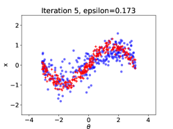
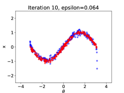
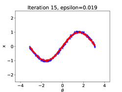
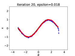
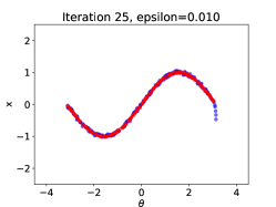
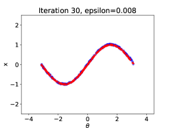
Figure 1: Sinusoidal example output. In each frame, dots are 300 samples from the current density $q$. Crosses are 300 samples targeting $p_{\epsilon}(\theta)$. These are based on the importance sampling stage of Algorithm 1 (steps 3–6) using $q$ as a proposal, with importance resampling (see Section 4.3) used to get unweighted samples.

7 Example: M/G/1 Queue

7.1 Model

Consider a M/G/1 queuing model of a single queue of customers. Times between arrivals at the back of the queue are $\text{Exp}(\theta_{1})$. On reaching the front of the queue, a customer’s service time is $U(\theta_{2},\theta_{3})$. All these random variables are independent. We consider a setting where only inter-departure times are observed: times between departures from the queue.

We sample a synthetic dataset of $20$ observations from parameter values $\theta_{1}=0.1,\theta_{2}=4,\theta_{3}=5$. We attempt to infer these parameters under the prior $\theta_{1}\sim U(0,1/3),\theta_{2}\sim U(0,10),\theta_{3}-\theta_{2}\sim U(0,10)$ (all independent).

7.2 Existing Methods

The M/G/1 model with inter-departure observations is a common benchmark for likelihood-free inference, which can often provide fast approximate inference. See Papamakarios et al., (2019) for a comparison of methods for an M/G/1 example. A potential disadvantage of existing likelihood-free methods is that they typically require using low dimensional summary statistics to be efficient, and this can lose some information from the data. As a likelihood-free inference baseline, we investigate a ABC-PMC algorithm. This is a modification of existing ABC-PMC methods to use the unnormalised target (6). See Section C of the supplement for full details.

We also include results from a sophisticated MCMC scheme (Shestopaloff and Neal,, 2014) for this model. This provides near-exact samples from the posterior, which is a useful gold standard comparison for the approximate inference methods. A limitation of this MCMC scheme is the difficulty in adapting it to other observation regimes – e.g. observing the queue length at various times (Pickands and Stine,, 1997) – which would be relatively easy for likelihood-free methods.

7.3 DIS Implementation

We introduce $\vartheta$ and $x$, vectors of length 3 and $2\dim(y)$, and take $\xi$ as the collection $(\vartheta,x)$. Our simulator transforms these inputs to $\theta(\vartheta)$ and $y(\xi)$, with the property that $\xi\sim\mathcal{N}(0,\mathrm{I})$ outputs a sample from the prior and the model. See the supplement (Section B) for details. We pretrain $q$ to approximate this distribution.

7.4 Results

Figure 2 (left) compares different choices of $N$ (number of importance samples) and $M$ (target ESS). It shows that $\epsilon$ reduces more quickly for smaller $M/N$ and smaller $N$, with $M/N$ having most influence. Note that small $N$ also has the advantage of lower memory requirements.

This tuning study suggests taking $N$ and $M/N$ as small as possible, while ensuring $M$ is at least a few hundred to avoid high variance in the importance sampling estimates. We use this guidance here and in the next section’s example. In both these examples, the cost of a single simulator run is low. For more expensive models efficient tuning choices may differ.

Figure 2 (right) is based on the DIS results with $N=5000$ and $M=250$, following by a final importance sampling step with $750,000$ samples, which takes a further 7.2 minutes. The results are a reasonably close match to near-exact MCMC output using the algorithm of Shestopaloff and Neal, (2014). The DIS results for $\theta_{2}$ and $\theta_{3}$ are more diffuse than the MCMC results. Also the $\theta_{2}$ DIS results lacks the sharp truncation of the right tail present in the MCMC results. (Truncation occurs at the minimum observed inter-departure time of $4.01$, as the minimum service time cannot be greater than this.)

We also compare DIS to our ABC-PMC baseline, under a similar runtime. For full details of methods and results see the supplement (Section C). Table 1 summarizes the results. ABC-PMC without summary statistics targets (6), just as DIS does, but cannot reach as low an $\epsilon$ value in the same time, so it produces inaccurate estimates for all parameters. To improve ABC-PMC performance, we consider replacing the data with summaries: quartiles of the inter-departure times, as used in Papamakarios et al., (2019). This improves results for $\theta_{1}$ and $\theta_{2}$, but still produces severe bias for $\theta_{3}$.

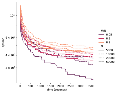
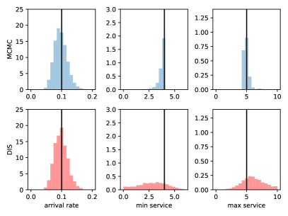
Figure 2: M/G/1 results. Left: The $\epsilon$ value reached by DIS on the M/G/1 example against computation time, for various choices of $N$ (number of importance samples) and $M/N$ (ratio of target effective sampling size to $N$). Right: Marginal posterior histograms for M/G/1 example. The DIS output shown is for $\epsilon=2.30$, which took 60 minutes to reach. To produce DIS histograms we ran a final stage of importance sampling with $750,000$ samples, and then used importance resampling (see Section 4.3) to get unweighted samples.

	$\theta_{1}$ (arrival rate)	$\theta_{2}$ (min service time)	$\theta_{3}$ (max service time)
MCMC	0.098 (0.060, 0.142)	3.72 (2.43, 4.00)	5.0 (4.4, 6.9)
ABC (no summaries)	0.147 (0.070, 0.303)	6.72 (2.15, 9.47)	19.0 (12.4, 26.1)
ABC (summaries)	0.094 (0.056, 0.128)	3.82 (2.92, 4.26)	9.0 (7.9, 11.3)
ABC (no summaries)	0.149 (0.066, 0.318)	6.20 (2.55, 9.63)	18.0 (10.6, 24.4)
ABC (summaries)	0.093 (0.056, 0.134)	3.80 (3.03, 4.33)	8.8 (7.6, 9.8)
DIS	0.098 (0.060, 0.145)	2.85 (0.20, 5.43)	6.4 (2.7, 11.1)

Table 1: Estimated posterior means and 95% quantile intervals for the M/G/1 example using various methods: MCMC (near-exact), ABC without summary statistics for $\epsilon=6.32$, ABC with quartile summaries for $\epsilon=0.16$, DIS for $\epsilon=2.30$. The $\epsilon$ values resulted from running ABC and DIS methods for roughly equal times.

8 Example: Susceptible-Infective Process on a Random Network

This section illustrates how DIS can be used to infer discrete variables. The key idea is to represent them as transformations of continuous latent variables. Such a mapping must be non-injective, and this is supported by the DIS algorithm without a need for any modifications.

We demonstrate this in the context of a spreading process model of an infectious disease on a random network, specifically a susceptible-infective (SI) compartmental model on a Erdős-Rényi network. See Dutta et al., (2018) for a discussion of similar models, although not the exact one we consider.

8.1 Model

Our model represents a population of $m$ individuals as a network. Each individual corresponds to a node. The individuals are labelled $0,1,\ldots,m-1$. An edge indicates contact between the corresponding individuals. The network is assumed to be an instance of the Erdős-Rényi random network (Erdős and Rényi,, 1959), so each pair of nodes form an edge with probability $\theta_{1}$.

The spreading process of the infectious disease is modelled as a discrete-time process. We consider a compartmental model where at any time each individual is in one of three states: susceptible, infective or immune. Initially there is a single infective node, individual 0. Susceptible neighbours of an infective individual at time $t$ are exposed and become infective at time $t+1$ with probability $\theta_{2}$. Exposed individuals who are not infected instead become immune. (All infection and edge formation events are assumed independent.)

Parameters $\theta_{1}$ and $\theta_{2}$ have independent $U(0,1)$ prior distributions. We assume that the observations are a binary vector indicating infective status for each node/time combination.

8.2 Likelihood-based Inference

The likelihood function of the model can be calculated by summing contributions from all possible networks, as detailed in the supplement (Section D). This is computationally feasible for small $m$, enabling near-exact posterior inference. Below, we use likelihood-based importance sampling as a benchmark for an example with $m=5$. However, likelihood calculations become infeasibly expensive for larger $m$, as the number of networks to sum is $2^{m(m-1)/2}$. For instance below we also investigate an example with $m=10$, giving $2^{45}\approx 3\times 10^{13}$ total networks.

8.3 DIS Implementation

Latent Variables and Simulator

Similarly to Section 7, we introduce vectors of latent variables $\vartheta,x_{\text{edge}},x_{\text{infect}}$. Here $\dim(\vartheta)=2,\dim(x_{\text{edge}})=\binom{m}{2},\dim(x_{\text{infect}})=m$. Now $\xi$ is the collection $(\vartheta,x_{\text{edge}},x_{\text{infect}})$.

Our simulator transforms these inputs to $\theta(\vartheta)$ and $y(\xi)$. As in Section 7, the simulator has the property that $\xi\sim\mathcal{N}(0,\mathrm{I})$ produces samples from the prior and model. We pretrain $q$ to approximate this distribution. Full details of the simulator transformation are in the supplement (Section D). In brief, $x_{\text{edge}}$ has an entry for each possible edge. An edge occurs when the corresponding entry falls below a threshold controlled by $\vartheta_{1}$. Similarly $x_{\text{infect}}$ has an entry for each individual. When that individual is exposed, then infection occurs if the corresponding entry falls below a threshold controlled by $\vartheta_{2}$. (Only one random variable is needed per individual as they can only be exposed once. Afterwards they are either infective or immune.)

To summarize, as well as continuous parameters $\theta$ we also wish to infer discrete variables: presence of edges and infection status. As noted at the start of Section 8, the discrete variables are inferred by representing them as a mapping of continuous latent variables $\xi$.

8.4 Results

We first consider a small network with $m=5$ nodes, observed for $5$ time steps. This has $\dim(\xi)=17$. Following Section 7 we use $N=5000$ and $M=250$ in DIS. As discussed in Section 3.2, it is plausible here for DIS to reach $\epsilon=0$, since the data are discrete. Our experiment reaches $\epsilon=0$ after 1.4 minutes. Then we perform importance sampling using this DIS proposal with $100,000$ samples, which takes a further 1.2 minutes. Figure 3 shows posterior histograms for $\theta$ match those for likelihood-based importance sampling, which produces $100,000$ samples in only 4 seconds.

Next we consider a larger network with $m=10$ nodes, observed for $10$ time steps. Now $\dim(\xi)=57$. As described in Section 8.2, exact likelihood calculation is infeasible here. However DIS with $N=5000$, $M=250$ can perform exact inference, reaching $\epsilon=0$ after 393 minutes. Figure 4 (left) shows the resulting posterior histograms for $\theta$. Then we perform importance sampling using this DIS proposal with $20,000$ samples, which takes a further 1.7 minutes.

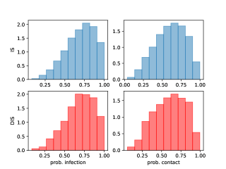
Figure 3: Output for SI example with $m=5$, showing marginal posterior histograms for parameters $\theta_{1}$ and $\theta_{2}$ from IS and DIS output. To produce DIS histograms we ran a final stage of importance sampling with $100,000$ samples and then used importance resampling (see Section 4.3) to get unweighted samples.

DIS also outputs posterior distributions of the latent variables $x_{\text{edge}}$ and $x_{\text{infect}}$, controlling the network structure and whether individuals become immune on exposure. These are summarized in Figure 4 (right). In the observed data, only individuals 1 and 7 do not become infected. The figure shows these individuals have a low posterior probability of becoming infected on exposure. Individual 0 has a moderate probability of infection on exposure. This is because they are already infective initially, so there is little information in the data on what would happen to them on exposure. The remaining individuals have a high posterior probability of becoming infected. In the data, individuals 3,6,8 are infected in the first time period. Consequently the edges from these to individual 0 have the highest posterior probabilities, as this is the only possible route of infection. Edges representing plausible routes to individuals infected later have lower probabilities, presumably as there are more possibilities for how this happens. The lowest probability edges are those which would result in individuals being infected before this is observed to happen in the data e.g. the edge $(0,2)$.

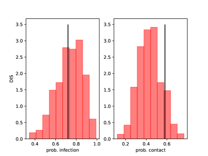
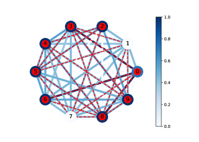
Figure 4: DIS output for SI example with $m=10$. To produce the plots we ran a final stage of importance sampling with $20,000$ samples, and then used importance resampling (see Section 4.3) to get unweighted samples. Left: Marginal posterior histograms for parameters $\theta_{1}$ and $\theta_{2}$. Vertical lines show the true values. Right: Posterior distribution of the network structure. Colours (in electronic version) / shades (in printed version) indicate the posterior probability of the existence of an edge and that a node will be infected upon exposure. Nodes represented by shaded circles are infective at some point, and dashed edges are those existing in the true network.

9 Conclusion

We present distilled importance sampling for likelihood-free inference, and show its application in several examples. An M/G/1 queuing example demonstrates that the method produces approximate results which are much more accurate than ABC, without needing the use of summary statistics. An epidemic model example shows that the method can also produce inference for discrete data. Indeed it demonstrates that for discrete data, it is possible for DIS to target the exact posterior. We also investigate tuning choices, and propose some default choices. The supplement (Section E) has a summary of tuning recommendations, and discussion of some alternative possibilities.

The remainder of the section discusses possible extensions of our methodology, as well as limitations.

Likelihood-Based Inference

This paper concentrates on likelihood-free inference. DIS can also be applied to some likelihood-based inference problems. However, exploratory work shows that here it perform less well than the competing methods listed at the start of Section 1.1. See the supplement (Section F) for further discussion.

More Efficient Training

Every iteration of Algorithm 1 generates new model simulations, and uses them for a few iterations of training. This results in a computationally feasible algorithm for our examples, as the simulators are reasonably fast. However for more expensive simulators, it would be desirable to use simulations more efficiently in the training process. For instance, training could continue with the same training data until convergence – although this risks overtraining. Alternatively, training data from all previous iterations could be reused for training – although ensuring the correct target distribution may be difficult. We plan to explore these approaches in future work.

Amortised Flows

Throughout the paper, $q(\xi;\phi)$ is a generic normalizing flow producing the vector $\xi$. We refer to this as a black-box approach, since it involves no knowledge of how $x$ is used by the simulator. This is less practical for large $\dim(\xi)$, as an increasingly large amount of simulations are required to learn such a high dimensional distribution.

An alternative is leveraging amortization in the flow, using knowledge about the simulator. Suppose a simulator requests a random variable. An amortized flow would determine the distribution to sample from using knowledge of: previously returned random variables (as for a black-box flow); the current simulator state; the line of code making the request. The complexity of the flow now depends on the number of sampling statements in the code, rather than the total number of samples made. This can be a big reduction in complexity when the simulator makes many iterations over a few sample statements. Similar ideas appear in inference networks (Le et al.,, 2017).

Overriding Random Number Generators

For the examples in this paper, we wrote custom simulator code which allowed $x$ values sampled from $q$ to be supplied as input. For large simulator codebases, it would be ideal to work with the original code, without needing to develop a custom version. Following Baydin et al., (2019), a possible approach is to override the random number generator that the code uses to instead provide $x$ values proposed by $q$.

Use with CDE

As mentioned in Sections 1 and 2.1, one approach to likelihood-free inference is conditional density estimation (CDE). Unlike DIS, this allows amortized inference: after training it can be used for inference of many different observed datasets. Future work could combine the methods: use CDE to produce an initial approximate posterior estimate, then refine further using DIS. This makes use of complementary advantages of the methods: CDE is amortized, while DIS relies less on summary statistics.

Acknowledgments

The authors gratefully acknowledge: Alex Shestopaloff for providing MCMC code for the M/G/1 model; Sammy Ragy for spotting several typos; Andrew Golightly, Chris Williams and anonymous referees for helpful suggestions. This work was supported by the EPSRC under grant EPSRC EP/V049127/1 (Dennis Prangle); and Italian Ministry of University and Research (MIUR) under grant 58523_DIPECC (Cecilia Viscardi).

Supplementary Material

Appendix A Truncating Importance Weights

Importance sampling estimates can have large or infinite variance if the proposal density $\lambda$ is a poor approximation to the target density $p$. The practical manifestation of this is a small number of importance weights being very large relative to the others. To reduce the variance, Ionides, (2008) introduced truncated importance sampling. This replaces each importance weight $w_{i}$ with $\tilde{w}_{i}=\min(w_{i},\omega)$ given some threshold $\omega$. The truncated weights are then used in estimates (3) or (4) (from the main paper). Truncating in this way typically reduces variance, at the price of increasing bias.

Gradient clipping (Pascanu et al.,, 2013) in stochastic gradient optimization operates by truncating large gradient estimates. It is common practice to prevent occasional large gradient estimates from destabilizing optimization. Truncating importance weights in Algorithm 1 (the DIS algorithm in the main paper) has a similar effect of reducing the variability of gradient estimates. A potential drawback of either method is that gradients lose the property of unbiasedness, which is theoretically required for convergence to an optimum of the objective. Pascanu et al., (2013) give heuristic arguments for good optimizer performance when using truncated gradients, and we make the following similar case for using truncated weights. Firstly, even after truncation, the gradient is likely to point in a direction increasing the objective. In our approach, it should still increase the $q$ density at $\xi^{(i)}$ values with large $w_{i}$ weights, which is desirable. Secondly, we expect there is a region near the optimum for $\phi$ where truncation is extremely rare, and therefore gradient estimates have very low bias once this region is reached. Finally, we also observe good empirical behaviour in our examples, showing that optimization with truncated weights can find good importance sampling proposals.

Note that we could use gradient clipping directly in Algorithm 1. We prefer truncating importance weights as there is an automated way to choose the threshold $\omega$, as follows. We select $\omega$ to reduce the maximum normalized importance weight, $\max_{i}\frac{\tilde{w}_{i}}{\sum_{i=1}^{N}\tilde{w}_{i}}$, to a prespecified value: throughout we use $0.1$. The required $\omega$ can easily be calculated e.g. by bisection. (Occasionally no such $\omega$ exists i.e. if most $w_{i}$s are zero. In this case we set $\omega$ to the smallest positive $w_{i}$.)

Appendix B M/G/1 Model

This section describes the M/G/1 queuing model, in particular how to simulate from it.

Recall that the parameters are $\theta_{1},\theta_{2},\theta_{3}$, with independent prior distributions $\theta_{1}\sim U(0,1/3),\theta_{2}\sim U(0,10),\theta_{3}-\theta_{2}\sim U(0,10)$. We introduce a reparameterized version of our parameters: $\vartheta_{1},\vartheta_{2},\vartheta_{3}$ with independent $\mathcal{N}(0,1)$ priors. Then we can take $\theta_{1}=\Phi(\vartheta_{1})/3$, $\theta_{2}=10\Phi(\vartheta_{2})$ and $\theta_{3}=\theta_{2}+10\Phi(\vartheta_{3})$, where $\Phi$ is the $\mathcal{N}(0,1)$ cumulative distribution function.

The model involves independent latent variables $x_{i}\sim\mathcal{N}(0,1)$ for $1\leq i\leq 2m$, where $m=\dim(y)$ is the number of observations. These generate

$$a_{i} =-\frac{1}{\theta_{1}}\log\Phi(x_{i}),$$ (inter-arrival times)

$$s_{i} =\theta_{2}+(\theta_{3}-\theta_{2})\Phi(x_{i+m}).$$ (service times)

Inter-departure times can be calculated through the following recursion (Lindley,, 1952)

$$d_{i} =s_{i}+\max(A_{i}-D_{i-1}),$$ (inter-departure times)

where $A_{i}=\sum_{j=1}^{i}a_{j}$ (arrival times) and $D_{i}=\sum_{j=1}^{i}d_{j}$ (departure times).

Numerical Stability

To avoid occasional numerical stability problems, our implementation replaces the inter-arrival times equation above with

$$a_{i}=\min\left\{10^{6},-\frac{1}{\theta_{1}}\log[\Phi(x_{i})+10^{-20}]\right\}.$$

We expect this to have negligible impact on the final results.

Appendix C ABC Analysis of M/G/1 Example

As a baseline comparison, we perform inference for the M/G/1 example using approximate Bayesian computation (ABC). The algorithm and results are detailed here.

C.1 Algorithm

We implement ABC using Algorithm B below, a modified version of the popular ABC-PMC approach (Toni et al.,, 2009; Sisson et al.,, 2009; Beaumont et al.,, 2009). These algorithms target

$$\tilde{p}_{\epsilon}(\theta)=\pi(\theta)\int\mathbbm{1}[||y(\xi)-y_{0}||\leq\epsilon]\pi(x)dx,$$

where $||\cdot||$ is the Euclidean norm, and $\pi(x)$ is the density of the $x$ variables used in the simulator. A novelty of Algorithm B is that it instead targets

$$\tilde{p}_{\epsilon}(\theta)=\pi(\theta)\int\exp\left[-\tfrac{1}{2\epsilon^{2}}||y(\xi)-y_{0}||^{2}\right]\pi(x)dx.$$

This is the $\theta$ marginal of the joint target used by DIS, equation (6) of the main paper.

Iteration $t$ of Algorithm B produces a weighted sample $(\theta^{t}_{i},w^{t}_{i})_{1\leq i\leq N}$. This targets $\tilde{p}_{\epsilon_{t}}(\theta)$ in the same way as importance sampling output. Over the course of the algorithm, the value of $\epsilon_{t}$ is reduced, and the number of simulated datasets required for an iteration tends to increase.

Algorithm B ABC-PMC

1:initialize $\epsilon_{1}=\infty$

2:for $t=1,2,\ldots$ do

3:     Let $i=0$ (number of acceptances).

4:     while $i<N$ do

5:         Sample $\theta^{*}$ from $\lambda_{t}(\theta)$, defined in (12).

6:         if $\pi(\theta^{*})>0$ then

7:              Sample $x^{*}$ from $\pi(x)$ and let $y^{*}=y(\theta^{*},x^{*})$.

8:              Let $d^{*}=||y^{*}-y_{0}||$.

9:              Let $\alpha=\exp[-\tfrac{1}{2\epsilon_{t}^{2}}{d^{*}}^{2}]$.

10:              With probability $\alpha$ accept: let $\theta^{t}_{i}=\theta^{*}$, $d^{t}_{i}=d^{*}$, $w^{t}_{i}=\pi(\theta^{*})/\lambda_{t}(\theta^{*})$ and increment $i$ by 1.

11:         end if

12:     end while

13:     Calculate $\epsilon_{t+1}$ (see below).

14:end for

Step 5 of Algorithm B samples from the density $\lambda_{t}(\theta)$, where

$$\lambda_{1}(\theta) =\pi(\theta)$$ (12a)

$$\lambda_{t}(\theta) =\frac{\sum_{i=1}^{N}w_{i}^{t-1}K_{t}(\theta|\theta_{i}^{t-1})}{\sum_{i=1}^{N}w_{i}^{t-1}} \text{for }t>1.$$ (12b)

In the first iteration $\lambda_{t}(\theta)$ is the prior. After this, a kernel density estimate is used based on the previous weighted sample. We follow Beaumont et al., (2009) in using

$$K_{t}(\theta|\theta^{t-1})=\varphi(\theta^{t-1},2\Sigma_{t-1}),$$

where $\varphi$ is the density of a normal distribution and $\Sigma_{t-1}$ is the empirical variance matrix of $(\theta_{i}^{t-1})_{1\leq i\leq N}$ calculated using weights $(w_{i}^{t-1})_{1\leq i\leq N}$

To implement step 13 of the algorithm, we select $\epsilon_{t+1}$ so that the acceptance probability of a typical member of the previous weighted sample is reduced by a prespecified factor $k$. Specifically, we define $\tilde{d}$ as the median of the $d^{t}_{i}$ values, and find $\epsilon_{t+1}$ by solving

$$\alpha(\tilde{d},\epsilon_{t+1}) =k\alpha(\tilde{d},\epsilon_{t}),\quad\text{where}$$

$$\alpha(d,\epsilon) =\exp[-\tfrac{1}{2\epsilon^{2}}d^{2}].$$

C.2 Results

We run Algorithm B on the M/G/1 example with $k=0.7$ and $N=250$. Runtime is checked every time step 2 is reached, and the algorithm terminates if this exceeds 70 minutes: the time used by DIS for this example in the main paper (including the final importance sampling stage).

Our implementation details give some modest advantages to ABC-PMC. Firstly, under our stopping rule, the final iteration of ABC-PMC typically continues several minutes beyond 70 minutes, providing it with more computational resources than DIS. Secondly, the ABC-PMC algorithm can perform more simulations per minute than DIS in this example. This is because later ABC-PMC iterations require large numbers (millions) of simulations, and our implementation was able to perform these in large parallel batches.

Despite these advantages, the final ABC-PMC $\epsilon$ value is $6.32$, which is much larger than the final value for DIS, $\epsilon=2.30$. Recall that the approximate posterior under $\epsilon$ is the exact posterior for data observed with independent Gaussian errors of scale $\epsilon$ (Wilkinson,, 2013). At $\epsilon=6.32$ this extra error is large compared to the data (whose values range from 4 to 34), hence it seems likely to produce significant approximation error. This is reflected in very wide posterior marginals – see Figure 5. Further, the asymptotic cost per output sample of ABC is $O(\epsilon^{-\dim(y)})$ (Prangle et al.,, 2018), suggesting that reaching $\epsilon=2.30$ using ABC requires a factor of $(2.30/6.32)^{-20}\approx 6.0\times 10^{8}$ more simulations, which is computationally infeasible.

To reduce the computational cost of ABC, the data are often replaced by low dimensional summary statistics. We investigate using quartiles of the inter-departure times as summaries, following Papamakarios and Murray, (2016). This is done by adding a final step to the simulator which converts the raw data to quartiles, and letting $y_{0}$ be the observed quartiles. We run ABC-PMC with quartile statistics using the same tuning details as above. The final $\epsilon$ value is now $0.16$. Figure 5 shows that the posterior marginals are much improved. However the maximum service time marginal is still a poor approximation of the near-exact MCMC results, suggesting that the summaries have lost information from the raw data.

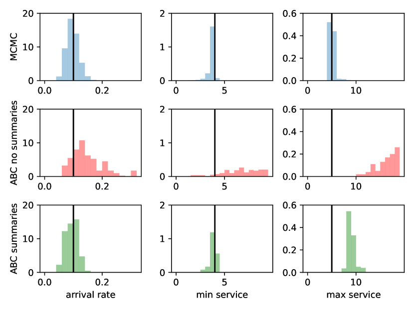
Figure 5: Marginal posterior histograms for M/G/1 example. Top: MCMC output. Middle: ABC output without summary statistics for $\epsilon=6.32$. Bottom: ABC output with quartile summaries for $\epsilon=0.16$. The ABC histograms are based on samples drawn from ABC-PMC output by importance resampling.

Appendix D SI Process Example Further Details

In this section, we describe further details of our analysis of a SI process on a network.

D.1 Simulator

In this model, the parameters $\theta_{1}$ and $\theta_{2}$ represent the probability of contact and the probability of infection. They are a priori uniformly distributed on the unit interval. Let $\vartheta_{1}$ and $\vartheta_{2}$ be two independent $\mathcal{N}(0,1)$ random variables. We then take $\theta_{1}=\Phi(\vartheta_{1})$ and $\theta_{2}=\Phi(\vartheta_{2})$ where, as earlier, $\Phi$ is the $\mathcal{N}(0,1)$ cumulative distribution function.

Recall that $m$ is the number of nodes in the network. The latent variables $x_{\text{infect},1},\ldots,x_{\text{infect},m}$ determine whether a node becomes infected or immune on its first exposure to infection. The $i$-th node is infected at the first time period when it has a link to an infective node if $\Phi(x_{\text{infect},i})<\theta_{2}$ (or equivalently $x_{\text{infect},i}<\vartheta_{2}$). The latent variables $x_{\text{edge},1},\ldots,x_{\text{edge},m(m-1)/2}$ control network creation: there are $m(m-1)/2$ possible edges and the $j$-th edge (according to some enumeration of edges) is added when $\Phi(x_{j})<\theta_{1}$ (or equivalently $x_{j}<\vartheta_{1}$).

Clearly when $\vartheta,x_{\text{edge}},x_{\text{infect}}$ have a $\mathcal{N}(0,\mathrm{I})$ distribution, then the simulator produces a sample from the prior and model.

D.2 Likelihood-based Analysis

Here we detail how the likelihood function for this model can be computed, and outline why this is only computationally feasible for small $m$.

Our observations are the $I_{t,j}$ binary variables assuming value $1$ if the $j$-th node is infective at time $t$ and $0$ otherwise. Here $j\in\{0,1,\ldots,m-1\}$ and $t\in\{0,1,2,\ldots,T-1\}$. Define $I_{t}=(I_{t,0},I_{t,1},\ldots,I_{t,m-1})$. We assume $I_{0}$ is fixed as $(1,0,0,\ldots,0)$. So initially only individual 0 is infected.

Let us denote by $\mathcal{G}$ the set of adjacency matrices of size $m\times m$ for Erdős-Rényi networks. The likelihood function is then

$$\!\!\!L(\theta) =\Pr(I_{1},\ldots,I_{T-1}|\theta,I_{0})$$

$$=\sum\limits_{G\in\mathcal{G}}\Pr(I_{1},\ldots,I_{T-1},G|\theta,I_{0})$$

$$=\sum\limits_{G\in\mathcal{G}}\!\Pr(G|\theta_{1})\!\Pr(I_{1},\ldots,I_{T-1}|G,\theta_{2},I_{0}),\!$$ (13)

where $\Pr(G|\theta_{1})=\theta_{1}^{D}(1-\theta_{1})^{\binom{m}{2}-D}$ with $D=\sum\limits_{i=1}^{m}\sum\limits_{j=i}^{m}G_{i,j}$, the degree of the network.

Let $A_{1}$ be the set of nodes neighbouring the seed node (individual 0). For $t\geq 2$, let $A_{t}=A(I_{t-1},I_{t-2})$ be the set $\{j:(\bar{I}_{t-2,t-1}G)_{j}>0\}\cap\{j:I_{t-1,j}=0\}$ where $\bar{I}_{t-2,t-1}=I_{t-1}\odot(1-I_{t-2})$. (Recall $\odot$ represents elementwise multiplication.) Thus $A_{t}$ is the set of nodes that could be infected at time $t$ i.e. those susceptible at time $t-1$ and connected to a node that became infective at time $t-1$. Then

$$\Pr(I_{1},\ldots,I_{T-1}|G,\theta_{2},I_{0})$$

$$=\prod\limits_{t=2}^{T-1}\Pr(I_{t}|I_{t-1},I_{t-2},\theta_{2},G)\Pr(I_{1}|I_{0},\theta_{2},G)$$

$$=\prod\limits_{t=2}^{T-1}\prod\limits_{j=0}^{m-1}\Pr(I_{t,j}|I_{t-1},I_{t-2},\theta_{2},G)\Pr(I_{1}|I_{0},\theta_{2},G)$$

$$=\prod\limits_{t=1}^{T-1}\prod\limits_{j\in A_{t}}\theta_{2}^{I_{t,j}}(1-\theta_{2})^{1-I_{t,j}}\prod\limits_{j\notin A_{t}}{\mathbbm{1}\{I_{t-1,j}=I_{t,j}\}}.$$

From (13) it follows that with a small number of nodes the likelihood evaluation has an affordable computational cost. However, the cost increases exponentially in $m$ because (13) involves a summation over $\mathcal{G}$ having cardinality $2^{m(m-1)/2}$.

Appendix E Tuning Recommendations

Here we summarize recommendations on tuning DIS which appear throughout the paper, and add some further comments.

E.1 Hyperparameters

For the M/G/1 and SI network examples we recommend using:

• $N=5000$ (importance sampling sample size)

• $M=250$ (target effective sample size)

• $n=100$ (training batch size)

• $B=\lceil M/n\rceil=3$ (number of batches)

The sinusoidal example is much simpler, and we expect a wide range of tuning choices to work well. In the paper we use $N=4000,M=2000$ to allow easy visualization.

In general we expect optimizing these hyperparameters for particular tasks is likely to be useful. In particular, this paper focuses on simulators which are computationally cheap to run. For more expensive models, the optimal tuning choices could be qualitatively different.

E.2 Normalizing Flow Architecture

For all our examples we use an autoregressive neural spline flow for $q(\xi;\phi)$ with 5 bins for each variable, and bounding box $[-10,10]$. The spline details are output by an autoregressive residual neural network (Nash and Durkan,, 2019) with 3 blocks, 20 hidden features and ReLU activation. We recommend this as a default choice of architecture. However we expect more complex and higher dimensional targets to require larger architectures e.g. with more layers and hidden units.

An indication that a larger architecture is needed in the DIS algorithm is that $\epsilon_{t}$ stops decreasing at some $\epsilon^{*}>0$. This can occur when no density $q(\xi;\phi)$ from the current architecture is a sufficiently good approximation of $p_{\epsilon^{*}}$. Therefore it becomes extremely unlikely for the target ESS value to be attained, which is required to reduce $\epsilon_{t}$ further.

In exploratory work we also investigated the real NVP (“Non-Volume Preserving”) normalizing flow (Dinh et al.,, 2016). We found this flow could be much faster to use than a spline flow (i.e. more iterations of Algorithm 1 can be run per unit time). However it sometimes produced numerical errors in the M/G/1 example, and struggled to approximate the target for low $\epsilon$ in the SI network example. We speculate that the latter issue is because this posterior requires a complex dependency structure – e.g. the presence of some contact edges rule out other edges – that is easier to capture using an autoregressive flow. Due to these issues, we recommend spline flows as a default choice.

E.3 Selecting $\epsilon$

The method outlined in the main paper to select $\epsilon$ is free of tuning parameters. However, alternative methods to select $\epsilon$ could be used, for instance by using variations on the standard effective sample size (see e.g. Elvira et al.,, 2022).

Appendix F Likelihood-based inference

Here we expand on comments from the main paper’s conclusion, Section 9, on applying DIS to likelihood-based inference. This is possible when a full data likelihood $L(\theta,x)$ is available given some latent variables $x$, but integration to $L(\theta)$ is infeasibly computationally expensive. In this case the unnormalised DIS target $\tilde{p}_{\epsilon}$ would be a tempered form of $\pi(\xi)L(\theta,x)$, for instance $\tilde{p}_{\epsilon}(\xi)=\pi(\xi)L(\theta,x)^{1-\epsilon}$ (taking $\epsilon_{0}=1$).

Earlier drafts of this paper included such applications to likelihood-based inference. A reviewer suggested investigating how useful tempering was. Exploratory work found it was often of little use: simply initialising $\epsilon_{0}=0$ in our algorithm produced good results. The resulting algorithm has little novelty over other work listed at the start of Section 1.1. Therefore we have concentrated on LFI applications, where initialising $\epsilon_{0}=0$ is generally not feasible as it would result in all importance sampling weights being zero (almost surely for continuous data, or with high probability for high dimensional discrete data).

Our exploratory findings about the poor performance of tempering for likelihood-based applications of DIS may not apply to other related methods. For instance, a reviewer commented that there is some similarity between DIS for likelihood-based inference and recent work of Surjanovic et al., (2022). This also uses a tempering scheme and estimates densities by minimising the inclusive Kullback-Leibler divergence (equation (8) from the main paper). Their work attains good empirical results. However its goal is to create an efficient parallel tempering MCMC scheme, rather than an importance sampling proposal as in DIS.

References

- Agapiou et al., (2017) Agapiou, S., Papaspiliopoulos, O., Sanz-Alonso, D., and Stuart, A. M. (2017). Importance sampling: Intrinsic dimension and computational cost. Statistical Science, 32(3):405–431.
- Arbel et al., (2021) Arbel, M., Matthews, A., and Doucet, A. (2021). Annealed flow transport Monte Carlo. In International Conference on Machine Learning, pages 318–330.
- Baydin et al., (2018) Baydin, A. G., Pearlmutter, B. A., Radul, A. A., and Siskind, J. M. (2018). Automatic differentiation in machine learning: a survey. Journal of Marchine Learning Research, 18:1–43.
- Baydin et al., (2019) Baydin, A. G., Shao, L., Bhimji, W., Heinrich, L., Naderiparizi, S., Munk, A., Liu, J., Gram-Hansen, B., Louppe, G., Meadows, L., Torr, P., Lee, V., Cranmer, K., Prabhat, and Wood, F. (2019). Efficient probabilistic inference in the quest for physics beyond the standard model. In Advances in Neural Information Processing Systems, volume 32.
- Beaumont et al., (2009) Beaumont, M. A., Cornuet, J.-M., Marin, J.-M., and Robert, C. P. (2009). Adaptive approximate Bayesian computation. Biometrika, 96(4):2025–2035.
- Bornschein and Bengio, (2014) Bornschein, J. and Bengio, Y. (2014). Reweighted wake-sleep. arXiv preprint arXiv:1406.2751.
- Chatterjee and Diaconis, (2018) Chatterjee, S. and Diaconis, P. (2018). The sample size required in importance sampling. The Annals of Applied Probability, 28(2):1099–1135.
- Cornuet et al., (2012) Cornuet, J.-M., Marin, J.-M., Mira, A., and Robert, C. P. (2012). Adaptive multiple importance sampling. Scandinavian Journal of Statistics, 39(4):798–812.
- Cotter et al., (2020) Cotter, S. L., Kevrekidis, I. G., and Russell, P. (2020). Transport map accelerated adaptive importance sampling, and application to inverse problems arising from multiscale stochastic reaction networks. SIAM/ASA Journal on Uncertainty Quantification, 8(4):1383–1413.
- Del Moral et al., (2012) Del Moral, P., Doucet, A., and Jasra, A. (2012). An adaptive sequential Monte Carlo method for approximate Bayesian computation. Statistics and Computing, 22(5):1009–1020.
- Dieng et al., (2017) Dieng, A. B., Tran, D., Ranganath, R., Paisley, J., and Blei, D. (2017). Variational inference via upper bound minimization. In Advances in Neural Information Processing Systems, volume 30.
- Dinh et al., (2016) Dinh, L., Sohl-Dickstein, J., and Bengio, S. (2016). Density estimation using real NVP. arXiv preprint arXiv:1605.08803.
- Duan, (2021) Duan, L. L. (2021). Transport Monte Carlo: high-accuracy posterior approximation via random transport. Journal of the American Statistical Association (online preview).
- Durkan et al., (2019) Durkan, C., Bekasov, A., Murray, I., and Papamakarios, G. (2019). Neural spline flows. In Advances in Neural Information Processing Systems, volume 32.
- Dutta et al., (2018) Dutta, R., Mira, A., and Onnela, J.-P. (2018). Bayesian inference of spreading processes on networks. Proceedings of the Royal Society A: Mathematical, Physical and Engineering Sciences, 474(2215):20180129.
- Elvira et al., (2022) Elvira, V., Martino, L., and Robert, C. P. (2022). Rethinking the effective sample size. International Statistical Review.
- Erdős and Rényi, (1959) Erdős, P. and Rényi, A. (1959). On random graphs. Publicationes Mathematicate, 6:290–297.
- Foerster et al., (2018) Foerster, J., Farquhar, G., Al-Shedivat, M., Rocktäschel, T., Xing, E., and Whiteson, S. (2018). Dice: The infinitely differentiable Monte Carlo estimator. In International Conference on Machine Learning, pages 1529–1538.
- Germain et al., (2015) Germain, M., Gregor, K., Murray, I., and Larochelle, H. (2015). MADE: Masked autoencoder for distribution estimation. In International Conference on Machine Learning, pages 881–889.
- Graham and Storkey, (2017) Graham, M. M. and Storkey, A. J. (2017). Asymptotically exact inference in differentiable generative models. Electronic Journal of Statistics, 11(2):5105–5164.
- Grazian and Fan, (2019) Grazian, C. and Fan, Y. (2019). A review of approximate Bayesian computation methods via density estimation: Inference for simulator-models. Wiley Interdisciplinary Reviews: Computational Statistics, 12(4):e1486.
- Huggins et al., (2020) Huggins, J. H., Kasprzak, M., Campbell, T., and Broderick, T. (2020). Practical posterior error bounds from variational objectives. In Artificial Intelligence and Statistics, pages 1792–1802.
- Ikonomov and Gutmann, (2020) Ikonomov, B. and Gutmann, M. U. (2020). Robust optimisation Monte Carlo. In International Conference on Artificial Intelligence and Statistics, pages 2819–2829.
- Ionides, (2008) Ionides, E. L. (2008). Truncated importance sampling. Journal of Computational and Graphical Statistics, 17(2):295–311.
- Jerfel et al., (2021) Jerfel, G., Wang, S., Fannjiang, C., Heller, K. A., Ma, Y., and Jordan, M. I. (2021). Variational refinement for importance sampling using the forward Kullback-Leibler divergence. In Uncertainty in Artificial Intelligence, pages 1819–1829.
- Kingma and Ba, (2015) Kingma, D. P. and Ba, J. (2015). Adam: A method for stochastic optimization. In International Conference on Learning Representations.
- Larrañaga and Lozano, (2002) Larrañaga, P. and Lozano, J. A. (2002). Estimation of distribution algorithms: A new tool for evolutionary computation. Springer.
- Le et al., (2017) Le, T. A., Baydin, A. G., and Wood, F. (2017). Inference compilation and universal probabilistic programming. In Artificial Intelligence and Statistics, pages 1338–1348.
- Li et al., (2017) Li, Y., Turner, R. E., and Liu, Q. (2017). Approximate inference with amortised MCMC. arXiv preprint arXiv:1702.08343.
- Lindley, (1952) Lindley, D. V. (1952). The theory of queues with a single server. Mathematical Proceedings of the Cambridge Philosophical Society, 48(2):277–289.
- Liu, (1996) Liu, J. S. (1996). Metropolized independent sampling with comparisons to rejection sampling and importance sampling. Statistics and Computing, 6(2):113–119.
- MacKay, (2003) MacKay, D. J. C. (2003). Information theory, inference and learning algorithms. Cambridge University Press.
- Marin et al., (2012) Marin, J.-M., Pudlo, P., Robert, C. P., and Ryder, R. J. (2012). Approximate Bayesian computational methods. Statistics and Computing, 22(6):1167–1180.
- Meeds and Welling, (2015) Meeds, T. and Welling, M. (2015). Optimization Monte Carlo: Efficient and embarrassingly parallel likelihood-free inference. Advances in Neural Information Processing Systems, 28.
- Mohamed et al., (2020) Mohamed, S., Rosca, M., Figurnov, M., and Mnih, A. (2020). Monte Carlo gradient estimation in machine learning. Journal of Machine Learning Research, 21(132):1–62.
- Müller et al., (2019) Müller, T., Mcwilliams, B., Rousselle, F., Gross, M., and Novák, J. (2019). Neural importance sampling. ACM Transactions on Graphics (TOG), 38(5):1–19.
- Naesseth et al., (2021) Naesseth, C. A., Lindsten, F., and Blei, D. (2021). Markovian score climbing: Variational inference with . In Advances in Neural Information Processing Systems, volume 33, pages 15499–15510.
- Nash and Durkan, (2019) Nash, C. and Durkan, C. (2019). Autoregressive energy machines. In International Conference on Machine Learning, pages 1735–1744.
- Papamakarios and Murray, (2016) Papamakarios, G. and Murray, I. (2016). Fast -free inference of simulation models with Bayesian conditional density estimation. In Advances in Neural Information Processing Systems, volume 29.
- Papamakarios et al., (2021) Papamakarios, G., Nalisnick, E., Rezende, D. J., Mohamed, S., and Lakshminarayanan, B. (2021). Normalizing flows for probabilistic modeling and inference. Journal of Machine Learning Research, 22(57):1–64.
- Papamakarios et al., (2019) Papamakarios, G., Sterratt, D., and Murray, I. (2019). Sequential neural likelihood: Fast likelihood-free inference with autoregressive flows. In Artificial Intelligence and Statistics, pages 837–848.
- Pascanu et al., (2013) Pascanu, R., Mikolov, T., and Bengio, Y. (2013). On the difficulty of training recurrent neural networks. In International Conference on Machine Learning, pages 1310–1318.
- Paszke et al., (2019) Paszke, A., Gross, S., Massa, F., Lerer, A., Bradbury, J., Chanan, G., Killeen, T., Lin, Z., Gimelshein, N., Antiga, L., et al. (2019). Pytorch: An imperative style, high-performance deep learning library. In Advances in Neural Information Processing Systems, volume 32.
- Pickands and Stine, (1997) Pickands, III, J. and Stine, R. A. (1997). Estimation for an M/G/ queue with incomplete information. Biometrika, 84(2):295–308.
- Prangle et al., (2018) Prangle, D., Everitt, R. G., and Kypraios, T. (2018). A rare event approach to high-dimensional approximate Bayesian computation. Statistics and Computing, 28(4):819–834.
- Robert and Casella, (2013) Robert, C. P. and Casella, G. (2013). Monte Carlo statistical methods. Springer.
- Rubinstein, (1999) Rubinstein, R. (1999). The cross-entropy method for combinatorial and continuous optimization. Methodology and computing in applied probability, 1(2):127–190.
- Rubinstein and Kroese, (2016) Rubinstein, R. Y. and Kroese, D. P. (2016). Simulation and the Monte Carlo method. John Wiley & Sons.
- Ruder, (2016) Ruder, S. (2016). An overview of gradient descent optimization algorithms. arXiv preprint arXiv:1609.04747.
- Shestopaloff and Neal, (2014) Shestopaloff, A. Y. and Neal, R. M. (2014). On Bayesian inference for the M/G/1 queue with efficient MCMC sampling. arXiv preprint arXiv:1401.5548.
- Sisson et al., (2009) Sisson, S. A., Fan, Y., and Tanaka, M. M. (2009). Correction: Sequential Monte Carlo without likelihoods. Proceedings of the National Academy of Sciences, 106(39):16889–16890.
- Smith and Gelfand, (1992) Smith, A. F. M. and Gelfand, A. E. (1992). Bayesian statistics without tears: a sampling–resampling perspective. The American Statistician, 46(2):84–88.
- Surjanovic et al., (2022) Surjanovic, N., Syed, S., Bouchard-Côté, A., and Campbell, T. (2022). Parallel tempering with a variational reference. arXiv preprint arXiv:2206.00080.
- Toni et al., (2009) Toni, T., Welch, D., Strelkowa, N., Ipsen, A., and Stumpf, M. (2009). Approximate Bayesian computation scheme for parameter inference and model selection in dynamical systems. Journal of The Royal Society Interface, 6(31):187–202.
- Wilkinson, (2013) Wilkinson, R. D. (2013). Approximate Bayesian computation (ABC) gives exact results under the assumption of model error. Statistical applications in genetics and molecular biology, 12(2):129–141.
- Yao et al., (2018) Yao, Y., Vehtari, A., Simpson, D., and Gelman, A. (2018). Yes, but did it work?: Evaluating variational inference. In International Conference on Machine Learning, pages 5581–5590.