Inhomogeneous chiral condensates in three-flavor quark matter

Abstract

We investigate the effect of strange-quark degrees of freedom on the formation of inhomogeneous chiral condensates in a three-flavor Nambu–Jona-Lasinio model in mean-field approximation. A Ginzburg-Landau study complemented by a stability analysis allows us to determine in a general way the location of the critical and Lifshitz points, together with the phase boundary where the (partially) chirally restored phase becomes unstable against developing inhomogeneities, without resorting to specific assumptions on the shape of the chiral condensate. We discuss the resulting phase structure and study the influence of the bare strange-quark mass $m_{s}$ and the axial anomaly on the size and location of the inhomogeneous phase compared to the first-order transition associated with homogeneous matter. We find that, as a consequence of the axial anomaly, critical and Lifshitz point split. For realistic strange-quark masses the effect is however very small and becomes sizeable only for small values of $m_{s}$.

I Introduction

Mapping the phase diagram of QCD at nonvanishing temperature $T$ and quark chemical potential $\mu$ is one of the major goals in strong interaction physics Kumar (2013); et al.(2011) (ed.). Lattice-QCD calculations revealed that chiral symmetry, which is spontaneously broken in vacuum, gets approximately restored at high temperature via a smooth crossover transition Aoki et al. (2006). At low temperature but nonvanishing chemical potential, standard lattice Monte-Carlo techniques are not applicable. In this regime one therefore has to rely on other approaches to QCD, like Dyson-Schwinger equations Fischer (2019) or the Functional Renormalization Group (FRG) Fu et al. (2019), or on effective models, like the Nambu–Jona-Lasinio (NJL) or the quark-meson model. Assuming spatially uniform chiral condensates, these approaches typically predict a first-order phase transition from the chirally broken to the (approximately) restored phase, ending at a critical end point Fischer (2019); Fu et al. (2019); Asakawa and Yazaki (1989); Scavenius et al. (2001). In the two-flavor chiral limit one finds instead a tricritical point where the first-order phase boundary at low $T$ is joined to a second-order one which replaces the crossover in the high-$T$–low-$\mu$ region. For simplicity we will refer to both the tricritical point and the critical end point as ‘critical point’ (CP) in the following.

Some time ago it was found that spatially inhomogeneous condensates could be favored over homogeneous ones in certain regions of the phase diagram Kutschera et al. (1990); Nakano and Tatsumi (2005); Nickel (2009a, b), see Ref. Buballa and Carignano (2015) for a review. In the chiral limit one then finds a so-called Lifshitz point (LP) where three phases, the homogeneous chirally broken phase, the restored phase and the inhomogeneous phase, meet. In particular it was found for the two-flavor NJL model in mean-field approximation that the inhomogeneous phase completely covers the first-order phase boundary between the homogeneous phases Nickel (2009b) and that the LP exactly coincides with the CP Nickel (2009a). Recently we have generalized this result to the case away from the chiral limit Buballa and Carignano (2019a). A similar picture also emerged from a truncated Dyson-Schwinger approach to QCD, although the coincidence of CP and LP has not yet been shown rigorously Müller et al. (2013). Indications for the presence of an inhomogeneous phase have also been found in a very recent FRG study of the QCD phase diagram Fu et al. (2019).

In the present article we want to investigate the effect of strangeness degrees of freedom on the locations of the CP and the LP in the NJL model. To this end we will employ the three-flavor NJL model and perform a Ginzburg-Landau (GL) analysis. In order to get a better feeling on the form of the phase diagram, this GL study will be supplemented by a stability analysis which, under certain conditions, can provide us the location of the phase boundary between the inhomogeneous and the partially chirally restored phase.

Our motivation for this study is twofold: First, in the two-flavor model the CP and the LP are typically found in a temperature and density regime where strange-quark effects may not be negligible. Including strangeness degrees of freedom will thus be a step toward a more realistic description. A first study of inhomogeneous phases in three-flavor matter has been performed in Ref. Moreira et al. (2014), albeit only for vanishing temperature and employing a simple explicit ansatz for the spatial dependence of the chiral condensate. The authors found that the coupling of strange and non-strange quarks, which is related to the axial anomaly, enlarges the inhomogeneous domain. Our investigation will be complementary, as its range of validity will be close to the locations of the CP and the LP at non-vanishing temperature, as well as along the phase boundary between the inhomogeneous and the partially restored phase. Moreover, it does not rely on a certain ansatz for the inhomogeneity and allows for a more transparent analysis of the role of the axial anomaly.

Our second motivation is the fact that QCD with three very light quark flavors is expected to have a first-order chiral phase transition even at $\mu=0$ Pisarski and Wilczek (1984). Hence if in three-flavor QCD the LP coincided with the CP, as it does in the two-flavor NJL model, it would mean that the inhomogeneous phase would also reach down to $\mu=0$ for small enough quark masses. At least in principle it could then be studied on the lattice in this case. As a first step we therefore want to investigate the behavior of CP and LP in the three-flavor NJL model. While it has been known for a long time that the CP indeed moves to lower chemical potentials when lowering the quark masses and eventually reaches the $T$ axis Fukushima (2008), until recently the behavior of the LP has not yet been studied for the three-flavor case. In particular it has not been checked whether CP and LP still coincide in that case.

Our paper is organized as follows. In Sect. II we introduce the three-flavor NJL model and derive a general expression for the mean-field thermodynamic potential as functional of several strange and non-strange chiral condensates with arbitrary spatial dependence. Based on this we perform in Sect. III a GL and a stability analysis, focusing on the locations of the CP and the LP as well as the position of the phase transition to the partially restored phase. In Sect. IV we give a quantitative illustration of the results by numerical evaluation of the GL coefficients before we draw our conclusions in Sect. V.

II NJL model setup

Our starting point is the three-flavor NJL Lagrangian

$$\mathcal{L}=\bar{\psi}\left(i\gamma^{\mu}\partial_{\mu}-\hat{m}\right)\psi+\mathcal{L}_{4}+\mathcal{L}_{6}$$ (1)

where $\psi=(u,d,s)^{T}$ denotes a quark field with three flavor degrees of freedom and $\hat{m}$ is the matrix containing their current masses. The last two terms describe a $U(3)_{L}\times U(3)_{R}$ invariant four-point interaction

$$\mathcal{L}_{4}=G\sum_{a=0}^{8}\left[(\bar{\psi}\tau_{a}\psi)^{2}+(\bar{\psi}i\gamma_{5}\tau_{a}\psi)^{2}\right],$$ (2)

and a six-point (“Kobayashi - Maskawa - ’t Hooft”, KMT) interaction

$$\mathcal{L}_{6}=-K\left[\mathrm{det}_{f}\bar{\psi}(1+\gamma_{5})\psi+\mathrm{det}_{f}\bar{\psi}(1-\gamma_{5})\psi\right]\,,$$ (3)

which is $SU(3)_{L}\times SU(3)_{R}$ symmetric but breaks the $U(1)_{A}$ symmetry, thus mimicking the axial anomaly. In the former $\tau_{a}$, $a=1,\dots,8$, denote Gell-Mann matrices in flavor space while $\tau_{0}=\sqrt{2/3}\,\mathbb{1}$ is proportional to the unit matrix.

Following standard procedures, we perform a mean-field approximation, considering scalar and pseudoscalar flavor-diagonal condensates,

$$\sigma_{f}({\bf x})\equiv{\langle{\bar{f}f}\rangle}({\bf x})\,,\qquad\pi_{f}({\bf x})\equiv{\langle{\bar{f}\,i\gamma^{5}f}\rangle}({\bf x})\,,\qquad f=\{u,d,s\}\,,$$ (4)

allowing them to be spatially dependent. The mean-field quark self-energies can then be expressed in terms of the mass operators

$${\hat{M}}_{f}({\bf x})=m_{f}-4G\sigma_{f}({\bf x})+2K\Big{(}\sigma_{g}({\bf x})\sigma_{h}({\bf x})-\pi_{g}({\bf x})\pi_{h}({\bf x})\Big{)}+i\gamma^{5}\Big{[}-4G\pi_{f}({\bf x})-2K(\sigma_{g}({\bf x})\pi_{h}({\bf x})+\pi_{g}({\bf x})\sigma_{h}({\bf x}))\Big{]}\,,$$ (5)

where $f\neq g\neq h\neq f$. We furthermore assume isospin symmetry in the light sector, $m_{u}=m_{d}\equiv m_{\ell}$, and thus

$$\sigma_{u}({\bf x})=\sigma_{d}({\bf x})\equiv\sigma_{\ell}({\bf x})$$ (6)

due to the flavor symmetry of the interaction. For the pseudoscalar condensates, given the isospin structure in the light sector, we identify

$$\pi_{u}({\bf x})=-\pi_{d}({\bf x})\equiv\pi_{\ell}({\bf x}),$$ (7)

while we neglect the pseudoscalar condensate in the strange sector, $\pi_{s}=0$. The latter is motivated by the fact that pseudoscalar condensates are usually suppressed by the presence of non-vanishing bare quark masses, which we will always consider in the strange sector.

The mass operators then reduce to

$${\hat{M}}_{u}({\bf x}) =m_{\ell}-\left[4G-2K\sigma_{s}({\bf x})\right]\left(\sigma_{\ell}({\bf x})+i\gamma^{5}\pi_{\ell}({\bf x})\right)\,,$$

$${\hat{M}}_{d}({\bf x}) =m_{\ell}-\left[4G-2K\sigma_{s}({\bf x})\right]\left(\sigma_{\ell}({\bf x})-i\gamma^{5}\pi_{\ell}({\bf x})\right)\,,$$

$${\hat{M}}_{s}({\bf x}) =m_{s}-4G\sigma_{s}({\bf x})+2K\left(\sigma_{\ell}^{2}({\bf x})+\pi_{\ell}^{2}({\bf x})\right)\,,$$ (8)

which is a considerable simplification compared to Eq. (5) but still catches the most important structures. For instance, it is compatible with the ansatz of Ref. Moreira et al. (2014), which we will briefly discuss at the end of this section.

Neglecting fluctuations, the mean-field thermodynamic potential at temperature $T$ and quark chemical potential $\mu$ is then given by

$$\Omega(T,\mu)=-\frac{T}{V}\,\mathbf{Tr}\,\log\frac{S^{-1}}{{T}}\,+\,\frac{1}{V}\int\limits_{V}d^{3}x\,\Big{\{}2G\big{[}2(\sigma_{\ell}^{2}+\pi_{\ell}^{2})+\sigma_{s}^{2}\big{]}-4K(\sigma_{\ell}^{2}+\pi_{\ell}^{2})\sigma_{s}\Big{\}}\,,$$ (9)

where $V$ is a quantization volume and $\mathbf{Tr}$ denotes a functional trace to be taken in the Euclidean space-time ($(it,{\bf x})\in V_{4}=[0,\frac{1}{T}]\times V$) and over internal (Dirac, color, and flavor) degrees of freedom. The inverse dressed quark propagator is given by $S^{-1}=\mathrm{diag}_{f}(S^{-1}_{u},S^{-1}_{d},S^{-1}_{s})$ with the flavor components

$$S^{-1}_{f}(x)=i\gamma^{\mu}\partial_{\mu}+\mu\gamma^{0}-{\hat{M}}_{f}(\mathbf{x})\,.$$ (10)

From the above expressions we can see that the different flavors only couple through the six-point interaction and thus for $K=0$ we obtain the usual expression for the two-flavor model plus a decoupled s-quark.

Having set up the model, we can now analyze its phase structure by minimizing $\Omega(T,\mu)$ with respect to the condensates. When restricting the analysis to homogeneous condensates, this is straightforward and has been done many times in the literature, see, e.g., Ref. Buballa (2005). With realistic parameters one basically obtains the result already mentioned in the Introduction, i.e., a first-order phase transition at low temperatures turning into a crossover at higher $T$, both of which can mainly be associated with the chiral restoration in the light-flavor sector. Further outside, i.e., at larger values of $\mu$ or $T$, there is another transition (usually a crossover) related to the partial symmetry restoration in the strange-quark sector. Although of minor importance for our GL analysis, this second transition will play a role for the behavior of the inhomogeneous phase at higher chemical potentials, as we will briefly discuss at the end of section IV.

The numerical analysis of the model phase diagram allowing for inhomogeneous condensates is obviously much more challenging, as one should in principle allow for arbitrary spatial modulations of $\sigma_{\ell}$, $\pi_{\ell}$, and $\sigma_{s}$. The authors of Ref. Moreira et al. (2014) have therefore restricted themselves to a relatively simple ansatz, namely a chiral density wave in the light sector, $\sigma_{\ell}({\bf x})=\sigma_{0}\cos({\bf q}\cdot{\bf x})$, $\pi_{\ell}({\bf x})=\sigma_{0}\sin({\bf q}\cdot{\bf x})$, $m_{\ell}=0$, embedded into a homogeneous strange-quark background $\sigma_{s}=\mathit{const.}$ Inserting this into Eq. (8), one finds that $\hat{M}_{s}=m_{s}-4G\sigma_{s}+2K\sigma_{0}^{2}$ is homogeneous as well, while $\hat{M}_{u}$ and $\hat{M}_{d}$ form an isospin doublet $\hat{M}_{\ell}=M_{0}\exp(i\gamma^{5}\tau^{3}{\bf q}\cdot{\bf x})$ with amplitude $M_{0}=-(4G-2K\sigma_{s})\sigma_{0}$. This feature allowed the authors to find the eigenvalue spectrum of the corresponding Hamiltonian by adopting the known two-flavor result Dautry and Nyman (1979). It should be noted, however, that this straightforward generalization of a known two-flavor solution was only possible because the space dependence of the $\sigma_{\ell}$ and $\pi_{\ell}$ contributions to $\hat{M}_{s}$ cancel each other for this ansatz. In contrast, the purely scalar “real-kink crystal”, which in the two-flavor model is energetically favored over the chiral density wave Nickel (2009b), cannot selfconsistently be generalized in this simple way since coupling it to a homogeneous $\sigma_{s}$ would still lead to an oscillating $\hat{M}_{s}$ as long as $K$ is nonzero.

In the remainder of this work we will not resort to a particular ansatz for the condensates but consider general functions $\sigma_{\ell}({\bf x})$, $\pi_{\ell}({\bf x})$, and $\sigma_{s}({\bf x})$ both within a GL as well as a stability analysis of the homogeneous phase. This will allow us, under certain conditions, to locate the position of the Lifshitz point together with the critical point and the phase boundary where inhomogeneous condensates become energetically favored.

III Ginzburg-Landau and stability analysis

The GL expansion of the thermodynamic potential allows for a systematic study of the phase structure while requiring only a limited number of assumptions. Generally, it corresponds to an expansion of the free energy in terms of one or more order parameters and their gradients, assuming that these quantities are small. In the context of chiral symmetry breaking the order parameter is usually identified with the chiral condensate, and the expansion is performed about the chirally restored solution where the condensate vanishes. Of course, this only works in the chiral limit, while in the presence of nonzero bare quark masses there is no chirally restored solution and therefore the expansion has to be performed around nonvanishing condensate values Buballa and Carignano (2019a).

On the other hand, in a realistic calculation the bare strange-quark mass is much larger than the bare masses of the up and down quarks. We may therefore study a partially simplified problem where we take into account $m_{s}\neq 0$ but consider $m_{\ell}=0$. In this case a two-flavor restored solution $\sigma_{\ell}=\pi_{\ell}=0$ exists, which we take as the expansion point of the GL analysis. In the strange-quark sector we proceed similarly as in Buballa and Carignano (2019a) for the case of light quarks away from the chiral limit and expand around a $T$ and $\mu$-dependent but spatially constant condensate $\sigma_{s}^{(0)}$, corresponding to a stationary point of $\Omega$ at $\sigma_{\ell}=\pi_{\ell}=0$. To this end we write

$$\sigma_{s}({\bf x})=\sigma_{s}^{(0)}+\delta\sigma_{s}({\bf x})$$ (11)

and introduce the order parameters

$$\Delta_{\ell}({\bf x})=-4G\left(\sigma_{\ell}({\bf x})+i\pi_{\ell}({\bf x})\right)\quad\text{and}\quad\Delta_{s}({\bf x})=-4G\,\delta\sigma_{s}({\bf x})\,,$$ (12)

which are proportional to the fluctuations around our expansion point and have the dimension of a mass. We then write

$$\Omega[\sigma_{\ell},\pi_{\ell},\sigma_{s}]=\Omega[0,0,\sigma_{s}^{(0)}]+\frac{1}{V}\int d^{3}x\,\omega_{GL}(\Delta_{\ell},\Delta_{s})\,,$$ (13)

and expand $\omega_{GL}$ in powers of $\Delta_{\ell}$ and $\Delta_{s}$ and gradients thereof.

Note that in Eq. (12) we combined the light-quark scalar and pseudoscalar condensates to a complex order parameter. In fact, as a consequence of the remaining two-flavor chiral symmetry, $\sigma_{\ell}$ and $\pi_{\ell}$ can be rotated into each other by a symmetry transformation and therefore $\omega_{GL}$ can only depend on the modulus of $\Delta_{\ell}$ but not on its phase. Moreover, since we expand about the two-flavor restored phase, only even powers of $|\Delta_{\ell}|$ are allowed. For $\Delta_{s}$, on the other hand, we can also have odd terms. Finally, the possible gradient terms are restricted by the requirement that the potential must be a scalar under spatial rotations.

Treating initially both light and strange order parameters as well as gradients to be of the same order, the GL functional up to order 4 thus takes the form

$$\omega_{GL}(\Delta_{\ell},\Delta_{s})=\phantom{+} \alpha_{2}|\Delta_{\ell}|^{2}+\alpha_{4,a}|\Delta_{\ell}|^{4}+\alpha_{4,b}|\nabla\Delta_{\ell}|^{2}+\dots$$

$$+ \beta_{1}\Delta_{s}+\beta_{2}\Delta_{s}^{2}+\beta_{3}\Delta_{s}^{3}+\beta_{4,a}\Delta_{s}^{4}+\beta_{4,b}(\nabla\Delta_{s})^{2}+\dots$$

$$+ \gamma_{3}|\Delta_{\ell}|^{2}\Delta_{s}+\gamma_{4}|\Delta_{\ell}|^{2}\Delta_{s}^{2}+\dots\,,$$ (14)

where the $\alpha$- and $\beta$-terms correspond to the contributions from the light and strange condensates, respectively, and the $\gamma$ terms describe the mixing.

Since we are expanding about a homogeneous stationary point, the linear coefficient $\beta_{1}$ associated with $\Delta_{s}$ has to vanish,

$$\left.\frac{\partial\omega_{GL}}{\partial\Delta_{s}}\right|_{\Delta_{\ell}=\Delta_{s}=0}=\beta_{1}=0\,.$$ (15)

This condition is of course equivalent to a gap equation for $\sigma_{s}^{(0)}$ at given $T$ and $\mu$.

For vanishing $\gamma_{i}$ the GL analysis of the non-strange sector would be identical to the two-flavor case in the chiral limit, which has been analyzed in Ref. Nickel (2009a). More specifically, the location of the CP, where the first-order phase transition turns into a second-order one, is given by the point where both the quadratic and quartic coefficients $\alpha_{2}$ and $\alpha_{4,a}$ vanish, while the LP appears where both $\alpha_{2}$ and the lowest-order gradient coefficient $\alpha_{4,b}$ become zero. For the standard two-flavor NJL model one finds that $\alpha_{4,a}=\alpha_{4,b}$ and as a consequence the CP and the LP coincide Nickel (2009a).

In order to study how these relations get modified in the presence of a third flavor coupled to the light sector, as reflected by $\gamma_{i}\neq 0$, the first step is to eliminate $\Delta_{s}$ by extremizing the thermodynamic potential with respect to this function. To this end we employ the Euler-Lagrange equations,

$$\frac{\partial\omega_{GL}}{\partial\Delta_{s}}-\partial_{i}\frac{\partial\omega_{GL}}{\partial\partial_{i}\Delta_{s}}=0\,,$$ (16)

which, after using the gap equation $\beta_{1}=0$, yields

$$\Delta_{s}=-\frac{\gamma_{3}}{2\beta_{2}}|\Delta_{\ell}|^{2}+\mathcal{O}(\Delta_{\ell}^{4})\equiv\Delta_{s}^{\mathit{extr}}\,.$$ (17)

Here, the orders in $\Delta_{\ell}$ and gradients are treated equally, $\mathcal{O}(\nabla^{n})=\mathcal{O}(\Delta_{\ell}^{n})$, as we already did when we wrote down Eq. (14). From Eq. (17) we then see, however, that $\Delta_{s}$ is of the order $\mathcal{O}(\Delta_{\ell}^{2})$. Inserting Eq. (17) back into Eq. (14) and keeping only terms up to the order $\mathcal{O}(\Delta_{\ell}^{4})$, one then obtains

$$\omega_{GL}(\Delta_{\ell},\Delta_{s}^{\mathit{extr}})=\alpha_{2}|\Delta_{\ell}|^{2}+\left(\alpha_{4,a}-\frac{\gamma_{3}^{2}}{4\beta_{2}}\right)|\Delta_{\ell}|^{4}+\alpha_{4,b}|\nabla\Delta_{\ell}|^{2}+\dots$$ (18)

We thus find that the quartic term in $\Delta_{\ell}$ gets an additional contribution through the coupling to the strange quarks, while the gradient term does not. So the relevant equations for locating the CP and the LP become

$$\alpha_{2}=0\;\;\text{and}\;\;\alpha_{4,CP}\equiv\alpha_{4,a}-\frac{\gamma_{3}^{2}}{4\beta_{2}}=0\quad\text{at the CP,}\qquad\alpha_{2}=0\;\;\text{and}\;\;\alpha_{4,LP}\equiv\alpha_{4,b}=0\quad\text{at the LP}\,,$$ (19)

and therefore, even if $\alpha_{4,a}$ and $\alpha_{4,b}$ were still equal (as they are in the two-flavor model) the CP and the LP would no longer coincide for $\gamma_{3}\neq 0$.

III.1 GL coefficients

In order to make more quantitative statements on the relative position of CP and LP, we need to determine the GL coefficients explicitly. To this end we basically follow the procedure of Ref. Nickel (2009a), although the present case is technically somewhat more involved due to the nonvanishing strange-quark mass and the presence of the KMT term.

In a first step we decompose the mass operator for flavor $f$ into a constant and a fluctuating piece,

$$\hat{M}_{f}({\bf x})=M_{f,0}+\delta\hat{M}_{f}({\bf x})\,,$$ (20)

by inserting Eqs. (11) and (12) into Eq. (8). Explicitly one finds

$$M_{s,0}=m_{s}-4G\sigma_{s}^{(0)}\,,\quad \delta\hat{M}_{s}({\bf x})=\Delta_{s}({\bf x})+{\kappa}|\Delta_{\ell}|^{2}\,,$$ (21)

$$M_{u,0}=M_{d,0}=0\,,\quad \delta\hat{M}_{u\atop d}({\bf x})=\left[1+{\delta+\kappa}\Delta_{s}({\bf x})\right]\left(\mathrm{Re}\Delta_{\ell}({\bf x})\pm i\gamma^{5}\mathrm{Im}\Delta_{\ell}({\bf x})\right)\,,$$ (22)

where we have introduced $\kappa=K/8G^{2}$ and $\delta=\kappa(M_{s,0}-m_{s})$. The mean-field thermodynamic potential Eq. (9) can then be written as

$$\Omega=-N_{c}\sum_{f}\frac{T}{V}\,\mathrm{Tr}_{D,V_{4}}\log(S_{f,0}^{-1}-\delta\hat{M}_{f})\,+\,\Omega_{\mathit{cond}}\,,$$ (23)

where $S_{f,0}^{-1}(x)=i\gamma^{\mu}\partial_{\mu}+\mu\gamma^{0}-M_{f,0}$ is the inverse bare propagator of a free fermion with mass $M_{f,0}$. We have already turned out the trivial color trace (leading to a factor of $N_{c}$) and write the flavor trace explicitly as a sum, so that the remaining functional trace is only to be taken in Euclidean space-time and Dirac space.

The condensate part, corresponding to the second term on the right-hand side of Eq. (9), becomes

$$\Omega_{\mathit{cond}}=\frac{(M_{s,0}-m_{s})^{2}}{8G}+\frac{1}{V}\int\limits_{V}d^{3}x\,\omega_{GL}^{\mathit{cond}}(\Delta_{\ell},\Delta_{s})\,,$$ (24)

with

$$\omega_{GL}^{\mathit{cond}}(\Delta_{\ell},\Delta_{s})=\frac{1}{4G}\left\{(M_{s,0}-m_{s})\Delta_{s}+(1+2\delta)|\Delta_{\ell}|^{2}+\frac{1}{2}\Delta_{s}^{2}+2\kappa|\Delta_{\ell}|^{2}\Delta_{s}\right\}\,,$$ (25)

from which we can straightforwardly read off the condensate contributions to the GL coefficients $\beta_{1}$, $\alpha_{2}$, $\beta_{2}$, and $\gamma_{3}$.

In order to obtain the contributions from the ‘$\mathrm{Tr}\,\log$’ term in Eq. (23) as well, we expand the logarithm into a Taylor series about $S_{0}^{-1}$:

$$\mathrm{Tr}_{D,V_{4}}\log(S_{f,0}^{-1}-\delta\hat{M}_{f})=\mathrm{Tr}_{D,V_{4}}\log(S_{f,0}^{-1})-\frac{1}{n}\sum\limits_{n=1}^{\infty}\mathrm{Tr}_{D,V_{4}}\big{(}S_{f,0}\,\delta\hat{M}_{f}\big{)}^{n}\,.$$ (26)

The functional traces are given by

$$\mathrm{Tr}_{D,V_{4}}\big{(}S_{f,0}\,\delta\hat{M}_{f}\big{)}^{n}=\int\prod_{i=1}^{n}d^{4}x_{i}\,\mathrm{tr}_{\mathrm{D}}\left[S_{f,0}(x_{n},x_{1})\delta\hat{M}_{f}({\bf x}_{1})S_{f,0}(x_{1},x_{2})\delta\hat{M}_{f}({\bf x}_{2})\dots S_{f,0}(x_{n-1},x_{n})\delta\hat{M}_{f}({\bf x}_{n})\right]\,,$$ (27)

where the integrals are again over $V_{4}$, and $\mathrm{tr}_{\mathrm{D}}$ indicates a trace in Dirac space. Noting that $S_{f,0}$ is the standard propagator of a free fermion with mass $M_{f,0}$ at temperature $T$ and chemical potential $\mu$, the evaluation of the Dirac trace is straightforward using the momentum-space representation of $S_{f,0}$ in the Matsubara formalism. After performing a gradient expansion of $\delta\hat{M}_{f}({\bf x}_{i})$ about ${\bf x}_{1}$, i.e., $\delta\hat{M}_{f}({\bf x}_{i})=\delta\hat{M}_{f}({\bf x}_{1})+\nabla\delta\hat{M}_{f}({\bf x}_{1})\cdot({\bf x}_{i}-{\bf x}_{1})+\dots$, one can also perform the integrations over all space-time variables $x_{i}\neq x_{1}$ and then compare the results with Eq. (14) to read off the GL coefficients. Here some attention has to be payed to the fact that, as a consequence of the KMT coupling, $\delta\hat{M}_{f}$ contains linear and quadratic terms in the fluctuations $\Delta_{i}$ and therefore $(S_{f,0}\,\delta\hat{M}_{f})^{n}$ contains different orders as well. We find

$$\alpha_{2} =(1+2\delta)\frac{1}{4G}+\frac{1}{2}(1+\delta)^{2}{F_{1}(0)}+\frac{1}{2}\kappa M_{s,0}{F_{1}(M_{s,0})}\,,$$ (28)

$$\alpha_{4,a} =\frac{1}{4}(1+\delta)^{4}{F_{2}(0)}+\frac{1}{4}\kappa^{2}\left({F_{1}(M_{s,0})}+2M_{s,0}^{2}{F_{2}(M_{s,0})}\right)\,,$$ (29)

$$\alpha_{4,b} =\frac{1}{4}(1+\delta)^{2}{F_{2}(0)}\,,$$ (30)

$$\beta_{1} =\frac{M_{s,0}-m_{s}}{4G}+\frac{1}{2}M_{s,0}{F_{1}(M_{s,0})}\,,$$ (31)

$$\beta_{2} =\frac{1}{8G}+\frac{1}{4}{F_{1}(M_{s,0})}+\frac{1}{2}M_{s,0}^{2}{F_{2}(M_{s,0})}\,,$$ (32)

$$\gamma_{3} =\kappa\left\{\frac{1}{2G}+(1+\delta){F_{1}(0)}+\frac{1}{2}\Big{(}{F_{1}(M_{s,0})}+2M_{s,0}^{2}{F_{2}(M_{s,0})}\Big{)}\right\}\,,$$ (33)

where we have introduced the functions

$$F_{n}(M)=8N_{c}\int\frac{d^{3}p}{(2\pi)^{3}}\,T\sum\limits_{j}\frac{1}{[(i\omega_{j}+\mu)^{2}-{\bf p}^{2}-M^{2}]^{n}}\,,$$ (34)

with fermionic Matsubara frequencies $\omega_{j}=(2j+1)\pi T$.

From the stationary condition $\beta_{1}=0$ we thus obtain

$$M_{s,0}=m_{s}-2GM_{s,0}{F_{1}(M_{s,0})}\ \,,$$ (35)

which corresponds to the gap equation for a constant dressed strange-quark mass at temperature $T$ and chemical potential $\mu$ in the absence of light condensates, as expected. With the help of this equation some of the GL coefficients can be simplified. In particular we find

$$\alpha_{2} =(1+\delta)\left[\frac{1}{4G}+\frac{1}{2}(1+\delta){F_{1}(0)}\right]\,,$$ (36)

$$\beta_{2} =\frac{1}{8G}\frac{m_{s}}{M_{s,0}}+\frac{1}{2}M_{s,0}^{2}{F_{2}(M_{s,0})}\,,$$ (37)

$$\gamma_{3} =\kappa\left\{\frac{1}{4G}\left(1+\frac{m_{s}}{M_{s,0}}\right)+(1+\delta){F_{1}(0)}+M_{s,0}^{2}{F_{2}(M_{s,0})}\right\}\,.$$ (38)

As we have seen earlier, the different flavors are only coupled through the six-point interaction. Indeed, for $K=0$ and thus $\kappa=\delta=0$, the flavor mixing coefficient $\gamma_{3}$ vanishes, and the $\alpha$ coefficients reduce to the corresponding two-flavor expressions in the chiral limit. In particular, we reproduce again the result of Ref. Nickel (2009a) that CP and LP coincide in this case.

For $K\neq 0$, on the other hand, $\gamma_{3}\neq 0$ and therefore the CP and the LP would not even coincide if $\alpha_{4,a}$ and $\alpha_{4,b}$ were equal, as seen in Eq. (19). Moreover, $\alpha_{4,a}$ and $\alpha_{4,b}$ are not equal, and the two effects do not cancel each other. We thus find that CP and LP split for $K\neq 0$, i.e., as a consequence of the axial anomaly.

III.2 Stability analysis

The GL analysis is valid in regimes where both the amplitudes and the gradients of the order parameters are small, i.e., in the vicinity of second-order phase boundaries between homogeneous phases or in the inhomogeneous phase close to the LP. It is possible however to determine the entire second-order boundary between a homogeneous and an inhomogeneous phase as well if we drop the assumption of small gradients while keeping the assumption of small amplitudes Nakano and Tatsumi (2005); Buballa and Carignano (2019a). To this end we start from Eq. (27) but instead of performing a gradient expansion of the mass functions we allow the fluctuating condensates to be arbitrary periodic functions and decompose them into their Fourier modes, i.e., we write

$$\sigma_{\ell}({\bf x})=\sum\limits_{{\bf q}_{k}}\sigma_{\ell,{\bf q}_{k}}\,e^{i{\bf q}_{k}\cdot{\bf x}},\quad\pi_{\ell}({\bf x})=\sum\limits_{{\bf q}_{k}}\pi_{\ell,{\bf q}_{k}}\,e^{i{\bf q}_{k}\cdot{\bf x}},\quad\delta\sigma_{s}({\bf x})=\sum\limits_{{\bf q}_{k}}\delta\sigma_{s,{\bf q}_{k}}\,e^{i{\bf q}_{k}\cdot{\bf x}},$$ (39)

with ${\bf q}_{k}$ belonging to the reciprocal lattice corresponding to the periodic structure. Requiring real- valued condensates in coordinate space, the Fourier components for opposite momenta are related as $\sigma_{\ell,-{\bf q}_{k}}=\sigma_{\ell,{\bf q}_{k}}^{*}$, etc. Using again the momentum-space representations of the propagators $S_{f,0}$ as well, the integrals in Eq. (27) are readily performed. We can then decompose the thermodynamic potential as

$$\Omega=\sum\limits_{n=0}\Omega^{(n)}\,,$$ (40)

where $\Omega^{(n)}$ is of $n$th order in the fluctuations. The linear term $\Omega^{(1)}$ is proportional to $\beta_{1}$ and thus vanishes by the gap equation (35). For the quadratic term one finds

$$\Omega^{(2)}=8G^{2}\sum\limits_{k}\Big{\{}\Gamma^{-1}_{\ell}({\bf q}_{k}^{2})\left(|\delta\sigma_{\ell,{\bf q}_{k}}|^{2}+|\delta\pi_{\ell,{\bf q}_{k}}|^{2}\right)+\Gamma^{-1}_{s}({\bf q}_{k}^{2})|\delta\sigma_{s,{\bf q}_{k}}|^{2}\big{\}}\,,$$ (41)

with

$$\Gamma^{-1}_{\ell}({\bf q}^{2}) =(1+\delta)\,\left[\frac{1}{2G}+(1+\delta)\left({F_{1}(0)}-\frac{1}{2}{\bf q}^{2}L_{2}({\bf q}^{2};0)\right)\right],$$ (42)

$$\Gamma^{-1}_{s}({\bf q}^{2}) =\frac{1}{4G}\frac{m_{s}}{M_{s,0}}-\frac{1}{4}\left({\bf q}^{2}+4M_{s,0}^{2}\right)L_{2}({\bf q}^{2};M_{s,0}),$$ (43)

the function

$$L_{2}({\bf q}^{2};M)=-8N_{c}\int\frac{d^{3}p}{(2\pi)^{3}}\,T\sum\limits_{j}\frac{1}{[(i\omega_{j}+\mu)^{2}-{\bf p}^{2}-M^{2}][(i\omega_{j}+\mu)^{2}-({\bf p}+{\bf q})^{2}-M^{2}]}\,,$$ (44)

and we have again used the gap equation (35) to eliminate ${F_{1}(M_{s,0})}$ from the above expressions. Note that the GL coefficients quadratic in the amplitudes could alternatively be derived as $\alpha_{2}=\frac{1}{2}\Gamma^{-1}_{\ell}(0)$, $\beta_{2}=\frac{1}{2}\Gamma^{-1}_{s}(0)$, and $\alpha_{4,b}=\frac{1}{2}\frac{d}{d{\bf q}^{2}}\Gamma^{-1}_{\ell}({\bf q}^{2})|_{{\bf q}^{2}=0}$, leading to the same results as given in section III.1.

According to Eq. (41) the homogeneous ground state we expand about becomes unstable against developing inhomogeneities if $\Gamma^{-1}_{\ell}$ or $\Gamma^{-1}_{s}$ are negative in a region with nonvanishing ${\bf q}$. Thus, as long as we are in the region where the phase diagram restricted to homogeneous condensates has a ground state with $\sigma_{\ell}=0$, the second-order phase boundaries to the inhomogeneous phase correspond to the lines in the $T$-$\mu$ plane where one of these functions just touches the zero-axis, i.e., has a vanishing minimum at some ${\bf q}^{2}\neq 0$.

IV Numerical results

We now want to evaluate the GL coefficients and the functions $\Gamma^{-1}_{\ell}$ or $\Gamma^{-1}_{s}$ numerically and analyze the resulting phase structure of the model, focusing in particular on the locations of the critical and Lifshitz points. To this end we first need to fix the model parameters. Since the NJL model is non-renormalizable this includes deciding upon a regularization scheme for the divergent momentum integrals. As in our previous works, e.g., Refs. Carignano et al. (2010, 2018a); Buballa and Carignano (2019a), we choose a Pauli-Villars (PV) inspired regularization scheme, since a sharp three-momentum cutoff is known to lead to large regularization artifacts when dealing with inhomogeneous phases. More specifically, we follow Ref. Nickel (2009b) and regularize the vacuum contributions to the thermodynamic potential with three PV regulators while we keep the finite medium contributions unregularized. For the integrals $F_{n}(M)$ we then have

$$F_{1}(M) =-\frac{2N_{c}}{\pi^{2}}\int_{0}^{\infty}dp\,p^{2}\,\Big{[}\sum_{j=0}^{3}c_{j}\frac{1}{E_{j}}-\frac{1}{E}(n+\bar{n})\Big{]}\,,$$ (45)

$$F_{2}(M) =\frac{N_{c}}{\pi^{2}}\int_{0}^{\infty}dp\,p^{2}\,\Big{[}\sum_{j=0}^{3}c_{j}\frac{1}{E_{j}^{3}}-\frac{1}{E^{3}}(n{+}\bar{n})+\frac{1}{E^{2}}\Big{(}\frac{\partial n}{\partial E}+\frac{\partial\bar{n}}{\partial E}\Big{)}\Big{]}\,,$$ (46)

with $E=\sqrt{{\bf p}^{2}+M^{2}}$, $E_{j}=\sqrt{E^{2}+j\Lambda^{2}}$, the PV coefficients $c_{j}=\{1,-3,3,-1\}$, and Fermi distribution functions $n=[\exp((E-\mu)/T)+1]^{-1}$ and $\bar{n}=[\exp((E+\mu)/T)+1]^{-1}$. Similarly we have

$$L_{2}({\bf q}^{2};M)=-\frac{1}{|{\bf q}|}\frac{N_{c}}{\pi^{2}}\int_{0}^{\infty}dp\,p\,\Big{[}\sum_{j=0}^{3}c_{j}\frac{1}{E_{j}}-\frac{1}{E}(n+\bar{n})\Big{]}\ln\left(\frac{|{\bf q}|+2p}{|{\bf q}|-2p}\right)\,.$$ (47)

The corresponding regulator mass $\Lambda$, the coupling constants $G$ and $K$ as well as the bare quark masses $m_{s}$ can then be fitted to vacuum phenomenology. As a starting point we take a parameter set Kraatz and Stillger , which has been fitted to the vacuum values of the pion decay constant and of the masses of the pion, kaon and $\eta^{\prime}$, while fixing the constituent light-quark mass in vacuum to a value of $M_{\ell}^{(vac)}=325$ MeV. This yields $\Lambda=781.2$ MeV, $G\Lambda^{2}=4.90$, $K\Lambda^{5}=129.8$, $m_{s}=236.9$ MeV, and $m_{\ell}=10.3$ MeV. As discussed before, we work however in the light-flavor chiral limit, i.e., we set $m_{\ell}=0$, instead of taking the above value. The vacuum constituent mass of the light quarks then takes a somewhat smaller value of about $310$ MeV, i.e., both $M_{\ell}^{\mathrm{vac}}$ and $\Lambda$ are roughly in the same ballpark as in similar studies in the two-flavor model. Since our goals are to investigate the phase structure for both realistic and small bare strange-quark masses, we will vary $m_{s}$ in the following but refer to the fit value given above as the “realistic” one.

We note that the fit value of the KMT coupling in the dimensionless combination $K\Lambda^{5}$ is about one order of magnitude larger than typical values using a three-momentum cutoff Rehberg et al. (1996); Hatsuda and Kunihiro (1994); Lutz et al. (1992) . This is consistent with Ref. Kohyama et al. (2016) where a systematic comparison of various regularizations schemes has been performed and where similarly large values for $K\Lambda^{5}$ have been found for PV regularization. Nevertheless, we will also vary the value of $K$ in order to study its effect.

In any case, the parameters from the fit (with $m_{\ell}$ set to zero) turn out to be a reasonable starting point for our studies. In particular, when we restrict the analysis to homogeneous phases, the phase boundaries, which are displayed in Fig. 1, are in fair agreement with typical results obtained with a three-momentum cutoff. In the figure we also show three curves associated with the roots of the GL coefficients which, as specified in Eq. (19), determine the locations of the CP and the LP. With this parameter set, the two points turn out to be extremely close to each other, although, unlike in the two-flavor case, they do not coincide exactly (see inset), with the LP being at slightly higher temperature.

Last but not least, we show in the figure the curve where $\Gamma^{-1}_{\ell}(q^{2}_{\rm min})=0$, determining the onset of the instability and thus the location of the second-order phase boundary where the inhomogeneous phase meets the two-flavor chirally restored one. For T=0 the find that at the transition $q_{\rm min}\sim\mu\sim 350$ MeV, and as we follow this line toward higher temperatures its value gradually drops, until it reaches zero at the LP.

It is important to note that the instability line is located at higher chemical potential than the first-order boundary of the homogeneous analysis. Therefore, coming from the two-flavor chirally restored phase and lowering the chemical potential, the instability toward the inhomogeneous phase occurs first and the analysis is not invalidated by a preceding homogeneous first-order transition. In turn this means that the first-order boundary between the homogeneous phases, including the CP, cannot be trusted. In fact we have checked by evaluating $\Gamma^{-1}_{\ell}$ that the two-flavor chirally restored solution is unstable along this first-order line, indicating that the latter is entirely inside the inhomogeneous phase.

We thus find that the phase diagram is very similar to the two-flavor one, with an inhomogeneous phase covering the entire homogeneous first-order phase boundary. Working out explicitly the left phase boundary between the homogeneous broken and the inhomogeneous phase would however require to make an ansatz for the shape of the modulation, which is outside the scope of this work. Finally we note that our numerical analysis finds no region of the phase diagram where $\Gamma^{-1}_{s}$ becomes negative, i.e., the instability is driven by the light quarks only. As discussed above, because of the flavor mixing, the dynamical strange quark mass as well as the strange condensate (see Eq. (17)) can nevertheless be inhomogeneous as well, depending on the explicit shape of the non-strange condensates.

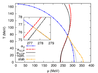
Figure 1: Phase diagram for our starting parameter set fitted to vacuum phenomenology. The inset shows a zoomed-in view close to the CP/LP. The solid grey line denotes the first-order phase boundary for homogeneous matter, the orange dot-dashed line is the boundary of the instability region. The remaining lines denote the position of the roots of the GL coefficients $\alpha_{2}$ (blue dot-dot-dashed), $\alpha_{4,CP}$ (black dotted) and $\alpha_{4,LP}$ (red dashed). Above the LP the $\alpha_{2}$ line corresponds to the second-order boundary between the homogeneous broken and two-flavor restored phase.

In order to get further insight into the nature of the splitting between the CP and the LP, we now investigate the effect of varying the model parameters associated with the third flavor, namely the KMT coupling $K$ and the strange current mass $m_{s}$ on the location of the two points. A first useful observation is that the equation $\alpha_{4,b}=0$ (see Eq. (30)) does not depend on any of these two, and therefore the location of the LP will only be affected by changes in the $\alpha_{2}=0$ line.

We start by showing in Fig. 2 the influence of the strange current mass on the location of the CP and the LP, varying $m_{s}$ from 300 MeV toward zero. As can be seen from the figure, the points move rather slowly for large and moderate values of $m_{s}$ but speed up when the current mass gets smaller. As expected, with decreasing $m_{s}$ the location of the CP moves to lower chemical potentials, until eventually it hits the temperature axis and the phase transition between the homogeneous phases becomes first order at all chemical potentials. With our parameter set, this occurs for a strange current mass of around 10 MeV. This agrees well with the corresponding value of $m_{s}$ found in Ref. Fukushima (2008) within a three-flavor PNJL model with three-momentum cutoff, giving additional support to our parameter choice.

The LP on the other hand follows a different trajectory, significantly splitting from the CP and moving toward lower temperatures as the current strange mass decreases. In order to better understand this behavior, we show in Fig. 3 for two different values of $m_{s}$ the curves where the relevant GL coefficients vanish. We see that for lower $m_{s}$ the $\alpha_{4,CP}$ line moves toward the temperature axis (in particular around the $\alpha_{2}$ line), thus explaining the corresponding movement of the CP. On the other hand, recalling that $\alpha_{4,LP}$ does not change at all, the relatively mild change of $\alpha_{2}$ suggests that the LP moves only little. Nevertheless, together with the shape of the $\alpha_{4,LP}=0$ line, it explains why the LP goes down in temperature when $m_{s}$ is reduced.

Again we should however pay attention to the ordering of the phase transitions. Unlike for the realistic mass case in Fig. 1, we find that for small values of $m_{s}$ the homogeneous first-order phase boundary is to the “right” of the inhomogeneous instability line. In this case, coming from the two-flavor chirally restored phase and reducing the chemical potential, the homogeneous first-order transition takes place first and invalidates our analysis for the LP and the second-order phase transition to the inhomogeneous phase. More precisely, we find that the LPs indicated in Fig. 2 should not be trusted for $m_{s}\leq 50$ MeV, while at least part of the instability line still lies to the right of the homogeneous first-order line until $m_{s}\simeq 40$ MeV. Below this value it moves completely behind it and it is then likely that the inhomogeneous phase disappears from the phase diagram.

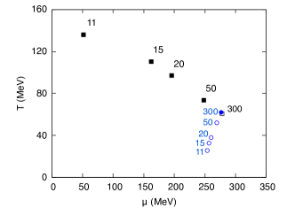
Figure 2: Locations of the CP(black squares) and LP(blue dots) for different values of $m_{s}$ (as indicated, in MeV). Filled (open) symbols denote the cases in which the GL analysis used to determine them is reliable (not reliable).

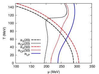
Figure 3: Roots of GL coefficients for $m_{s}=20$ MeV (black) and $m_{s}=50$ MeV (red). The dashed lines correspond to $\alpha_{2}$, the dotted ones to $\alpha_{4,CP}$. The solid blue line indicates the root of $\alpha_{4,LP}$, which is independent of $m_{s}$.

In the above analysis, in order to single out the effects of varying a single parameter on the phase structure of the model, we decided not to refit completely all the vacuum observables but simply varied $m_{s}$ while keeping all the other parameters fixed. Changing the current strange quark mass turns out to have a very small effect on the value of the vacuum constituent quark mass for light quarks, whose value is known to strongly affect the phase transition in the light sector. This was however not the case for the six-quark coupling $K$, as simply decreasing it while keeping all the other parameters fixed quickly leads to unreasonably small $M_{\ell}^{(vac)}$ and consequently to the disappearance of both CP and LP from the phase diagram. In order to work around this limitation, we decided to refit the four-fermion coupling $G$ together with $K$ in order to give the same $M_{\ell}^{(vac)}$ as in our starting parameter set. The resulting locations of the CP and the LP for different values of $K$ (and refitted $G$) are shown in Fig. 4. There we can see that, after performing the refit, the locations of both points depend only very little on $K$ (note the scale!). Within this scale, they follow again different trajectories. As expected, the two points agree for $K=0$, reproducing the known two-flavor limit as the third flavor in this case decouples completely. As $K$ increases, the two split and the LP moves above the CP. Up to $K\Lambda^{5}=160$ the situation is qualitatively similar to the one discussed in Fig. 1, i.e., the inhomogeneous phase completely covers the first-order phase boundary, invalidating the GL results for the CP. The trend reverses if we consider extremely high values of the six-quark coupling: For $K\Lambda^{5}\gtrsim 170$ the CP reappears in the phase diagram, while the GL result for the LP can no longer be trusted. We stress again that all these variations occur in a very limited range of temperatures and chemical potentials, as can be seen by the scale in the figure.

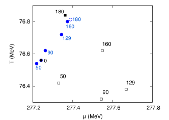
Figure 4: Locations of the CP(black squares) and LP(blue dots) for different values of $K\Lambda^{5}$. For $K=0$ the two points coincide. Filled (open) symbols denote the cases in which the GL analysis used to determine them is reliable (not reliable).

Finally, we would like to comment on the situation at higher densities. From the two-flavor NJL model it is known that at higher chemical potentials a second inhomogeneous phase appears whose physical nature is unclear and which we termed “inhomogeneous continent” Carignano and Buballa (2012a). The corresponding phase boundary can also be determined by the stability analysis, and we find that for the three-flavor model the inhomogeneous continent exists as well. In fact, the existence of this phase was already reported in Ref. Moreira et al. (2014) for $T=0$. Moreover, these authors found that, as a consequence of the KMT interaction a third inhomogeneous phase appears between the usual inhomogeneous “island” and the continent. At the lower-$\mu$ end this new phase is reached from the two-flavor restored phase via a second-order phase transition whereas at the upper end there is a first-order transition back to the restored phase.

In our calculations, i.e., with our regularization and parametrization, we do not see this intermediate inhomogeneous phase, but we find a behavior which could be seen as precursor of this phase and might allow us to shed some light on its nature: Within our starting parameter set, we find that, as we increase the chemical potential beyond the second-order transition from the inhomogeneous island to the restored phase, the function $\Gamma^{-1}_{\ell}$ starts developing a new minimum for large values of $\bf{q}^{2}$, which gradually approaches zero. However, before the instability is reached, the partial chiral-symmetry restoration in the strange sector takes place, leading to a steep decrease of the dynamical strange quark mass and pushing the minimum up away from zero. The minimum then decreases again and eventually reaches zero at the onset of the inhomogeneous continent.

At least qualitatively, this behavior and that observed in Ref. Moreira et al. (2014) can be understood from Eq. (42). Consider a point on the second-order phase boundary between inhomogeneous and two-flavor restored phase. On this point we have $\Gamma_{\ell}^{-1}=0$, i.e., the expression in square brackets in Eq. (42) vanishes. From this we can see that if we now increase the value of $\delta$, $\Gamma_{\ell}^{-1}$ becomes negative, i.e., the point moves inside the inhomogeneous phase. Hence, increasing $\delta$ increases the size of the inhomogeneous regime, moving the upper phase boundary of the inhomogeneous island upwards and the lower boundary of the continent downwards in $\mu$. The situation is complicated however by the fact that $\delta$ depends on $M_{s,0}$ and thus indirectly on $T$ and $\mu$. As long as $M_{s,0}$ is roughly constant, we have $\delta\propto K/G^{2}$, i.e., increasing $K$ (and simultaneously decreasing $G$ by the parameter refit) enhances the value of $\delta$ and thus of the inhomogeneous region. In contrast, if we keep $K$ fixed but increase the value of $\mu$, the strong decrease of $M_{s,0}$ related to the partial chiral-symmetry restoration in the strange sector lowers $\delta$ considerably, in our case preventing an early onset of the continent. If on the other hand the decrease of $M_{s,0}$ occurs after the second inhomogeneous phase has already started, the related decrease of $\delta$ can shut this phase off again, and the continent reappears only at even higher values of $\mu$. It is possible that this is what happened in Ref. Moreira et al. (2014), and it would be interesting to check whether this scenario is indeed what is occurring within the model regularization and parametrization used in that work.

V Conclusions

In this work we investigated within the NJL model how the formation of inhomogeneous chiral condensates is affected by the inclusion of strange quarks, which are coupled to the light flavors via a KMT determinant interaction, mimicking the effects of the axial anomaly. The use of a Ginzburg-Landau analysis allowed us to infer the location of the critical and the Lifshitz points in a general way without having to specify a shape for the spatial dependence of the chiral condensate. Furthermore, using a complementary stability analysis, we were able to determine the location of the second-order phase transition where inhomogeneous condensates become favored over chirally restored matter. The latter also indicates that it is favorable only for the light quark condensates to become inhomogeneous, whereas no instability was found in the strange quark channel. This does not exclude that an inhomogeneous strange quark condensate is induced by the coupling to the light quarks, but this depends on the favored shape of the spatial modulations.

Our first main result is that the axial anomaly leads to a splitting between the CP of the phase transition for homogeneous matter and the LP associated with the inhomogeneous phase. This splitting turns out generally to be very small, with the exception of the limit of very small strange current quark masses, for which the CP moves toward the temperature axis and eventually disappears from the phase diagram, whereas the LP does not follow the same behavior. For a realistic parameter set fitted to vacuum phenomenology, the two points are nevertheless found to almost coincide for a wide range of values of the six-quark coupling $K$. It is important however to stress that the points do not coincide exactly, and for a wide range of parameters explored in this work we find that the first-order chiral phase transition which is typically present when restricting the model analysis to homogeneous matter is completely covered by the inhomogeneous phase.

A closer inspection of the behavior of the GL coefficients allowed us to better understand the behavior of the two points and the magnitude of their splitting, while our complementary stability analysis let us determine in several cases the location of the phase boundary where the inhomogeneous phase terminates. Consistently with the results of Ref. Moreira et al. (2014), we find an enhancement of the inhomogeneous phase due to the coupling with strange quarks, although, as already mentioned, the effect turns out to be quite small, and we did not witness the appearance of any additional inhomogeneous window in the phase diagram compared with the two-flavor case.

We recall that our study relies on the approximation of small amplitudes (and additionally of small gradients for the GL analysis), so it can only provide a reliable result if we are able to expand about a suitable homogeneous solution, which for simplicity we assumed to be the two-flavor restored phase. It would be tedious but straightforward to extend the method to expand about massive homogeneous solutions in the light-quark sector as well, as we have done in Ref. Buballa and Carignano (2019a) for the two-flavor model away from the chiral limit. We note that in this case we could even study the stability of the homogeneous chirally broken phase against inhomogeneities, while this region was not accessible to our present analysis. But even then we stay restricted to second-order phase transitions. It would therefore be desirable to perform a full numerical evaluation of the model thermodynamic potential in order to obtain the complete phase structure of the model. This would require the introduction of specific Ansätze on the spatial dependence of the chiral condensate and a full numerical diagonalization of the quark Hamiltonian, as done, e.g., in Ref. Carignano and Buballa (2012b). In principle one could also perform an Ansatz-free minimization of the thermodynamic potential within lattice field theory, which has already been applied to analyze inhomogeneous phases in lower-dimensional models Wagner (2007); Heinz et al. (2016); Pannullo et al. (2019); Winstel et al. (2019) but obviously becomes computationally extremely expensive in $3+1$ dimensions. Another way to go beyond the small amplitude constraint would be to perform an extended GL analysis, as done in Carignano et al. (2018b), although the determination of higher order GL coefficients would become significantly more involved due to the additional contributions in the model Lagrangian.

Ultimately we are of course interested in the phase structure of QCD, i.e., one should go beyond effective models and the mean-field approximation. In this context it is interesting to note that in Ref. Fu et al. (2019) hints for an inhomogeneous phase have been found within an FRG study of the QCD phase diagram for $2+1$ flavors. It was found that in a certain regime in the vicinity and above the (homogeneous) chiral phase boundary the mesonic wave-function renormalization constant at vanishing momentum $Z_{\phi}(0)$ becomes negative. As the authors point out, this could indicate an instability toward a spatially modulated regime but the signal is not fully conclusive. In fact, $Z_{\phi}(0)$ basically corresponds to the GL coefficient $\alpha_{4,b}$ in our language, so finding a negative value is a necessary but not a sufficient requirement for an inhomogeneous phase. This becomes clear if we recall that $\alpha_{4,b}$ is proportional to $\frac{d}{d{\bf q}^{2}}\Gamma^{-1}_{\ell}({\bf q}^{2})|_{{\bf q}^{2}=0}$. Hence, a negative value hints at a minimum of $\Gamma^{-1}_{\ell}$ at nonzero ${\bf q}^{2}$ but does not tell whether its value at the minimum is positive or negative. Indeed, in a previous FRG study within the quark-meson model Tripolt et al. (2018) it was found that the static pion two-point function develops a maximum (corresponding to a minimum of $\Gamma^{-1}_{\ell}$) at nonzero ${\bf q}^{2}$ but does not change its sign, so that no instability occurred.

In Ref. Fu et al. (2019) the region with negative $Z_{\phi}(0)$ starts at a chemical potential well below the CP. Hence, if it was indeed related to an instability, it would mean that the CP and most likely the entire first-order phase boundary are covered by an inhomogeneous phase. Unfortunately, a fully conclusive analysis of this issue is extremely involved due to several competing order parameters. In this sense, the analysis performed in our work can act as a guide to give a qualitative picture of the phase structure of dense $2+1$-flavor quark matter as a starting point for these more refined studies to begin with.

Acknowledgments

We thank Dominic Kraatz and Michel Stillger for providing us with their model parameters. We acknowledge support by the Deutsche Forschungsgemeinschaft (DFG, German Research Foundation) through the CRC-TR 211 “Strong-interaction matter under extreme conditions” - project number 315477589 - TRR 211. S.C. has been supported by the projects FPA2016-81114-P and FPA2016-76005-C2-1-P (Spain), and by the project 2017-SGR-929 (Catalonia).

References

- Kumar (2013) L. Kumar, Mod. Phys. Lett. A 28, 1330033 (2013), arXiv:1311.3426 [nucl-ex] .
- (2) B. Friman (ed.) et al., The CBM physics book: Compressed baryonic matter in laboratory experiments, Vol. 814 (2011) pp. 1–980.
- Aoki et al. (2006) Y. Aoki, G. Endrodi, Z. Fodor, S. D. Katz, and K. K. Szabo, Nature 443, 675 (2006), arXiv:hep-lat/0611014 [hep-lat] .
- Fischer (2019) C. S. Fischer, Prog. Part. Nucl. Phys. 105, 1 (2019), arXiv:1810.12938 [hep-ph] .
- Fu et al. (2019) W.-j. Fu, J. M. Pawlowski, and F. Rennecke, (2019), arXiv:1909.02991 [hep-ph] .
- Asakawa and Yazaki (1989) M. Asakawa and K. Yazaki, Nucl. Phys. A 504, 668 (1989).
- Scavenius et al. (2001) O. Scavenius, A. Mocsy, I. N. Mishustin, and D. H. Rischke, Phys. Rev. C 64, 045202 (2001), arXiv:nucl-th/0007030 [nucl-th] .
- Kutschera et al. (1990) M. Kutschera, W. Broniowski, and A. Kotlorz, Phys.Lett. B237, 159 (1990).
- Nakano and Tatsumi (2005) E. Nakano and T. Tatsumi, Phys. Rev. D 71, 114006 (2005).
- Nickel (2009a) D. Nickel, Phys. Rev. Lett. 103, 072301 (2009a), arXiv:0902.1778 [hep-ph] .
- Nickel (2009b) D. Nickel, Phys.Rev. D80, 074025 (2009b), arXiv:0906.5295 [hep-ph] .
- Buballa and Carignano (2015) M. Buballa and S. Carignano, Prog. Part. Nucl. Phys. 81, 39 (2015), arXiv:1406.1367 [hep-ph] .
- Carignano et al. (2010) S. Carignano, D. Nickel, and M. Buballa, Phys. Rev. D82, 054009 (2010), arXiv:1007.1397 [hep-ph] .
- Buballa and Carignano (2019a) M. Buballa and S. Carignano, Phys. Lett. B791, 361 (2019a), arXiv:1809.10066 [hep-ph] .
- Müller et al. (2013) D. Müller, M. Buballa, and J. Wambach, Phys. Lett. B 727, 240 (2013), arXiv:1308.4303 [hep-ph] .
- Moreira et al. (2014) J. Moreira, B. Hiller, W. Broniowski, A. Osipov, and A. Blin, Phys. Rev. D 89, 036009 (2014), arXiv:1312.4942 [hep-ph] .
- Pisarski and Wilczek (1984) R. D. Pisarski and F. Wilczek, Phys. Rev. D29, 338 (1984).
- Fukushima (2008) K. Fukushima, Phys. Rev. D 77, 114028 (2008), erratum-ibid. D 78, 039902, arXiv:0803.3318 [hep-ph] .
- Buballa and Carignano (2019b) M. Buballa and S. Carignano, in PoS(Confinement2018), 202, (2019) arXiv:1906.03241 [hep-ph] .
- Buballa (2005) M. Buballa, Phys. Rept. 407, 205 (2005), arXiv:hep-ph/0402234 .
- Dautry and Nyman (1979) F. Dautry and E. Nyman, Nucl. Phys. A 319, 323 (1979).
- Carignano et al. (2018a) S. Carignano, M. Schramm, and M. Buballa, Phys. Rev. D98, 014033 (2018a), arXiv:1805.06203 [hep-ph] .
- (23) D. Kraatz and M. Stillger, private communication; in preparation .
- Rehberg et al. (1996) P. Rehberg, S. P. Klevansky, and J. Hufner, Phys. Rev. C53, 410 (1996), arXiv:hep-ph/9506436 [hep-ph] .
- Hatsuda and Kunihiro (1994) T. Hatsuda and T. Kunihiro, Phys. Rept. 247, 221 (1994).
- Lutz et al. (1992) M. F. M. Lutz, S. Klimt, and W. Weise, Nucl. Phys. A542, 521 (1992).
- Kohyama et al. (2016) H. Kohyama, D. Kimura, and T. Inagaki, Nucl. Phys. B906, 524 (2016), arXiv:1601.02411 [hep-ph] .
- Carignano et al. (2018b) S. Carignano, M. Mannarelli, F. Anzuini, and O. Benhar, Phys. Rev. D97, 036009 (2018b), arXiv:1711.08607 [hep-ph] .
- Carignano and Buballa (2012a) S. Carignano and M. Buballa, Acta Phys. Polon. Supp. 5, 641 (2012a), arXiv:1111.4400 [hep-ph] .
- Carignano and Buballa (2012b) S. Carignano and M. Buballa, Phys. Rev. D86, 074018 (2012b), arXiv:1203.5343 [hep-ph] .
- Wagner (2007) M. Wagner, Phys. Rev. D76, 076002 (2007), arXiv:0704.3023 [hep-lat] .
- Heinz et al. (2016) A. Heinz, F. Giacosa, M. Wagner, and D. H. Rischke, Phys. Rev. D93, 014007 (2016), arXiv:1508.06057 [hep-ph] .
- Pannullo et al. (2019) L. Pannullo, J. Lenz, M. Wagner, B. Wellegehausen, and A. Wipf, in Lattice 2019, Wuhan, Hubei, China, June 16-22, 2019 (2019) arXiv:1909.11513 [hep-lat] .
- Winstel et al. (2019) M. Winstel, J. Stoll, and M. Wagner, (2019), arXiv:1909.00064 [hep-lat] .
- Tripolt et al. (2018) R.-A. Tripolt, B.-J. Schaefer, L. von Smekal, and J. Wambach, Phys. Rev. D97, 034022 (2018), arXiv:1709.05991 [hep-ph] .