The Two LIGO/Virgo Binary Black Hole Mergers on 2019 August 28 Were Not Strongly Lensed

Abstract

The LIGO/Virgo gravitational wave events S190828j and S190828l were detected only 21 minutes apart, from nearby regions of sky, and with the same source classifications (binary black hole mergers). It is therefore natural to speculate that the two signals are actually strongly lensed images of the same merger. However, an estimate of the separation of the (unknown) positions of the two events requires them to be $>10\arcdeg$ apart, much wider than the arcsecond-scale separations that usually arise in extragalactic lensing. The large separation is much more consistent with two independent, unrelated events that occurred close in time by chance. We quantify the overlap between simulated pairs of lensed events, and use frequentist hypothesis testing to reject S190828j/l as a lensed pair at 99.8% confidence.

1 Introduction

On 2019 August 28 UT, the Advanced Laser Interferometer Observatory (LIGO; LIGO Scientific Collaboration et al. 2015) and the Virgo Gravitational-Wave Observatory (Virgo; Acernese et al. 2015) detected two gravitational wave (GW) signals, S190828j and S190828l, that were separated in time by roughly 21 minutes (LIGO Scientific Collaboration and Virgo Collaboration, 2019a, b). Both signals were consistent with coming from binary black hole (BBH) mergers, and were both highly significant detections with false alarm rates of 1 per $3.7\times 10^{13}$ years and 1 per $6.8\times 10^{2}$ years, respectively. Rapid localization using BAYESTAR (Singer & Price, 2016) revealed that the events had similarly-shaped localization probability contours, and that they appeared to originate from nearby regions of sky. Together, these observations are suggestive of a possible strong lensing origin.

Recent articles have proposed that detections of strongly lensed GWs should be relatively common (Broadhurst et al., 2018, 2019), while others have predicted that they should be relatively rare (Dai et al., 2017; Ng et al., 2018; Oguri, 2018; Smith et al., 2018). Definitively establishing a strong-lensing origin for S190828j/l would be an important advance toward the resolution of this question. By simulating BAYESTAR sky maps of lensed pairs of BBH mergers and comparing them to the contents of the publicly available LIGO/Virgo alerts and localizations of S190828j/l, we show in this Letter that the two events are not the result of strong lensing, but rather are unrelated BBH mergers that occurred close in time and relatively close in space.

2 Strong Lensing

In the strong-lensing interpretation of S190828j/l, the two events correspond to two lensed images of the same BBH merger. The images form due to the curvature of space-time by an unknown intervening mass along the line of sight. The deflector may be a galaxy (e.g., Bolton et al., 2006), a galaxy cluster (e.g., Broadhurst et al., 2005), a dwarf galaxy (e.g., Quimby et al., 2014), an extragalactic star (Chang & Refsdal, 1979), an extragalactic field of stars (Schneider & Weiss, 1987), or even a cosmic string (Hogan & Narayan, 1984). The image multiplicity is set by the mass distribution of the lens and its orientation with respect to the GW source, and in principle can be much larger than two. “Double” or “quad” images are the most common products of galaxy-scale lensing (Treu, 2010), while rich clusters routinely produce more than four images of background sources (e.g., Umetsu et al., 2016). In the strong-lensing scenario, remaining images of S190828j/l, if they exist, were either too faint to trigger alerts, arrived when the interferometers were not in observing mode, or may still be yet to arrive.

In the strong-lensing scenario, the lensed images S190828j and S190828l travel along different geometric paths and through geometric potentials to reach us, explaining their 21 minute difference in arrival times. This time-delay effect is a key feature of strong lensing (Refsdal, 1964). Observed time delays in strong lensing systems have ranged from minutes to hours at the low end (e.g., SN iPTF16geu; Goobar et al., 2017; More et al., 2017; Mörtsell et al., 2019), to decades at the high end (e.g., SN Refsdal; Kelly et al., 2015). A strong-lensing hypothesis thus seems, at broad brush, to offer a convenient explanation for the spatial and temporal proximity of S190828j and S190828l. However, as we will show in this Letter, the spatial separation between S190828j and S190828l ($>$10${}^{\circ})$ turns out to be too large and the time delay (21 minutes) too small for lensing to work.

2.1 Effect of Lensing on LIGO Observables

Before presenting our analysis of the LIGO data, we first review the effects of gravitational lensing on GW strain signals and present some useful scaling relations. In an expanding universe, the leading-order post-Newtonian approximation to the GW strain from a compact binary merger is (cf. Schutz 1986; Holz & Hughes 2005; Nissanke et al. 2010)

$$h(f)=\Theta\frac{(1+z)\mathcal{M}}{D_{\mathrm{L}}}(\pi(1+z)\mathcal{M}f)^{2/3}e^{-i\Psi(f)}.$$ (1)

Here, the factor $\Theta$ encapsulates all of the dependence on the orientation and sky position of the binary, $z$ is the redshift of the binary, $f$ is the GW frequency, $D_{\mathrm{L}}$ is the luminosity distance, $\Psi(f)$ is the leading-order phase as a function of frequency, and $\mathcal{M}$ is the chirp mass defined in terms of the component masses as $\mathcal{M}=(m_{1}m_{2})^{3/5}(m_{1}+m_{2})^{-1/5}$.

One can recast this in terms of the redshifted chirp mass $\mathcal{M}_{z}=(1+z)\mathcal{M}$ (and similarly the redshifted component masses $m_{1,z}=(1+z)m_{1}$ and $m_{2,z}=(1+z)m_{2}$) as

$$h(f)=\Theta\frac{\mathcal{M}_{z}}{D_{\mathrm{L}}}(\pi\mathcal{M}_{z}f)^{2/3}e^{-i\Psi(f)}.$$ (2)

The redshifted masses are also referred to as the observer frame masses, in contrast to the physical source frame masses. Strong lensing does not alter the redshifted, observer-frame masses. The apparent luminosity distance, however, is modified by the lensing magnification $\mu$ according to

$$D_{L}^{\prime}=\frac{D_{L}}{\sqrt{|\mu|}}.$$ (3)

2.2 Angular and Temporal Scales for Lensing

The angular scale of separation between a pair of lensed images is given by the Einstein angle $\theta_{\mathrm{E}}$, which in the case of a point lens takes the form

$$\theta_{\mathrm{E}}=\left(\frac{4GM}{c^{2}}\frac{D_{ls}}{D_{l}D_{s}}\right)^{1/2},$$ (4)

where $M$ is the mass of the lens, $D_{l}$ is the angular diameter distance to the lens, $D_{s}$ is the angular diameter distance to the source, and $D_{ls}$ is the angular diameter distance between the lens and the source (Schneider et al., 1992). In addition to bound structures, cosmic strings, hypothesized one-dimensional topological defects in spacetime, may also produce lensing, but the image separation has a different dependence on distance than in Equation 4 (Pogosian et al., 2003; Morganson et al., 2010). The Einstein angle $\theta_{E}$ of a cosmic string is given by

$$\theta_{\mathrm{E}}=\frac{8\pi G\mu}{c^{2}}\sin i\frac{D_{ls}}{D_{s}},$$ (5)

where $\mu$ is the string “tension” and $i$ is the angle that the cosmic string forms with the line of sight. There are observational limits on cosmic string tension $G\mu/c^{2}$ from optical surveys (Morganson et al., 2010), the cosmic microwave background (Planck Collaboration et al., 2014), and even GWs (Abbott et al., 2018).

Dimensionally, Equation 4 can be expressed as

$$\theta_{\mathrm{E}}=\left(\frac{M}{10^{11.09}M_{\odot}}\right)^{1/2}\left(\frac{D_{l}D_{s}/D_{ls}}{\mathrm{Gpc}}\right)^{-1/2}\,\mathrm{arcsec}.$$ (6)

Similarly, setting $\sin i=1$ in Equation 5 for the greatest possible magnification, we obtain

$$\theta_{\mathrm{E}}=5.2\left(\frac{G\mu/c^{2}}{10^{-6}}\right)\left(\frac{D_{ls}}{D_{s}}\right)\,\mathrm{arcsec}.$$ (7)

Plugging numbers into Equations 6 and 7 gives the spatial scale for lensing in various mass and distance regimes, which we have plotted in Figure 1, assuming a Planck Collaboration et al. (2016) cosmology. By comparing the angular separation S190828j/l sky maps to the scales for lensing in Figure 1 across 15 decades in mass, we will show in the next section that the lensing separations associated with even the most massive bound structures in the universe are many orders of magnitude smaller than those required to explain S190828j/l.

Finally, in most plausible astrophysical lensing scenarios, such as galaxy-galaxy lensing, galaxy-cluster lensing, and extragalactic stellar microlensing, time delays increase as image separations increase. This can be understood as a consequence of geometry: for fixed source and lens positions, larger image separations (due e.g., to increasing the lens mass) lead to larger differences in path length, which in turn lead to larger time delays. For a given lens, the magnitude of the time delay between two lensed images depends sensitively on the location of the unlensed source relative to the lens. For microlensing by stars, typical time delays are a few microseconds (Moore & Hewitt, 1996); for galaxy-galaxy lensing, time delays typically range from a few hours to a few months (Oguri & Marshall, 2010; Goldstein & Nugent, 2017); and for cluster lensing, time delays can be as high as several decades (e.g., Kelly et al., 2015). As Figure 1 shows, the $\gtrsim 10^{\circ}$ separation of S190828j/l requires a lens with a mass roughly $10^{6}$ times that of the largest known bound structures in the Universe. As larger image separations in general correlate with larger time delays, achieving a 21 minute time delay with such a large lens would require exceptional source-lens alignment, assuming a spherically symmetric mass distribution. The short time delay and large separation of S190828j/l futher strain the lensing interpretation.

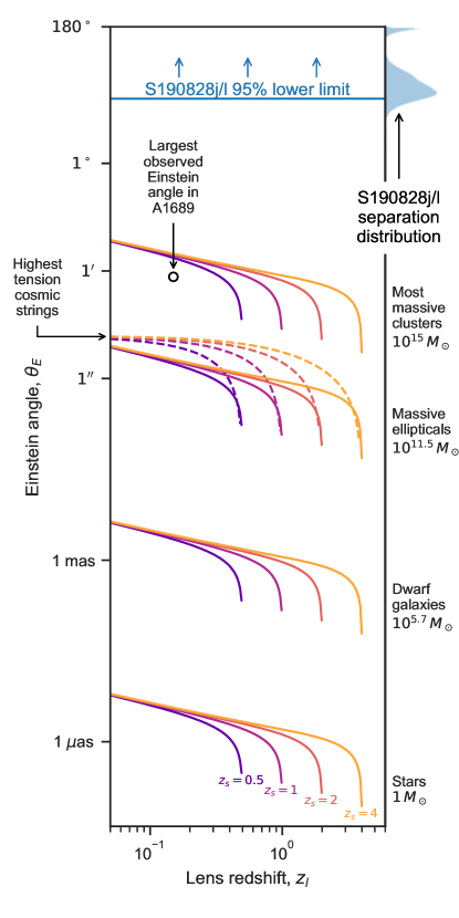
Figure 1: Einstein angle $\theta_{\mathrm{E}}$ as a function of lens redshift $z_{l}$ of a variety of strong lensing systems: extragalactic stars or star fields (“Stars”), dwarf galaxies, elliptical galaxies, and superclusters, the most massive bound structures in the universe. The posterior probability distribution of the separation of S190828j and S190828l is shown on the right (also in the top panel of Figure 3), and the 95% lower limit on the separation is shown as the horizontal blue line near the top.

3 Analysis of the public LIGO/Virgo data

To test the strong lensing hypothesis described in the previous section, we downloaded the initial BAYESTAR localizations (Singer & Price, 2016; LIGO Scientific Collaboration and Virgo Collaboration, 2019a, b) of S190828j and S190828l and plotted them in Figure 2. We also inspected the refined LALInference localizations (Veitch et al., 2015; LIGO Scientific Collaboration and Virgo Collaboration, 2019c, d).

Each of the localizations is bimodal, consisting essentially of an annulus determined by the time delay on arrival at Hanford and Livingston, carved into two opposing segments by the sensitivity nulls in the Hanford and Livingston antenna patterns. The 90%-credible regions of the two localizations do not overlap.

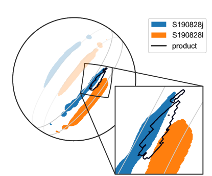
Figure 2: The BAYESTAR 90% credible localization regions of the two mergers and their joint product. The two parallel gray lines are lines of constant time delay between Hanford and Livingston and are separated by 13$\arcdeg$. The 90% credible areas of S190828j and S190828l are 587 and 948 deg² respectively, and the 90% credible region of their joint product is 94 deg². For LALInference, the events’ 90% credible areas are 228 and 359 deg² respectively, with a joint 90% credible area of 11 deg².

Nonetheless, if we assume that they are lensed images with negligible separation compared to the LIGO/Virgo localization uncertainty, then we can form a joint localization region by multiplying and then normalizing the two sky maps. Denoting the two localizations as $p(\hat{\mathbf{n}})$ and $q(\hat{\mathbf{n}})$, the joint localization is

$$r(\hat{\mathbf{n}})=\frac{p(\hat{\mathbf{n}})q(\hat{\mathbf{n}})}{\int p(\hat{\mathbf{n}}^{\prime})q(\hat{\mathbf{n}}^{\prime})\,d\Omega^{\prime}}.$$ (8)

Operationally, since the sky maps are stored discretely as normalized arrays of equal-area HEALPix pixels, this is evaluated as

$$r_{i}=\frac{p_{i}q_{i}}{\sum_{j}p_{j}q_{j}},$$ (9)

where the sum is over pixels. This joint localization is shown as the black contour in Figure 2. The denominator of this expression can be interpreted as a Bayes factor comparing the lensed and unlensed hypotheses (Haris et al., 2018; Hannuksela et al., 2019), and is equal to

$$\mathcal{B}^{L}_{U}=\int p(\hat{\mathbf{n}}^{\prime})q(\hat{\mathbf{n}}^{\prime})\,d\Omega^{\prime}={\sum_{i}p_{i}q_{i}}=3.9\times 10^{-9},$$ (10)

disfavoring lensing at about the $6$-$\sigma$ level. For LALInference, the Bayes factor of $\mathcal{B}^{L}_{U}=5.7\times 10^{-10}$ rejects lensing even more strongly.

Alternatively, we can assume that the events are lensed images but with no prior assumption about the separation. We can then calculate the joint probability distribution of the image separation $\theta$ and relative magnification $\left|\mu_{1}/\mu_{2}\right|$. In the geometric optics limit that produces multiple distinct images, lensing is achromatic and therefore it does not alter the apparent detector-frame masses. Its only impacts are to alter the arrival time, sky location, and apparent luminosity distance of the signal. Therefore $\left|\mu_{1}/\mu_{2}\right|=(D_{\mathrm{L},2}/D_{\mathrm{L},1})^{2}$. Assuming a uniform prior on sky location, the posterior distribution of separation and relative magnification is shown in Figure 3. The relative magnification is consistent with unity; it is roughly log-normally distributed such that $\log_{10}\left|\mu_{1}/\mu_{2}\right|=0.10^{+0.56}_{-0.53}$. For LALInference, the relative magnification is $\log_{10}\left|\mu_{1}/\mu_{2}\right|=0.21_{-0.50}^{+0.54}$.

The separation distribution has two modes containing comparable probability mass, corresponding to the possibilities that the two images are on either adjacent or opposite sections of the triangulation rings. The adjacent mode is favored over the opposite mode by a ratio of $1.2:1$. The first mode is at $\theta=22\arcdeg^{+27\arcdeg}_{-11\arcdeg}$ and the second is at $\theta=161\arcdeg^{+13\arcdeg}_{-31\arcdeg}$. There is only a $\approx 0.01\%$ chance that the separation is smaller than 1$\arcdeg$. For the LALInference localization, the adjacent mode is favored over the opposite mode by a factor of $6.3:1$. The two modes are at $\theta=19\arcdeg_{-10\arcdeg}^{+20\arcdeg}$ and $\theta=160\arcdeg_{-38\arcdeg}^{14\arcdeg}$, respectively, and there is only a $\approx 0.007\%$ chance that the separation is smaller than $1\arcdeg$.

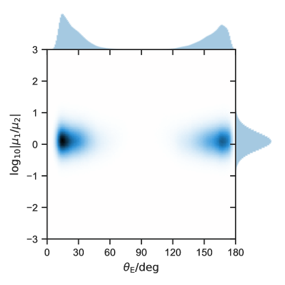
Figure 3: Joint posterior probability distribution of the relative magnification and separation of the images. The separation is constrained to be $>1$ deg at $\approx 99.99\%$ confidence. The relative magnification is consistent with unity, with an uncertainty of about half a decade in either direction.

4 Analysis of Simulated Localizations

To evaluate whether S190828j and S190828l are consistent with a strong lensing origin, we carried out a suite of simulations providing an estimate of the distribution of sky maps that LIGO/Virgo would have observed if:

1. H1, L1, and V1 detected two GW events at the exact times of S190828j and S190828l, corresponding to two lensed images of the same BBH merger.

2. H1, L1, and V1 detected two GW events at the exact times of S190828j and S190828l, corresponding to independent GW signals produced by two unrelated BBH mergers.

The key difference between Cases 1 and 2 is that in Case 1, the true sky locations and the signal-to-noise ratios of the GW signals are tightly correlated due to lensing, whereas in Case 2, they are independent.

4.1 Detector Sensitivity

The sensitivities of the GW detectors in our simulation were matched to the performance of LIGO and Virgo around the time of S190828j/l. LIGO/Virgo do not publish live noise curves. However, the Gravitational Wave Open Science Center’s Gravitational-Wave Observatory Status page for August 28 gave the binary neutron star range between the times of S190828j and S190828l as follows: H1, 113 Mpc; L1, 135 Mpc; V1, 47 Mpc. To approximate the sensitivity of the LIGO and Virgo detectors around the time of the two events, we took the aLIGOMidHighSensitivityP1200087 and AdVMidHighSensitivityP1200087 noise curves from LALSimulation and applied constant scale factors to them in order to match the aforementioned binary neutron star range.

4.2 Source Distribution

We obtained the distribution of source parameters by simulating a uniform-in-comoving-volume population of binary black hole mergers with source frame component masses distributed uniformly in log mass in $[5,50]$ $M_{\odot}$ and aligned component spins uniformly distributed in $[-0.99,0.99]$. This matches the “uniform in log” distribution used to estimate BBH merger rates in Abbott et al. (2019). It does not matter that the source population assumes a particular mass function and no lensing, because it is simply a construct to generate a set of binaries with observer frame masses that are broadly consistent with what LIGO/Virgo has observed. Source locations are isotropic but confined to the intersection of the 99.9999999997% credible regions of S190828j and S190828l (with an area of 6800 deg²) to be broadly consistent with the observed positions of the two events. Signals were injected into Gaussian noise and recovered using matched filtering. Only events that registered an SNR $>4$ in at least 2 detectors and a network SNR $>12$ were kept. For every surviving event, we ran sky localization with BAYESTAR. (We did not run LALInference because it would have been computationally prohibitive.)

4.3 Strongly Lensed Events Simulation

The lensed population is constructed as follows. We draw $10^{5}$ independent samples from the source parameter distribution. Each sample is injected into a stretch of Gaussian noise at a fixed time $t_{0}$. Then the sample is moved to a new random sky location that is drawn uniformly from a cone with a radius of $30\arcsec$ centered on the old sky location, consistent with the largest observed lensing separations from Figure 1. The new apparent luminosity distance is drawn from a log-normal distribution with a width of 0.25 dex centered on the old distance, consistent with the 0.5 dex scatter in relative magnification inferred in Figure 3. It is then injected again into another independent stretch of Gaussian noise at a fixed time $t_{0}+21\,\mathrm{min}$. Pairs of events that pass the detection thresholds at both sidereal times are kept. The lensed population consists of $N_{\mathrm{lensed}}=696$ pairs of events.

4.4 Independent Events Simulation

The independent events population is constructed in a similar manner. We draw $10^{5}$ independent samples form the source parameter distribution and inject them at a time $t_{0}$, and keep the ones that pass the detection thresholds. Then we draw another $10^{5}$ independent samples and inject them at a time $t_{0}+21\,\mathrm{min}$. Events from the first and second group of $10^{5}$ that pass the detection thresholds are matched pairwise. The independent events population consists of $N_{\mathrm{independent}}=989$ pairs of events.

4.5 Frequentist Hypothesis Testing

We employ two closely related test statistics to quantify the overlap between each pair of events. The first is the Bhattacharyya coefficient (Bhattacharyya, 1943), $F(p,q)=\sum_{i}\sqrt{p_{i}q_{i}}$, which in the application to GW localizations has also been referred to as the fidelity (Vitale et al., 2017). The second is the Bayes factor defined in Section 3, defined as $G(p,q)=\sum_{i}p_{i}q_{i}$.

We tabulated both test statistics for each pair of simulated events. Figure 4 shows the empirical distribution function of the test statistics $F(p,q)$ and $G(p,q)$ over the simulated events. The value of the test statistics for the S190828j/l pair is shown as a vertical gray line. The corresponding $P$-values for the lensed and independent events hypotheses are shown as horizontal gray lines.

The $P$-values for both test statistics under the independent events hypothesis happen to be the same to two significant digits, about $P_{\mathrm{independent}}=0.85$, very much consistent with S19082j/l being independent events.

None of our lensed simulations had values of the test statistics that were as extreme as S190828j/l. Therefore we can only provide an upper bound on the P-value for the lensed hypothesis of $P_{\mathrm{lensed}}<1/N_{\mathrm{lensed}}=0.0013$, inconsistent with the lensed hypothesis. Performing a larger number of simulations would only strengthen the rejection of the lensed hypothesis.

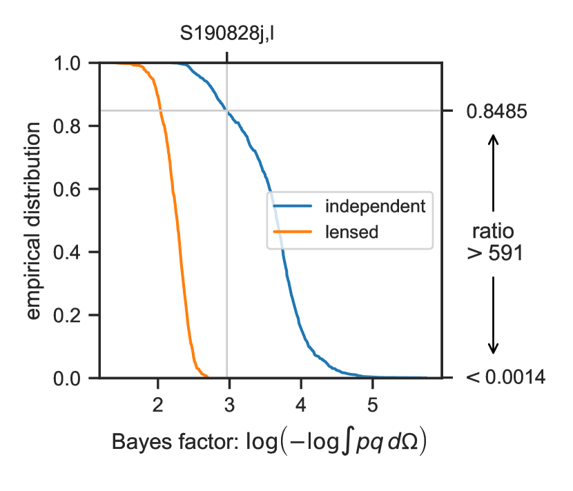
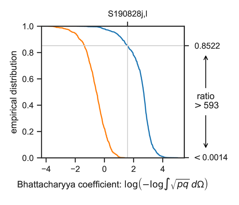
Figure 4: Empirical distribution of the test statistics (left panel: Bayes factor; right panel: Bhattacharyya coefficient) for a population of simulated lensed binary black hole mergers and for a pairs of independent events. The horizontal scale is doubly logarithmic. The values of the test statistics for S190828j/l are shown by the vertical gray lines. $P$-values for S190828j/l under the lensed and independent events hypotheses are shown as horizontal gray lines.

5 Interpretation

It may have been tempting to interpret S190828j and S190828l as strongly lensed images of the same event due to their similar times, similarly shaped localizations, and similar directions on the sky. We offer the following responses to those points.

1. The time coincidence, while striking, is not highly significant by itself.

From April through September, LIGO/Virgo released 21 BBH merger alerts, at an average rate of about $R=0.75$ week^-1. Let us assume that the rate of BBH detections is time-independent. In reality the detection rate does fluctuate with the sensitivity and uptime of the detector network, but accounting for the time variation will not have a significant impact on this line of reasoning. The Poisson probability of $k=2$ or more detections occurring by coincidence during the same period of $T=21$ min is low, $P(k\geq 2)=1-e^{-RT}(1+RT)=1.2\times 10^{-6}$. However, the rate of pairs of events separated by time $T$ is roughly $2P(k\geq 2)/T\approx.061$ year^-1, or one in 16 years. (The rate of double hits was verified by Monte Carlo simulation). After several years of operation, it requires only a little bit of luck for Advanced LIGO/Virgo to observe two events separated by 21 minutes.

2. The localizations look qualitatively similar because the events occurred at similar sidereal times.

The qualitative features of GW localizations are strongly determined by the positions and orientations of the detectors, which rotate with the earth. This is especially true of the present GW detector network, which consists of the two LIGO detectors with nearly aligned antenna patterns, and the much less sensitive Virgo detector. The vast majority of localizations fit the description of a long, thin arc, almost a great circle, arising from the time delay on arrival between Hanford and Livingston, with two polar opposite sections above the antenna pattern maxima favored, and two polar opposite sections that are above the antenna pattern minima strongly disfavored (Singer et al., 2014). One can see this pattern in Advanced LIGO and Virgo’s first and second observing run at a glance in Figure 3 of Abbott et al. (2019) or Figure 8 of Abbott et al. (2019), and even more clearly in Figure 2.5 of Singer (2015) by plotting the localizations of many events in Earth-fixed coordinates. S190828j and S190828l definitely fit the mold. Their localizations look so similar in celestial coordinates because they occurred at similar sidereal times. Their localizations would be likely to look this similar whether or not they were lensed images of the same event.

3. The localizations of the two events rule out astrophysically realistic separations.

Neither localization is very precise, but they are sufficient to constrain the separation of the two unknown sky positions to be $\sim 10\arcdeg$ and rule out sub-arcsecond to sub-arcminute scale separation that would be expected from an astrophysical strong lensing systems. The localizations are entirely inconsistent with each other, and have no significant overlap. In simulations of lensed pairs of events with the same separation in time, we find that there is less than one chance in a thousand of obtaining two localizations that are as inconsistent as S190828j and S190828l, due only to measurement uncertainty. On the other hand, the separation is quite ordinary if we interpret the signals as two unrelated mergers.

6 Conclusion

Neither the intrinsic (mass and spin) parameters of these two events, nor the strain data surrounding them, are publicly available yet. When the waveform parameters or the strain data become available, one can perform additional tests by comparing their waveforms as has been done for previous events by Hannuksela et al. (2019). When the full strain data for all of the present observing run becomes available, one can perform a sub-threshold, mass-constrained search for additional signals with the same waveforms (Li et al., 2019).

It has been argued that a large fraction of LIGO/Virgo BBH signals that have been detected to date may be strongly lensed images of much more distance mergers. Although our results are neutral in that debate, they do show that S190828j and S190828l were probably not lensed images of the same merger.

2D

two–dimensional

2+1D

2+1—dimensional

2MRS

2MASS Redshift Survey

3D

three–dimensional

2MASS

Two Micron All Sky Survey

AdVirgo

Advanced Virgo

AMI

Arcminute Microkelvin Imager

AGN

active galactic nucleus

aLIGO

Advanced LIGO

ASKAP

Australian Square Kilometer Array Pathfinder

ATCA

Australia Telescope Compact Array

ATLAS

Asteroid Terrestrial-impact Last Alert System

GW

gravitational-wave

BAT

Burst Alert Telescope (instrument on Swift)

BATSE

Burst and Transient Source Experiment (instrument on CGRO)

BAYESTAR

BAYESian TriAngulation and Rapid localization

BBH

binary black hole

BHBH

black hole—black hole

BH

black hole

BNS

binary neutron star

CARMA

Combined Array for Research in Millimeter–wave Astronomy

CASA

Common Astronomy Software Applications

CBCG

Compact Binary Coalescence Galaxy

CFH12k

Canada–France–Hawaii $12\,288\times 8\,192$ pixel CCD mosaic (instrument formerly on the Canada–France–Hawaii Telescope, now on the Palomar 48 inch Oschin telescope (P48))

CLU

Census of the Local Universe

CRTS

Catalina Real-time Transient Survey

CTIO

Cerro Tololo Inter-American Observatory

CBC

compact binary coalescence

CCD

charge coupled device

CDF

cumulative distribution function

CGRO

Compton Gamma Ray Observatory

CMB

cosmic microwave background

CRLB

Cramér—Rao lower bound

cWB

Coherent WaveBurst

DASWG

Data Analysis Software Working Group

DBSP

Double Spectrograph (instrument on P200)

DCT

Discovery Channel Telescope

DECam

Dark Energy Camera (instrument on the Blanco 4–m telescope at CTIO)

DES

Dark Energy Survey

DFT

discrete Fourier transform

EM

electromagnetic

ER8

eighth engineering run

FD

frequency domain

FAR

false alarm rate

FFT

fast Fourier transform

FIR

finite impulse response

FITS

Flexible Image Transport System

F2

FLAMINGOS–2

FLOPS

floating point operations per second

FOV

field of view

FTN

Faulkes Telescope North

FWHM

full width at half-maximum

GBM

Gamma-ray Burst Monitor (instrument on Fermi)

GCN

Gamma-ray Coordinates Network

GLADE

Galaxy List for the Advanced Detector Era

GMOS

Gemini Multi-object Spectrograph (instrument on the Gemini telescopes)

GRB

gamma-ray burst

GROWTH

Global Relay of Observatories Watching Transients Happen

GSC

Gas Slit Camera

GSL

GNU Scientific Library

GTC

Gran Telescopio Canarias

GW

gravitational wave

GWGC

Gravitational Wave Galaxy Catalogue

HAWC

High–Altitude Water Čerenkov Gamma–Ray Observatory

HCT

Himalayan Chandra Telescope

HEALPix

Hierarchical Equal Area isoLatitude Pixelization

HEASARC

High Energy Astrophysics Science Archive Research Center

HETE

High Energy Transient Explorer

HFOSC

Himalaya Faint Object Spectrograph and Camera (instrument on HCT)

HMXB

high–mass X–ray binary

HSC

Hyper Suprime–Cam (instrument on the 8.2–m Subaru telescope)

IACT

imaging atmospheric Čerenkov telescope

IIR

infinite impulse response

IMACS

Inamori-Magellan Areal Camera & Spectrograph (instrument on the Magellan Baade telescope)

IMR

inspiral-merger-ringdown

IPAC

Infrared Processing and Analysis Center

IPN

InterPlanetary Network

iPTF

intermediate Palomar Transient Factory

IRAC

Infrared Array Camera

ISM

interstellar medium

ISS

International Space Station

KAGRA

KAmioka GRAvitational–wave observatory

KDE

kernel density estimator

KN

kilonova

LAT

Large Area Telescope

LCOGT

Las Cumbres Observatory Global Telescope

LHO

Laser Interferometer Observatory (LIGO) Hanford Observatory

LIB

LALInference Burst

LIGO

Laser Interferometer GW Observatory

llGRB

low–luminosity gamma-ray burst (GRB)

LLOID

Low Latency Online Inspiral Detection

LLO

LIGO Livingston Observatory

LMI

Large Monolithic Imager (instrument on Discovery Channel Telescope (DCT))

LOFAR

Low Frequency Array

LOS

line of sight

LMC

Large Magellanic Cloud

LSB

long, soft burst

LSC

LIGO Scientific Collaboration

LSO

last stable orbit

LSST

Large Synoptic Survey Telescope

LT

Liverpool Telescope

LTI

linear time invariant

MAP

maximum a posteriori

MBTA

Multi-Band Template Analysis

MCMC

Markov chain Monte Carlo

MLE

maximum likelihood (ML) estimator

ML

maximum likelihood

MOU

memorandum of understanding

MWA

Murchison Widefield Array

NED

NASA/IPAC Extragalactic Database

NIR

near infrared

NSBH

neutron star—black hole

NSBH

neutron star—black hole

NSF

National Science Foundation

NSNS

neutron star—neutron star

NS

neutron star

O1

Advanced ’s first observing run

O2

Advanced ’s second observing run

O3

Advanced ’s and Advanced Virgo third observing run

oLIB

Omicron+LALInference Burst

OT

optical transient

P48

Palomar 48 inch Oschin telescope

P60

robotic Palomar 60 inch telescope

P200

Palomar 200 inch Hale telescope

PC

photon counting

PESSTO

Public ESO Spectroscopic Survey of Transient Objects

PSD

power spectral density

PSF

point-spread function

PS1

Pan–STARRS 1

PTF

Palomar Transient Factory

QUEST

Quasar Equatorial Survey Team

RAPTOR

Rapid Telescopes for Optical Response

REU

Research Experiences for Undergraduates

RMS

root mean square

ROTSE

Robotic Optical Transient Search

S5

LIGO’s fifth science run

S6

LIGO’s sixth science run

SAA

South Atlantic Anomaly

SHB

short, hard burst

SHGRB

short, hard gamma-ray burst

SKA

Square Kilometer Array

SMT

Slewing Mirror Telescope (instrument on UFFO Pathfinder)

S/N

signal–to–noise ratio

SSC

synchrotron self–Compton

SDSS

Sloan Digital Sky Survey

SED

spectral energy distribution

SFR

star formation rate

SGRB

short gamma-ray burst

SN

supernova

SN Ia

Type Ia supernova (SN)

SN Ic–BL

broad–line Type Ic SN

SVD

singular value decomposition

TAROT

Télescopes à Action Rapide pour les Objets Transitoires

TDOA

time delay on arrival

TD

time domain

TOA

time of arrival

TOO

target–of–opportunity

UFFO

Ultra Fast Flash Observatory

UHE

ultra high energy

UVOT

UV/Optical Telescope (instrument on Swift)

VHE

very high energy

VISTA@ESO

Visible and Infrared Survey Telescope

VLA

Karl G. Jansky Very Large Array

VLT

Very Large Telescope

VST@ESO

VLT Survey Telescope

WAM

Wide–band All–sky Monitor (instrument on Suzaku)

WCS

World Coordinate System

w.s.s.

wide–sense stationary

XRF

X–ray flash

XRT

X–ray Telescope (instrument on Swift)

ZTF

Zwicky Transient Facility

References

- Abbott et al. (2018) Abbott, B. P., Abbott, R., Abbott, T. D., et al. 2018, Phys. Rev. D, 97, 102002, doi: 10.1103/PhysRevD.97.102002
- Abbott et al. (2019) Abbott, B. P., Abbott, R., Abbott, T. D., et al. 2019, Phys. Rev. X, 9, 031040, doi: 10.1103/PhysRevX.9.031040
- Abbott et al. (2019) Abbott, B. P., Abbott, R., Abbott, T. D., et al. 2019, ApJ, 875, 161, doi: 10.3847/1538-4357/ab0e8f
- Acernese et al. (2015) Acernese, F., Agathos, M., Agatsuma, K., et al. 2015, Classical and Quantum Gravity, 32, 024001, doi: 10.1088/0264-9381/32/2/024001
- Astropy Collaboration (2013) Astropy Collaboration. 2013, A&A, 558, A33, doi: 10.1051/0004-6361/201322068
- Bhattacharyya (1943) Bhattacharyya, A. 1943, Bull. Calcutta Math. Soc., 35, 99
- Bolton et al. (2006) Bolton, A. S., Burles, S., Koopmans, L. V. E., Treu, T., & Moustakas, L. A. 2006, ApJ, 638, 703, doi: 10.1086/498884
- Broadhurst et al. (2018) Broadhurst, T., Diego, J. M., & Smoot, III, G. 2018, arXiv e-prints. https://arxiv.org/abs/1802.05273
- Broadhurst et al. (2019) Broadhurst, T., Diego, J. M., & Smoot, III, G. F. 2019, arXiv e-prints. https://arxiv.org/abs/1901.03190
- Broadhurst et al. (2005) Broadhurst, T., Benítez, N., Coe, D., et al. 2005, ApJ, 621, 53, doi: 10.1086/426494
- Chang & Refsdal (1979) Chang, K., & Refsdal, S. 1979, Nature, 282, 561, doi: 10.1038/282561a0
- Dai et al. (2017) Dai, L., Venumadhav, T., & Sigurdson, K. 2017, Phys. Rev. D, 95, 044011, doi: 10.1103/PhysRevD.95.044011
- Goldstein & Nugent (2017) Goldstein, D. A., & Nugent, P. E. 2017, ApJ, 834, L5, doi: 10.3847/2041-8213/834/1/L5
- Goobar et al. (2017) Goobar, A., Amanullah, R., Kulkarni, S. R., et al. 2017, Science, 356, 291, doi: 10.1126/science.aal2729
- Górski et al. (2005) Górski, K. M., Hivon, E., Banday, A. J., et al. 2005, ApJ, 622, 759, doi: 10.1086/427976
- Hannuksela et al. (2019) Hannuksela, O. A., Haris, K., Ng, K. K. Y., et al. 2019, ApJ, 874, L2, doi: 10.3847/2041-8213/ab0c0f
- Haris et al. (2018) Haris, K., Mehta, A. K., Kumar, S., Venumadhav, T., & Ajith, P. 2018, arXiv e-prints, arXiv:1807.07062. https://arxiv.org/abs/1807.07062
- Hogan & Narayan (1984) Hogan, C., & Narayan, R. 1984, MNRAS, 211, 575, doi: 10.1093/mnras/211.3.575
- Holz & Hughes (2005) Holz, D. E., & Hughes, S. A. 2005, ApJ, 629, 15, doi: 10.1086/431341
- Kelly et al. (2015) Kelly, P. L., Rodney, S. A., Treu, T., et al. 2015, Science, 347, 1123, doi: 10.1126/science.aaa3350
- Li et al. (2019) Li, A. K. Y., Lo, R. K. L., Sachdev, S., Li, T. G. F., & Weinstein, A. J. 2019, arXiv e-prints, arXiv:1904.06020. https://arxiv.org/abs/1904.06020