A PSF-based Approach to TESS High quality data Of Stellar clusters (PATHOS) - I. Search for exoplanets and variable stars in the field of 47 Tuc.

Abstract

The TESS mission will survey $\sim$85 % of the sky, giving us the opportunity of extracting high-precision light curves of millions of stars, including stellar cluster members. In this work, we present our project “A PSF-based Approach to TESS High quality data Of Stellar clusters” (PATHOS), aimed at searching and characterise candidate exoplanets and variable stars in stellar clusters using our innovative method for the extraction of high-precision light curves of stars located in crowded environments. Our technique of light-curve extraction involves the use of empirical Point Spread Functions (PSFs), an input catalogue and neighbour-subtraction. The PSF-based approach allows us to minimise the dilution effects in crowded environments and to extract high-precision photometry for stars in the faint regime ($G>13$).

For this pilot project, we extracted, corrected, and analysed the light curves of 16641 stars located in a dense region centred on the globular cluster 47 Tuc. We were able to reach the TESS magnitude $T\sim 16.5$ with a photometric precision of $\sim 1\%$ on the 6.5-hour timescale; in the bright regime we were able to detect transits with depth of $\sim$34 parts per million. We searched for variables and candidate transiting exoplanets. Our pipeline detected one planetary candidate orbiting a main sequence star in the Galactic field. We analysed the period-luminosity distribution for red-giant stars of 47 Tuc and the eclipsing binaries in the field. Light curves are uploaded on the Mikulski Archive for Space Telescopes under the project PATHOS.

1 Introduction

In the last two decades, more than 4000 exoplanets have been discovered and confirmed using spectroscopic and photometric studies. More than 75% exoplanets have been found using the transit method; a strong contribution to this research area came from pioneering photometric surveys, carried out both with ground-based (e.g. SuperWASP, Pollacco et al. 2006) and space telescopes (e.g. CoRoT, Baglin et al. 2006). In last years, the Kepler main mission (Borucki et al. 2010) and the reinvented Kepler/K2 mission (Howell et al. 2014), allowed the astronomical community to develop new techniques to extract and analyse high precision light curves of stars in many Galactic fields and to find thousands of new exoplanets and variable stars (see, e.g., Vanderburg & Johnson 2014; Armstrong et al. 2016; Barros et al. 2016; Aigrain et al. 2016; Libralato et al. 2016a).

Figure 1: Field of view covered by CCD 2 of Camera 3 in Sector-1. The figure shows the stacked image obtained by combining 1282 TESS exposures. The green annulus are the inner and outer bounds of the region containing the stars for which we extracted the light curves ($0.075\leq R\leq 1.5$ degree).

Nevertheless, to date only a few confirmed planets have been found to orbit stars in stellar clusters (e.g., Quinn et al. 2012, 2014; Brucalassi et al. 2014, 2017; Malavolta et al. 2016; Mann et al. 2018). Stellar clusters give us an unique opportunity to understand how exoplanets have formed and evolved. Properties of stars in stellar clusters (e.g., mass, radius, age, and chemical composition) can generally be more reliably measured than for many field stars. For this reason, the discovery and characterisation of exoplanets orbiting stars in stellar clusters allow us to correlate planet and hosting star properties. Moreover, because stellar clusters’ ages span over a wide range that goes from few Myrs up to ten Gyrs, the analysis of exoplanets in different stellar clusters allows us to understand how exoplanets have formed and evolved. In addition, the different chemical properties of the stellar clusters give us the opportunity to understand how the environment has affected the exoplanets’ life.

Despite all these advantages, a few exoplanets have been found in stellar clusters because only few clusters have been studied with Kepler and/or spectroscopic surveys; indeed, searches for exoplanets orbiting stellar cluster members have been hampered by observational difficulties because of the crowding. For this reason, appropriate techniques for the extraction of high-precision light curves of stars in dense environments are mandatory. Recently, studies based on the extraction of light curves from Kepler data of open clusters using the Point Spread Function (PSF) approach (Libralato et al. 2016a) or the differential image analysis (Soares-Furtado et al. 2017) have allowed us to obtain high precision photometric time series for very faint stars located in crowded environments.

In the last year, Kepler passed the baton to the Transiting Exoplanet Survey Satellite (TESS, Ricker et al. 2015), a NASA all-sky survey mission aimed at searching exoplanets around bright stars. During its two-year mission, TESS will observe about 85 % of the sky in 27-day sectors, each one covering $24\times 96$ degree² and most of them containing hundreds of stellar clusters. In every sector, about 20 000 stars are observed in short-cadence mode (2-minute). In addition, TESS produces onboard stacked images of the entire field of view, with a cadence of 30-minute (Full-Frame Images, FFIs). The FFIs allow us to extract light curves for all objects with $V\lesssim 17$ that fall within the field of view of each sector, giving us not only the possibility to widen the search of exoplanets to a huge number of stars, but also to produce results in other fields, like asteroseismology, analysis of Solar System objects (Pál et al. 2018), variable stars, supernovae (e.g. Vallely et al. 2019), and other Galactic and extragalactic sources.

Figure 2: Overview of the Gaia DR2 input catalogue used in this work: panel (a) plots the $(\alpha,\delta)$-coordinates of the sources in the catalogue; panel (b) shows the absolute proper motion distribution for all the stars in the catalogue; panel (c) gives the $G$ versus $G_{\rm BP}-G_{\rm RP}$ CMD for the stars in the catalogue; panel (d) shows the $T-G$ versus $G_{\rm BP}-G_{\rm RP}$ distribution for the stars observed by TESS in the first seven sectors. In magenta the relation adopted to transform TESS magnitudes in Gaia magnitudes. Red and green points in panels (a)-(c) are stars with high probability to be 47 Tuc and SMC members, respectively.

In this work we present our project “A PSF-based Approach to TESS High quality data Of Stellar clusters” (PATHOS), aimed at extracting high precision light curves of sources in stellar clusters in order to find candidate exoplanets and variable stars. For this project we apply our expertise on PSF photometry and astrometry on images of crowded fields. In fact, because of the sampling of TESS ($\sim 21$ arcsec/pixel), also sparse stellar clusters appear to be crowded on TESS images. In our previous works (e.g. Nardiello et al. 2015; Libralato et al. 2016a) we demonstrated that by using as input a high-resolution astro-photometric catalogue and empirical PSFs, we are able to measure the flux of each target star in the catalogue with extreme accuracy, after subtracting all its neighbour stars. Using the PSF-based approach we are able to: (1) extract the light curves of stars in crowded regions; (2) minimise the light-contamination effects due to neighbour stars, improving the photometric precision; (3) extract light curves of faint stars, increasing the number of analysable objects.

In the present work we apply for the first time the PSF-based approach to TESS data, in order to extract high-precision light curves of sources in a very crowded field centred on the globular cluster NGC 104 (47 Tuc). In Section 2 we describe our pipeline for the extraction of raw light curves and their correction. The description of the finding, vetting, and modelling of candidate exoplanets is reported in Section 3. Section 4 is a description of the procedure used to find and analyse variable stars. In Section 5 we compare our pipeline with the most advanced, publicly available pipeline for the extraction of light curves from FFIs. The public data release discussion and a summary of the present work are reported in Section 6 and 7, respectively.

Figure 3: Variation of the zero point between TESS calibrated and instrumental magnitude for Sector-1 TESS observations. Red arrows indicate the points that are out of the plot limits.

2 From Full Frame images to light curves

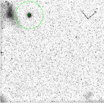
For this pilot work we used FFIs collected in Sector-1. FFIs are obtained on board by co-adding series of 2 s exposures into a 30 minute exposure time image. Observations have been carried out by TESS between 2018 July 25 and 2018 August 22 and cover $\sim 27.83$ days, during which 1282 usable FFIs were generated. The target of this work, 47 Tuc, is located on the CCD 2 of Camera 3. As described in the next Sections, we have extracted the light curves for the stars located in an annulus with $0.075\leq R\leq 1.5$ degree from 47 Tuc centre (as shown in Fig. 1).

2.1 Empirical point spread functions

For our work it is mandatory to compute the best PSF models for each image, both for the extraction of high precision photometry and for the subtraction of the neighbour stars, as explained in Sect. 2.3.

The PSFs of the TESS cameras are highly variable among the large field of view of each CCD (12$\times$12 deg²). To model the PSFs, we used the empirical approach developed by Anderson et al. (2006), adapting the code used for the data collected with the ESO/MPI Wide Field Imager to TESS images. To take into account the spatial variation of the PSF we divided each image in a grid of $9\times 9$ regions. We empirically computed the PSF models independently in each region using bright, not saturated, isolated stars. Each PSF model is defined on a grid of $201\times 201$ points and is super-sampled by a factor 4 with respect to the image pixel.

Adopting this approach, for each position of the CCD we can extract the best, local PSF model by using a bilinear interpolation of the four closest PSFs.

2.2 The input catalogue

For the extraction of the light curves we need an input catalogue that contains the positions and the magnitudes of the stars in the analysed field. We adopted as input catalogue the Gaia DR2 catalogue (Gaia Collaboration et al. 2018). We excluded from the catalogue all the sources with $G>17$ because they are too faint to be measured by TESS (the total flux is $<30$ $e^{-}$/s). For this work, we considered the stars located in a circular region centred in $(\alpha_{0},\delta_{0})=(6.022329,-72.081444)$, i.e. on the centre of 47 Tuc (Goldsbury et al. 2010), and with radius $R=1.5$ degree ($\sim 2\times$ the tidal radius of 47 Tuc). We excluded from the input catalogue all the stars with $R\leq 0.075$ degree because the TESS images are too crowded and saturated within this region. In total, the input catalogue contains 16641 sources.

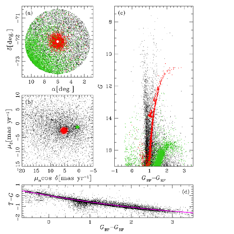
Figure 2 shows an overview of the input catalogue used to extract and analyse the light curves: panels (a), (b), and (c) show the positions, the proper motions and the colour-magnitude diagram (CMD) of the stars analysed in this work. We plotted in red the stars that have high probability to be 47 Tuc members, based on proper motions and parallaxes. We performed the 47 Tuc member selection as follows: first, in the vector point diagram (VPD) of panel (b), we selected by hand the stars that, on the basis of their proper motion, are candidate cluster members. We found the centre of the motion of the cluster by fitting single Gaussians to the $\mu_{\alpha}\cos{\delta}$ and $\mu_{\delta}$ distributions of the selected stars, finding $(\mu_{\alpha}\cos{\delta}_{0},\mu_{\delta})=(5.2,-2.5)$ mas yr^-1. We selected all the stars within $3\sigma$ from the centre of the motion and for these stars we computed the median value of the parallax $\pi=(0.24\pm 0.06)$ mas: we considered candidate cluster members all the stars within $3\sigma_{\pi}$ from the median value of $\pi$. In the same way, we selected Small Magellanic Cloud (SMC) members considering all the stars within $3\sigma$ from the centre of the motion of the SMC ($(\mu_{\alpha}\cos{\delta}_{0},\mu_{\delta})=(0.5,-1.2)$ mas yr^-1) and with parallaxes within $3\sigma$ from the median value $\pi=0.03\pm 0.07$ mas. The SMC high probable members are plotted in green in panels (a), (b), and (c) of Fig. 2.

We transformed the Gaia magnitudes of the stars in the input catalogue into TESS magnitudes using the relation $T-G$ versus $G_{\rm BP}-G_{\rm RP}$ illustrated in panel (d) of Fig. 2. To obtain this relation we cross-matched the TESS target list of the stars observed in the first seven sectors with Gaia DR2 catalogue. We considered all the stars with $G<16$ and $T<16$ and we fitted to the $T-G$ versus $B_{\rm P}-R_{\rm P}$ distribution a 2nd-order polynomial (magenta line in panel (d) of Fig. 2). We found:

$$T=G+a_{0}+a_{1}\times(G_{\rm BP}-G_{\rm RP})+a_{2}\times(G_{\rm BP}-G_{\rm RP})^{2}$$

where $a_{0}=(0.014\pm 0.004)$, $a_{1}=(-0.643\pm 0.007)$, and $a_{2}=(0.055\pm 0.003)$. Transformation from Gaia to TESS magnitudes is significant to minimise systematic residuals, during neighbour subtraction, due to colour terms.

Figure 4: Procedure adopted for the subtraction of the neighbour stars of a target star in the input catalogue. Left-hand panel is one original FFI (tess2018206192942-s0001-3-2-0120-s_ffic.fits): red circle marks the target star (Gaia DR2 4689518492359359488), magenta circles are the neighbour stars in the input catalogue located within 20 pixels (green circle) from the target star. Middle panel is the image of the models of the neighbour stars, that will be subtracted from the original image, to obtain the right-hand panel.

2.3 Light curve extraction

For the extraction of the light curves from TESS images, we used an evolved, improved version of the code img2lc developed by Nardiello et al. (2015, 2016a) for ground-based images and also adopted by Libralato et al. (2016a); Libralato et al. (2016b) and Nardiello et al. (2016b) for the extraction of light curves from Kepler/K2 images of open clusters.

For each FFI, we transformed the $(\alpha,\delta)$-coordinates of the stars in the input catalogue in the image reference system using the WCS keywords and the distortion coefficients in the FITS header of the images. In particular we used the following equation to transform sky coordinates $(\alpha,\delta)$ to geometric distortion corrected pixel coordinates $(U,V)$ (Greisen & Calabretta 2002):

$$\binom{U}{V}={\tt CD}^{-1}\binom{\alpha}{\delta}$$

where CD is the transformation matrix that takes into account the rotation, scaling, and skew of the image. The CD elements are listed in the FITS header. Then, we transformed $(U,V)$ in original pixel coordinates $(x,y)$ using two inversion distortion polynomials, as described by Shupe et al. (2005):

$$x=U+\sum_{p,q}{{\tt AP}{{}_{p}}{{}_{q}}U^{p}V^{q}}\\ y=V+\sum_{p,q}{{\tt BP}{{}_{p}}{{}_{q}}U^{p}V^{q}}$$

where AP and BP are the polynomial coefficients for the terms $U^{p}V^{q}$, and $p+q$ is the order of the polynomial. For all the FFIs analysed in this work $p+q=4$.

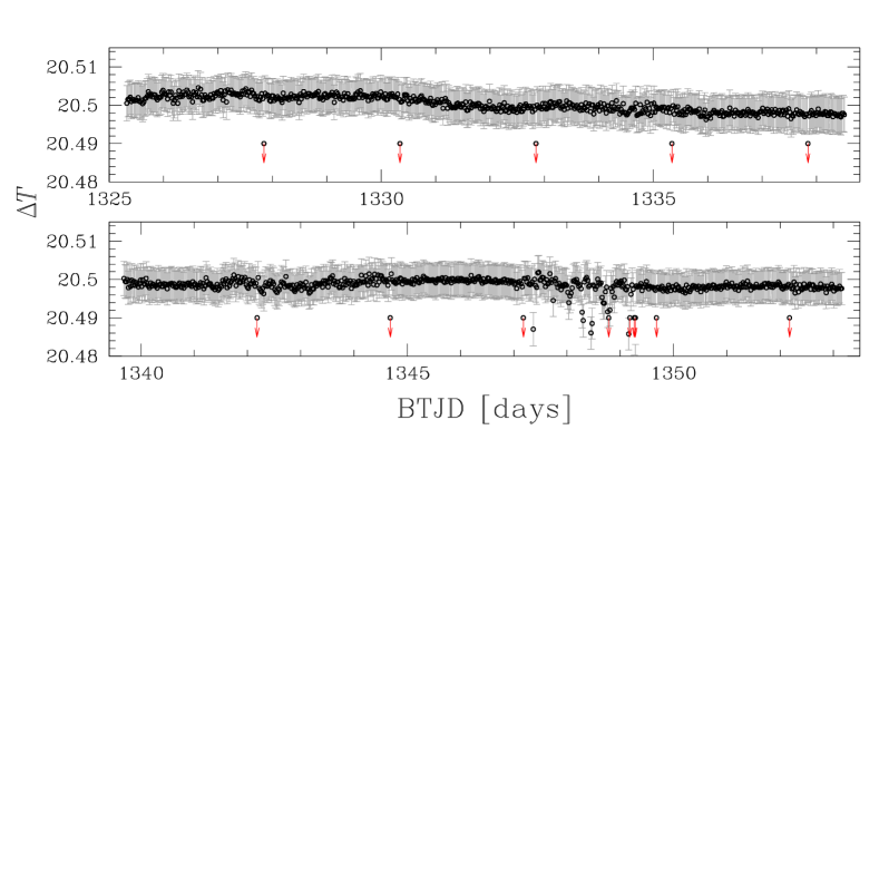
For each image, we used the 200 brightest, un-saturated, and isolated stars in the input catalogue, to derive the photometric zero points between the calibrated TESS magnitude $T_{\rm cal}$ and the instrumental magnitude $T_{\rm inst}$, $\Delta T=T_{\rm cal}-T_{\rm inst}$. In order to compute this quantity, we derived the instrumental magnitude of each star by fitting the local empirical PSF, and then we computed the average value of $T_{\rm cal}-T^{i}_{\rm inst}$, with $i=1,...,200$. Figure 3 shows the variation of $\Delta T$ during the Sector-1.

For each target star in the input list and for each image, the routine considered all the neighbour stars within a radius of 20 pixels and transformed their calibrated magnitudes in instrumental fluxes ($e^{-}/s$) using the previously calculated $\Delta T$. Using the local PSF, the transformed fluxes and the positions, the software made a model of the neighbour stars and then subtracted it from the image. Finally it measured the target flux using both aperture and PSF-fitting photometry on the neighbour-subtracted image. In the case of aperture photometry, we used 4 different aperture sizes: 1, 2, 3, and 4 pixel radius.

Figure 4 shows the procedure for the subtraction of the neighbours from a single image. Left-hand panel shows a $45\times 45$ pixel² subregion of a FFI centred on the target star. Middle panel is the same subregion with the models of the neighbours (located within a radius of 20 pixels from the target star) that are subtracted from the original image. Right-hand panel shows the region after the subtraction of the neighbours.

The fluxes, the epoch of the observations in TESS Barycentric Julian Day (BTJD), the positions on the images and the local sky values were stored in the related light curve file.

Figure 5: Procedure adopted for the correction of the light curve of the star Gaia DR2 4690316359833671040. Panel (a) shows the normalised raw light curve of the star obtained with 3-pixel aperture photometry; panel (b) is the CBV applied to the raw light curve to obtain the corrected light curve shown in panel (c). Red circles are the epochs for which the light curve shows larger systematic effects, due to a pointing problem occurred during the Sector-1.

2.4 Systematic effects correction

The TESS light curves are affected by systematic artifacts, not correlated with the location and the luminosity of the stars on the CCD, but associated with spacecraft, detector and environment. Light curves of stars located on the same detector and observed in the same sector share common systematic trends, allowing us to model them using orthonormal functions, the so-called cotrending basis vectors (CBVs), and correct the systematics that affect the light curves applying to them the CBVs.

To extract the CBVs, we first computed the raw RMS for all the raw light curves and for all the photometric methods. To obtain the raw RMS, we iteratively computed the median value of the light curve and the value $\sigma$, defined as the 68.27th-percentile of the residual from the median, clipping-out at each iteration all the points above and below 3.5$\sigma$ from the median value; after 10 iterations, we defined the RMS as the value of $\sigma$. For a given photometric method, we chose the magnitude interval where the light curves have, on average, lower raw RMS compared to the same light curves obtained with different photometric methods. In this magnitude interval we selected the light curves that showed an ${\tt RMS}<{\tt RMS}_{\rm median}+2\sigma_{\tt RMS}$, where ${\tt RMS}_{\rm median}$ and $\sigma_{\tt RMS}$ are the median of RMS in the considered magnitude interval, and its standard deviation, respectively. Using these stars we extracted the CBVs using a Principal Component Analysis. For each photometric method, we extracted 5 CBVs, that explain 85% of the lightcurves’ variance.

To correct the light curves, we developed a routine that finds the coefficients $A_{i}$ that minimise the expression:

$$F^{j}_{\rm raw}-\sum_{i}{(A_{i}\cdot{\rm CBV_{i}^{j}})}$$ (1)

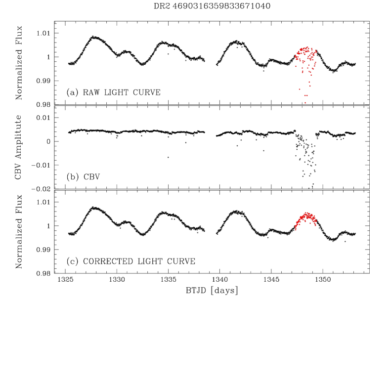
where $F^{j}_{\rm raw}$ is the raw flux of the light curve at the epoch $j=1,...,1282$, and CBV_i is the $i$-th CBV, with $i=1,...,5$. To minimise the expression (1), we used the Levenberg-Marquardt method (Moré et al. 1980). We checked the final results changing the number of CBVs applied to the light curves, and we found that, on average, the application of just the first CBV produced light curves with the lowest RMS. In Fig. 5 we show the procedure adopted for the light curve correction applied to the star Gaia DR2 4690316359833671040 ($T\sim 10$). Panel (a) shows the 3-pixel aperture photometry: in red we highlighted the points of the light curves that show large systematic effects due to pointing problems occurred during the observations of the Sector-1; panel (b) shows the CBV applied to the light curve of panel (a); panel (c) is the cotrended light curve. It is possible to note that the systematic artifacts due to the pointing problems are corrected.

Figure 6: Photometric RMS (panel (a)), P2P RMS (panel (b)), and 6.5-hour RMS (panel (c)) as a function of the TESS magnitude. In panel (a) and (b), the solid lines represent the average trend of the two metrics for the different photometric methods: PSF-fitting (black), 1-pixel aperture (magenta), 2-pixel aperture (blue), 3-pixel aperture (green), and 4-pixel aperture (orange) photometries; light green and grey points are the distributions for the PSF-fitting and 3-pixel aperture photometries. Panel (c) shows the 6.5-hour RMS of the stars for which the best light curve has been chosen: azure line represents the average trend of the distribution; the red dashed line is the theoretical limit of the three RMSs (see text for details).

2.5 Photometric precision

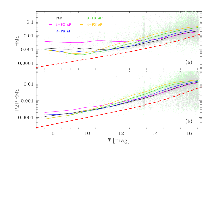
Panel (a) of Fig. 6 shows the RMS as a function of the TESS magnitude for all the stars for which we extracted the light curves. The RMS is computed using the cotrended light curves and adopting the procedure described in Sect. 2.4. For each photometric method, we divided the RMS distribution in bins of 0.75 $T$ magnitude, and, within each bin, we calculated the 3.5$\sigma$-clipped average (with 10 iterations) of the RMS. We interpolated the mean RMS values with a cubic spline. We show in panel (a) of Fig. 6 the interpolated values with black, magenta, blue, green, and orange lines for PSF-fitting, 1-pixel, 2-pixel, 3-pixel, 4-pixel aperture photometries, respectively. The dashed red line is the theoretical RMS limit, obtained considering all the sources of noise (shot noise, sky, Readout Noise, and dark current), and adopting an average Readout Noise of 9 $e^{-}$/pixel, a dark current of 1 $e^{-}$/s/pixel, an average sky value of 100 $e^{-}$ s^-1, and an average aperture of 2 pixels. In the bright regime ($T\lesssim 10.5$) 3-pixel and 4-pixel aperture photometries give the lowest RMS; for stars with $10.5\lesssim T<13.5$ 2-pixel aperture photometry is the best photometry; in the faint regime 1-pixel and PSF-fitting photometry give the best results. For completeness, we plotted in grey and light green the RMS distributions for PSF-fitting and 3-pixel aperture photometries, respectively.

Because the simple RMS parameter is affected by the variability of the stars, we computed the point-to-point RMS (P2P RMS), defined as the 68.27-th percentile of the distribution of the residuals from the median value of $\delta F$, where $\delta F_{j}=F_{j}-F_{j+1}$, and $F_{j}$ and $F_{j+1}$ are the flux values at the epoch $j$ and $j+1$, and $j=1,...,1281$. We derived the mean trends of the P2P RMS distributions for the different photometric methods as done for the RMS. For the following analysis, we used these mean P2P RMS trends to identify, for each star, the best photometry: for each star in the input catalogue with a given $T$ magnitude, we selected the light curve obtained with the photometric method that at the given $T$ returns the lower mean P2P RMS. In this phase we also excluded all the light curves that have $<300$ photometric points and whose mean magnitude differs from that expected from the input catalogue $>2$ magnitudes.

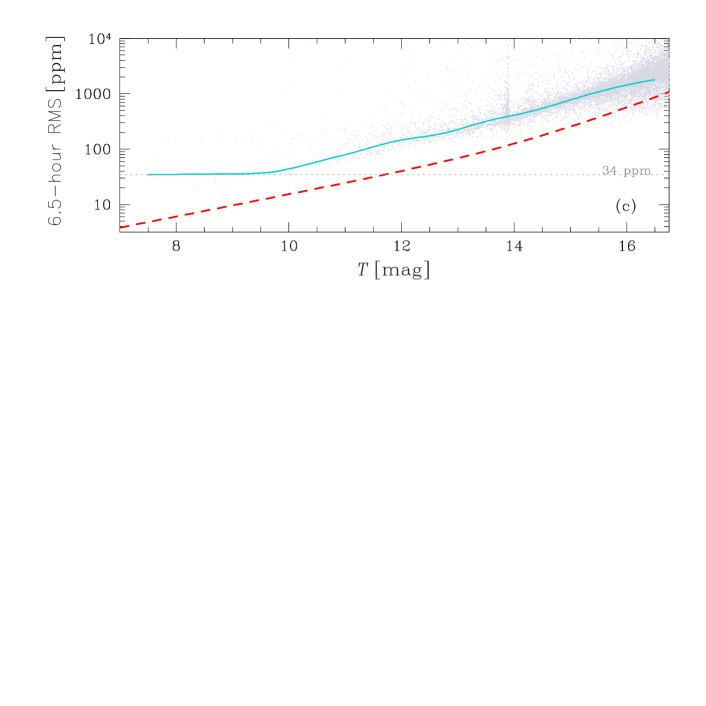
Panel (c) of Fig. 6 shows the 6.5-hour RMS distribution (grey points) for the previously selected light curves. This transit noise 6.5-hour RMS is obtained as described by Gilliland et al. (2011); Gilliland et al. (2015) and Van Cleve et al. (2016): we flattened each light curve interpolating to it a 5th-order spline with 65 break points and removing out the outliers. We computed the standard deviation of a running mean with a window length equal to 6.5-hour (13 points). The azure line in panel (c) is the mean trend of the 6.5-hour RMS distribution, calculated as previously described: the trend reaches a minimum at $\sim 34$ ppm. For $T<10$ the distribution is bi-modal: stars that are not variable or whose period variability is $>6.5$ hours have 6.5-hour RMS$\sim 20$ ppm. The stars with 6.5-hour RMS $\gtrsim$ 30 are highly variable on short timescales and the flattening is not perfect. For stars with $10\lesssim T\lesssim 14$ we are able to detect exoplanets transits with depth $<1$ mmag, while for $T\gtrsim 14$ it is possible to find transits with depth $<0.01$ mag.

3 Candidate exoplanet transit finding

We searched for transiting signals among the light curves selected in the previous section. As described in Sect. 2.5, we flattened all the light curves using 5-th order splines defined on 65 knots. For each light curve, we removed out the outliers and the photometric points with $1347.4<t_{\rm BTJD}<1349.4$, whose photometry is affected by pointing problems and that, despite the cotrending, still have some residual systematic artifacts.

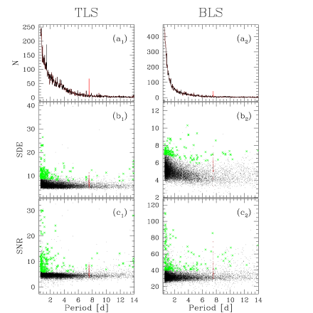
For each light curve we extracted both the Box-fitting Least-Squares (BLS, Kovács et al. 2002) and the Transit-fitting Least Squares (TLS, Hippke & Heller 2019) periodograms. For both techniques we searched for transiting objects having period $0.6\leq P\leq 14$ days, and for each star we extracted the parameters useful to discriminate between light curves with and without candidate transits, such as the Signal Detection Efficiency (SDE), the Signal-to-Noise Ratio (SNR), the depth of the transit. To detect candidate transits we performed two independent analysis on BLS and TLS outputs and at the end we joined the results.

In Fig. 7 we summarise the procedure adopted for the selection of candidate transiting exoplanets both for TLS (left panels) and BLS (right panels) technique. As described in Nardiello et al. (2015), we excluded spurious periods due to systematic errors by constructing the histogram of the period and removing the stars that form the spikes in the histogram: the red spike ($\sim 7.5$ d) in panels (a₁) and (a₂) represents the stars we removed. In a second step, we divided the distributions of SDE (SNR) in period intervals $\delta P=0.5$ d and, within each bin, we calculated the 3$\sigma$-clipped mean value of SDE (SNR), $\overline{{\rm SDE}}$ ($\overline{{\rm SNR}}$), and its standard deviation $\sigma_{\rm SDE}$ ($\sigma_{\rm SNR}$). We interpolated the mean points with a spline and we saved all the stars with ${\rm SDE}>\overline{{\rm SDE}}+3\times\sigma_{\rm SDE}$ and ${\rm SNR}>\overline{{\rm SNR}}+3\times\sigma_{\rm SNR}$. We excluded all the stars having transit depths $>5$%. In panels (b) and (c) the stars that passed the selection criteria are plotted in green: we recovered 186 stars and 145 stars in the case of TLS and BLS, respectively, with 63 stars in common.

Finally we visually inspected the candidate transits that passed the selections to exclude false alarms. We found 7 interesting objects on which we performed a series of tests to confirm or exclude the planetary nature.

Figure 7: Overview on the selection of candidate transiting exoplanets adopted using TLS (left panels) and BLS (right panels) outputs. Panels (a) show the histogram of the best periods found using the different routines. Panels (b) are the SDE distributions as a function of the period, while panels (c) show the SNR distributions as function of the period. The red spike in panels (a) and the red points in panel (b) and (c) are the stars excluded in the spike suppression procedure. Green points are the stars that passed the selection criteria.

Figure 8: Procedure adopted for the vetting of the candidate exoplanets CTO-1 and CTO-2. Panels (a) show the best-photometry phased light curves for the two targets. Panels (b) are the phased light curves obtained with PSF-fitting photometry. Panels (c) and (d) plot the phased light curves for odd and even transits, respectively: orange horizontal lines represent the depth of the transits, in yellow the 1$\sigma$ zone. Panels (e) show the centroid offsets calculated using the centroids from the out-of-transit image (magenta crosses) and the position from Gaia DR2 (blue crosses); the red circle is the photometric aperture adopted, grey circles are all the stars in the Gaia DR2 catalogue.

Figure 9: As in Fig. 8, but for PATHOS-1

3.1 Neighbour contamination

As a first test, we checked if the candidates are contaminated by close stars. We considered all the stars within the input catalogue that are at a distance $<100$ arcsec ($\lesssim 5$ pixels) from the target candidate and we checked their periods and phased light curves. In this way we excluded 4 stars that are blended with close eclipsing binaries.

Among the 3 stars that succeed the check, two of them are close stars showing the same (interesting) signal. We will analyse all of them in the next section.

3.2 Vetting and modelling of the candidates

In this section we verified that the selected stars are well-behaved candidate transiting exoplanets. In order to do this, we did the following tests: (i) we checked the position of the centroid of the star during and outside the transit events; (ii) we compared the depth of the odd and even transits; (iii) we compared the best photometry with that obtained using PSF-fitting, less affected by the contamination effects. The following sections will be dedicated to the vetting of the candidate transiting objects (CTOs).

3.2.1 Two close candidates

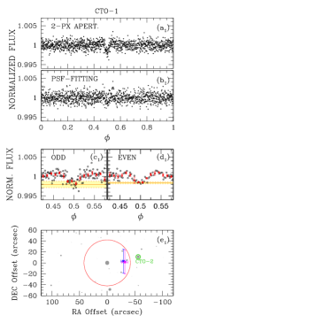
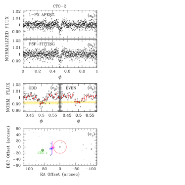
The first two candidates are two close stars at a distance $\delta r\simeq 57.2$ arcsec, and show similar signals in their light curves. The brighter star (Gaia DR2 4689801887175745536, hereafter CTO-1) has $T\sim 12.2$ and, as explained in Sect. 2.5, the best light curve is obtained using the 2-pixel aperture photometry. The fainter star (Gaia DR2 4689813608144062080, hereafter CTO-2) has $T\sim 14.3$, and 1-pixel aperture photometry gives the best result. The two stars present a periodic transit event with period $P\sim 3.982$ d, but different depth: for CTO-1, the transit depth is $\sim 0.2$ % (panel (a₁) of Fig. 8), while for CTO-2 the transit is $\sim 4$ times deeper, as shown in panel (a₂) of Fig. 8.

To verify if the signal belongs to CTO-1 or CTO-2, for both the targets we compared the best-aperture photometry with the PSF-fitting photometry (panels (b) of Fig. 8), that is less affected by contamination problems. As shown in panel (b₁) of Fig. 8, even if the scatter of the PSF-fitting light curve of CTO-1 is similar to that of 2-pixel aperture photometry ($\sigma({\rm PSF})\sim 1060$ ppm versus $\sigma({\rm APER})\sim 970$ ppm), the PSF-fitting photometry shows a less evident transit, with depth $\sim 0.1$%. On the other hand, comparing the PSF-fitting (panel (b₂)) and 1-pixel aperture (panel (a₂)) photometries of CTO-2, it is possible to confirm the presence of the transits in both light curves, with the same depth.

As shown in Fig. 8, we compared the depth of odd (panels (c)) and even (panels (d)) transits, to exclude the hypothesis that the transits events are eclipses of an eclipsing binary. We calculated the mean depth of odd/even transits (orange continuous lines in panels (c)) and its standard deviation (yellow strips): for CTO-1, we found that the odd and even transits have a depth of $2.1\pm 0.8$ mmag and $1.6\pm 0.3$ mmag, respectively; CTO-2 have odd and even transits depth of $8.3\pm 1.9$ mmag and $7.2\pm 1.3$ mmag. For both stars, the depth of odd and even transits overlaps within 1$\times\sigma$.

We analysed the centroid offset using the technique described by Twicken et al. (2018). Briefly, we selected the images corresponding to the in-of-transit events and the images near the transit events (out-of-transit). For each transit, we calculated the mean in- and out-of-transit images, and then we stacked together all the mean in- and out-of-transit images. We calculated the difference image subtracting pixel-by-pixel the in-of-transit stack to the out-of-transit stack. We calculated the photocentres on the out-of-transit and on the difference images. We calculated two offsets: (1) the difference between the centroid obtained from the out-of-transit and the difference images, and (2) the difference between the Gaia DR2 position and the centroid from the difference image. The offset locates the source of the transit signature.

Table 1: Transit parameters for the candidate exoplanet.

PATHOS-1
Gaia DR 2 ID	4702085154340085248
$\alpha_{\rm J2000}$ (∘)	2.87965146
$\delta_{\rm J2000}$ (∘)	$-$70.98693522
$T$ (mag)	15.3
$R_{\star}$ ($R_{\odot}$)	$0.86\pm 0.02$
$M_{\star}$ ($M_{\odot}$)	$0.78\pm 0.02$
$\rho_{\star}\,(\rho_{\odot})$	$1.24_{-0.06}^{+0.07}$
Period (d)	$3.8582_{-0.0014}^{+0.0017}$
$T_{0}$ (BTJD)	$1339.677\pm 0.003$
$R_{\rm p}/R_{\star}$	$0.152_{-0.009}^{+0.011}$
$R_{\rm p}$ ($R_{\rm Jup}$)	$1.27_{-0.07}^{+0.10}$
$a/R_{\star}$	$11.11_{-0.22}^{+0.17}$
$i$ (∘)	$89.2_{-0.5}^{+0.8}$
$T_{14}$ (min)	$181_{-4}^{+5}$
$u1$	$0.42\pm 0.10$
$u2$	$0.18\pm 0.10$

Panels (e) of Fig. 8 shows the out-of-transit centroid analysis for the two stars. In each panel, the target star is centred in (0,0) and the red circle is the photometric aperture used to extract the light curve; in grey are all the sources in the Gaia DR2 catalogue, and magenta and blue crosses are the centroid offsets calculated using the centroids from the out-of-transit image and the position from Gaia DR2, respectively. According to the centroids, the transit events do not occurs on CTO-1 or CTO-2, but to a very faint star ($G>17.2$) between the two candidates.

We searched in literature whether already discovered eclipsing binaries with magnitude $G>17$ are located in that sky regions: Pawlak et al. (2016), in a study of eclipsing binaries in the Magellanic Clouds using OGLE data (Udalski et al. 1992), found an eclipsing binary (OGLE-SMC-ECL-6193) with period $P\sim 7.9733$, so twice the period of the two candidates, $G\sim 17.25$ and located exactly where the centroids are shown in panels (e) of Fig. 8. The depth of the primary eclipses is $\sim 0.3$ magnitudes, while that of the secondary eclipses is $\sim 0.2$ . So, given the differences in magnitudes between the two candidates and the eclipsing binary and the fraction of light of the eclipsing binary that falls within the aperture of the two candidates, we expect an induced transit of depth $\sim 0.1$% and $\sim 1$% for CTO-1 and CTO-2, respectively.

We conclude that the two candidates are false positive generated by the blending with a fainter eclipsing binary located between them.

Figure 10: Panel (a) shows the $G$ versus $G_{\rm BP}-G_{\rm RP}$ CMD: in red are the stars that have high probability to be 47 Tuc members, in green the stars with high probability to belong to the SMC, in grey the field stars of the Milky Way. Panel (b) is the VPD for 47 Tuc, SMC, and Milky Way stars plotted in red, green and grey, respectively. Panel (c) shows the absolute magnitude $M_{G}$ versus $G_{\rm BP}-G_{\rm RP}$ CMD for the Milky Way stars. In all the panels, the position of the candidate exoplanet PATHOS-1 is shown in azure. Panel (d) is the phased light curve of PATHOS-1; in red the best-fit model (see text for details).

3.2.2 A candidate exoplanet: PATHOS-1

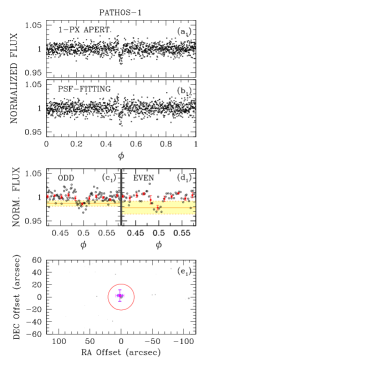
Figure 9 shows the vetting procedure for the candidate transiting exoplanet PATHOS-1 ($T\sim 15.3$, $P\sim 3.86$ d). The comparison between the best photometry (1-pixel aperture, panel (a₁)) and the PSF-fitting photometry shows that it is possible to identify the transit events in both of the light curves. Comparing the odd ($1.3\pm 0.6$ %) and even ($2.2\pm 1.3$ %) transit events (panels (c₁) and (d₁)) we found that the depths are compatible within 1$\times\sigma$. From the analysis of out-of-transit centroids (panel (e₁) of Fig. 9), we confirm that the transit events occur on PATHOS-1.

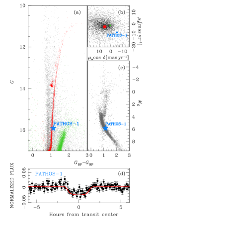
PATHOS-1 is a field star located on the main sequence (MS) of the Galaxy (see panels (a), (b), and (c) of Fig. 10).

We extracted transit parameters using a modified version of the code used by Borsato et al. (2019) and Benatti et al. (2019). It selects a portion of the light-curve around each transit of about $\pm 2\times T_{14}$ ($T_{14}$ is the duration of the transit from the TLS) from the linear ephemeris determined with TLS. This code models the transit with the batman-package (Kreidberg 2015) and computes the posterior distribution with emcee (affine invariant Markov-Chain Monte Carlo sampler, Foreman-Mackey et al. 2013).

The code fits as common parameters the stellar density $\rho_{\star}$ (in Solar unit), the base-2 logarithm of the period of the planet ($\log_{2}P$), the radii ratio ($k=R_{\mathrm{p}}/R_{\star}$), the impact parameter ($b$), the quadratic limb darkening (LD) parameters, $q_{1}$ and $q_{2}$, as proposed by Kipping (2013), a base-2 logarithm of a jitter term ($\log_{2}\sigma_{j}$), the reference transit times ($T_{0}$). For each transit it fits a detrending polynomial of third order (coefficients $c_{0}$, $c_{1}$, $c_{2}$) and the time of the centre of the transit ($TT$). It this way it computes simultaneously each transit time ($TT$) and the linear ephemeris (given by the period and $T_{0}$). We fixed the eccentricity $e$ to 0 and the argument of the pericenter $\omega$ to 90 deg. We used uniform-uninformative priors within conservative boundaries for all the parameters, but Gaussian priors for the stellar density and LD parameters. The prior for the density has been computed from the stellar radius ($R_{\star}$) and mass ($M_{\star}$); from the Gaia DR2 catalogue the star has $R_{\star}=0.86\pm 0.02\,R_{\odot}$ and, using mass-luminosity relation $L\propto M^{3.5}$, we found $M_{\star}=0.78\pm 0.02\,M_{\odot}$. The quadratic LD parameters have been determined from the Claret (2018) table for $T_{\rm eff}=4985\pm 59$ K (from Gaia DR2) and we adopted priors with a Gaussina conservative error of about 0.1 for both the parameters.

We run emcee with 72 walkers and for 20 000 steps. We removed the first 2000 steps as burn-in (checked visually the convergence of the chains) and we used a pessimistic thinning factor of 100. From the posterior distribution we computed the physical posteriors and computed the uncertainties as the high density interval (HDI) at $68\%$ ($1\sigma$ equivalent). We computed the median of the physical posterior distribution as the best-fit transit parameters (reduced $\chi^{2}\sim 0.92$). We found that the period of the candidate exoplanet is $P\sim 3.8582$ d and $k\sim 0.152$, i.e., $R_{\mathrm{p}}\sim 1.27\,R_{\mathrm{Jup}}$. Table 1 gives all the physical parameters with errors.

Panel (d) of Fig. 10 shows the phased light curve and, over-imposed in red, the best fitting model.

Figure 11: Procedure adopted for the selection of candidate variable stars. Panels (a), (b), and (c) show the selection in the SNR versus Period plane for the GLS, AoV, and BLS periodograms, respectively: in orange are the stars that have high probability to be variables. Panels (d) and (e) are the VPD and the $G$ versus $G_{\rm BP}-G_{\rm RP}$ CMD, respectively: in blue, red, and green are the candidate variable stars that belong to field, 47 Tuc, and SMC, respectively. Panels (f) are some examples of light curves of stars with high probability to be variables: the light curves are colour-coded as in panel (d) and (e).

Figure 12: Light curves of eclipsing binaries found in the field analysed in this work. Light curves are colour-coded as in Fig. 11.

Table 2: List of eclipsing binaries

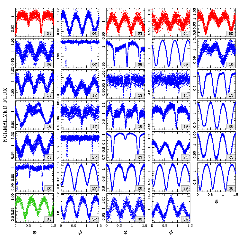
# EB	$\alpha$(J2000)	$\delta$(J2000)	Gaia DR 2 ID	$T$	$G$	$G_{\rm BP}$	$G_{\rm RP}$	$\mu_{\alpha}\cos\delta$	$\mu_{\delta}$	P	Note	Ref.
	(∘)	(∘)						(mas yr-1)	(mas yr-1)	(d)
01	6.537000594	-72.11708689	4689629611756844672	15.65	15.84	15.95	15.59	5.267	-1.957	1.150726	V46, 0063	(1,2)
02	5.697991131	-72.22145320	4689625041910756480	15.11	15.53	15.84	15.04	11.575	-1.031	0.278849	V50	(1)
03	6.543979192	-72.18550401	4689628203007617792	16.17	16.46	16.52	15.98	5.660	-2.563	0.378792	V45, 6257	(1,2)
04	5.825314808	-72.31158497	4689619853590073216	13.33	13.88	14.34	13.26	5.802	-2.943	0.383336	V49	(1)
05	6.679190520	-72.25576887	4689579961931616640	16.38	16.72	16.93	16.29	5.911	-2.183	0.446193	V53, 6261	(1,2)
06	6.749464138	-71.91938968	4689646757262208000	15.43	15.88	16.01	15.16	7.993	2.603	0.347537	KalE1	(1)
07	5.413085792	-72.52089953	4689547010942141056	13.47	14.00	14.42	13.41	9.254	-10.723	5.227904
08	6.355276472	-72.54985787	4689552783378799744	13.75	14.41	14.96	13.66	12.478	6.540	0.677519	0057	(2)
09	4.340046990	-71.91583531	4689821167286415744	9.74	10.02	10.25	9.71	29.282	-10.217	0.594934	AQ Tuc	(3)
10	3.926140119	-72.40455559	4689606693809057920	12.52	12.85	13.08	12.47	12.182	0.874	4.183775
11	5.617000506	-71.35597297	4689919401777839872	15.25	15.57	15.80	15.19	2.629	-2.465	0.271553	6237	(2)
12	4.438502576	-71.47351863	4689892051426793088	15.93	16.64	17.27	15.85	1.607	2.576	0.301928	6202	(2)
13	8.383993384	-72.44371408	4689170393848047616	16.37	16.34	16.29	16.28	-2.151	-0.490	9.700781	0190	(2)
14	8.667676514	-72.42093551	4689175444729490176	16.09	16.58	16.96	16.02	7.916	-2.849	6.348956	6320	(2)
15	3.233508991	-72.31701594	4689705065728365952	13.87	14.58	15.23	13.80	14.594	-11.702	6.221432
16	8.890463344	-72.00424710	4689948607555229440	13.31	14.00	14.62	13.25	21.512	-7.481	8.311906
17	9.001923031	-72.13692603	4689195235938665984	16.49	16.95	17.30	16.42	10.471	-0.916	2.195023
18	3.106567298	-71.63696759	4701807184057132544	15.34	16.07	16.76	15.26	19.053	-9.645	0.797952
19	7.236826679	-73.04733569	4688719937672536576	15.52	16.02	16.39	15.44	9.457	1.928	0.887469	0110	(2)
20	6.095619143	-71.04839847	4701937201307042304	10.84	11.28	11.58	10.75	-9.681	-32.364	0.337970
21	8.348316851	-71.26629784	4690231525639747072	5.84	6.04	6.22	5.83	73.596	-12.372	7.108649	Theta Tuc	(3)
22	4.674966177	-71.02474137	4701931566310065280	16.15	16.73	17.19	16.06	17.406	1.644	3.666514	6209	(2)
23	2.505425028	-71.58902403	4701817938655245568	10.51	10.77	10.95	10.48	2.737	3.244	2.727260
24	9.268095200	-71.43438559	4690047048205684736	15.86	16.11	16.27	15.80	4.118	4.035	0.462172	0301	(2)
25	2.113365648	-72.31207417	4689760969022718720	13.08	13.49	13.79	13.02	-0.194	0.552	0.330047	6174	(2)
26	4.262175365	-70.99149906	4701976680646546688	11.58	12.16	12.65	11.52	15.144	-10.681	1.406333
27	2.826367562	-71.30014165	4701877209203898368	13.83	14.37	14.83	13.76	-12.364	-6.930	0.269175	6181
28	4.266066198	-70.91246927	4701989595612092416	15.96	16.92	18.00	15.88	6.717	-7.449	0.302563
29	5.461765066	-70.77851842	4702006058222771072	12.30	12.82	13.27	12.25	11.954	-7.653	0.271736
30	2.157617319	-71.48742290	4701865698691623680	13.59	14.03	14.39	13.54	2.934	1.175	0.305206	6175	(2)
31	7.088826924	-73.39119841	4688521407109977344	15.68	16.48	17.28	15.61	0.379	-1.267	1.705885
32	5.850347702	-73.53212906	4688493335202967680	16.44	16.84	17.10	16.34	0.714	-4.793	0.385427	0024	(2)
33	2.534043926	-71.11817683	4701889887947453824	15.58	16.01	16.34	15.51	19.158	-8.877	0.177335
34	3.200471157	-73.29941528	4688666370837766144	14.62	14.92	15.12	14.56	2.890	-10.635	1.917045
References (1) Clement et al. (2001, updated to 2017); (2) Pawlak et al. (2016); (3) Samus’ et al. (2017)

4 Variable stars

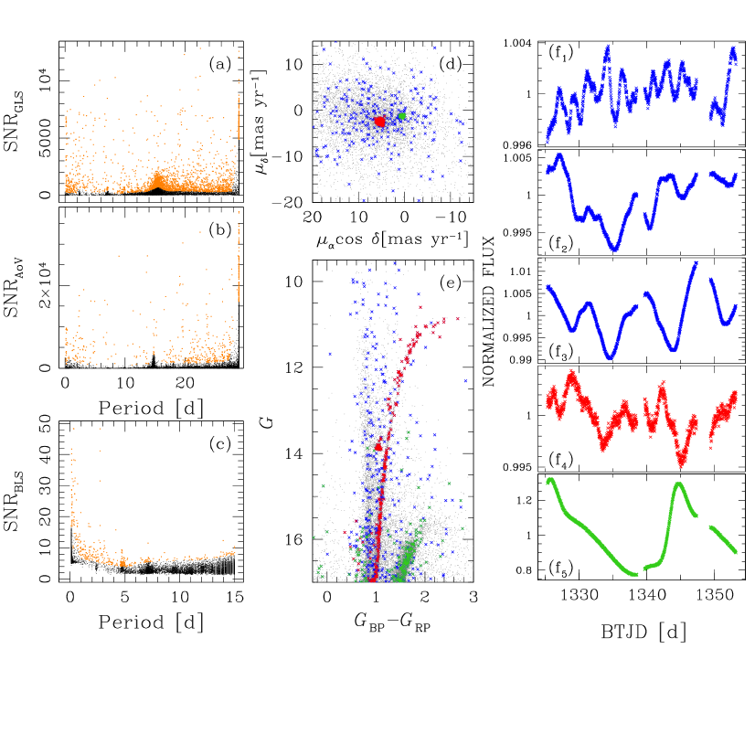
Variable star detection has been performed using three different algorithms: the Generalized Lomb-Scargle (GLS) periodogram (Zechmeister & Kürster 2009), the Analysis of Variance (AoV) periodogram (Schwarzenberg-Czerny 1989), and the BLS periodogram. The procedure is illustrated in Fig. 11. We isolated the candidate variable stars using the Signal-to-Noise Ratio (SNR) parameter and adopting the procedure described in Nardiello et al. (2015): first, we produced the histograms of the detected periods for all the light curves and suppressed the spikes due to systematic effects in the light curves. We divided the SNR distributions in bins of period $\delta P=1$ d and we computed the 3.5$\sigma$-clipped mean and standard deviation values of the SNR within each period interval. We interpolated the points 4$\sigma$ above the mean values with a spline and selected all the stars above this line (orange points in panels (a), (b), and (c) of Fig. 11). The number of candidate variable stars so selected are 2446 and 561 according the GLS and AoV algorithms, respectively. The variables identified by both the techniques are 502. The number of variable sources found with BLS periodogram is 391. We used a routine of VARTOOLS (Hartman & Bakos 2016) to exclude the sources that show variability because blended with a real variable star. After excluding blends and after a visual inspection, we identified 34 eclipsing binaries. Positions of the candidate variables in the VPD and CMD are plotted in blue (field stars), red (47 Tuc members), and green (SMC stars) in panels (d) and (e) of Fig. 11, respectively. Panels (f) show some examples of variable stars, colour-coded as in panels (d) and (e). The magnitude of these stars spans from $T\sim 7.4$ to $T\sim 13.4$.

4.1 Eclipsing Binaries

We detected 34 eclipsing binaries. Their phased light curves are shown in Fig. 12 colour-coded as the variables in Fig. 11. Among the detected eclipsing binaries, 4 of them have a high probability to be 47 Tuc members (in red), one is a star in the SMC (in green), and the other 28 stars belong to the Galactic field (in blue). In Table 2 we listed the 34 eclipsing binaries. We cross-identified our list of eclipsing binaries with other catalogues in literature. We found 6 stars in common with the catalogue by Clement et al. (2001, updated to 2017), 13 listed also in the catalogue of eclipsing binaries based on OGLE data (Pawlak et al. 2016), and two in the GCVS catalogue (Samus’ et al. 2017). The period distribution of the detected eclipsing binaries is peaked at $\sim$0.3-0.4 d, and $\sim 58$ % of stars have P$<1$ d and are contact binaries.

4.2 RGB and AGB stars of 47 Tuc

We analysed the RGB stars members of 47 Tuc, that we flagged as candidate variable, to find their variability periods. To minimise the effects of the blends, we excluded from the analysis the RGB stars located at a distance $<7.5$ arcmin from the cluster centre. We also excluded all the stars that are blends, by comparing their light curves (and the periods found by GLS/AoV) with those of the neighbours located at a distance of 100 arcsec. After these selections, we saved 54 RGB stars with a good light curve. A sample of these light curves is shown in panels (a) of Fig. 13, while in panel (b) we show their position (red points) on the $T$ versus $G_{\rm BP}-G_{\rm RP}$ CMD. We re-extracted the GLS periodograms for these light curves, but in this second iteration we looked for periods between 0.1 and 150 days. We listed the 54 RGB stars, their astro-photometric properties and their periods in Table 3.

In this paper we extend the work by Lebzelter et al. (2005): they analysed the long period, pulsating stars located on the tip of the RGB in the Period-Luminosity (PL) plan. Because of the uncertainties on their photometric series, their study was limited to stars with $V\lesssim 12$. Thanks to the high quality of our light curves, we are able to extend the PL distribution to fainter magnitudes ($T\sim 15.1$). Panel (c) of Fig. 13 shows the relation between $T$ magnitude and the period for the RGB stars analysed by Lebzelter et al. (2005, azure squares) and by us (red points): the two distributions are superimposed. In the range $9.5\lesssim T\lesssim 12.0$, the period is proportional to the luminosity of the stars. In the range $12.0\lesssim T\lesssim 15.5$ we found the unexpected result that the period is inversely proportional to the luminosity. For completeness, we show the relation Period-Colour (PC) in panel (d) of Fig. 13: for $(G_{\rm BP}-G_{\rm RP})\gtrsim 1.5$ the period grows with the colour, while for $(G_{\rm BP}-G_{\rm RP})\lesssim 1.5$ the period decreases with the colour.

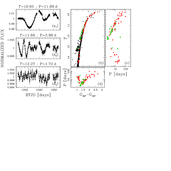
We did the same analysis with the asymptotic giant-branch (AGB) stars members of 47 Tuc. We found 24 AGB variable stars with good light curves; they are listed in Table 4. We derived the period by using the GLS periodogram and looking for periods between 0.1 and 150 days. Finally we analysed the PL and PC distributions. Figure 14 summarises the results. Panels (c) and (d) show that the PL and PC distributions for AGB (in green) and RGB (in red) stars are superimposed.

A detailed analysis of the PL/PC distributions for AGB and RGB stars in globular clusters is beyond the scope of this work and might be the subject of a future analysis based on our released light curves.

Figure 13: Analysis of RGB stars. Panels (a₁)-(a₈) show a sample of light curves of RGB stars, ordered by magnitude. Panel (b) shows $T$ versus $G_{\rm BP}-G_{\rm RP}$ CMD; panels (c) and (d) are the PL and the PC relations. In panels (b), (c), and (d) azure squares are determined by Lebzelter et al. (2005), red points are obtained in this work.

Table 3: List of the analysed RGB stars in 47 Tuc

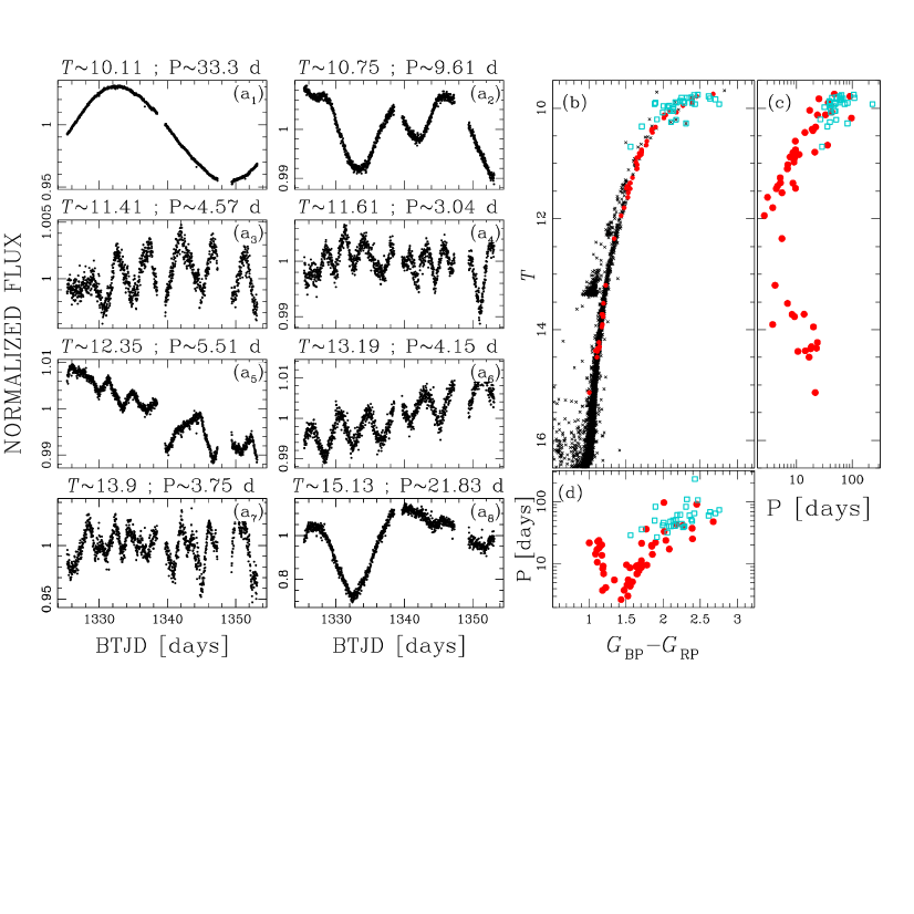
$\alpha$(J2000)	$\delta$(J2000)	Gaia DR 2 ID	$T$	$G$	$G_{\rm BP}$	$G_{\rm RP}$	P	$\sigma_{P}$
(∘)	(∘)						(d)	(d)
RGB
6.42920058	$-72.06821514$	4689627069134206080	13.72	14.32	14.82	13.65	13.76	0.10
6.43662601	$-72.08778119$	4689627000414752896	14.31	14.89	15.38	14.23	18.62	0.26
5.66859934	$-72.14857213$	4689637407107299840	10.97	11.76	12.55	10.91	9.08	0.13
6.01883235	$-71.95310074$	4689644730042501760	10.60	11.43	12.32	10.54	9.59	0.06
6.12140329	$-72.20647551$	4689623010398337408	13.95	14.54	15.05	13.88	20.27	0.21
5.64847070	$-72.02281411$	4689642698537939328	13.72	14.32	14.84	13.65	8.37	0.11
6.43320055	$-72.11410571$	4689626725536883328	9.95	10.96	12.17	9.90	41.55	—
6.44980872	$-72.08972115$	4689626794256322048	14.39	14.96	15.42	14.31	10.65	0.17
6.45352017	$-72.08855492$	4689626794256321024	14.35	14.92	15.36	14.23	18.00	0.18
6.41109649	$-72.01835333$	4689639919678548736	11.41	12.15	12.82	11.31	4.58	0.02
5.59606753	$-72.11807831$	4689638373492005888	10.75	11.56	12.40	10.69	9.66	0.14
6.37838253	$-71.99910431$	4689640194556564224	14.38	14.94	15.39	14.30	14.44	0.12
5.57456597	$-72.10343371$	4689638442211439872	10.12	11.04	12.08	10.07	33.31	—
6.35701402	$-72.17760343$	4689623289563167360	10.12	11.05	12.11	10.07	23.89	0.34
6.49858087	$-72.07526996$	4689632875931941888	11.02	11.81	12.61	10.96	7.02	0.07
6.48973686	$-72.13133662$	4689629371238695552	11.61	12.35	13.07	11.55	3.04	0.01
6.51160277	$-72.05507897$	4689632974708827776	13.20	13.82	14.36	13.13	4.16	0.03
6.34367313	$-72.19870524$	4689622460621134720	11.35	12.11	12.85	11.29	8.67	0.15
5.83524393	$-71.93883381$	4689831200329811840	14.50	15.06	15.53	14.43	16.91	0.24
5.52387023	$-72.06572626$	4689618273040536704	10.67	11.50	12.38	10.61	36.33	—
5.64934543	$-72.18648647$	4689625282428885120	9.78	10.84	12.21	9.76	91.28	—
6.03188484	$-71.92610741$	4689645004920347264	15.14	15.65	16.07	15.06	21.84	0.38
6.21701197	$-71.93645739$	4689644420804776960	9.90	10.94	12.25	9.865	37.41	—
6.21656039	$-72.22729200$	4689622052612663680	14.23	14.81	15.29	14.16	23.82	0.42
6.31562558	$-72.21235971$	4689622430569760640	10.89	11.68	12.48	10.83	9.34	0.07
5.52469338	$-72.13027478$	4689614901478662272	10.40	11.27	12.19	10.34	19.83	0.12
6.05234523	$-71.92107173$	4689645107999550720	11.80	12.52	13.21	11.73	3.77	0.03
6.45510154	$-72.19421879$	4689622396209979136	14.34	14.91	15.37	14.25	23.03	1.14
6.28343260	$-71.92632578$	4689644352084823936	13.77	14.37	14.89	13.70	9.25	0.09
5.98279786	$-71.90490959$	4689832712158218880	12.36	13.02	13.64	12.29	5.51	0.05
6.51617594	$-71.97513601$	4689645898275596288	13.53	14.13	14.66	13.46	6.95	0.06
5.71571955	$-72.24380077$	4689624212967816064	11.09	11.88	12.67	11.02	6.96	0.05
6.09369763	$-71.89129882$	4689832849597140096	9.83	10.87	12.19	9.79	25.36	2.28
6.40041875	$-72.23750838$	4689575289007212416	11.45	12.18	12.89	11.38	9.65	0.08
5.91328145	$-72.27775711$	4689620334626390784	10.38	11.24	12.17	10.32	19.23	0.03
5.39619011	$-71.99971800$	4689807354671547648	10.04	10.98	12.08	9.99	17.35	0.28
5.57486258	$-72.26169193$	4689600680854700288	10.79	11.61	12.44	10.73	21.47	0.21
5.68279610	$-71.87548264$	4689835082980178304	11.94	12.65	13.31	11.88	2.66	0.01
6.76144736	$-72.01953661$	4689633460047351296	11.35	12.10	12.84	11.28	5.17	0.03
6.51675254	$-71.88983356$	4689650330681896320	10.34	11.22	12.18	10.28	22.14	0.05
5.18998805	$-72.07752865$	4689806457019852160	10.82	11.62	12.43	10.76	9.63	0.06
6.25387493	$-72.34392027$	4689573364861989760	11.10	11.89	12.68	11.04	6.88	0.04
5.31194405	$-72.25063322$	4689612981641053696	10.76	11.57	12.41	10.70	9.61	0.06
5.22378507	$-72.22670400$	4689613183491785856	11.45	12.21	12.95	11.39	4.38	0.02
5.97192517	$-71.78663649$	4689837419442795648	10.8	11.61	12.44	10.74	8.72	0.05
5.87516442	$-72.37674822$	4689572677667393664	9.74	10.86	12.39	9.71	47.97	—
6.61872853	$-71.83689944$	4689651086596023040	11.26	12.02	12.78	11.19	5.13	0.03
5.68086357	$-71.77517546$	4689848655076717440	11.53	12.27	12.99	11.47	5.53	0.05
7.06600513	$-72.15084334$	4689582435832666752	10.07	11.05	12.18	10.00	43.35	—
6.61344377	$-71.79558420$	4689652117388263296	10.88	11.68	12.49	10.82	7.67	0.08
6.73945779	$-71.82054282$	4689651151009833728	10.84	11.65	12.48	10.77	11.22	0.15
5.41339391	$-72.41406304$	4689595831823970304	10.18	11.10	12.13	10.12	97.15	—
6.62113569	$-71.66616431$	4689844287094705408	13.91	14.51	15.03	13.84	3.76	0.01
6.79559874	$-72.51910046$	4689558074778482304	10.44	11.30	12.24	10.38	14.25	0.05

Table 4: List of the analysed AGB stars in 47 Tuc

$\alpha$(J2000)	$\delta$(J2000)	Gaia DR 2 ID	$T$	$G$	$G_{\rm BP}$	$G_{\rm RP}$	P	$\sigma_{P}$
(∘)	(∘)						(d)	(d)
AGB
6.01688895	-71.94061171	4689644798761947520	10.65	11.47	12.30	10.60	11.89	0.25
5.55209154	-72.09583082	4689641392838717568	12.10	12.73	13.29	12.04	30.93	0.08
6.47697044	-72.03029288	4689633975443492736	11.39	12.10	12.78	11.33	5.15	0.04
5.54159063	-72.05543971	4689642496660354048	11.45	12.18	12.88	11.39	4.74	0.07
5.96855292	-71.93058778	4689645039280106624	13.17	13.71	14.17	13.10	17.40	0.19
6.34863462	-72.20215239	4689622460621136256	11.83	12.50	13.11	11.77	3.14	0.03
5.84093194	-71.93252052	4689831264750937344	11.40	12.14	12.85	11.35	5.70	0.06
6.39289277	-71.95979283	4689641083606519168	11.64	12.32	12.96	11.58	3.78	0.04
5.47065091	-72.14455881	4689614867118928384	11.38	12.11	12.80	11.33	4.59	0.03
5.81541011	-71.89896796	4689832192474832000	11.11	11.86	12.59	11.06	4.00	0.04
6.34588623	-71.91017173	4689644592602980608	11.33	12.07	12.78	11.27	2.85	0.03
5.39536304	-72.14050345	4689617792004292096	12.06	12.71	13.29	12.00	1.87	0.02
5.50575090	-72.22177206	4689601746006553344	11.31	12.05	12.76	11.25	10.75	0.17
6.76078109	-72.02121070	4689633253888922624	13.10	13.67	14.15	13.04	4.88	0.02
6.59880135	-71.89197969	4689647405798359936	12.26	12.91	13.49	12.19	2.27	0.02
6.72736160	-72.22744307	4689580271169229824	12.27	12.93	13.52	12.22	1.87	0.01
5.55421378	-72.30091451	4689600332949678848	10.91	11.69	12.47	10.85	9.64	0.08
6.43414368	-72.31488155	4689573914617758336	12.15	12.80	13.40	12.09	1.89	0.01
6.95294326	-71.95535448	4689635178034205056	11.81	12.48	13.11	11.75	3.33	0.02
5.25552963	-72.31604682	4689600852653460352	11.59	12.28	12.92	11.54	4.64	0.02
7.13714170	-72.10676444	4689583294826108160	12.16	12.81	13.38	12.11	1.88	0.01
5.41790367	-72.38729162	4689596111009591936	12.27	12.91	13.47	12.21	1.72	0.01
5.30446552	-71.64086650	4689877654695832704	11.66	12.35	12.99	11.60	3.98	0.02
4.10826661	-72.35587640	4689607995176575488	11.53	12.24	12.92	11.47	4.66	0.08

Figure 14: Analysis of AGB stars. Panels (a₁)-(a₃) show a sample of light curves of AGB stars, ordered by magnitude. Panel (b) shows $T$ versus $G_{\rm BP}-G_{\rm RP}$ CMD; panel (c) and (d) the PL and the PC relations. In panels (b), (c), and (d) red circles and green starred points are RGB and AGB stars, respectively.

Figure 15: Comparison between the raw light curves extracted with the PATHOS pipeline (in blue, left panels) and the eleanor pipeline (in red, middle panels). Right panels show the finding charts of the target stars, obtained by using the Gaia DR2 data: in red the size of the aperture used for the extraction of the light curves. The light curves are sorted by magnitude.

5 Comparison with other pipelines

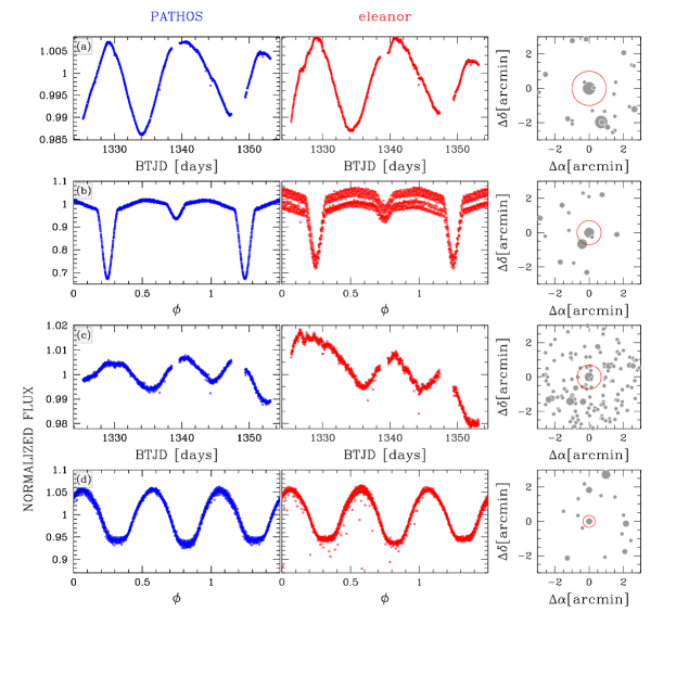
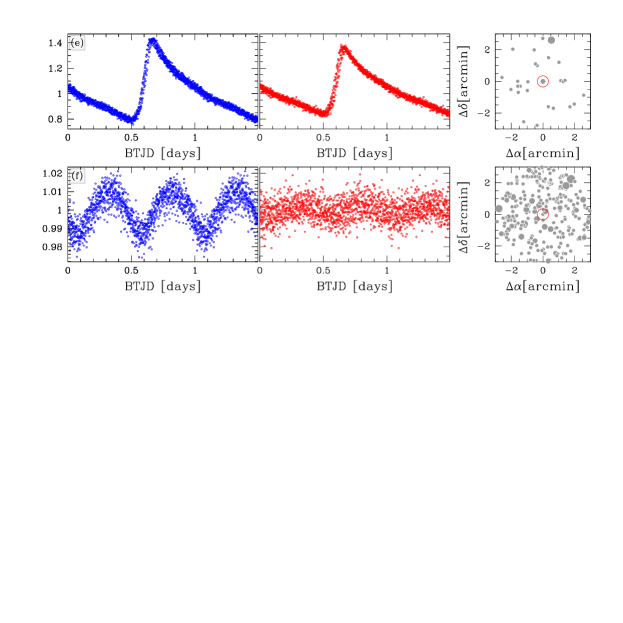
At present, the most advanced pipeline aimed at the extraction of any kind of light curve from FFIs is eleanor (Feinstein et al. 2019). In this section we compare the quality of our photometry with that obtained by eleanor, highlighting the importance of neighbour subtraction when we consider crowded environments. Figure 15 shows six different raw light curves of stars with different luminosities and located in environments characterised by different levels of crowding. Panels on the right show that the contamination by neighbour stars in the cases (a) (Gaia DR2 4689720939927488768, $T\sim 7.7$), (d) (Gaia DR2 4689760969022718720, $T\sim 13.1$), and (e) (Gaia DR2 4689953108681026304, $T\sim 15.6$ ) is low, and the raw light curves output of the PATHOS pipeline (left panels, in blue) and eleanor pipeline (middle panels, in red) are similar. The light curves were extracted by using the same photometric apertures. In crowded environments, the dilution and contamination by neighbour stars affect the quality of the light curves extracted with eleanor. In the case (b) (Gaia DR2 4701817938655245568, $T\sim 10.5$) the bright neighbour star dilutes the light of the target star during the eclipses, with the result that the observed depth of the eclipses is lower. This effect is important especially in the light curve analysis of candidate transiting exoplanets: without considering the dilution effects due to neighbour stars, the radius of the candidate exoplanet would be underestimated. In the cases (c) (Gaia DR2 4689837419442795648, $T\sim 10.8$) and (f) (Gaia DR2 4689619853580301824, $T\sim 15.9$) the presence of many neighbour stars strongly affects the shape and the quality of the light curve of the target star; in particular, in the case (f) the variability of the target star is significantly diluted by the light of the neighbour stars.

6 The data release

We publicly release all the light curves extracted in this work. The light curves will be available in the Mikulski Archive for Space Telescopes (MAST) as a High Level Science Product (HLSP) via https://doi.org/10.17909/t9-es7m-vw14. Each light curve contains the epoch in BTJD, the 5 extracted photometries (PSF-fitting, 1-pixel, 2-pixel, 3-pixel, 4-pixel aperture), the value of the local sky, the position $(x,y)$ on the image, and the data quality flag (see Sect. 9 of the TESS Science Data Products Description Document, for details). Light curves are both in ascii and fits format, which header contains information on the star (from the Gaia DR2 catalogue) and on its observations.

7 Summary

In this work we presented our PSF-based approach, applied for the first time to TESS FFIs, in order to extract light curves of stars in a crowded field centred on 47 Tuc. The pipeline presented in this pilot work is essential for the success of the PATHOS project, whose main scope is the analysis of high-precision light curves of stellar cluster members, in order to find candidate exoplanets orbiting bright cluster stars and variable stars.

Discovering and characterising exoplanets in stellar clusters (especially open clusters and young associations) represent an important ingredient to understand how exoplanet systems have formed and evolved. At variance with what happens for most Galactic field stars, cluster star parameters (such as age, mass, and chemical composition) are generally well determined with high accuracy. This allows us to correlate stellar parameters (such as stellar mass) with exoplanet characteristics. Furthermore, hundreds of stellar clusters populate the Milky Way (Cantat-Gaudin et al. 2016), having ages that span from few tens Myrs to $\sim 10$ Gyrs (Bossini et al. 2019) and showing a wide variety of chemical compositions. Combining pieces of information on stellar clusters with exoplanet properties (and with the rate of exoplanets in stellar clusters), it will be possible to understand how ages of stars, and the environment in which they are embedded, have affected the formation and evolution of exoplanets.

In this pilot project we have extracted, corrected, and analysed the light curves of 16641 stars in a field containing the globular cluster 47 Tuc. These stars belong either to 47 Tuc, or the Milky Way, or the SMC. We took advantage of the Gaia DR2 catalogue to extract not only astro-photometric data of stars located in this region, but also, when possible, stellar parameters. We searched for transit signals among the extracted light curves and we found and characterised a candidate transiting exoplanet orbiting a MS field star. This candidate exoplanet, named PATHOS-1, is not in the list of TESS Objects of Interest (TOI) and is a new discovery. No candidate transiting exoplanets have been found around bright RGB stars of 47 Tuc; given the nature of RGB stars, the probability of finding exoplanets orbiting them and having periods $<27$ days, is low. We also searched for variables among the stars in the analysed field. We analysed the 34 eclipsing binaries in the field and the relations PL and PC for the RGB and AGB stars members of 47 Tuc. We found that the period of variability for AGB and RGB stars is proportional to the luminosity above the mean magnitude of the RGB bump, but we found also that below the RGB bump the period decreases as the stellar brightness increases.

The raw and corrected light curves will be uploaded on the MAST archive as HLSP. In this way, they will always be available to the astronomical community for any scientific goal.

References

- Aigrain et al. (2016) Aigrain S., Parviainen H., Pope B. J. S., 2016, MNRAS, 459, 2408
- Anderson et al. (2006) Anderson J., Bedin L. R., Piotto G., Yadav R. S., Bellini A., 2006, A&A, 454, 1029
- Armstrong et al. (2016) Armstrong D. J., et al., 2016, MNRAS, 456, 2260
- Baglin et al. (2006) Baglin A., et al., 2006, in 36th COSPAR Scientific Assembly. p. 3749
- Barros et al. (2016) Barros S. C. C., Demangeon O., Deleuil M., 2016, A&A, 594, A100
- Benatti et al. (2019) Benatti S., et al., 2019, arXiv e-prints, p. arXiv:1904.01591
- Bertin et al. (2002) Bertin E., Mellier Y., Radovich M., Missonnier G., Didelon P., Morin B., 2002, in Bohlender D. A., Durand D., Handley T. H., eds, Astronomical Society of the Pacific Conference Series Vol. 281, Astronomical Data Analysis Software and Systems XI. p. 228
- Borsato et al. (2019) Borsato L., et al., 2019, MNRAS, 484, 3233
- Borucki et al. (2010) Borucki W. J., et al., 2010, Science, 327, 977
- Bossini et al. (2019) Bossini D., et al., 2019, A&A, 623, A108
- Brucalassi et al. (2014) Brucalassi A., et al., 2014, A&A, 561, L9
- Brucalassi et al. (2017) Brucalassi A., et al., 2017, A&A, 603, A85
- Cantat-Gaudin et al. (2016) Cantat-Gaudin T., Donati P., Vallenari A., Sordo R., Bragaglia A., Magrini L., 2016, A&A, 588, A120
- Claret (2018) Claret A., 2018, A&A, 618, A20
- Clement et al. (2001) Clement C. M., et al., 2001, AJ, 122, 2587
- Feinstein et al. (2019) Feinstein A. D., et al., 2019, PASP, 131, 094502
- Foreman-Mackey et al. (2013) Foreman-Mackey D., Hogg D. W., Lang D., Goodman J., 2013, PASP, 125, 306
- Gaia Collaboration et al. (2018) Gaia Collaboration et al., 2018, A&A, 616, A1
- Gilliland et al. (2011) Gilliland R. L., et al., 2011, ApJS, 197, 6
- Gilliland et al. (2015) Gilliland R. L., Chaplin W. J., Jenkins J. M., Ramsey L. W., Smith J. C., 2015, AJ, 150, 133
- Goldsbury et al. (2010) Goldsbury R., Richer H. B., Anderson J., Dotter A., Sarajedini A., Woodley K., 2010, AJ, 140, 1830
- Greisen & Calabretta (2002) Greisen E. W., Calabretta M. R., 2002, A&A, 395, 1061
- Hartman & Bakos (2016) Hartman J. D., Bakos G. Á., 2016, Astronomy and Computing, 17, 1
- Hippke & Heller (2019) Hippke M., Heller R., 2019, A&A, 623, A39
- Howell et al. (2014) Howell S. B., et al., 2014, PASP, 126, 398
- Kipping (2013) Kipping D. M., 2013, MNRAS, 435, 2152
- Kovács et al. (2002) Kovács G., Zucker S., Mazeh T., 2002, A&A, 391, 369
- Kreidberg (2015) Kreidberg L., 2015, PASP, 127, 1161
- Lang et al. (2010) Lang D., Hogg D. W., Mierle K., Blanton M., Roweis S., 2010, AJ, 139, 1782
- Lebzelter et al. (2005) Lebzelter T., Wood P. R., Hinkle K. H., Joyce R. R., Fekel F. C., 2005, A&A, 432, 207
- Libralato et al. (2016a) Libralato M., Bedin L. R., Nardiello D., Piotto G., 2016a, MNRAS, 456, 1137
- Libralato et al. (2016b) Libralato M., et al., 2016b, MNRAS, 463, 1780
- Malavolta et al. (2016) Malavolta L., et al., 2016, A&A, 588, A118
- Mann et al. (2018) Mann A. W., et al., 2018, AJ, 155, 4
- Moré et al. (1980) Moré J. J., Garbow B. S., Hillstrom K. E., 1980, Technical Report ANL-80-74, User guide for MINPACK-1. Argonne Nat. Lab., Argonne, IL
- Nardiello et al. (2015) Nardiello D., et al., 2015, MNRAS, 447, 3536
- Nardiello et al. (2016a) Nardiello D., Libralato M., Bedin L. R., Piotto G., Ochner P., Cunial A., Borsato L., Granata V., 2016a, MNRAS, 455, 2337
- Nardiello et al. (2016b) Nardiello D., Libralato M., Bedin L. R., Piotto G., Borsato L., Granata V., Malavolta L., Nascimbeni V., 2016b, MNRAS, 463, 1831
- Pál et al. (2018) Pál A., Molnár L., Kiss C., 2018, PASP, 130, 114503
- Pawlak et al. (2016) Pawlak M., et al., 2016, Acta Astron., 66, 421
- Pollacco et al. (2006) Pollacco D. L., et al., 2006, PASP, 118, 1407
- Quinn et al. (2012) Quinn S. N., et al., 2012, ApJ, 756, L33
- Quinn et al. (2014) Quinn S. N., et al., 2014, ApJ, 787, 27
- Ricker et al. (2015) Ricker G. R., et al., 2015, Journal of Astronomical Telescopes, Instruments, and Systems, 1, 014003
- Riess et al. (2018) Riess A. G., et al., 2018, ApJ, 861, 126
- Samus’ et al. (2017) Samus’ N. N., Kazarovets E. V., Durlevich O. V., Kireeva N. N., Pastukhova E. N., 2017, Astronomy Reports, 61, 80
- Schwarzenberg-Czerny (1989) Schwarzenberg-Czerny A., 1989, MNRAS, 241, 153
- Shupe et al. (2005) Shupe D. L., Moshir M., Li J., Makovoz D., Narron R., Hook R. N., 2005, in Shopbell P., Britton M., Ebert R., eds, Astronomical Society of the Pacific Conference Series Vol. 347, Astronomical Data Analysis Software and Systems XIV. p. 491
- Soares-Furtado et al. (2017) Soares-Furtado M., Hartman J. D., Bakos G. Á., Huang C. X., Penev K., Bhatti W., 2017, PASP, 129, 044501
- Tange (2011) Tange O., 2011, ;login: The USENIX Magazine, 36, 42
- Twicken et al. (2018) Twicken J. D., et al., 2018, PASP, 130, 064502
- Udalski et al. (1992) Udalski A., Szymanski M., Kaluzny J., Kubiak M., Mateo M., 1992, Acta Astron., 42, 253
- Vallely et al. (2019) Vallely P. J., et al., 2019, arXiv e-prints, p. arXiv:1903.08665
- Van Cleve et al. (2016) Van Cleve J. E., et al., 2016, PASP, 128, 075002
- Vanderburg & Johnson (2014) Vanderburg A., Johnson J. A., 2014, PASP, 126, 948
- Zechmeister & Kürster (2009) Zechmeister M., Kürster M., 2009, A&A, 496, 577