Data assimilation for a quasi-geostrophic model with circulation-preserving stochastic transport noise

Abstract

This paper contains the latest installment of the authors’ project (see CCHWS2019_1 ; CCHWS2019_2 ; CCHWS2019_3 ) on developing ensemble based data assimilation methodology for high dimensional fluid dynamics models. The algorithm presented here is a particle filter that combines model reduction, tempering, jittering, and nudging. The methodology is tested on a two-layer quasi-geostrophic model for a $\beta$-plane channel flow with $O(10^{6})$ degrees of freedom out of which only a minute fraction are noisily observed. The model is reduced by following the stochastic variational approach for geophysical fluid dynamics introduced in holm2015variational as a framework for deriving stochastic parametrisations for unresolved scales. The reduction is substantial: the computations are done only for $O(10^{4})$ degrees of freedom. We introduce a stochastic time-stepping scheme for the two-layer model and prove its consistency in time. Then, we analyze the effect of the different procedures (tempering combined with jittering and nudging) on the performance of the data assimilation procedure using the reduced model, as well as how the dimension of the observational data (the number of ”weather stations”) and the data assimilation step affect the accuracy and uncertainty of the results.

1 Introduction

In recent years, there has been an increased scientific effort in developing ensemble based data assimilation as an alternative to variational data assimilation which is currently used in operation centres for numerical weather prediction. Such methods can be more suited for fully nonlinear systems and complex observation operators. The work presented in this paper is part of this wider effort (see the survey paper VanLeeuwen2019 and the references therein for recent developments in this direction).

The cornerstone of the current work is the introduction of stochastic parametrization to model uncertainity via the so-called Stochastic Advection by Lie Transport (SALT) approach holm2015variational . The stochasticity is introduced into the advection part of the dynamics via a constrained variational principle. This is a general approach for deriving stochastic partial differential equation (SPDE) models for geophysical fluid dynamics (GFD). In this work we apply it to the N-layer quasi-geostrophic model (see Section 2 for details). By adding stochasticity into the advection operator, one can model uncertain transport behaviour. The uncertainty in our case occurs as we assimilate the data coming from observing a high resolution model, but use low resolution realisations of the model. This model reduction is crucial as it enables us to complete the task by using fairly modest computational resources. The stochastic term used to model the missing uncertainties is calibrated by using a data driven approach as described in CCHWS2019_2 .

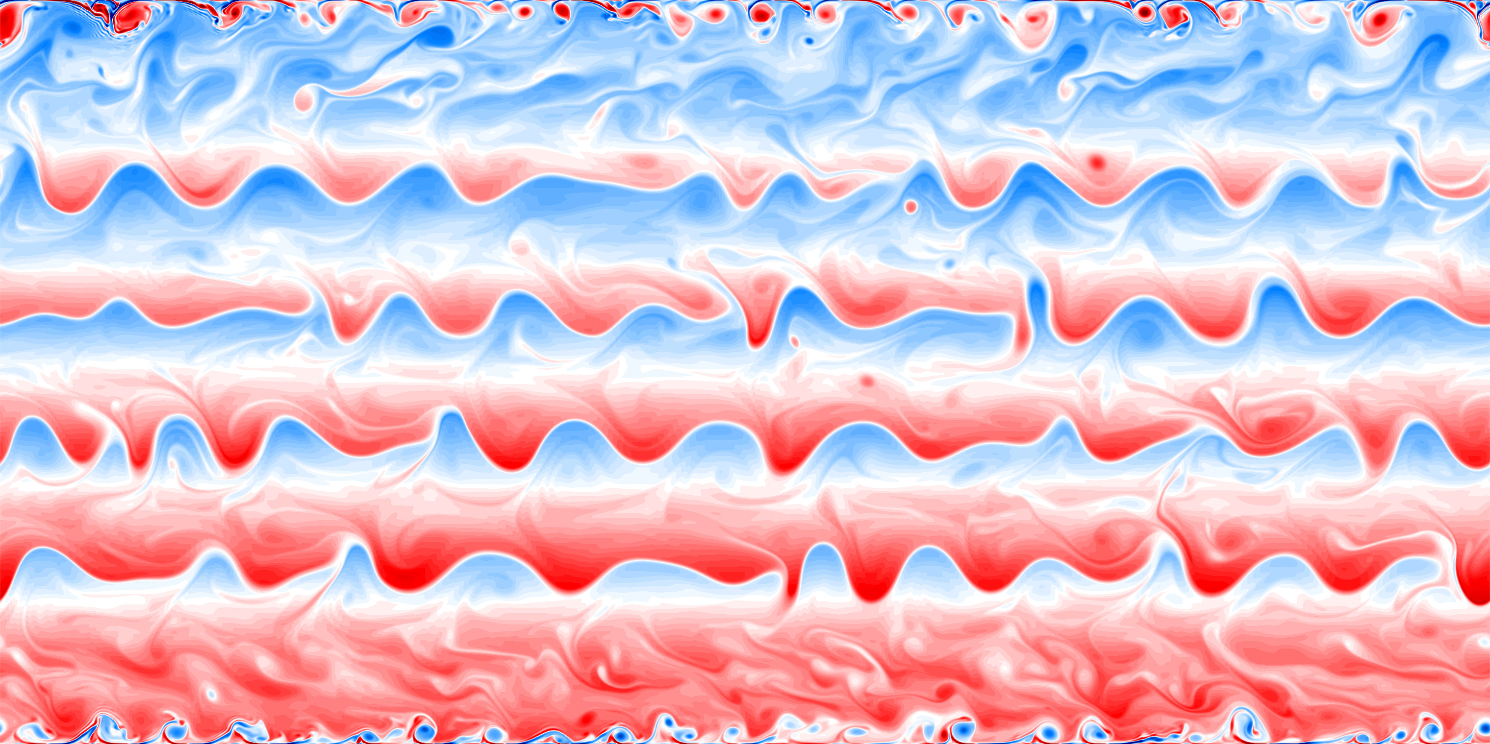
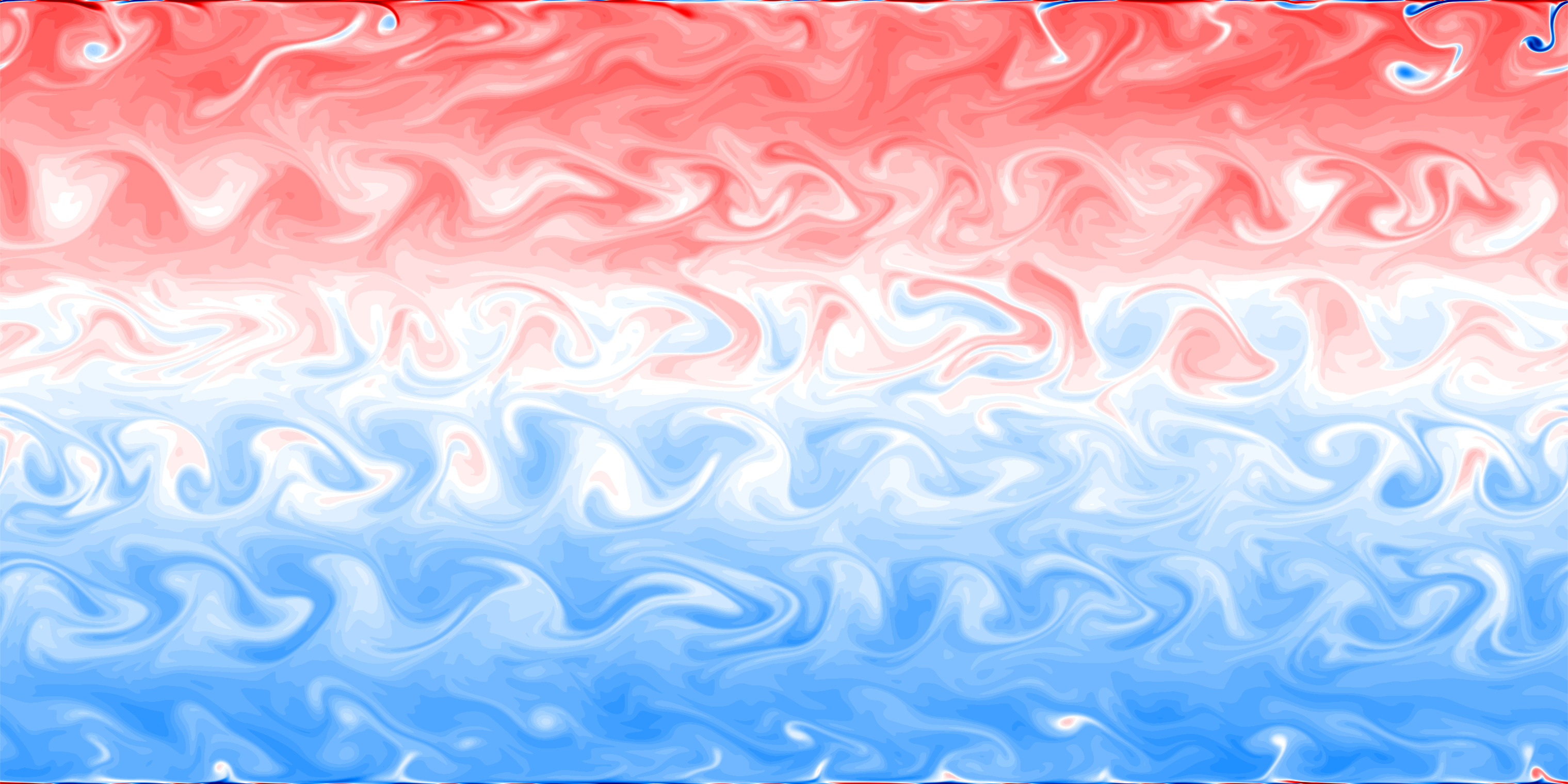
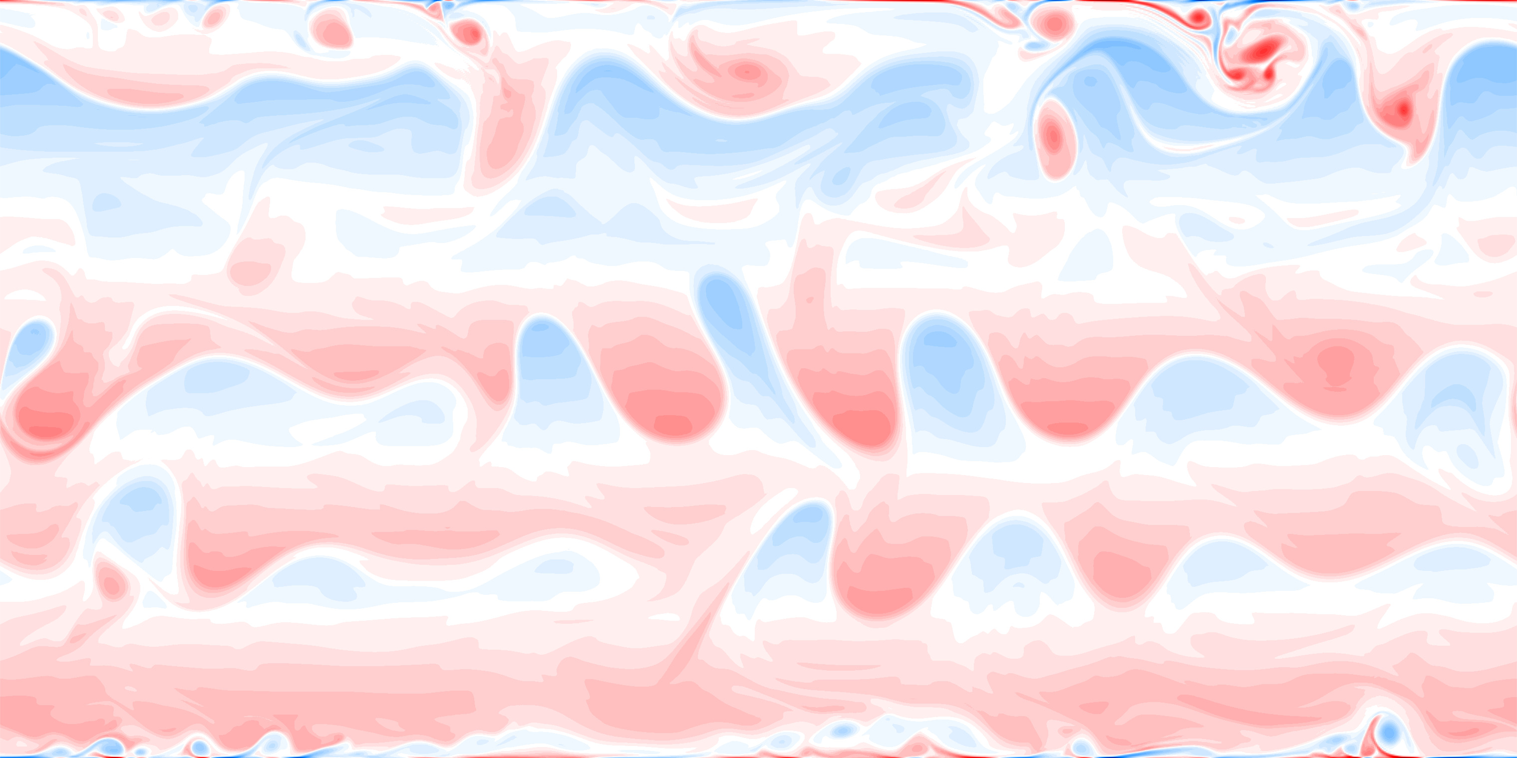
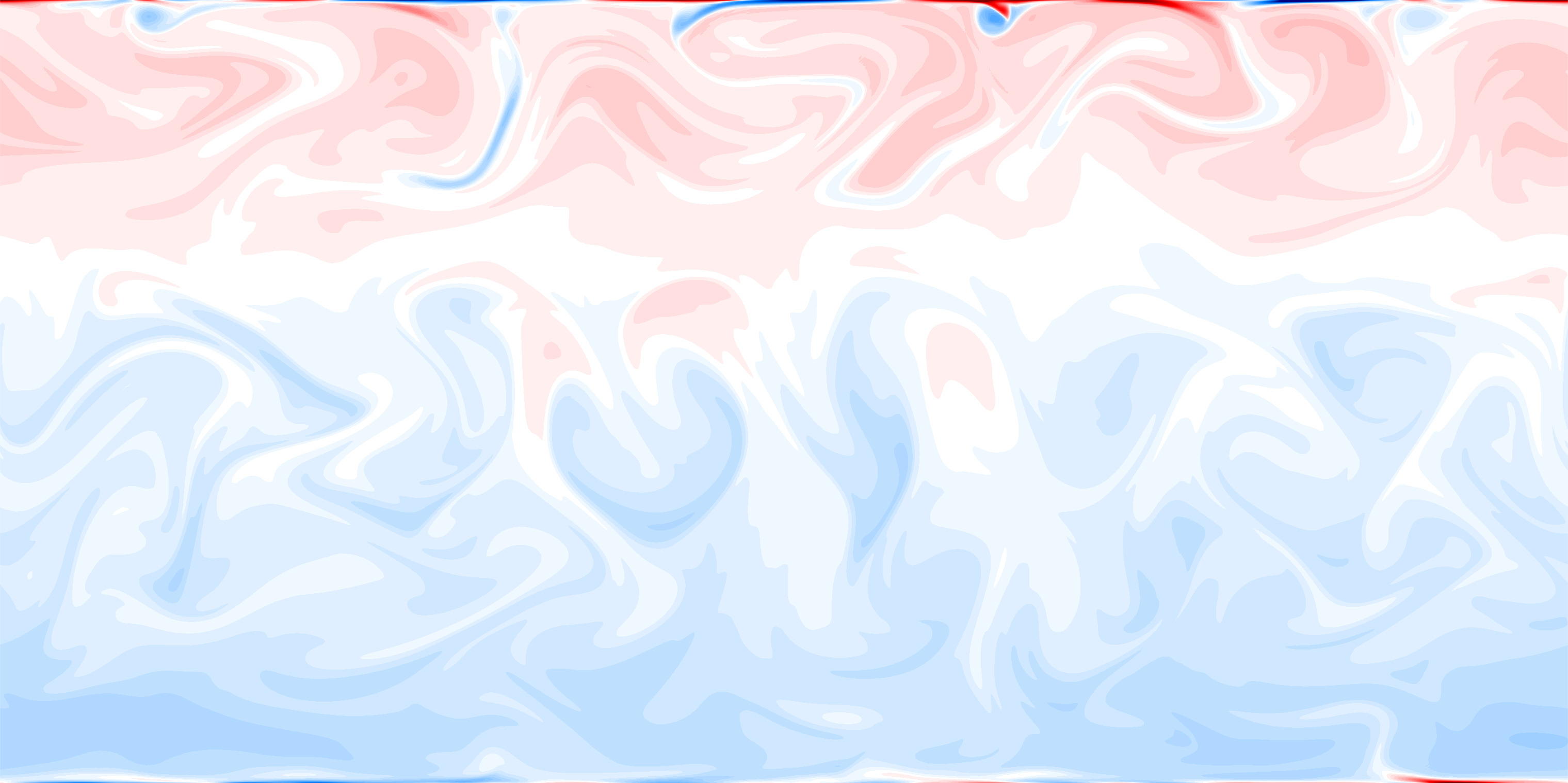
This paper complements the work done in CCHWS2019_3 where the ”true state” is chosen to be the solution of the Euler equation with forcing and damping. We choose the quasi-geostrophic (QG) equations for this work as it has a qualitatively different behaviour from Euler: As one can see in Fig. 1, the solution of the QG equations is far less homogeneous than the that of the Euler equation, exhibiting multiple large-scale zonally elongated jets as well as small-scale vortices. Indeed, one of the findings of our work is that the formation of jets is heavily influenced by the size of the grid: the coarser the grid the less jets are formed. Nevertheless, once data assimmilation is applied to the coarser model (stochastically parametrized and properly calibrated), the number of jets can be preserved. The occurrence of the jets makes the data assimilation problem harder. Whilst in CCHWS2019_3 it sufficed to use only tempering and jittering to assimilate the data, in the current work we obtained far better results only after we added the nudging procedure to the two already used in CCHWS2019_3 . Another difference from the work done in CCHWS2019_3 was the choice of the initial ensemble, which here chosen as a set of independent realizations from the solution of the stochastically perturbed QG equation. We found this to be a more natural alternative to the one used in CCHWS2019_3 .

The use of the combination of tempering and jittering is theoretically justified. Indeed in BCJ2016 it is shown that the use of the two procedures can produce particle filters suitable for solving high dimensional problems. More precisely, it is proved that the effective sample size of the ensemble of particles remains under control as the dimension $d$ of the underlying system increases with a computational cost that is at most quadratic in $d$. By contrast, a generic (bootstrap) particle filter would require a computational cost that is exponential in $d$.

As is usually the case in data assimilation, the particle filter proceeds by alternating between forecast and analysis cycles. In each analysis step, observations of the current (and possibly past) state of a system are combined with the results from a prediction model (the forecast) to produce an analysis. The tempering and jittering are used to complete the analysis step, whilst the nudging procedure is used in the forecast step. In the absence of nudging, the ensemble particles have trajectories that are independent solutions of the stochastic QG equations. Nudging consists in adding a drift to the trajectories of the particles with the aim of maximising the likelihood of their positions given the observation data. This introduces a bias in the system that is corrected at the analysis step. It follows that also the nudging procedure is theoretically justified through a standard convergence argument, see for example Crisan2002ASO . It follows that the data assimilation algorithm presented in this paper will give an asymptotically (as the number of particles increases) consistent approximation of the posterior distribution of the state given the data. That does not mean that the empirical distribution of the ensemble is a good approximation of the posterior. The size of the ensemble is 100 and this is certainly not enough to approximate a posterior distribution in a state space of dimension $O(10^{4})$. However, it offers a sound theoretical basis for the algorithms presented here. We give further details of this issue in Section 5.

The paper is structured as follows. In Section 2 we describe the deterministic N-layer QG equations and Hamiltonian formulation for the stochastic multi-layer QG model. Section 3 presents the deterministic and stochastic QG equations, and numerical methods for the QG model. In Section 4 we prove that the stochastic CABARET scheme is consistent with the stochastic QG equation in the mean square sense in time. In Section 5 we discuss different procedures used: Bootstrap Particle Filter, jittering, tempering and nudging procedures. In Section 6 we present and discuss the numerical experiments and results, and study how the data assimilation methods influence the quality of the forecast given by the stochastic QG model. The following is a summary of the main numerical experiments contained in this paper:

• Dependence of the relative bias and the ensemble mean $l_{2}$-norm relative error between the true deterministic solution and its stochastic parameterisation on the data assimilation step (Figs. 4 and 6), grid resolution (Fig. 8), data assimilation methods (Figs. 10 and 12), and the number of weather stations (Figs. 14 and 15);

• Analysis of how uncertainty of the stochastic spread is influenced by the data assimilation step (Figs. 5 and 7), grid resolution (Fig. 9), data assimilation methods (Figs. 11 and 13), and the number of weather stations (Figs. 16 and 17);

• Forecast reliability rank histrograms for the stochastic QG model with and without the data assimilation procedure (Fig. 18).

Finally, Section 7 concludes the present work and discusses the outlook for future research.

2 Hamiltonian equations of motion for a multi-layer fluid

2.1 The deterministic $N$-layer quasi-geostrophic (NLQG) equations

Consider a stratified fluid of $N$ superimposed layers of constant densities $\rho_{1}<\dots<\rho_{N}$; the layers being stacked according to increasing density, such that the density of the upper layer is $\rho_{1}$. The quasi-geostrophic (QG) approximation assumes that the velocity field is constant in the vertical direction and that in the horizontal direction the motion obeys a system of coupled incompressible shallow water equations. We shall denote by $\mathbf{u}_{i}=(-\,\partial_{y}\psi_{i},\partial_{x}\psi_{i})=\mathbf{\hat{z}}\times\nabla\psi_{i}$ the velocity field of the $i^{th}$ layer, where $\psi_{i}$ is its stream function, and the layers are numbered from the top to the bottom. We define the potential vorticity of the $i^{th}$ layer as

$$\omega_{i}=q_{i}+f_{i}=\Delta\psi_{i}+\alpha_{i}\sum\limits^{N}_{j=1}T_{ij}\psi_{j}+f_{i}=:\sum\limits^{N}_{j=1}E_{ij}\psi_{j}+f_{i}\,,\qquad i=1,\dots,N,$$ (1)

where the potential vorticity is defined as $\omega_{i}=q_{i}+f_{i}$, the elliptic operator $E_{ij}$ defines the layer vorticity,

$$q_{i}=\sum\limits^{N}_{j=1}E_{ij}\psi_{j}:=\Delta\psi_{i}+\alpha_{i}\sum\limits^{N}_{j=1}T_{ij}\psi_{j}\,,$$

and the constant parameters $\alpha_{i}$, $f_{i}$, $f_{0}$, $\beta$, $f_{N}$ are

$$\begin{split}\alpha_{i}&=(f_{0}^{2}/g)\big{(}(\rho_{i+1}-\rho_{i})/\rho_{0}\big{)}D_{i}\,,\qquad i=1,\dots,N,\\ f_{i}&=f_{0}+\beta y\,,\qquad i=1,\dots,N-1,\\ f_{N}&=f_{0}+\beta y+f_{0}d(y)/D_{N},\\ f_{0}&=2\Omega\sin(\phi_{0})\,,\qquad\beta=2\Omega\cos(\phi_{0})/R\,,\end{split}$$ (2)

where $g$ is the gravitational acceleration, $\rho_{0}=(1/N)(\rho_{1}+\dots+\rho_{N})$ is the mean density, $D_{i}$ is the mean thickness of the $i^{th}$ layer, $R$ is the Earth’s radius, $\Omega$ is the Earth’s angular velocity, $\phi_{0}$ is the reference latitude, and $d(y)$ is the shape of the bottom. The $N\times N$ symmetric tri-diagonal matrix $T_{ij}$ represents the second-order difference operator,

$$\sum\limits^{N}_{j=1}T_{ij}\psi_{j}=(\psi_{i-1}-\psi_{i})-(\psi_{i}-\psi_{i+1})\,,$$ (3)

so that

$$T_{ij}=\begin{bmatrix}-1&1&0&\ldots&\ldots&0\\ 1&-2&\ddots&\ddots&&\vdots\\ 0&\ddots&\ddots&\ddots&\ddots&\vdots\\ \vdots&\ddots&\ddots&\ddots&\ddots&0\\ \vdots&&\ddots&\ddots&-2&1\\ 0&\ldots&\ldots&0&1&-1\end{bmatrix}\,,\qquad i,j=1,\dots,N.$$ (4)

With these standard notations, the motion of the NLQG fluid is given by

$$\partial_{t}q_{i}=\Big{\{}\omega_{i},\,\psi_{i}\Big{\}}_{xy}=-\,\mathbf{\hat{z}}\times\nabla\psi_{i}\cdot\nabla\omega_{i}=-\,\mathbf{u}_{i}\cdot\nabla\omega_{i}\,,\qquad i=1,\dots,N,$$ (5)

where $\mathbf{\hat{z}}$ is the vertical unit vector, $\mathbf{u}_{i}=\mathbf{\hat{z}}\times\nabla\psi_{i}$ is the horizontal flow velocity in the $i^{th}$ layer, and the brackets in

$$\{\omega,\psi\}=J(\omega,\psi)=\omega_{x}\psi_{y}-\omega_{y}\psi_{x}=\mathbf{\hat{z}}\cdot\nabla\omega\times\nabla\psi$$ (6)

denote the usual $xy$ canonical Poisson bracket in $\mathbb{R}^{2}$. The boundary conditions in a compact domain $D\subset\mathbb{R}^{2}$ with smooth boundary $\cup_{j}\partial{D}_{j}$ are $\psi_{j}|_{(\partial{D}_{j})}=constant$, whereas in the entire $\mathbb{R}^{2}$ they are $\lim_{(x,y)\to\textpm\infty}\nabla\psi_{j}=0$. The space of variables with canonical Poisson bracket in (6) consists of $N$-tuples $(q_{1},\dots,q_{N})$ of real-valued functions on $D$ (the “generalized vorticities”) with the above boundary conditions and certain smoothness properties that guarantee that solutions are at least of class $C^{1}$. The Hamiltonian for the $N$-layer vorticity dynamics in (5) is the total energy

$$H(q_{1},\dots,q_{N})=\frac{1}{2}\int_{D}\Big{[}\sum\limits^{N}_{i=1}\frac{1}{\alpha_{i}}|\nabla\psi_{i}|^{2}+\sum\limits^{N-1}_{i=1}(\psi_{i+1}-\psi_{i})^{2}\Big{]}dx\,dy\,,\qquad i=1,\dots,N,$$ (7)

with stream function $\psi_{i}$ determined from vorticity $\omega_{i}$ by solving the elliptic equation (1) for $q_{i}=\omega_{i}-f_{i}$ with

$$q_{i}=\sum\limits^{N}_{j=1}E_{ij}\psi_{j}\,,$$ (8)

for the boundary conditions discussed above. Hence, we find that

$$H(q_{1},\dots,q_{N})=-\frac{1}{2}\int_{D}\sum\limits^{N}_{i,j=1}\psi_{i}E_{ij}\psi_{j}dx\,dy=-\frac{1}{2}\int_{D}\sum\limits^{N}_{i,j=1}q_{i}E^{-1}_{ij}*q_{j}dx\,dy=-\frac{1}{2}\int_{D}\sum\limits^{N}_{i=1}q_{i}\psi_{i}dx\,dy\,,$$ (9)

where $E^{-1}_{ij}*q_{j}=\psi_{i}$ denotes convolution with the Greens function $E^{-1}_{ij}$ for the symmetric elliptic operator $E_{ij}$. The relation (9) means that $\delta H/\delta q_{i}=\psi_{i}$ for the variational derivative of the Hamiltonian functional $H$ with respect to the function $q_{j}$.

Remark 1 (Lie–Poisson bracket)

Equations (5) are Hamiltonian with respect to the Lie–Poisson bracket on the dual of $\oplus\sum\limits^{N}_{i=1}{\cal F}(D)$ given by

$$\{F,H\}(q_{1},\dots,q_{N})=\sum\limits^{N}_{i=1}\int_{D}(q_{i}+f_{i}(x))\left\{\frac{\delta F}{\delta q_{i}},\,\frac{\delta H}{\delta q_{i}}\right\}_{xy}dx\,dy\,,$$ (10)

for arbitrary functions $F$ and $H$, provided the domain of flow $D$ is simply connected.

The motion equations (5) for $q_{i}$ now follow from the Lie–Poisson bracket (10) after an integration by parts to write it equivalently as

$$\frac{dF}{dt}=\{F,H\}(q_{1},\dots,q_{N})=-\sum\limits^{N}_{i=1}\int_{D}\frac{\delta F}{\delta q_{i}}\left\{q_{i}+f_{i}(x),\,\frac{\delta H}{\delta q_{i}}\right\}_{xy}dx\,dy\,,$$ (11)

and recalling that $\delta H/\delta q_{i}=-E^{-1}_{ij}*q_{j}=-\,\psi_{i}$, $i=1,2,\dots,N$, so that equations (5) follow.

Remark 2 (Constants of motion)

According to equations (5), the material time derivative of $\omega_{i}(t,x,y)$ vanishes along the flow lines of the divergence-free horizontal velocity $\mathbf{u}_{i}=\mathbf{\hat{z}}\times\nabla\psi_{i}$. Consequently, for every differentiable function $\Phi_{i}:\mathbb{R}\to\mathbb{R}$ the functional

$$C_{\Phi_{i}}(\omega_{i})=\int_{D}\Phi_{i}(\omega_{i})\,dx\,dy$$ (12)

is a conserved quantity for the system (5) for $i=1,\dots,N$, provided the integrals exist. By Kelvin’s circulation theorem, the following integrals over an advected domain $S(t)$ in the plane are also conserved,

$$I_{i}(t)=\int_{S(t)}\omega_{i}\,dx\,dy=\int_{\partial S(t)}\nabla\psi_{i}\cdot\mathbf{\hat{n}}\,ds\,,$$ (13)

where $\mathbf{\hat{n}}$ is the horizontal outward unit normal and $ds$ is the arclength parameter of the closed curve $\partial S(t)$ bounding the domain $S(t)$ moving with the flow.

2.2 Hamiltonian formulation for the stochastic NLQG fluid

Having understood the geometric structure (Lie–Poisson bracket, constants of motion and Kelvin circulation theorem) for the deterministic case, we can introduce the stochastic versions of equations (5) by simply making the Hamiltonian stochastic while preserving the previous geometric structure, as done in the previous section. Namely, we choose

$$h(t)=h(0)+\int_{0}^{t}H(\{q\})ds+\int_{0}^{t}\int_{D}\sum\limits^{N}_{i=1}\sum\limits^{K}_{k=1}q_{i}(s,x,y)\zeta^{k}_{i}(x,y)\,dx\,dy\circ dW_{k}(s)\,,$$ (14)

so that

$${\color[rgb]{1,0,0}\mathsf{d}}h=H(\{q\})dt+\int_{D}\sum\limits^{N}_{i=1}\sum\limits^{K}_{k=1}q_{i}(t,x,y)\zeta^{k}_{i}(x,y)\,dx\,dy\circ dW_{k}(t)\,,$$ (15)

where the $\zeta^{k}_{i}(x,y)$, $k=1,\dots,K$ represent the correlations of the Stratonovich noise we have introduced in (15).

For this stochastic Hamiltonian, the Lie–Poisson bracket (10) leads to the following stochastic process for the transport of the $N$-layer generalised vortices,

$${\color[rgb]{1,0,0}\mathsf{d}}q_{i}=\Big{\{}\omega_{i},\,{\color[rgb]{1,0,0}\mathsf{d}}\psi\Big{\}}_{xy}=J\big{(}\omega_{i},\,{\color[rgb]{1,0,0}\mathsf{d}}\psi\big{)}=\nabla({\color[rgb]{1,0,0}\mathsf{d}}\psi_{i})\times\mathbf{\hat{z}}\cdot\nabla\omega_{i}=-\,{\color[rgb]{1,0,0}\mathsf{d}}\mathbf{u}_{i}\cdot\nabla\omega_{i}\,,\qquad i=1,\dots,N,$$ (16)

where we have defined the stochastic transport velocity in the $i^{th}$ layer

$${\color[rgb]{1,0,0}\mathsf{d}}\mathbf{u}_{i}:=\mathbf{\hat{z}}\times\nabla({\color[rgb]{1,0,0}\mathsf{d}}\psi_{i})\,,\qquad i=1,\dots,N,$$ (17)

in terms of its stochastic stream function

$${\color[rgb]{1,0,0}\mathsf{d}}\psi_{i}:=\psi_{i}\,dt+\sum\limits^{K}_{k=1}\zeta^{k}_{i}(x,y)\circ dW_{k}(t)={\color[rgb]{1,0,0}\mathsf{d}}\frac{\delta h}{\delta q_{i}}\,,\qquad i=1,\dots,N,$$ (18)

determined from the variational derivative of the stochastic Hamiltonian in (15) with respect to the generalised vorticity $q_{i}$ in the $i^{th}$ layer.

Remark 3 (Constants of motion)

The constants of motion $C_{\Phi_{i}}$ in (12) and the Kelvin circulation theorem for the integrals $I_{i}$ in (13) persist for the stochastic generalised vorticity equations in (16). This is because both of these properties follow from the Lie-Poisson bracket in (10). However, the stochastic Hamiltonian in (15) is not conserved, since it depends explicitly on time, $t$, through its Stratonovich noise term.

3 The two-dimensional multilayer quasi-geostrophic model

3.1 Deterministic case

The two-layer deterministic QG equations for the potential vorticity (PV) anomaly $q$ in a domain $\Omega$ are given by the PV material conservation law augmented with forcing and dissipation Pedlosky1987 ; Vallis2006 :

$$\frac{\partial q_{1}}{\partial t}+\mathbf{u}_{1}\cdot\nabla q_{1} =\nu\Delta^{2}\psi_{1}-\beta\frac{\partial\psi_{1}}{\partial x},$$ (19)

$$\frac{\partial q_{2}}{\partial t}+\mathbf{u}_{2}\cdot\nabla q_{2} =\nu\Delta^{2}\psi_{2}-\mu\Delta\psi_{2}-\beta\frac{\partial\psi_{2}}{\partial x},$$

where $\psi$ is the stream function, $\beta$ is the planetary vorticity gradient, $\mu$ is the bottom friction parameter, $\nu$ is the lateral eddy viscosity, and $\mathbf{u}=(u,v)$ is the velocity vector. The computational domain $\Omega=[0,L_{x}]\times[0,L_{y}]\times[0,H]$ is a horizontally periodic flat-bottom channel of depth $H=H_{1}+H_{2}$ given by two stacked isopycnal fluid layers of depth $H_{1}$ and $H_{2}$. A mollified version of the existence and uniqueness theorem for the QG model can be found in Farhat_et_al2012 .

Forcing in (19) is introduced via a vertically sheared, baroclinically unstable background flow (e.g., BerloffKamenkovich2013 )

$$\psi_{i}\rightarrow-U_{i}\,y+\psi_{i},\quad i=1,2,$$ (20)

where the parameters $U_{i}$ are background-flow zonal velocities.

The PV anomaly and stream function are related through two elliptic equations:

$$q_{1}=\Delta\psi_{1}+s_{1}(\psi_{2}-\psi_{1}),$$ (21a)

$$q_{2}=\Delta\psi_{2}+s_{2}(\psi_{1}-\psi_{2}),$$ (21b)

with stratification parameters $s_{1}$, $s_{2}$.

System (19)-(21) is augmented by the integral mass conservation constraint McWilliams1977

$$\frac{\partial}{\partial t}\iint\limits_{\Omega}(\psi_{1}-\psi_{2})\ dydx=0,$$ (22)

by the periodic horizontal boundary conditions,

$$\boldsymbol{\psi}\Big{|}_{\Gamma_{2}}=\boldsymbol{\psi}\Big{|}_{\Gamma_{4}}\,,\quad\boldsymbol{\psi}=(\psi_{1},\psi_{2})\,,$$ (23)

and no-slip boundary conditions

$$\boldsymbol{u}\Big{|}_{\Gamma_{1}}=\boldsymbol{u}\Big{|}_{\Gamma_{3}}=0\,.$$ (24)

set at northern and southern boundaries of the domain.

3.1.1 Numerical method

The QG model (19)-(24) is solved with the CABARET method, which is based on a second-order, non-dissipative and low-dispersive, conservative advection scheme Karabasov_et_al2009 . The CABARET scheme can simulate large-Reynolds-number flow regimes at lower computational costs compared to conventional methods (see, e.g., Arakawa1966 ; WoodwardColella1984 ; ShuOsher1988 ; Hundsdorfer_et_al1995 ), since the scheme is low dispersive and non-oscillatory.

The CABARET method is a predictor-corrector scheme in which the components of the conservative variables are updated at half time steps. Algorithm 1 illustrates the principal steps of the CABARET method adopted from Karabasov_et_al2009 . To make the notation more concise, we introduce the forward difference operators in space

$$\Delta_{x}[f]=\frac{f_{i+1,j}-f_{ij}}{\Delta x},\quad\Delta_{y}[f]=\frac{f_{i,j+1}-f_{ij}}{\Delta y},$$

and omit spatial and layer indices wherever possible, unless stated otherwise. The time step of the CABARET scheme is denoted by $\tau$.

Algorithm 1 CABARET scheme for the deterministic QG system (19)-(24)

  Predictor

  $\displaystyle q^{n+\frac{1}{2}}_{i+\frac{1}{2},j+\frac{1}{2}}=q^{n}_{i+\frac{1}{2},j+\frac{1}{2}}+\frac{\Delta t}{2}\,F\left(q^{n},u(q^{n}),v(q^{n})\right)+\Delta t\,F_{\beta}\left(v^{n},v^{n-1}\right)+\Delta t\,F_{\rm visc}\left(\psi\left(q^{n+\frac{1}{2}}\right)\right)$,

   $F\left(q^{n}_{ij},u(q^{n}),v(q^{n})\right)=-\left(\Delta_{x}\left[(uq)^{n}_{i,j+\frac{1}{2}}\right]+\Delta_{y}\left[(vq)^{n}_{i+\frac{1}{2},j}\right]\right)$,

   $\displaystyle F_{\beta}\left(v^{n},v^{n-1}\right)=\frac{3}{2}R^{n}-\frac{1}{2}R^{n-1},\quad R^{n}=-\frac{\beta}{2}\left(v^{n}_{i+\frac{1}{2},j+1}+v^{n}_{i+\frac{1}{2},j}\right)$.

   The forcing term

$$F_{\rm visc}\left(\psi\left(q^{n+\frac{1}{2}}\right)\right)=\nu\left(\Delta^{2}\psi_{l}\right)^{n+\frac{1}{2}}_{i+\frac{1}{2},j+\frac{1}{2}}-\delta_{2l}\,\mu\left(\Delta\psi_{l}\right)^{n+\frac{1}{2}}_{i+\frac{1}{2},j+\frac{1}{2}},\,l=1,2$$

 is added in the prediction step after the elliptic problem is solved.

   Solve the elliptic system of equations with respect to $(\psi_{1})^{n+\frac{1}{2}}_{i+\frac{1}{2},j+\frac{1}{2}}$ and $(\psi_{2})^{n+\frac{1}{2}}_{i+\frac{1}{2},j+\frac{1}{2}}$

    $\displaystyle(q_{1})^{n+\frac{1}{2}}_{i+\frac{1}{2},j+\frac{1}{2}}=\left(\Delta\psi_{1}\right)^{n+\frac{1}{2}}_{i+\frac{1}{2},j+\frac{1}{2}}+s_{1}\left(\psi_{[21]}\right)^{n+\frac{1}{2}}_{i+\frac{1}{2},j+\frac{1}{2}},\quad(q_{2})^{n+\frac{1}{2}}_{i+\frac{1}{2},j+\frac{1}{2}}=\left(\Delta\psi_{2}\right)^{n+\frac{1}{2}}_{i+\frac{1}{2},j+\frac{1}{2}}+s_{2}\left(\psi_{[12]}\right)^{n+\frac{1}{2}}_{i+\frac{1}{2},j+\frac{1}{2}}\,.$

   Calculate

    $\displaystyle\psi^{n+\frac{1}{2}}_{ij}=\frac{1}{4}\left(\psi^{n+\frac{1}{2}}_{i+\frac{1}{2},j+\frac{1}{2}}+\psi^{n+\frac{1}{2}}_{i+\frac{1}{2},j-\frac{1}{2}}+\psi^{n+\frac{1}{2}}_{i-\frac{1}{2},j+\frac{1}{2}}+\psi^{n+\frac{1}{2}}_{i-\frac{1}{2},j-\frac{1}{2}}\right).$

   Update velocity components at the cell faces

    $\displaystyle u^{n+\frac{1}{2}}_{i,j+\frac{1}{2}}=\Delta_{y}\left[\psi^{n+\frac{1}{2}}_{ij}\right],\quad\left(v_{l}\right)^{n+\frac{1}{2}}_{i+\frac{1}{2},j}=-\Delta_{x}\left[\psi^{n+\frac{1}{2}}_{ij}\right].$

  Extrapolator

   $\displaystyle u^{n+1}_{i,j+\frac{1}{2}}=\frac{3}{2}u^{n+\frac{1}{2}}_{i,j+\frac{1}{2}}-\frac{1}{2}u^{n-\frac{1}{2}}_{i,j+\frac{1}{2}}\,,\quad v^{n+1}_{i,j+\frac{1}{2}}=\frac{3}{2}v^{n+\frac{1}{2}}_{i,j+\frac{1}{2}}-\frac{1}{2}v^{n-\frac{1}{2}}_{i,j+\frac{1}{2}}$.

   $\displaystyle q^{n+1}_{i+1,j+\frac{1}{2}}=2q^{n+\frac{1}{2}}_{i+\frac{1}{2},j+\frac{1}{2}}-q^{n}_{i,j+\frac{1}{2}}$ if $\displaystyle u^{n+1}_{i+1,j+\frac{1}{2}}\geq 0$;  $\displaystyle q^{n+1}_{i,j+\frac{1}{2}}=2q^{n+\frac{1}{2}}_{i+\frac{1}{2},j+\frac{1}{2}}-q^{n}_{i+1,j+\frac{1}{2}}$ if $\displaystyle u^{n+1}_{i,j+\frac{1}{2}}<0$.

   $\displaystyle q^{n+1}_{i+\frac{1}{2},j+1}=2q^{n+\frac{1}{2}}_{i+\frac{1}{2},j+\frac{1}{2}}-q^{n}_{i+\frac{1}{2},j}$ if $\displaystyle v^{n+1}_{i+\frac{1}{2},j+1}\geq 0$;  $\displaystyle q^{n+1}_{i+\frac{1}{2},j}=2q^{n+\frac{1}{2}}_{i+\frac{1}{2},j+\frac{1}{2}}-q^{n}_{i+\frac{1}{2},j+1}$ if $\displaystyle v^{n+1}_{i+\frac{1}{2},j}<0$.

   Correction of the computed cell-face PV anomaly values

    If $q^{n+1}_{i,j+\frac{1}{2}}>M^{n+1}_{i,j+\frac{1}{2}}\Rightarrow q^{n+1}_{i,j+\frac{1}{2}}=M^{n+1}_{i,j+\frac{1}{2}}$; If $q^{n+1}_{i,j+\frac{1}{2}}<m^{n+1}_{i,j+\frac{1}{2}}\Rightarrow q^{n+1}_{i,j+\frac{1}{2}}=m^{n+1}_{i,j+\frac{1}{2}}$.

    If $q^{n+1}_{i+\frac{1}{2},j}>M^{n+1}_{i+\frac{1}{2},j}\Rightarrow q^{n+1}_{i+\frac{1}{2},j}=M^{n+1}_{i+\frac{1}{2},j}$; If $q^{n+1}_{i+\frac{1}{2},j}<m^{n+1}_{i+\frac{1}{2},j}\Rightarrow q^{n+1}_{i+\frac{1}{2},j}=m^{n+1}_{i+\frac{1}{2},j}$.

    $\text{If}\,\,u^{n+1}_{i+1,j+\frac{1}{2}}\geq 0\quad\left\{\begin{array}[]{ll}M^{n+1}_{i+1,j+\frac{1}{2}}=\max\left(q^{n}_{i,j+\frac{1}{2}},q^{n}_{i+\frac{1}{2},j+\frac{1}{2}},q^{n}_{i+1,j+\frac{1}{2}}\right)+\tau Q^{n}_{i+\frac{1}{2},j+\frac{1}{2}},\\ m^{n+1}_{i+1,j+\frac{1}{2}}=\min\left(q^{n}_{i,j+\frac{1}{2}},q^{n}_{i+\frac{1}{2},j+\frac{1}{2}},q^{n}_{i+1,j+\frac{1}{2}}\right)+\tau Q^{n}_{i+\frac{1}{2},j+\frac{1}{2}}.\\ \end{array}\right.$

  

    $\text{If}\,\,u^{n+1}_{i,j+\frac{1}{2}}<0\quad\left\{\begin{array}[]{ll}M^{n+1}_{i,j+\frac{1}{2}}=\max\left(q^{n}_{i,j+\frac{1}{2}},q^{n}_{i+\frac{1}{2},j+\frac{1}{2}},q^{n}_{i+1,j+\frac{1}{2}}\right)+\tau Q^{n}_{i+\frac{1}{2},j+\frac{1}{2}},\\ m^{n+1}_{i,j+\frac{1}{2}}=\min\left(q^{n}_{i,j+\frac{1}{2}},q^{n}_{i+\frac{1}{2},j+\frac{1}{2}},q^{n}_{i+1,j+\frac{1}{2}}\right)+\tau Q^{n}_{i+\frac{1}{2},j+\frac{1}{2}}.\\ \end{array}\right.$

    $\displaystyle Q^{n+\frac{1}{2}}_{i+\frac{1}{2},j+\frac{1}{2}}=\frac{q^{n+\frac{1}{2}}_{i+\frac{1}{2},j+\frac{1}{2}}-q^{n}_{i+\frac{1}{2},j+\frac{1}{2}}}{\Delta t/2}+\frac{1}{2}\left((u_{l})^{n+1}_{i+1,j+\frac{1}{2}}+(u_{l})^{n+1}_{i,j+\frac{1}{2}}\right)\Delta_{x}\left[q^{n}_{i,j+\frac{1}{2}}\right]$.

  Corrector

  $\displaystyle q^{n+1}_{i+\frac{1}{2},j+\frac{1}{2}}=q^{n+\frac{1}{2}}_{i+\frac{1}{2},j+\frac{1}{2}}+\frac{\Delta t}{2}\,F\left(q^{n+1},u(q^{n+1}),v(q^{n+1})\right)$, where $q^{n+1}$, $u(q^{n+1})$, $v(q^{n+1})$ are computed in the extrapolation step.

3.2 Stochastic case

The stochastic version of the QG equations (19) is given by holm2015variational :

$$\begin{split}{\color[rgb]{1,0,0}\mathsf{d}}q_{1}+\left(\mathbf{u}_{1}\,dt+{\color[rgb]{1,0,0}\sum\limits^{K}_{k=1}\xi^{k}_{1}\circ dW^{k}_{t}}\right)\cdot\nabla q_{1}&=\left(\nu\Delta^{2}\psi_{1}-\beta\frac{\partial\psi_{1}}{\partial x}\right)\,dt,\\ {\color[rgb]{1,0,0}\mathsf{d}}q_{2}+\left(\mathbf{u}_{2}\,dt+{\color[rgb]{1,0,0}\sum\limits^{K}_{k=1}\xi^{k}_{2}\circ dW^{k}_{t}}\right)\cdot\nabla q_{2}&=\left(\nu\Delta^{2}\psi_{2}-\mu\Delta\psi_{2}-\beta\frac{\partial\psi_{2}}{\partial x}\right)\,dt.\end{split}$$ (25)

The stochastic terms marked in red color is the only difference from the deterministic QG model (19), all other equations remain the same as in the deterministic case. However, the CABARET scheme in the stochastic case differs from the deterministic version and therefore its use can only be justified if it is consistent with the stochastic QG model. In other words, the CABARET scheme should be in the Stratonovich form.

3.2.1 Numerical method

The CABARET scheme for the stochastic QG system (25) is given by Algorithm 2 (with the stochastic terms highlighted in red). To the best of our knowledge, the CABARET scheme has not been applied to the stochastic QG equations, and is used in this work for the first time.

Algorithm 2 The CABARET scheme for the stochastic QG system

  Predictor

  

$$\begin{split}q^{n+\frac{1}{2}}_{i+\frac{1}{2},j+\frac{1}{2}}=q^{n}_{i+\frac{1}{2},j+\frac{1}{2}}&+\frac{\Delta t}{2}\,F\left(q^{n},u(q^{n}),v(q^{n})\right)+\Delta t\,F_{\beta}\left(v^{n},v^{n-1}\right)+\Delta t\,F_{\rm visc}\left(\psi\left(q^{n+\frac{1}{2}}\right)\right)\\ &+{\color[rgb]{1,0,0}\sum\limits^{K}_{k=1}\left(G_{k}\left(q^{n}\right)+G_{k,\beta}\right)\frac{\Delta W_{k}}{2}},\end{split}$$ (26)

   ${\color[rgb]{1,0,0}G_{k}(q^{n})=-\left(\Delta_{x}\left[(\xi^{u}_{k}q^{n})_{i,j+\frac{1}{2}}\right]+\Delta_{y}\left[(\xi^{v}_{k}q^{n})_{i+\frac{1}{2},j}\right]\right)}$,  $\displaystyle{\color[rgb]{1,0,0}G_{k,\beta}=3R^{n}-R^{n-1}},\,{\color[rgb]{1,0,0}R^{n}=-\frac{\beta}{2}\left((\xi^{u}_{k})_{i+\frac{1}{2},j+1}+(\xi^{v}_{k})_{i+\frac{1}{2},j}\right)}$.

   The forcing term

$$F_{\rm visc}\left(\psi\left(q^{n+\frac{1}{2}}\right)\right)=\nu\left(\Delta^{2}\psi_{l}\right)^{n+\frac{1}{2}}_{i+\frac{1}{2},j+\frac{1}{2}}-\delta_{2l}\,\mu\left(\Delta\psi_{l}\right)^{n+\frac{1}{2}}_{i+\frac{1}{2},j+\frac{1}{2}},\,l=1,2$$

 is added in the prediction step after the elliptic problem is solved.

   Solve the elliptic system of equations with respect to $(\psi_{1})^{n+\frac{1}{2}}_{i+\frac{1}{2},j+\frac{1}{2}}$ and $(\psi_{2})^{n+\frac{1}{2}}_{i+\frac{1}{2},j+\frac{1}{2}}$

    $\displaystyle(q_{1})^{n+\frac{1}{2}}_{i+\frac{1}{2},j+\frac{1}{2}}=\left(\Delta\psi_{1}\right)^{n+\frac{1}{2}}_{i+\frac{1}{2},j+\frac{1}{2}}+s_{1}\left(\psi_{[21]}\right)^{n+\frac{1}{2}}_{i+\frac{1}{2},j+\frac{1}{2}},\quad(q_{2})^{n+\frac{1}{2}}_{i+\frac{1}{2},j+\frac{1}{2}}=\left(\Delta\psi_{2}\right)^{n+\frac{1}{2}}_{i+\frac{1}{2},j+\frac{1}{2}}+s_{2}\left(\psi_{[12]}\right)^{n+\frac{1}{2}}_{i+\frac{1}{2},j+\frac{1}{2}}\,.$

   Calculate

    $\displaystyle\psi^{n+\frac{1}{2}}_{ij}=\frac{1}{4}\left(\psi^{n+\frac{1}{2}}_{i+\frac{1}{2},j+\frac{1}{2}}+\psi^{n+\frac{1}{2}}_{i+\frac{1}{2},j-\frac{1}{2}}+\psi^{n+\frac{1}{2}}_{i-\frac{1}{2},j+\frac{1}{2}}+\psi^{n+\frac{1}{2}}_{i-\frac{1}{2},j-\frac{1}{2}}\right).$

   Update velocity components at the cell faces

    $\displaystyle u^{n+\frac{1}{2}}_{i,j+\frac{1}{2}}=\Delta_{y}\left[\psi^{n+\frac{1}{2}}_{ij}\right],\quad\left(v_{l}\right)^{n+\frac{1}{2}}_{i+\frac{1}{2},j}=-\Delta_{x}\left[\psi^{n+\frac{1}{2}}_{ij}\right].$

  Extrapolator

   $\displaystyle u^{n+1}_{i,j+\frac{1}{2}}=\frac{3}{2}u^{n+\frac{1}{2}}_{i,j+\frac{1}{2}}-\frac{1}{2}u^{n-\frac{1}{2}}_{i,j+\frac{1}{2}}\,,\quad v^{n+1}_{i,j+\frac{1}{2}}=\frac{3}{2}v^{n+\frac{1}{2}}_{i,j+\frac{1}{2}}-\frac{1}{2}v^{n-\frac{1}{2}}_{i,j+\frac{1}{2}}$.

   $\displaystyle q^{n+1}_{i+1,j+\frac{1}{2}}=2q^{n+\frac{1}{2}}_{i+\frac{1}{2},j+\frac{1}{2}}-q^{n}_{i,j+\frac{1}{2}}$ if $\displaystyle u^{n+1}_{i+1,j+\frac{1}{2}}+{\color[rgb]{1,0,0}\Xi^{u}_{i+1,j+\frac{1}{2}}}\geq 0$;  $\displaystyle q^{n+1}_{i,j+\frac{1}{2}}=2q^{n+\frac{1}{2}}_{i+\frac{1}{2},j+\frac{1}{2}}-q^{n}_{i+1,j+\frac{1}{2}}$ if $\displaystyle u^{n+1}_{i,j+\frac{1}{2}}+{\color[rgb]{1,0,0}\Xi^{u}_{i,j+\frac{1}{2}}}<0$.

   $\displaystyle q^{n+1}_{i+\frac{1}{2},j+1}=2q^{n+\frac{1}{2}}_{i+\frac{1}{2},j+\frac{1}{2}}-q^{n}_{i+\frac{1}{2},j}$ if $\displaystyle v^{n+1}_{i+\frac{1}{2},j+1}+{\color[rgb]{1,0,0}\Xi^{v}_{i+\frac{1}{2},j+1}}\geq 0$;  $\displaystyle q^{n+1}_{i+\frac{1}{2},j}=2q^{n+\frac{1}{2}}_{i+\frac{1}{2},j+\frac{1}{2}}-q^{n}_{i+\frac{1}{2},j+1}$ if $\displaystyle v^{n+1}_{i+\frac{1}{2},j}+{\color[rgb]{1,0,0}\Xi^{v}_{i+\frac{1}{2},j}}<0$.

   ${\color[rgb]{1,0,0}\Xi^{u}_{ij}=\sum\limits^{K}_{k=1}\left(\xi^{u}_{k}\right)_{ij}\Delta W_{k}},\quad{\color[rgb]{1,0,0}\Xi^{v}_{ij}=\sum\limits^{K}_{k=1}\left(\xi^{v}_{k}\right)_{ij}\Delta W_{k}}$.

   Correction of the computed cell-face PV anomaly values

    If $q^{n+1}_{i,j+\frac{1}{2}}>M^{n+1}_{i,j+\frac{1}{2}}\Rightarrow q^{n+1}_{i,j+\frac{1}{2}}=M^{n+1}_{i,j+\frac{1}{2}}$; If $q^{n+1}_{i,j+\frac{1}{2}}<m^{n+1}_{i,j+\frac{1}{2}}\Rightarrow q^{n+1}_{i,j+\frac{1}{2}}=m^{n+1}_{i,j+\frac{1}{2}}$.

    If $q^{n+1}_{i+\frac{1}{2},j}>M^{n+1}_{i+\frac{1}{2},j}\Rightarrow q^{n+1}_{i+\frac{1}{2},j}=M^{n+1}_{i+\frac{1}{2},j}$; If $q^{n+1}_{i+\frac{1}{2},j}<m^{n+1}_{i+\frac{1}{2},j}\Rightarrow q^{n+1}_{i+\frac{1}{2},j}=m^{n+1}_{i+\frac{1}{2},j}$.

    $\text{If}\,\,u^{n+1}_{i+1,j+\frac{1}{2}}+{\color[rgb]{1,0,0}\Xi^{u}_{i+1,j+\frac{1}{2}}}\geq 0\quad\left\{\begin{array}[]{ll}M^{n+1}_{i+1,j+\frac{1}{2}}=\max\left(q^{n}_{i,j+\frac{1}{2}},q^{n}_{i+\frac{1}{2},j+\frac{1}{2}},q^{n}_{i+1,j+\frac{1}{2}}\right)+\tau Q^{n}_{i+\frac{1}{2},j+\frac{1}{2}},\\ m^{n+1}_{i+1,j+\frac{1}{2}}=\min\left(q^{n}_{i,j+\frac{1}{2}},q^{n}_{i+\frac{1}{2},j+\frac{1}{2}},q^{n}_{i+1,j+\frac{1}{2}}\right)+\tau Q^{n}_{i+\frac{1}{2},j+\frac{1}{2}}.\\ \end{array}\right.$

  

    $\text{If}\,\,u^{n+1}_{i,j+\frac{1}{2}}+{\color[rgb]{1,0,0}\Xi^{u}_{i,j+\frac{1}{2}}}<0\quad\left\{\begin{array}[]{ll}M^{n+1}_{i,j+\frac{1}{2}}=\max\left(q^{n}_{i,j+\frac{1}{2}},q^{n}_{i+\frac{1}{2},j+\frac{1}{2}},q^{n}_{i+1,j+\frac{1}{2}}\right)+\tau Q^{n}_{i+\frac{1}{2},j+\frac{1}{2}},\\ m^{n+1}_{i,j+\frac{1}{2}}=\min\left(q^{n}_{i,j+\frac{1}{2}},q^{n}_{i+\frac{1}{2},j+\frac{1}{2}},q^{n}_{i+1,j+\frac{1}{2}}\right)+\tau Q^{n}_{i+\frac{1}{2},j+\frac{1}{2}}.\\ \end{array}\right.$

    $\displaystyle Q^{n+\frac{1}{2}}_{i+\frac{1}{2},j+\frac{1}{2}}=\frac{q^{n+\frac{1}{2}}_{i+\frac{1}{2},j+\frac{1}{2}}-q^{n}_{i+\frac{1}{2},j+\frac{1}{2}}}{\Delta t/2}+\frac{1}{2}\left(\left(u^{n+1}_{i+1,j+\frac{1}{2}}+{\color[rgb]{1,0,0}\Xi^{u}_{i+1,j+\frac{1}{2}}}\right)+\left(u^{n+1}_{i,j+\frac{1}{2}}+{\color[rgb]{1,0,0}\Xi^{u}_{i,j+\frac{1}{2}}}\right)\right)\Delta_{x}\left[q^{n}_{i,j+\frac{1}{2}}\right]$.

  Corrector

  

$$q^{n+1}_{i+\frac{1}{2},j+\frac{1}{2}}=q^{n+\frac{1}{2}}_{i+\frac{1}{2},j+\frac{1}{2}}+\frac{\Delta t}{2}\,F\left(q^{n+1},u(q^{n+1}),v(q^{n+1})\right)+{\color[rgb]{1,0,0}\sum\limits^{K}_{k=1}\left(G_{k}\left(q^{n+1}\right)+G_{k,\beta}\right)\frac{\Delta W_{k}}{2}}\,,$$ (27)

where $q^{n+1}$, $u(q^{n+1})$, $v(q^{n+1})$ are computed in the extrapolation step.

In order to show that the CABARET scheme is consistent with the stochastic QG model, we rewrite the scheme as the improved Euler method (also known as Heun’s method) KloedenPlaten1999 ,

$$\begin{split}x^{*}=&x^{n}+\Delta tf(x^{n})+{\color[rgb]{1,0,0}\Delta Wg(x^{n})},\\ x^{n+1}=&x^{n}+\frac{\Delta t}{2}(f(x^{n})+f(x^{*}))+{\color[rgb]{1,0,0}\frac{\Delta W}{2}(g(x^{n})+g(x^{*}))},\end{split}$$

which solves stochastic differential equations (SDEs) in the form of Stratonovich.

In doing so, we omit the space indices for the potential vorticity anomaly $q$ to emphasize the functional dependence on $q$, and introduce an extra variable

$$q^{*}=2q^{n+\frac{1}{2}}-q^{n},$$

which allows to recast (26) and (27) (see Algorithm 2) in the form

$$q^{*}=q^{n}+\Delta t\,F\left(q^{n},u(q^{n}),v(q^{n})\right)+2\Delta t\,F_{\beta}\left(v^{n},v^{n-1}\right)+2\Delta t\,F_{\rm visc}\left(\psi\left(q^{n+\frac{1}{2}}\right)\right)\\ +{\color[rgb]{1,0,0}\sum\limits^{K}_{k=1}\left(G_{k}(q^{n})+G_{k,\beta}\right){\Delta W_{k}}},\\$$ (28a)

$$q^{n+1}=\frac{q^{*}+q^{n}}{2}+\frac{\Delta t}{2}\,F\left(q^{*},u(q^{*}),v(q^{*})\right)+{\color[rgb]{1,0,0}\sum\limits^{K}_{k=1}\left(G_{k}\left(q^{*}\right)+G_{k,\beta}\right)\frac{\Delta W_{k}}{2}}.$$ (28b)

Substitution of (28a) into (28b) and (26) into the forcing term $F_{\rm visc}\left(\psi\left(q^{n+\frac{1}{2}}\right)\right)$ leads to

$$\begin{split}q^{n+1}=q^{n}&+\frac{\Delta t}{2}\,\left[F(q^{n},u(q^{n}),v(q^{n}))+F(q^{n}+{\color[rgb]{1,0,0}O_{1}(\Delta W_{k})},u(q^{n}+{\color[rgb]{1,0,0}O_{1}(\Delta W_{k})}),v(q^{n}+{\color[rgb]{1,0,0}O_{1}(\Delta W_{k})}))\right]\\ &+\Delta t\,\left[F_{\beta}\left(v^{n},v^{n-1}\right)+F_{\rm visc}\left(\psi\left(q^{n}+{\color[rgb]{1,0,0}O_{2}(\Delta W_{k})}\right)\right)\right]\\ &+{\color[rgb]{1,0,0}\sum\limits^{K}_{k=1}\left(G_{k}\left(q^{n}\right)+G_{k,\beta}\right)\frac{\Delta W_{k}}{2}}+{\color[rgb]{1,0,0}\sum\limits^{K}_{k=1}\left(G_{k}\left(q^{n}+O_{1}(\Delta W_{k})\right)+G_{k,\beta}\right)\frac{\Delta W_{k}}{2}},\end{split}$$ (29)

where

$$\begin{split}O_{1}(\Delta W_{k}):=&\Delta t\,F\left(q^{n},u(q^{n}),v(q^{n})\right)+2\Delta t\,F_{\beta}\left(v^{n},v^{n-1}\right)\\ +&2\Delta t\,F_{\rm visc}\left(\psi\left(q^{n}+{\color[rgb]{1,0,0}O_{2}(\Delta W_{k})}\right)\right){\color[rgb]{1,0,0}+\sum\limits^{K}_{k=1}\left(G_{k}\left(q^{n}\right)+G_{k,\beta}\right)\Delta W_{k}}\,,\end{split}$$

and

$$O_{2}(\Delta W_{k}):=\frac{\Delta t}{2}\,F\left(q^{n},u(q^{n}),v(q^{n})\right)+\Delta t\,F_{\beta}\left(v^{n},v^{n-1}\right)+{\color[rgb]{1,0,0}\sum\limits^{K}_{k=1}\left(G_{k}\left(q^{n}\right)+G_{k,\beta}\right)\frac{\Delta W_{k}}{2}}\,.$$

Retaining the terms up to order $\Delta t$ in (29) we get

$$\begin{split}q^{n+1}=q^{n}&+\Delta t\,\left[F(q^{n},u(q^{n}),v(q^{n}))+F_{\beta}\left(v^{n},v^{n-1}\right)+F_{\rm visc}\left(\psi(q^{n})\right)\right]\\ &+{\color[rgb]{1,0,0}\sum\limits^{K}_{k=1}\left(G_{k}\left(q^{n}\right)+G_{k,\beta}\right)\Delta W_{k}+{\color[rgb]{1,0,0}\sum\limits^{K}_{k_{1}=1}\sum\limits^{K}_{k_{2}=1}G_{k_{1}}\left(G_{k_{2}}(q^{n})+G_{k_{2},\beta}\right)\frac{\Delta W_{k_{1}}\Delta W_{k_{2}}}{2}}}+H.O.T.\,,\\ \end{split}$$ (30)

where $G_{\beta}$ does not depend on $q^{n}$, and $H.O.T.$ denotes higher order terms. Thus we have shown that the CABARET scheme is in Stratonovich form up to order $(\Delta t)^{3/2}$.

4 Consistency in time of the stochastic CABARET scheme

In this section we prove that the stochastic CABARET scheme (30) is consistent with the stochastic QG equation (25) in the mean square sense in time, since its consistency in space is guaranteed by its second order approximation Karabasov_et_al2009 . We consider a Stratonovich process $q=q(t,\mathbf{x})$, $\mathbf{x}=(x,y)$ satisfying the SPDE

$${\color[rgb]{1,0,0}\mathsf{d}}q=a_{t}\operatorname{d}t+{\color[rgb]{1,0,0}\sum\limits^{K}_{i=1}b_{i,t}\circ\operatorname{d}W_{i,t}},\quad a_{t}:=F(q^{n},u(q^{n}),v(q^{n}))+F_{\beta}+F_{\rm visc}\left(\psi(q^{n})\right),\quad b_{i,t}:=G_{i}(q^{n})+G_{i,\beta},$$

and rewrite it in the Itô form

$${\color[rgb]{1,0,0}\mathsf{d}}q=a_{t}\operatorname{d}t+{\color[rgb]{1,0,0}\sum\limits^{K}_{i=1}b_{i,t}\operatorname{d}W_{i,t}}+\frac{1}{2}\sum\limits^{K}_{i=1}b_{i,t}(b_{i,t})\operatorname{d}t\,,$$

or alternatively

$${\color[rgb]{1,0,0}\mathsf{d}}q=q_{d}\operatorname{d}t+{\color[rgb]{1,0,0}\sum\limits^{K}_{i=1}q^{i}_{s,t}\operatorname{d}W_{i,t}}$$ (31)

with the stochastic and deterministic parts defined as $\displaystyle q_{d}:=a_{t}+\frac{1}{2}\sum\limits^{K}_{i=1}b_{i,t}(b_{i,t})$ and $\displaystyle q^{i}_{s,t}:=b_{i,t}$, respectively.

We define consistency for SPDE (31) as follows

Definition 1

We say that a discrete time-space approximation $q^{n}=q^{n}_{d}+q^{n}_{s}$ of $q=q_{d}+q_{s}$ with the time step $\Delta t$ and space steps $\Delta\mathbf{x}=(\Delta x_{1},\Delta x_{2},\ldots,\Delta x_{d})$ is consistent in mean square of order $\alpha>1$ and $\beta>1$ in time and space with respect to (31) if there exists a nonnegative function $c=c((\Delta t)^{\alpha},(\Delta\mathbf{x})^{\beta})$ with $\lim\limits_{\begin{subarray}{c}\Delta t\rightarrow 0\\ \Delta\mathbf{x}\rightarrow 0\end{subarray}}c((\Delta t)^{\alpha},(\Delta\mathbf{x})^{\beta})=0$ such that

$$\mathbb{E}\left[\left\|q_{s}-q^{n}_{s}\right\|^{2}_{L^{2}(\Omega)}\right]\leq c((\Delta t)^{\alpha},(\Delta\mathbf{x})^{\beta})\,,\qquad\mathbb{E}\left[\left\|q_{d}-q^{n}_{d}\right\|^{2}_{L^{2}(\Omega)}\right]\leq c((\Delta t)^{\alpha},(\Delta\mathbf{x})^{\beta})$$

for all fixed values $q^{n}$, time $n=0,1,2,\ldots$ and space indices.

Since our focus in this section is on consistency in time, we have to prove that the following estimation holds:

$$\mathbb{E}\left[\left\|q_{s}-q^{n}_{s}\right\|^{2}_{L^{2}(\Omega)}\right]\leq c((\Delta t)^{\alpha})\,.$$ (32)

Theorem 4.1

Assuming that there exists a constant $\widetilde{C}>0$ such that the following assumptions hold

1. $\mathbb{E}\left[\left\|a_{r}-a_{s}\right\|_{L^{2}(\Omega)}\right]\leq\widetilde{C}\sqrt{r-s}$,

2. $\mathbb{E}\left[\left\|\sum\limits^{K}_{i=1}(b_{i,r}-b_{i,s})\right\|_{L^{2}(\Omega)}\right]\leq\widetilde{C}\sqrt{r-s}$,

3. $\mathbb{E}\left[\left\|\sum\limits^{K}_{i=1}\sum\limits^{K}_{j=1}b_{i,s}(b_{j,s})\right\|_{L^{2}(\Omega)}\right]\leq\widetilde{C}$, for $i,j=1,2,\ldots,m$,

4. $\mathbb{E}\left[\left\|\sum\limits^{K}_{i=1}(b_{i,r}(b_{i,r})-b_{i,s}(b_{i,s}))\right\|_{L^{2}(\Omega)}\right]\leq\widetilde{C}\sqrt{r-s}$,

5. $\mathbb{E}\left[\left\|{H.O.T.}\right\|\right]\leq\widetilde{C}(r-s)^{3/2}$,

with $\left|r-s\right|\leq\Delta t$, the stochastic CABARET scheme (30) is consistent in mean square with $c(\Delta t)=(\Delta t)^{2}$.

Proof

Integration of (31) with respect to time over the interval $[s,t]$ gives

$$q_{t}=q_{s}+\int\limits^{t}_{s}a_{r}\,dr+{\color[rgb]{1,0,0}\int\limits^{t}_{s}\sum\limits^{K}_{i=1}b_{i,r}\,dW_{i,r}}+\frac{1}{2}\int\limits^{t}_{s}\sum\limits^{K}_{i=1}b_{i,r}(b_{i,r})dr\,.$$ (33)

Substitution of (30) and (33) into (32) leads to

$$\begin{split}&\mathbb{E}\left[\left\|\int\limits^{t}_{s}a_{r}\,dr+{\color[rgb]{1,0,0}\int\limits^{t}_{s}\sum\limits^{K}_{i=1}b_{i,r}\,dW_{i,r}}+\frac{1}{2}\int\limits^{t}_{s}\sum\limits^{K}_{i=1}b_{i,r}(b_{i,r})dr\right.\right.\\ &-\left.\left.\left(a_{t}\Delta t+{\color[rgb]{1,0,0}\sum\limits^{K}_{i=1}b_{i,s}\,\Delta W_{i,s}}+{\color[rgb]{1,0,0}\frac{1}{2}\sum\limits^{K}_{i,j=1}b_{i,s}(b_{j,s})\Delta W_{i,s}\Delta W_{j,s}}\right)+{H.O.T.}\right\|^{2}_{L^{2}(\Omega)}\right]\leq c(\Delta t).\end{split}$$ (34)

By combining the terms in (34), we get

$$\mathbb{E}\left[\left\|A+B+C\right\|^{2}_{L^{2}(\Omega)}\right]\leq c(\Delta t),$$ (35)

where

$$A:=\int\limits^{t}_{s}(a_{r}-a_{s}),dr\quad B:={\color[rgb]{1,0,0}\int\limits^{t}_{s}\sum\limits^{K}_{i=1}(b_{i,r}-b_{i,s})\,dW_{i,r}},\quad C:=C_{1}-C_{2}-C_{3},$$

with

$$C_{1}:=\frac{1}{2}\int\limits^{t}_{s}\sum\limits^{K}_{i=1}(b_{i,r}(b_{i,r})-b_{i,s}(b_{i,s}))\,dr,\quad C_{2}:=\frac{1}{2}\sum\limits^{K}_{i=1}b_{i,s}(b_{i,s})({\color[rgb]{1,0,0}(\Delta W_{i})^{2}}-\Delta t),\quad C_{3}:={\color[rgb]{1,0,0}\frac{1}{2}\sum\limits^{K}_{i\neq j}b_{i,s}(b_{j,s})\Delta W_{i}\Delta W_{j}}\,.$$

Applying the triangle and Young’s inequalities to (35) we arrive at

$$\mathbb{E}\left[\left\|A+B+C\right\|^{2}_{L^{2}(\Omega)}\right]\leq 3\mathbb{E}\left[\left\|A\right\|^{2}_{L^{2}(\Omega)}+\left\|B\right\|^{2}_{L^{2}(\Omega)}+\left\|C\right\|^{2}_{L^{2}(\Omega)}+\widetilde{C}^{2}(\Delta t)^{3}\right].$$

Using A2, the Cauchy–Schwarz inequality and A1, we estimate the first term as

$$\mathbb{E}\left[\left\|A\right\|^{2}_{L^{2}(\Omega)}\right]\leq\Delta t\,\mathbb{E}\left[\int\limits^{t}_{s}\left\|a_{r}-a_{s}\right\|^{2}_{L^{2}(\Omega)}\,dr\right]\leq\frac{\widetilde{C}^{2}}{2}(\Delta t)^{3}.$$

Estimation of the second term is given by

$$\mathbb{E}\left[\left\|B\right\|^{2}_{L^{2}(\Omega)}\right]= \int\limits_{\Omega}\mathbb{E}\left[{\color[rgb]{1,0,0}\left(\int\limits^{t}_{s}\sum\limits^{K}_{i=1}(b_{i,r}-b_{i,s})\,dW_{i,r}\right)^{2}}\right]\,d\Omega$$ (using the Itô isometry)

$$= \mathbb{E}\left[\int\limits_{\Omega}\int\limits^{t}_{s}\left(\sum\limits^{K}_{i=1}(b_{i,r}-b_{i,s})\right)^{2}\,dr\,d\Omega\right]$$ (the Cauchy–Schwarz inequality leads to)

$$\leq \Delta t\,\mathbb{E}\left[\int\limits^{t}_{s}\left\|\sum\limits^{K}_{i=1}(b_{i,r}-b_{i,s})\right\|^{2}_{L^{2}(\Omega)}\,dr\right]\leq\frac{\widetilde{C}^{2}}{2}(\Delta t)^{3}$$ (using A2).

To estimate the term $C$ in (35), we use the triangle inequality to get

$$\mathbb{E}\left[\left\|C\right\|^{2}_{L^{2}(\Omega)}\right]\leq\mathbb{E}\left[\left\|C_{1}\right\|^{2}_{L^{2}(\Omega)}+\left\|C_{2}\right\|^{2}_{L^{2}(\Omega)}+\left\|C_{3}\right\|^{2}_{L^{2}(\Omega)}\right]\,,$$

and then separately estimate each term on the right hand side.

Applying the Cauchy–Schwarz inequality and A4 to $C_{1}$, we get the following estimation

$$\mathbb{E}\left[\left\|C_{1}\right\|^{2}_{L^{2}(\Omega)}\right]\leq\frac{\Delta t}{2}\mathbb{E}\left[\int\limits_{\Omega}\left\|\sum\limits^{K}_{i=1}(b_{i,r}(b_{i,r})-b_{i,s}(b_{i,s}))\right\|^{2}_{L^{2}(\Omega)}\,d\Omega\right]\leq\frac{\widetilde{C}^{2}}{8}(\Delta t)^{3}.$$

The term $C_{2}$ is estimated as

$$\mathbb{E}\left[\left\|C_{2}\right\|^{2}_{L^{2}(\Omega)}\right]= \int\limits_{\Omega}\mathbb{E}\left[\left(\frac{1}{2}\sum\limits^{K}_{i=1}(b_{i,s}(b_{i,s}))\left({\color[rgb]{1,0,0}(\Delta W_{i})^{2}}-\Delta t\right)\right)^{2}\right]\,d\Omega$$

$$= \frac{1}{4}\int\limits_{\Omega}\sum\limits^{K}_{i=1}(b_{i,s}(b_{i,s}))^{2}\,\mathbb{E}\left[{\color[rgb]{1,0,0}(\Delta W_{i})^{4}}-2{\color[rgb]{1,0,0}(\Delta W_{i})^{2}}\Delta t+(\Delta t)^{2}\right]\,d\Omega$$

$$= \frac{(\Delta t)^{2}}{2}\left\|\sum\limits^{K}_{i=1}(b_{i,s}(b_{i,s}))^{2}\right\|^{2}_{L^{2}(\Omega)}\leq\frac{\widetilde{C}^{2}}{2}(\Delta t)^{2}$$ (using A3).

Using A3 for $C_{3}$ leads to

$$\mathbb{E}\left[\left\|C_{3}\right\|^{2}_{L^{2}(\Omega)}\right]=\frac{1}{4}\int\limits_{\Omega}\sum\limits^{K}_{i\neq j}(b_{i,s}(b_{i,s}))^{2}\,\mathbb{E}\left[{\color[rgb]{1,0,0}(\Delta W_{i})^{2}}\right]\mathbb{E}\left[{\color[rgb]{1,0,0}(\Delta W_{j})^{2}}\right]\,d\Omega=\frac{(\Delta t)^{2}}{4}\left\|\sum\limits^{K}_{i\neq j}(b_{i,s}(b_{i,s}))\right\|^{2}_{L^{2}(\Omega)}\leq\frac{\widetilde{C}^{2}}{4}(\Delta t)^{2}.$$

Finally, we arrive at the following estimation

$$\mathbb{E}\left[\left\|A+B+C\right\|^{2}_{L^{2}(\Omega)}\right]\leq C^{*}\left((\Delta t)^{2}+(\Delta t)^{3}\right)\leq C^{*}(\Delta t)^{2},\quad C^{*}>0,$$

which proves the theorem.

Remark 4

Conditions A1-A5 are satisfied and SPDE (31) is well-posed for sufficiently large p for all $T>0$ if the stochastic QG equation (25) has a solution in $W^{2p,2}$ such that $\mathbb{E}\left[\sup\limits_{t\in[0,T]}||q_{i}||^{2}_{W^{2p,2}}\right]<\infty$, $i=1,2$.

5 Data assimilation methods

We find it useful to describe the framework and the data assimilation methodology through the language of nonlinear filtering. For this purpose, let us consider a probability space $(\Omega,\mathcal{F},\mathbb{P})$ on which we define a pair of processes $Z$ and $Y$. The process $Z$ is normally called the signal process, and the process $Y$ models the observational data and is called the observation process. In the context of this work the signal process, also called the true state, is given by the solution of the deterministic QG equation (19) computed on a fine grid $G_{f}=2049\times 1025$ and projected onto a coarse grid, denoted by $G_{s}$ (details below), by spatially averaging the high-resolution stream function $\psi^{f}$ over the corresponding coarse grid cells.

The filtering problem consists in computing/approximating the posterior distribution of the signal $Z_{t}$, denoted by $\pi_{t}$ given the observations $Y_{s}$, $s\in[0,t]$. In our context, the observations consist of noisy measurements of the true state recorded at discrete times (every 2 or 4 hours) and are taken at locations (called weather stations) on a data grid $G_{d}$ defined below. The data assimilation is performed at these times, which we call the assimilation times.

The most basic particle filter, called the bootstrap particle filter (see section 5.1 for details) uses ensembles of, say, $N$ particles that evolve according to the law of the signal between assimilation times. At the data assimilation times, each particle is weighed according to the likelihood of its position given the new data. A new set of particles is then obtained by sampling $N$ times (with replacement) from the set of weighted particles. The end result is that particles with high likelihoods (close to the true trajectory) are kept and possibly multiplied, and particles with small likelihoods (that are away from the true trajectory) are eliminated. As a result, the ensemble of particles should stay closer to the true trajectory when compared to the particles that evolve according to the signal distribution. The bootstrap particle filter described below uses multiple copies of the signal which, in our case, would require the resolution of the deterministic QG equation (19) on a fine grid $G_{f}=2049\times 1025$. Each run of the particle filter at such a high resolution is very expensive computationally (one data assimilation step takes approximately 15 minutes). Taking into account that we assimilate data over thousands steps, the computational resources needed are too large. For this reason we replace the true state with a proxy. We use a process $X$ defined on the same probability space whose sample paths are a lot cheaper to simulate. In our case, the process $X$ will be the solution of the stochastic QG equation (25) computed on the (signal) grid $G_{s}$ (each run of the process $X$ requires around 20 seconds). This replacement is a form of model reduction: we reduce the dimension of the underlying state from $G_{f}=2049\times 1025$ to $G_{s}=129\times 65$. This model reduction is critical to successful implementation of the data assimilation procedure. It is also rigorously justified as we explain now.

The posterior distribution $\pi_{t}$ depends continuously on two constituents: the (prior) distribution of the signal and the observation data. That means that if we replace the original signal distribution with a proxy distribution, we will still obtain a good approximation of $\pi_{t}$ provided the original and the proxy distributions are close to each other in some suitably chosen topology on the space of distribution.

For the current work, the way in which we ensure that two distributions (original and proxy) remains close to each other is by adding the right type of stochasticity to the model and “in the right directions”. This is done through the Stochastic Advection by Lie Transport (SALT) approach holm2015variational . The stochasticity is calibrated to match the fluctuations of $X$ as explained in see CCHWS2019_1 ; CCHWS2019_2 . We emphasize that one does not seek a pathwise approximation of the true state, but only an approximation of its distribution.

In our case, the true state is deterministic, and the process $X$ is random. As we saw in CCHWS2019_1 ; CCHWS2019_2 , one can visualise the distribution of $X$ through ensembles of particles with trajectories that are solutions of the stochastic QG equation (25) computed on the grid $G_{s}$ and driven by independent families of Brownian motions. In the language of uncertainty quantification, the difference between the two distributions is interpreted as the “uncertainty of the model”. Typically, the ensemble of particles is a spread ”around” the true trajectory, the size of the spread measuring the (model) uncertainty. To visualise this one can look at projections of the true trajectory and the ensembles of particles at various grid points. Of course, the more refined the grid $G_{s}$ is, the closer the two distributions are, and the smaller the spread. However, refining the grid $G_{s}$ leads to an increase in the computational effort of generating the particle trajectories. One of the roles of data assimilation is to reduce the spread (the uncertainty) without refining the grid.

The average position of the ensemble of particles obtained through the data assimilation, denoted by $\widehat{Z}_{t}$, is a pointwise estimate of the true state $Z_{t}$, whilst the spread of the ensemble is a measure of the approximation error $Z_{t}-\widehat{Z}_{t}$. As explained in the introduction, the data assimilation methodology presented here is asymptotically consistent: the empirical distribution of the particles converges, as $N\mapsto\infty$ to the posterior distribution $\pi_{t}$ Crisan2002ASO . As a consequence, $\widehat{Z}_{t}$ converges to the conditional expectation of the true state $Z_{t}$ given the observations, and the empirical covariance matrix converges to the conditional expectation of $(Z_{t}-\widehat{Z}_{t})(Z_{t}-\widehat{Z}_{t})^{T}$ given the observations.. This is true if the particles evolve according to the original distribution of the signal. In our case we use a proxy distribution, so the limit will be an approximation of $\pi_{t}$, the difference between this approximation and $\pi_{t}$ being controlled by the choice of the signal grid $G_{s}$.

The data assimilation methodology described below consists in combination between the bootstrap particle filter and three additional procedures: nudging, tempering and jittering. The bootstrap particle filter cannot be used on its own to solve the data assimilation problem. The reason is that the particle likelihoods vary wildly from each other. That is because the particle themselves stray away from the true state rapidly and in different directions. This is reflected through observation data. One particle likelihood or a small number of such likelihoods will become much higher than the rest, and only the corresponding particle(s) will be selected and multiplied. This will not offer a good representation of the posterior distribution. As we will explain below the additional procedures will eliminate this effect ensuring a reasonably spread set of particles.

In the next subsections we study how each of these individual procedures influences the accuracy of the estimation $\widehat{Z}_{t}$ and the quality of the forecast given by the stochastic QG model. In order to study how the dimension of the observation process $Y$ (the number of weather stations) affects data assimilation, we consider two different data grids $G_{d}=\{4\times 4,8\times 4\}$. We also study stochastic solutions on two different signal grids $G_{s}=\{129\times 65,257\times 129\}$ in order to highlight the effect of more accurate proxy distributions on the results.

As stated above, we will use ensembles $\mathcal{S}$ of solutions of the stochastic QG equation (25) driven by independent realizations of the Brownian noise $W$. For the purpose of this paper, the size of the ensemble is taken to be $N=100$ and the number of Brownian motion (independent sources of stochasticity) is taken to be $K=32$; as already stated, the elements of the ensembles will be called particles. It was numerically shown in CCHWS2019_2 that $N=100$ and $K=32$ is enough to reasonably approximate the fluctuations of the original distribution. Through numerical experiments, we showed that the spread of the ensemble will not increase substantially by taking more particles and/or sources of noise (Brownian motions).

The observations data $Y_{t}$ is, in our case, an $M$-dimensional process that consists of noisy measurements of the velocity field $\mathbf{u}$ taken at a point belonging to the data grid $G_{d}$:

$$Y_{t}:={\rm P}^{s}_{d}(Z_{t})+\eta,$$

where $\mathcal{P}^{s}_{d}:G_{s}\rightarrow G_{d}$ is a projection operator from the signal grid $G_{s}$ to the data grid $G_{d}$, $\eta=\mathcal{N}(\mathbf{0},I_{\sigma})$ is a normally distributed random vector, with mean vector $\mathbf{0}=(0,\ldots,0)$ and diagonal covariance matrix $I_{\sigma}=diag(\sigma_{1}^{2},\ldots,\sigma_{M}^{2})$. Rather than choosing an arbitrary $\sigma=(\sigma_{1},\ldots,\sigma_{M})$ for the standard deviation of the noise, we use the standard deviation of the velocity field computed over the coarse grid cell of the signal grid.

We introduce the likelihood-weight function

$$\mathcal{W}(\mathbf{X},\mathbf{Y})=\exp\left(-\frac{1}{2}\sum\limits^{M}_{i=1}\left\|\frac{{\rm P}^{s}_{d}(X_{i})-Y_{i}}{\sigma_{i}}\right\|^{2}_{2}\right),$$ (36)

with $M$ being the number of grid points (weather stations). In order to measure the variability of the weights (36) of particles we use the effective sample size:

$${\rm ESS}(\overline{\mathbf{w}})=\left(\sum\limits^{N}_{i=1}\left(\overline{w}_{i}\right)^{2}\right)^{-1},\quad\overline{\mathbf{w}}:=\mathbf{w}\left(\sum\limits^{N}_{i=1}w_{i}\right)^{-1},$$ (37)

which is close to the ensemble size $N$ if the particles have weights that are close to each other, and decays to one, as the ensemble degenerates (i.e. there are fewer and fewer particles with large weights and the rest have small weights). One should resample for the weighted ensemble if the ESS drops below a given threshold, $N^{*}$,

$${\rm ESS}<N^{*}.$$

We chose $N^{*}=80$ to be our threshhold.

5.1 Bootstrap particle filter

In this section we consider the most basic particle filter, called the bootstrap particle filter or Sampling Importance Resampling filter DFG2001 . This method works as follows.

Given an initial distribution of particles, each particle is propagated forward according to the stochastic QG equation. Then, based on partial observations, $\mathbf{Y}_{t_{j+1}}$ of the true state, the weights of new particles are computed, and if the effective sample size drops below the critical value $N^{*}$, the particles are resampled to remove particles with small weights.

Algorithm 3 Bootstrap particle filter

  for $j=0,1,2,\ldots$ do

     Solve  ${\color[rgb]{1,0,0}\mathsf{d}}q^{(n)}_{i}+\left(\mathbf{u}^{(n)}_{i}\,dt+{\color[rgb]{1,0,0}\sum\limits^{K}_{k=1}\xi^{k}_{i}\circ dW^{(n)}_{k}}\right)\cdot\nabla q^{(n)}_{i}=F^{(n)}_{i}\,dt,\quad i=1,2;\quad t\in[t_{j},t_{j+1}],\quad n\in[1..N].$

     Obtain observation $\mathbf{Y}_{t_{j+1}}$ from weather stations

     Compute $\overline{\mathbf{w}}:=\mathcal{W}(\mathbf{q}_{t_{j+1}},\mathbf{Y}_{t_{j+1}})$

     if ${\rm ESS(\overline{\mathbf{w}})}<N^{*}$ then

        $\mathbf{q}_{t_{j+1}}:={\bf Resample}(\overline{\mathbf{w}})$

     end if

  end for

For a high dimensional problem such as the one studied in this paper, the effective sample size drops very quickly to 1 as the sample degenerates rapidly. The reason for this is that particles travel very quickly away from the true state, and this is picked up by the observation data (unless the measurement noise is large which is not in our case - the observations are accurate). To counteract this, the resampling procedure would need to be performed unreasonably frequently or a large number of particles would need to be used.

To maintain the diversity of the ensemble we use instead three additional procedures: the tempering technique and jittering based on the Metropolis-Hastings Markov chain Monte Carlo (MCMC) method. We explain each of these procedures in the following sub-sections.

5.2 Tempering and Jittering

We will explain briefly the usage of these two procedures, see CCHWS2019_3 for further details. The idea behind tempering is to artificially flatten the weights thorough rescaling the log likelihoods by a factor $\phi\in(0,1]$, which is called temperature. Once this is done resampling can be applied. This gives a much more diverse ensemble as the ESS will have more reasonable values (the temperature is specifically chosen to ensure this). However, some of resulting particles will still have duplicates. To eliminate these, one uses jittering.

Jittering is another technique which improves the diversity of the ensemble by computing new particles which have been duplicated during resampling. There are different ways how to diversify the ensemble. For example, one can jitter the particles by simply adding some random perturbations to them. However, in this case, the perturbed particles are not the solutions of the stochastic QG equation that, in turn, can lead to nonphysical behaviour of the model. Instead, we compute new particles by solving the stochastic QG equation driven by the Brownian motion $\rho W+\sqrt{1-\rho^{2}}\,d\widetilde{W}$, where $W$ is the original Brownian motion $W$ and $\widetilde{W}$ is a new Brownian motion independent of $W$. The perturbation parameter $\rho$ is chosen so that particles are not placed too far from the original position, yet far enough to ensure the diversity of the sample. In our experiments, we use $\rho=0.9999$. Each new proposal for the position of the particle is then accepted/rejected thorough a standard Metropolis-Hastings method, in which $M_{1}$ stands for the number of iterations; we choose $M_{1}=20$. This ensures that the perturbations do not change the sought distribution.

Of course, after the first tempering-jittering cycle has finished, the particles in the resulting ensemble are samples of the altered distribution which is not what we desire, therefore the procedure is repeated by finding the next temperature value in the range $(\varphi,1]$ that offers a reasonable ESS. This is repeated until the temperature scaling is 1 so that the original distribution is recovered. The tempering-jittering methodology is given by Algorithm 4 below.

Algorithm 4 Particle Filter with Tempering and MCMC

  for $j=0,1,2,\ldots$ do

     Solve  ${\color[rgb]{1,0,0}\mathsf{d}}q^{(n)}_{i}+\left(\mathbf{u}^{(n)}_{i}\,dt+{\color[rgb]{1,0,0}\sum\limits^{K}_{k=1}\xi^{k}_{i}\circ dW^{(n)}_{k}}\right)\cdot\nabla q^{(n)}_{i}=F^{(n)}_{i}\,dt,\quad i=1,2;\quad t\in[t_{j},t_{j+1}],\quad n\in[1..N].$

     Obtain observation $\mathbf{Y}_{t_{j+1}}$ from weather stations

     Compute $\overline{\mathbf{w}}:=\mathcal{W}(\mathbf{q}_{t_{j+1}},\mathbf{Y}_{t_{j+1}})$

     if ${\rm ESS(\overline{\mathbf{w}})}<N^{*}$ then

        Find $p$ such that $ESS(\overline{\mathbf{w}})\geq N^{*}$, where $\overline{\mathbf{w}}:=\mathcal{W}^{1/p}(\mathbf{q}_{t_{j+1}},\mathbf{Y}_{t_{j+1}})$

        for $k=1,2,\ldots,p$ do

           Compute $\overline{\mathbf{w}}:=\mathcal{W}^{\phi_{k}}(\mathbf{q}_{t_{j+1}},\mathbf{Y}_{t_{j+1}}),\ \phi_{k}:=\frac{k}{p}$

           $\mathbf{q}_{t_{j+1}}:={\bf Resample}(\overline{\mathbf{w}})$

           for $m=1,2,\ldots,M_{1}$ do

              ${\color[rgb]{1,0,0}\Xi^{(n)}_{i}:=\sum\limits^{K}_{k=1}\xi_{k,i}\circ\left(\rho\,dW^{(n)}_{k}+\sqrt{1-\rho^{2}}\,d\widetilde{W}^{(n)}_{k}\right)},\quad n\in[1..N]$

              Solve  ${\color[rgb]{1,0,0}\mathsf{d}}\widetilde{q}^{(n)}_{i}+\left(\widetilde{\mathbf{u}}^{(n)}_{i}\,dt+{\color[rgb]{1,0,0}\Xi^{(n)}_{i}}\right)\cdot\nabla\widetilde{q}^{(n)}_{i}=\widetilde{F}^{(n)}_{i}\,dt,\quad i=1,2;\quad t\in[t_{j},t_{j+1}],\quad n\in[1..N]$

              for n=1,2,…,N do

                 $\alpha:=\left(\mathcal{W}(\widetilde{q}^{(n)}_{t_{j+1}},Y^{(n)}_{t_{j+1}})/\mathcal{W}(q^{(n)}_{t_{j+1}},Y^{(n)}_{t_{j+1}})\right)^{\phi_{k}}$

                 if $1\leq\alpha$ then

                    $q^{(n)}_{t_{j+1}}:=\widetilde{q}^{(n)}_{t_{j+1}}$

                 else if $\mathcal{U}[0,1]<\alpha$ then

                    $q^{(n)}_{t_{j+1}}:=\widetilde{q}^{(n)}_{t_{j+1}}$

                 end if

              end for

           end for

        end for

     end if

  end for

5.3 Nudging

Tempering combined with jittering is a powerful technique which can correctly narrow the stochastic spread in the presence of informative data, while also maintaining the diversity of the ensemble over a long time period. Their combined success depends crucially on the quality of the original sample proposals. This quality is produced by evolving the particles using the SPDE (the proxy distribution) and not the true distribution. To reduce the discrepancy introduced in this way, one can use nudging. The idea of nudging is to correct the solution of SPDE (25) so as to keep the particles closer to the true state. To do so, we add a ‘nudging term’ (marked in blue) to SPDE (25),

$${\color[rgb]{1,0,0}\mathsf{d}}q_{i}(\lambda)+\left(\mathbf{u}_{i}(\lambda)\,dt+{\color[rgb]{1,0,0}\sum\limits^{K}_{k=1}\xi^{k}_{i}\circ dW^{k}_{t}}+{\color[rgb]{0,0,1}\sum\limits_{k=1}^{K}\boldsymbol{\xi}^{k}_{i}\lambda_{k}\,dt}\right)\cdot\nabla q_{i}(\lambda) =F_{i}\,dt,\quad i=1,2.$$ (38)

Note that $q$ depends on the parameter $\lambda$. The trajectories of the particles will be solutions of this perturbed SPDE (38). To account for the perturbation, the particles will have new weights according to Girsanov’s theorem, given by

$$\mathcal{W}({\mathbf{q}}(\lambda),\mathbf{Y},\lambda)=\exp\left(-\left(\displaystyle\left[\frac{1}{2}\sum\limits_{i=1}^{M}\Big{\|}\frac{P^{s}_{d}({\mathbf{q}}_{t_{j+1}}(\lambda))-\mathbf{Y}_{t_{j+1}}}{\sigma_{i}}\Big{\|}^{2}_{2}+{\color[rgb]{0,0,1}\int_{t_{j}}^{t_{j+1}}\left(\lambda^{2}_{k}\frac{dt}{2}-\lambda_{k}dW_{k}\right)}\right]\right)\right).$$ (39)

As explained above, these weights measure the likelihood of the position of the particles given the observation, and the last term accounts for the change of probability distribution from $q$ to $q(\lambda)$. It therefore makes sense to choose weights that maximize these likelihoods. In other words, we could look to solve the equivalent minimization problem

$$\min\limits_{\color[rgb]{0,0,1}\lambda_{k},\ k\in[1..K]}\displaystyle\left[\frac{1}{2}\sum\limits_{i=1}^{M}\Big{\|}\frac{P^{s}_{d}({\mathbf{q}}_{t_{j+1}}(\lambda))-\mathbf{Y}_{t_{j+1}}}{\sigma_{i}}\Big{\|}^{2}_{2}+{\color[rgb]{0,0,1}\int_{t_{j}}^{t_{j+1}}\left(\lambda^{2}_{k}\frac{dt}{2}-\lambda_{k}dW_{k}\right)}\right]$$ (40)

together with (38). In general this is a challenging nonlinear optimisation problem, especially if one allows the $\lambda_{k}$’s to vary in time.

To simplify the problem, we perturb only the corrector stage of the final timestep before $t_{j+1}$. Then the (discrete version of the) minimization problem (40) becomes

$$\min\limits_{\color[rgb]{0,0,1}\lambda_{k},\ k\in[1..K]}\displaystyle\left[\frac{1}{2}\sum\limits_{i=1}^{M}\Big{\|}\frac{P^{s}_{d}({\mathbf{q}}_{t_{j+1}}(\lambda))-\mathbf{Y}_{t_{j+1}}}{\sigma_{i}}\Big{\|}^{2}_{2}+{\color[rgb]{0,0,1}\sum\limits_{k=1}^{K}\left(\lambda^{2}_{k}\frac{\delta t}{2}-\lambda_{k}\Delta W_{k}\right)}\right],$$ (41)

where $\delta t$ is the time step. Let us re-write

$${\mathbf{q}}_{t_{j+1}}(\lambda)=A(q_{t_{j+1/2}})+\sum\limits_{k=1}^{K}B_{k}(\tilde{q}_{t_{j+1}})(\Delta W_{k}+\lambda_{k}\delta t)$$

, where $q_{t_{j+1/2}}$ and $\tilde{q}_{t_{j+1}}$ are computed in the prediction and the extrapolation steps, respectively (see Algorithm 2 for detail).

We can then re-write the minimisation problem (41) as

$$\min\limits_{\color[rgb]{0,0,1}\lambda_{k},\ k\in[1..K]}\mathcal{V}({\mathbf{q}}(\lambda),\mathbf{Y},\lambda),$$ (42)

where

$$\mathcal{V}({\mathbf{q}}(\lambda),\mathbf{Y},\lambda)=Q+Q_{1}(\lambda)+Q_{2}(\lambda,\Delta W_{1},...,\Delta W_{K}),$$

with

$$Q:=\frac{1}{2}\sum\limits_{i=1}^{M}\left|\left|\frac{P_{d}^{s}(A(q_{t_{j+1/2}}))-\mathbf{Y}_{t_{j+1}}}{\sigma_{i}}\right|\right|_{2}^{2},$$

and

$$Q_{1}(\lambda) := \frac{1}{2}\sum\limits_{i=1}^{M}\left|\left|\sum\limits_{k=1}^{K}\frac{P_{d}^{s}\left(B_{k}(\tilde{q}_{t_{j+1}})\right)\lambda_{k}\delta t}{\sigma_{i}}\right|\right|_{2}^{2}$$

$$+ \sum\limits_{i=1}^{M}\frac{1}{\sigma_{i}^{2}}\left\langle\left(P_{d}^{s}(A(q_{t_{j+1/2}}))-\mathbf{Y}_{t_{j+1}},\sum\limits_{k=1}^{K}P_{d}^{s}\left(B_{k}(\tilde{q}_{t_{j+1}})\right)\lambda_{k}\delta t\right)\right\rangle+{\sum\limits_{k=1}^{K}\lambda_{k}^{2}\frac{\delta t}{2}},$$

$$Q_{2}(\lambda,\Delta W_{1},...,\Delta W_{K}) := \sum\limits_{i=1}^{M}\frac{1}{\sigma_{i}^{2}}\left\langle\left(P_{d}^{s}(A(q_{t_{j+1/2}}))-\mathbf{Y}_{t_{j+1}}+\sum\limits_{k=1}^{K}P_{d}^{s}\left(B_{k}(\tilde{q}_{t_{j+1}})\right)\lambda_{k}\delta t\right),\sum\limits_{k=1}^{K}P_{d}^{s}\left(B_{k}(\tilde{q}_{t_{j+1}})\right)\Delta W_{k}\right\rangle$$

$$+ \frac{1}{2}\sum\limits_{i=1}^{M}\left|\left|\frac{\sum\limits_{k=1}^{K}P_{d}^{s}\left(B_{k}(\tilde{q}_{t_{j+1}})\right)\Delta W_{k}}{\sigma_{i}}\right|\right|_{2}^{2}-\sum\limits_{k=1}^{K}{\lambda_{k}\Delta W_{k}}.$$

This is a quadratic minimization problem with the optimal value $\lambda$ depending (linearly) on the increments $\Delta W_{1},...,\Delta W_{K}$. This optimal choice is not allowed as the parameter $\lambda$ can only be a function of all the approximation $\tilde{q}_{t_{j+1}}$, $q_{t_{j+1/2}}$ and $Y_{t_{j+1}}$ (since it needs to be adapted to the forward filtration of the set of Brownian motions $\{W_{k}\}$). To ensure that this constraint is satisfied, we minimise the conditional expectation of  $\mathcal{V}({\mathbf{q}}(\lambda),\mathbf{Y},\lambda)$ given the $\tilde{q}_{t_{j+1}}$, $q_{t_{j+1/2}}$ and $\mathbf{Y}_{t_{j+1}}$, that is $\displaystyle\min\limits_{\lambda_{k},\ k\in[1..K]}\mathbb{E}\left[\mathcal{V}({\mathbf{q}}(\lambda),\mathbf{Y},\lambda)|\tilde{q}_{t_{j+1}},q_{t_{j+1/2}},\mathbf{Y}_{t_{j+1}}\right].$ We note that $Q$ is independent of $\lambda$ and does not play any role in the minimization operation.

Also $\displaystyle\mathbb{E}\left[Q_{2}(\lambda,\Delta W_{1},...,\Delta W_{K})|\tilde{q}_{t_{j+1}},q_{t_{j+1/2}},\mathbf{Y}_{t_{j+1}}\right]$ is independent of $\lambda$. Finally $Q_{1}(\lambda,\Delta W_{1},...,\Delta W_{K})$ is measurable wrt $\tilde{q}_{t_{j+1}},q_{t_{j+1/2}}\mathbf{Y}$, that is $\displaystyle\mathbb{E}\left[Q_{1}(\lambda)|\tilde{q}_{t_{j+1}},q_{t_{j+1/2}},\mathbf{Y}_{t_{j+1}}\right]=Q_{1}(\lambda).$ Consequently, we only need to minimize $Q_{1}(\lambda)$. This functional is quadratic in $\lambda$, and hence the optimization can be done by solving a linear system. This is the approach that we use in the present work. We note that this approximation remains asymptotically consistent.

Algorithm 5 Particle Filter with Tempering, MCMC, and Nudging

  for $j=0,1,2,\ldots$ do

     Solve  ${\color[rgb]{1,0,0}\mathsf{d}}q^{(n)}_{i}+\left(\mathbf{u}^{(n)}_{i}\,dt+{\color[rgb]{1,0,0}\sum\limits^{K}_{k=1}\xi^{k}_{i}\circ dW^{(n)}_{k}}+{\color[rgb]{0,0,1}\sum\limits_{k=1}^{K}\boldsymbol{\xi}^{k}_{i}\lambda_{k}\,dt}\right)\cdot\nabla q^{(n)}_{i}=F^{(n)}_{i}\,dt,\quad i=1,2;\quad t\in[t_{j},t_{j+1}],\quad n\in[1..N].$

     Obtain observation $\mathbf{Y}_{t_{j+1}}$ from weather stations

     Minimize $\displaystyle\left[\frac{1}{2}\sum\limits_{i=1}^{M}\Big{\|}\frac{P^{s}_{d}(\mathbf{q}_{t_{j+1}})-\mathbf{Y}_{t_{j+1}}}{\sigma_{i}}\Big{\|}^{2}_{2}+\sum\limits_{k=1}^{K}\left(\lambda^{2}_{k}\frac{\delta t}{2}-\lambda_{k}\Delta W^{(n)}_{k}\right)\right]$ with respect to $\lambda_{k},\ k\in[1..K].$

     Compute $\overline{\mathbf{w}}:=\mathcal{W}(\mathbf{q}_{t_{j+1}},\mathbf{Y}_{t_{j+1}})$, with $\mathcal{W}(\mathbf{q}_{t_{j+1}},\mathbf{Y}_{t_{j+1}})=e^{-\Lambda},\ {\displaystyle\Lambda:=\frac{1}{2}\sum\limits_{i=1}^{M}\Big{\|}\frac{P^{s}_{d}(\mathbf{q}_{t_{j+1}})-\mathbf{Y}_{t_{j+1}}}{\sigma_{i}}\Big{\|}^{2}_{2}{\color[rgb]{0,0,1}+\sum\limits_{k=1}^{K}\left(\lambda^{2}_{k}\frac{\delta t}{2}-\lambda_{k}\Delta W^{(n)}_{k}\right)}}$ .

     if ${\rm ESS(\overline{\mathbf{w}})}<N^{*}$ then

        Find $p$ such that $ESS(\overline{\mathbf{w}})\geq N^{*}$, where $\overline{\mathbf{w}}:=\mathcal{W}^{1/p}(\mathbf{q}_{t_{j+1}},\mathbf{Y}_{t_{j+1}})$

        for $k=1,2,\ldots,p$ do

           Compute $\overline{\mathbf{w}}:=\mathcal{W}^{\phi_{k}}(\mathbf{q}_{t_{j+1}},\mathbf{Y}_{t_{j+1}}),\ \phi_{k}:=\frac{k}{p}$

           $\mathbf{q}_{t_{j+1}}:={\bf Resample}(\overline{\mathbf{w}}).$

           for $m=1,2,\ldots,M_{1}$ do

              ${\color[rgb]{1,0,0}\Xi^{(n)}_{i}:=\sum\limits^{K}_{k=1}\xi_{k,i}\circ\left(\rho\,dW^{(n)}_{k}+\sqrt{1-\rho^{2}}\,d\widetilde{W}^{(n)}_{k}\right)},\quad n\in[1..N]$

              Solve  ${\color[rgb]{1,0,0}\mathsf{d}}\widetilde{q}^{(n)}_{i}+\left(\widetilde{\mathbf{u}}^{(n)}_{i}\,dt+{\color[rgb]{1,0,0}\Xi^{(n)}_{i}}\right)\cdot\nabla\widetilde{q}^{(n)}_{i}=\widetilde{F}^{(n)}_{i}\,dt,\quad i=1,2;\quad t\in[t_{j},t_{j+1}],\quad n\in[1..N]$

              for n=1,2,…,N do

                 $\alpha:=\left(\mathcal{W}(\widetilde{q}^{(n)}_{t_{j+1}},Y^{(n)}_{t_{j+1}})/\mathcal{W}(q^{(n)}_{t_{j+1}},Y^{(n)}_{t_{j+1}})\right)^{\phi_{k}}$

                 if $1\leq\alpha$ then

                    $q^{(n)}_{t_{j+1}}:=\widetilde{q}^{(n)}_{t_{j+1}}$

                 else if $\mathcal{U}[0,1]<\alpha$ then

                    $q^{(n)}_{t_{j+1}}:=\widetilde{q}^{(n)}_{t_{j+1}}$

                 end if

              end for

           end for

        end for

     end if

  end for

6 Numerical results

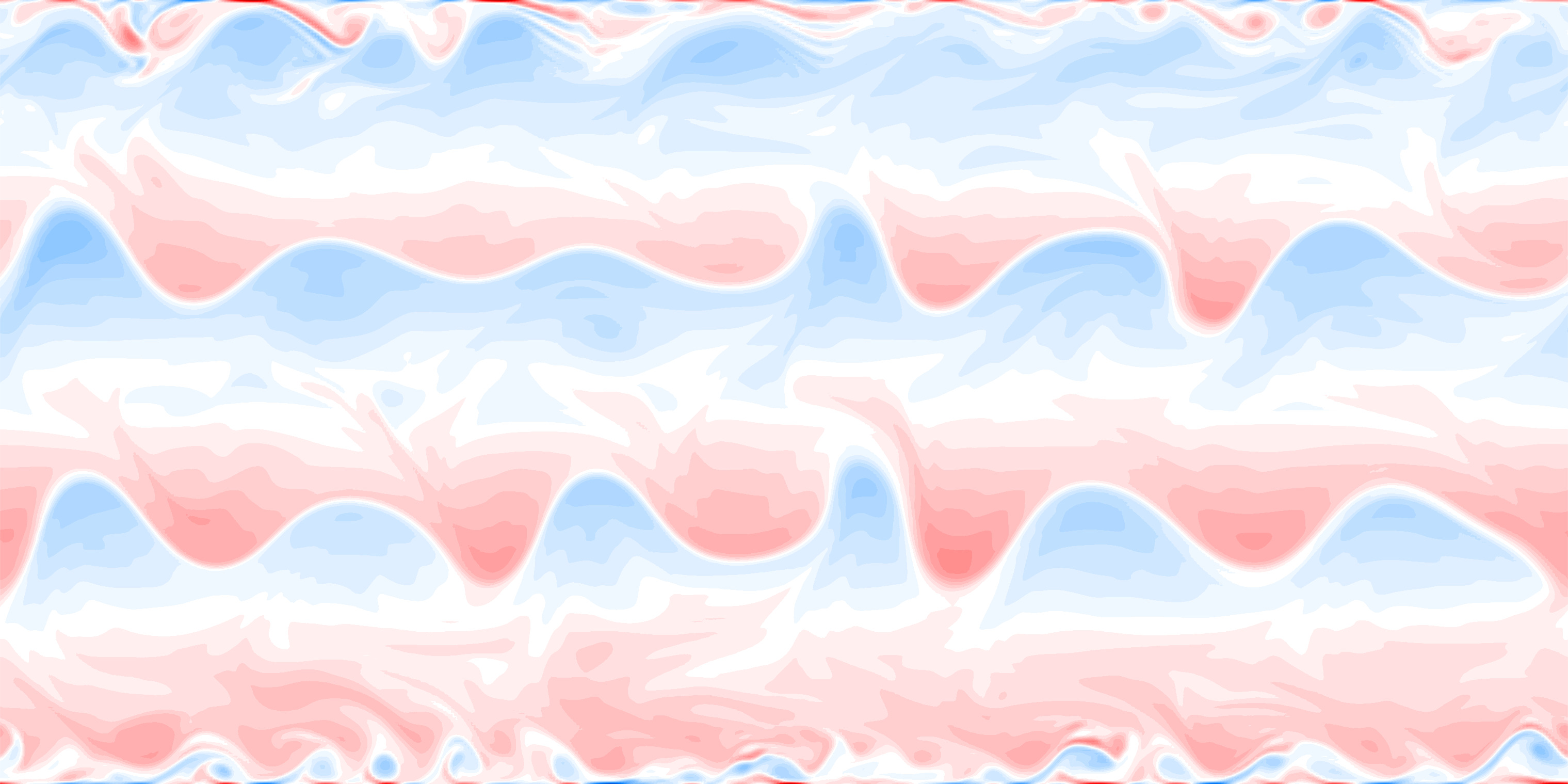
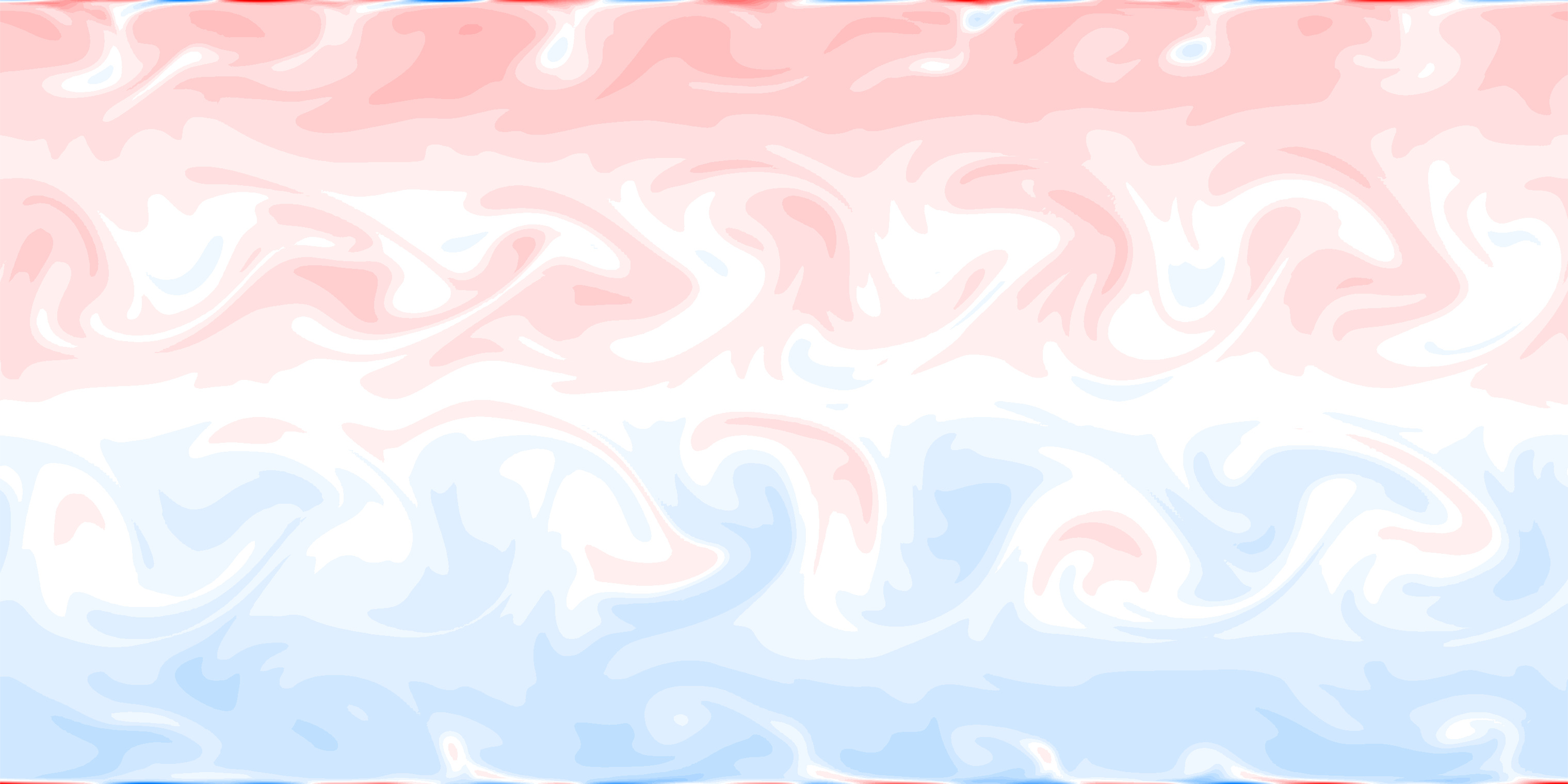
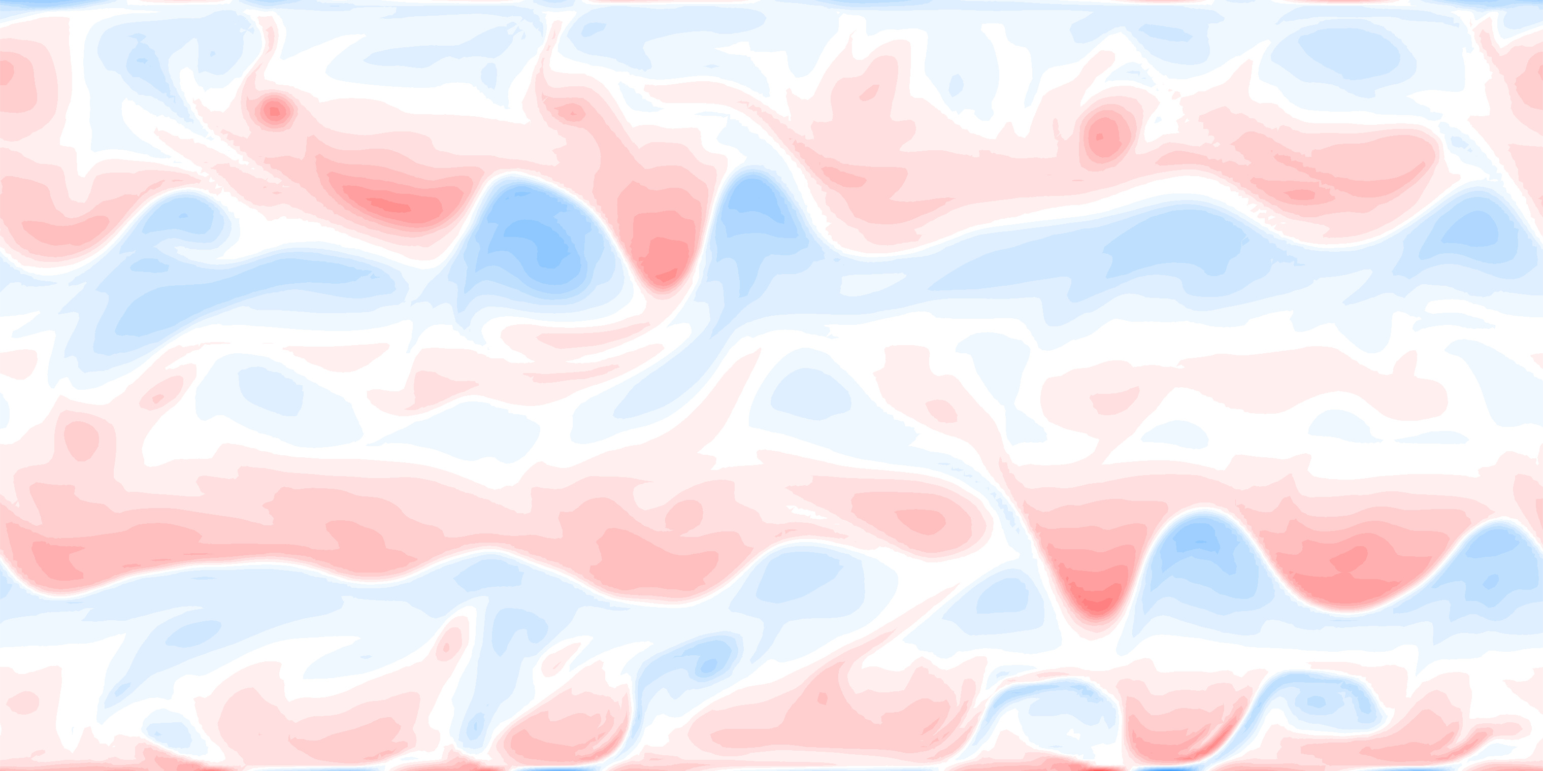
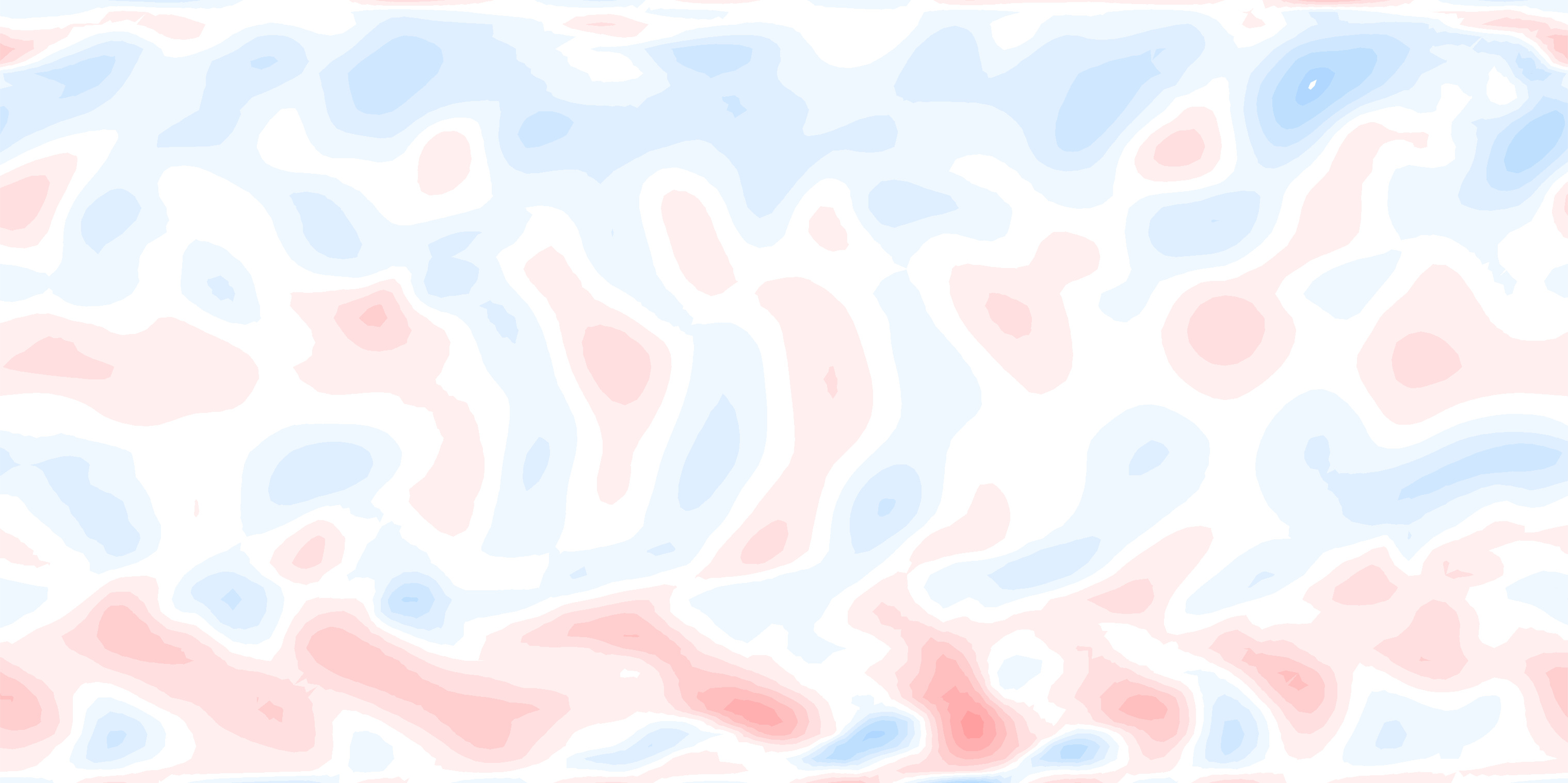
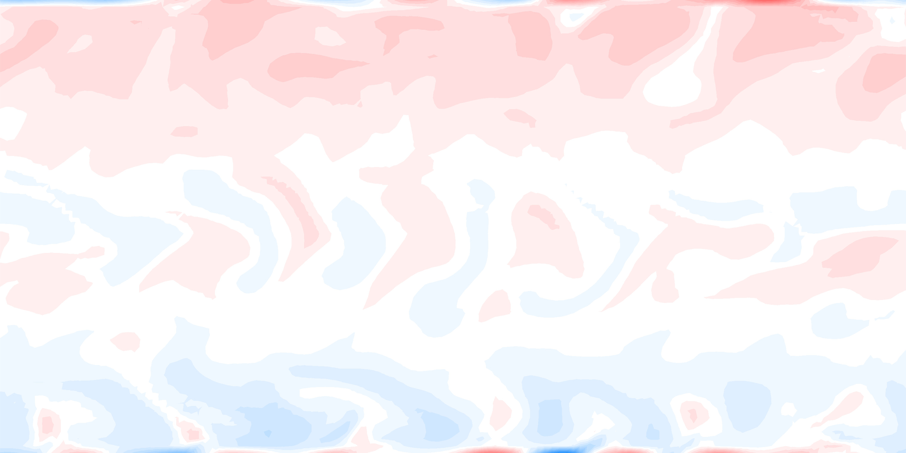
We consider a horizontally periodic flat-bottom channel $\Omega=[0,L_{x}]\times[0,L_{y}]\times[0,H]$ with $L_{x}=3840\,\rm km$, $L_{y}=L_{x}/2\,\rm km$, and total depth $H=H_{1}+H_{2}$, with $H_{1}=1.0\,\rm km$, $H_{2}=3.0\,\rm km$. The governing parameters of the QG model are typical to a mid-latitude setting, i.e. the planetary vorticity gradient $\beta=2\times 10^{-11}\,{\rm m^{-1}\,s^{-1}}$, lateral eddy viscosity $\nu=3.125\,\rm m^{2}s^{-1}$, and the bottom friction parameters $\mu=4\times 10^{-8}$. The background-flow zonal velocities in (20) are given by $U=[6.0,0.0]\,\rm cm\,s^{-1}$, and the stratification parameters in (21) are $s_{1}=4.22\cdot 10^{-3}\,\rm km^{-2}$, $s_{2}=1.41\cdot 10^{-3}\,\rm km^{-2}$; chosen so that the first Rossby deformation radius is $Rd_{1}=25\,{\rm km}$. In order to ensure that the numerical solutions are statistically equilibrated, the model is initially spun up from the state of rest to $t=0$ over the time interval $T_{spin}=[-50,0]\,{\rm years}$. The numerical solutions of the deterministic QG model (19) at different resolutions are presented in Fig. 1.

FIRST LAYER		SECOND LAYER
(a) $G=2049\times 1025$
		$\color[rgb]{1,1,1}q^{f}_{2}$
(b) $G=1025\times 513$
		$\color[rgb]{1,1,1}q^{f}_{2}$
(c) $G=513\times 257$
		$\color[rgb]{1,1,1}q^{f}_{2}$
(d) $G=257\times 129$
		$\color[rgb]{1,1,1}q^{f}_{2}$
(e) $G=129\times 65$
		$\color[rgb]{1,1,1}q^{f}_{2}$

Figure 1: The series of snapshots of PV anomaly $q$ shows the dependence of the solution on the resolution. All the fields are given in units of $[s^{-1}f^{-1}_{0}]$, where $f_{0}=0.83\times 10^{-4}\,{\rm s^{-1}}$ is the Coriolis parameter. In order to visualize all the solutions on the same color scale we have multiplied the ones in the second layer by a factor of 5.

We would like to draw the reader’s attention to the fact that the solution significantly depends on the resolution (see Fig. 1). Namely, the number of jets for the highest resolution $2049\times 1025$ (Fig. 1a) is four (four red striations in the interior of the computational domain; the boundary layers on the top and bottom boundaries are not counted as such). However, there are only two jets for the lower-resolution flows: $G=1025\times 513$ (Fig. 1b), $G=513\times 257$ (Fig. 1c), $G=257\times 129$ (Fig. 1d). Moreover, the lowest resolution flow (computed on the grid $G=129\times 65$, Fig. 1e) shows no jets at all, and this is the flow that we paramaterise and then apply the data assimilation methods described above. We also use a finer grid $G=257\times 129$ to study the effect of the resolutions on the data assimilation methods. It is important to note that there is no smooth transition between solutions at different resolutions like, for instance, in the double-gyre problem (e.g. SB2015 ), and this makes lower-resolution solutions much harder to parameterise, since the parameterisation should compensate not only for the information lost because of coarse-graining, but also for the missing physical effects. For example, in the channel flow, the backscatter mechanism (e.g, SB2016 ) at low resolutions is very weak, and thus it is not capable of cascading energy up to larger scales to maintain the jets.

In the following, we compare the dependence of the performance of the various procedures discussed above on the following parameters: the resolution of the signal grid, the number of observations (also referred to as weather stations), and the size of the data assimilation step. The methods will be applied to the parameterised QG model (25) which has been studied at length in CCHWS2019_2 .

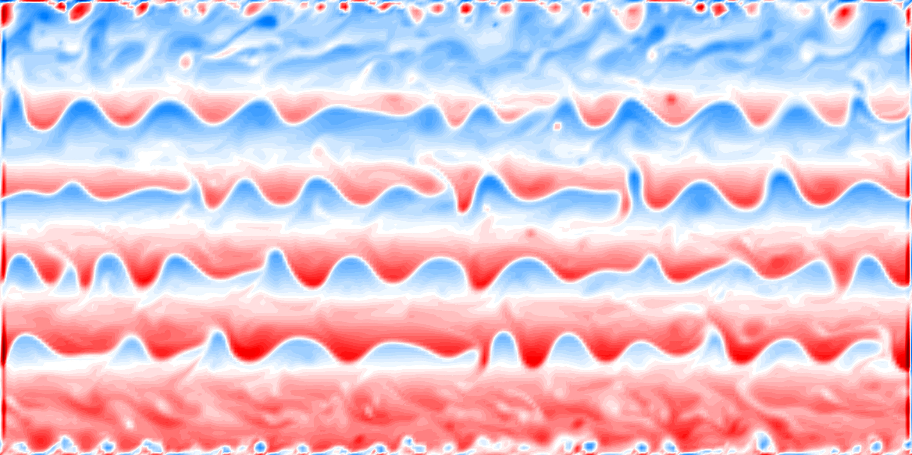
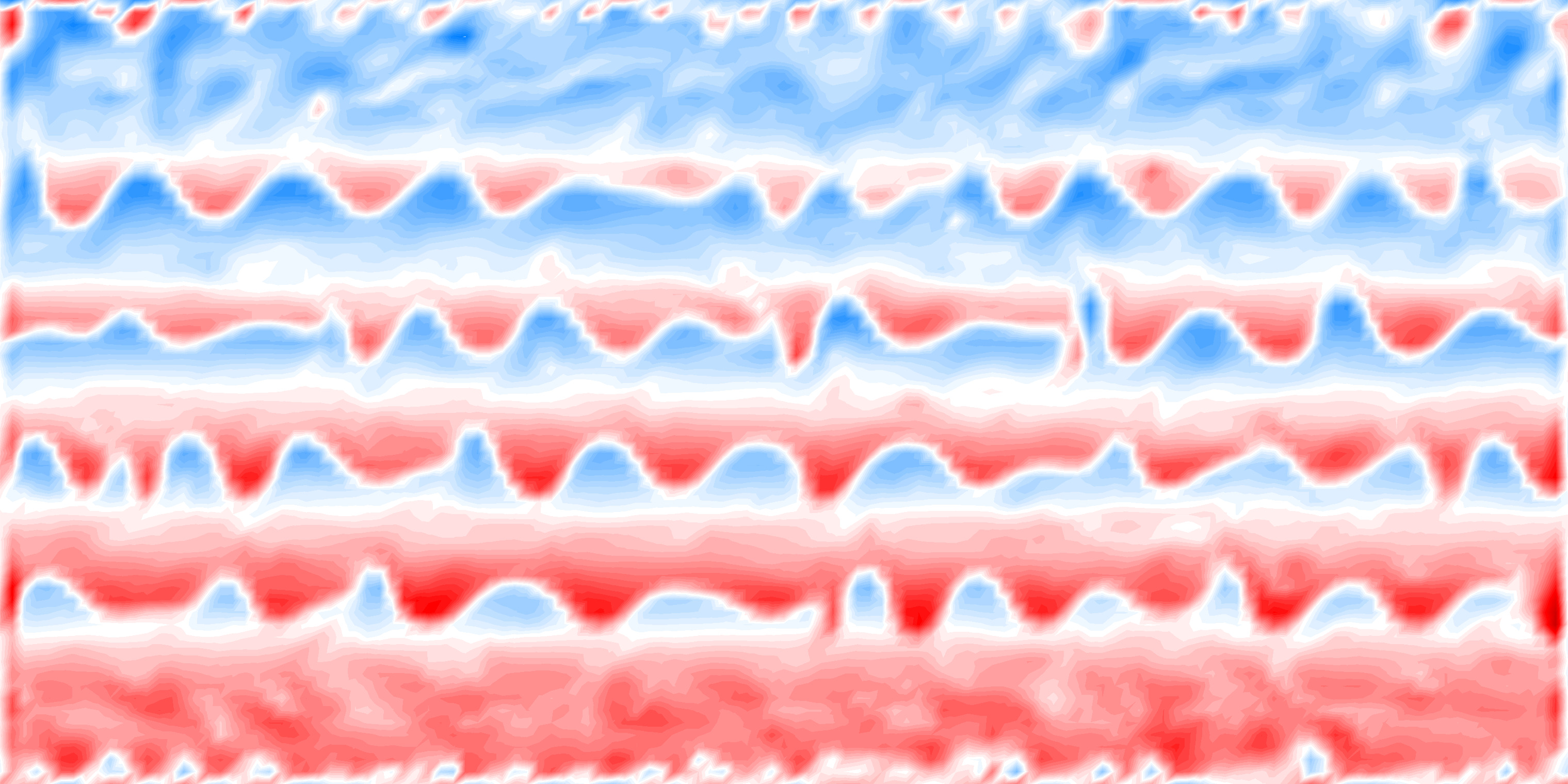
Before going into further details, we remind the reader how we compute the true solution, which is denoted as $q^{a}$, and also referred to as the truth or the the true state. For the purpose of this paper, we have computed two versions of the true solution $q^{a}$. The first one is computed on a signal grid $G_{s}=257\times 129$ ($dx\approx dy\approx 15\,{\rm km}$), and the other one is computed on a signal grid $G_{s}=129\times 65$ ($dx\approx dy\approx 299\,{\rm km}$) (Fig. 2). Each true solution is computed as the solution of the elliptic equation (21) with the stream function $\psi^{a}$, where $\psi^{a}$ is computed by spatially averaging the high-resolution stream function $\psi^{f}$ (computed on the fine grid $G_{f}=2049\times 1025,\,dx\approx dy\approx 1.9\,{\rm km}$) over the coarse grid cell $G^{s}$. From now on, we focus only on the first layer, since the flow in the first layer is more energetic and exhibits an interesting dynamics including small-scale vortices and large-scale zonally elongated jets.

	$G_{s}=257\times 129$	$G_{s}=129\times 65$
$q^{a}_{1}$

Figure 2: Shown is the true solution $q^{a}$ in the first layer computed on the grids $G_{s}=257\times 129$ (left) and $G_{s}=129\times 65$ (right). All the fields are given in units of $[s^{-1}f^{-1}_{0}]$, where $f_{0}=0.83\times 10^{-4}\,{\rm s^{-1}}$ is the Coriolis parameter.

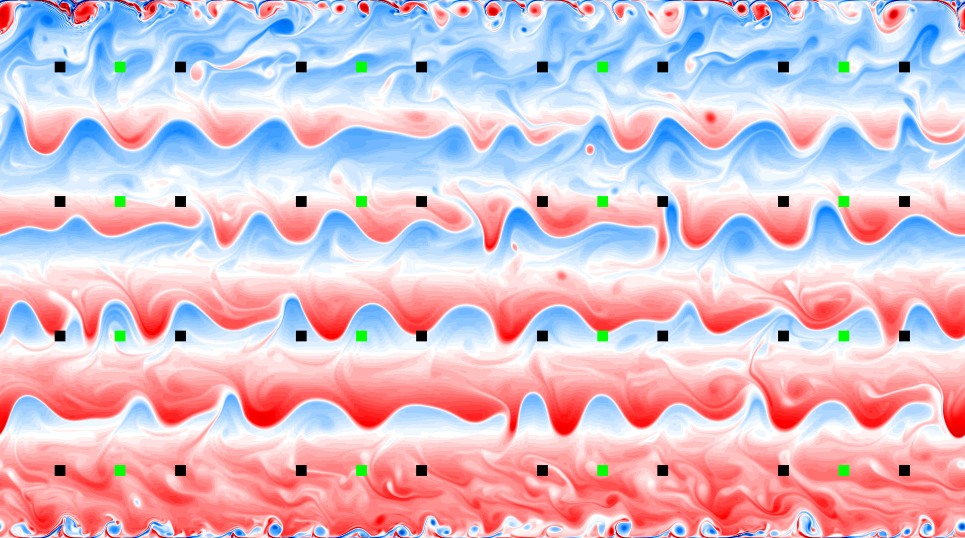
In order to study how the number of weather stations influences the accuracy of data assimilation methods we will consider two different setups including $M=16$ and $M=32$ weather stations. Clearly, the location of weather stations can be optimized in such a way so as to give the most accurate data assimilation results. For the purpose of this work, we locate the weather stations at the nodes of equidistant Eulerian grids $G_{d}=\{4\times 4,8\times 4\}$ shown in Fig. 3. In all numerical experiments we use $N=100$ particles (ensemble members) and $K=32$ (the number of $\xi$’s); the choice of these parameters has been justified in CCHWS2019_2 . It is worth noting that the initial conditions for the stochastic model have been computed over the spin up period $T_{\rm spin}=[-8,0]$ hours. The method of computing physically consistent initial conditions for the stochastic model is given in CCHWS2019_2 .

Figure 3: Snapshot of PV anomaly $q^{f}_{1}$ and location of weather stations for the data grids $G_{d}=\{4\times 4\}$ (green squares) and $G_{d}=\{8\times 4\}$ (black squares); the PV anomaly field is given in units of $[s^{-1}f^{-1}_{0}]$, where $f_{0}=0.83\times 10^{-4}\,{\rm s^{-1}}$ is the Coriolis parameter.

6.1 Tempering and jittering

We start with the study to the data assimilation algorithm that uses tempering and jittering, but not nudging (Algorithm 4). In the first experiment we run the stochastic QG model at the coarsest resolution ($G_{s}=129\times 65$) and use $M=16$ weather stations. We compare the results of the data assimilation methodology with the forward run of the stochastic model. For this experiment we take the data assimilation step to be $\Delta t=4$ hours (the data assimilation step is time between to consecutive analysis cycles.

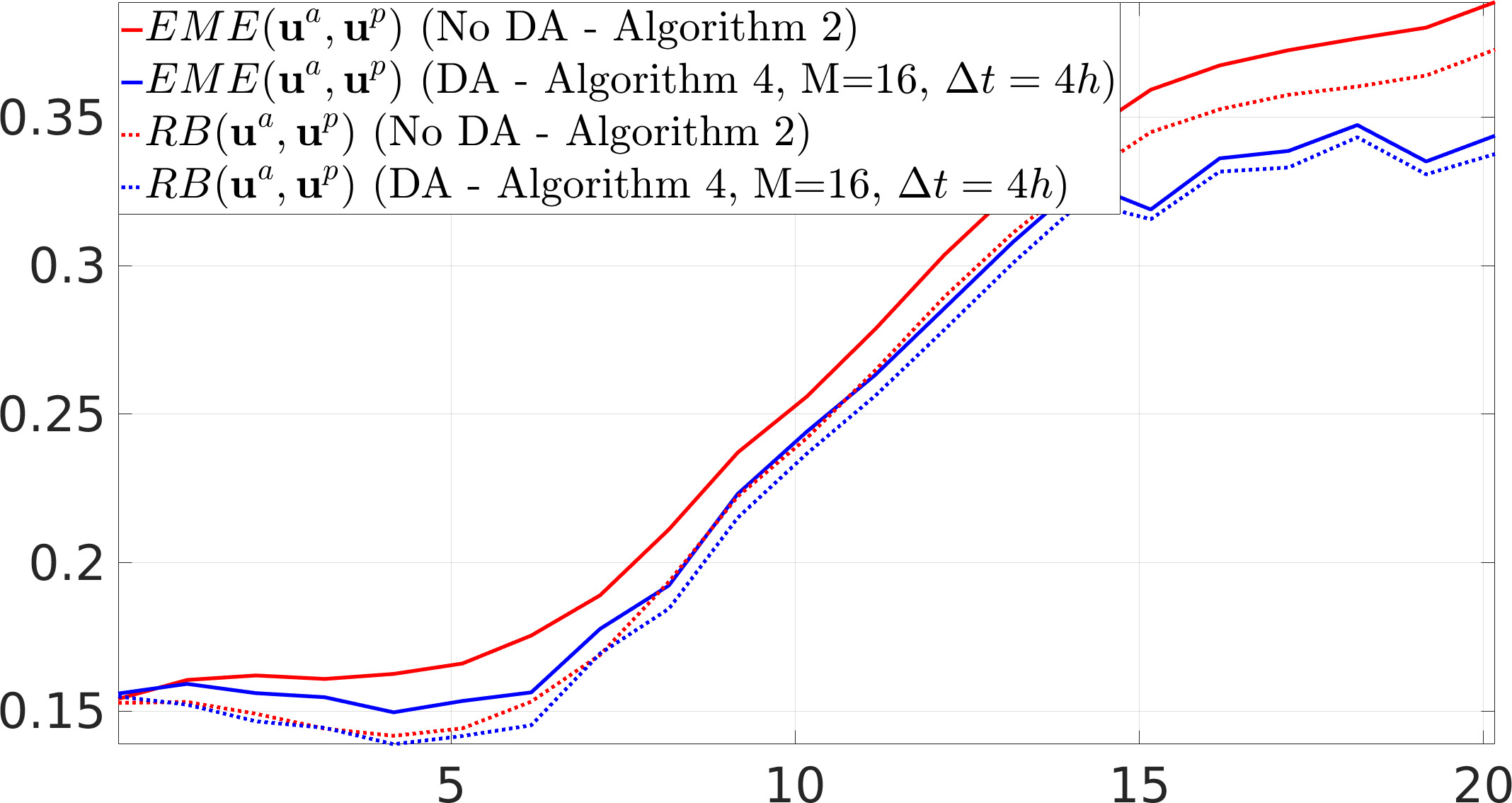
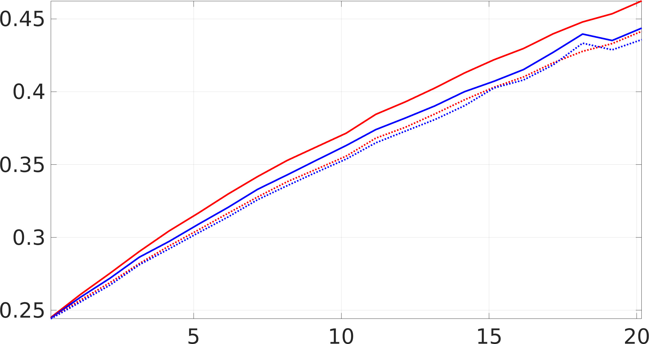
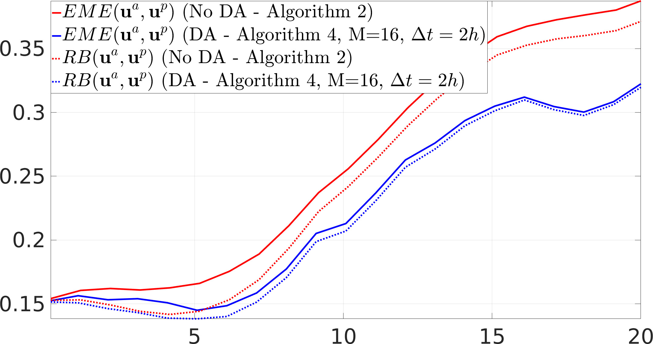
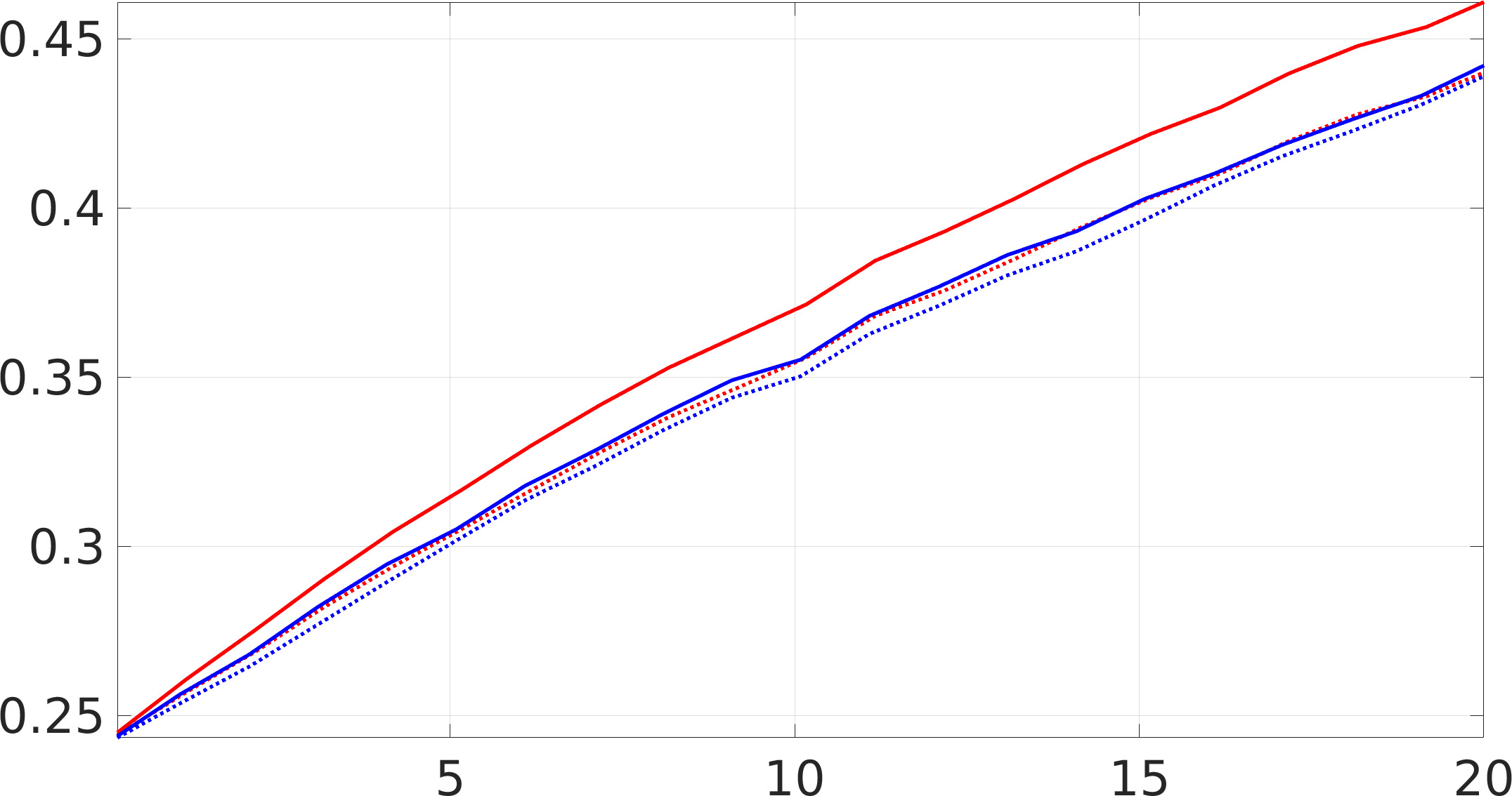
The results are presented in Fig. 4 in terms of the relative bias (RB) and the ensemble mean $l_{2}$-norm relative error (EME) given by

$$RB(\mathbf{u}^{a},\mathbf{u}^{p}) := \frac{\|\mathbf{u}^{a}-\bar{\mathbf{u}}^{p}\|_{2}}{\|\mathbf{u}^{a}\|_{2}},$$ (43)

$$EME(\mathbf{u}^{a},\mathbf{u}^{p}) := \frac{1}{N}\sum\limits^{N}_{n=1}\frac{\|\mathbf{u}^{a}-\mathbf{u}^{p}_{n}\|_{2}}{\|\mathbf{u}^{a}\|_{2}},$$ (44)

with $\mathbf{u}^{p}_{n}$ being the $n$-th member of the stochastic ensemble, $\mathbf{u}^{a}$ is the true solution, and $\displaystyle\bar{\mathbf{u}}^{p}:=\frac{1}{N}\sum\limits^{N}_{n=1}\mathbf{u}^{p}_{n}$.

	(a): EME for all weather stations	(b): EME for the whole domain
EME
	t [days]	t [days]

Figure 4: Evolution of the ensemble mean relative $l_{2}$-norm error (EME) and relative bias (RB) for (a) all weather stations and (b) the whole domain; $\mathbf{u}^{a}$ is the true solution, $\mathbf{u}^{p}$ is the stochastic solution. In order to assimilate data we use tempering and jittering (Algorithm 4); the data is assimilated from $M=16$ weather stations every 4 hours; the grid size is $G_{s}=129\times 65$.

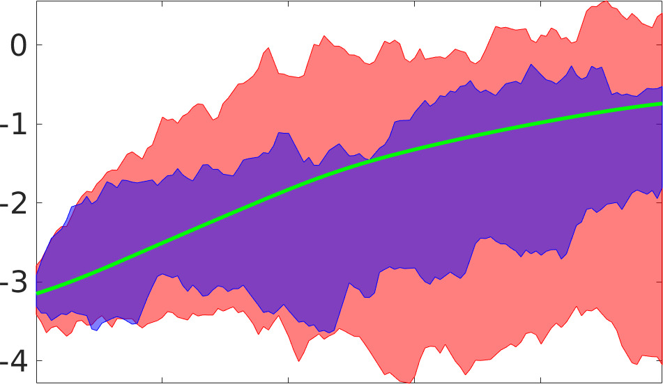
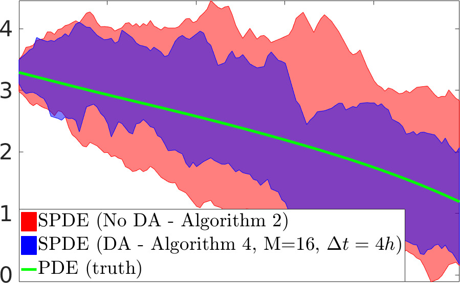
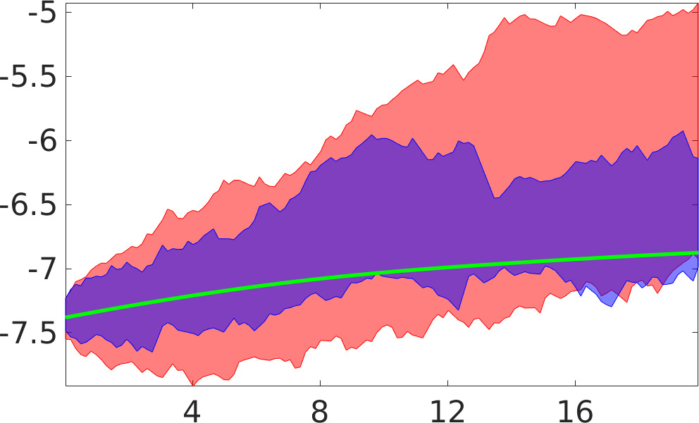
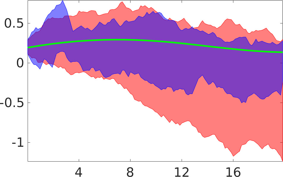
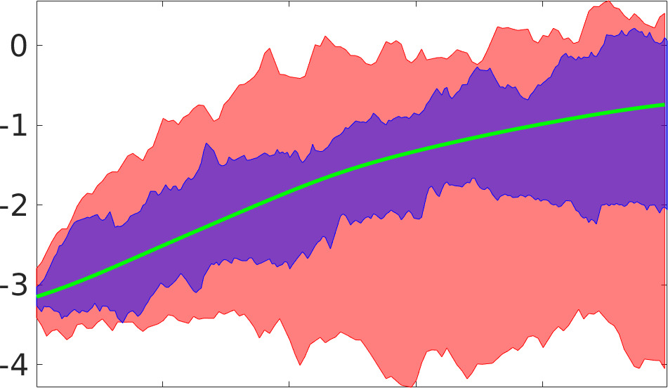
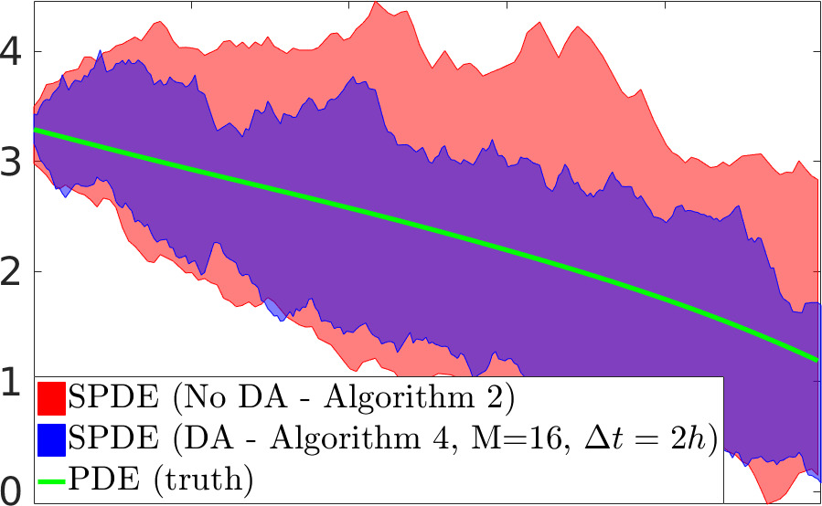
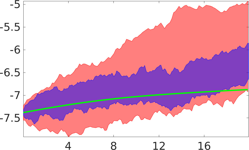
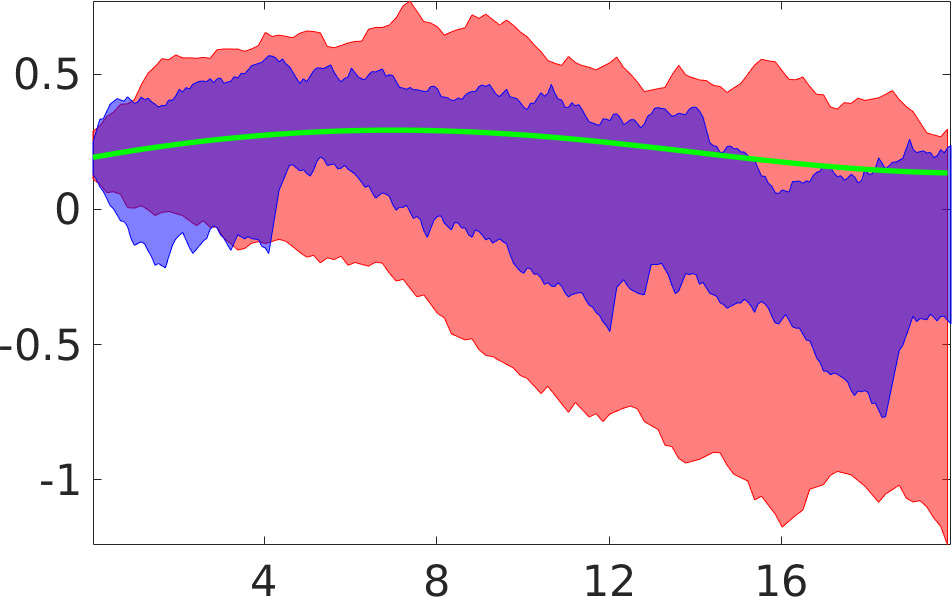
As Fig. 4 shows, the data assimilation method presented by Algorithm 4 (blue line) offers little improvement over the SPDE run without data assimilation methodology (red line) both in terms of the relative bias and in terms of the EME at the weather stations (Fig. 4a) and in the whole domain (Fig. 4b) throughout the time period of 20 days. As we will see later, the situation will improve as we decrease the data assimilation step and/or increase the resolution of the signal grid. But before, let us first look at the uncertainty quantification results for this particular setting. As expected, the spread for the stochastic QG model (25) decreases (to a certain extend) after the application of the data assimilation methodology. We illustrate the shrinkage of the stochastic spreads in Fig. 5 for the velocity computed at weather stations located in the slow flow region (blue stripes) and fast flow region (red jets) in Fig. 3.

$u^{p}_{1}$	$v^{p}_{1}$
t [days]	t [days]

Figure 5: Shown are typical stochastic spreads for velocity $\mathbf{u}^{p}_{1}=(u^{p}_{1},v^{p}_{1})$ at weather stations located in the slow flow region (upper row) and fast flow region (lower row); the grid size is $G_{s}=129\times 65$.

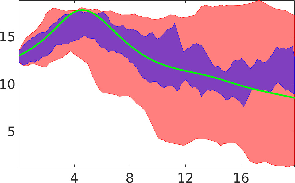
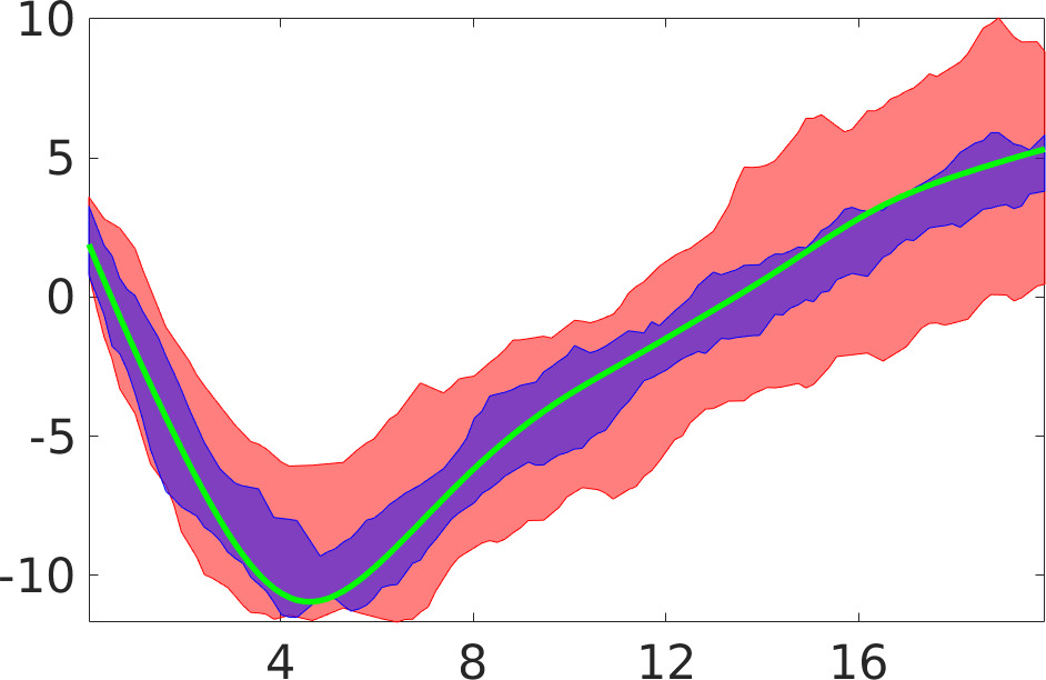
Fig. 5 shows that the truth (green line) is contained within the stochastic spread computed with and without the data assimilation method. Moreover, the spread computed with the data assimilation method (blue spread) is narrower than that computed only with the SPDE (red spread). To reduce it further, one can vary the data assimilation step $\Delta t$. In particular, halving $\Delta t$ brings further reduction in both RB and EME (Fig. 6) and also reduces the uncertainty of the stochastic solution (Fig. 7) (the spread is narrower).

	(a): EME for all weather stations	(b): EME for the whole domain
EME
	t [days]	t [days]

Figure 6: The same as in Fig. 4, but for the data assimilation step $\Delta t=2h$.

$u^{p}_{1}$	$v^{p}_{1}$
t [days]	t [days]

Figure 7: The same as in Fig. 5, but for the data assimilation step $\Delta t=2h$.

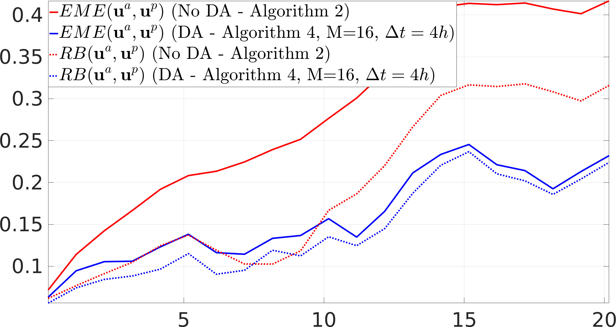
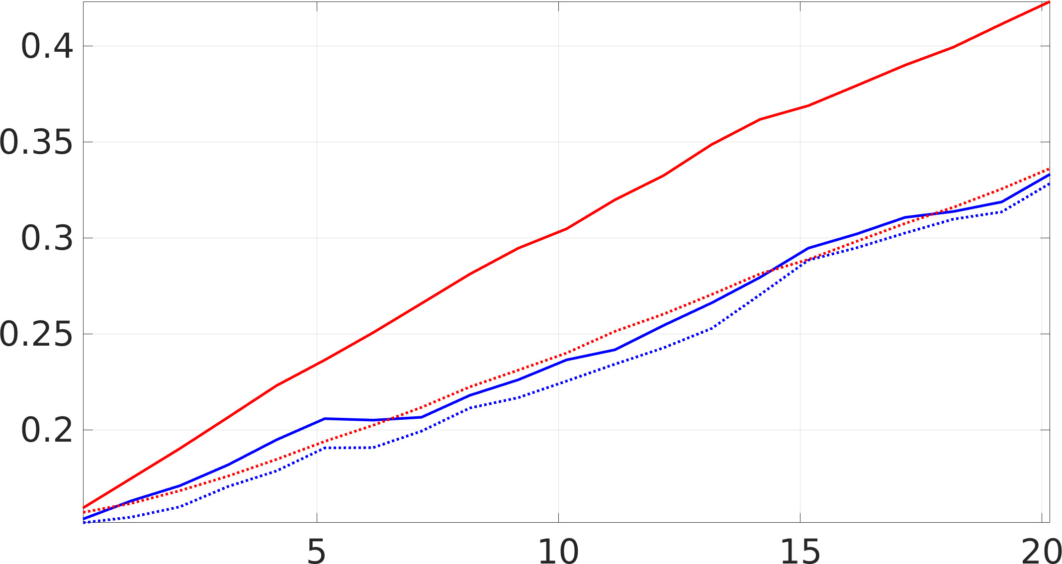
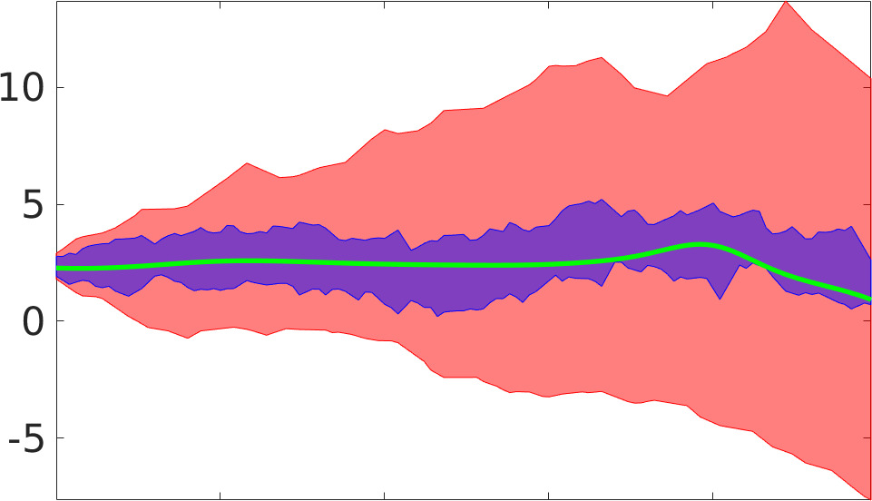
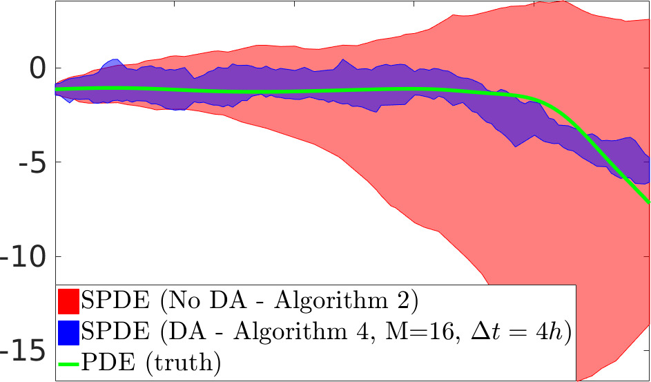
Further substantial improvements in the performance of the data assimilation methodology are obtained when the resolution of the signal grid gets higher ($G_{s}=257\times 129$). In particular, the results are much more accurate both at the observation points (weather stations) (Fig. 8a) and over the whole domain (Fig. 8b). Moreover, the spread of the sample reduces dramatically as shown in figure Fig. 9.

	(a): EME for all weather stations	(b): EME for the whole domain
EME
	t [days]	t [days]

Figure 8: The same as in Fig. 4, but for the signal grid $G_{s}=257\times 129$.

$u^{p}_{1}$	$v^{p}_{1}$
t [days]	t [days]

Figure 9: The same as in Fig. 5, but for the signal grid $G_{s}=257\times 129$.

Based on the above results, we conclude that both the reduction of the data assimilation step and the increase of the resolution of the signal grid can enhance the accuracy of the stochastic solution and reduce the spread of the stochastic ensemble. The effect of the increase of the resolution on both the accuracy and uncertainty appears to be much more pronounced compared to that of the reduction of the data assimilation step.

6.2 Nudging

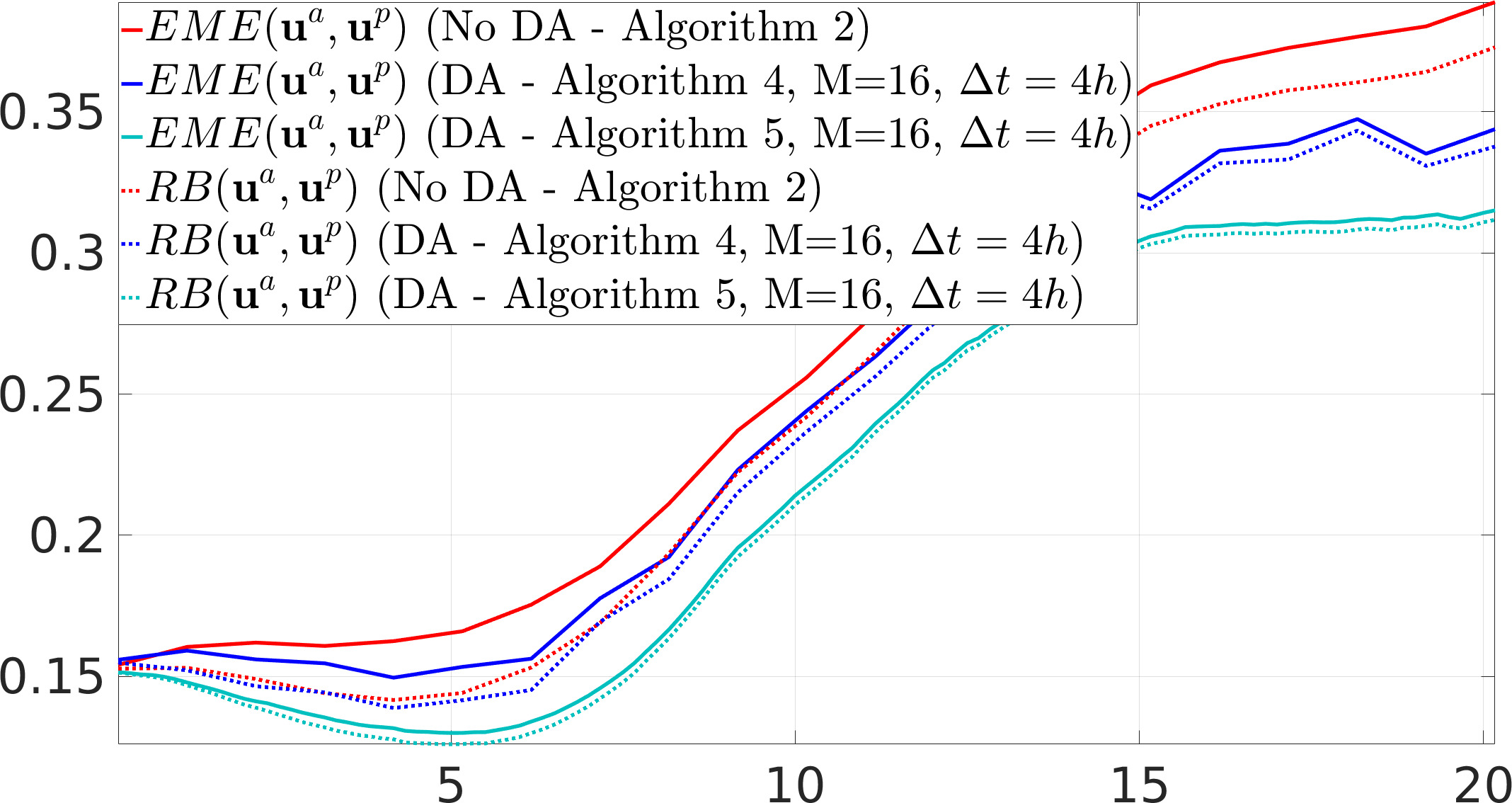
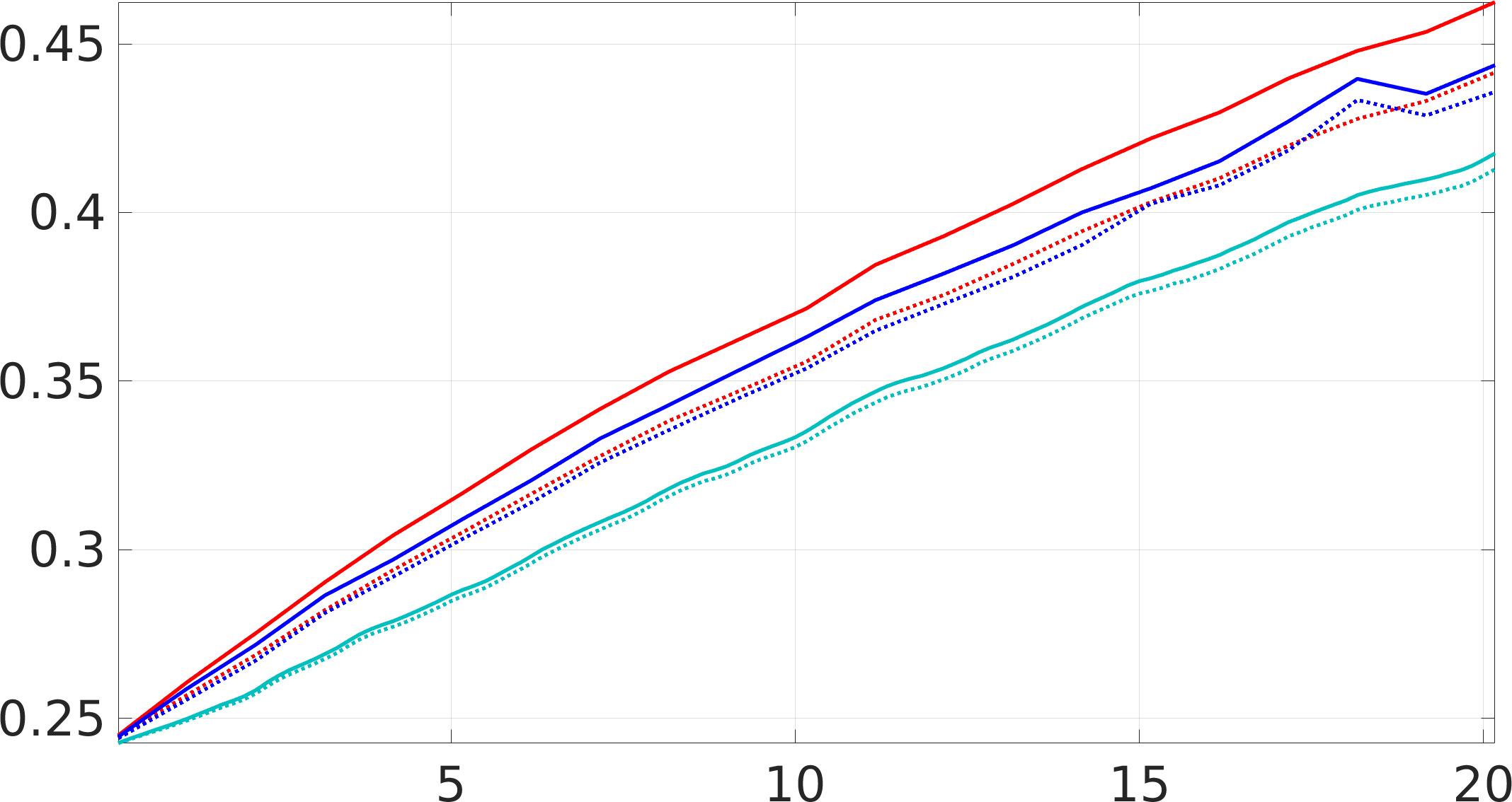
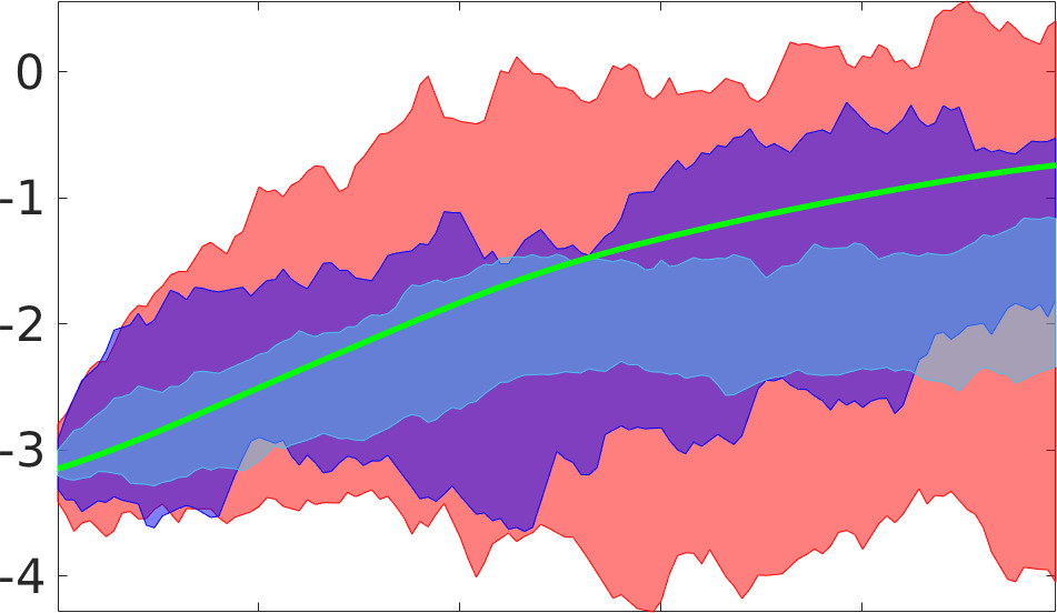
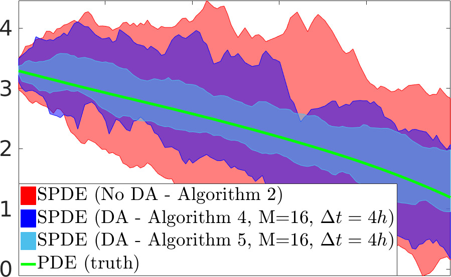
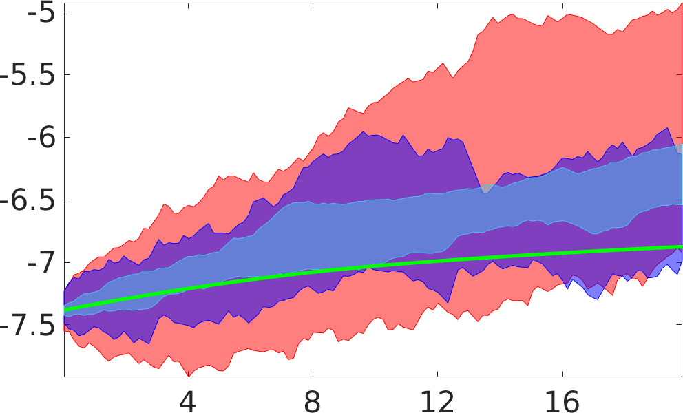
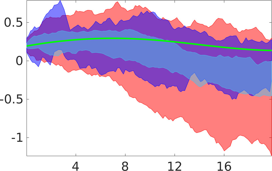
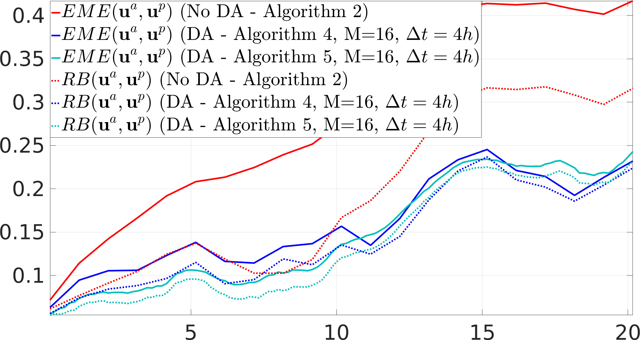
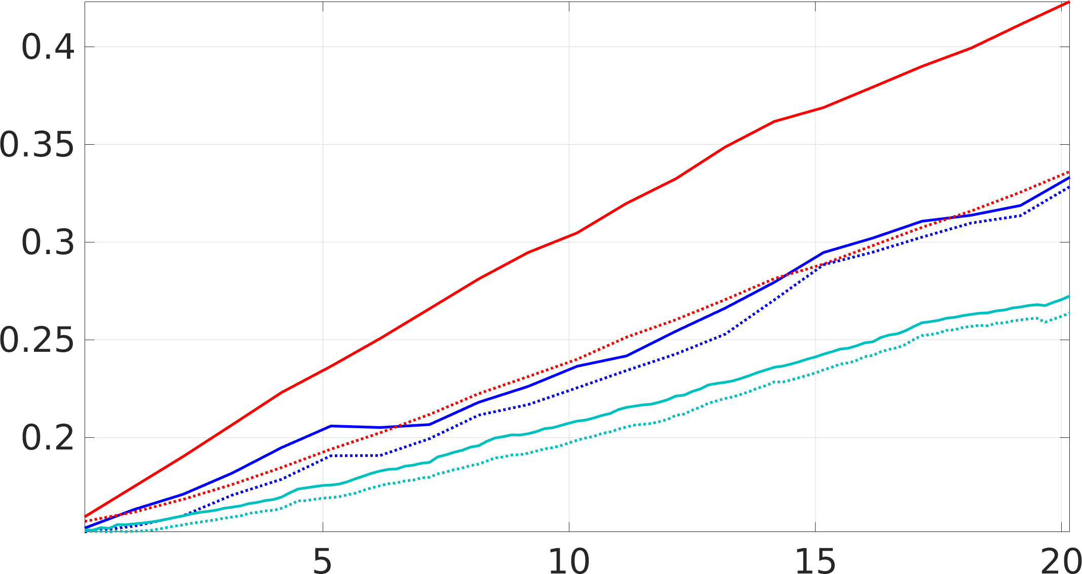
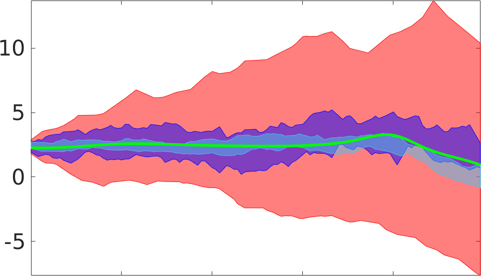
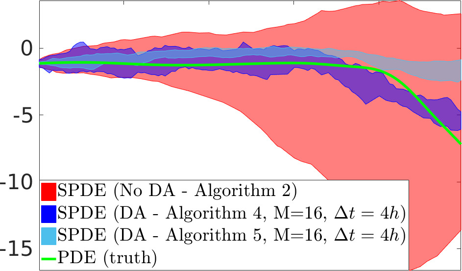
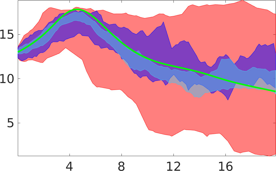
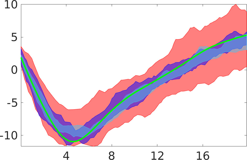
We will now look at the performance of the data assimilation methodology that includes nudging (Algorithm 5) compared with the one that does not (Algorithm 4). As above we start with the stochastic QG model at the coarsest resolution ($G_{s}=129\times 65$) and use $M=16$ weather stations. We present the results in Figs. 10 and 11. The improvements are obvious straightaway. The average of the stochastic spread becomes closer to the true solution compared with the same case but without using the nudging procedure (Fig. 10). However, in some cases, the true solution leaves the spread of the ensemble (Fig. 11). We do not have a clear explanation for this behaviour.

	(a): EME for all weather stations	(b): EME for the whole domain
EME
	t [days]	t [days]

Figure 10: Evolution of the ensemble mean relative $l_{2}$-norm error (EME) and relative bias (RB) for (a) all weather stations and (b) the whole domain; $\mathbf{u}^{a}$ is the true solution, $\mathbf{u}^{p}$ is the stochastic solution. In order to assimilate data we use tempering, jittering, and nudging (Algorithm 5); the data is assimilated from $M=16$ weather stations every 4 hours; the grid size is $G_{s}=129\times 65$.

$u^{p}_{1}$	$v^{p}_{1}$
t [days]	t [days]

Figure 11: Shown are typical stochastic spreads of velocity $\mathbf{u}^{p}_{1}=(u^{p}_{1},v^{p}_{1})$ at weather stations located in the slow flow region (upper row) and fast flow region (lower row) for the SPDE without (red) and with (light blue) using tempering, jittering, and nudging (Algorithm 5); Algorithm 4 (blue) is given for ease of comparison. The green line is the true solution; the grid size is $G_{s}=129\times 65$.

Again, at the higher resolution ($G_{s}=257\times 129$), the nudged solution is even more accurate than its low-resolution version (Fig. 12), and the uncertainty is further reduced (Fig. 13).

	(a): EME for all weather stations	(b): EME for the whole domain
EME
	t [days]	t [days]

Figure 12: The same as in Fig. 10, but for the signal grid $G_{s}=257\times 129$.

$u^{p}_{1}$	$v^{p}_{1}$
t [days]	t [days]

Figure 13: The same as in Figure 11, but for the signal grid $G_{s}=257\times 129$.

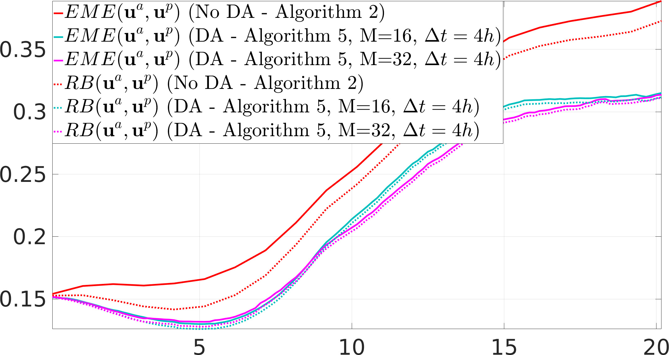
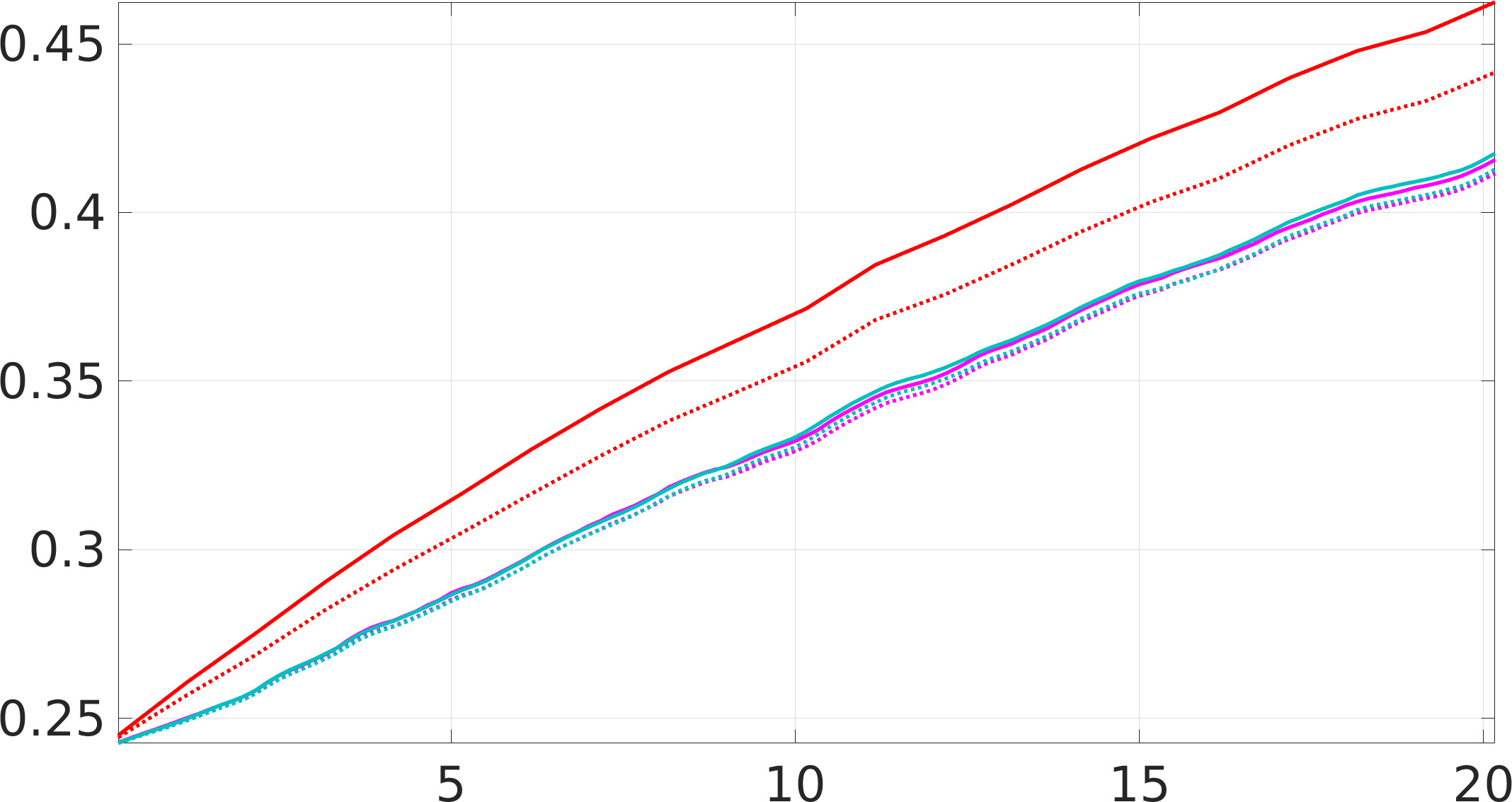
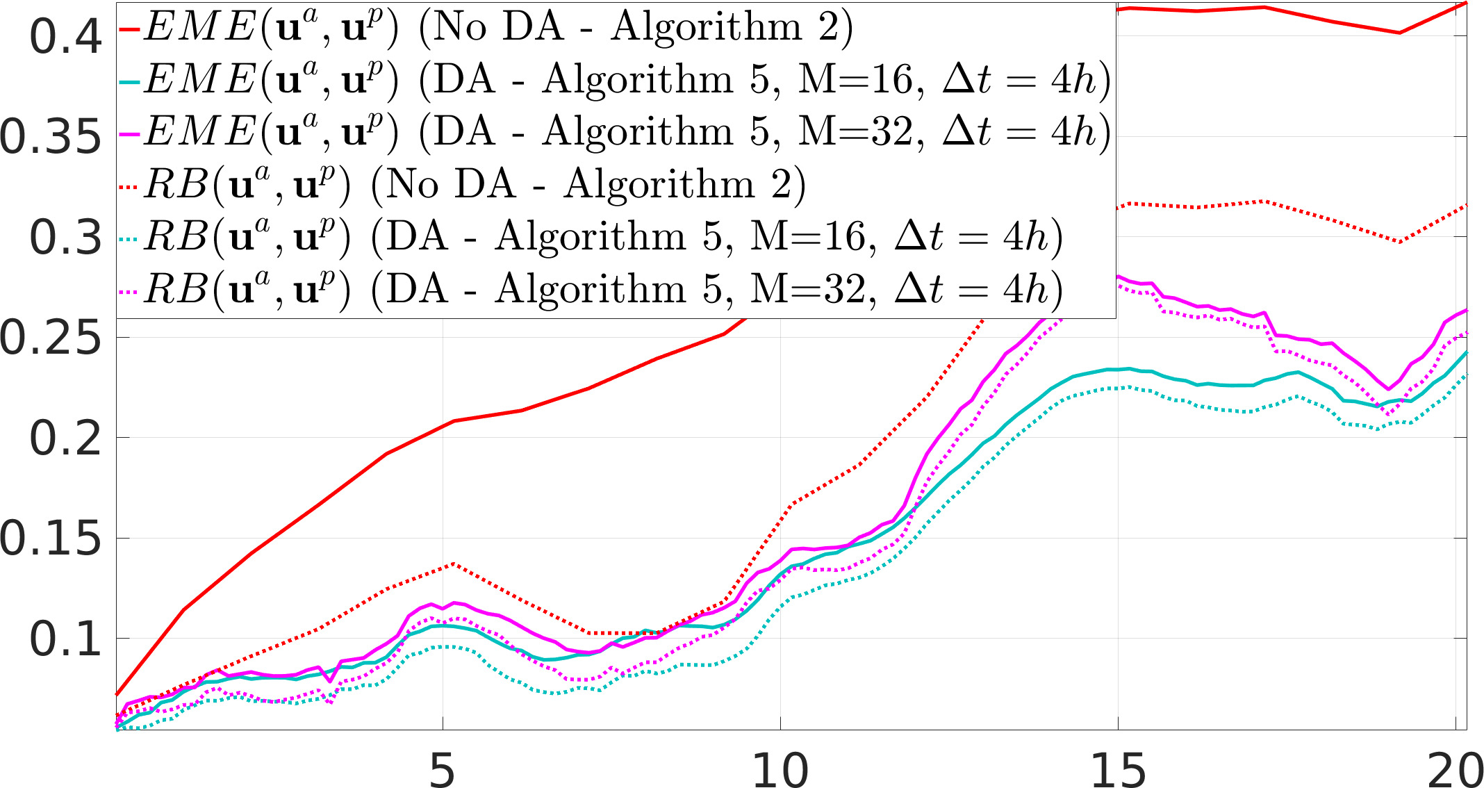
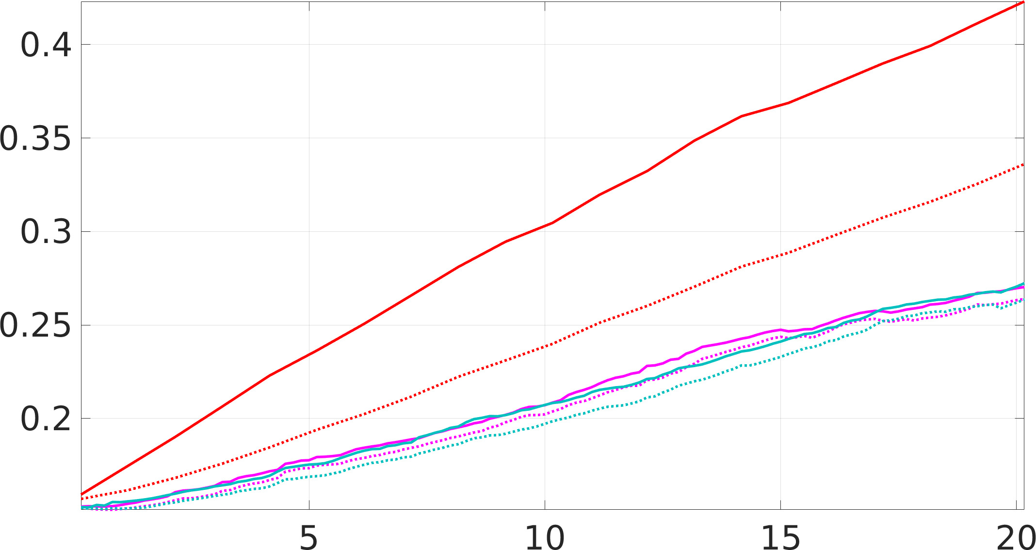
It is important to note that the number of observation locations (weather stations) used in the simulations above is only 0.19% and 0.05% of all degrees of freedom for the grids $G_{s}=129\times 65$ and $G_{s}=257\times 129$, respectively. Obviously, this number of weather stations is not enough to significantly reduce the uncertainty and decrease the error between the true solution and its parameterisation. Therefore, in the next simulation we double the number of observation locations ($M=32$) and compare how Algorithm 5 (data assimilation with the nudging method) performs when more observational data is available.

As can be seen in Fig. 14, adding more weather stations does not significantly influence the results for the low-resolution (Fig. 14) and higher-resolution (Fig. 14) simulation.

	(a): EME for all weather stations	(b): EME for the whole domain
EME
	t [days]	t [days]

Figure 14: Evolution of the ensemble mean relative $l_{2}$-norm error (EME) and relative bias (RB) for (a) all weather stations and (b) the whole domain; $\mathbf{u}^{a}$ is the true solution, $\mathbf{u}^{p}$ is the stochastic solution. In order to assimilate data we use tempering, jittering, and nudging (Algorithm 5); the data is assimilated from $M=32$ weather stations every 4 hours; the grid size is $G_{s}=129\times 65$.

	(a): EME for all weather stations	(b): EME for the whole domain
EME
	t [days]	t [days]

Figure 15: The same as in Figure 14, but for the signal grid $G_{s}=257\times 129$.

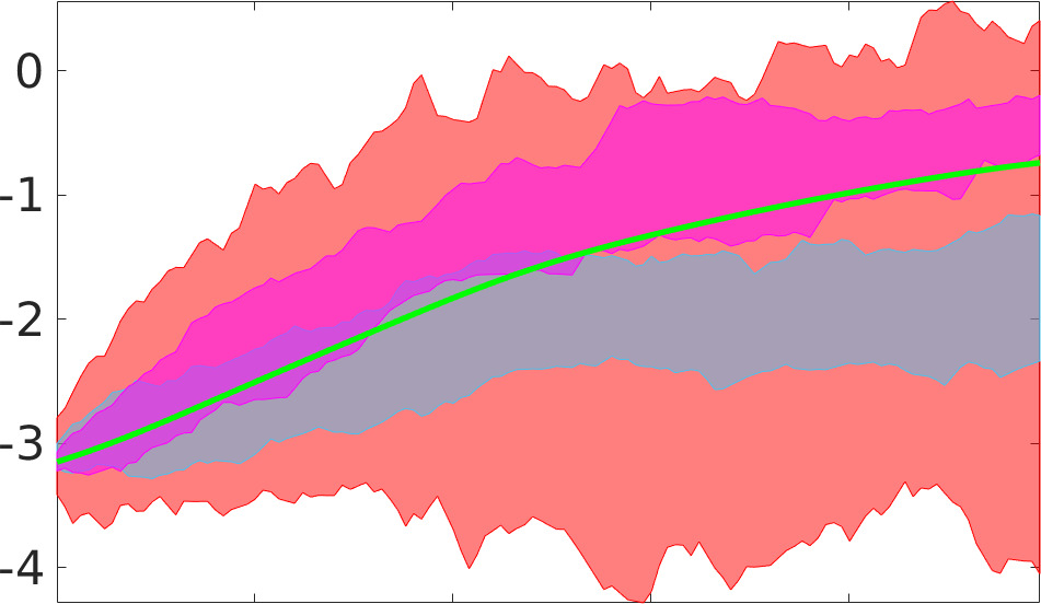
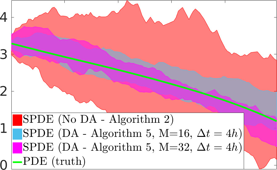
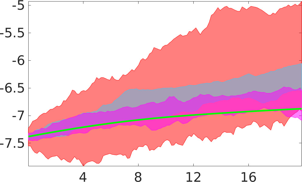
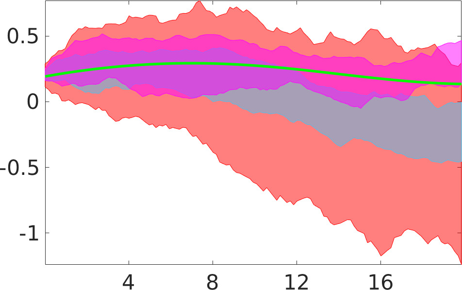
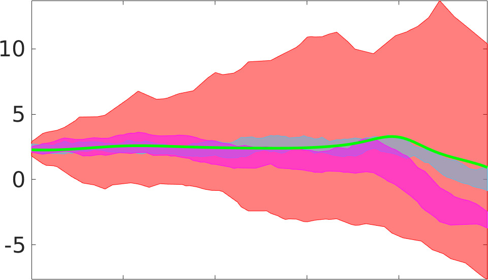
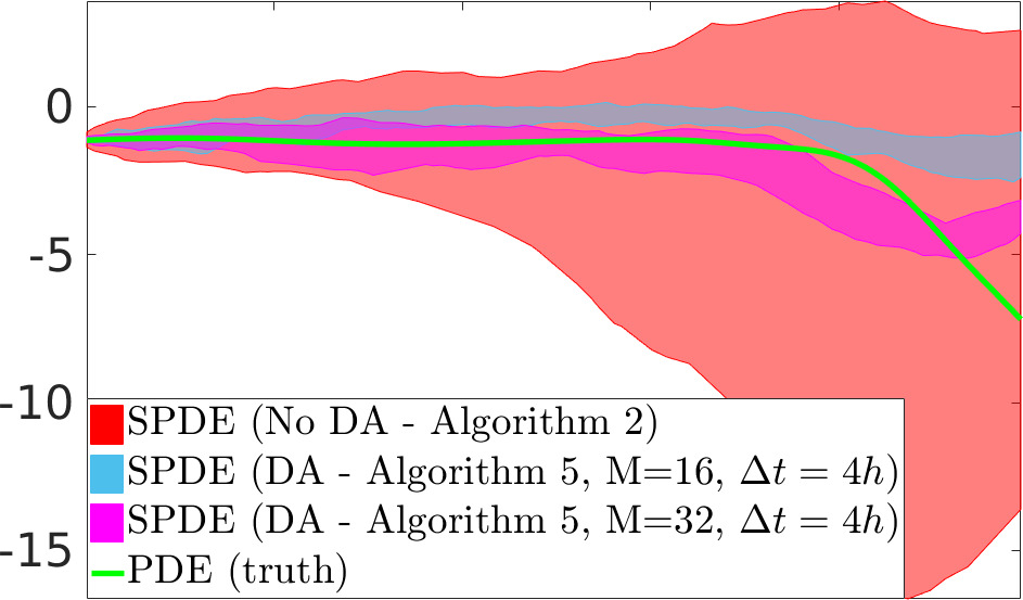
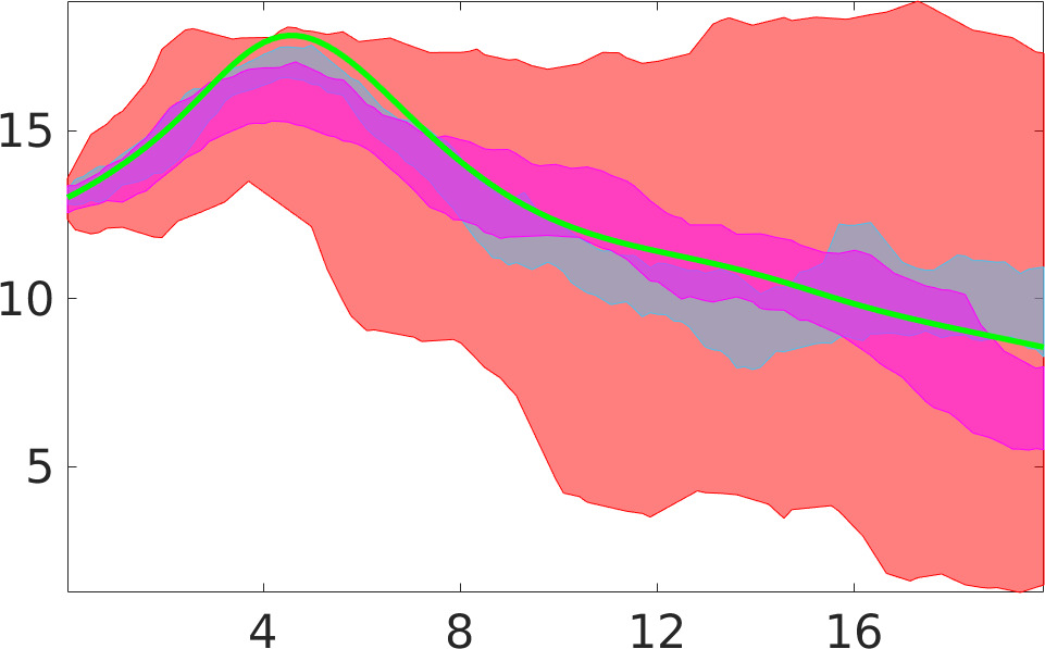
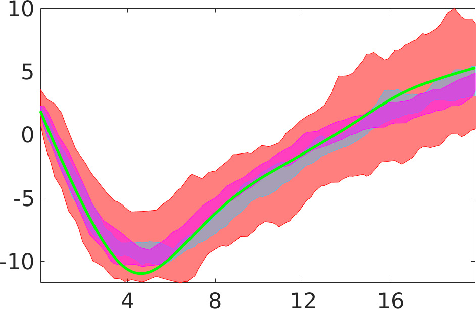
When more observational data is available (32 weather stations), the uncertainty of the stochastic solution remains virtually the same compared with the case of using 16 weather stations for both $G_{s}=129\times 65$ (Fig. 16) and $G_{s}=257\times 129$ (Fig. 17).

$u^{p}_{1}$	$v^{p}_{1}$
t [days]	t [days]

Figure 16: Shown are typical stochastic spreads of velocity $\mathbf{u}^{p}_{1}=(u^{p}_{1},v^{p}_{1})$ at the weather stations located in the slow flow region (upper row) and fast flow region (lower row) for the SPDE without (red) and with (blue) using tempering, jittering, and nudging (Algorithm 5). The green line is the true solution; the grid size is $G_{s}=129\times 65$.

$u^{p}_{1}$	$v^{p}_{1}$
t [days]	t [days]

Figure 17: The same as in Fig. 16, but for the signal grid $G_{s}=257\times 129$.

Again, we conclude that the Algorithm 4 improves the accuracy and reduces the uncertainty of the stochastic spread. The three parameters that we studied, the data assimilation step, and the size of the grid and the number of weather station, influence the performance of the data assimilation methodology. In particular, the smaller the data assimilation step is, the higher the accuracy becomes. We have found that the number of weather stations has a minor effect on the accuracy. However, if the resolution of the signal grid increases so does the accuracy of the solution computed with using the data assimilation methodology. Moreover, increasing the resolution of the signal grid $G_{s}$ dramatically reduces the uncertainty. The same conclusions are true for the Algorithm 5 that incorporates the nudging method. Moreover, the nudging procedure gives even more accurate solutions and further reduces the spread when compared with Algorithm 4.

We have also assessed the ensemble reliability on the grid $G_{s}=257\times 129$ by analysing the rank histograms (see, e.g. Anderson1996 ) computed by simulating the stochastic model (without using the data assimilation methodology) (Fig. 18a) and compared them with the rank histograms for the ensemble produced by Algorithm 5 (Fig. 18b). As the plots show, the stochastic ensemble, computed without the regular corrections made through the data assimilation method, has a bias (rank histograms are not flat) at many observation locations. As a result it will makes the ensemble prediction unreliable.

$u^{p}_{1}$                   $v^{p}_{1}$	$u^{p}_{1}$                   $v^{p}_{1}$
(a) Rank histogram without data assimilation	(b) Rank histograms with data assimilation

Figure 18: Rank histograms for velocity $\mathbf{u}^{p}_{1}=(u^{p}_{1},v^{p}_{1})$ at six different locations (not shown). Three observation points are located in the fast flow within red jets (first three upper rows in the plot), and the other three observation points are located in the slow flow between the jets (next three rows in the plot). Each histogram is based on 500 forecast-observation pairs generated by solving the stochastic QG model without (a) and with (b) using data assimilation. For simulating the stochastic QG model we use $N=100$ (ensemble size), $K=32$ (number of $\xi$’s); for the data assimilation method we use Algorithm 5 (tempering, jittering, and nudging), the number of observation locations $M=32$, the data assimilation step $\Delta t=4h$. Each ensemble member for the rank histogram is selected randomly from the ensemble of 100 members every 4 hours.

The situations changes when one uses the data assimilation method based one tempering, jittering, and nudging (Algorithm 5); see Fig. 18b. All the rank histograms now show no sign of a pronounced bias and demonstrate a well-calibrated ensemble. In other words, the application of the data assimilation methodology proposed in the paper corrects the bias introduced by the paramaterisation and produces a reliable forecast.

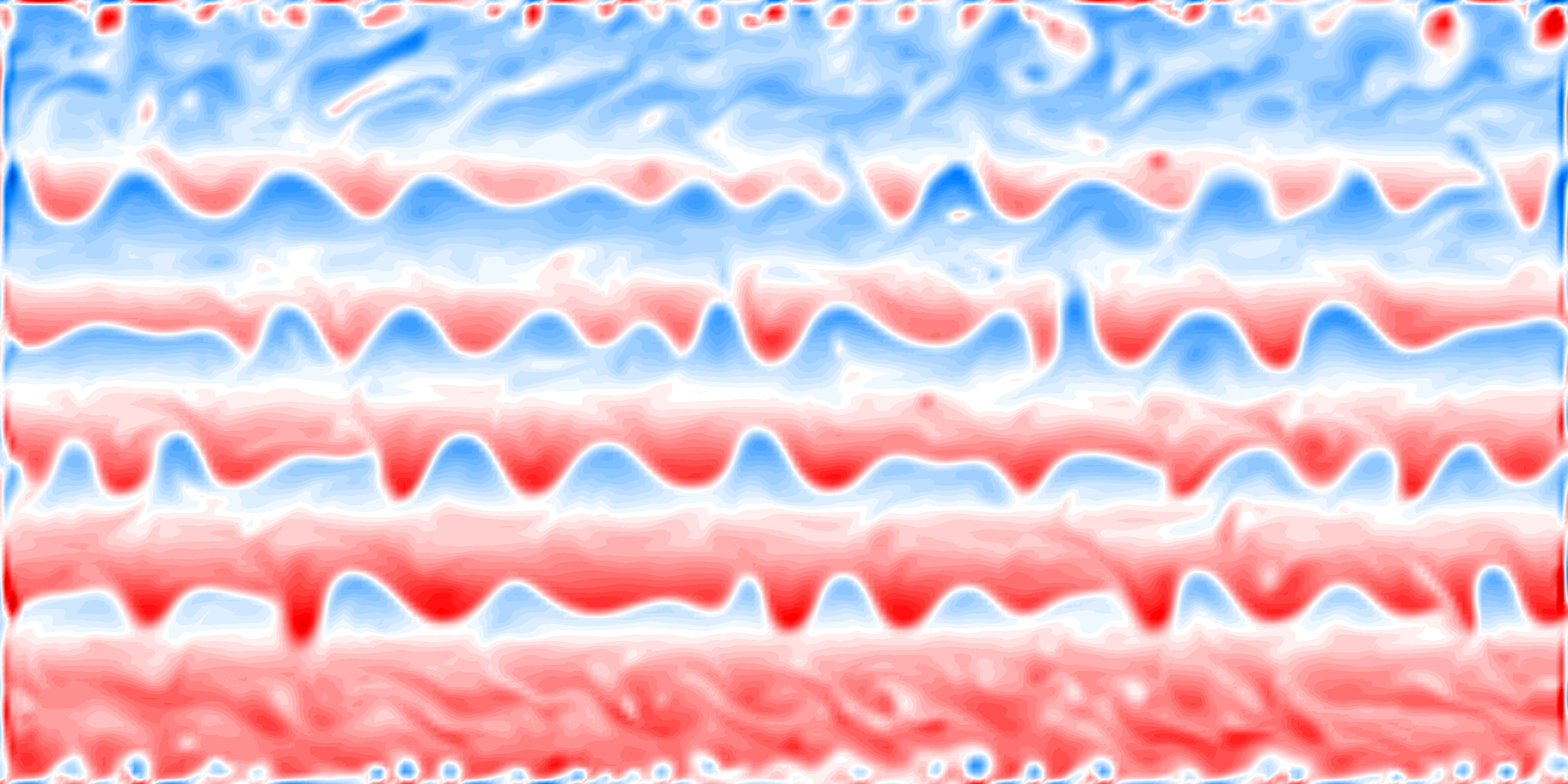
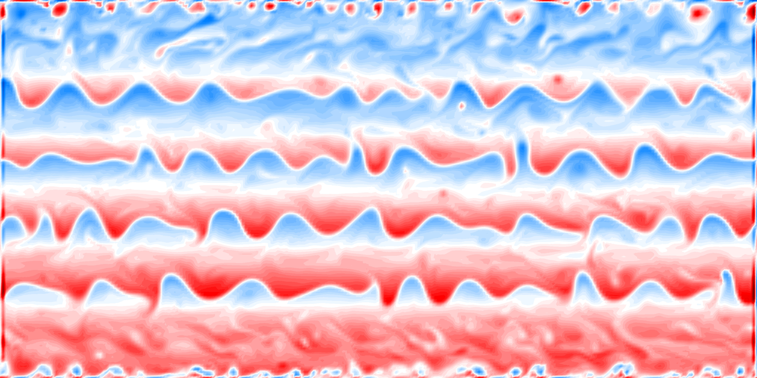
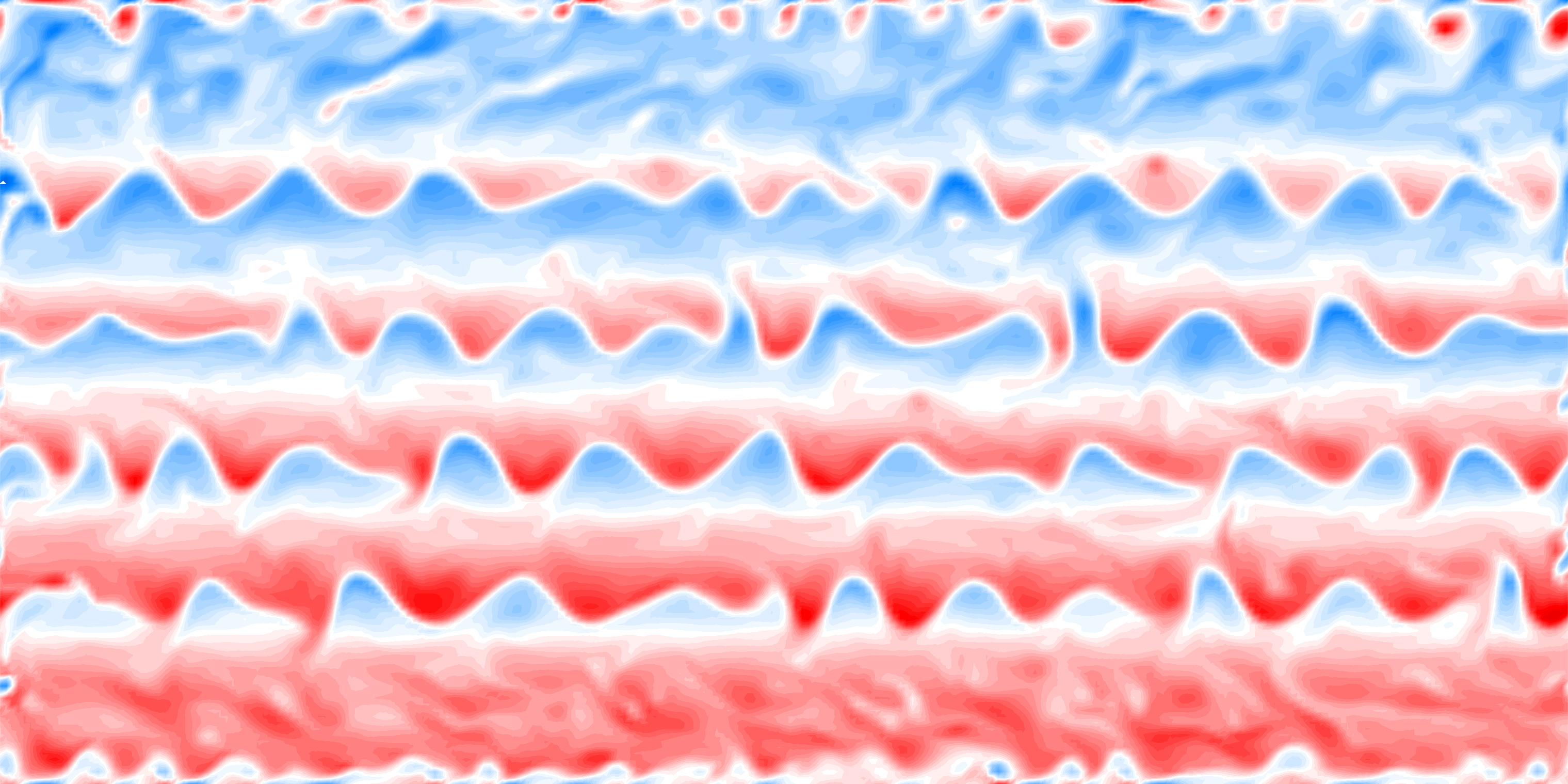
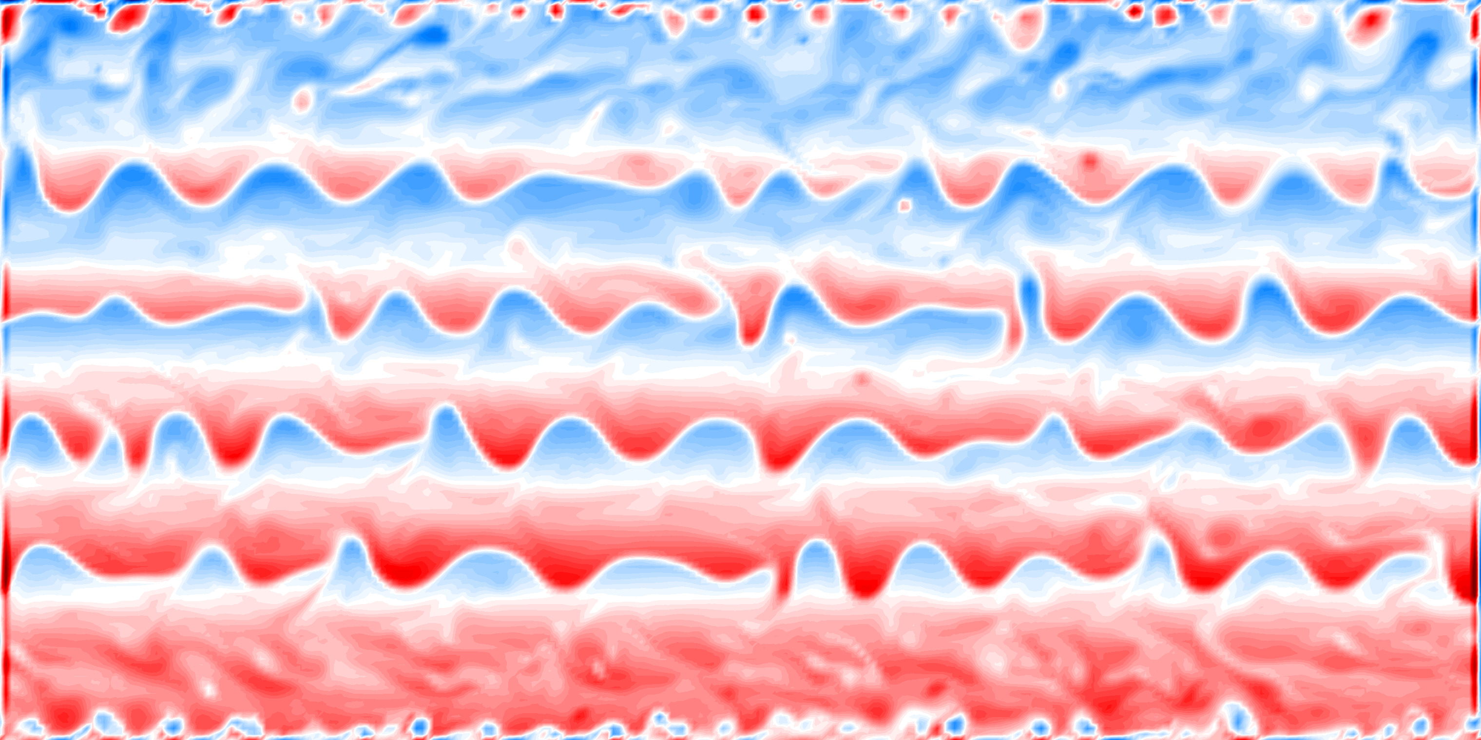
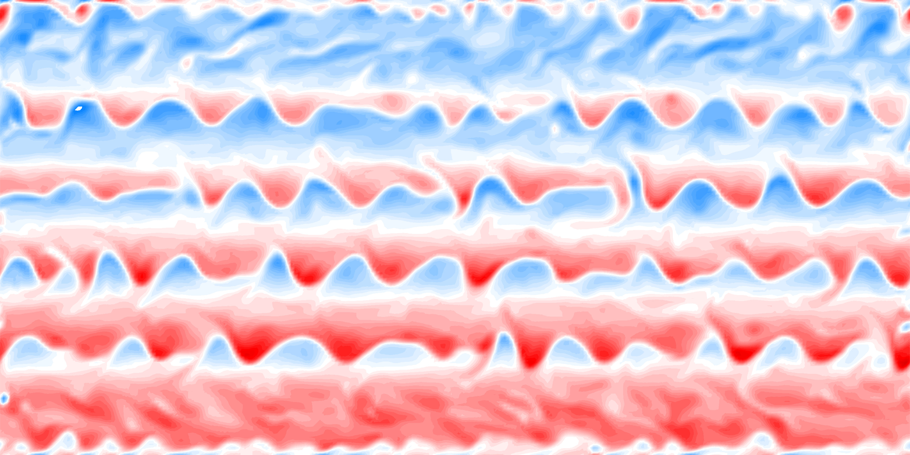
Finally, we have compared true PV anomaly $q$ fields and the ones computed with using the data assimilation methodology based on tempering, jittering, and nudging (Algorithm 5), see Fig. 19.

	$q^{a}_{1}$	$\bar{q}^{p}_{1}$
$t=1$ day
$t=10$ days
$t=20$ days

Figure 19: The series of snapshots shows the true deterministic solution $q^{a}_{1}$ and parameterised solution $\bar{q}^{p}_{1}$ (averaged over the stochastic ensemble of size $N=100$) computed with the data assimilation Algorithm 5. All the solutions were computed on the same coarse grid $G^{c}=257\times 129$, have the same initial condition, and the parameterised solution uses 32 leading EOFs, and 32 weather stations. All the fields are given in units of $[s^{-1}f^{-1}_{0}]$, where $f_{0}=0.83\times 10^{-4}\,{\rm s^{-1}}$ is the Coriolis parameter.

As Fig. 19 shows, the paramaterised solution $\bar{q}^{p}_{1}$ using the data assimilation methodology based on tempering, jittering, and nudging (Algorithm 5) gives an accurate forecast of the true state $q^{a}_{1}$ even with a very small number of weather stations.

7 Conclusion and future work

In this paper, we have reported on our recent progress in developing an ensemble based data assimilation methodology for high dimensional fluid dynamics models. Our methodology involves a particle filter which combines model reduction, tempering, jittering, and nudging. The methodology has been tested on the two-layer quasi-geostrophic model with $O(10^{6})$ degrees of freedom. Only a minute fraction of these are noisily observed (16 and 32 weather stations). The model is reduced by following the stochastic variational approach for geophysical fluid dynamics introduced in holm2015variational . We have also introduced a stochastic time-stepping scheme for the quasi-geostrophic model and have proved its consistency in time. In addition, we have analyzed the effect of different procedures (tempering, jittering, and nudging) on the accuracy and uncertainty of the stochastic spread. Our main findings are as follows:

• The tempering and jittering procedure (Algorithm 4) improves the accuracy by reducing the uncertainty of the stochastic spread;

• The nudging procedure (Algorithm 5) brings major improvements to the combinations of the tempering and jittering (Algorithm 4), both in terms of the relative bias (RB) and ensemble mean relative $l_{2}$-norm error (EME)

• The number of weather stations has a minor effect on the RB and EME;

• The size of the data assimilation step has a substantial effect; namely, the smaller the data assimilation step, the higher the accuracy;

• The resolution of the signal grid significantly improves the accuracy and reduces the uncertainty of the stochastic spread;

• The proposed data assimilation methodology corrects the bias introduced by the paramaterisation and produces a reliable forecast.

We regard the data assimilation method based on tempering and jittering combined with the nudging method proposed here as a potentially valuable addition to data assimilation methodologies. We also expect it to be useful in developing data assimilation methodologies for larger, more comprehensive ocean models. The combination of the four components presented here (model reduction, tempering, jittering and nudging) can be enhanced by further improvements including localization, space-time data assimilation, etc. Applications of these combined components will form the subject of subsequent work.

Conflict of interest

The authors declare that they have no conflict of interest.

References

- [1] J. Anderson. A method for producing and evaluating probabilistic forecasts from ensemble model integrations. J. Climate, 9:1518–1530, 1996.
- [2] A. Arakawa. Computational design for long-term numerical integration of the equations of fluid motion: two-dimensional incompressible flow. Part I. J. Comput. Phys., 1:119–143, 1966.
- [3] P. Berloff and I. Kamenkovich. On spectral analysis of mesoscale eddies. Part I: Linear analysis. J. Phys. Oceanogr., 43:2505–2527, 2013.
- [4] A. Beskos, D. Crisan, and A. Jasra. On the stability of sequential Monte Carlo methods in high dimensions. Ann. Appl. Prob., 24:1396–1445, 2014.
- [5] C. Cotter, D. Crisan, D. Holm, W. Pan, and I. Shevchenko. Modelling uncertainty using circulation-preserving stochastic transport noise in a 2-layer quasi-geostrophic model. arXiv:1802.05711 [physics.flu-dyn], 2018.
- [6] C. Cotter, D. Crisan, D. Holm, W. Pan, and I. Shevchenko. A Particle Filter for Stochastic Advection by Lie Transport (SALT): A case study for the damped and forced incompressible 2D Euler equation. arXiv:1907.11884 [stat.AP], 2019.
- [7] C. Cotter, D. Crisan, D. Holm, W. Pan, and I. Shevchenko. Numerically modelling stochastic Lie transport in fluid dynamics. Multiscale Model. Simul., 17:192–232, 2019.
- [8] D. Crisan and A. Doucet. A survey of convergence results on particle filtering methods for practitioners. IEEE Trans. Signal Processing, 50:736–746, 2002.
- [9] A. Doucet, N. Freitas, and N. Gordon. Sequential Monte Carlo Methods in Practice. Springer, 2001.
- [10] A. Farhat, R. L. Panetta, E. S. Titi, and M. Ziane. Long-time behavior of a two-layer model of baroclinic quasi-geostrophic turbulence. J. Math. Phys., 53:1–24, 2012.
- [11] D. Holm. Variational principles for stochastic fluids. Proc. Roy. Soc. A, 471, 2015.
- [12] W. Hundsdorfer, B. Koren, M. van Loon, and J. Verwer. A positive finite-difference advection scheme. J. Comput. Phys., 117:35–46, 1995.
- [13] S. Karabasov, P. Berloff, and V. Goloviznin. CABARET in the ocean gyres. Ocean Model., 2–3:155–168, 2009.
- [14] P. Kloeden and E. Platen. Numerical solution of stochastic differential equations. Springer-Verlag, Berlin Heidelberg, 1999.
- [15] J. McWilliams. A note on a consistent quasigeostrophic model in a multiply connected domain. Dynam. Atmos. Ocean, 5:427–441, 1977.
- [16] J. Pedlosky. Geophysical fluid dynamics. Springer-Verlag, New York, 1987.
- [17] R. Potthast, A. Walter, and A. Rhodin. A Localized Adaptive Particle Filter within an Operational NWP Framework. Monthly Weather Review, 147:345–362, 2019.
- [18] I. Shevchenko and P. Berloff. Multi-layer quasi-geostrophic ocean dynamics in eddy-resolving regimes. Ocean Modell., 94:1–14, 2015.
- [19] I. Shevchenko and P. Berloff. Eddy backscatter and counter-rotating gyre anomalies of midlatitude ocean dynamics. Fluids, 1:1–16, 2016.
- [20] C. Shu and S. Osher. Efficient implementation of essentially non-oscillatory shock-capturing schemes. J. Comput. Phys., 77:439–471, 1988.
- [21] G. Vallis. Atmospheric and oceanic fluid dynamics: Fundamentals and large-scale circulation. Cambridge University Press, Cambridge, UK, 2006.
- [22] van P. Leeuwen, H. Künsch, L. Nerger, R. Potthast, and S. Reich. Particle filters for high-dimensional geoscience applications: A review. Quarterly J. Royal Meteorlog. Soc., pages 1–31, 2019.
- [23] P. Woodward and P. Colella. The numerical simulation of two-dimensional fluid flow with strong shocks. J. Comput. Phys., 54:115–173, 1984.