Observing the tail of reionization: neutral islands in the $z=5.5$ Lyman-$\alpha$ Forest

Abstract

Previous studies have noted difficulties in modeling the highest opacities of the $z>5.5$ Ly$\alpha$ forest, epitomized by the extreme Ly$\alpha$ trough observed towards quasar ULAS J0148+0600. One possibility is that the most opaque regions at these redshifts contain significant amounts of neutral hydrogen. This explanation, which abandons the common assumption that reionization ended before $z=6$, also reconciles evidence from independent observations of a significantly neutral Universe at $z=7.5$. Here we explore a model in which the neutral fraction is still $\approx 10\%$ at $z=5.5$. We confirm that this model can account for the observed scatter in Ly$\alpha$ forest opacities, as well as the observed Ly$\beta$ transmission in the J0148 trough. We contrast the model with a competing “earlier" reionization scenario characterized by a short mean free path and large fluctuations in the post-reionization ionizing background. We consider Ly$\alpha$ and Ly$\beta$ effective optical depths, their correlations, trough size distributions, dark pixel fractions, the IGM thermal history, and spatial distributions of Lyman-$\alpha$ emitters around forest sight lines. We find that the models are broadly similar in almost all of these statistics, suggesting that it may be difficult to distinguish between them definitively. We argue that improved constraints on the mean free path and the thermal history at $z>5$ could go a long way towards diagnosing the origin of the $z>5.5$ opacity fluctuations.

1 Introduction

Constraints on the timing and duration of reionization provide insight into the first sources of ionizing photons in the Universe. The modern view is that the bulk of reionization occurred between $z\approx 6-10$. This is based largely on the Thomson scattering optical depth ($\tau_{\rm es}$) constraints from the Planck satellite, which place the mid-point of reionization at $z_{\rm re}\simeq 7.7\pm 0.7$ (Planck Collaboration et al., 2018). Further evidence comes from the rapidly declining number density of Ly$\rm{\alpha}$ emitters (LAEs) at $z>6$ (e.g. Schenker et al., 2012; Schmidt et al., 2016; Mason et al., 2018), as well as damping wing features and small proximity zones in the spectra of the highest redshift quasars (Mortlock et al., 2011; Bañados et al., 2018; Davies et al., 2018b). On the other hand, a common working assumption, based on the prevalence of Ly$\alpha$ forest transmission, is that reionization was complete before $z=6$ (Songaila, 2004; Fan et al., 2006; McGreer et al., 2015). Here we will consider the possibility that reionization ended significantly later than $z=6$.

More potential evidence for late reionization comes from large opacity fluctuations in the $z>5$ Ly$\rm{\alpha}$ forest. A sharp increase in the overall opacity, and in its scatter on $50h^{-1}$ Mpc scales, was observed in Fan et al. (2006), and later confirmed by others (Becker et al., 2015; Bosman et al., 2018; Eilers et al., 2018). While the rapid evolution in the overall opacity is not by itself an unambiguous signature of reionization (McQuinn et al., 2011), the scatter is harder to explain otherwise (for some attempts, see D’Aloisio et al., 2015; Davies & Furlanetto, 2016; Chardin et al., 2017).

Of particular importance is the $110h^{-1}$ Mpc long Ly$\rm{\alpha}$ trough centered at $z\approx 5.7$ in the sightline of quasar ULAS J0148+0600 (henceforth J0148; Becker et al. 2015). Interestingly, the trough exhibits significant transmission in the coeval Ly$\beta$ forest, which seemed to reaffirm that reionization ended by $z=6$. A key insight came when the test of Davies et al. (2018a) was carried out by Becker et al. (2018). They measured the spatial distribution of $z=5.7$ LAEs centered on the J0148 trough, probing the large-scale density of the region. The observed deficit of LAEs within $20h^{-1}$ Mpc of J0148 suggests that the sightline passes through a cosmic void. This interpretation is supported by a deficit of Lyman Break Galaxies around the sight line (Kashino et al., 2019).

The prevailing model after Becker et al. (2018) was that of Davies & Furlanetto (2016), in which in which the opacity variations are driven by large fluctuations in the post-reionization ultraviolet background (UVB). The measurements of Becker et al. (2018), however, also raised interesting questions in the context of late reionization. If reionization ended around $z=6$, then the J0148 void was likely reionized not much earlier than $z=6$. In this case, the void should have been hot ($T\sim 20,000$ K), which would make more extreme the low level of UVB needed to reproduce the Ly$\alpha$ trough, because the amount of absorbing H$\,\rm\scriptstyle I\$scales as $T^{-0.7}$ (D’Aloisio et al., 2015, 2019). Also, lowering the mean free path significantly, as is required in the model of Davies & Furlanetto 2016, increases proportionately the ionizing emissivity that is needed to complete reionization (D’Aloisio et al., 2018), perhaps requiring larger escape fractions.

An alternative model explored in Kulkarni et al. (2019) and Keating et al. (2019) circumvents these issues by abandoning the assumption that reionization ended by $z=6$. In their model, reionization ends at $z\approx 5.2$ such that the voids still contain significant amounts of neutral hydrogen at $z>5.5$. The “neutral islands" are the essential new ingredient for reproducing the high opacity tail of the Ly$\alpha$ forest fluctuations. Notably, this model is consistent with evidence of a significantly neutral IGM at $z=7.5$, and it naturally produces long Ly$\rm{\alpha}$ troughs like the one in J0148 (Keating et al., 2019). If confirmed, the model places reionization squarely in the regime where its tail end could potentially be studied directly with existing Ly$\rm{\alpha}$ and Ly$\beta$ forest spectra.

In this paper we further study the scenario in which reionization was still ongoing at $z=5.5$. In contrast to the radiative transfer simulations of Kulkarni et al. (2019) and Keating et al. (2019), we employ approximate “semi-numeric" methods to model reionization’s effects on the forest. We will exploit the flexibility and inexpensiveness of these methods to explore the parameter space of reionization, adding to the previous studies. A basic question that we aim to address here is as follows. Consider two scenarios that both reproduce the large scatter in the $z>5$ forest. In one scenario, the scatter is driven by neutral islands from ongoing reionization (Kulkarni et al., 2019; Keating et al., 2019). In the other, it is driven by large UVB fluctuations in the post-reionization IGM (Davies & Furlanetto, 2016; D’Aloisio et al., 2018). Can we easily distinguish between these scenario with existing data?

The remainder of this paper is organized as follows. In §2, we describe the simulations and modeling methods used in this work. In §3, we present our reionization models and provide physical insight into their features, including the existence of long Ly$\alpha$ troughs. In §4, we explore statistical tests to distinguish between the models. Lastly, we summarize our results in §5. Throughout this paper we use comoving distances unless otherwise stated. We adopt cosmological parameters of $\Omega_{\rm m}=0.31$, $\Omega_{\rm\Lambda}=0.692$, $h=0.68$, $\Omega_{\rm b}=0.048$, $\sigma_{\rm 8}=0.82$ and $n=0.97$ consistent with the Planck measurements (Planck Collaboration et al., 2018).

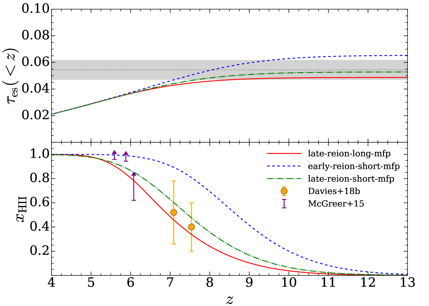
Figure 1: Reionization histories of the models used in this work. Top: the integrated electron scattering optical depth parameter, $\tau_{\rm es}$. The grey shading spans the $1\sigma$ limits from Planck Collaboration et al. (2018). Bottom: The redshift evolution of the volume-weighted average H$\,\rm\scriptstyle I\$ fraction. For reference, we show constraints from the dark pixel analysis of McGreer et al. (2015) and the damping wing analysis of Davies et al. (2018b) using high-$z$ quasars at $z\simeq 7.1$ and $7.5$.

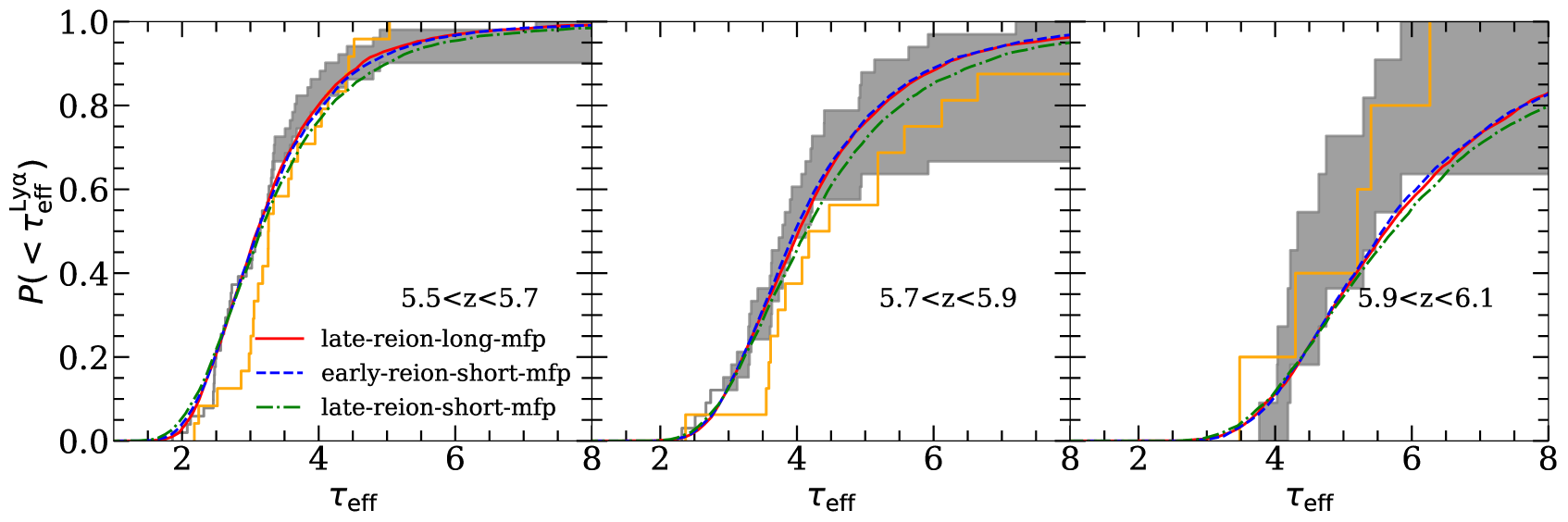
Figure 2: Comparison of the Ly$\alpha$ forest effective optical depth ($\tau_{\rm{eff}}\,$) distributions in our models. The grey histograms show the measurements of Bosman et al. (2018). The shading spans their “optimistic" and “realistic" treatments of non-detections. The orange histograms show the measurements of Eilers et al. (2018). Note that we have calibrated our models to match the mean fluxes reported by Bosman et al. (2018).

2 Numerical Methodology

We post-process a cosmological hydrodynamics simulation to model large-scale fluctuations in the Ly$\rm{\alpha}$ forest. Here we describe the elements of our numerical modeling. Readers uninterested in these technical details may skip to §3 without loss of continuity.

2.1 Hydrodynamics simulation

The basis of our models is an Eulerian hydrodynamics simulation that we ran with a modified version of the code of Trac & Pen (2004). The run has $2\times 2048^{3}$ gas and dark matter resolution elements in a box with $L=200$ $h^{-1}{\rm Mpc}\,$. The simulation was initialized at $z=300$ using first-order Lagrangian perturbation theory and transfer functions generated by CAMB (Lewis et al., 2000). The gas was nominally flash ionized to a temperature of 20,000 K at $z=7.5$ and a uniform ionizing background with $J_{\rm\nu}\propto\nu^{-1.5}$ between 1 and 4 Ry was applied thereafter (here $\nu$ is frequency). The strength of the background is tuned such that the hydrogen photoionization rate is $\Gamma_{\mathrm{HI}}=10^{-13}\mathrm{s}^{-1}$, but in the ensuing sections we will describe how we post-process the simulation to model fluctuations in $\Gamma_{\mathrm{HI}}$, as well as in the gas temperature. The hydro simulation setup is nearly identical to that in D’Aloisio et al. (2018).

2.2 Semi-numerical reionization simulation

We apply the excursion set model of reionization (ESMR) (Furlanetto et al., 2004; Mesinger et al., 2011) to obtain realizations of the reionization redshift field, $z_{\rm{re}}\,$$(\mathbf{x})$. We filter the initial density field of our hydro simulation on a hierarchy of scales and compute the local collapsed fraction using the conditional Press-Schechter expression, $f_{\rm coll}=\mathrm{erfc}\left[(\delta_{c}(z)-\delta_{m})/\sqrt{2(\sigma^{2}(m_{\mathrm{min}})-\sigma^{2}(m))}\right]$, where $\delta_{c}(z)$ is the critical density in the spherical collapse model, $\delta_{m}$ is the mean linear density contrast within a spherical top-hat containing mass $m$, and $\sigma^{2}(m)$ is the variance of linear density fluctuations on scale $m$ (Press & Schechter, 1974; Bond et al., 1991; Lacey & Cole, 1994). We flag a cell as ionized once the condition $\zeta f_{\rm coll}\geq 1$ is met, where $\zeta$ is a constant ionizing efficiency parameter that encapsulates the efficiency at which collapsed baryons form stars and deliver ionizing photons to the IGM. The minimum halo mass for forming galaxies is assumed to be $m_{\mathrm{min}}=2\times 10^{9}$ $M\textsubscript{$\odot$}$, and we tune $\zeta$ to achieve the desired reionization histories (see §3). The mean free path is modeled in a simplistic way by adopting the maximum filter scale as a free parameter (Furlanetto & Oh, 2005; Mesinger et al., 2011). We find that imposing a mean free path in the ESMR, albeit crudely, is required to produce reasonable ionization front (I-front) speeds ($\lesssim 10^{4}$ km/s) toward the end of reionization (see D’Aloisio et al., 2019; Deparis et al., 2019). Our reionization models are generated on a coarser grid of size $N=256^{3}$, with a spatial resolution of $\Delta x=0.78$ $h^{-1}{\rm Mpc}\,$. This is sufficient for our purposes given that the approach used here is unlikely to capture the detailed structure of reionization on scales $\lesssim 1$ $h^{-1}{\rm Mpc}\,$.

2.3 Temperature fluctuations from reionization

To model the imprint of reionization on IGM temperatures, we adopt an approach similar to that of D’Aloisio et al. (2019) (see also Upton Sanderbeck et al. 2016; Davies et al. 2018a). The temperature evolution of each gas parcel with over-density, $\Delta$, after it has been reionized, is governed by (e.g. Miralda-Escudé & Rees, 1994; McQuinn & Upton Sanderbeck, 2016)

$$\frac{dT}{dt}=\frac{2\mu m_{H}}{3k_{B}\rho}(\mathscr{H}-\Lambda)+\frac{2T}{3\Delta}\frac{d\Delta}{dt}-2HT,$$ (1)

where $H$ is the Hubble parameter, $\mathscr{H}$ is the sum of the photo-heating rates, and $\Lambda$ contains the radiative cooling rates. The second term on the right describes adiabatic heating and cooling from structure formation. The final term arises from adiabatic cooling due to the expansion of the Universe. Strictly speaking, equation (1) applies in the Lagrangian picture but we use it here to describe the temperature evolution of our Eulerian gas cells. We aim to model the large-scale structure of the temperature field during/after reionization, and not the details on small scales. D’Aloisio et al. (2019) found that the above approximation works well for this purpose when compared against a fully coupled radiative hydrodynamics simulation.

For each of our reionization models, we use the $z_{\rm{re}}\,$ field to compute the I-front velocity field, $v_{\rm IF}$, for each cell using the gradient method of D’Aloisio et al. (2019) (see also Deparis et al. 2019). Each cell is then initialized to a post-I-front temperature, $\,T_{\rm reion}\,$$(v_{\rm IF})$, at the appropriate $z_{\rm{re}}\,$ using the fitting formula of D’Aloisio et al. (2019). The subsequent evolution is obtained by solving the Eq. (1) numerically assuming a post-reionization ionizing background with $J_{\nu}\propto\nu^{-1.5}$ between 1 and 4 Ry. McQuinn & Upton Sanderbeck (2016) showed that the temperature evolution in the diffuse IGM is relatively insensitive to the evolution of $\Delta$ under realistic assumptions. Here we adopt the Zel’dovich pancake approximation to propagate backwards or forward in time the $z=5.8$ density values from our hydro simulation. We adopt a fixed temperature of $T=10K$ for pre-reionization cells, but all of our results pertaining to observable quantities are insensitive to this choice. Our temperature calculations are performed at the resolution of our hydro simulation, but note that the $z_{\rm{re}}\,$fields, and therefore the $\,T_{\rm reion}\,$fields, are at the coarser resolution of $N=256^{3}$.

2.4 UVB fluctuations

Our models also include UVB fluctuations with a version of the Davies & Furlanetto (2016) model, modified to achieve higher resolutions and to approximate the radiative transfer shadowing effects around neutral islands. For late reionization models, we will find that the shadowing is crucial for generating large opacity fluctuations. The basic setup is similar to that in D’Aloisio et al. (2018). Halos were identified using a spherical over-density criterion of 200 times the cosmic mean matter density. We then abundance matched the halos to an interpolation of the rest-frame UV luminosity functions of Bouwens et al. (2015b). We assume that all halos with masses above $2\times 10^{10}~{}h^{-1}M_{\odot}$ (with at least $\approx 300$ dark matter particles) host a star forming galaxy. This limit was chosen for completeness of the halo mass function, i.e. faithfully reproducing the mass function measured from the SCORCH I suite of N-body simulations, which includes runs that extend well beyond our resolution limit (Trac et al., 2015). Note that, owing to the resolution of our hydro simulation, the minimum mass for these calculations is necessarily different than the $M_{\rm min}=2\times 10^{9}$ $M_{\odot}$ used for the ESMR calculations. We do not expect this to change our main conclusions, however, as most of the effects of larger $M_{\rm min}$ could be mimicked by using a somewhat lower mean free path.

To model the spatially varying mean free path, we bin the sources onto a coarse grid with $N=64^{3}$ and iteratively solve for $\Gamma_{\rm HI}(\mathbf{x})$ and $\,\lambda_{\rm mfp}\,$$(\mathbf{x})$ under the assumption that the latter scales as $\,\lambda_{\rm mfp}\,$$\propto{\Gamma}_{\rm HI}^{2/3}/\Delta$. This scaling is motivated by analytic models (Miralda-Escudé et al., 2000; Furlanetto & Oh, 2005) and by the scaling measured in radiative transfer simulations (McQuinn et al., 2011). Our main upgrade to the approach of Davies & Furlanetto (2016) is that we add a second step in which we use the coarse $N=64^{3}$ $\,\lambda_{\rm mfp}\,$ field together with a direct sum over sources to recalculate $\Gamma_{\rm HI}(\mathbf{x})$ on a higher resolution grid with $N=256^{3}$ (the same resolution as our ESMR grids). In this step, we remove ionizing photon contributions from sources whose sight lines pass through neutral islands. We will see that this shadowing by the neutral islands leads to suppressed $\Gamma_{\mathrm{HI}}$ in their vicinity. In what follows, we will characterize our models with $\langle\lambda^{912}_{\rm mfp}\rangle(z)$, the volume-weighted average over our mean free path fields. (Here the “912" denotes 912 Å.) In all of our models, we set the maximum filter scale in our ESMR calculations to $\langle\lambda^{912}_{\rm mfp}\rangle(z=5.6)$ in an attempt to make the reionization models more consistent with the above fluctuating UVB models. Lastly, we note that our approach does not capture the effects of the shadowing on the local mean free path near the neutral islands. In reality, the $\Gamma_{\mathrm{HI}}$ around the islands may be even lower from this effect.

2.5 Synthetic Ly$\alpha$/$\beta$ forest sight lines

Finally, to construct synthetic quasar absorption spectra, we trace $4000$ sight-lines at random angles through the simulation box, each with length of 500$h^{-1}{\rm Mpc}\,$(making use of the periodic boundary conditions). The neutral hydrogen densities for the ionized gas along the skewers are rescaled using our fluctuating temperature and $\Gamma_{\rm HI}$ fields under the assumption of photoionization equilibrium, and we set cells to be fully neutral if $z>z_{\rm re}$ according to the ESMR grids. We calculate Ly$\alpha$ and Ly$\beta$ opacities along the sight lines using the (accurate) approximation of Tepper-García (2006) to the Voigt profile. We iteratively adjust the normalization of $\Gamma_{\mathrm{HI}}$$(\mathbf{x})$ in the ionized regions to match the mean Ly$\alpha$ forest flux with observed values. Unless otherwise noted, we match to the mean fluxes reported by Bosman et al. (2018). For some calculations (e.g. long Ly$\alpha$ troughs), we account for evolution in $\Gamma_{\mathrm{HI}}$ along the skewers by fitting a 4th order polynomial to the normalization of $\Gamma_{\mathrm{HI}}$ between $z=5.5-6$ and rescaling the skewers as a function of redshift. We model instrumental noise by drawing pixel-by-pixel from a Gaussian distribution according to the desired level of signal to noise ($S/N$). Because this parameter depends on the particular comparison with observations, we provide these details below.

Table 1: Summary of models used in this work. The mean free paths are quoted in units of comoving $h^{-1}$Mpc (see text for a definition of these average quantities). The middle three columns give volume-weighted mean H$\,\rm\scriptstyle I\$fractions at select redshifts. The right-most columns give the mean $\Gamma_{\mathrm{HI}}$ in units of $\times 10^{-12}$ s^-1.

Model		$\langle\lambda^{912}_{\rm mfp}\rangle$			$\langle x_{\rm HI}\rangle$			$\langle\Gamma_{-12}\rangle$
	$z=5.6$	$z=5.8$	$z=6.0$	$z=5.6$	$z=5.8$	$z=6.0$	${z=5.6}$	${z=5.8}$	${z=6.0}$
late-reion-long-mfp.	30	27	23	0.097	0.141	0.194	0.39	0.25	0.15
early-reion-short-mfp	10	9	8	0.005	0.009	0.014	0.54	0.33	0.19
late-reion-short-mfp	10	9	8	0.074	0.100	0.133	0.48	0.29	0.17

3 Models of Reionization

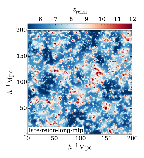
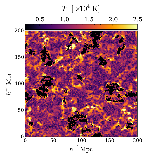
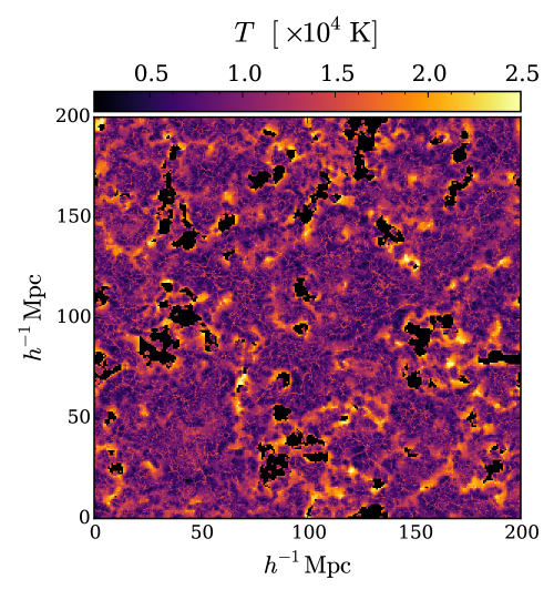
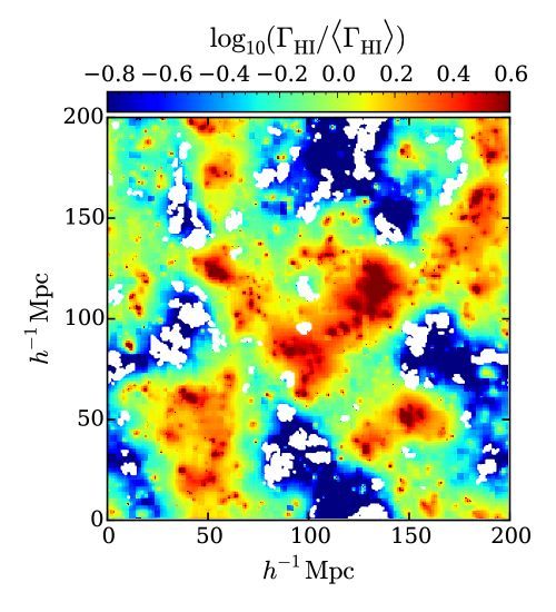
Figure 3: Slices through our simulations at $z=5.6$, showing the interplay between fluctuations in our models. From top row to bottom: late-reion-long-mfp, early-reion-short-mfp and late-reion-short-mfp. The left, middle, and right columns correspond to slices through the reionization redshift field, the temperature field, and the H$\,\rm\scriptstyle I\$ photoionization rate. Neutral islands are shown in black (white) in the middle (right) panels.

3.1 Reionization scenarios

We model three broadly different reionization scenarios to explore whether they might be immediately distinguishable with current observations. Our models are characterized by the timing of reionization’s end and by $\langle\lambda^{912}_{\rm mfp}\rangle(z)$. The mean free path at $z>5$ is highly uncertain and even today’s large-volume radiative transfer simulations of reionization likely lack the resolution to model it accurately. Here we vary $\langle\lambda^{912}_{\rm mfp}\rangle(z)$ by a factor of 3 amongst our models to explore the widely open parameter space.

The reionization histories of our models are shown in the bottom panel Fig. 1. For reference, we also show the $1\sigma$ constraints of McGreer et al. (2015) and Davies et al. (2018b). The top panel shows the corresponding cumulative electron scattering optical depths, $\tau_{\rm es}(<z)$, compared against the 1$\sigma$ limits measured by Planck (Planck Collaboration et al., 2018). Table 1 quantifies the mean free path and timing of reionization in our models. For simplicity, we adopt a redshift dependence of $\lambda^{912}_{\rm mfp}\propto(1+z)^{-4.4}$, in accordance with the fitting formula of Worseck et al. (2014), which captures the trend of measurements at $z\lesssim 5.2$. For reference, extrapolating the fit of Worseck et al. (2014) to higher redshifts yields $\lambda^{912}_{\rm mfp}=38,34$ and $30$ $h^{-1}{\rm Mpc}\,$  at $z=5.6,5.8$ and $6.0$, respectively.

Our fiducial model (red/solid) is a late reionization scenario with a significant amount of neutral hydrogen remaining in the IGM at $z=5.5$, and with a (relatively) longer $\langle\lambda^{912}_{\rm mfp}\rangle$. We will see that large opacity fluctuations are driven by the presence of neutral islands in this model, which we denote as late-reion-long-mfp. We will contrast this scenario against an updated version of the competing model of Davies & Furlanetto (2016), in which reionization ends before $z\simeq 6$ (blue/dashed curves in Fig. 1). The defining feature is that $\langle\lambda^{912}_{\rm mfp}\rangle$ is a factor of 3 shorter than our fiducial model, resulting in large spatial variations in $\Gamma_{\rm HI}$ that are driven by galaxy clustering (and not neutral islands). The original Davies & Furlanetto (2016) model did not include the effects of temperature fluctuations from reionization, which amounted to an implicit assumption that reionization ended early enough for the temperature-density relation to have relaxed to a tight power-law form (Hui & Gnedin, 1997; McQuinn & Upton Sanderbeck, 2016). Here we update the model by adding in temperature fluctuations consistent with reionization ending at $z\approx 6$. We will denote this model with early-reion-short-mfp. Lastly, we constructed a late-reion-short-mfp model that blends the two scenarios. In this model (green/dot-dashed), the global neutral fractions are similar to our fiducial model at $z<6$, but $\langle\lambda^{912}_{\rm mfp}\rangle$ is a factor of 3 shorter. Hence there are large $\Gamma_{\mathrm{HI}}$ fluctuations from both the short mean free path and the neutral islands.

The right three columns of Table 1 show the mean values of $\Gamma_{\mathrm{HI}}$ in our models after matching mean fluxes to the observed values of Bosman et al. (2018). We have applied the correction factors in the appendix of D’Aloisio et al. (2018) in order to correct for finite resolution. These values are reasonably consistent with the measurements of D’Aloisio et al. (2018) given differences in the thermal histories of our simulations and in the mean fluxes measured by Bosman et al. (2018) and Becker et al. (2015).

In Fig. 2 we compare our model distributions of $\tau_{\rm{eff}}\,$ against the measurements of Bosman et al. (2018) (gray shading) as well as the measurements of Eilers et al. (2018) (orange) in 3 redshift bins. Unless otherwise noted, we define $\tau_{\rm{eff}}\,$ in terms of an average of the continuum normalized flux, $F$, over 50$h^{-1}$ Mpc segments, $\tau_{\rm{eff}}\,$$=-\ln\langle F\rangle$. The shading spans the “optimistic" and “pessimistic" treatments of the non-detections in Bosman et al. (2018). The former takes the $2\sigma$ upper limits on the fluxes for measurements and the latter assigns zero flux.

3.2 Deconstructing the Ly$\rm{\alpha}$ forest fluctuations

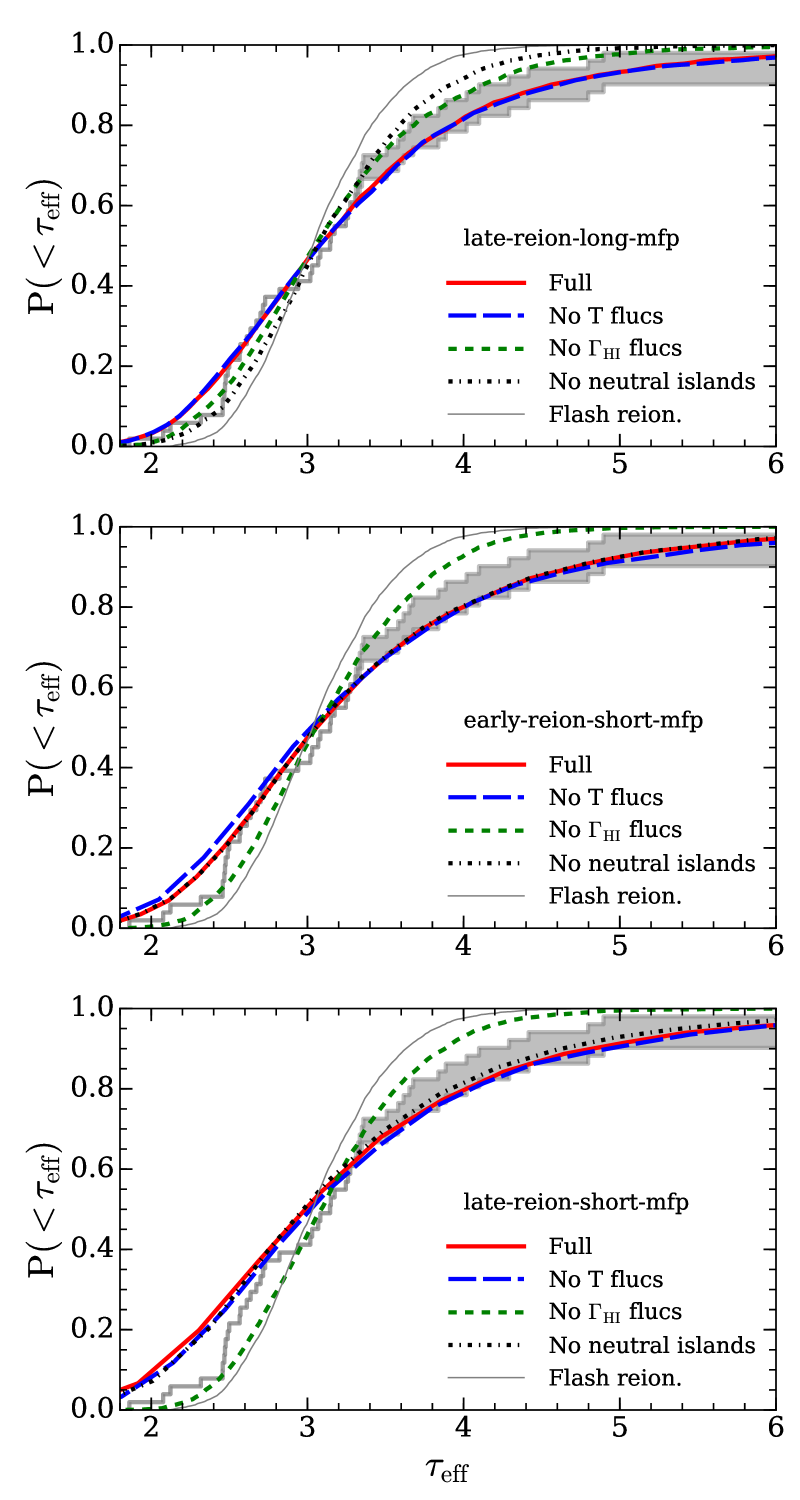
Figure 4: Deconstructing our models of the Ly$\rm{\alpha}$ forest opacity fluctuations. Here we show a series of tests in which we leave out, one by one, the sources of fluctuation in our models. “No T flucs" denotes leaving out the temperature fluctuations from reionization, “No $\Gamma_{\rm HI}$ flucs" denotes setting $\Gamma_{\rm HI}$ to a uniform value (outside of neutral regions). Lastly, “No neutral islands" denotes removing the neutral islands, including their shadowing effects on the UVB. Here we consider the distributions of $\tau_{\rm{eff}}\,$ at $z=5.6$. These results show that, in the late-reion-long-mfp model, the opacity fluctuations are driven by neutral islands and their shadowing effects.

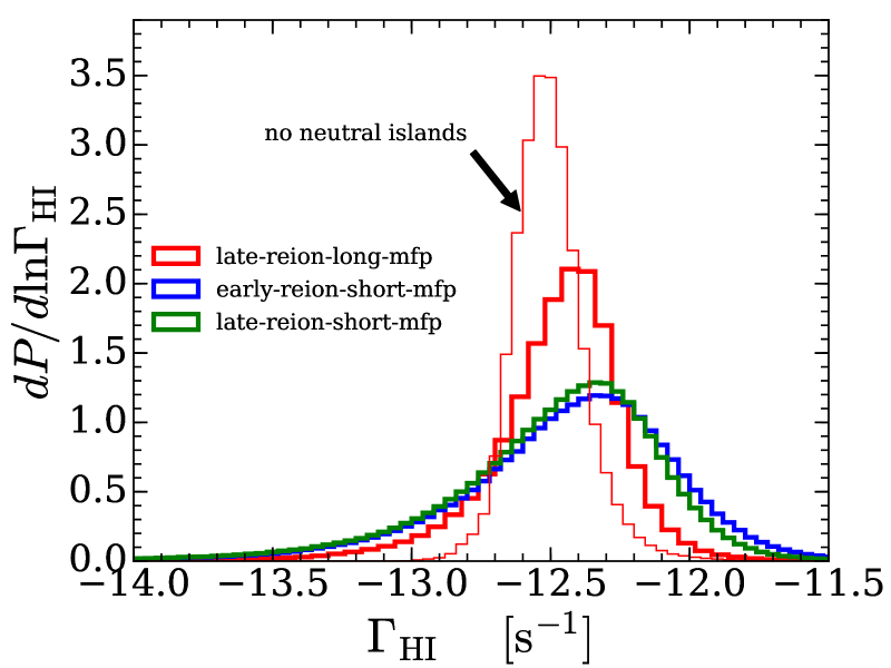
Figure 5: The probability distributions of $\Gamma_{\rm HI}$ in our models at $z=5.6$. The thin red curve shows a variation of the late-reion-long-mfp model in which we leave out the neutral islands. In this model, shadowing of the UVB by the neutral islands creates a low-$\Gamma_{\rm HI}$ tail associated with the highest Ly$\alpha$ forest opacities.

One advantage of our piecemeal modeling is that we can straightforwardly explore the sources of $\tau_{\rm{eff}}\,$ fluctuation by simply leaving them out of the models. In this section we deconstruct the opacity fluctuations to gain physical insight into their origin.

We begin by visualizing the interplay between fluctuations. Fig. 3 shows slices through the reionization redshift (left column), temperature (middle), and H$\,\rm\scriptstyle I\$ photionization rate (right) fields at $z=5.6$. The top, middle, and bottom rows correspond to the late-reion-long-mfp, early-reion-short-mfp, and late-reion-short-mfp models, respectively. In both of the late scenarios there are large pockets of neutral hydrogen, tens of Mpc across, which can be seen as the black (white) regions in the temperature (photoionization rate) panels. Note that the recently reionized gas adjacent to these pockets (closer to the I-fronts) is hotter than the gas elsewhere reionized long ago. The temperature field is more uniform in the early-reion-short-mfp model because the fluctuations have had more time to fade away. Despite the bulk of reionization completing by $z=6$ in this model, there are still tiny neutral islands remaining because the short mean free path creates an extended tail of percent-level neutral fraction. All three models exhibit large fluctuations in the UVB. To gauge the impact of the neutral islands on the UVB, the top-right panel of Fig. 3 may be compared against the top-right panel of Fig. 2 in D’Aloisio et al. (2018). The latter shows what the UVB looks like with $\langle\lambda^{912}_{\rm mfp}\rangle=30h^{-1}$ Mpc, but in the absence of neutral islands.

Figure 4 shows the results of a series of tests where we leave out, one by one, the sources of fluctuation. The curves labeled “full" show the complete models. The curves labeled “no $T$ flucs" correspond to neglecting the temperature fluctuations from reionization (we use the original temperatures from our hydro simulation, which exhibit a tight temperature-density relation). Likewise, the curves labelled “No $\Gamma_{\mathrm{HI}}$ flucs" correspond to adopting the nominal uniform $\Gamma_{\mathrm{HI}}$ of the hydro simulation everywhere outside of the neutral islands (within which $\Gamma_{\mathrm{HI}}$$=0$). For the curves labeled “No neutral islands," we remove the neutral islands as well as their shadowing effects on the UVB. Lastly, the curves labeled “Flash reion." correspond to an instantaneous reionization at $z=7.5$. Here we focus on the $z=5.6$ bin.

Consider first late-reion-long-mfp, shown in the top panel of Fig. 4. Comparing the blue/long-dashed curve to the red/solid curve, we find that removing the temperature fluctuations has no noticeable impact on the width of the $\tau_{\rm{eff}}\,$ distribution. In fact, this is true in all three models because the duration of reionization is too short to generate temperature fluctuations large enough to “win" against the opposing effects of the $\Gamma_{\mathrm{HI}}$ fluctuations, at least when it comes to the $\tau_{\rm{eff}}\,$ fluctuations (see D’Aloisio et al. 2015 for a discussion on the role of reionization’s duration in this context). However, when they are present, we find that the temperature fluctuations do play a significant role in the statistics of the opacities, particularly in generating some of the most transmissive sight lines. We will see one consequence of this in §4.3. Foreshadowing, it appears that the interplay between temperature, $\Gamma_{\mathrm{HI}}$, and neutral islands is non-trivial in these models. We caution that no apparent effect on the $\tau_{\rm{eff}}\,$ distribution should not be interpreted as no effect at all.

The green/short-dashed curve shows that setting $\Gamma_{\rm HI}$ to a uniform value outside of the neutral islands reduces the width and eliminates the high-opacity tail of the $\tau_{\rm{eff}}\,$ distribution. We get a similar (but larger) effect if we instead remove the neutral islands entirely, which includes removing their shadowing effects on the UVB, as illustrated by the black/dot-dashed curve. We find that the difference between the “Full" and “No $\Gamma_{\mathrm{HI}}$ flucs" models owes to the shadowing of the UVB in the vicinity of the neutral islands (which is lacking in the latter). We conclude that both the neutral islands and their shadowing effects are critical for generating the high-opacity tail of the $\tau_{\rm{eff}}\,$ distribution in this model. Note also that the “No neutral island" distribution is wider than the “Flash reion." distribution. We find that this additional width owes to the temperature fluctuations from reionization.

The situation is markedly different for the early-reion-short-mfp model (middle panel). There is no noticeable difference in the $\tau_{\rm{eff}}\,$ distribution when we remove the neutral islands, as expected given the $0.5\%$ global neutral fraction at $z=5.6$. In this model, the high-opacity tail is driven by large $\Gamma_{\rm HI}$ fluctuations whose origin lie in a short $\langle\lambda^{912}_{\rm mfp}\rangle$. Lastly, we consider the late-reion-short-mfp model (bottom panel), which has a similar global neutral fraction to the late-reion-long-mfp model. Interestingly, removing the effects of neutral islands from this model has a relatively mild effect on the distribution. The $\Gamma_{\mathrm{HI}}$ fluctuations are characteristically different between the late-reion-long-mfp and late-reion-short-mfp models because of the different values of $\langle\lambda^{912}_{\rm mfp}\rangle$.

These ideas are further elucidated in the top panel of Figure 5, which compares the probability distributions of $\Gamma_{\mathrm{HI}}$ in our three models. Note the wide range of $\Gamma_{\mathrm{HI}}$ that results from the short $\langle\lambda^{912}_{\rm mfp}\rangle$ in the early-reion-short-mfp model (blue). This is similar to what is seen in the late-reion-short-mfp model (green). The distribution has a different shape in the late-reion-long-mfp model (red). The fluctuations are somewhat smaller, but there is a low-$\Gamma_{\mathrm{HI}}$ tail associated with the most opaque regions of the forest. For reference, the thin red curve shows the distribution when we remove the shadowing effects of the neutral islands in that model. The low-$\Gamma_{\mathrm{HI}}$ tail disappears, illustrating the importance of the shadowing for generating extended low-opacity regions.

3.3 Long Ly$\rm{\alpha}$ Troughs

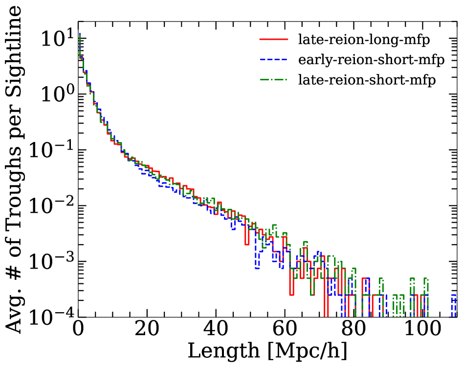
Figure 6: The $5.5<z<5.9$ Ly$\rm{\alpha}$  trough size distributions in our models. Here we show the average number of troughs of a given size per sight line. Note that this quantity yields the frequency of troughs when the average number is much less than unity. The simulated sight lines are processed with ${\rm S/N}=150$ per pixel.

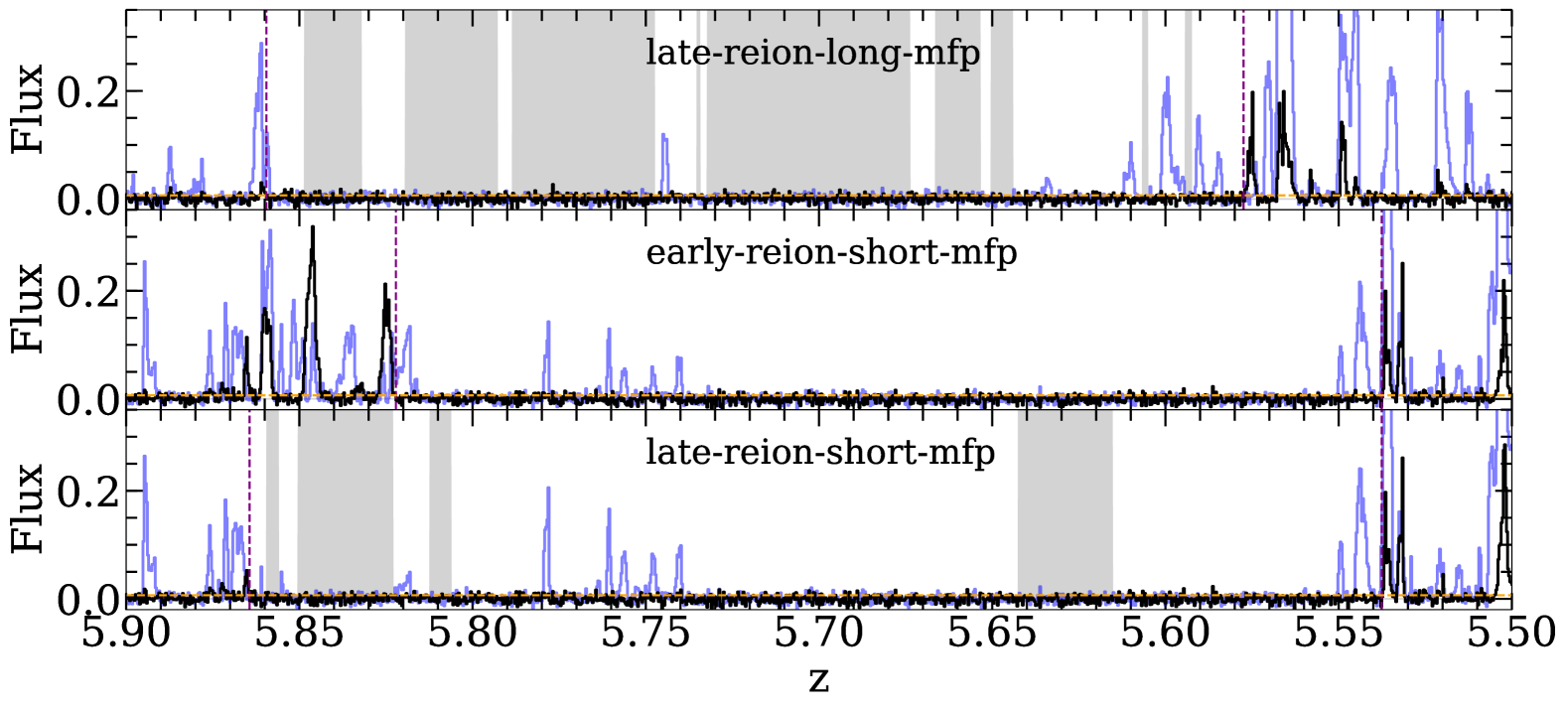
Figure 7: Examples of long Ly$\alpha$ troughs with lengths and Ly$\beta$ opacities similar to those of the J0148 trough observed by Becker et al. (2015). Ly$\alpha$ and Ly$\beta$ transmission are shown in black and blue, respectively. Vertical dashed lines mark the extents of the Ly$\alpha$ troughs. From top to bottom, troughs lengths are 100, 109, 101$h^{-1}{\rm Mpc}\,$ respectively. The Ly$\beta$ $\tau_{\rm{eff}}\,$ are 5.213, 5.137, and 5.152. In all of our models, the most extreme Ly$\alpha$ troughs occur in cosmological voids. Only in the late-reion-long-mfp model are the neutral islands physically necessary for creating the troughs. We note that the most extreme troughs originate from different sight lines in different models. As a result, each example depicts a different sight line (with different density structure).

In this section we examine whether our models reproduce long Ly$\alpha$ troughs like the one observed in J0148. We focus on the redshift range $5.5<z<5.9$ spanned by the J0148 trough. Because of the steep evolution in $\Gamma_{\mathrm{HI}}$ over this interval (D’Aloisio et al., 2018), we include redshift evolution in the manner described in §2.5. We also add noise with ${\rm S/N}=150$ per pixel, approximately matching the noise characteristics of the J0148 spectrum in Becker et al. (2015). We identify Ly$\rm{\alpha}$ troughs as regions between “peaks" where the continuum normalized flux is above 2$\sigma$ of noise at four consecutive pixels (Becker et al., 2015; Keating et al., 2019).

In Fig. 6, we show the Ly$\rm{\alpha}$ trough size distribution extracted at $5.5<z<5.9$. Despite the physical differences between models noted in §3.2, the distributions are very similar, with the longest troughs extending to $\approx 110h^{-1}$ Mpc, similar to the length of the J0148 trough. The incidence of $\sim 100$ Mpc troughs, however, is quite low, occurring in $1-2$ out of 4000 sight lines in all three models. These rates are much lower than the roughly $\gtrsim 1/100$ rate inferred from the existence of J0148, but we note that this discrepancy likely owes to our small box size of $L=200h^{-1}$ Mpc. Capturing the incidence rates of these long troughs requires much larger volumes.

In Fig. 7, we show one example trough from each model, selected with similar characteristics to the J0148 trough. We note that the most extreme troughs originate from different sight lines in different models. As a result, each example depicts a different sight line (with different density structure). The length of these troughs are $\gtrsim 100h^{-1}$ Mpc and they are more dark ($\tau_{\rm{eff}}\,$$>7.7$) than in J0148. One of the defining features of the J0148 trough is its significant Ly$\rm{\beta}$ transmission. The troughs in Fig. 7 were selected to have similar Ly$\rm{\beta}$ transmission ($\tau_{\rm{eff}}\,$$\simeq 5.2$). The vertical dashed lines in the figure mark the ends of the troughs, and the gray bands span the locations of neutral islands.

The trough we display here for the early-reion-short-mfp model does not intersect any neutral islands, illustrating that they are not necessary for generating long troughs in this model. However, we find that, even in this model, with $x_{\rm HI}(z=5.8)=0.01$, the most extreme troughs more often do contain neutral islands. For example, we find that $6/9$ troughs with lengths $>80h^{-1}$ Mpc contain neutral islands. If there is even a tiny amount of neutral hydrogen left in the IGM, the longest Ly$\alpha$ troughs are likely to intersect it. However, we emphasize that the neutral islands are physically necessary for generating these troughs only in the late-reion-long-mfp model. We find that the trough size distribution, and even the individual troughs by inspection, look nearly identical in the “No neutral islands" version of the early-reion-short-mfp model.

In summary, all of our models successfully produce $5.5<z<5.9$ Ly $\alpha$ troughs that are reasonably similar in character to the J0148 trough, albeit at much lower incidence rates owing to our finite box size.

4 Testing the Models

In this section we search for ways that the three scenarios can be tested and distinguished. As we will see, the models appear quite similar in their Ly$\rm{\alpha}$ /Ly$\rm{\beta}$ forest statistics.

4.1 Thermal history of the IGM

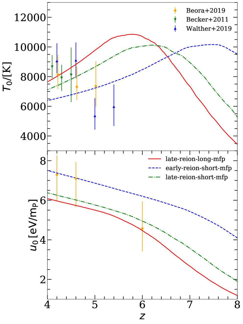
Figure 8: Thermal histories in our three reionization models. Top: Evolution of the gas temperature at mean density of the Universe ($\,T_{\rm 0}\,$). Bottom: Cumulative heating per baryon at the mean density ($\,u_{\rm 0}\,$), which parameterizes the degree of pressure smoothing of the gas. The data points correspond to a selection of recent Ly$\alpha$ forest measurements. Note that our models do not include heating from He$\,\rm\scriptstyle II\$ reionization, which is expected to begin playing a significant role at $z<5$.

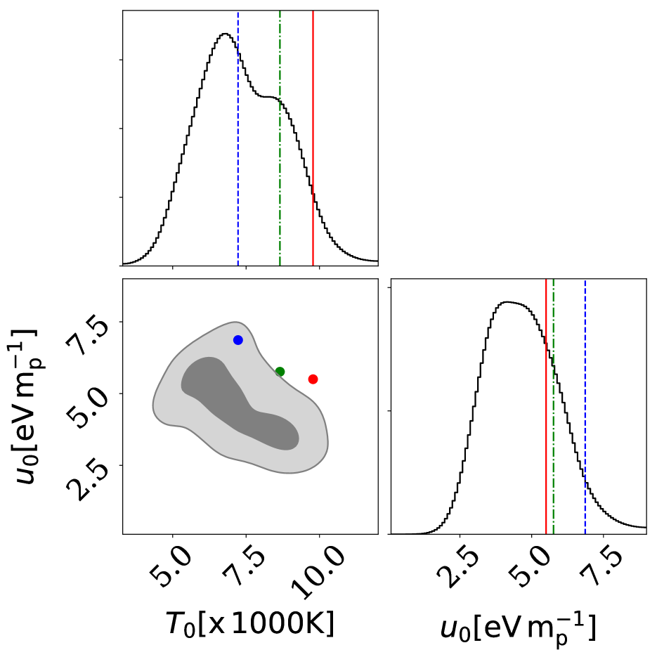
Figure 9: Posterior distributions for the parameters $\,T_{\rm 0}\,$ and $\,u_{\rm 0}\,$ from Boera et al. (2019), obtained from flux power spectrum measurements at $z=5$. The red, blue, and green dots correspond to the late-reion-long-mfp, early-reion-short-mfp, and late-reion-short-mfp models, respectively The grey contours show the 68 and 95 percent credibility regions. The black histograms display the one-dimensional marginalized posterior distributions for the parameters. Note that the evolution of $\,T_{\rm 0}\,$ and $\,u_{\rm 0}\,$ are shown in Fig 8.

As the timing of reionization is different between the “late" and “early" models, a natural starting place is the thermal history of the IGM. Recent studies have pushed Ly$\rm{\alpha}$ forest temperature measurements up to $z\approx 5.4$. These measurements would probe temperatures near overlap in the late reionization scenarios, making them an important consistency check. The top panel of Fig. 8 shows the IGM temperature at the cosmic mean density, $\,T_{\rm 0}\,$, in our three models. For simplicity, we neglect photoheating from He$\,\rm\scriptstyle II\$ionization because (1) our focus is on $z\sim 5$ temperature measurements, and (2) observational constraints suggest that the heating from He$\,\rm\scriptstyle II\$ reionization likely does not pick up until after $z\sim 5$ (see e.g. Schaye et al., 2000; Becker et al., 2011; Walther et al., 2019; Puchwein et al., 2015; Upton Sanderbeck et al., 2016; D’Aloisio et al., 2017; La Plante et al., 2017). We compare our calculations against some of the most recent high-$z$ measurements.

The two late scenarios place the temperature bump, which occurs near the end of reionization, at $z=5.5-6.0$. In these cases we should start to see a rise in temperatures as measurements are pushed towards $z\approx 5.5$. There is, however, no evidence for this rise as of yet. In fact, taken at face value, the measurements disfavor the late reionization models. However, this conclusion comes with two caveats: (1) In formulating our thermal histories, we have adopted the reionization heating calculations of D’Aloisio et al. (2019) based on the I-front speeds in our ESMR reionization models. It is possible that the actual speeds were significantly slower due to the poorly understood role of self-shielded absorbers, which are not captured in our ESMR models (and are likely also not captured in most cosmological radiative transfer simulations). This could have resulted in lower temperatures, particularly near the end of reionization. However, the reduction in I-front speeds would have to be dramatic. To put some numbers to this, lowering I-front speeds by a factor of 20 from $10^{4}$ to $5\times 10^{2}$ proper km/s reduces $T_{\mathrm{reion}}$ from $\approx 27,000K$ to $17,000K$ (D’Aloisio et al., 2019); (2) The state-of-the-art temperature measurements rely on forward-modeling with hydro simulations that do not capture the $\Gamma_{\mathrm{HI}}$ and temperature fluctuations, and inhomogeneous pressure smoothing, from reionization. This could potentially impact the measurements in at least two ways. Firstly, the fluctuations may effectively down-weight the contribution of cold or hot regions to the flux power spectrum, biasing the extracted temperatures. However, previous studies suggest that these effects are likely subtle (Oñorbe et al., 2019; Wu et al., 2019). Secondly, the 1D flux power spectra in early and late reionization models are known to be degenerate; a warm, recently reionized IGM is difficult to distinguish from a cold, pressure-smoothed IGM (see e.g. Wu et al., 2019). The latest measurements account for this degeneracy, but it would be prudent to revisit this topic with more realistic simulations, especially as larger observational data sets are being acquired.

The Ly$\alpha$ forest is sensitive not only to the instantaneous temperature (by Doppler broadening), but also to the reionization thermal history through pressure smoothing of the gas. Recent studies have made progress in disentangling the pressure smoothing effects, which, even at lower redshifts, can be used to constrain reionization in principle. Walther et al. (2019) parameterized the smoothing with a length scale (termed the pressure smoothing scale) that characterizes these effects in the 1D flux power spectrum. Alternatively, Boera et al. (2019) casted these effects into the cumulative heat per proton injected into gas at the mean density, $u_{0}$ (Nasir et al., 2016). Our mock Ly$\alpha$ forest spectra cannot reliably model the small-scale flux power spectrum because our hydro simulation does not have sufficient resolution. Equally important, the pressure smoothing in our models is unrealistic because the inhomogeneous effects of reionization are added in post-processing. We can, however, still get a handle on the pressure smoothing differences between our models by calculating $u_{0}$.

We calculate $u_{0}$ for each mean-density gas parcel in our simulations using that

$$u_{0}=u_{\rm ini,0}+\int_{z_{\rm{o}}}^{z_{\rm{re}}}\frac{\mathscr{H}}{\bar{\rho}}\frac{dz}{H(1+z)},$$ (2)

where $\,u_{\rm ini,0}\,$ corresponds to the impulsive heat injection by an I-front at $z=$$z_{\rm{re}}\,$, and the second term corresponds to the post-reionization photoheating. In the latter, $\bar{\rho}={\rho}_{\rm{crit}}{\Omega}_{\rm{b}}{(1+z)}^{3}$ is the mean baryonic matter density, and $\mathscr{H}$ is the net photoheating rate per unit volume (here for H$\,\rm\scriptstyle I\$ and He$\,\rm\scriptstyle I\$). If the temperature to which the I-front heats the gas is $T_{\rm reion}$, then we take $u_{\rm ini,0}=(3/2)k_{B}T_{\rm reion}/\mu m_{H}$, where we adopt the mean molecular mass of $\mu=0.61$ for ionized hydrogen. Gas parcels are considered to be mean-density if they fall within 2% of $\Delta=1$ and the $\,u_{\rm 0}\,$ that we quote here is averaged over this bin. The bottom panel of Fig. 8 compares our models of $\,u_{\rm 0}\,$ with measurements by Boera et al. (2019). The post-reionization $\,u_{\rm 0}\,$ in early-reion-short-mfp is $\sim 25$ % higher than in the late models owing to the earlier start of reionization. Figure 9 compares our models to the $z=5$ joint posterior distribution of $T_{0}$ and $u_{0}$ from Boera et al. (2019). The contours correspond to 68 and 95 % credibility regions and the red, blue, and green dots correspond to the late-reion-long-mfp, early-reion-short-mfp, and late-reion-short-mfp models, respectively. We note that the models roughly trace the degeneracy direction of the measurements.

In summary, current thermal history measurements do not conclusively favor any our reionization models due to large uncertainties. However, future measurements of the temperature at $z=5.5$ and of the pressure smoothing will likely play an important role in distinguishing between scenarios.

4.2 Ly$\rm{\alpha}$ /Ly$\rm{\beta}$ forest statistics

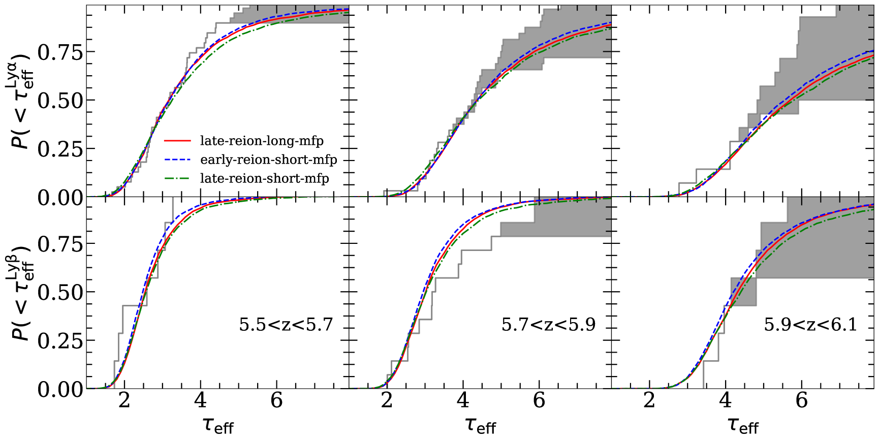
Figure 10: A comparison of Ly$\alpha$ (top) and Ly$\beta$ (bottom) $\tau_{\rm{eff}}\,$ cumulative distributions. The grey histograms show the measurements of Eilers et al. (2019), where the shading spans the “optimistic” and “pessimistic” limits (see text in §3.1 for a description). Following the convention of Eilers et al. (2019), we define $\tau_{\rm{eff}}\,$ by an average over 27 $h^{-1}{\rm Mpc}\,$ segments (as opposed to the $50h^{-1}$ Mpc adopted in the rest of this paper). Our models yield very similar distributions, despite having different global neutral fractions at these redshifts.

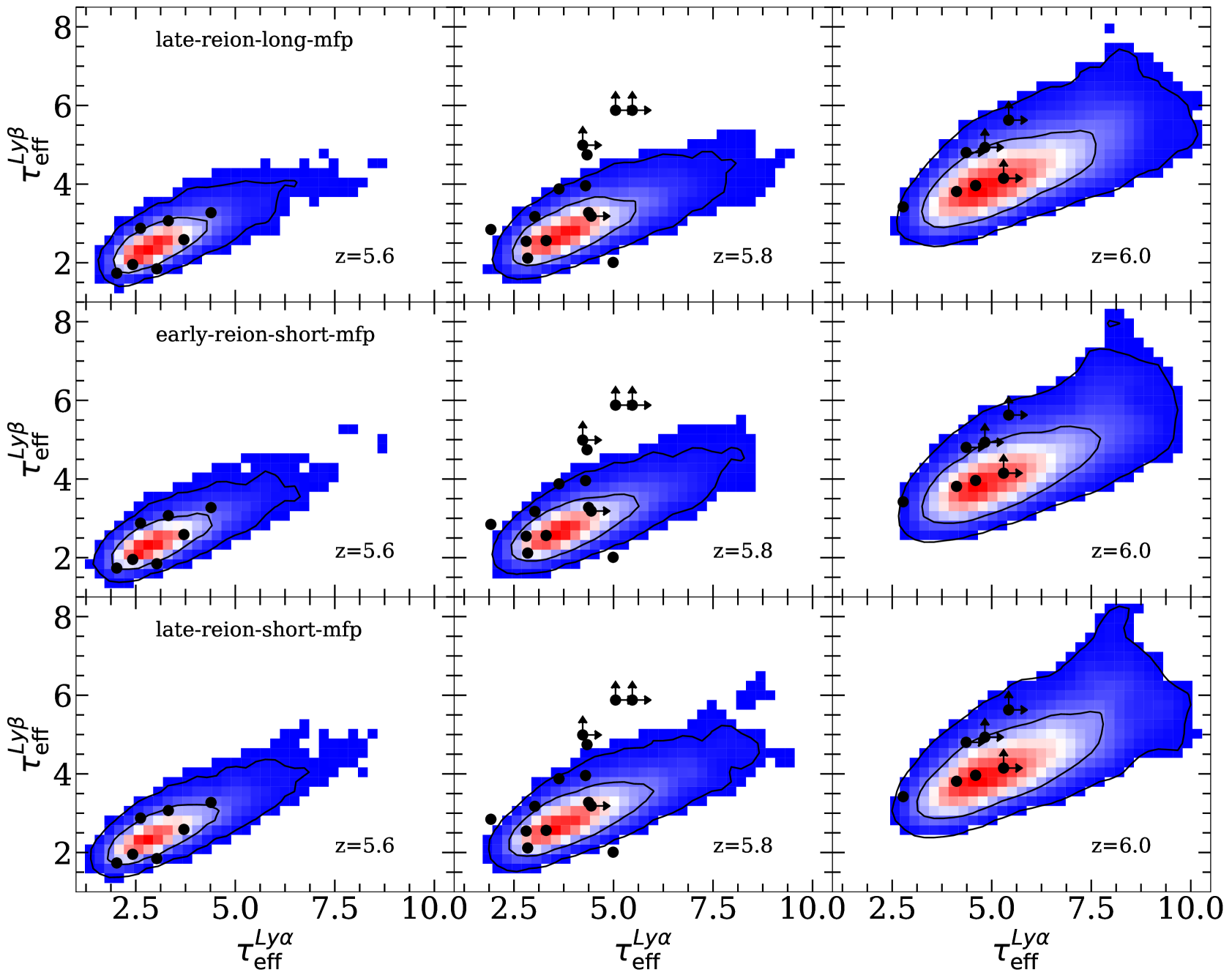
Figure 11: Correlation between Ly$\alpha$ and Ly$\beta$ effective optical depths. Here we define $\tau_{\rm{eff}}\,$ the same way as in Fig. 10. The contours correspond to 68 and 95 percent regions and the data points show the observational measurements of Eilers et al. (2019). The rows show different models while the columns correspond to 3 redshift bins. The models are broadly similar in this correlation.

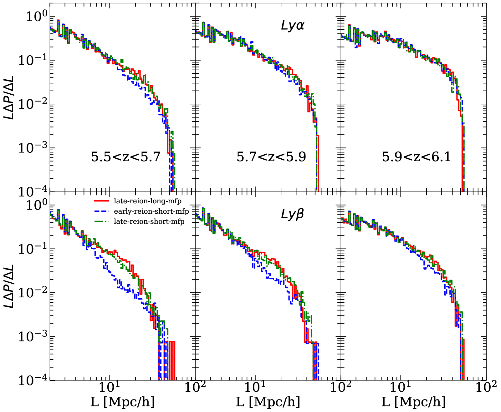
Figure 12: Trough size distributions (or “dark gap distributions") for Ly$\alpha$ (top) and Ly$\beta$ (bottom). In Ly$\alpha$ the distributions are indistinguishable, but in Ly$\beta$ the early-reion-short-mfp model shows fewer troughs of intermediate size ($5\lesssim L\lesssim 20$ $h^{-1}{\rm Mpc}\,$), especially in the $z=5.6$ bin.

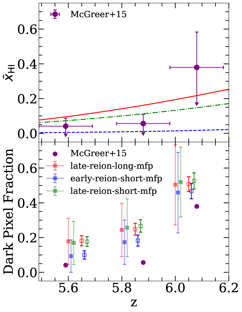
Figure 13: The evolution of the global H$\,\rm\scriptstyle I\$ fraction using the dark pixel fraction. Top panel: The reionization histories of our models compared against 1$\sigma$ upper limits on the neutral fraction measured by McGreer et al. (2015). The upper limits were obtained from dark pixels in the coeval Ly$\alpha$ and Ly$\beta$ forests of their “best sample." Bottom panel: The dark pixel fractions in our mock Ly$\alpha$ and coeval Ly$\beta$ forests. We have matched (approximately) our model spectra to the characteristics of the best sample in McGreer et al. (2015), and we have used their procedure for obtaining H$\,\rm\scriptstyle I\$ fractions. The data points correspond to median values and the error bars display 10th and 90th percentiles, estimated by bootstrap resampling. The closed and open symbols (offset for clear presentation) correspond to using 4 and 100 sight lines per redshift bin, respectively, where the latter corresponds to futuristic measurements. The purple circles show the measurements of McGreer et al. (2015).

4.2.1 Ly$\beta$ opacities

We now turn to Ly$\rm{\alpha}$ and Ly$\rm{\beta}$ forest statistics. We begin with the cumulative distribution of $\tau_{\rm{eff}}\,$ in Ly$\beta$. The Ly$\beta$ opacities are a useful window into the fluctuations because they probe different temperatures and densities. Recently, Eilers et al. (2019) measured this distribution using a sample of 19 quasar sightlines between $5.5\lesssim z\lesssim 6.1$. Particularly at $z\gtrsim 5.8$, they found that fluctuating UVB and temperature models, akin to those of Davies & Furlanetto (2016) and D’Aloisio et al. (2015), under-predict the Ly$\beta$ opacities when they are tuned to match the observed distribution of Ly$\alpha$ opacities. It is interesting to explore this discrepancy further with our models, since they contain neutral islands that can alter the correlation between Ly$\alpha$ and Ly$\beta$ opacities.

In this section we follow the convention of Eilers et al. (2019) in which we measure $\tau_{\rm{eff}}\,$ along segments of length $27h^{-1}$ Mpc, rather than $50h^{-1}$ Mpc. The UVB in our models are iteratively rescaled in the ionized regions to match the Ly$\alpha$ mean fluxes of Eilers et al. (2019), excluding non-detections, and for Ly$\beta$ we include foreground Ly$\alpha$ absorption. To each Ly$\beta$ skewer we add opacities from a randomly chosen skewer from our hydro simulation at $z\approx(1+z_{Ly\alpha})\lambda_{Ly\beta}/\lambda_{Ly\alpha}-1$, where $\lambda_{Ly\beta}$ and $\lambda_{Ly\alpha}$ are the rest-frame Ly$\alpha$ and Ly$\beta$ wavelengths, respectively, and $z_{Ly\alpha}$ is the redshift of interest in the Ly$\alpha$ forest. We rescale the foreground hydro skewers to match the mean fluxes reported by Iršič et al. (2017).

Fig 10 shows a comparison of $\tau_{\rm{eff}}\,$ cumulative distributions for Ly$\alpha$ (top row) and Ly$\beta$ (bottom row) with the measurements of Eilers et al. (2019). All of our models provide reasonable matches to the measurements, with the exception of the $5.7<z<5.9$ bin, where the models do not accommodate the highest Ly$\beta$ opacities observed. Examining the Ly$\beta$ distributions in the 2nd row, the two late reionization models are systematically more opaque than the early model (blue/dashed), but the difference is rather subtle.

We have also examined the correlation between Ly$\alpha$ and Ly$\beta$ $\tau_{\rm{eff}}\,$, as shown in Fig. 11. The contours correspond to 68 and 95 % levels. For this plot, we added noise with $S/N=150$ to roughly match the typical values in Eilers et al. (2019), but we have checked that our conclusion on the similarity of the models is unaffected by the particular choice. Our main conclusions here are: (1) all of the models provide reasonable matches to the data, but they struggle to accommodate the largest Ly$\beta$ opacities in the $z=5.8$ bin; (2) Unfortunately, the models are very similar in these statistics, and we do not find any obvious differences that can help in distinguishing between them.

4.2.2 Trough size distributions

In §3.3 we showed that our models have very similar Ly$\rm{\alpha}$ trough-size distributions. We now examine the trough distributions in Ly$\beta$. It is worth noting that our simulations are likely not converged on the prevalence of transmission peaks, given their sensitivity to fluctuations on extremely small scales. However, we emphasize that our goal here is to search for any obvious qualitative differences between the models. Future models suitable for comparison against data will have to address numerical convergence as well as the in-homogeneity of data sets in spectral resolution and quality.

In Fig. 12, we show the evolution of size distributions in Ly$\alpha$ (top row) and Ly$\beta$ (bottom row). The troughs are extracted using same method as discussed in §3.3, and we also include the effects of evolution in $\Gamma_{\mathrm{HI}}$ over the $\Delta z=0.2$ redshift bins. As in §3.3, the Ly$\alpha$ size distributions are nearly identical. There are some noticeable differences, however, in the Ly$\beta$ distributions. Specifically, the early-reion-short-mfp model (blue/dashed) exhibits a relative deficit of troughs at lengths $5\lesssim L\lesssim 20$ $h^{-1}{\rm Mpc}\,$, particularly in the $5.5<z<5.7$ bin. The deficit of intermediate-size troughs reflects their different physical origin compared to the late models. In the former, the intermediate troughs correspond to highly ionized regions with very low $\Gamma_{\mathrm{HI}}$, whereas in the latter they typically contain extended islands of neutral hydrogen. These differences become more difficult to discern towards higher redshifts as the forest becomes more saturated.

4.2.3 Dark pixel fraction

Lastly, we examine the forest dark pixel fraction, which has been used to place model independent limits on the global neutral fraction at $z\lesssim 6$ (McGreer et al., 2015). Given the difference in neutral fraction at $z\sim 6$ between the late and early scenarios, the dark pixel fraction seems like a natural possibility for distinguishing the models.

The top panel of Fig. 13 compares the 1$\sigma$ upper limits on the neutral fraction of McGreer et al. (2015) against the reionization histories in our models. Another way to compare our models to the measurements is to forward model (to the extent possible) their forest observations and extract an ensemble of mock dark fraction measurements. The distribution of these mock measurements can then be compared against the actual measurements. For this calculation, we rebin to $3.3$ Mpc pixels as in McGreer et al. (2015) and we add a Gaussian noise with ${\rm S/N}=e^{5.5}$ per pixel to mimic the average signal-to-noise of their “best sample." We measure the dark pixel fraction by counting the pixels with negative flux in both Ly$\rm{\alpha}$ and Ly$\rm{\beta}$ simultaneously, and then multiply this number by four. This accounts for the fact that the noise should create upward and downward excursions with equal probability. We use 4 sight lines per redshift bin, roughly similar to the number of sight lines with both Ly$\alpha$ and Ly$\beta$ coverage in the best sample in McGreer et al. (2015). We generate a distribution of mock measurements using $1000$ bootstrap samples. We also explore a “futuristic" scenario assuming 100 sight lines per bin.

In the bottom panel of Fig. 13, we compare the mock dark pixel fraction distributions to the measurements from McGreer et al. (2015) (circles). The squares show median values from our models while the error bars denote 10th and 90th percentiles. The filled and open squares correspond to the current and futuristic scenarios, respectively, where the latter is offset along the x-axis for clarity. The dark pixel fraction is systematically lower in the early-reion-short-mfp model, but only modestly. In fact, the models are again similar in this statistic across all three redshifts, particularly at $z=6$, where one might hope to have the best chance of discerning them. These results suggest that it may be difficult to discern early and late reionization scenarios with dark pixel statistics, even in a futuristic analysis with 100 sight lines per redshift bin, owing to saturation of the forest for ionized regions with low $\Gamma_{\mathrm{HI}}$ in the former. On the other hand, our results suggest that future measurements of the dark pixel fraction could rule out all three models. We note a mild tension between our models and the current measurements, evident in the two lowest redshift bins (compare filled squares with circles).

In summary, we have examined a few Ly$\rm{\alpha}$  and Ly$\rm{\beta}$  forest statistics in search of an easy discriminator for our three distinct reionization scenarios, which have all been tuned to match the mean opacity and scatter in the $z>5.5$ Ly$\alpha$ forest. We found that the models are broadly similar in the statistics that we examined, with the exception of the frequency of intermediate-size ($5\lesssim L\lesssim 20$ $h^{-1}{\rm Mpc}\,$) troughs in the Ly$\beta$ forest.

4.3 Ly$\rm{\alpha}$ emitters

LAEs have emerged as a useful window into the nature of the high-$z$ forest opacity fluctuations (Davies et al., 2018a; Becker et al., 2018). In this section we explore the prospect of distinguishing our models with LAE surveys.

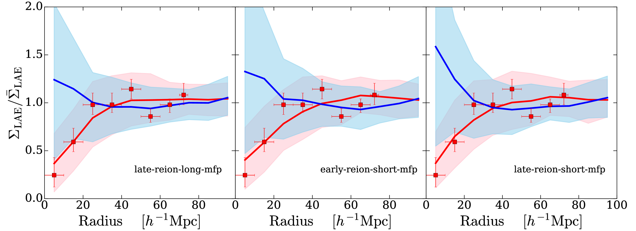
Figure 14: LAE surface densities as a function of radius from transmissive (blue) and opaque (red) sight lines. Surface densities are reported in units of the mean. We select 100 sight lines with the lowest $\tau_{\rm{eff}}\,$ (blue) and 100 with the longest Ly$\alpha$ troughs (red). The curves show the mean surface densities and the shadings show the 10th and 90th percentiles. For reference, the data points show the measurements of Becker et al. (2018) for the extreme Ly$\alpha$ trough in the sightline of J0148.

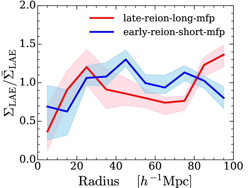
Figure 15: Example sight lines with low $\tau_{\rm{eff}}\,$, but displaying an under-density of LAEs. The shadings span 10 realizations of the LAE population. For both models, we find $\approx 12$ out of 100 sight lines with $\Sigma_{\rm LAE}/\bar{\Sigma}_{\rm LAE}<0.5$ at $R=5$$h^{-1}{\rm Mpc}\,$, indicating that these sight lines are relatively rare. Sight lines of this nature intersect warm voids that were more recently reionized.

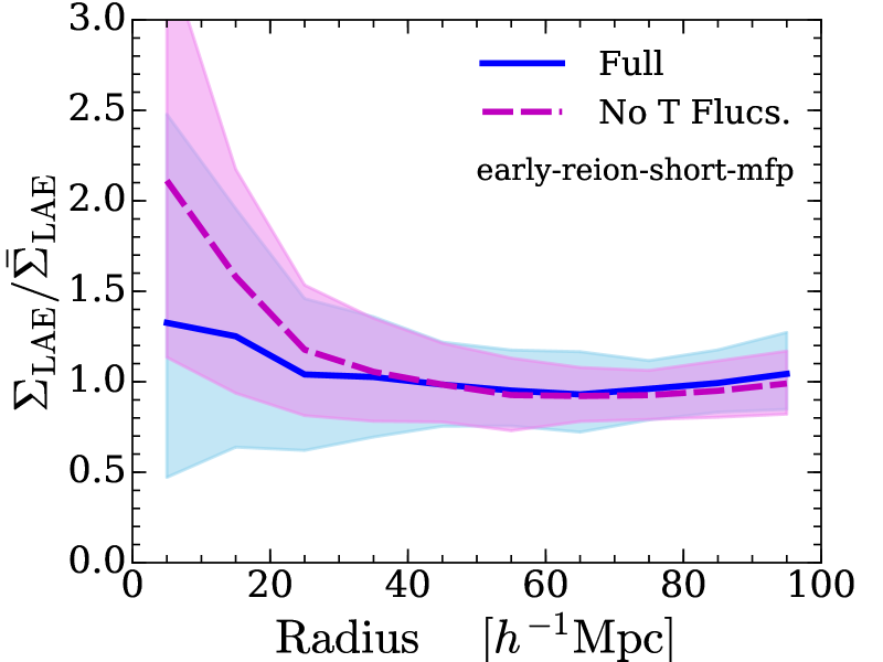
Figure 16: Effect of temperature fluctuations from reionization on the correlation between low-$\tau_{\rm{eff}}\,$and LAE density. For the magenta/dashed curve, we remove the reionization temperature fluctuations and use the original temperatures from our hydro simulation. This effectively assumes that reionization ended early enough for the temperature-density relation to relax to a tight power-law form. Relic temperature fluctuations from reionization create more low-$\tau_{\rm{eff}}\,$ regions out of voids.

Here we mock up LAE surveys along opaque and transmissive forest sight lines in the vein of the recent Hyper Suprime-Cam (HSC) survey towards J0148 by Becker et al. (2018). For each of our three models, we build a sample of the most opaque and transmissive sight lines by identifying the 100 longest Ly$\rm{\alpha}$ troughs, and the 100 most transmissive (lowest $\tau_{\rm{eff}}\,$) segments of length $50$$h^{-1}{\rm Mpc}\,$. For simplicity, in this section we neglect time evolution along the light cone and extract sight lines from our $z=5.8$ snapshot. This simplification is unlikely to alter our statistical conclusions on the correlation with LAE surface density.

We adopt a procedure similar to that in Keating et al. (2019) to generate mock LAE surveys along the extracted sight lines. We abundance match the dark matter halos in our simulation using the UV luminosity function of Bouwens et al. (2015a). We then employ the empirically calibrated model distribution of Dijkstra & Wyithe (2012) to draw rest-frame equivalent widths (REWs) for each halo. The intrinsic spectrum of each galaxy is modeled as a power-law continuum of the form $F_{\lambda}\ \propto\lambda^{-2}$, plus a double-peaked Ly$\rm{\alpha}$ emission line. Following Weinberger et al. (2018), we assume that the component of the emission line blue-ward of systemic is fully attenuated, and we model the red-ward component as a Gaussian with offset of $100~{}\mathrm{km/s}$ and width $\sigma=80~{}\mathrm{km/s}$. We trace skewers of length $150$$h^{-1}{\rm Mpc}\,$from each halo and attenuate the mock spectra according to the opacities along the sight lines. For the late-reionization models, this includes accounting for the damping wing attenuation from neutral hydrogen along the sight line. We then measure the HSC $NB816$ and $i2$ magnitudes using the published transmission curves. We apply two of the three cuts used by Becker et al. (2018), $NB816\leq 26.0$ and $i2-NB816\geq 1.2$, neglecting as in Keating et al. (2019) the $r2$ magnitude cut which extends to redshifts below our modeling. Lastly, as the forest sight lines are drawn at random angles through our box, we rotate the mock LAEs to a head-on view and then bin by transverse radius to measure the surface density profile. This procedure yields a mean LAE surface density of $\approx 0.05~{}(h^{-1}\mathrm{Mpc})^{-2}$, in good agreement with the observed mean surface density in Becker et al. (2018).

In Fig. 14 we show the mean LAE surface density profiles (averaged over 100 sight lines). The red and blue curves correspond to extreme troughs and transmissive segments, respectively. The shading shows the 10th and 90th percentiles in our ensembles. For reference, the red data points show the Becker et al. (2018) measurements for the J0148 trough. For all three models, the surface density profiles towards troughs are consistent with the measurements Becker et al. (2018), reflecting the fact that extreme troughs are generated by voids in these models. In all three models the transmissive regions display a larger scatter in surface densities. More often than not, however, the most transmissive segments of the forest correspond to over-densities in LAEs, even in the late-reion-long-mfp model. One might have guessed that the most transmissive regions in the late-reion-long-mfp model are typically hot, recently reionized voids. Our results suggest that the situation is more complicated when $\Gamma_{\rm HI}$ and temperature fluctuations, and neutral islands, are all at play.

Keating et al. (2019) suggested that the most transmissive sight lines may offer a path to discriminating between models. Whereas the most transmissive (low $\tau_{\rm{eff}}\,$) sight lines typically correspond to over-densities in the model of Davies & Furlanetto (2016), in a late-reionization scenario, at least some of the most transmissive regions should correspond to hot, recently reionized voids. However, Keating et al. (2019) did not quantify how common such transmissive voids are. In our late-reion-long-mfp model we do find transmissive sight lines with a deficit of LAEs, much like the one reported in Keating et al. (2019), but they are relatively rare. For example, 12 out of the 100 transmissive sight lines in our sample have surface densities $\Sigma_{\rm LAE}/\bar{\Sigma}_{\rm LAE}<0.5$ at $R=5$ $h^{-1}{\rm Mpc}\,$. One such sight line is shown as the red curve in Fig. 15, where the shading spans ten realizations of the LAE population (i.e. ten different samples drawn randomly from the REW distribution). However, we also find these under-dense sight lines with similar frequency (13/100) in the early-reion-short-mfp model – one of which is shown as the blue curve in Fig. 15.

At face value, the wide dispersion for transmissive sight lines in our early-reion-short-mfp model appears inconsistent with the tighter correlation between transmission and LAE over-density reported by Davies et al. (2018b). We find that this discrepancy owes to the presence of temperature fluctuations in our early-reion-short-mfp model. To demonstrate this, we remove the reionization temperature fluctuations from the model and use the original temperatures from the hydro simulation. Again, this effectively assumes that reionization was completed early enough for the temperature-density relation to relax to a tight power-law form. The results of this exercise are shown as the magenta/dashed curve in Fig. 16. When we remove the temperature fluctuations we find a tighter correlation between transmission and LAE density, more consistent with the findings of Davies et al. (2018b), who did not include temperature fluctuations from reionization in their model.

Our results suggest that it is difficult to discern our three models by targeting the most transmissive segments of the Ly$\rm{\alpha}$ forest. This difficulty arises from the interplay between $\Gamma_{\rm HI}$ and temperature fluctuations in generating large scatter among the low-$\tau_{\rm{eff}}\,$ sight lines in all three models. On the other hand, if a strong correlation between low-$\tau_{\rm{eff}}\,$ and galaxy/LAE over-densities is measured (ruling out all three of these models), it may be indicative of a relaxed temperature-density relation with minimal scatter, and therefore an earlier end to reionization. Surveys targeting Ly$\rm{\alpha}$ forest sight lines thus remain a potentially insightful window into the physical nature of the fluctuations and ultimately of reionization.

5 Conclusions

Previous studies have noted a marked rise in the scatter of Ly$\alpha$ forest opacities at $z>5.5$. We explored a late-reionization model, in which the neutral fraction is still $\approx 10\%$ at $z=5.5$, and found that it can naturally account for the scatter, including long Ly$\alpha$ troughs with properties similar to the one observed in J0148 by Becker et al. (2015). We attempted to contrast this model with two competing models: (1) An “early" reionization scenario characterized by large fluctuations in the post-reionization UVB. This model is similar to that of Davies & Furlanetto (2016); (2) A separate scenario that blends elements of the Davies & Furlanetto (2016) model with late reionization. The nature of Ly$\alpha$ troughs is different between the models. In our fiducial late-reionization model, every long trough contains neutral islands because they are necessary for generating such large-scale regions with high opacity. However, in the early reionzation scenario, long troughs can occur with or without neutral islands. The opacity fluctuations are instead driven by post-reionization spatial variations in the mean free path and UVB.

We compared Ly$\alpha$ and Ly$\beta$ forest statistics such as the distributions and correlations of $\tau_{\rm{eff}}\,$, trough size distributions, and dark pixel fractions, to look for easy discriminators between the models. We found that the models are broadly similar in these statistics, with the exception of the frequency of intermediate-size ($5\lesssim L\lesssim 20$ $h^{-1}{\rm Mpc}\,$) troughs in the Ly$\beta$ forest. Our early reionization model yields fewer gaps in the Ly$\beta$ forest of these sizes. Motivated by the recent findings of Becker et al. (2018), we also explored LAE surveys centered on the most opaque, and most transmissive, regions of the $z=5.7$ forest. All of our models are consistent with the measured LAE surface densities around the Ly$\alpha$ trough of J0148. The predicted surface densities towards the most transmissive sight lines exhibit a large scatter owing to the interplay between UVB and temperature fluctuations. The amount of scatter is similar between the three models, rendering it difficult to distinguish them with this method. However, if observations instead reveal that transmissive sight lines are overwhelmingly associated with overdensities (ruling out all three of our models), this may indicate a more subdued role for temperature fluctuations, e.g. due to an earlier reionization. The correlation between forest transmission and galaxies/LAEs is an informative window into the nature of IGM fluctuations at these redshifts (Becker et al., 2018; Kakiichi et al., 2018; Kashino et al., 2019).

Among the tests that we considered, perhaps the most promising observational window is the thermal history of the IGM. Models in which reionization ended at $z=5-5.5$ predict significantly hotter temperatures at those redshifts compared with earlier reionization models. On the other hand, the gas density fields exhibit a higher degree of pressure smoothing in the latter. In principle these differences should be detectable in the small-scale structure of the forest if measurements can be extended to $z\approx 5.5$ with high-resolution ($\Delta v\lesssim 30$ km/s), high signal-to-noise ($S/N>15$) quasar spectra. One caveat here is the uncertainty in the contribution of quasars to the UVB at these redshifts, which we have not modeled here. A larger-than-expected quasar contribution can boost temperatures by He$\,\rm\scriptstyle II\$ ionizations, complicating the interpretation for the timing of hydrogren reionization (D’Aloisio et al., 2017).

Another path to probing the nature of the UVB fluctuations is to expand measurements of the mean free path at $z>5$. Reproducing the extreme forest opacities in a model along the lines of Davies & Furlanetto (2016) requires that the global mean free path be at least a factor of 2 lower than current measurements at $z<5.2$ suggest. Such a discrepancy is possible – albeit unlikely – if the existing mean free path measurement at $z\approx 5.2$ is biased significantly by the quasar proximity effect (D’Aloisio et al., 2018). Quasars of lower luminosity would be less impacted by the effect, providing in principle a straightforward way to test for the bias. Because one of the primary differences between our models is the mean free path, we argue that extending direct measurements to include fainter quasars would be another informative step towards diagnosing the origin of the forest opacity fluctuations.

Lastly, our results motivate future improvements to the modeling. The largest differences between earlier and later reionization models probably lie in the small-scale structure of the forest, which we have explored only indirectly here. Future progress requires simulations with larger dynamic range, and that capture the dynamical response of the gas. The current work represents an early step towards exploring the testability of these models.

References

- Bañados et al. (2018) Bañados E., et al., 2018, Nature, 553, 473
- Becker et al. (2011) Becker G. D., Bolton J. S., Haehnelt M. G., Sargent W. L. W., 2011, MNRAS, 410, 1096
- Becker et al. (2015) Becker G. D., Bolton J. S., Madau P., Pettini M., Ryan-Weber E. V., Venemans B. P., 2015, MNRAS, 447, 3402
- Becker et al. (2018) Becker G. D., Davies F. B., Furlanetto S. R., Malkan M. A., Boera E., Douglass C., 2018, ApJ, 863, 92
- Boera et al. (2019) Boera E., Becker G. D., Bolton J. S., Nasir F., 2019, ApJ, 872, 101
- Bond et al. (1991) Bond J. R., Cole S., Efstathiou G., Kaiser N., 1991, ApJ, 379, 440
- Bosman et al. (2018) Bosman S. E. I., Fan X., Jiang L., Reed S., Matsuoka Y., Becker G., Haehnelt M., 2018, MNRAS, 479, 1055
- Bouwens et al. (2015a) Bouwens R. J., et al., 2015a, ApJ, 803, 34
- Bouwens et al. (2015b) Bouwens R. J., Illingworth G. D., Oesch P. A., Caruana J., Holwerda B., Smit R., Wilkins S., 2015b, ApJ, 811, 140
- Chardin et al. (2017) Chardin J., Puchwein E., Haehnelt M. G., 2017, MNRAS, 465, 3429
- D’Aloisio et al. (2015) D’Aloisio A., McQuinn M., Trac H., 2015, ApJ, 813, L38
- D’Aloisio et al. (2017) D’Aloisio A., Upton Sanderbeck P. R., McQuinn M., Trac H., Shapiro P. R., 2017, MNRAS, 468, 4691
- D’Aloisio et al. (2018) D’Aloisio A., McQuinn M., Davies F. B., Furlanetto S. R., 2018, MNRAS, 473, 560
- D’Aloisio et al. (2019) D’Aloisio A., McQuinn M., Maupin O., Davies F. B., Trac H., Fuller S., Upton Sanderbeck P. R., 2019, ApJ, 874, 154
- Davies & Furlanetto (2016) Davies F. B., Furlanetto S. R., 2016, MNRAS, 460, 1328
- Davies et al. (2018a) Davies F. B., Becker G. D., Furlanetto S. R., 2018a, ApJ, 860, 155
- Davies et al. (2018b) Davies F. B., et al., 2018b, ApJ, 864, 142
- Deparis et al. (2019) Deparis N., Aubert D., Ocvirk P., Chardin J., Lewis J., 2019, A&A, 622, A142
- Dijkstra & Wyithe (2012) Dijkstra M., Wyithe J. S. B., 2012, MNRAS, 419, 3181
- Eilers et al. (2018) Eilers A.-C., Davies F. B., Hennawi J. F., 2018, ApJ, 864, 53
- Eilers et al. (2019) Eilers A.-C., Hennawi J. F., Davies F. B., Oñorbe J., 2019, ApJ, 881, 23
- Fan et al. (2006) Fan X., et al., 2006, AJ, 132, 117
- Furlanetto & Oh (2005) Furlanetto S. R., Oh S. P., 2005, MNRAS, 363, 1031
- Furlanetto et al. (2004) Furlanetto S. R., Zaldarriaga M., Hernquist L., 2004, ApJ, 613, 1
- Hui & Gnedin (1997) Hui L., Gnedin N. Y., 1997, MNRAS, 292, 27
- Iršič et al. (2017) Iršič V., et al., 2017, Phys. Rev. D, 96, 023522
- Kakiichi et al. (2018) Kakiichi K., et al., 2018, MNRAS, 479, 43
- Kashino et al. (2019) Kashino D., Lilly S. J., Shibuya T., Ouchi M., Kashikawa N., 2019, arXiv e-prints, p. arXiv:1909.09077
- Keating et al. (2019) Keating L. C., Weinberger L. H., Kulkarni G., Haehnelt M. G., Chardin J., Aubert D., 2019, arXiv e-prints, p. arXiv:1905.12640
- Kulkarni et al. (2019) Kulkarni G., Keating L. C., Haehnelt M. G., Bosman S. E. I., Puchwein E., Chardin J., Aubert D., 2019, MNRAS, 485, L24
- La Plante et al. (2017) La Plante P., Trac H., Croft R., Cen R., 2017, ApJ, 841, 87
- Lacey & Cole (1994) Lacey C., Cole S., 1994, MNRAS, 271, 676
- Lewis et al. (2000) Lewis A., Challinor A., Lasenby A., 2000, ApJ, 538, 473
- Mason et al. (2018) Mason C. A., Treu T., Dijkstra M., Mesinger A., Trenti M., Pentericci L., de Barros S., Vanzella E., 2018, ApJ, 856, 2
- McGreer et al. (2015) McGreer I. D., Mesinger A., D’Odorico V., 2015, MNRAS, 447, 499
- McQuinn & Upton Sanderbeck (2016) McQuinn M., Upton Sanderbeck P. R., 2016, MNRAS, 456, 47
- McQuinn et al. (2011) McQuinn M., Oh S. P., Faucher-Giguère C.-A., 2011, ApJ, 743, 82
- Mesinger et al. (2011) Mesinger A., Furlanetto S., Cen R., 2011, MNRAS, 411, 955
- Miralda-Escudé & Rees (1994) Miralda-Escudé J., Rees M. J., 1994, MNRAS, 266, 343
- Miralda-Escudé et al. (2000) Miralda-Escudé J., Haehnelt M., Rees M. J., 2000, ApJ, 530, 1
- Mortlock et al. (2011) Mortlock D. J., et al., 2011, Nature, 474, 616
- Nasir et al. (2016) Nasir F., Bolton J. S., Becker G. D., 2016, MNRAS, 463, 2335
- Oñorbe et al. (2019) Oñorbe J., Davies F. B., Lukić Z., Hennawi J. F., Sorini D., 2019, MNRAS, 486, 4075
- Planck Collaboration et al. (2018) Planck Collaboration et al., 2018, arXiv e-prints, p. arXiv:1807.06209
- Press & Schechter (1974) Press W. H., Schechter P., 1974, ApJ, 187, 425
- Puchwein et al. (2015) Puchwein E., Bolton J. S., Haehnelt M. G., Madau P., Becker G. D., Haardt F., 2015, MNRAS, 450, 4081
- Schaye et al. (2000) Schaye J., Theuns T., Rauch M., Efstathiou G., Sargent W. L. W., 2000, MNRAS, 318, 817
- Schenker et al. (2012) Schenker M. A., Stark D. P., Ellis R. S., Robertson B. E., Dunlop J. S., McLure R. J., Kneib J.-P., Richard J., 2012, ApJ, 744, 179
- Schmidt et al. (2016) Schmidt K. B., et al., 2016, ApJ, 818, 38
- Songaila (2004) Songaila A., 2004, AJ, 127, 2598
- Tepper-García (2006) Tepper-García T., 2006, MNRAS, 369, 2025
- Trac & Pen (2004) Trac H., Pen U.-L., 2004, New Astronomy, 9, 443
- Trac et al. (2015) Trac H., Cen R., Mansfield P., 2015, ApJ, 813, 54
- Upton Sanderbeck et al. (2016) Upton Sanderbeck P. R., D’Aloisio A., McQuinn M. J., 2016, MNRAS, 460, 1885
- Walther et al. (2019) Walther M., Oñorbe J., Hennawi J. F., Lukić Z., 2019, ApJ, 872, 13
- Weinberger et al. (2018) Weinberger L. H., Kulkarni G., Haehnelt M. G., Choudhury T. R., Puchwein E., 2018, MNRAS, 479, 2564
- Worseck et al. (2014) Worseck G., et al., 2014, MNRAS, 445, 1745
- Wu et al. (2019) Wu X., McQuinn M., Kannan R., D’Aloisio A., Bird S., Marinacci F., Davé R., Hernquist L., 2019, arXiv e-prints, p. arXiv:1907.04860