Accelerating Federated Learning via
Momentum Gradient Descent

Wei Liu, Li Chen, Yunfei Chen, and Wenyi Zhang W. Liu, L. Chen and W. Zhang are with Department of Electronic Engineering and Information Science, University of Science and Technology of China. (e-mail: liuwei93@mail.ustc.edu.cn, {chenli87, wenyizha}@ustc.edu.cn). Y. Chen is with the School of Engineering, University of Warwick, Coventry CV4 7AL, U.K. (e-mail: Yunfei.Chen@warwick.ac.uk).
Abstract

Federated learning (FL) provides a communication-efficient approach to solve machine learning problems concerning distributed data, without sending raw data to a central server. However, existing works on FL only utilize first-order gradient descent (GD) and do not consider the preceding iterations to gradient update which can potentially accelerate convergence. In this paper, we consider momentum term which relates to the last iteration. The proposed momentum federated learning (MFL) uses momentum gradient descent (MGD) in the local update step of FL system. We establish global convergence properties of MFL and derive an upper bound on MFL convergence rate. Comparing the upper bounds on MFL and FL convergence rate, we provide conditions in which MFL accelerates the convergence. For different machine learning models, the convergence performance of MFL is evaluated based on experiments with MNIST dataset. Simulation results comfirm that MFL is globally convergent and further reveal significant convergence improvement over FL.

Index Terms:
accelerated convergence, distributed machine learning, federated learning, momentum gradient descent.

I Introduction

Recently, data-intensive machine learning has been applied in various fields, such as autonomous driving [1], speech recognition [2], image classification [3] and disease detection [4] since this technique provides beneficial solutions to extract the useful information hidden in data. It now becomes a common tendency that machine-learning systems are deploying in architectures that include ten of thousands of processors [5]. Great amount of data is generated by various parallel and distributed physical objects.

Collecting data from edge devices to the central server is necessary for distributed machine learning scenarios. In the process of distributed data collection, there exist significant challenges such as energy efficiency problems and system latency problems. The energy efficiency of distributed data collection was considered in wireless sensor networks (WSNs) due to limited battery capacity of sensors [6]; In fifth-generation (5G) cellular networks, a round-trip delay from terminals through the network back to terminals demands much lower latencies, potentially down to 1 ms, to facilitate human tactile to visual feedback control [7]. Thus, the challenges of data aggregation in distributed system urgently require communication-efficient solutions.

In order to overcome these challenges, cutting down transmission distance and reducing the amount of uploaded data from edge devices to the network center are two effective ways. To reduce transmission distance, mobile edge computing (MEC) in [8] is an emerging technique where the computation and storage resources are pushed to proximity of edge devices where the local task and data offloaded by users can be processed. In this way, the distance of large-scale data transmission is greatly shortened and the latency has a significant reduction [9]. Using machine learning for the prediction of uploaded task execution time achieves a shorter processing delay [10], and dynamic resource scheduling was studied to optimize resources allocation of MEC system in [11]. Moreover, using machine learning to offload computation for MEC can further reduce the computation and communication overhead [12]. To reduce the uploaded data size, model-based compression approaches, where raw data are compressed and represented by well-established model parameters, demonstrate significant compression performance [13]. Lossy compression is also an effective strategy to decrease the uploaded data size [14], [15]. Compressed sensing, where the sparse data of the edge can be efficiently sampled and reconstructed with transmitting a much smaller data size, was applied to data acquisition of Internet of Things (IoT) network [16], [17]. Further, the work in [18] proposed a blockchain-based data sharing to enhance the communication efficiency across resource-limited edges. All the aforementioned works need to collect raw data from individual device.

To avoid collecting raw data for machine learning in distributed scenarios, a novel approach named Federated Learning (FL) has emerged as a promising solution [19]. The work in [20] provided a fundamental architecture design of FL. Considering the growing computation capability of edge nodes (devices), FL decentralizes the centralized machine learning task and assigns the decomposed computing tasks to the edge nodes where the raw data are stored and learned at the edge nodes. After a fixed iteration interval, each edge node transmits its learned model parameter to the central server. This strategy can substantially decrease consumption of communication resources and improve communication-efficiency. To further improve the energy efficiency of FL, the work in [21] proposed an adaptive FL approach, where the aggregation frequency can be adjusted adaptively to minimize the loss function under a fixed resource budget. To reduce the uplink communication costs, the work in [22] proposed structured and sketched updates method, and compression techniques were adopted to reduce parameter dimension in this work. A novel algorithm was proposed to compress edge node updates in [23]. In this algorithm, gradient selection and adaptive adjustment of learning rate were used for efficient compression. For security aggregation of high-dimensional data, the works in [24], [25] provided a communication-efficient approach, where the server can compute the sum of model parameters from edge nodes without knowing the contribution of each individual node. In [26], under unbalanced resource distribution in network edge, FL with client (edge node) selection was proposed for actively managing the clients aggregation according to their resources condition. In [27], non-iid data distribution was studied and a strategy was proposed to improve FL learning performance under this situation.

However, existing FL solutions generally use gradient descent (GD) for loss function minimization. GD is a one-step method where the next iteration depends only on the current gradient. Convergence rate of GD can be improved by accounting for more preceding iterations [28]. Thus, by introducing the last iteration, which is named momentum term, momentum gradient descent (MGD) can accelerate the convergence. The work in [29] gave a theoretical explanation that under the assumption of strong convexity, MGD speeds up the convergence in comparison with GD. Further work in [30] provided conditions in which MGD is globally convergent.

Motivated by the above observation, we propose a new federated learning design of Momentum Federated Learning (MFL) in this paper. In the proposed MFL design, we introduce momentum term in FL local update and leverage MGD to perform local iterations. Further, the global convergence of the proposed MFL is proven. We derive the theoretical convergence bound of MFL. Compared with FL [21], the proposed MFL has an accelerated convergence rate under certain conditions. On the basis of MNIST dataset, we numerically study the proposed MFL and obtain its loss function curve. The experiment results show that MFL converges faster than FL for different machine learning models. The contributions of this paper are summarized as follows:

  • MFL design: According to the characteristic that MGD facilitates machine learning convergence in the centralized situation, we propose MFL design where MGD is adopted to optimize loss function in local update. The proposed MFL can improve the convergence rate of distributed learning problem significantly.

  • Convergence analysis for MFL: We prove that the proposed MFL is globally convergent on convex optimization problems, and derive its theoretical upper bound on convergence rate. We make a comparative analysis of convergence performance between the proposed MFL and FL. It is proven that MFL improves convergence rate of FL under certain conditions.

  • Evaluation based on MNIST dataset: We evaluate the proposed MFL’s convergence performance via simulation based on MNIST dataset with different machine learning models. Then an experimental comparison is made between FL and the proposed MFL. The simulation results show that MFL is globally convergent and confirm that MFL provides a significant improvement of convergence rate.

The remaining part of this paper is organized as follows. We introduce the system model to solve the learning problem in distributed scenarios in Section II and subsequently elaborate the existing solutions in Section III. In Section IV, we describe the design of MFL in detail. Then in Section V and VI, we present the convergence analysis of MFL and the comparison between FL and MFL, respectively. Finally, we show experimentation results in Section VII and draw a conclusion in Section VIII.
Refer to caption
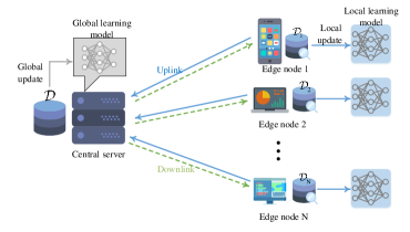
Figure 1: The simplified structure of learning system for distributed user data

II System Model

In this paper, considering a simplified system model, we discuss the distributed network as shown in Fig. 1. This model has N𝑁N edge nodes and a central server. This N𝑁N edge nodes, which have limited communication and computation resources, contain local datasets 𝒟1,𝒟2,,𝒟i,,𝒟Nsubscript𝒟1subscript𝒟2subscript𝒟𝑖subscript𝒟𝑁\mathcal{D}_{1},\mathcal{D}_{2},...,\mathcal{D}_{i},...,\mathcal{D}_{N}, respectively. So the global dataset is 𝒟𝒟1𝒟2𝒟N𝒟subscript𝒟1subscript𝒟2subscript𝒟𝑁\mathcal{D}\triangleq\mathcal{D}_{1}\cup\mathcal{D}_{2}\cup\cdots\cup\mathcal{D}_{N}. Assume that 𝒟i𝒟j=subscript𝒟𝑖subscript𝒟𝑗\mathcal{D}_{i}\cap\mathcal{D}_{j}=\emptyset for ij𝑖𝑗i\neq j. We define the number of samples in node i𝑖i as |𝒟i|subscript𝒟𝑖|\mathcal{D}_{i}| where |||\cdot| denotes the size of the set. The total number of all nodes’ samples is |𝒟|𝒟|\mathcal{D}|, and |𝒟|=i=1N|𝒟i|𝒟superscriptsubscript𝑖1𝑁subscript𝒟𝑖|\mathcal{D}|=\sum_{i=1}^{N}|\mathcal{D}_{i}|. The central server connects all the edge nodes for information transmission.

We define the global loss function at the central server as F(w)𝐹wF(\textbf{w}), where w denotes the model parameter. Different machine learning models correspond to different F()𝐹F(\cdot) and w. We use wsuperscriptw\textbf{w}^{*} to represent the optimal parameter for minimizing the value of F(w)𝐹wF(\textbf{w}). Based on the presented model, the learning problem is to minimize F(w)𝐹wF(\textbf{w}) and it can be formulated as follows:

wargminF(w).superscriptw𝐹w\displaystyle\textbf{w}^{*}\triangleq\mathop{\arg}\mathop{\min}F(\textbf{w}). (1)

Because of the complexity of machine learning model and original dataset, finding a closed-form solution of the above optimization problem is usually impossible. So algorithms based on gradient iterations are used to solve (1). If raw user data are collected and stored in the central server, we can use centralized learning solutions to (1) while if raw user data are distributed over the edge nodes, FL and the proposed MFL can be applied to optimize this learning problem.

Under the situation where FL or MFL solutions are used, the local loss function of node i𝑖i is denoted by Fi(w)subscript𝐹𝑖wF_{i}(\textbf{w}) which is defined merely on 𝒟isubscript𝒟𝑖\mathcal{D}_{i}. Then we define the global loss function F(w)𝐹wF(\textbf{w}) on 𝒟𝒟\mathcal{D} as follows:

Definition 1 (Global loss function).

Given the loss function Fi(w)subscript𝐹𝑖wF_{i}(\textup{{w}}) of edge node i𝑖i, we define the global loss function on all the distributed datasets as

F(w)i=1N|𝒟i|Fi(w)|𝒟|.𝐹wsuperscriptsubscript𝑖1𝑁subscript𝒟𝑖subscript𝐹𝑖w𝒟\displaystyle F(\textup{{w}})\triangleq\frac{\sum_{i=1}^{N}|\mathcal{D}_{i}|F_{i}(\textup{{w}})}{|\mathcal{D}|}. (2)

III Existing Solutions

In this section, we introduce two existing solutions to solve the learning problem expressed by (1). These two solutions are centralized learning solution and FL solution, respectively.

III-A Centralized Learning Solution

Centralized machine learning is for machine learning model embedded in the central server and each edge node needs to send its raw data to the central sever. In this situation, edge nodes will consume communication resources for data transmission, but without incurring computation resources consumption.

After the central server has collected all datasets from the edge nodes, a usual way to solve the learning problem expressed by (1) is GD which globally converges for convex optimization problem. However, due to the one-step nature of GD that each update relates only to the current iteration, the convergence performance of GD still has the potential to be improved by accounting for the history of iterations. There exist multi-step methods where the next update relies not only on the current iteration but also on the preceding ones. MGD is the simplest multi-step method to solve the learning problem of (1) with convergence acceleration. In MGD, each gradient update includes the last iteration which is called the momentum term. It has been proven that MGD improves convergence rate of GD in [29].

III-A1 GD

The update rule for GD is as follows:

w(t)=w(t1)ηF(w(t1)).w𝑡w𝑡1𝜂𝐹w𝑡1\displaystyle\textbf{w}(t)=\textbf{w}(t-1)-\eta\nabla F(\textbf{w}(t-1)). (3)

In (3), t𝑡t denotes the iteration index and η>0𝜂0\eta>0 is the learning step size. The model parameter w is updated along the direction of negative gradient. Using the above update rule, GD can solve the learning problem with continuous iterations.

III-A2 MGD

As an improvement of GD, MGD introduces the momentum term and we present its update rules as follows:

d(t)d𝑡\displaystyle\textbf{d}(t) =γd(t1)+F(w(t1))absent𝛾d𝑡1𝐹w𝑡1\displaystyle=\gamma\textbf{d}(t-1)+\nabla F(\textbf{w}(t-1)) (4)
w(t)w𝑡\displaystyle\textbf{w}(t) =w(t1)ηd(t),absentw𝑡1𝜂d𝑡\displaystyle=\textbf{w}(t-1)-\eta\textbf{d}(t), (5)

where d(t)d𝑡\textbf{d}(t) is the momentum term which has the same dimension as w(t)w𝑡\textbf{w}(t), γ𝛾\gamma is the momentum attenuation factor, η𝜂\eta is the learning step size and t𝑡t is the iteration index. By iterations of (4) and (5) with t𝑡t, F(w)𝐹wF(\textbf{w}) can potentially converge to the minimum faster compared with GD. The convergence range of MGD is 1<γ<11𝛾1-1<\gamma<1 with a bounded η𝜂\eta and if 0<γ<10𝛾10<\gamma<1, MGD has an accelerated convergence rate than GD under a small η𝜂\eta typically used in simulations [31, Result 3].

III-B FL Solution

Collecting and uploading the distributed data are challenging for communication-constrained distributed network. Due to the limited communication resources at edge nodes, the transmission latency of raw user data could be large which deteriorates network feedback performance. Also, the transmission of user data is prone to be at the risk of violating user privacy and security over the entire network. In order to overcome these challenges, FL was proposed as a communication-efficient learning solution without data collection and transmission [19].

In contrast with centralized learning solutions, FL decouples the machine learning task from the central server to each edge node to avoid storing user data in the server and reduce the communication consumption. All of edge nodes make up a federation in coordination with the central server. In FL, each edge node performs local update and transmits its model parameter to the central server after a certain update interval. The central server integrates the received parameters to obtain a globally updated parameter, and sends this parameter back to all the edge nodes for next update interval.

The FL design and convergence analysis are presented in [21] where FL network is studied thoroughly. In an FL system, each edge node uses the same machine learning model. We use τ𝜏\tau to denote the global aggregation frequency, i.e., the update interval. Each node i𝑖i has its local model parameter w~i(t)subscript~w𝑖𝑡\widetilde{\textbf{w}}_{i}(t), where the iteration index is denoted by t=0,1,2,𝑡012t=0,1,2,... (in this paper, an iteration means a local update). We use [k]delimited-[]𝑘[k] to denote the aggregation interval [(k1)τ,kτ]𝑘1𝜏𝑘𝜏[(k-1)\tau,k\tau] for k=1,2,3,𝑘123k=1,2,3,.... At t=0𝑡0t=0, local model parameters of all nodes are initialized to the same value. When t>0𝑡0t>0, w~i(t)subscript~w𝑖𝑡\widetilde{\textbf{w}}_{i}(t) is updated locally based on GD, which is the local update. After τ𝜏\tau local updates, global aggregation is performed and all edge nodes send the updated model parameters to the centralized server synchronously.

The learning process of FL is described as follows.

III-B1 Local Update

When t[k]𝑡delimited-[]𝑘t\in[k], local updates are performed in each edge node by

w~i(t)=w~i(t1)ηFi(w~i(t1)),subscript~w𝑖𝑡subscript~w𝑖𝑡1𝜂subscript𝐹𝑖subscript~w𝑖𝑡1\widetilde{\textbf{w}}_{i}(t)=\widetilde{\textbf{w}}_{i}(t-1)-\eta\nabla F_{i}(\widetilde{\textbf{w}}_{i}(t-1)),

which follows GD exactly.

III-B2 Global Aggregation

When t=kτ𝑡𝑘𝜏t=k\tau, global aggregation is performed. Each node sends w~i(kτ)subscript~w𝑖𝑘𝜏\widetilde{\textbf{w}}_{i}(k\tau) to the central server synchronously. The central server takes a weighted average of the received parameters from N𝑁N nodes to obtain the globally updated parameter w(kτ)w𝑘𝜏\textbf{w}(k\tau) by

w(kτ)=i=1N|𝒟i|w~i(kτ)|𝒟|.w𝑘𝜏superscriptsubscript𝑖1𝑁subscript𝒟𝑖subscript~w𝑖𝑘𝜏𝒟\textbf{w}(k\tau)=\frac{\sum_{i=1}^{N}|\mathcal{D}_{i}|\widetilde{\textbf{w}}_{i}(k\tau)}{|\mathcal{D}|}.

Then w(kτ)w𝑘𝜏\textbf{w}(k\tau) is sent back to all edge nodes as their new parameters and edge nodes perform local update for the next iteration interval.

In [21, Lemma 2], the FL solution has been proven to be globally convergent for convex optimization problems and exhibits good convergence performance. So FL is an effective solution to the distributed learning problem presented in (1).

TABLE I: MFL notation summary
Notation Definition
T𝑇T; K𝐾K; N𝑁N number of total local iterations; number of global aggregations/number of intervals; number of edge nodes
t𝑡t; k𝑘k; τ𝜏\tau; [k]delimited-[]𝑘[k] iteration index; interval index; aggregation frequency with τ=T/K𝜏𝑇𝐾\tau=T/K; the interval [(k1)τ,kτ]𝑘1𝜏𝑘𝜏[(k-1)\tau,k\tau]
wsuperscriptw\textbf{w}^{*}; wfsuperscriptwf\textbf{w}^{\mathrm{f}} global optimal parameter of F()𝐹F(\cdot); the optimal parameter that MFL can obtain in Algorithm 1
η𝜂\eta; β𝛽\beta; ρ𝜌\rho; γ𝛾\gamma the learning step size of MGD or GD; the β𝛽\beta-smooth parameter of Fi()subscript𝐹𝑖F_{i}(\cdot); the ρ𝜌\rho-Lipschitz parameter of Fi()subscript𝐹𝑖F_{i}(\cdot); the momentum attenuation factor which decides the proportion of momentum term in MGD
𝒟isubscript𝒟𝑖\mathcal{D}_{i}; 𝒟𝒟\mathcal{D} the local dataset of node i𝑖i; the global dataset
δisubscript𝛿𝑖\delta_{i}; δ𝛿\delta the upper bound between F(w)𝐹w\nabla F(\textbf{w}) and Fi(w)subscript𝐹𝑖w\nabla F_{i}(\textbf{w}); the average of δisubscript𝛿𝑖\delta_{i} over all nodes
Fi()subscript𝐹𝑖F_{i}(\cdot); F()𝐹F(\cdot) the loss function of node i𝑖i; the global loss function
d(t)d𝑡\textbf{d}(t); w(t)w𝑡\textbf{w}(t) the global momentum parameter at iteration round t𝑡t; the global model parameter at iteration round t𝑡t
d~i(t)subscript~d𝑖𝑡\widetilde{\textbf{d}}_{i}(t); w~i(t)subscript~w𝑖𝑡\widetilde{\textbf{w}}_{i}(t) the local momentum parameter of node i𝑖i at iteration round t𝑡t; the local model parameter at iteration round t𝑡t
d[k](t)subscriptddelimited-[]𝑘𝑡\textbf{d}_{[k]}(t); w[k](t)subscriptwdelimited-[]𝑘𝑡\textbf{w}_{[k]}(t) the momentum parameter of centralized MGD at iteration round t𝑡t in [k]delimited-[]𝑘[k]; the model parameter of centralized MGD at iteration round t𝑡t in [k]delimited-[]𝑘[k]
θ[k](t)subscript𝜃delimited-[]𝑘𝑡\theta_{[k]}(t); θ𝜃\theta; p𝑝p the angle between vector F(w[k](t))𝐹subscriptwdelimited-[]𝑘𝑡\nabla F(\textbf{w}_{[k]}(t)) and d[k](t)subscriptddelimited-[]𝑘𝑡\textbf{d}_{[k]}(t); θ𝜃\theta is the maximum of θ[k](t)subscript𝜃delimited-[]𝑘𝑡\theta_{[k]}(t) for 1kK1𝑘𝐾1\leq k\leq K with t[k]𝑡delimited-[]𝑘t\in[k]; p𝑝p is the maximum ratio of d[k](t)normsubscriptddelimited-[]𝑘𝑡\|\textbf{d}_{[k]}(t)\| and F(w[k](t))norm𝐹subscriptwdelimited-[]𝑘𝑡\|\nabla F(\textbf{w}_{[k]}(t))\| for 1kK1𝑘𝐾1\leq k\leq K with t[k]𝑡delimited-[]𝑘t\in[k]

IV Design of MFL

In this section, we introduce the design of MFL to solve the distributed learning problem shown in (1). We first discuss the motivation of our work. Then we present the design of MFL detailedly and the learning problem based on federated system. The main notations of MFL design and analysis are summarized in Table I.

IV-A Motivation

Since MGD improves the convergence rate of GD [29], we want to apply MGD to local update steps of FL and hope that the proposed MFL will accelerate the convergence rate for federated networks.
Refer to caption
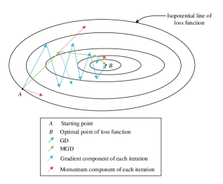
Figure 2: Comparison of MGD and GD

Firstly, we illustrate the intuitive influence on optimization problem after introducing the momentum term into gradient updating methods. Considering GD, the update reduction of the parameter is ηF(w(t1))𝜂𝐹w𝑡1\eta\nabla F(\textbf{w}(t-1)) which is only proportional to the gradient of w(t1)w𝑡1\textbf{w}(t-1). The update direction of GD is always along gradient descent so that an oscillating update path could be caused, as shown by the GD update path in Fig. 2. However, the update reduction of parameter for MGD is a superposition of ηF(w(t1))𝜂𝐹w𝑡1\eta\nabla F(\textbf{w}(t-1)) and γ(w(t2)w(t1))𝛾w𝑡2w𝑡1\gamma(\textbf{w}(t-2)-\textbf{w}(t-1)) which is the momentum term. As shown by the MGD update path in Fig. 2, utilizing the momentum term can deviate the direction of parameter update to the optimal decline significantly and mitigate the oscillation caused by GD. In Fig. 2, GD has an oscillating update path and costs seven iterations to reach the optimal point while MGD only needs three iterations to do that, which demonstrates mitigating the oscillation by MGD leads to a faster convergence rate.

Because edge nodes of distributed networks are usually resource-constrained, solutions to convergence acceleration can attain higher resources utilization efficiency. Thus, motivated by the property that MGD improves convergence rate, we use MGD to perform local update of FL and this approach is named MFL.

In the following subsections, we design the MFL learning paradigm and propose the learning problem based on the MFL design.

IV-B MFL

Refer to caption
Figure 3: Illustration of MFL local update and global aggregation steps from interval [k]delimited-[]𝑘[k] to [k+1]delimited-[]𝑘1[k+1].

In the MFL design, we use d~i(t)subscript~d𝑖𝑡\widetilde{\textbf{d}}_{i}(t) and w~i(t)subscript~w𝑖𝑡\widetilde{\textbf{w}}_{i}(t) to denote momentum parameter and model parameter for node i𝑖i, respectively. All edge nodes are set to embed the same machine learning models. So the local loss functions Fi(w)subscript𝐹𝑖wF_{i}(\textbf{w}) is the same for all nodes, and the dimension of both the model parameters and the momentum parameters are consistent. The parameters setup of MFL is similar to that of FL. We use t𝑡t to denote the local iteration index for t=0,1,𝑡01t=0,1,..., τ𝜏\tau to denote the aggregation frequency and [k]delimited-[]𝑘[k] to denote the interval [(k1)τ,kτ]𝑘1𝜏𝑘𝜏[(k-1)\tau,k\tau] where k𝑘k denotes the interval index for k=1,2,𝑘12k=1,2,.... At t=0𝑡0t=0, the momentum parameters and the model parameters of all nodes are initialized to the same values, respectively. When t[k]𝑡delimited-[]𝑘t\in[k], d~i(t)subscript~d𝑖𝑡\widetilde{\textbf{d}}_{i}(t) and w~i(t)subscript~w𝑖𝑡\widetilde{\textbf{w}}_{i}(t) are updated based on MGD, which is called local update steps. When t=kτ𝑡𝑘𝜏t=k\tau, MFL performs global aggregation steps where d~i(t)subscript~d𝑖𝑡\widetilde{\textbf{d}}_{i}(t) and w~i(t)subscript~w𝑖𝑡\widetilde{\textbf{w}}_{i}(t) are sent to the central server synchronously. Then in the central server, the global momentum parameter d(t)d𝑡\textbf{d}(t) and the global model parameter w(t)w𝑡\textbf{w}(t) are obtained by taking a weighted average of the received parameters, respectively, and are sent back to all edge nodes for the next interval.

The learning rules of MFL include the local update and the global aggregation steps. By continuous alternations of local update and global aggregation, MFL can perform its learning process to minimize the global loss function F(w)𝐹wF(\textbf{w}). We describe the MFL learning process as follows.

First of all, we set initial values for d~i(0)subscript~d𝑖0\widetilde{\textbf{d}}_{i}(0) and w~i(0)subscript~w𝑖0\widetilde{\textbf{w}}_{i}(0). Then

1) Local Update: When t[k]𝑡delimited-[]𝑘t\in[k], local update is performed at each edge node by

d~i(t)subscript~d𝑖𝑡\displaystyle\widetilde{\textbf{d}}_{i}(t) =γd~i(t1)+Fi(w~i(t1))absent𝛾subscript~d𝑖𝑡1subscript𝐹𝑖subscript~w𝑖𝑡1\displaystyle=\gamma\widetilde{\textbf{d}}_{i}(t-1)+\nabla F_{i}(\widetilde{\textbf{w}}_{i}(t-1)) (6)
w~i(t)subscript~w𝑖𝑡\displaystyle\widetilde{\textbf{w}}_{i}(t) =w~i(t1)ηd~i(t).absentsubscript~w𝑖𝑡1𝜂subscript~d𝑖𝑡\displaystyle=\widetilde{\textbf{w}}_{i}(t-1)-\eta\widetilde{\textbf{d}}_{i}(t). (7)

According to (6) and (7), node i𝑖i performs MGD to optimize the loss function Fi()subscript𝐹𝑖F_{i}(\cdot) defined on its own dataset.

2) Global Aggregation: When t=kτ𝑡𝑘𝜏t=k\tau, node i𝑖i transmits w~i(kτ)subscript~w𝑖𝑘𝜏\widetilde{\textbf{w}}_{i}(k\tau) and d~i(kτ)subscript~d𝑖𝑘𝜏\widetilde{\textbf{d}}_{i}(k\tau) to the central server which takes weighted averages of the received parameters from N𝑁N nodes to obtain the global parameters w(kτ)w𝑘𝜏\textbf{w}(k\tau) and d(kτ)d𝑘𝜏\textbf{d}(k\tau), respectively. The aggregation rules are presented as follows:

d(t)d𝑡\displaystyle\textbf{d}(t) =i=1N|𝒟i|d~i(t)|𝒟|absentsuperscriptsubscript𝑖1𝑁subscript𝒟𝑖subscript~d𝑖𝑡𝒟\displaystyle=\frac{\sum_{i=1}^{N}|\mathcal{D}_{i}|\widetilde{\textbf{d}}_{i}(t)}{|\mathcal{D}|} (8)
w(t)w𝑡\displaystyle\textbf{w}(t) =i=1N|𝒟i|w~i(t)|𝒟|.absentsuperscriptsubscript𝑖1𝑁subscript𝒟𝑖subscript~w𝑖𝑡𝒟\displaystyle=\frac{\sum_{i=1}^{N}|\mathcal{D}_{i}|\widetilde{\textbf{w}}_{i}(t)}{|\mathcal{D}|}. (9)

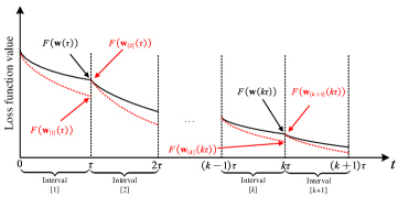
Then the central server sends d(kτ)d𝑘𝜏\textbf{d}(k\tau) and w(kτ)w𝑘𝜏\textbf{w}(k\tau) back to all edge nodes where d~i(kτ)=d(kτ)subscript~d𝑖𝑘𝜏d𝑘𝜏\widetilde{\textbf{d}}_{i}(k\tau)=\textbf{d}(k\tau) and w~i(kτ)=w(kτ)subscript~w𝑖𝑘𝜏w𝑘𝜏\widetilde{\textbf{w}}_{i}(k\tau)=\textbf{w}(k\tau) are set to enable the local update in the next interval [k+1]delimited-[]𝑘1[k+1]. Note that only if t=kτ𝑡𝑘𝜏t=k\tau, the value of the global parameters w(t)w𝑡\textbf{w}(t) and d(t)d𝑡\textbf{d}(t) can be observed. But we define d(t)d𝑡\textbf{d}(t) and w(t)w𝑡\textbf{w}(t) for all t𝑡t to facilitate the following analysis. A typical alternation are shown in Fig. 3 which intuitively illustrates the learning steps of MFL in interval [k]delimited-[]𝑘[k] and [k+1]delimited-[]𝑘1[k+1].

Algorithm 1 MFL The dataset in each node has been set, and the machine learning model embedded in edge nodes has been chosen. We have set appropriate model parameters η𝜂\eta and γ𝛾\gamma.
0:    The limited number of local updates in each node T𝑇TA given aggregation frequency τ𝜏\tau
0:    The final global model weight vector wfsuperscriptwf\textbf{w}^{\mathrm{f}}
1:  Set the initial value of wfsuperscriptwf\textbf{w}^{\mathrm{f}}, w~i(0)subscript~w𝑖0\widetilde{\textbf{w}}_{i}(0) and d~i(0)subscript~d𝑖0\widetilde{\textbf{d}}_{i}(0).
2:  for t=1,2,,T𝑡12𝑇t=1,2,...,T do
3:     Each node i𝑖i performs local update in parallel according to (6) and (7).////Local update
4:     if t==kτt==k\tau where k𝑘k is a positive integer then
5:        Set d~i(t)d(t)subscript~d𝑖𝑡d𝑡\widetilde{\textbf{d}}_{i}(t)\leftarrow\textbf{d}(t) and w~i(t)w(t)subscript~w𝑖𝑡w𝑡\widetilde{\textbf{w}}_{i}(t)\leftarrow\textbf{w}(t) for all nodes where d(t)d𝑡\textbf{d}(t) and w(t)w𝑡\textbf{w}(t) is obtained by (8) and (9) respectively. ////Global aggregationUpdate wfargminw{wf,w(kτ)}F(w)superscriptwfsubscriptwsuperscriptwfw𝑘𝜏𝐹w\textbf{w}^{\mathrm{f}}\leftarrow\mathop{\arg}\mathop{\min}_{\textbf{w}\in\{\textbf{w}^{\mathrm{f}},\textbf{w}(k\tau)\}}F(\textbf{w})
6:     end if
7:  end for

The learning problem of MFL to attain the optimal model parameter is presented as (1). However, the edge nodes have limited computation resources with a finite number of local iterations. We assume that T𝑇T is the number of local iterations and K𝐾K is the corresponding number of global aggregations. Thus, we have tT𝑡𝑇t\leq T and kK𝑘𝐾k\leq K with T=Kτ𝑇𝐾𝜏T=K\tau. Considering that w(t)w𝑡\textbf{w}(t) is unobservable for tkτ𝑡𝑘𝜏t\neq k\tau, we use wfsuperscriptwf\textbf{w}^{\mathrm{f}} to denote the achievable optimal model parameter defined on resource-constrained MFL network. Hence, the learning problem is to obtain wfsuperscriptwf\textbf{w}^{\mathrm{f}} within T𝑇T local iterations particularly, i.e.,

wfargminw{w(kτ):k=1,2,,K}F(w).superscriptwfsubscriptwconditional-setw𝑘𝜏𝑘12𝐾𝐹w\displaystyle\textbf{w}^{\mathrm{f}}\triangleq\mathop{\arg\min}_{\textbf{w}\in\{\textbf{w}(k\tau):k=1,2,...,K\}}F(\textbf{w}). (10)

The optimization algorithm of MFL is explained in Algorithm 1.

V Convergence Analysis

In this section, we firstly make some definitions and assumptions for MFL convergence analysis. Then based on these preliminaries, global convergence properties of MFL following Algorithm 1 are established and an upper bound on MFL convergence rate is derived. Also MFL convergence performance with related parameters is analyzed.

V-A Preliminaries

First of all, to facilitate the analysis, we assume that Fi(w)subscript𝐹𝑖wF_{i}(\textbf{w}) satisfies the following conditions:

Assumption 1.

For Fi(w)subscript𝐹𝑖wF_{i}(\textup{{w}}) in node i𝑖i, we assume the following conditions:
1) Fi(w)subscript𝐹𝑖wF_{i}(\textup{{w}}) is convex
2) Fi(w)subscript𝐹𝑖wF_{i}(\textup{{w}}) is ρ𝜌\rho-Lipschitz, i.e., |Fi(w1)Fi(w2)|ρw1w2subscript𝐹𝑖subscriptw1subscript𝐹𝑖subscriptw2𝜌normsubscriptw1subscriptw2|F_{i}(\textup{{w}}_{1})-F_{i}(\textup{{w}}_{2})|\leq\rho\|\textup{{w}}_{1}-\textup{{w}}_{2}\| for some ρ>0𝜌0\rho>0 and any w1subscriptw1\textup{{w}}_{1}, w2subscriptw2\textup{{w}}_{2}
3) Fi(w)subscript𝐹𝑖wF_{i}(\textup{{w}}) is β𝛽\beta-smooth, i.e., Fi(w1)Fi(w2)βw1w2normsubscript𝐹𝑖subscriptw1subscript𝐹𝑖subscriptw2𝛽normsubscriptw1subscriptw2\|\nabla F_{i}(\textup{{w}}_{1})-\nabla F_{i}(\textup{{w}}_{2})\|\leq\beta\|\textup{{w}}_{1}-\textup{{w}}_{2}\| for some β>0𝛽0\beta>0 and any w1subscriptw1\textup{{w}}_{1}, w2subscriptw2\textup{{w}}_{2}
4) Fi(w)subscript𝐹𝑖wF_{i}(\textup{{w}}) is μ𝜇\mu-strong, i.e., aFi(w1)+(1a)Fi(w2)Fi(aw1+(1a)w2)+a(1a)μ2w1w22𝑎subscript𝐹𝑖subscriptw11𝑎subscript𝐹𝑖subscriptw2subscript𝐹𝑖𝑎subscriptw11𝑎subscriptw2𝑎1𝑎𝜇2superscriptnormsubscriptw1subscriptw22aF_{i}(\textup{{w}}_{1})+(1-a)F_{i}(\textup{{w}}_{2})\geq F_{i}(a\textup{{w}}_{1}+(1-a)\textup{{w}}_{2})+\frac{a(1-a)\mu}{2}\|\textup{{w}}_{1}-\textup{{w}}_{2}\|^{2}, a[0,1]𝑎01a\in[0,1] for some μ>0𝜇0\mu>0 and any w1subscriptw1\textup{{w}}_{1}, w2subscriptw2\textup{{w}}_{2} [32, Theorem 2.1.9]

Because guaranteeing the global convergence of centralized MGD requires that the objective function is strongly convex [29], it is necessary to assume the condition 4. Assumption 1 is satisfied for some learning models such as support vector machine (SVM), linear regression and logistic regression whose loss functions are presented in Table II. From Assumption 1, we can obtain the following lemma:

Lemma 1.

F(w)𝐹wF(\textup{{w}}) is convex, ρ𝜌\rho-Lipschitz, β𝛽\beta-smooth and μ𝜇\mu-strong.

Proof.

According to the definition of F(w)𝐹wF(\textup{{w}}) from (2), triangle inequality and the definition of ρ𝜌\rho-Lipschitz, β𝛽\beta-smooth and μ𝜇\mu-strong, we can derive that F(w)𝐹wF(\textup{{w}}) is convex, ρ𝜌\rho-Lipschitz, β𝛽\beta-smooth and μ𝜇\mu-strong directly. ∎

Then we introduce the gradient divergence between F(w)𝐹w\nabla F(\textbf{w}) and Fi(w)subscript𝐹𝑖w\nabla F_{i}(\textbf{w}) for any node i𝑖i. It comes from the nature of the difference in datasets distribution.

Definition 2 (Gradient divergence).

We define δisubscript𝛿𝑖\delta_{i} as the upper bound between F(w)𝐹w\nabla F(\textup{{w}}) and Fi(w)subscript𝐹𝑖w\nabla F_{i}(\textup{{w}}) for any node i𝑖i, i.e.,

F(w)Fi(w)δi.norm𝐹wsubscript𝐹𝑖wsubscript𝛿𝑖\displaystyle\|\nabla F(\textup{{w}})-\nabla F_{i}(\textup{{w}})\|\leq\delta_{i}. (11)

Also, we define the average gradient divergence

δi|𝒟i|δi|𝒟|.𝛿subscript𝑖subscript𝒟𝑖subscript𝛿𝑖𝒟\displaystyle\delta\triangleq\frac{\sum_{i}|\mathcal{D}_{i}|\delta_{i}}{|\mathcal{D}|}. (12)

Boundedness of δisubscript𝛿𝑖\delta_{i} and δ𝛿\delta: Based on condition 3 of Assumption 1, we let w2=wisubscriptw2superscriptsubscriptw𝑖\textbf{w}_{2}=\textbf{w}_{i}^{*} where wisuperscriptsubscriptw𝑖\textbf{w}_{i}^{*} is the optimal value for minimizing Fi(w)subscript𝐹𝑖wF_{i}(\textbf{w}). Because Fi(w)subscript𝐹𝑖wF_{i}(\textbf{w}) is convex, we have Fi(w1)βw1winormsubscript𝐹𝑖subscriptw1𝛽normsubscriptw1superscriptsubscriptw𝑖\|\nabla F_{i}(\textbf{w}_{1})\|\leq\beta\|\textbf{w}_{1}-\textbf{w}_{i}^{*}\| for any w1subscriptw1\textbf{w}_{1}, which means Fi(w)normsubscript𝐹𝑖w\|\nabla F_{i}(\textbf{w})\| is finite for any w. According to Definition 1 and the linearity of gradient operator, global loss function F(w)𝐹w\nabla F(\textbf{w}) is obtained by taking a weighted average of Fi(w)subscript𝐹𝑖w\nabla F_{i}(\textbf{w}). Therefore, F(w)norm𝐹w\|\nabla F(\textbf{w})\| is finite, and F(w)Fi(w)norm𝐹wsubscript𝐹𝑖w\|\nabla F(\textup{{w}})-\nabla F_{i}(\textup{{w}})\| has an upper bound, i.e., δisubscript𝛿𝑖\delta_{i} is bounded. Further, δ𝛿\delta is still bounded from the linearity in (12).

Since local update steps of MFL perform MGD, the upper bounds of MFL and MGD convergence rate exist certain connections in the same interval. For the convenience of analysis, we use variables d[k](t)subscriptddelimited-[]𝑘𝑡\textbf{d}_{[k]}(t) and w[k](t)subscriptwdelimited-[]𝑘𝑡\textbf{w}_{[k]}(t) to denote the momentum parameter and the model parameter of centralized MGD in each interval [k]delimited-[]𝑘[k], respectively. This centralized MGD is defined on global dataset and updated based on global loss function F(w)𝐹wF(\textbf{w}). In interval [k]delimited-[]𝑘[k], the update rules of centralized MGD follow:

d[k](t)subscriptddelimited-[]𝑘𝑡\displaystyle\textbf{d}_{[k]}(t) =γd[k](t1)+F(w[k](t1))absent𝛾subscriptddelimited-[]𝑘𝑡1𝐹subscriptwdelimited-[]𝑘𝑡1\displaystyle=\gamma\textbf{d}_{[k]}(t-1)+\nabla F(\textbf{w}_{[k]}(t-1)) (13)
w[k](t)subscriptwdelimited-[]𝑘𝑡\displaystyle\textbf{w}_{[k]}(t) =w[k](t1)ηd[k](t).absentsubscriptwdelimited-[]𝑘𝑡1𝜂subscriptddelimited-[]𝑘𝑡\displaystyle=\textbf{w}_{[k]}(t-1)-\eta\textbf{d}_{[k]}(t). (14)

At the beginning of interval [k]delimited-[]𝑘[k], the momentum parameter d[k](t)subscriptddelimited-[]𝑘𝑡\textbf{d}_{[k]}(t) and the model parameter w[k](t)subscriptwdelimited-[]𝑘𝑡\textbf{w}_{[k]}(t) of centralized MGD are synchronized with the corresponding parameters of MFL, i.e.,

d[k]((k1)τ)d((k1)τ)subscriptddelimited-[]𝑘𝑘1𝜏d𝑘1𝜏\displaystyle\textbf{d}_{[k]}((k-1)\tau)\triangleq\textbf{d}((k-1)\tau)
w[k]((k1)τ)w((k1)τ).subscriptwdelimited-[]𝑘𝑘1𝜏w𝑘1𝜏\displaystyle\textbf{w}_{[k]}((k-1)\tau)\triangleq\textbf{w}((k-1)\tau).

For each interval [k]delimited-[]𝑘[k], the centralized MGD is performed by iterations of (13) and (14). In the Fig. 4, we illustrate the distinctions between F(w(t))𝐹w𝑡F(\textbf{w}(t)) and F(w[k](t))𝐹subscriptwdelimited-[]𝑘𝑡F(\textbf{w}_{[k]}(t)) intuitively.

Refer to caption
Figure 4: Illustration of the difference between MGD and MFL in intervals

Comparing with centralized MGD, MFL aggregation interval with τ>1𝜏1\tau>1 brings global update delay because of the fact that centralized MGD performs global update on every iteration while MFL is allowed to spread its global parameter to edge nodes after τ𝜏\tau local updates. Therefore, the convergence performance of MFL is worse than that of MGD, which is essentially from the imbalance between several computation rounds and one communication round in MFL design. The following subsection provides the resulting convergence performance gap between these two approaches.

V-B Gap between MFL and Centralized MGD in Interval [k]delimited-[]𝑘[k]

Firstly, considering a special case, we consider the gap between MFL and centralized MGD for τ=1𝜏1\tau=1. From physical perspective, MFL performs global aggregation after every local update and there does not exist global parameter update delay, i.e, the performance gap is zero. In Appendix A, we prove that MFL is equivalent to MGD for τ=1𝜏1\tau=1 from theoretical perspective.

Now considering general case for any τ1𝜏1\tau\geq 1, the upper bound of gap between w(t)w𝑡\textbf{w}(t) and w[k](t)subscriptwdelimited-[]𝑘𝑡\textbf{w}_{[k]}(t) can be derived as follows.

Proposition 1 (Gap of MFL&\&centralized MGD in intervals).

Given t[k]𝑡delimited-[]𝑘t\in[k], the gap between w(t)w𝑡\textup{{w}}(t) and w[k](t)subscriptwdelimited-[]𝑘𝑡\textup{{w}}_{[k]}(t) can be expressed by

w(t)w[k](t)h(t(k1)τ),normw𝑡subscriptwdelimited-[]𝑘𝑡𝑡𝑘1𝜏\displaystyle\|\textup{{w}}(t)-\textup{{w}}_{[k]}(t)\|\leq h(t-(k-1)\tau), (15)

where we define

A𝐴\displaystyle A (1+γ+ηβ)+(1+γ+ηβ)24γ2γ,absent1𝛾𝜂𝛽superscript1𝛾𝜂𝛽24𝛾2𝛾\displaystyle\triangleq\frac{(1\!+\!\gamma+\!\eta\beta)\!+\!\sqrt{(1\!+\!\gamma\!+\!\eta\beta)^{2}\!-\!4\gamma}}{2\gamma},
B𝐵\displaystyle B (1+γ+ηβ)(1+γ+ηβ)24γ2γ,absent1𝛾𝜂𝛽superscript1𝛾𝜂𝛽24𝛾2𝛾\displaystyle\triangleq\frac{(1\!+\!\gamma+\!\eta\beta)\!-\!\sqrt{(1\!+\!\gamma\!+\!\eta\beta)^{2}\!-\!4\gamma}}{2\gamma},
E𝐸\displaystyle E A(AB)(γA1),absent𝐴𝐴𝐵𝛾𝐴1\displaystyle\triangleq\frac{A}{(A-B)(\gamma A-1)},
F𝐹\displaystyle F B(AB)(1γB)absent𝐵𝐴𝐵1𝛾𝐵\displaystyle\triangleq\frac{B}{(A-B)(1-\gamma B)}

and h(x)𝑥h(x) yields

h(x)𝑥\displaystyle h(x) =ηδ[E(γA)x+F(γB)x1ηβγ(γx1)(γ1)x(γ1)2]absent𝜂𝛿delimited-[]𝐸superscript𝛾𝐴𝑥𝐹superscript𝛾𝐵𝑥1𝜂𝛽𝛾superscript𝛾𝑥1𝛾1𝑥superscript𝛾12\displaystyle\!=\!\eta\delta\left[E(\gamma A)^{x}\!+\!F(\gamma B)^{x}\!-\!\frac{1}{\eta\beta}\!-\!\frac{\gamma(\gamma^{x}-1)-(\gamma-1)x}{(\gamma-1)^{2}}\right] (16)

for 0<γ<10𝛾10<\gamma<1 and any x=0,1,2,𝑥012x=0,1,2,....

Because F(w)𝐹wF(\textup{{w}}) is ρ𝜌\rho-Lipschitz from Lemma 1, it holds that

F(w(t))F(w[k](t))ρh(t(k1)τ).𝐹w𝑡𝐹subscriptwdelimited-[]𝑘𝑡𝜌𝑡𝑘1𝜏\displaystyle F(\textup{{w}}(t))-F(\textup{{w}}_{[k]}(t))\leq\rho h(t-(k-1)\tau). (17)
Proof.

Firstly, we derive an upper bound of w~i(t)w[k](t)normsubscript~w𝑖𝑡subscriptwdelimited-[]𝑘𝑡\|\widetilde{\textbf{w}}_{i}(t)-\textbf{w}_{[k]}(t)\| for node i𝑖i. On the basis of this bound, we extend this result from the local cases to the global one to obtain the final result. The detailed proving process is presented in Appendix B. ∎

Because h(1)=h(0)=0100h(1)=h(0)=0 and h(x)𝑥h(x) increases with x𝑥x for x1𝑥1x\geq 1, which are proven in Appendix C, we always have h(x)0𝑥0h(x)\geq 0 for x=0,1,2,𝑥012x=0,1,2,....

From Proposition 1, in any interval [k]delimited-[]𝑘[k], we have h(0)=000h(0)=0 for t=(k1)τ𝑡𝑘1𝜏t=(k-1)\tau, which fits the definition w[k]((k1)τ)=w((k1)τ)subscriptwdelimited-[]𝑘𝑘1𝜏w𝑘1𝜏\textbf{w}_{[k]}((k-1)\tau)=\textbf{w}((k-1)\tau). We still have h(1)=010h(1)=0 for t=(k1)τ+1𝑡𝑘1𝜏1t=(k-1)\tau+1. This means that there is no gap between MFL and centralized MGD when local update is only performed once after the global aggregation.

It is easy to find that if τ=1𝜏1\tau=1, t(k1)τ𝑡𝑘1𝜏t-(k-1)\tau is either 0 or 1. Because h(1)=h(0)=0100h(1)=h(0)=0, the upper bound in (15) is zero, and there is no gap between F(w(t))𝐹w𝑡F(\textup{{w}}(t)) and F(w[k](t))𝐹subscriptwdelimited-[]𝑘𝑡F(\textup{{w}}_{[k]}(t)) from (17). This is consistent with Appendix A where MFL yields centralized MGD for τ=1𝜏1\tau=1. In any interval [k]delimited-[]𝑘[k], we have t(k1)τ[0,τ]𝑡𝑘1𝜏0𝜏t-(k-1)\tau\in[0,\tau]. If τ>1𝜏1\tau>1, t(k1)τ𝑡𝑘1𝜏t-(k-1)\tau can be larger than 1. When x>1𝑥1x>1, we know that h(x)𝑥h(x) increases with x𝑥x. According to the definition of A𝐴A, B𝐵B, E𝐸E and F𝐹F, we can obtain γA>1𝛾𝐴1\gamma A>1, γB<1𝛾𝐵1\gamma B<1 and E,F>0𝐸𝐹0E,F>0 easily. Because 0<γ<10𝛾10<\gamma<1, the last term will linearly decrease with x𝑥x when x𝑥x is large. Therefore, the first exponential term E(γA)x𝐸superscript𝛾𝐴𝑥E(\gamma A)^{x} in (16) will be dominant when x𝑥x is large and the gap between w(t)w𝑡\textbf{w}(t) and w[k](t)subscriptwdelimited-[]𝑘𝑡\textbf{w}_{[k]}(t) increases exponentially with t𝑡t.

Also we find h(x)𝑥h(x) is proportional to the average gradient gap δ𝛿\delta. It is because the greater the local gradient divergences at different nodes are, the larger the gap will be. So considering the extreme situation where all nodes have the same data samples (δ=0𝛿0\delta=0 because the local loss function are the same), the gap between w(t)w𝑡\textbf{w}(t) and w(t)w𝑡\textbf{w}(t) is zero and MFL is equivalent to centralized MGD.

V-C Global Convergence

We have derived an upper bound between F(w(t))𝐹w𝑡F(\textup{{w}}(t)) and F(w[k](t))𝐹subscriptwdelimited-[]𝑘𝑡F(\textup{{w}}_{[k]}(t)) for t[k]𝑡delimited-[]𝑘t\in[k]. According to the definition of MFL, in the beginning of each interval [k]delimited-[]𝑘[k], we set d[k]((k1)τ)=d((k1)τ)subscriptddelimited-[]𝑘𝑘1𝜏d𝑘1𝜏\textbf{d}_{[k]}((k-1)\tau)=\textbf{d}((k-1)\tau) and w[k]((k1)τ)=w((k1)τ)subscriptwdelimited-[]𝑘𝑘1𝜏w𝑘1𝜏\textbf{w}_{[k]}((k-1)\tau)=\textbf{w}((k-1)\tau). The global upper bound on the convergence rate of MFL can be derived based on Proposition 1.

The following definitions are made to facilitate analysis. Firstly, we use θ[k](t)subscript𝜃delimited-[]𝑘𝑡\theta_{[k]}(t) to denote the angle between vector F(w[k](t)\nabla F(\textbf{w}_{[k]}(t) and d[k](t)subscriptddelimited-[]𝑘𝑡\textbf{d}_{[k]}(t) for t[k]𝑡delimited-[]𝑘t\in[k], i.e.,

cosθ[k](t)F(w[k](t))Td[k](t)F(w[k](t)d[k](t)\cos\theta_{[k]}(t)\triangleq\frac{\nabla F(\textbf{w}_{[k]}(t))^{\mathrm{T}}\textbf{d}_{[k]}(t)}{\|\nabla F(\textbf{w}_{[k]}(t)\|\|\textbf{d}_{[k]}(t)\|}

where θ𝜃\theta is defined as the maximum value of θ[k](t)subscript𝜃delimited-[]𝑘𝑡\theta_{[k]}(t) for 1kK1𝑘𝐾1\leq k\leq K with t[k]𝑡delimited-[]𝑘t\in[k], i.e.,

θmax1kK,t[k]θ[k](t).𝜃subscriptformulae-sequence1𝑘𝐾𝑡delimited-[]𝑘subscript𝜃delimited-[]𝑘𝑡\theta\triangleq\max_{1\leq k\leq K,t\in[k]}\theta_{[k]}(t).

Then we define

pmax1kK,t[k]d[k](t)F(w[k](t))𝑝subscriptformulae-sequence1𝑘𝐾𝑡delimited-[]𝑘normsubscriptddelimited-[]𝑘𝑡norm𝐹subscriptwdelimited-[]𝑘𝑡p\triangleq\max_{1\leq k\leq K,t\in[k]}\frac{\|\textbf{d}_{[k]}(t)\|}{\|\nabla F(\textbf{w}_{[k]}(t))\|}

and

ωmink1w((k1)τ)w2.𝜔subscript𝑘1superscriptnormw𝑘1𝜏superscriptw2\omega\triangleq\min_{k}\frac{1}{\|\textbf{w}((k-1)\tau)-\textbf{w}^{*}\|^{2}}.

Based on Proposition 1 which gives an upper bound of loss function difference between MFL and centralized MGD, global convergence rate of MFL can be derived as follows.

Lemma 2.

If the following conditions are satisfied:
1) cosθ0𝜃0\cos\theta\geq 0, 0<ηβ<10𝜂𝛽10<\eta\beta<1 and 0γ<10𝛾10\leq\gamma<1;
There exists ε>0𝜀0\varepsilon>0 which makes
2) F(w[k](kτ))F(w)ε𝐹subscriptwdelimited-[]𝑘𝑘𝜏𝐹superscriptw𝜀F(\textup{{w}}_{[k]}(k\tau))-F(\textup{{w}}^{*})\geq\varepsilon for all k𝑘k;
3) F(w(T))F(w)ε𝐹w𝑇𝐹superscriptw𝜀F(\textup{{w}}(T))-F(\textup{{w}}^{*})\geq\varepsilon;
4) ωαρh(τ)τε2>0𝜔𝛼𝜌𝜏𝜏superscript𝜀20\omega\alpha-\frac{\rho h(\tau)}{\tau\varepsilon^{2}}>0 hold,
then we have

F(w(T))F(w)1T(ωαρh(τ)τε2)𝐹w𝑇𝐹superscriptw1𝑇𝜔𝛼𝜌𝜏𝜏superscript𝜀2\displaystyle F(\textup{{w}}(T))-F(\textup{{w}}^{*})\leq\frac{1}{T\left(\omega\alpha-\frac{\rho h(\tau)}{\tau\varepsilon^{2}}\right)} (18)

where we defined

αη(1βη2)+ηγ(1βη)cosθβη2γ2p22.𝛼𝜂1𝛽𝜂2𝜂𝛾1𝛽𝜂𝜃𝛽superscript𝜂2superscript𝛾2superscript𝑝22\alpha\triangleq\!\eta(1\!-\!\frac{\beta\eta}{2})\!+\!\eta\gamma(1-\beta\eta)\cos\theta\!-\!\frac{\beta\eta^{2}\gamma^{2}p^{2}}{2}.
Proof.

The proof is presented in Appendix D. ∎

On the basis of Lemma 2, we further derive the following proposition which demonstrates the global convergence of MFL and gives its upper bound on convergence rate.

Proposition 2 (MFL global convergence).

Given cosθ0𝜃0\cos\theta\geq 0, 0<ηβ<10𝜂𝛽10<\eta\beta<1, 0γ<10𝛾10\leq\gamma<1 and α>0𝛼0\alpha>0, we have

F(wf)F(w)12Tωα+14T2ω2α2+ρh(τ)ωατ+ρh(τ).𝐹superscriptwf𝐹superscriptw12𝑇𝜔𝛼14superscript𝑇2superscript𝜔2superscript𝛼2𝜌𝜏𝜔𝛼𝜏𝜌𝜏\displaystyle F(\textup{{w}}^{\mathrm{f}})-F(\textup{{w}}^{*})\leq\frac{1}{2T\omega\alpha}+\sqrt{\frac{1}{4T^{2}\omega^{2}\alpha^{2}}+\frac{\rho h(\tau)}{\omega\alpha\tau}}+\rho h(\tau). (19)
Proof.

The specific proving process is shown in Appendix E. ∎

According to the above Proposition 2, we get an upper bound of F(wf)F(w)𝐹superscriptwf𝐹superscriptwF(\textup{{w}}^{\mathrm{f}})-F(\textup{{w}}^{*}) which is a function of T𝑇T and τ𝜏\tau. From inequality (19), we can find that MFL linearly converges to a lower bound ρh(τ)ωατ+ρh(τ)𝜌𝜏𝜔𝛼𝜏𝜌𝜏\sqrt{\frac{\rho h(\tau)}{\omega\alpha\tau}}+\rho h(\tau). Because h(τ)𝜏h(\tau) is related to τ𝜏\tau and δ𝛿\delta, aggregation intervals (τ>1𝜏1\tau>1) and different data distribution collectively lead to that MFL does not converge to the optimum.

In the following, we discuss the influence of τ𝜏\tau on the convergence bound. If τ=1𝜏1\tau=1, we have ρh(τ)=0𝜌𝜏0\rho h(\tau)=0 so that F(wf)F(w)𝐹superscriptwf𝐹superscriptwF(\textup{{w}}^{\mathrm{f}})-F(\textup{{w}}^{*}) linearly converges to zero as T𝑇T\to\infty, and the convergence rate yields 1Tωα1𝑇𝜔𝛼\frac{1}{T\omega\alpha}. Noting h(τ)>0𝜏0h(\tau)>0 if τ>1𝜏1\tau>1, we can find that in this case, F(wf)F(w)𝐹superscriptwf𝐹superscriptwF(\textup{{w}}^{\mathrm{f}})-F(\textup{{w}}^{*}) converges to a non-zero bound ρh(τ)ωατ+ρh(τ)𝜌𝜏𝜔𝛼𝜏𝜌𝜏\sqrt{\frac{\rho h(\tau)}{\omega\alpha\tau}}+\rho h(\tau) as T𝑇T\to\infty. On the one hand, if there does not exist communication resources limit, setting aggregation frequency τ=1𝜏1\tau=1 and performing global aggregation after each local update can reach the optimal convergence performance of MFL. On the other hand, aggregation interval (τ>1𝜏1\tau>1) can let MFL effectively utilize the communication resources of each node, but bring about a decline of convergence performance.

VI Comparison Between FL and MFL

In this section, we make a comparison of convergence performance between MFL and FL.

The closed-form solution of the upper bound on FL convergence rate has been derived in [21, Theorem 2]. It is presented as follows.

F(wFLf)F(w)12ηφT+14η2φ2T2+ρhFL(τ)ηφτ+ρhFL(τ).𝐹superscriptsubscriptw𝐹𝐿f𝐹superscriptw12𝜂𝜑𝑇14superscript𝜂2superscript𝜑2superscript𝑇2𝜌subscript𝐹𝐿𝜏𝜂𝜑𝜏𝜌subscript𝐹𝐿𝜏\displaystyle F(\textbf{w}_{F\!L}^{\mathrm{f}})\!-\!F(\textup{{w}}^{*})\!\leq\!\frac{1}{2\eta\varphi T}\!+\!\sqrt{\frac{1}{4\eta^{2}\varphi^{2}T^{2}}\!+\!\frac{\rho h_{F\!L}(\tau)}{\eta\varphi\tau}}\!+\!\rho h_{F\!L}(\tau). (20)

According to [21],

hFL(τ)=δβ((ηβ+1)τ1)ηδτsubscript𝐹𝐿𝜏𝛿𝛽superscript𝜂𝛽1𝜏1𝜂𝛿𝜏h_{F\!L}(\tau)=\frac{\delta}{\beta}((\eta\beta+1)^{\tau}-1)-\eta\delta\tau

and φ=ωFL(1ηβ2)𝜑subscript𝜔𝐹𝐿1𝜂𝛽2\varphi=\omega_{F\!L}(1-\frac{\eta\beta}{2}) where the expression of ωFLsubscript𝜔𝐹𝐿\omega_{FL} is consistent with ω𝜔\omega. Differing from that of ω𝜔\omega, w((k1)τ)w𝑘1𝜏\textbf{w}((k-1)\tau) in the definition of ωFLsubscript𝜔𝐹𝐿\omega_{FL} is the global model parameter of FL.

We assume that both MFL and FL solutions are applied in the system model proposed in Fig. 1. They are trained based on the same training dataset with the same machine learning model. The loss function Fi()subscript𝐹𝑖F_{i}(\cdot) and global loss function F()𝐹F(\cdot) of MFL and FL are the same, respective. The corresponding parameters of MFL and FL are equivalent including τ𝜏\tau, η𝜂\eta, ρ𝜌\rho, δ𝛿\delta and β𝛽\beta. We set the same initial value w(0)w0\textbf{w}(0) of MFL and FL. Because both MFL and FL are convergent, we have ω=1w(0)w2𝜔1superscriptnormw0superscriptw2\omega=\frac{1}{\|\textbf{w}(0)-\textbf{w}^{*}\|^{2}}. Then according to the definitions of ω𝜔\omega and ωFLsubscript𝜔𝐹𝐿\omega_{F\!L}, we have w=wFL𝑤subscript𝑤𝐹𝐿w=w_{F\!L}. Therefore, the corresponding parameters of MFL and FL are the same and we can compare the convergences between FL and MFL conveniently.

For convenience, we use f1(T)subscript𝑓1𝑇f_{1}(T) and f2(T)subscript𝑓2𝑇f_{2}(T) to denote the upper bound on convergence rate of MFL and FL, respectively. Then we have

f1(T)12Tωα+14T2ω2α2+ρh(τ)ωατ+ρh(τ)subscript𝑓1𝑇12𝑇𝜔𝛼14superscript𝑇2superscript𝜔2superscript𝛼2𝜌𝜏𝜔𝛼𝜏𝜌𝜏\displaystyle f_{1}(T)\triangleq\frac{1}{2T\omega\alpha}+\sqrt{\frac{1}{4T^{2}\omega^{2}\alpha^{2}}+\frac{\rho h(\tau)}{\omega\alpha\tau}}+\rho h(\tau) (21)

and

f2(T)12ηφT+14η2φ2T2+ρhFL(τ)ηφτ+ρhFL(τ).subscript𝑓2𝑇12𝜂𝜑𝑇14superscript𝜂2superscript𝜑2superscript𝑇2𝜌subscript𝐹𝐿𝜏𝜂𝜑𝜏𝜌subscript𝐹𝐿𝜏\displaystyle f_{2}(T)\triangleq\frac{1}{2\eta\varphi T}\!+\!\sqrt{\frac{1}{4\eta^{2}\varphi^{2}T^{2}}\!+\!\frac{\rho h_{F\!L}(\tau)}{\eta\varphi\tau}}\!+\!\rho h_{F\!L}(\tau). (22)

We consider the special case of γ0𝛾0\gamma\to 0. For ωα𝜔𝛼\omega\alpha and ηφ𝜂𝜑\eta\varphi, we can obtain ωαωη(1βη2)=ηφ𝜔𝛼𝜔𝜂1𝛽𝜂2𝜂𝜑\omega\alpha\to\omega\eta(1-\frac{\beta\eta}{2})=\eta\varphi from the definition of α𝛼\alpha. Then for h(τ)𝜏h(\tau) and hFL(τ)subscript𝐹𝐿𝜏h_{FL}(\tau), we have γAηβ+1𝛾𝐴𝜂𝛽1\gamma A\to\eta\beta+1 and γB0𝛾𝐵0\gamma B\to 0. Because AAB1𝐴𝐴𝐵1\frac{A}{A-B}\to 1 and BAB0𝐵𝐴𝐵0\frac{B}{A-B}\to 0, we can further get E1ηβ𝐸1𝜂𝛽E\to\frac{1}{\eta\beta} and F0𝐹0F\to 0 from the definitions of E𝐸E and F𝐹F. So, according to (16), we have

limγ0h(τ)subscript𝛾0𝜏\displaystyle\lim_{\gamma\to 0}h(\tau) =ηδ[1ηβ(ηβ+1)τ1ηβτ]absent𝜂𝛿delimited-[]1𝜂𝛽superscript𝜂𝛽1𝜏1𝜂𝛽𝜏\displaystyle=\eta\delta\left[\frac{1}{\eta\beta}(\eta\beta+1)^{\tau}\!-\!\frac{1}{\eta\beta}\!-\tau\right]
=δβ((1+ηβ)τ1)ηδτ=hFL(τ).absent𝛿𝛽superscript1𝜂𝛽𝜏1𝜂𝛿𝜏subscript𝐹𝐿𝜏\displaystyle=\frac{\delta}{\beta}((1+\eta\beta)^{\tau}-1)-\eta\delta\tau=h_{FL}(\tau).

Hence, by the above analysis under γ0𝛾0\gamma\to 0, we can find MFL and FL have the same upper bound on convergence rate. This fact is consistent with the property that if γ=0𝛾0\gamma=0, MFL degenerates into FL and has the same convergence rate with FL.

To avoid complicated calculations over the expressions of f1(T)subscript𝑓1𝑇f_{1}(T) and f2(T)subscript𝑓2𝑇f_{2}(T), we consider the special case of small η𝜂\eta (η0𝜂0\eta\to 0) which is typically used in simulations.

Lemma 3.

If η0𝜂0\eta\to 0, existing T11subscript𝑇11T_{1}\geq 1, we have 12Tωα12𝑇𝜔𝛼\frac{1}{2T\omega\alpha} dominates in f1(T)subscript𝑓1𝑇f_{1}(T) and 12ηφT12𝜂𝜑𝑇\frac{1}{2\eta\varphi T} dominates in f2(T)subscript𝑓2𝑇f_{2}(T) for T<T1𝑇subscript𝑇1T<T_{1}, i.e.,

12Tωαmax{ρh(τ),ρh(τ)ωατ}much-greater-than12𝑇𝜔𝛼𝜌𝜏𝜌𝜏𝜔𝛼𝜏\frac{1}{2T\omega\alpha}\gg\max\left\{\rho h(\tau),\sqrt{\frac{\rho h(\tau)}{\omega\alpha\tau}}\right\}

and

12ηφTmax{ρhFL(τ),ρhFL(τ)ηφτ}.much-greater-than12𝜂𝜑𝑇𝜌subscript𝐹𝐿𝜏𝜌subscript𝐹𝐿𝜏𝜂𝜑𝜏\frac{1}{2\eta\varphi T}\gg\max\left\{\rho h_{FL}(\tau),\sqrt{\frac{\rho h_{FL}(\tau)}{\eta\varphi\tau}}\right\}.

Then we have

f1(T)1Tωαsubscript𝑓1𝑇1𝑇𝜔𝛼f_{1}(T)\approx\frac{1}{T\omega\alpha}

and

f2(T)1Tηφsubscript𝑓2𝑇1𝑇𝜂𝜑f_{2}(T)\approx\frac{1}{T\eta\varphi}

for T<T1𝑇subscript𝑇1T<T_{1}.

Proof.

Considering (21), if η0𝜂0\eta\to 0, we have α0𝛼0\alpha\to 0 from the definition of α𝛼\alpha and h(τ)0𝜏0h(\tau)\to 0 from Appendix F. So we can easily derive ωαρh(τ)0𝜔𝛼𝜌𝜏0\omega\alpha\rho h(\tau)\to 0 and ωαρh(τ)τ0𝜔𝛼𝜌𝜏𝜏0\sqrt{\frac{\omega\alpha\rho h(\tau)}{\tau}}\to 0. Then we can find T11subscript𝑇11T_{1}\geq 1 which satisfies 12Tωαρh(τ)much-greater-than12𝑇𝜔𝛼𝜌𝜏\frac{1}{2T}\gg\omega\alpha\rho h(\tau) and 12Tωαρh(τ)τmuch-greater-than12𝑇𝜔𝛼𝜌𝜏𝜏\frac{1}{2T}\gg\sqrt{\frac{\omega\alpha\rho h(\tau)}{\tau}} for T<T1𝑇subscript𝑇1T<T_{1}. Hence, we have 12Tωα12𝑇𝜔𝛼\frac{1}{2T\omega\alpha} dominates in f1(T)subscript𝑓1𝑇f_{1}(T) and f1(T)1Tωαsubscript𝑓1𝑇1𝑇𝜔𝛼f_{1}(T)\approx\frac{1}{T\omega\alpha}.

For the same reason, considering (22), if η0𝜂0\eta\to 0, we have ηφ0𝜂𝜑0\eta\varphi\to 0 from the definition of φ𝜑\varphi and hFL(τ)0subscript𝐹𝐿𝜏0h_{FL}(\tau)\to 0 from its definition. So we can easily derive ηφρhFL(τ)0𝜂𝜑𝜌subscript𝐹𝐿𝜏0\eta\varphi\rho h_{FL}(\tau)\to 0 and ηφρhFL(τ)τ0𝜂𝜑𝜌subscript𝐹𝐿𝜏𝜏0\sqrt{\frac{\eta\varphi\rho h_{FL}(\tau)}{\tau}}\to 0. Then for T<T1𝑇subscript𝑇1T<T_{1}, 12TηφρhFL(τ)much-greater-than12𝑇𝜂𝜑𝜌subscript𝐹𝐿𝜏\frac{1}{2T}\gg\eta\varphi\rho h_{FL}(\tau) and 12TηφρhFL(τ)τmuch-greater-than12𝑇𝜂𝜑𝜌subscript𝐹𝐿𝜏𝜏\frac{1}{2T}\gg\sqrt{\frac{\eta\varphi\rho h_{FL}(\tau)}{\tau}}. Hence, we have 12ηφT12𝜂𝜑𝑇\frac{1}{2\eta\varphi T} dominates in f2(T)subscript𝑓2𝑇f_{2}(T) and f2(T)1Tηφsubscript𝑓2𝑇1𝑇𝜂𝜑f_{2}(T)\approx\frac{1}{T\eta\varphi}. ∎

From Lemma 3, we can find that if the learning step size is small and the local update index is not too large, the influence of the update intervals on convergence rate can be ignored. So taking this property into account, we can set a small learning step size to cut down communication resources consumption by increasing computation resources cost.

Proposition 3 (Accelerated convergence of MFL).

If the following conditions are satisfied:
1) η0𝜂0\eta\to 0;
2) T<T1𝑇subscript𝑇1T<T_{1};
3) 0<γ<10𝛾10<\gamma<1,
MFL converges faster than FL, i.e.,

f1(T)<f2(T).subscript𝑓1𝑇subscript𝑓2𝑇f_{1}(T)<f_{2}(T).
Proof.

From condition 1 and condition 2, we have f1(T)1Tωαsubscript𝑓1𝑇1𝑇𝜔𝛼f_{1}(T)\approx\frac{1}{T\omega\alpha} and f2(T)1Tηφsubscript𝑓2𝑇1𝑇𝜂𝜑f_{2}(T)\approx\frac{1}{T\eta\varphi}. Due to the definition of α𝛼\alpha and φ𝜑\varphi, inequality 0<γ<2(1βη)cosθβηp20𝛾21𝛽𝜂𝜃𝛽𝜂superscript𝑝20<\gamma<\frac{2(1-\beta\eta)\cos\theta}{\beta\eta p^{2}} is equivalent to ωα>ηφ𝜔𝛼𝜂𝜑\omega\alpha>\eta\varphi. So if ωα>ηφ𝜔𝛼𝜂𝜑\omega\alpha>\eta\varphi, it is obvious that 1Tωα<1Tηφ1𝑇𝜔𝛼1𝑇𝜂𝜑\frac{1}{T\omega\alpha}<\frac{1}{T\eta\varphi}, i.e., f1(T)<f2(T)subscript𝑓1𝑇subscript𝑓2𝑇f_{1}(T)<f_{2}(T). From condition 1, 2(1βη)cosθβηp221𝛽𝜂𝜃𝛽𝜂superscript𝑝2\frac{2(1-\beta\eta)\cos\theta}{\beta\eta p^{2}} is larger than 1 definitely. So condition 3 is the range of MFL convergence acceleration after combining with MGD convergence guarantee 0<γ<10𝛾10<\gamma<1.

Refer to caption
(a) SVM
Refer to caption
(b) SVM
Refer to caption
(c) Linear regression
Refer to caption
(d) Logistic regression
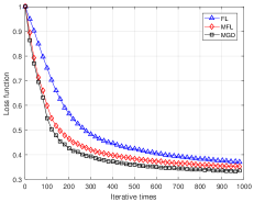
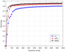
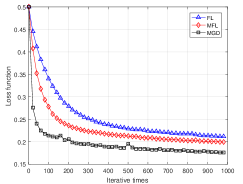
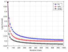
Figure 5: Loss function values and testing accuracy under FL, MFL and MGD. (a) and (b) are the loss function and test accuracy curve of SVM, respectively; (c) and (d) are the loss function curves of linear regression and logistic regression, respectively.

VII Simulation and discussion

In this section, we build and evaluate MFL system based on MNIST dataset. We first describe the simulation environment and the relevant sets of parameters. Then, we present and evaluate the comparative simulation results of MFL, FL and MGD under different machine learning models. Finally, the extensive experiments are implemented to explore the impact of γ𝛾\gamma and τ𝜏\tau on MFL convergence performance.

VII-A Simulation Setup

Using the Python, we build a federated network framework where distributed edge nodes coordinate with the central server. In our network, the number of edge nodes can be chosen arbitrarily. SVM, linear regression and logistic regression can be chosen for model training. Their loss functions at node i𝑖i are presented as in Table II [33]. Note that |𝒟i|subscript𝒟𝑖|\mathcal{D}_{i}| is the number of training samples in node i𝑖i and the loss function of logistic regression is cross-entropy. For logistic regression, model output σ(w,xj)𝜎wsubscriptx𝑗\sigma(\textbf{w},\textbf{x}_{j}) is sigmoid function for non-linear transform. It is defined by

σ(w,xj)11+ewTxj.𝜎wsubscriptx𝑗11superscript𝑒superscriptwTsubscriptx𝑗\displaystyle\sigma(\textbf{w},\textbf{x}_{j})\triangleq\frac{1}{1+e^{-\textbf{w}^{\mathrm{T}}\textbf{x}_{j}}}. (23)
TABLE II: Loss function of three machine learning models
Model Loss function
SVM λ2w2+12|𝒟i|jmax{0;1yjwTxj}𝜆2superscriptnormw212subscript𝒟𝑖subscript𝑗01subscript𝑦𝑗superscriptwTsubscriptx𝑗\frac{\lambda}{2}\|\textbf{w}\|^{2}+\frac{1}{2|\mathcal{D}_{i}|}\sum_{j}\max\{0;1-y_{j}\textbf{w}^{\mathrm{T}}\textbf{x}_{j}\}
Linear regression 12|𝒟i|jyjwTxj212subscript𝒟𝑖subscript𝑗superscriptnormsubscript𝑦𝑗superscriptwTsubscriptx𝑗2\frac{1}{2|\mathcal{D}_{i}|}\sum_{j}\|y_{j}-\textbf{w}^{\mathrm{T}}\textbf{x}_{j}\|^{2}
Logistic regression 1|𝒟i|jyjlogσ(w,xj)+(1yj)log(1σ(w,xj))1subscript𝒟𝑖subscript𝑗normsubscript𝑦𝑗𝜎wsubscriptx𝑗1subscript𝑦𝑗1𝜎wsubscriptx𝑗-\!\frac{1}{|\mathcal{D}_{i}|}\!\sum_{j}\!\|\!y_{j}\!\log\sigma(\textbf{w},\textbf{x}_{j})\!+\!(1\!-\!y_{j})\log(1\!-\!\sigma(\textbf{w},\textbf{x}_{j}))\| where σ(w,xj)𝜎wsubscriptx𝑗\sigma(\textbf{w},\textbf{x}_{j}) is given as (23)
Refer to caption
Refer to caption
Refer to caption
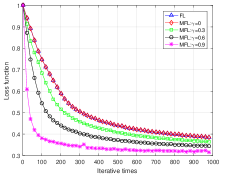
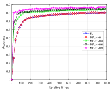
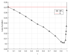
Figure 6: The influence of γ𝛾\gamma on MFL convergence. (a)Loss function values with iterative times under different γ𝛾\gamma; (b)Testing accuracy with iterative times under different γ𝛾\gamma; (c)Loss function values with γ𝛾\gamma when T=1000𝑇1000T=1000.

These three models are trained and tested on MNIST dataset which contains 50,000 training handwritten digits and 10,000 testing handwritten digits. In our experiments, we only utilize 5,000 training samples and 5,000 testing samples because of the limited processing capacities of GD and MGD. In this dataset, the j𝑗j-th sample xjsubscriptx𝑗\textbf{x}_{j} is a 784-dimensional input vector which is vectorized from 28×28282828\times 28 pixel matrix and yjsubscript𝑦𝑗y_{j} is the scalar label corresponding to xjsubscriptx𝑗\textbf{x}_{j}. SVM, linear and logistic regression are used to classify whether the digit is even or odd.

In our experimentation, training and testing samples are randomly allocated to each node, which means the information of each node is uniform. We also simulate FL and centralized MGD as benchmarks. For experimental sets, the system model is set to 4 edge nodes. If the image of xjsubscriptx𝑗\textbf{x}_{j} represents an even number, then we set yj=1subscript𝑦𝑗1y_{j}=1. Otherwise, yj=1subscript𝑦𝑗1y_{j}=-1. But for logistic regression, we set yj=1subscript𝑦𝑗1y_{j}=1 for the even number and yj=0subscript𝑦𝑗0y_{j}=0 for the odd. The same initializations of model parameters are performed and the same data distributions are set for MFL and FL. Also di(0)=0subscriptd𝑖00\textbf{d}_{i}(0)=\textbf{0} is set for node i𝑖i. We set the learning step size η=0.002𝜂0.002\eta=0.002 which is sufficiently small, SVM parameter λ=0.3𝜆0.3\lambda=0.3 and the total number of local iterations T=1,000𝑇1000T=1,000 for the following simulations.

Refer to caption
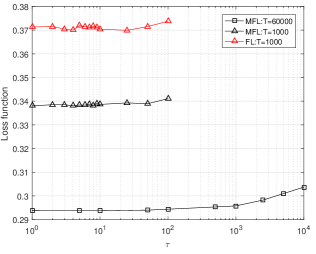
Figure 7: Loss function values with τ𝜏\tau

VII-B Simulation Evaluation

In this subsection, we verify the convergence acceleration of MFL and explore the effects of γ𝛾\gamma and τ𝜏\tau on MFL convergence by simulation evaluations.

VII-B1 Convergence

In our first simulation, the models of SVM, linear regression and logistic regression are trained and we verify the convergence of MFL. We set aggregation frequency τ=4𝜏4\tau=4 and momentum attenuation factor γ=0.5𝛾0.5\gamma=0.5. MFL, FL and MGD are performed based on the three machine learning model. MGD is implemented based on the global dataset which is obtained by gathering the distributed data on all nodes. The global loss functions of this three solutions are defined based on the same global training and testing data.

The curves of loss function values and accuracy with iterative times are presented in Fig. 5. We can see that the loss function curves for all the learning models are gradually convergent with iterative times. Similarly, the test accuracy curves for SVM gradually rise until convergence with iterative times. Therefore, convergence of MFL is verified. We also see that the descent speeds of MFL loss function curves on three learning models are always faster than those of FL while the centralized MGD convergence speeds are fastest. So compared with FL, MFL provides a significant improvement on convergence rate. MGD converges with the fastest speed because MFL and FL suffer the delay in global gradient update for τ=4𝜏4\tau=4.

Because linear and logistic regression can not provide the testing accuracy curves, we focus on the SVM model in the following experiments and further explore the impact of MFL parameters on convergence rate.

VII-B2 Effect of γ𝛾\gamma

We evaluate the impact of γ𝛾\gamma on the convergence rate of loss function. In this simulation, we still set aggregation frequency τ=4𝜏4\tau=4.

The experimental results are shown in Fig. 6. Subfigure (a) and (b) show that how different values of γ𝛾\gamma affect the convergence curves of loss function and testing accuracy, respectively. We can see that if γ=0𝛾0\gamma=0, the loss function and accuracy curves of MFL overlap with the corresponding ones of FL because MFL is equivalent to FL for γ=0𝛾0\gamma=0. When γ𝛾\gamma increases from 0 to 0.9, we can see the convergence rates on both loss function curves and accuracy curves also gradually increase. Subfigure (c) shows the change of final loss function value (T=1000𝑇1000T=1000) with 0<γ<10𝛾10<\gamma<1. From this subfigure, we can find the final loss function values of MFL are always smaller than FL with 0<γ<10𝛾10<\gamma<1. Compared with FL, convergence performance of MFL is improved. This is because 2(1βη)cosθβηp2>121𝛽𝜂𝜃𝛽𝜂superscript𝑝21\frac{2(1-\beta\eta)\cos\theta}{\beta\eta p^{2}}>1 and according to Proposition 3, the accelerated convergence range of MFL is 0<γ<10𝛾10<\gamma<1. We can see that when 0<γ<0.950𝛾0.950<\gamma<0.95, the loss function values decrease monotonically with γ𝛾\gamma so the convergence rate of MFL increases with γ𝛾\gamma. While γ>0.95𝛾0.95\gamma>0.95, the loss function values of MFL start to increase with a gradual deterioration of MFL convergence performance, and in this situation, MFL can not remain convergence. If the γ𝛾\gamma values are chosen to be close to 1, best around 0.9, MFL reaches the optimal convergence rate.

VII-B3 Effect of τ𝜏\tau

Finally, we evaluate the effect of different τ𝜏\tau on loss function of MFL. We record the final loss function values with τ𝜏\tau based on the three cases of T=1,000𝑇1000T=1,000 for FL, T=1,000𝑇1000T=1,000 for MFL and T=60,000𝑇60000T=60,000 for MFL. We set γ=0.5𝛾0.5\gamma=0.5 for MFL. The curves for the three cases are presented in Fig. 7. Comparing FL with MFL for T=1,000𝑇1000T=1,000, we see that the final loss function values of MFL are smaller than those of FL for any τ𝜏\tau. As declared in Proposition 3, under a small magnitude of T𝑇T and η=0.002𝜂0.002\eta=0.002 which is close to 0, MFL always converges much faster than FL. Further, for T=1,000𝑇1000T=1,000, the effect of τ𝜏\tau on convergence is slight because the curves of FL and MFL are relatively plain. This can be explained by Lemma 3, where 12ηφT12𝜂𝜑𝑇\frac{1}{2\eta\varphi T} and 12ωαT12𝜔𝛼𝑇\frac{1}{2\omega\alpha T} dominate the convergence upper-bound when the magnitude of T𝑇T is small. While T=60,000𝑇60000T=60,000, change of τ𝜏\tau affects convergence significantly and the final loss function values gradually increase with τ𝜏\tau. As the cases of T=1,000𝑇1000T=1,000 for MFL and FL, the case of T=60,000𝑇60000T=60,000 for MFL has a slight effect on convergence if τ<100𝜏100\tau<100. But if τ>100𝜏100\tau>100, MFL convergence performance is getting worse with τ𝜏\tau. According to the above analysis of τ𝜏\tau, setting an appropriate aggregation frequency will reduce convergence performance slightly with a decline of communication cost (in our cases, τ=100𝜏100\tau=100).

VIII Conclusion

In this paper, we have proposed MFL which performs MGD in local update step to solve the distributed machine learning problem. Firstly, we have established global convergence properties of MFL and derived an upper bound on MFL convergence rate. This theoretical upper bound shows that the sequence generated by MFL linearly converges to the global optimum point under certain conditions. Then, compared with FL, MFL provides accelerated convergence performance under the given conditions as presented in Proposition 3. Finally, based on MNIST dataset, our simulation results have verified the MFL convergence and confirmed the accelerated convergence of MFL.

References

  • [1] Chenyi Chen, Ari Seff, Alain Kornhauser, and Jianxiong Xiao. Deepdriving: Learning affordance for direct perception in autonomous driving. In Proc. ICCV, pages 2722–2730, 2015.
  • [2] Li Deng, Jinyu Li, Jui-Ting Huang, Kaisheng Yao, Dong Yu, Frank Seide, Michael Seltzer, Geoff Zweig, Xiaodong He, Jason Williams, et al. Recent advances in deep learning for speech research at microsoft. In Proc. ICASSP, pages 8604–8608. IEEE, 2013.
  • [3] Alex Krizhevsky, Ilya Sutskever, and Geoffrey E Hinton. Imagenet classification with deep convolutional neural networks. In Proc. NIPS, pages 1097–1105, 2012.
  • [4] Andre Esteva, Brett Kuprel, Roberto A Novoa, Justin Ko, Susan M Swetter, Helen M Blau, and Sebastian Thrun. Dermatologist-level classification of skin cancer with deep neural networks. Nature, 542(7639):115, 2017.
  • [5] Michael I Jordan and Tom M Mitchell. Machine learning: Trends, perspectives, and prospects. Science, 349(6245):255–260, 2015.
  • [6] Ramanan Subramanian and Faramarz Fekri. Sleep scheduling and lifetime maximization in sensor networks: fundamental limits and optimal solutions. In Proc. International Conf. Inf. Process. Sensor Netw., pages 218–225. IEEE, 2006.
  • [7] Gerhard P Fettweis. The tactile internet: Applications and challenges. IEEE Veh. Technol. Mag., 9(1):64–70, 2014.
  • [8] Milan Patel, Brian Naughton, Caroline Chan, Nurit Sprecher, Sadayuki Abeta, Adrian Neal, et al. Mobile-edge computing introductory technical white paper. White paper, mobile-edge computing (MEC) industry initiative, pages 1089–7801, 2014.
  • [9] Yuyi Mao, Changsheng You, Jun Zhang, Kaibin Huang, and Khaled B Letaief. A survey on mobile edge computing: The communication perspective. IEEE Commun. Surv. Tutorials, 19(4):2322–2358, 2017.
  • [10] Miao Hu, Lei Zhuang, Di Wu, Yipeng Zhou, Xu Chen, and Liang Xiao. Learning driven computation offloading for asymmetrically informed edge computing. IEEE Trans. Parallel Distrib. Syst., 2019.
  • [11] Xinhou Wang, Kezhi Wang, Song Wu, Sheng Di, Hai Jin, Kun Yang, and Shumao Ou. Dynamic resource scheduling in mobile edge cloud with cloud radio access network. IEEE Trans. Parallel Distrib. Syst., 29(11):2429–2445, 2018.
  • [12] Shuai Yu, Xin Wang, and Rami Langar. Computation offloading for mobile edge computing: A deep learning approach. In Proc. IEEE 28th Annu. Int. Sympo. Personal Indoor Mobile Radio Commun., pages 1–6. IEEE, 2017.
  • [13] Nguyen Quoc Viet Hung, Hoyoung Jeung, and Karl Aberer. An evaluation of model-based approaches to sensor data compression. IEEE Trans. Knowl. Data Eng., 25(11):2434–2447, 2012.
  • [14] Sheng Di, Dingwen Tao, Xin Liang, and Franck Cappello. Efficient lossy compression for scientific data based on pointwise relative error bound. IEEE Trans. Parallel Distrib. Syst., 30(2):331–345, 2018.
  • [15] Sheng Di and Franck Cappello. Optimization of error-bounded lossy compression for hard-to-compress hpc data. IEEE Trans. Parallel Distrib. Syst., 29(1):129–143, 2017.
  • [16] Gang Yang, Vincent YF Tan, Chin Keong Ho, See Ho Ting, and Yong Liang Guan. Wireless compressive sensing for energy harvesting sensor nodes. IEEE Trans. Signal Process., 61(18):4491–4505, 2013.
  • [17] Shancang Li, Li Da Xu, and Xinheng Wang. Compressed sensing signal and data acquisition in wireless sensor networks and internet of things. IEEE Trans. Ind. Inf., 9(4):2177–2186, 2012.
  • [18] Chenhan Xu, Kun Wang, Peng Li, Song Guo, Jiangtao Luo, Baoliu Ye, and Minyi Guo. Making big data open in edges: A resource-efficient blockchain-based approach. IEEE Trans. Parallel Distrib. Syst., 30(4):870–882, 2018.
  • [19] H Brendan McMahan, Eider Moore, Daniel Ramage, Seth Hampson, et al. Communication-efficient learning of deep networks from decentralized data. arXiv preprint arXiv:1602.05629, 2016.
  • [20] Shiqiang Wang, Tiffany Tuor, Theodoros Salonidis, Kin K Leung, Christian Makaya, Ting He, and Kevin Chan. When edge meets learning: Adaptive control for resource-constrained distributed machine learning. In Proc. IEEE INFOCOM, pages 63–71. IEEE, 2018.
  • [21] Shiqiang Wang, Tiffany Tuor, Theodoros Salonidis, Kin K Leung, Christian Makaya, Ting He, and Kevin Chan. Adaptive federated learning in resource constrained edge computing systems. IEEE J. Sel. Areas Commun., 37(6):1205–1221, 2019.
  • [22] Jakub Konečnỳ, H Brendan McMahan, Felix X Yu, Peter Richtárik, Ananda Theertha Suresh, and Dave Bacon. Federated learning: Strategies for improving communication efficiency. arXiv preprint arXiv:1610.05492, 2016.
  • [23] Corentin Hardy, Erwan Le Merrer, and Bruno Sericola. Distributed deep learning on edge-devices: feasibility via adaptive compression. In 16 th IEEE International Symposium on Network Computing and Applications (NCA), pages 1–8. IEEE, 2017.
  • [24] Keith Bonawitz, Vladimir Ivanov, Ben Kreuter, Antonio Marcedone, H Brendan McMahan, Sarvar Patel, Daniel Ramage, Aaron Segal, and Karn Seth. Practical secure aggregation for federated learning on user-held data. arXiv preprint arXiv:1611.04482, 2016.
  • [25] Keith Bonawitz, Vladimir Ivanov, Ben Kreuter, Antonio Marcedone, H Brendan McMahan, Sarvar Patel, Daniel Ramage, Aaron Segal, and Karn Seth. Practical secure aggregation for privacy-preserving machine learning. In Proc. ACM SIGSAC Conf. Comput. Commun. Secur. (CCS), pages 1175–1191. ACM, 2017.
  • [26] Takayuki Nishio and Ryo Yonetani. Client selection for federated learning with heterogeneous resources in mobile edge. arXiv preprint arXiv:1804.08333, 2018.
  • [27] Yue Zhao, Meng Li, Liangzhen Lai, Naveen Suda, Damon Civin, and Vikas Chandra. Federated learning with non-iid data. arXiv preprint arXiv:1806.00582, 2018.
  • [28] Arkadii Semenovich Nemirovsky and David Borisovich Yudin. Problem complexity and method efficiency in optimization. 1983.
  • [29] Boris T Polyak. Some methods of speeding up the convergence of iteration methods. USSR Comput. Math. Math. Phys., 4(5):1–17, 1964.
  • [30] Euhanna Ghadimi, Hamid Reza Feyzmahdavian, and Mikael Johansson. Global convergence of the heavy-ball method for convex optimization. In 2015 European Control Conf., pages 310–315. IEEE, 2015.
  • [31] Ning Qian. On the momentum term in gradient descent learning algorithms. Neural Netw., 12(1):145–151, 1999.
  • [32] Yurii Nesterov. Lectures on convex optimization, volume 137. Springer, 2018.
  • [33] Shai Shalev-Shwartz and Shai Ben-David. Understanding machine learning: From theory to algorithms. Cambridge university press, 2014.
  • [34] Sébastien Bubeck et al. Convex optimization: Algorithms and complexity. Found. and Trends in Mach. Learning, 8(3-4):231–357, 2015.

Appendix A MFL vs. Centralized MGD

Proposition 4.

When τ=1𝜏1\tau=1, MFL is equivalent to centralized MGD, i.e., the update rules of MFL yield the following equations:

d(t)d𝑡\displaystyle\textup{{d}}(t) =γd(t1)+F(w(t1))absent𝛾d𝑡1𝐹w𝑡1\displaystyle=\gamma\textup{{d}}(t-1)+\nabla F(\textup{{w}}(t-1))
w(t)w𝑡\displaystyle\textup{{w}}(t) =w(t1)ηd(t)absentw𝑡1𝜂d𝑡\displaystyle=\textup{{w}}(t-1)-\eta\textup{{d}}(t)
Proof.

When τ=1𝜏1\tau=1, according to the definition of MFL, we have d~i(t)=d(t)subscript~d𝑖𝑡d𝑡\widetilde{\textbf{d}}_{i}(t)=\textbf{d}(t) and w~i(t)=w(t)subscript~w𝑖𝑡w𝑡\widetilde{\textbf{w}}_{i}(t)=\textbf{w}(t) for node i𝑖i. Then

w(t)w𝑡\displaystyle\textbf{w}(t) =i=1N|𝒟i|wi(t)|𝒟|absentsuperscriptsubscript𝑖1𝑁subscript𝒟𝑖subscriptw𝑖𝑡𝒟\displaystyle=\frac{\sum_{i=1}^{N}|\mathcal{D}_{i}|\textbf{w}_{i}(t)}{|\mathcal{D}|}
=i=1N|𝒟i|(w~i(t1)ηdi(t))|𝒟|absentsuperscriptsubscript𝑖1𝑁subscript𝒟𝑖subscript~w𝑖𝑡1𝜂subscriptd𝑖𝑡𝒟\displaystyle=\frac{\sum_{i=1}^{N}|\mathcal{D}_{i}|(\widetilde{\textbf{w}}_{i}(t-1)-\eta\textbf{d}_{i}(t))}{|\mathcal{D}|}
=w(t1)ηi=1N|𝒟i|(γd~i(t1)+Fi(w~i(t1))|𝒟|\displaystyle=\textbf{w}(t-1)-\eta\frac{\sum_{i=1}^{N}|\mathcal{D}_{i}|(\gamma\widetilde{\textbf{d}}_{i}(t-1)+\nabla F_{i}(\widetilde{\textbf{w}}_{i}(t-1))}{|\mathcal{D}|}
=w(t1)ηγd(t1)ηi=1N|𝒟i|Fi(w(t1))|𝒟|absentw𝑡1𝜂𝛾d𝑡1𝜂superscriptsubscript𝑖1𝑁subscript𝒟𝑖subscript𝐹𝑖w𝑡1𝒟\displaystyle=\textbf{w}(t-1)-\eta\gamma\textbf{d}(t-1)-\eta\frac{\sum_{i=1}^{N}|\mathcal{D}_{i}|\nabla F_{i}(\textbf{w}(t-1))}{|\mathcal{D}|}
=w(t1)ηγd(t1)ηF(w(t1))absentw𝑡1𝜂𝛾d𝑡1𝜂𝐹w𝑡1\displaystyle=\textbf{w}(t-1)-\eta\gamma\textbf{d}(t-1)-\eta\nabla F(\textbf{w}(t-1))

where the last equality is derived because

i=1N|𝒟i|Fi(w)|𝒟|=(i=1N|𝒟i|Fi(w)|𝒟|)=F(w)superscriptsubscript𝑖1𝑁subscript𝒟𝑖subscript𝐹𝑖w𝒟superscriptsubscript𝑖1𝑁subscript𝒟𝑖subscript𝐹𝑖w𝒟𝐹w\displaystyle\frac{\sum_{i=1}^{N}|\mathcal{D}_{i}|\nabla F_{i}(\textbf{w})}{|\mathcal{D}|}=\nabla\left(\frac{\sum_{i=1}^{N}|\mathcal{D}_{i}|F_{i}(\textbf{w})}{|\mathcal{D}|}\right)=\nabla F(\textbf{w})

from the linearity of the gradient operator. So we can get

d(t)d𝑡\displaystyle\textbf{d}(t) =γd(t1)F(w(t1))absent𝛾d𝑡1𝐹w𝑡1\displaystyle=\gamma\textbf{d}(t-1)-\nabla F(\textbf{w}(t-1))
w(t)w𝑡\displaystyle\textbf{w}(t) =w(t1)ηd(t)absentw𝑡1𝜂d𝑡\displaystyle=\textbf{w}(t-1)-\eta\textbf{d}(t)

finally. ∎

Appendix B Proof of Proposition 1

We first introduce a lemma about sequence for the following proof preparation. The following lemma 4 provides the general formulas which can be used to match the inequality in Lemma 5.

Lemma 4.

Given

at=δiβ(1+ηβγBABAt1+ηβγAABBt)subscript𝑎𝑡subscript𝛿𝑖𝛽1𝜂𝛽𝛾𝐵𝐴𝐵superscript𝐴𝑡1𝜂𝛽𝛾𝐴𝐴𝐵superscript𝐵𝑡\displaystyle a_{t}=\frac{\delta_{i}}{\beta}\left(\frac{\frac{1+\eta\beta}{\gamma}-B}{A-B}A^{t}-\frac{\frac{1+\eta\beta}{\gamma}-A}{A-B}B^{t}\right) (24)
A+B=1+γ+ηβγ𝐴𝐵1𝛾𝜂𝛽𝛾\displaystyle A+B=\frac{1+\gamma+\eta\beta}{\gamma} (25)
AB=1γ𝐴𝐵1𝛾\displaystyle AB=\frac{1}{\gamma} (26)

where t=0,1,2,,0<γ<1,ηβ>0formulae-sequenceformulae-sequence𝑡0120𝛾1𝜂𝛽0t=0,1,2,...,0<\gamma<1,\eta\beta>0, we have

at1+ηβi=0t1ai=γat.subscript𝑎𝑡1𝜂𝛽superscriptsubscript𝑖0𝑡1subscript𝑎𝑖𝛾subscript𝑎𝑡\displaystyle a_{t-1}+\eta\beta\sum_{i=0}^{t-1}a_{i}=\gamma a_{t}. (27)
Proof.

For convenience, we define C1+ηβγBAB=A1AB𝐶1𝜂𝛽𝛾𝐵𝐴𝐵𝐴1𝐴𝐵C\triangleq\frac{\frac{1+\eta\beta}{\gamma}-B}{A-B}=\frac{A-1}{A-B} and DA1+ηβγAB=1BAB𝐷𝐴1𝜂𝛽𝛾𝐴𝐵1𝐵𝐴𝐵D\triangleq\frac{A-\frac{1+\eta\beta}{\gamma}}{A-B}=\frac{1-B}{A-B}. So at=δiβ(CAt+DBt)subscript𝑎𝑡subscript𝛿𝑖𝛽𝐶superscript𝐴𝑡𝐷superscript𝐵𝑡a_{t}=\frac{\delta_{i}}{\beta}(CA^{t}+DB^{t}). After eliminating B or A by (25) and (26), we get

γx2(1+γ+ηβ)x+1=0.𝛾superscript𝑥21𝛾𝜂𝛽𝑥10\displaystyle\gamma x^{2}-(1+\gamma+\eta\beta)x+1=0. (28)

Because ηβ>0𝜂𝛽0\eta\beta>0, we always have Δ=(1+γ+ηβ)24γ>0Δsuperscript1𝛾𝜂𝛽24𝛾0\Delta=(1+\gamma+\eta\beta)^{2}-4\gamma>0. Thus A𝐴A and B𝐵B can be derived as follows:

A𝐴\displaystyle A =(1+γ+ηβ)+(1+γ+ηβ)24γ2γabsent1𝛾𝜂𝛽superscript1𝛾𝜂𝛽24𝛾2𝛾\displaystyle=\frac{(1\!+\!\gamma+\!\eta\beta)\!+\!\sqrt{(1\!+\!\gamma\!+\!\eta\beta)^{2}\!-\!4\gamma}}{2\gamma} (29)
B𝐵\displaystyle B =(1+γ+ηβ)(1+γ+ηβ)24γ2γ.absent1𝛾𝜂𝛽superscript1𝛾𝜂𝛽24𝛾2𝛾\displaystyle=\frac{(1\!+\!\gamma+\!\eta\beta)\!-\!\sqrt{(1\!+\!\gamma\!+\!\eta\beta)^{2}\!-\!4\gamma}}{2\gamma}. (30)

Then we have

at1+ηβi=0t1aiγatsubscript𝑎𝑡1𝜂𝛽superscriptsubscript𝑖0𝑡1subscript𝑎𝑖𝛾subscript𝑎𝑡\displaystyle a_{t-1}+\eta\beta\sum_{i=0}^{t-1}a_{i}-\gamma a_{t}
=\displaystyle= δiβ(CAt1+DBt1)+ηβδiβCAt1A1subscript𝛿𝑖𝛽𝐶superscript𝐴𝑡1𝐷superscript𝐵𝑡1𝜂𝛽subscript𝛿𝑖𝛽𝐶superscript𝐴𝑡1𝐴1\displaystyle\frac{\delta_{i}}{\beta}\left(CA^{t-1}+DB^{t-1}\right)+\eta\beta\frac{\delta_{i}}{\beta}C\frac{A^{t}-1}{A-1}
+ηβδiβDBt1B1γδiβCAtγδiβDBt𝜂𝛽subscript𝛿𝑖𝛽𝐷superscript𝐵𝑡1𝐵1𝛾subscript𝛿𝑖𝛽𝐶superscript𝐴𝑡𝛾subscript𝛿𝑖𝛽𝐷superscript𝐵𝑡\displaystyle+\eta\beta\frac{\delta_{i}}{\beta}D\frac{B^{t}-1}{B-1}-\gamma\frac{\delta_{i}}{\beta}CA^{t}-\gamma\frac{\delta_{i}}{\beta}DB^{t}
=\displaystyle= δiβ[At1C1A(γA2(1+γ+ηβ)A+1)\displaystyle\frac{\delta_{i}}{\beta}\left[\frac{A^{t-1}C}{1-A}(\gamma A^{2}-(1+\gamma+\eta\beta)A+1)\right.
+Bt1D1B(γB2(1+γ+ηβ)B+1)ηβ(CA1+DB1)]\displaystyle\left.+\frac{B^{t-1}D}{1-B}(\gamma B^{2}\!-\!(1\!+\!\gamma\!+\!\eta\beta)B\!+\!1)\!-\!\eta\beta\left(\frac{C}{A-1}\!+\!\frac{D}{B-1}\right)\right]
=\displaystyle= ηδi(CA1+DB1)𝜂subscript𝛿𝑖𝐶𝐴1𝐷𝐵1\displaystyle-\eta\delta_{i}\left(\frac{C}{A-1}+\frac{D}{B-1}\right)
(because A𝐴A, B𝐵B satisfy (28))
=\displaystyle= 0.0\displaystyle 0.

So Lemma 4 has been proven. ∎

Then we study the difference between w~i(t)subscript~w𝑖𝑡\widetilde{\textbf{w}}_{i}(t) and w[k](t)subscriptwdelimited-[]𝑘𝑡\textbf{w}_{[k]}(t) for node i𝑖i. We obtain the following lemma.

Lemma 5.

For any interval [k]delimited-[]𝑘[k] with t[(k1)τ,kτ)𝑡𝑘1𝜏𝑘𝜏t\in[(k-1)\tau,k\tau), we have

w~i(t)w[k](t)fi(t(k1)τ)normsubscript~w𝑖𝑡subscriptwdelimited-[]𝑘𝑡subscript𝑓𝑖𝑡𝑘1𝜏\displaystyle\|\widetilde{\textup{{w}}}_{i}(t)-\textup{{w}}_{[k]}(t)\|\leq f_{i}(t-(k-1)\tau)

where we define the function fi(t)subscript𝑓𝑖𝑡f_{i}(t) as

fi(t)δiβ(γt(CAt+DBt)1).subscript𝑓𝑖𝑡subscript𝛿𝑖𝛽superscript𝛾𝑡𝐶superscript𝐴𝑡𝐷superscript𝐵𝑡1\displaystyle f_{i}(t)\triangleq\frac{\delta_{i}}{\beta}\left(\gamma^{t}(CA^{t}+DB^{t}\right)-1).
Proof.

When t=(k1)τ𝑡𝑘1𝜏t=(k-1)\tau, we know that

w~i((k1)τ)=w((k1)τ)=w[k]((k1)τ)subscript~w𝑖𝑘1𝜏w𝑘1𝜏subscriptwdelimited-[]𝑘𝑘1𝜏\widetilde{\textbf{w}}_{i}((k-1)\tau)=\textbf{w}((k-1)\tau)=\textbf{w}_{[k]}((k-1)\tau)

by the definition of w[k](t)subscriptwdelimited-[]𝑘𝑡\textbf{w}_{[k]}(t), and we get w~i(t)w[k](t)=0normsubscript~w𝑖𝑡subscriptwdelimited-[]𝑘𝑡0\|\widetilde{\textbf{w}}_{i}(t)-\textbf{w}_{[k]}(t)\|=0. While t=0𝑡0t=0, we can get fi(0)=0subscript𝑓𝑖00f_{i}(0)=0 easily. Hence, when t=(k1)τ𝑡𝑘1𝜏t=(k-1)\tau, Lemma 5 holds.

Firstly, we derive the upper bound of d~i(t)d[k](t)normsubscript~d𝑖𝑡subscriptddelimited-[]𝑘𝑡\|\widetilde{\textbf{d}}_{i}(t)-\textbf{d}_{[k]}(t)\| as follows. For t((k1)τ,kτ]𝑡𝑘1𝜏𝑘𝜏t\in((k-1)\tau,k\tau],

d~i(t)d[k](t)normsubscript~d𝑖𝑡subscriptddelimited-[]𝑘𝑡\displaystyle\|\widetilde{\textbf{d}}_{i}(t)-\textbf{d}_{[k]}(t)\|
=γd~i(t1)+Fi(w~i(t1))(γd[k](t1)+F(w[k](t1)))absentnorm𝛾subscript~d𝑖𝑡1subscript𝐹𝑖subscript~w𝑖𝑡1𝛾subscriptddelimited-[]𝑘𝑡1𝐹subscriptwdelimited-[]𝑘𝑡1\displaystyle\!=\!\|\!\gamma\!\widetilde{\textbf{d}}_{i}(t\!-\!1)\!+\!\nabla\!F_{i}(\widetilde{\textbf{w}}_{i}(t\!-\!1))\!-\!(\!\gamma\!\textbf{d}_{[k]}(t\!-\!1)+\nabla F(\textbf{w}_{[k]}(t\!-\!1\!)\!)\!)\!\|
(from (6) and (13))
Fi(w~i(t1))Fi(w[k](t1))\displaystyle\leq\!\|\nabla F_{i}(\widetilde{\textbf{w}}_{i}(t\!-\!1))\!-\!\nabla F_{i}(\textbf{w}_{[k]}(t\!-\!1))
+Fi(w[k](t1))F(w[k](t1))+γd~i(t1)d[k](t1)\displaystyle\!+\!\nabla F_{i}(\textbf{w}_{[k]}(t\!-\!1))\!-\!\nabla F(\textbf{w}_{[k]}(t\!-\!1))\|\!+\!\gamma\!\|\!\widetilde{\textbf{d}}_{i}(t\!-\!1)\!-\!\textbf{d}_{[k]}(t\!-\!1)\!\|
(from triangle inequality and adding a zero term)
βw~i(t1)w[k](t1)+δi+γd~i(t1)d[k](t1).absent𝛽normsubscript~w𝑖𝑡1subscriptwdelimited-[]𝑘𝑡1subscript𝛿𝑖𝛾normsubscript~d𝑖𝑡1subscriptddelimited-[]𝑘𝑡1\displaystyle\leq\beta\|\widetilde{\textbf{w}}_{i}(\!t\!-\!1)-\textbf{w}_{[k]}(t\!-\!1)\|\!+\!\delta_{i}+\gamma\|\widetilde{\textbf{d}}_{i}(t-1)-\textbf{d}_{[k]}(t-1)\|. (31)
(from the β𝛽\beta-smoothness and (11))

We present (B) for t,t1,,1+(k1)τ𝑡𝑡11𝑘1𝜏t,t-1,...,1+(k-1)\tau with multiplying 1,γ,,γt(k1)τ11𝛾superscript𝛾𝑡𝑘1𝜏11,\gamma,...,\gamma^{t-(k-1)\tau-1} respectively as the following:

d~i(t)d[k](t)βw~i(t1)w[k](t1)+δinormsubscript~d𝑖𝑡subscriptddelimited-[]𝑘𝑡𝛽normsubscript~w𝑖𝑡1subscriptwdelimited-[]𝑘𝑡1subscript𝛿𝑖\displaystyle\|\widetilde{\textbf{d}}_{i}(t)\!-\!\textbf{d}_{[k]}(t)\|\!\leq\!\beta\|\widetilde{\textbf{w}}_{i}(t\!-\!1)\!-\!\textbf{w}_{[k]}(t\!-\!1)\|\!+\!\delta_{i}
+γd~i(t1)d[k](t1)𝛾normsubscript~d𝑖𝑡1subscriptddelimited-[]𝑘𝑡1\displaystyle\!+\!\gamma\|\widetilde{\textbf{d}}_{i}(t-1)\!-\!\textbf{d}_{[k]}(t-1)\|
γd~i(t1)d[k](t1)γ(βw~i(t2)w[k](t2)+δi\displaystyle\gamma\|\widetilde{\textbf{d}}_{i}(t-1)\!-\!\textbf{d}_{[k]}(t-1)\|\leq\gamma(\beta\|\widetilde{\textbf{w}}_{i}(t-2)\!-\!\textbf{w}_{[k]}(t\!-\!2)\|\!+\!\delta_{i}
+γd~i(t2)d[k](t2))\displaystyle\!+\!\gamma\|\widetilde{\textbf{d}}_{i}(t\!-\!2)\!-\!\textbf{d}_{[k]}(t\!-\!2)\|)
\displaystyle...
γt(k1)τ1d~i(1+(k1)τ)d[k](1+(k1)τ)superscript𝛾𝑡𝑘1𝜏1normsubscript~d𝑖1𝑘1𝜏subscriptddelimited-[]𝑘1𝑘1𝜏\displaystyle\gamma^{t-(k-1)\tau-1}\|\widetilde{\textbf{d}}_{i}(1+(k-1)\tau)-\textbf{d}_{[k]}(1+(k-1)\tau)\|
γt(k1)τ1(βw~i((k1)τ)w[k]((k1)τ)\displaystyle\leq\gamma^{t-(k-1)\tau-1}(\beta\|\widetilde{\textbf{w}}_{i}((k-1)\tau)-\textbf{w}_{[k]}((k-1)\tau)\|
+δi+γd~i((k1)τ)d[k]((k1)τ)).\displaystyle+\delta_{i}+\gamma\|\widetilde{\textbf{d}}_{i}((k-1)\tau)-\textbf{d}_{[k]}((k-1)\tau)\|).

We define Gi(t)w~i(t)w[k](t)subscript𝐺𝑖𝑡normsubscript~w𝑖𝑡subscriptwdelimited-[]𝑘𝑡G_{i}(t)\triangleq\|\widetilde{\textbf{w}}_{i}(t)-\textbf{w}_{[k]}(t)\| for convenience. Accumulating all of the above inequalities, we have

d~i(t)d[k](t)β(Gi(t1)+γGi(t2)+γ2Gi(t3)\displaystyle\|\widetilde{\textbf{d}}_{i}(t)-\textbf{d}_{[k]}(t)\|\leq\beta(G_{i}(t-1)+\gamma G_{i}(t-2)+\gamma^{2}G_{i}(t-3)
++γt(k1)τ1Gi((k1)τ)+δi(1+γ+γ2++γt(k1)τ1)superscript𝛾𝑡𝑘1𝜏1subscript𝐺𝑖𝑘1𝜏subscript𝛿𝑖1𝛾superscript𝛾2superscript𝛾𝑡𝑘1𝜏1\displaystyle\!+\!...\!+\!\gamma^{t\!-(k\!-\!1)\tau\!-\!1}G_{i}((k\!-\!1)\tau)+\delta_{i}(1\!+\!\gamma\!+\!\gamma^{2}\!+\!...\!+\!\gamma^{t\!-\!(k\!-\!1)\tau\!-\!1})
+γt(k1)τd~i((k1)τ)d[k]((k1)τ).superscript𝛾𝑡𝑘1𝜏normsubscript~d𝑖𝑘1𝜏subscriptddelimited-[]𝑘𝑘1𝜏\displaystyle+\gamma^{t-(k-1)\tau}\|\widetilde{\textbf{d}}_{i}((k-1)\tau)-\textbf{d}_{[k]}((k-1)\tau)\|.

When t=(k1)τ𝑡𝑘1𝜏t=(k-1)\tau, d[k]((k1)=d((k1)τ)\textbf{d}_{[k]}((k-1)=\textbf{d}((k-1)\tau) according to the definition and d~i((k1)τ)=d((k1)τ)subscript~d𝑖𝑘1𝜏d𝑘1𝜏\widetilde{\textbf{d}}_{i}((k-1)\tau)=\textbf{d}((k-1)\tau) by the aggregation rules. So d~i((k1)τ)d[k]((k1)τ)=0normsubscript~d𝑖𝑘1𝜏subscriptddelimited-[]𝑘𝑘1𝜏0\|\widetilde{\textbf{d}}_{i}((k-1)\tau)-\textbf{d}_{[k]}((k-1)\tau)\|=0 and the above inequality can be further expressed as

d~i(t)d[k](t)β(Gi(t1)+γGi(t2)+γ2Gi(t3)\displaystyle\|\widetilde{\textbf{d}}_{i}(t)\!-\!\textbf{d}_{[k]}(t)\|\leq\beta(G_{i}(t\!-\!1)\!+\!\gamma G_{i}(t\!-\!2)+\gamma^{2}G_{i}(t\!-\!3)
++γt(k1)τ1Gi((k1)τ)+δi(1+γ+γ2++γt(k1)τ1).superscript𝛾𝑡𝑘1𝜏1subscript𝐺𝑖𝑘1𝜏subscript𝛿𝑖1𝛾superscript𝛾2superscript𝛾𝑡𝑘1𝜏1\displaystyle\!+\!...\!+\!\gamma^{t\!-\!(k\!-\!1)\tau\!-\!1}G_{i}((k\!-\!1)\tau)\!+\!\delta_{i}(\!1\!+\!\gamma\!+\!\gamma^{2}\!+\!...\!+\!\gamma^{t\!-(k\!-\!1)\tau\!-\!1}). (32)

We now derive the closed-form expression of the gap between w~i(t)subscript~w𝑖𝑡\widetilde{\textbf{w}}_{i}(t) and w[k](t)subscriptwdelimited-[]𝑘𝑡\textbf{w}_{[k]}(t). For t((k1)τ,kτ]𝑡𝑘1𝜏𝑘𝜏t\in((k-1)\tau,k\tau], we have

w~i(t)w[k](t)normsubscript~w𝑖𝑡subscriptwdelimited-[]𝑘𝑡\displaystyle\|\widetilde{\textbf{w}}_{i}(t)-\textbf{w}_{[k]}(t)\|
=w~i(t1)ηd~i(t)(w[k](t1)ηd[k](t))absentnormsubscript~w𝑖𝑡1𝜂subscript~d𝑖𝑡subscriptwdelimited-[]𝑘𝑡1𝜂subscriptddelimited-[]𝑘𝑡\displaystyle=\|\widetilde{\textbf{w}}_{i}(t-1)-\eta\widetilde{\textbf{d}}_{i}(t)-(\textbf{w}_{[k]}(t-1)-\eta\textbf{d}_{[k]}(t))\|
(from (7) and (14))
w~i(t1)w[k](t1)+ηd~i(t)d[k](t).absentnormsubscript~w𝑖𝑡1subscriptwdelimited-[]𝑘𝑡1𝜂normsubscript~d𝑖𝑡subscriptddelimited-[]𝑘𝑡\displaystyle\leq\|\widetilde{\textbf{w}}_{i}(t-1)-\textbf{w}_{[k]}(t-1)\|+\eta\|\widetilde{\textbf{d}}_{i}(t)-\textbf{d}_{[k]}(t)\|. (33)
(from triangle inequality)

Substituting inequality (B) into (33) and using Gi(t)subscript𝐺𝑖𝑡G_{i}(t) to denote w~i(t)w[k](t)normsubscript~w𝑖𝑡subscriptwdelimited-[]𝑘𝑡\|\widetilde{\textbf{w}}_{i}(t)-\textbf{w}_{[k]}(t)\| for t,t1,,1+(k1)τ𝑡𝑡11𝑘1𝜏t,t-1,...,1+(k-1)\tau, we have

Gi(t)Gi(t1)+ηβ(Gi(t1)+γGi(t2)+γ2Gi(t3)+\displaystyle G_{i}(t)\!\leq\!G_{i}(t\!-\!1)\!+\!\eta\beta(G_{i}(t\!-\!1)\!+\!\gamma G_{i}(t\!-\!2)\!+\!\gamma^{2}G_{i}(t\!-\!3)\!+\!...\!
+γt(k1)τ1Gi((k1)τ))+ηδi(1+γ+γ2++γt(k1)τ1).\displaystyle\!+\!\gamma^{t\!-\!(k\!-\!1)\tau\!-\!1}G_{i}((k\!-\!1)\tau))\!+\!\eta\delta_{i}(1\!+\!\gamma\!+\!\gamma^{2}\!+\!...\!+\!\gamma^{t\!-\!(k\!-\!1)\tau\!-\!1}). (34)

We suppose that

gi(t)subscript𝑔𝑖𝑡\displaystyle g_{i}(t) =δiβ(CAt+DBt)absentsubscript𝛿𝑖𝛽𝐶superscript𝐴𝑡𝐷superscript𝐵𝑡\displaystyle=\frac{\delta_{i}}{\beta}(CA^{t}+DB^{t}) (35)
fi(t)subscript𝑓𝑖𝑡\displaystyle f_{i}(t) =γtgi(t)δiβabsentsuperscript𝛾𝑡subscript𝑔𝑖𝑡subscript𝛿𝑖𝛽\displaystyle=\gamma^{t}g_{i}(t)-\frac{\delta_{i}}{\beta} (36)

where A𝐴A and B𝐵B are expressed as (29) and (30) respectively, C=A1AB𝐶𝐴1𝐴𝐵C=\frac{A-1}{A-B} and D=1BAB.𝐷1𝐵𝐴𝐵D=\frac{1-B}{A-B}.

Next we use induction to prove that Gi(t)fi(t(k1)τ)subscript𝐺𝑖𝑡subscript𝑓𝑖𝑡𝑘1𝜏G_{i}(t)\leq f_{i}(t-(k-1)\tau) satisfies inequality (B) opportunely. For the induction, we assume that

Gi(p)fi(p(k1)τ)subscript𝐺𝑖𝑝subscript𝑓𝑖𝑝𝑘1𝜏\displaystyle G_{i}(p)\leq f_{i}(p-(k-1)\tau) (37)

for some p[(k1)τ,t1]𝑝𝑘1𝜏𝑡1p\in[(k-1)\tau,t-1]. Therefore, according to (B), we have

Gi(t)subscript𝐺𝑖𝑡\displaystyle G_{i}(t)
fi(t1(k1)τ)+ηβ(fi(t1(k1)τ))absentsubscript𝑓𝑖𝑡1𝑘1𝜏𝜂𝛽subscript𝑓𝑖𝑡1𝑘1𝜏\displaystyle\!\leq\!f_{i}(t\!-\!1\!-\!(k\!-\!1)\tau)\!+\!\eta\beta(f_{i}(t\!-\!1\!-\!(k\!-\!1)\tau))
+γfi(t2(k1)τ)+γ2fi(t3(k1)τ)+𝛾subscript𝑓𝑖𝑡2𝑘1𝜏superscript𝛾2subscript𝑓𝑖𝑡3𝑘1𝜏\displaystyle+\gamma f_{i}(t\!-\!2\!-\!(k\!-\!1)\tau)\!+\!\gamma^{2}f_{i}(t\!-\!3\!-\!(k\!-\!1)\tau)\!+\!...\!
+γt(k1)τ1fi(0))+ηδi(1+γ+γ2++γt(k1)τ1)\displaystyle+\!\gamma^{t\!-\!(k\!-\!1)\tau\!-\!1}f_{i}(0))\!+\!\eta\delta_{i}(1\!+\!\gamma\!+\!\gamma^{2}\!+\!...\!+\!\gamma^{t\!-\!(k-\!1)\tau\!-1})
(from the induction assumption in (37))
=γt1(k1)τgi(t1(k1)τ)δiβabsentsuperscript𝛾𝑡1𝑘1𝜏subscript𝑔𝑖𝑡1𝑘1𝜏subscript𝛿𝑖𝛽\displaystyle=\gamma^{t-1-(k-1)\tau}g_{i}(t\!-\!1\!-\!(k\!-\!1)\tau)\!-\!\frac{\delta_{i}}{\beta}
+ηβγt1(k1)τ(gi(t1(k1)τ)+gi(t2(k1)τ)\displaystyle+\eta\beta\gamma^{t-1-(k-1)\tau}(g_{i}(t\!-\!1\!-\!(k\!-\!1)\tau)+g_{i}(t\!-\!2\!-\!(k\!-\!1)\tau)
+gi(t3(k1)τ)++gi(0))\displaystyle+g_{i}(t\!-\!3\!-\!(k\!-\!1)\tau)\!+\!...\!+\!g_{i}(0))
(from (36))
=γt(k1)τgi(t(k1)τ)δiβabsentsuperscript𝛾𝑡𝑘1𝜏subscript𝑔𝑖𝑡𝑘1𝜏subscript𝛿𝑖𝛽\displaystyle=\gamma^{t-(k-1)\tau}g_{i}(t-(k-1)\tau)-\frac{\delta_{i}}{\beta}
(from Lemma 4 and gi(t)=atsubscript𝑔𝑖𝑡subscript𝑎𝑡g_{i}(t)=a_{t})
=fi(t(k1)τ).absentsubscript𝑓𝑖𝑡𝑘1𝜏\displaystyle=f_{i}(t-(k-1)\tau).

Using the induction, we have proven that w~i(t)w[k](t)fi(t(k1)τ)normsubscript~w𝑖𝑡subscriptwdelimited-[]𝑘𝑡subscript𝑓𝑖𝑡𝑘1𝜏\|\widetilde{\textbf{w}}_{i}(t)-\textbf{w}_{[k]}(t)\|\leq f_{i}(t-(k-1)\tau) for all t[(k1)τ,kτ]𝑡𝑘1𝜏𝑘𝜏t\in[(k-1)\tau,k\tau]. ∎

Now, according to the result of lemma 5, we extend the difference from w~i(t)subscript~w𝑖𝑡\widetilde{\textbf{w}}_{i}(t) to the global one w(t)w𝑡\textbf{w}(t) to prove Proposition 1.

Proof of Proposition 1.

First of all, we derive the gap between d(t)d𝑡\textbf{d}(t) and d[k](t)subscriptddelimited-[]𝑘𝑡\textbf{d}_{[k]}(t). we define

p(t)γt(CAt+DBt)1.𝑝𝑡superscript𝛾𝑡𝐶superscript𝐴𝑡𝐷superscript𝐵𝑡1\displaystyle p(t)\triangleq\gamma^{t}(CA^{t}+DB^{t})-1. (38)

So we get

fi(t)=δiβp(t).subscript𝑓𝑖𝑡subscript𝛿𝑖𝛽𝑝𝑡\displaystyle f_{i}(t)=\frac{\delta_{i}}{\beta}p(t). (39)

From (6) and (8), we have

d(t)=γd(t1)i|𝒟i|Fi(w~i(t1))|𝒟|.d𝑡𝛾d𝑡1subscript𝑖subscript𝒟𝑖subscript𝐹𝑖subscript~w𝑖𝑡1𝒟\displaystyle\textbf{d}(t)=\gamma\textbf{d}(t-1)-\frac{\sum_{i}|\mathcal{D}_{i}|\nabla F_{i}(\widetilde{\textbf{w}}_{i}(t-1))}{|\mathcal{D}|}. (40)

For t((k1)τ,kτ]𝑡𝑘1𝜏𝑘𝜏t\in((k-1)\tau,k\tau], we have

d(t)d[k](t)normd𝑡subscriptddelimited-[]𝑘𝑡\displaystyle\|\textbf{d}(t)-\textbf{d}_{[k]}(t)\|
=γd(t1)i|𝒟i|Fi(w~i(t1))|𝒟|\displaystyle=\|\gamma\textbf{d}(t-1)-\frac{\sum_{i}|\mathcal{D}_{i}|\nabla F_{i}(\widetilde{\textbf{w}}_{i}(t-1))}{|\mathcal{D}|}
γd[k](t1)+F(w[k](t1))\displaystyle-\gamma\textbf{d}_{[k]}(t-1)+\nabla F(\textbf{w}_{[k]}(t-1))\|
(from (40) and (13))
γd(t1)d[k](t1)absent𝛾normd𝑡1subscriptddelimited-[]𝑘𝑡1\displaystyle\leq\gamma\|\textbf{d}(t-1)-\textbf{d}_{[k]}(t-1)\|
+(i|𝒟i|Fi(w~i(t1))Fi(w[k](t1))|𝒟|)subscript𝑖subscript𝒟𝑖normsubscript𝐹𝑖subscript~w𝑖𝑡1subscript𝐹𝑖subscriptwdelimited-[]𝑘𝑡1𝒟\displaystyle+\left(\frac{\sum_{i}|\mathcal{D}_{i}|\|\nabla F_{i}(\widetilde{\textbf{w}}_{i}(t-1))-\nabla F_{i}(\textbf{w}_{[k]}(t-1))\|}{|\mathcal{D}|}\right)
γd(t1)d[k](t1)+β(i|𝒟i|fi(t1(k1)τ)|𝒟|)absent𝛾normd𝑡1subscriptddelimited-[]𝑘𝑡1𝛽subscript𝑖subscript𝒟𝑖subscript𝑓𝑖𝑡1𝑘1𝜏𝒟\displaystyle\!\leq\gamma\|\textbf{d}(t-1)-\textbf{d}_{[k]}(t-1)\|+\!\beta\!\left(\frac{\sum_{i}|\mathcal{D}_{i}|f_{i}(t\!-\!1\!-\!(k\!-\!1)\tau)}{|\mathcal{D}|}\!\right)
(from the β𝛽\beta-smoothness and Lemma 5)
=γd(t1)d[k](t1)+δp(t1(t1)τ).absent𝛾normd𝑡1subscriptddelimited-[]𝑘𝑡1𝛿𝑝𝑡1𝑡1𝜏\displaystyle=\gamma\|\textbf{d}(t-1)-\textbf{d}_{[k]}(t-1)\|+\delta p(t-1-(t-1)\tau). (41)
(from (39) and (12))

We present (41) for t,t1,,1+(k1)τ𝑡𝑡11𝑘1𝜏t,t-1,...,1+(k-1)\tau with multiplying 1,γ,,γt1(k1)τ1𝛾superscript𝛾𝑡1𝑘1𝜏1,\gamma,...,\gamma^{t-1-(k-1)\tau} respectively as the following:

d(t)d[k](t)normd𝑡subscriptddelimited-[]𝑘𝑡\displaystyle\|\textbf{d}(t)-\textbf{d}_{[k]}(t)\|
γd(t1)d[k](t1)+δp(t1(t1)τ)absent𝛾normd𝑡1subscriptddelimited-[]𝑘𝑡1𝛿𝑝𝑡1𝑡1𝜏\displaystyle\leq\gamma\|\textbf{d}(t-1)-\textbf{d}_{[k]}(t-1)\|+\delta p(t-1-(t-1)\tau)
γd(t1)d[k](t1)𝛾normd𝑡1subscriptddelimited-[]𝑘𝑡1\displaystyle\gamma\|\textbf{d}(t-1)-\textbf{d}_{[k]}(t-1)\|
γ2d(t2)d[k](t2)+γδp(t2(t1)τ)absentsuperscript𝛾2normd𝑡2subscriptddelimited-[]𝑘𝑡2𝛾𝛿𝑝𝑡2𝑡1𝜏\displaystyle\leq\gamma^{2}\|\textbf{d}(t-2)-\textbf{d}_{[k]}(t-2)\|+\gamma\delta p(t-2-(t-1)\tau)
\displaystyle...
γt1(k1τ)d((k1)τ+1)d[k]((k1)τ)superscript𝛾𝑡1𝑘1𝜏normd𝑘1𝜏1subscriptddelimited-[]𝑘𝑘1𝜏\displaystyle\gamma^{t-1-(k-1\tau)}\|\textbf{d}((k-1)\tau+1)-\textbf{d}_{[k]}((k-1)\tau)\|
γt(k1)τd((k1)τ)d[k]((k1)τ)+γt(k1)τδp(0).absentsuperscript𝛾𝑡𝑘1𝜏normd𝑘1𝜏subscriptddelimited-[]𝑘𝑘1𝜏superscript𝛾𝑡𝑘1𝜏𝛿𝑝0\displaystyle\leq\gamma^{t-(k-1)\tau}\|\textbf{d}((k-1)\tau)\!-\!\textbf{d}_{[k]}((k-1)\tau)\|\!+\!\gamma^{t-(k-1)\tau}\delta p(0).

By summing up the left and right sides of the above inequalities respectively, we have

d(t)d[k](t)normd𝑡subscriptddelimited-[]𝑘𝑡\displaystyle\|\textbf{d}(t)-\textbf{d}_{[k]}(t)\|
δ(γt1(k1)τp(0)+\displaystyle\leq\delta(\gamma^{t-1-(k-1)\tau}p(0)+...
+γp(t2(k1)τ)+p(t1(k1)τ))\displaystyle+\gamma p(t-2-(k-1)\tau)+p(t-1-(k-1)\tau))
=δ[(C(γA)t0γ(A1)+D(γB)t0γ(B1))γt01γ1]absent𝛿delimited-[]𝐶superscript𝛾𝐴subscript𝑡0𝛾𝐴1𝐷superscript𝛾𝐵subscript𝑡0𝛾𝐵1superscript𝛾subscript𝑡01𝛾1\displaystyle=\delta\left[\left(\frac{C(\gamma A)^{t_{0}}}{\gamma(A-1)}+\frac{D(\gamma B)^{t_{0}}}{\gamma(B-1)}\right)-\frac{\gamma^{t_{0}}-1}{\gamma-1}\right] (42)

where t0=t(k1)τsubscript𝑡0𝑡𝑘1𝜏t_{0}=t-(k-1)\tau.

Then we can derive the upper bound between w(t)w𝑡\textbf{w}(t) and w[k](t)subscriptwdelimited-[]𝑘𝑡\textbf{w}_{[k]}(t) by (42). From (7), (8), (9) and (14), we have

w(t)w[k](t)normw𝑡subscriptwdelimited-[]𝑘𝑡\displaystyle\|\textbf{w}(t)-\textbf{w}_{[k]}(t)\|
=w(t1)ηd(t)w[k](t1)+ηd[k](t)absentnormw𝑡1𝜂d𝑡subscriptwdelimited-[]𝑘𝑡1𝜂subscriptddelimited-[]𝑘𝑡\displaystyle=\|\textbf{w}(t-1)-\eta\textbf{d}(t)-\textbf{w}_{[k]}(t-1)+\eta\textbf{d}_{[k]}(t)\|
w(t1)w[k](t1)+ηd(t)d[k](t).absentnormw𝑡1subscriptwdelimited-[]𝑘𝑡1𝜂normd𝑡subscriptddelimited-[]𝑘𝑡\displaystyle\leq\|\textbf{w}(t-1)-\textbf{w}_{[k]}(t-1)\|+\eta\|\textbf{d}(t)-\textbf{d}_{[k]}(t)\|.

According to (42),

w(t)w[k](t)w(t1)w[k](t1)normw𝑡subscriptwdelimited-[]𝑘𝑡normw𝑡1subscriptwdelimited-[]𝑘𝑡1\displaystyle\|\textbf{w}(t)-\textbf{w}_{[k]}(t)\|-\|\textbf{w}(t-1)-\textbf{w}_{[k]}(t-1)\|
ηδ[(C(γA)t0γ(A1)+D(γB)t0γ(B1))γt01γ1].absent𝜂𝛿delimited-[]𝐶superscript𝛾𝐴subscript𝑡0𝛾𝐴1𝐷superscript𝛾𝐵subscript𝑡0𝛾𝐵1superscript𝛾subscript𝑡01𝛾1\displaystyle\leq\eta\delta\left[\left(\frac{C(\gamma A)^{t_{0}}}{\gamma(A-1)}+\frac{D(\gamma B)^{t_{0}}}{\gamma(B-1)}\right)-\frac{\gamma^{t_{0}}-1}{\gamma-1}\right]. (43)

When t=(k1)τ𝑡𝑘1𝜏t=(k-1)\tau, we have w(t)w[k](t)=0normw𝑡subscriptwdelimited-[]𝑘𝑡0\|\textbf{w}(t)-\textbf{w}_{[k]}(t)\|=0 according to the definition. By summing up (42) over t((k1)τ,kτ]𝑡𝑘1𝜏𝑘𝜏t\in((k-1)\tau,k\tau], we have

w(t)w[k](t)normw𝑡subscriptwdelimited-[]𝑘𝑡\displaystyle\|\textbf{w}(t)-\textbf{w}_{[k]}(t)\|
i=1t0ηδ[(C(γA)iγ(A1)+D(γB)iγ(B1))γi1γ1]absentsuperscriptsubscript𝑖1subscript𝑡0𝜂𝛿delimited-[]𝐶superscript𝛾𝐴𝑖𝛾𝐴1𝐷superscript𝛾𝐵𝑖𝛾𝐵1superscript𝛾𝑖1𝛾1\displaystyle\leq\sum_{i=1}^{t_{0}}\eta\delta\left[\left(\frac{C(\gamma A)^{i}}{\gamma(A-1)}+\frac{D(\gamma B)^{i}}{\gamma(B-1)}\right)-\frac{\gamma^{i}-1}{\gamma-1}\right]
=ηδ[E((γA)t01)+F((γB)t01)γ(γt01)(γ1)t0(γ1)2]absent𝜂𝛿delimited-[]𝐸superscript𝛾𝐴subscript𝑡01𝐹superscript𝛾𝐵subscript𝑡01𝛾superscript𝛾subscript𝑡01𝛾1subscript𝑡0superscript𝛾12\displaystyle\!=\!\eta\delta\!\left[E((\gamma A)^{t_{0}}\!-\!1)\!+\!F((\gamma B)^{t_{0}}\!-\!1)\!-\!\frac{\gamma(\gamma^{t_{0}}\!-\!1)\!-\!(\gamma\!-\!1)t_{0}}{(\gamma-1)^{2}}\right]
=ηδ[E(γA)t0+F(γB)t01ηβγ(γt01)(γ1)t0(γ1)2]absent𝜂𝛿delimited-[]𝐸superscript𝛾𝐴subscript𝑡0𝐹superscript𝛾𝐵subscript𝑡01𝜂𝛽𝛾superscript𝛾subscript𝑡01𝛾1subscript𝑡0superscript𝛾12\displaystyle=\!\eta\delta\left[E(\gamma A)^{t_{0}}\!+\!F(\gamma B)^{t_{0}}\!-\!\frac{1}{\eta\beta}\!-\!\frac{\gamma(\gamma^{t_{0}}-1)-(\gamma-1)t_{0}}{(\gamma-1)^{2}}\right]
=h(t0)absentsubscript𝑡0\displaystyle=h(t_{0})

where E=A(AB)(γA1)𝐸𝐴𝐴𝐵𝛾𝐴1E=\frac{A}{(A-B)(\gamma A-1)}, F=B(AB)(1γB)𝐹𝐵𝐴𝐵1𝛾𝐵F=\frac{B}{(A-B)(1-\gamma B)} and t0=t(k1)τsubscript𝑡0𝑡𝑘1𝜏t_{0}=t-(k-1)\tau. The last equality is because E+F=1ηβ𝐸𝐹1𝜂𝛽E+F=\frac{1}{\eta\beta}.

Appendix C Proof of increasing of h(x)𝑥h(x)

Firstly, we introduce the following lemma.

Lemma 6.

Given A𝐴A, B𝐵B, C𝐶C and D𝐷D according to their definitions, then the following inequality

C(γA)i+D(γB)i(1+ηβ)i𝐶superscript𝛾𝐴𝑖𝐷superscript𝛾𝐵𝑖superscript1𝜂𝛽𝑖C(\gamma A)^{i}+D(\gamma B)^{i}\geq(1+\eta\beta)^{i}

holds for i=0,1,2,3,𝑖0123i=0,1,2,3,....

Proof.

Note that C+D=1𝐶𝐷1C+D=1 and C>0,D>0formulae-sequence𝐶0𝐷0C>0,D>0. When i=0𝑖0i=0, C(γA)i+D(γB)i=(1+ηβ)i=0𝐶superscript𝛾𝐴𝑖𝐷superscript𝛾𝐵𝑖superscript1𝜂𝛽𝑖0C(\gamma A)^{i}+D(\gamma B)^{i}=(1+\eta\beta)^{i}=0 and the inequality holds. When i=1𝑖1i=1,

C(γA)i+D(γB)i𝐶superscript𝛾𝐴𝑖𝐷superscript𝛾𝐵𝑖\displaystyle C(\gamma A)^{i}+D(\gamma B)^{i}
=\displaystyle= γ(CA+DB)𝛾𝐶𝐴𝐷𝐵\displaystyle\gamma(CA+DB)
=\displaystyle= γ(A1ABA+1BABB)𝛾𝐴1𝐴𝐵𝐴1𝐵𝐴𝐵𝐵\displaystyle\gamma\left(\frac{A-1}{A-B}A+\frac{1-B}{A-B}B\right)
(from the definition of C,D𝐶𝐷C,D)
=\displaystyle= γ(A+B1)𝛾𝐴𝐵1\displaystyle\gamma(A+B-1)
(from A+B=1+γ+ηβγ𝐴𝐵1𝛾𝜂𝛽𝛾A+B=\frac{1+\gamma+\eta\beta}{\gamma})
=\displaystyle= 1+ηβ.1𝜂𝛽\displaystyle 1+\eta\beta.

The equality still holds. When i>1𝑖1i>1(i𝑖i is an integer), according to Jensen’s inequality, we have

C(γA)i+D(γB)i𝐶superscript𝛾𝐴𝑖𝐷superscript𝛾𝐵𝑖\displaystyle C(\gamma A)^{i}+D(\gamma B)^{i}
>\displaystyle> (γCA+γDB)isuperscript𝛾𝐶𝐴𝛾𝐷𝐵𝑖\displaystyle(\gamma CA+\gamma DB)^{i}
(because f(x)=xi𝑓𝑥superscript𝑥𝑖f(x)=x^{i} is concave)
=\displaystyle= (1+ηβ)i.superscript1𝜂𝛽𝑖\displaystyle(1+\eta\beta)^{i}.
(from i=1𝑖1i=1)

In summary, we have proven the above lemma. ∎

Then we start to proof h(x)𝑥h(x) increases with x𝑥x.

Proof of increasing of h(x).

That h(x)𝑥h(x) increases with x𝑥x is equivalent to

h(x)h(x1)0𝑥𝑥10h(x)-h(x-1)\geq 0

for x1𝑥1x\geq 1 (x𝑥x is an integer). Considering x=0𝑥0x=0 or 1, we have

h(0)=ηδ(E+F1ηβ)=00𝜂𝛿𝐸𝐹1𝜂𝛽0\displaystyle h(0)=\eta\delta(E+F-\frac{1}{\eta\beta})=0 (44)
h(1)=ηδ[γ(EA+FB)1ηβ1]=0.1𝜂𝛿delimited-[]𝛾𝐸𝐴𝐹𝐵1𝜂𝛽10\displaystyle h(1)=\eta\delta\left[\gamma(EA+FB)-\frac{1}{\eta\beta}-1\right]=0. (45)
(because EA+FB=1+ηβγηβ𝐸𝐴𝐹𝐵1𝜂𝛽𝛾𝜂𝛽EA+FB=\frac{1+\eta\beta}{\gamma\eta\beta} which can be derived easily)

So when x=1𝑥1x=1, h(x)h(x1)=0𝑥𝑥10h(x)-h(x-1)=0.

When x>1𝑥1x>1, we first prove p(x)0𝑝𝑥0p(x)\geq 0 as follows. According to Lemma 6,

p(x)𝑝𝑥\displaystyle p(x) =C(γA)x+D(γB)x1absent𝐶superscript𝛾𝐴𝑥𝐷superscript𝛾𝐵𝑥1\displaystyle=C(\gamma A)^{x}+D(\gamma B)^{x}-1
(1+ηβ)x1absentsuperscript1𝜂𝛽𝑥1\displaystyle\geq(1+\eta\beta)^{x}-1
0.absent0\displaystyle\geq 0. (46)

Then we have

h(x)h(x1)𝑥𝑥1\displaystyle h(x)-h(x-1)
=ηδ[(C(γA)xγ(A1)+D(γB)xγ(B1))γx1γ1]absent𝜂𝛿delimited-[]𝐶superscript𝛾𝐴𝑥𝛾𝐴1𝐷superscript𝛾𝐵𝑥𝛾𝐵1superscript𝛾𝑥1𝛾1\displaystyle=\eta\delta\left[\left(\frac{C(\gamma A)^{x}}{\gamma(A-1)}+\frac{D(\gamma B)^{x}}{\gamma(B-1)}\right)-\frac{\gamma^{x}-1}{\gamma-1}\right]
=ηδ(γx1p(0)++γp(x2)+p(x1))absent𝜂𝛿superscript𝛾𝑥1𝑝0𝛾𝑝𝑥2𝑝𝑥1\displaystyle=\eta\delta(\gamma^{x-1}p(0)+...+\gamma p(x-2)+p(x-1))
(from (42) and x=t(k1)τ𝑥𝑡𝑘1𝜏x=t-(k-1)\tau)
0.absent0\displaystyle\geq 0.
(because γ>0𝛾0\gamma>0 and p(x)0𝑝𝑥0p(x)\geq 0 according to (46))

Therefore, h(x)𝑥h(x) increases with x𝑥x. ∎

Appendix D Proof of Lemma 2

Proof of Lemma 2.

To prove Lemma 2, we present some necessary definitions firstly.

Given 1kK1𝑘𝐾1\leq k\leq K where K=Tτ𝐾𝑇𝜏K=\frac{T}{\tau}, we define

c[k](t)F(w[k](t))F(w).subscript𝑐delimited-[]𝑘𝑡𝐹subscriptwdelimited-[]𝑘𝑡𝐹superscriptwc_{[k]}(t)\triangleq F(\textbf{w}_{[k]}(t))-F(\textbf{w}^{*}).

According to the lower bound of any gradient methods for a β𝛽\beta-smooth convex function from [34, Theorem 3.14], we have

c[k](t)>0subscript𝑐delimited-[]𝑘𝑡0c_{[k]}(t)>0

for any k𝑘k and t𝑡t. According to the definition of θ[k](t)subscript𝜃delimited-[]𝑘𝑡\theta_{[k]}(t), θ[k](t)subscript𝜃delimited-[]𝑘𝑡\theta_{[k]}(t) denotes the angle between vector F(w[k](t)\nabla F(\textbf{w}_{[k]}(t) and d[k](t)subscriptddelimited-[]𝑘𝑡\textbf{d}_{[k]}(t) so that

cosθ[k](t)=F(w[k](t))Td[k](t)F(w[k](t)d[k](t)\cos\theta_{[k]}(t)=\frac{\nabla F(\textbf{w}_{[k]}(t))^{\mathrm{T}}\textbf{d}_{[k]}(t)}{\|\nabla F(\textbf{w}_{[k]}(t)\|\|\textbf{d}_{[k]}(t)\|}

for t[k]𝑡delimited-[]𝑘t\in[k]. We assume cosθ[k](t)0subscript𝜃delimited-[]𝑘𝑡0\cos\theta_{[k]}(t)\geq 0 for 1kK1𝑘𝐾1\leq k\leq K with t[k]𝑡delimited-[]𝑘t\in[k] and define θ=max1kK,t[k]θ[k](t)𝜃subscriptformulae-sequence1𝑘𝐾𝑡delimited-[]𝑘subscript𝜃delimited-[]𝑘𝑡\theta=\max_{1\leq k\leq K,t\in[k]}\theta_{[k]}(t). From the definition of p𝑝p, we have

p=max1kK,t[k]d[k](t)F(w[k](t)).𝑝subscriptformulae-sequence1𝑘𝐾𝑡delimited-[]𝑘normsubscriptddelimited-[]𝑘𝑡norm𝐹subscriptwdelimited-[]𝑘𝑡p=\max_{1\leq k\leq K,t\in[k]}\frac{\|\textbf{d}_{[k]}(t)\|}{\|\nabla F(\textbf{w}_{[k]}(t))\|}.

Because condition 1 of Lemma 2 and Assumption 1, the sequence generated by MGD converges to the optimum point [29, Theorem 9].

Then we derive the upper bound of c[k](t+1)c[k](t)subscript𝑐delimited-[]𝑘𝑡1subscript𝑐delimited-[]𝑘𝑡c_{[k]}(t+1)-c_{[k]}(t).

Because F()𝐹F(\cdot) is β𝛽\beta-smooth, we have

F(x)F(y)F(y)T(xy)+β2xy2𝐹x𝐹y𝐹superscriptyTxy𝛽2superscriptnormxy2\displaystyle F(\textbf{x})-F(\textbf{y})\leq\nabla F(\textbf{y})^{\mathrm{T}}(\textbf{x}-\textbf{y})+\frac{\beta}{2}\|\textbf{x}-\textbf{y}\|^{2}

according to [34, Lemma 3.4]. Then,

c[k]subscript𝑐delimited-[]𝑘\displaystyle c_{[k]} (t+1)c[k](t)𝑡1subscript𝑐delimited-[]𝑘𝑡\displaystyle(t+1)-c_{[k]}(t)
=F(w[k](t+1))F(w[k](t))absent𝐹subscriptwdelimited-[]𝑘𝑡1𝐹subscriptwdelimited-[]𝑘𝑡\displaystyle=F(\textbf{w}_{[k]}(t+1))-F(\textbf{w}_{[k]}(t))
F(w[k](t))T(w[k](t+1)w[k](t))absent𝐹superscriptsubscriptwdelimited-[]𝑘𝑡Tsubscriptwdelimited-[]𝑘𝑡1subscriptwdelimited-[]𝑘𝑡\displaystyle\leq\nabla F(\textbf{w}_{[k]}(t))^{\mathrm{T}}(\textbf{w}_{[k]}(t+1)-\textbf{w}_{[k]}(t))
+β2w[k](t+1)w[k](t)2𝛽2superscriptnormsubscriptwdelimited-[]𝑘𝑡1subscriptwdelimited-[]𝑘𝑡2\displaystyle+\frac{\beta}{2}\|\textbf{w}_{[k]}(t+1)-\textbf{w}_{[k]}(t)\|^{2}
=ηF(w[k](t))Td[k](t+1)+βη22d[k](t+1)2absent𝜂𝐹superscriptsubscriptwdelimited-[]𝑘𝑡Tsubscriptddelimited-[]𝑘𝑡1𝛽superscript𝜂22superscriptnormsubscriptddelimited-[]𝑘𝑡12\displaystyle=-\eta\nabla F(\textbf{w}_{[k]}(t))^{\mathrm{T}}\textbf{d}_{[k]}(t+1)+\frac{\beta\eta^{2}}{2}\|\textbf{d}_{[k]}(t+1)\|^{2}
=ηF(w[k](t))T(γd[k](t)+F(w[k](t)))absent𝜂𝐹superscriptsubscriptwdelimited-[]𝑘𝑡T𝛾subscriptddelimited-[]𝑘𝑡𝐹subscriptwdelimited-[]𝑘𝑡\displaystyle=-\eta\nabla F(\textbf{w}_{[k]}(t))^{\mathrm{T}}(\gamma\textbf{d}_{[k]}(t)+\nabla F(\textbf{w}_{[k]}(t)))
+βη22γd[k](t)+F(w[k](t))2𝛽superscript𝜂22superscriptnorm𝛾subscriptddelimited-[]𝑘𝑡𝐹subscriptwdelimited-[]𝑘𝑡2\displaystyle+\frac{\beta\eta^{2}}{2}\|\gamma\textbf{d}_{[k]}(t)+\nabla F(\textbf{w}_{[k]}(t))\|^{2}
=η(1βη2)F(w[k](t))2+βη2γ22d[k](t)2absent𝜂1𝛽𝜂2superscriptnorm𝐹subscriptwdelimited-[]𝑘𝑡2𝛽superscript𝜂2superscript𝛾22superscriptnormsubscriptddelimited-[]𝑘𝑡2\displaystyle=-\eta(1-\frac{\beta\eta}{2})\|\nabla F(\textbf{w}_{[k]}(t))\|^{2}+\frac{\beta\eta^{2}\gamma^{2}}{2}\|\textbf{d}_{[k]}(t)\|^{2}
ηγ(1βη)F(w[k](t))Td[k](t)𝜂𝛾1𝛽𝜂𝐹superscriptsubscriptwdelimited-[]𝑘𝑡𝑇subscriptddelimited-[]𝑘𝑡\displaystyle-\eta\gamma(1-\beta\eta)\nabla F(\textbf{w}_{[k]}(t))^{T}\textbf{d}_{[k]}(t)
(η(1βη2)+βη2γ2p22\displaystyle\leq\!(-\!\eta(1\!-\!\frac{\beta\eta}{2})\!+\!\frac{\beta\eta^{2}\gamma^{2}p^{2}}{2}\!
ηγ(1βη)cosθ)F(w[k](t))2\displaystyle-\!\eta\gamma(1\!-\!\beta\eta)\cos\theta\!)\|\nabla F(\textbf{w}_{[k]}(t))\|\!^{2} (47)

where the second term in (D) is because

d[k](t)pF(w[k](t))normsubscriptddelimited-[]𝑘𝑡𝑝norm𝐹subscriptwdelimited-[]𝑘𝑡\displaystyle\|\textbf{d}_{[k]}(t)\|\leq p\|\nabla F(\textbf{w}_{[k]}(t))\|

according to the definition of p𝑝p. Because ηβ(0,1)𝜂𝛽01\eta\beta\in(0,1), the third term in (D) is because

F(w[k](t))Td[k](t)𝐹superscriptsubscriptwdelimited-[]𝑘𝑡Tsubscriptddelimited-[]𝑘𝑡\displaystyle\nabla F(\textbf{w}_{[k]}(t))^{\mathrm{T}}\textbf{d}_{[k]}(t)
=F(w[k](t))d[k](t)cosθ[k](t)absentnorm𝐹subscriptwdelimited-[]𝑘𝑡normsubscriptddelimited-[]𝑘𝑡subscript𝜃delimited-[]𝑘𝑡\displaystyle=\|\nabla F(\textbf{w}_{[k]}(t))\|\|\textbf{d}_{[k]}(t)\|\cos\theta_{[k]}(t)
=F(w[k](t))γd[k](t1)+F(w[k](t1)cosθ[k](t)\displaystyle=\|\nabla F(\textbf{w}_{[k]}(t))\|\|\gamma\textbf{d}_{[k]}(t-1)+\nabla F(\textbf{w}_{[k]}(t-1)\|\cos\theta_{[k]}(t)
F(w[k](t))F(w[k](t1)cosθ[k](t)\displaystyle\geq\|\nabla F(\textbf{w}_{[k]}(t))\|\|\nabla F(\textbf{w}_{[k]}(t-1)\|\cos\theta_{[k]}(t)
(because of cosθ[k](t1)>0subscript𝜃delimited-[]𝑘𝑡10\cos\theta_{[k]}(t-1)>0)
F(w[k](t))2cosθ[k](t)absentsuperscriptnorm𝐹subscriptwdelimited-[]𝑘𝑡2subscript𝜃delimited-[]𝑘𝑡\displaystyle\geq\|\nabla F(\textbf{w}_{[k]}(t))\|^{2}\cos\theta_{[k]}(t)
(MGD converges [29, Theorem 9])
F(w[k](t))2cosθ.absentsuperscriptnorm𝐹subscriptwdelimited-[]𝑘𝑡2𝜃\displaystyle\geq\|\nabla F(\textbf{w}_{[k]}(t))\|^{2}\cos\theta.

According to the definition of α𝛼\alpha, we get

α=η(1βη2)βη2γ2p22+ηγ(1βη)cosθ.𝛼𝜂1𝛽𝜂2𝛽superscript𝜂2superscript𝛾2superscript𝑝22𝜂𝛾1𝛽𝜂𝜃\alpha=\!\eta(1\!-\!\frac{\beta\eta}{2})\!-\!\frac{\beta\eta^{2}\gamma^{2}p^{2}}{2}\!+\!\eta\gamma(1\!-\!\beta\eta)\cos\theta.

Due to condition 4 of Lemma 2 that ωαρh(τ)τε2>0𝜔𝛼𝜌𝜏𝜏superscript𝜀20\omega\alpha-\frac{\rho h(\tau)}{\tau\varepsilon^{2}}>0, we have α>0𝛼0\alpha>0. Then from (D), we have

c[k](t+1)c[k](t)αF(w[k](t))2.subscript𝑐delimited-[]𝑘𝑡1subscript𝑐delimited-[]𝑘𝑡𝛼superscriptnorm𝐹subscriptwdelimited-[]𝑘𝑡2\displaystyle c_{[k]}(t+1)\leq c_{[k]}(t)-\alpha\|\nabla F(\textbf{w}_{[k]}(t))\|^{2}. (48)

Using this upper bound of c[k](t+1)c[k](t)subscript𝑐delimited-[]𝑘𝑡1subscript𝑐delimited-[]𝑘𝑡c_{[k]}(t+1)-c_{[k]}(t) in (48), we can attain (50) which can be summed up over t=0,1,2,,T1𝑡012𝑇1t=0,1,2,...,T-1 easily.

According to the convexity condition,

c[k](t)subscript𝑐delimited-[]𝑘𝑡\displaystyle c_{[k]}(t) =F(w[k](t))F(w)F(w[k](t))T(w[k](t)w)absent𝐹subscriptwdelimited-[]𝑘𝑡𝐹superscriptw𝐹superscriptsubscriptwdelimited-[]𝑘𝑡Tsubscriptwdelimited-[]𝑘𝑡superscriptw\displaystyle=F(\textbf{w}_{[k]}(t))-F(\textbf{w}^{*})\leq\nabla F(\textbf{w}_{[k]}(t))^{\mathrm{T}}(\textbf{w}_{[k]}(t)-\textbf{w}^{*})
F(w[k](t))w[k](t)wabsentnorm𝐹subscriptwdelimited-[]𝑘𝑡normsubscriptwdelimited-[]𝑘𝑡superscriptw\displaystyle\leq\|\nabla F(\textbf{w}_{[k]}(t))\|\|\textbf{w}_{[k]}(t)-\textbf{w}^{*}\|

where the last inequality is from the Cauchy-Schwarz inequality. Thus,

F(w[k](t))c[k](t)w[k](t)w.norm𝐹subscriptwdelimited-[]𝑘𝑡subscript𝑐delimited-[]𝑘𝑡normsubscriptwdelimited-[]𝑘𝑡superscriptw\displaystyle\|\nabla F(\textbf{w}_{[k]}(t))\|\geq\frac{c_{[k]}(t)}{\|\textbf{w}_{[k]}(t)-\textbf{w}^{*}\|}. (49)

Substituting (49) to (48), we get

c[k](t+1)subscript𝑐delimited-[]𝑘𝑡1\displaystyle c_{[k]}(t+1) c[k](t)αc[k](t)2w[k](t)w2absentsubscript𝑐delimited-[]𝑘𝑡𝛼subscript𝑐delimited-[]𝑘superscript𝑡2superscriptnormsubscriptwdelimited-[]𝑘𝑡superscriptw2\displaystyle\leq c_{[k]}(t)-\frac{\alpha c_{[k]}(t)^{2}}{\|\textbf{w}_{[k]}(t)-\textbf{w}^{*}\|^{2}}
c[k](t)ωαc[k](t)2absentsubscript𝑐delimited-[]𝑘𝑡𝜔𝛼subscript𝑐delimited-[]𝑘superscript𝑡2\displaystyle\leq c_{[k]}(t)-\omega\alpha c_{[k]}(t)^{2}

where we define

ωmink1w[k]((k1)τ)w2.𝜔subscript𝑘1superscriptnormsubscriptwdelimited-[]𝑘𝑘1𝜏superscriptw2\displaystyle\omega\triangleq\min_{k}\frac{1}{\|\textbf{w}_{[k]}((k-1)\tau)-\textbf{w}^{*}\|^{2}}.

Due to the convergence of MGD [29, Theorem 9], we have w[k]((k1)τ)ww[k](t)wnormsubscriptwdelimited-[]𝑘𝑘1𝜏superscriptwnormsubscriptwdelimited-[]𝑘𝑡superscriptw\|\textbf{w}_{[k]}((k-1)\tau)-\textbf{w}^{*}\|\geq\|\textbf{w}_{[k]}(t)-\textbf{w}^{*}\|. Hence, ω1w[k](t)w2𝜔1superscriptnormsubscriptwdelimited-[]𝑘𝑡superscriptw2\omega\leq\frac{1}{\|\textbf{w}_{[k]}(t)-\textbf{w}^{*}\|^{2}}. So we can get the last inequality.

Because c[k](t)>0subscript𝑐delimited-[]𝑘𝑡0c_{[k]}(t)>0, c[k](t)c[k](t+1)>0subscript𝑐delimited-[]𝑘𝑡subscript𝑐delimited-[]𝑘𝑡10c_{[k]}(t)c_{[k]}(t+1)>0. The above inequality is divided by c[k](t)c[k](t+1)subscript𝑐delimited-[]𝑘𝑡subscript𝑐delimited-[]𝑘𝑡1c_{[k]}(t)c_{[k]}(t+1) on both sides. Then we get

1c[k](t)1c[k](t+1)ωαc[k](t)c[k](t+1).1subscript𝑐delimited-[]𝑘𝑡1subscript𝑐delimited-[]𝑘𝑡1𝜔𝛼subscript𝑐delimited-[]𝑘𝑡subscript𝑐delimited-[]𝑘𝑡1\displaystyle\frac{1}{c_{[k]}(t)}\leq\frac{1}{c_{[k]}(t+1)}-\frac{\omega\alpha c_{[k]}(t)}{c_{[k]}(t+1)}.

From (48), c[k](t)c[k](t+1)subscript𝑐delimited-[]𝑘𝑡subscript𝑐delimited-[]𝑘𝑡1c_{[k]}(t)\geq c_{[k]}(t+1). So we get

1c[k](t+1)1c[k](t)ωαc[k](t)c[k](t+1)ωα.1subscript𝑐delimited-[]𝑘𝑡11subscript𝑐delimited-[]𝑘𝑡𝜔𝛼subscript𝑐delimited-[]𝑘𝑡subscript𝑐delimited-[]𝑘𝑡1𝜔𝛼\displaystyle\frac{1}{c_{[k]}(t+1)}-\frac{1}{c_{[k]}(t)}\geq\frac{\omega\alpha c_{[k]}(t)}{c_{[k]}(t+1)}\geq\omega\alpha. (50)

Finally, we derive the final result of Lemma 2 by summing up (50) over all intervals and different values of t𝑡t.

For (k1)τtkτ𝑘1𝜏𝑡𝑘𝜏(k-1)\tau\leq t\leq k\tau,

1c[k](kτ)1c[k]((k1)τ)1subscript𝑐delimited-[]𝑘𝑘𝜏1subscript𝑐delimited-[]𝑘𝑘1𝜏\displaystyle\frac{1}{c_{[k]}(k\tau)}-\frac{1}{c_{[k]}((k-1)\tau)}
=\displaystyle= t=(k1)τkτ1(1c[k](t+1)1c[k](t))superscriptsubscript𝑡𝑘1𝜏𝑘𝜏11subscript𝑐delimited-[]𝑘𝑡11subscript𝑐delimited-[]𝑘𝑡\displaystyle\sum_{t=(k-1)\tau}^{k\tau-1}\left(\frac{1}{c_{[k]}(t+1)}-\frac{1}{c_{[k]}(t)}\right)
\displaystyle\geq t=(k1)τkτ1ωαsuperscriptsubscript𝑡𝑘1𝜏𝑘𝜏1𝜔𝛼\displaystyle\sum_{t=(k-1)\tau}^{k\tau-1}\omega\alpha
=\displaystyle= τωα.𝜏𝜔𝛼\displaystyle\tau\omega\alpha.

Note that T=Kτ𝑇𝐾𝜏T=K\tau. For all k=1,2,3,,K𝑘123𝐾k=1,2,3,...,K, summing up the above inequality, we have

k=1K(1c[k](kτ)1c[k]((k1)τ))superscriptsubscript𝑘1𝐾1subscript𝑐delimited-[]𝑘𝑘𝜏1subscript𝑐delimited-[]𝑘𝑘1𝜏\displaystyle\sum_{k=1}^{K}\left(\frac{1}{c_{[k]}(k\tau)}-\frac{1}{c_{[k]}((k-1)\tau)}\right)
=\displaystyle= 1c[K](T)1c[1](0)k=1K1(1c[k+1](kτ)1c[k](kτ))1subscript𝑐delimited-[]𝐾𝑇1subscript𝑐delimited-[]10superscriptsubscript𝑘1𝐾11subscript𝑐delimited-[]𝑘1𝑘𝜏1subscript𝑐delimited-[]𝑘𝑘𝜏\displaystyle\frac{1}{c_{[K]}(T)}-\frac{1}{c_{[1]}(0)}-\sum_{k=1}^{K-1}\left(\frac{1}{c_{[k+1]}(k\tau)}-\frac{1}{c_{[k]}(k\tau)}\right)
\displaystyle\geq Kτωα=Tωα.𝐾𝜏𝜔𝛼𝑇𝜔𝛼\displaystyle K\tau\omega\alpha=T\omega\alpha. (51)

Considering the right summing terms,

1c[k+1](kτ)1c[k](kτ)1subscript𝑐delimited-[]𝑘1𝑘𝜏1subscript𝑐delimited-[]𝑘𝑘𝜏\displaystyle\frac{1}{c_{[k+1]}(k\tau)}-\frac{1}{c_{[k]}(k\tau)}
=\displaystyle= c[k](kτ)c[k+1](kτ)c[k](kτ)c[k+1](kτ)subscript𝑐delimited-[]𝑘𝑘𝜏subscript𝑐delimited-[]𝑘1𝑘𝜏subscript𝑐delimited-[]𝑘𝑘𝜏subscript𝑐delimited-[]𝑘1𝑘𝜏\displaystyle\frac{c_{[k]}(k\tau)-c_{[k+1]}(k\tau)}{c_{[k]}(k\tau)c_{[k+1]}(k\tau)}
=\displaystyle= F(w[k](kτ))F(w[k+1](kτ))c[k](kτ)c[k+1](kτ)𝐹subscriptwdelimited-[]𝑘𝑘𝜏𝐹subscriptwdelimited-[]𝑘1𝑘𝜏subscript𝑐delimited-[]𝑘𝑘𝜏subscript𝑐delimited-[]𝑘1𝑘𝜏\displaystyle\frac{F(\textbf{w}_{[k]}(k\tau))-F(\textbf{w}_{[k+1]}(k\tau))}{c_{[k]}(k\tau)c_{[k+1]}(k\tau)}
=\displaystyle= F(w[k](kτ))F(w(kτ))c[k](kτ)c[k+1](kτ)𝐹subscriptwdelimited-[]𝑘𝑘𝜏𝐹w𝑘𝜏subscript𝑐delimited-[]𝑘𝑘𝜏subscript𝑐delimited-[]𝑘1𝑘𝜏\displaystyle\frac{F(\textbf{w}_{[k]}(k\tau))-F(\textbf{w}(k\tau))}{c_{[k]}(k\tau)c_{[k+1]}(k\tau)}
(from the definition w[k+1](kτ)=w(kτ)subscriptwdelimited-[]𝑘1𝑘𝜏w𝑘𝜏\textbf{w}_{[k+1]}(k\tau)=\textbf{w}(k\tau))
\displaystyle\geq ρh(τ)c[k](kτ)c[k+1](kτ).𝜌𝜏subscript𝑐delimited-[]𝑘𝑘𝜏subscript𝑐delimited-[]𝑘1𝑘𝜏\displaystyle\frac{-\rho h(\tau)}{c_{[k]}(k\tau)c_{[k+1]}(k\tau)}. (52)
(from Proposition 1)

As we assume that F(w[k](kτ))F(w)ε𝐹subscriptwdelimited-[]𝑘𝑘𝜏𝐹superscriptw𝜀F(\textbf{w}_{[k]}(k\tau))-F(\textbf{w}^{*})\geq\varepsilon for all k𝑘k and F(w[k](t))>F(w[k](t+1))𝐹subscriptwdelimited-[]𝑘𝑡𝐹subscriptwdelimited-[]𝑘𝑡1F(\textbf{w}_{[k]}(t))>F(\textbf{w}_{[k]}(t+1)) from (48), we have F(w[k+1](kτ))F(w)F(w[k+1]((k+1)τ))F(w)ε𝐹subscriptwdelimited-[]𝑘1𝑘𝜏𝐹superscriptw𝐹subscriptwdelimited-[]𝑘1𝑘1𝜏𝐹superscriptw𝜀F(\textbf{w}_{[k+1]}(k\tau))-F(\textbf{w}^{*})\geq F(\textbf{w}_{[k+1]}((k+1)\tau))-F(\textbf{w}^{*})\geq\varepsilon. Thus, we derive

c[k](kτ)c[k+1](kτ)ε2.subscript𝑐delimited-[]𝑘𝑘𝜏subscript𝑐delimited-[]𝑘1𝑘𝜏superscript𝜀2\displaystyle c_{[k]}(k\tau)c_{[k+1]}(k\tau)\geq\varepsilon^{2}. (53)

Combining (53) with (52), we substitute the combination into (51) to get

1c[K](T)1c[1](0)1subscript𝑐delimited-[]𝐾𝑇1subscript𝑐delimited-[]10\displaystyle\frac{1}{c_{[K]}(T)}-\frac{1}{c_{[1]}(0)} k=1K1ρh(τ)ε2+Tωαabsentsuperscriptsubscript𝑘1𝐾1𝜌𝜏superscript𝜀2𝑇𝜔𝛼\displaystyle\geq-\sum_{k=1}^{K-1}\frac{\rho h(\tau)}{\varepsilon^{2}}+T\omega\alpha
=Tωα(K1)ρh(τ)ε2.absent𝑇𝜔𝛼𝐾1𝜌𝜏superscript𝜀2\displaystyle=T\omega\alpha-(K-1)\frac{\rho h(\tau)}{\varepsilon^{2}}. (54)

Because T𝑇T is the limited number of local updates, it concerns to the power constraint, not the mathematical constraint. So extending the definition form K𝐾K to K+1𝐾1K+1 intervals, we can get F(w(T))F(w)=F(w[K+1](Kτ))F(w)F(w[K+1]((K+1)τ))F(w)ε𝐹w𝑇𝐹superscriptw𝐹subscriptwdelimited-[]𝐾1𝐾𝜏𝐹superscriptw𝐹subscriptwdelimited-[]𝐾1𝐾1𝜏𝐹superscriptw𝜀F(\textbf{w}(T))-F(\textbf{w}^{*})=F(\textbf{w}_{[K+1]}(K\tau))-F(\textbf{w}^{*})\geq F(\textbf{w}_{[K+1]}((K+1)\tau))-F(\textbf{w}^{*})\geq\varepsilon. According to (53) for k=K𝑘𝐾k=K, we have

(F(w(T))F(w))c[K](T)>ε2.𝐹w𝑇𝐹superscriptwsubscript𝑐delimited-[]𝐾𝑇superscript𝜀2\displaystyle(F(\textbf{w}(T))-F(\textbf{w}^{*}))c_{[K]}(T)>\varepsilon^{2}. (55)

Also according to (52) for k=K𝑘𝐾k=K, we have

1F(w(T))F(w)1c[K](T)1𝐹w𝑇𝐹superscriptw1subscript𝑐delimited-[]𝐾𝑇absent\displaystyle\frac{1}{F(\textbf{w}(T))-F(\textbf{w}^{*})}-\frac{1}{c_{[K]}(T)}\geq ρh(τ)(F(w(T))F(w))c[K](T)𝜌𝜏𝐹w𝑇𝐹superscriptwsubscript𝑐delimited-[]𝐾𝑇\displaystyle\frac{-\rho h(\tau)}{(F(\textbf{w}(T))-F(\textbf{w}^{*}))c_{[K]}(T)}
\displaystyle\geq ρh(τ)ε2𝜌𝜏superscript𝜀2\displaystyle-\frac{\rho h(\tau)}{\varepsilon^{2}} (56)

where the last inequality is from (55). Summing up (D) and (54), we get

1F(w(T))F(w)1c[1](0)TωαKρh(τ)ε2.1𝐹w𝑇𝐹superscriptw1subscript𝑐delimited-[]10𝑇𝜔𝛼𝐾𝜌𝜏superscript𝜀2\displaystyle\frac{1}{F(\textbf{w}(T))-F(\textbf{w}^{*})}-\frac{1}{c_{[1]}(0)}\geq T\omega\alpha-K\frac{\rho h(\tau)}{\varepsilon^{2}}.

Note that c[1](0)>0subscript𝑐delimited-[]100c_{[1]}(0)>0 and K=Tτ𝐾𝑇𝜏K=\frac{T}{\tau}, we have

1F(w(T))F(w)T(ωαρh(τ)τε2).1𝐹w𝑇𝐹superscriptw𝑇𝜔𝛼𝜌𝜏𝜏superscript𝜀2\displaystyle\frac{1}{F(\textbf{w}(T))-F(\textbf{w}^{*})}\geq T\left(\omega\alpha-\frac{\rho h(\tau)}{\tau\varepsilon^{2}}\right). (57)

Due to the assumption that ωαρh(τ)τε2>0𝜔𝛼𝜌𝜏𝜏superscript𝜀20\omega\alpha-\frac{\rho h(\tau)}{\tau\varepsilon^{2}}>0, we take the reciprocal of (57). The final result follows that

F(w(T))F(w)1T(ωαρh(τ)τε2).𝐹w𝑇𝐹superscriptw1𝑇𝜔𝛼𝜌𝜏𝜏superscript𝜀2\displaystyle F(\textbf{w}(T))-F(\textbf{w}^{*})\leq\frac{1}{T\left(\omega\alpha-\frac{\rho h(\tau)}{\tau\varepsilon^{2}}\right)}.

Appendix E Proof of Proposition 2

Proof.

Given cosθ0𝜃0\cos\theta\geq 0, 0<ηβ<10𝜂𝛽10<\eta\beta<1 and 0γ<10𝛾10\leq\gamma<1, condition 111 in Lemma 2 always holds.

Considering ρh(τ)=0𝜌𝜏0\rho h(\tau)\!=\!0, because α>0𝛼0\alpha>0, condition 444 in Lemma 2 is satisfied. By choosing an arbitrarily small ε𝜀\varepsilon, conditions 222 and 333 in Lemma 2 can be satisfied. Thus, according to the definition of wfsuperscriptwf\textbf{w}^{\mathrm{f}} and Lemma 2, we have

F(wf)F(w)F(w(T))F(w)1Tωα.𝐹superscriptwf𝐹superscriptw𝐹w𝑇𝐹superscriptw1𝑇𝜔𝛼F(\textbf{w}^{\mathrm{f}})-F(\textbf{w}^{*})\leq F(\textbf{w}(T))-F(\textbf{w}^{*})\leq\frac{1}{T\omega\alpha}.

So we prove Proposition 2 when ρh(τ)=0𝜌𝜏0\rho h(\tau)=0.

Considering ρh(τ)>0𝜌𝜏0\rho h(\tau)>0, we set

ε0=1T(ωαρh(τ)τε02).subscript𝜀01𝑇𝜔𝛼𝜌𝜏𝜏superscriptsubscript𝜀02\displaystyle\varepsilon_{0}=\frac{1}{T\left(\omega\alpha-\frac{\rho h(\tau)}{\tau\varepsilon_{0}^{2}}\right)}. (58)

After solving the above equation, we get

ε0=12Tωα+14T2ω2α2+ρh(τ)ωατsubscript𝜀012𝑇𝜔𝛼14superscript𝑇2superscript𝜔2superscript𝛼2𝜌𝜏𝜔𝛼𝜏\displaystyle\varepsilon_{0}=\frac{1}{2T\omega\alpha}+\sqrt{\frac{1}{4T^{2}\omega^{2}\alpha^{2}}+\frac{\rho h(\tau)}{\omega\alpha\tau}} (59)

where because ε>0𝜀0\varepsilon>0, we remove the negative solution and ε0>0subscript𝜀00\varepsilon_{0}>0. For any ε>ε0𝜀subscript𝜀0\varepsilon>\varepsilon_{0}, it holds that

ωαρh(τ)τε2ωαρh(τ)τε02.𝜔𝛼𝜌𝜏𝜏superscript𝜀2𝜔𝛼𝜌𝜏𝜏superscriptsubscript𝜀02\omega\alpha-\frac{\rho h(\tau)}{\tau\varepsilon^{2}}\geq\omega\alpha-\frac{\rho h(\tau)}{\tau\varepsilon_{0}^{2}}.

Because ωαρh(τ)τε02=1ε0T>0𝜔𝛼𝜌𝜏𝜏superscriptsubscript𝜀021subscript𝜀0𝑇0\omega\alpha-\frac{\rho h(\tau)}{\tau\varepsilon_{0}^{2}}=\frac{1}{\varepsilon_{0}T}>0 from (58) and (59), condition 444 in Lemma 2 is satisfied. Assume that ε>ε0𝜀subscript𝜀0\exists\varepsilon>\varepsilon_{0} satisfies condition 222 and 333 in Lemma 2, then all conditions have been satisfied. So we have

F(w(T))F(w)1T(ωαρh(τ)τε2)1T(ωαρh(τ)τε02)=ε0.𝐹w𝑇𝐹superscriptw1𝑇𝜔𝛼𝜌𝜏𝜏superscript𝜀21𝑇𝜔𝛼𝜌𝜏𝜏superscriptsubscript𝜀02subscript𝜀0F(\textbf{w}(T))-F(\textbf{w}^{*})\!\leq\!\frac{1}{T\left(\omega\alpha-\frac{\rho h(\tau)}{\tau\varepsilon^{2}}\right)}\!\leq\!\frac{1}{T\left(\omega\alpha-\frac{\rho h(\tau)}{\tau\varepsilon_{0}^{2}}\right)}\!=\!\varepsilon_{0}.

We derive F(w(T))F(w)<ε𝐹w𝑇𝐹superscriptw𝜀F(\textbf{w}(T))-F(\textbf{w}^{*})<\varepsilon, that contradicts with condition 333 in Lemma 2. Hence, we know that condition 222 and 333 can not be satisfied at the same time for ε>ε0𝜀subscript𝜀0\varepsilon>\varepsilon_{0}. That means either k𝑘\exists k so that F(w[k](kτ))F(w)ε0𝐹subscriptwdelimited-[]𝑘𝑘𝜏𝐹superscriptwsubscript𝜀0F(\textbf{w}_{[k]}(k\tau))-F(\textbf{w}^{*})\leq\varepsilon_{0} or F(w(T))F(w)ε0𝐹w𝑇𝐹superscriptwsubscript𝜀0F(\textbf{w}(T))-F(\textbf{w}^{*})\leq\varepsilon_{0}. We combine this two cases and get

min{minkF(w[k](kτ));F(w(T))}F(w)ε0.subscript𝑘𝐹subscriptwdelimited-[]𝑘𝑘𝜏𝐹w𝑇𝐹superscriptwsubscript𝜀0\displaystyle\min\left\{\min_{k}F(\textbf{w}_{[k]}(k\tau));F(\textbf{w}(T))\right\}-F(\textbf{w}^{*})\leq\varepsilon_{0}. (60)

According to Proposition 1, F(w[k](kτ))F(w(kτ))ρh(τ)𝐹subscriptwdelimited-[]𝑘𝑘𝜏𝐹w𝑘𝜏𝜌𝜏F(\textbf{w}_{[k]}(k\tau))\geq F(\textbf{w}(k\tau))-\rho h(\tau). So (60) is rewritten as

min{minkF(w(kτ))ρh(τ);F(w(T))}F(w)ε0.subscript𝑘𝐹w𝑘𝜏𝜌𝜏𝐹w𝑇𝐹superscriptwsubscript𝜀0\min\left\{\min_{k}F(\textbf{w}(k\tau))-\rho h(\tau);F(\textbf{w}(T))\right\}-F(\textbf{w}^{*})\leq\varepsilon_{0}.

When k=K𝑘𝐾k=K, F(w(Kτ))ρh(τ)=F(w(T))ρh(τ)F(w(T))𝐹w𝐾𝜏𝜌𝜏𝐹w𝑇𝜌𝜏𝐹w𝑇F(\textbf{w}(K\tau))-\rho h(\tau)=F(\textbf{w}(T))-\rho h(\tau)\leq F(\textbf{w}(T)). Combining the definition of wfsuperscriptwf\textbf{w}^{\mathrm{f}}, we obtain

F(wf)F(w)ε0+ρh(τ)𝐹superscriptwf𝐹superscriptwsubscript𝜀0𝜌𝜏F(\textbf{w}^{\mathrm{f}})-F(\textbf{w}^{*})\leq\varepsilon_{0}+\rho h(\tau)

that is the result in Proposition 2. ∎

Appendix F

Lemma 7.

limτ0h(τ)=0subscript𝜏0𝜏0\lim_{\tau\to 0}h(\tau)=0.

Proof.

If τ0𝜏0\tau\to 0, we can get limτ0A=1rsubscript𝜏0𝐴1𝑟\lim_{\tau\to 0}A=\frac{1}{r}, limτ0B=1subscript𝜏0𝐵1\lim_{\tau\to 0}B=1 and limτ0F=γ(1γ)2subscript𝜏0𝐹𝛾superscript1𝛾2\lim_{\tau\to 0}F=\frac{\gamma}{(1-\gamma)^{2}} straightly. Then we have

limτ0h(τ)subscript𝜏0𝜏\displaystyle\lim_{\tau\to 0}h(\tau)
=\displaystyle= limτ0ηδ[E(γA)τ+F(γB)τ1ηβγ(γτ1)(γ1)τ(γ1)2]subscript𝜏0𝜂𝛿delimited-[]𝐸superscript𝛾𝐴𝜏𝐹superscript𝛾𝐵𝜏1𝜂𝛽𝛾superscript𝛾𝜏1𝛾1𝜏superscript𝛾12\displaystyle\lim_{\tau\to 0}\!\eta\delta\left[E(\gamma A)^{\tau}\!+\!F(\gamma B)^{\tau}\!-\!\frac{1}{\eta\beta}\!-\!\frac{\gamma(\gamma^{\tau}-1)-(\gamma-1)\tau}{(\gamma-1)^{2}}\right]
=\displaystyle= limτ0ηδ(E1ηβ)=δ1γlimτ0ηγA1δβ=0subscript𝜏0𝜂𝛿𝐸1𝜂𝛽𝛿1𝛾subscript𝜏0𝜂𝛾𝐴1𝛿𝛽0\displaystyle\lim_{\tau\to 0}\!\eta\delta\left(E-\!\frac{1}{\eta\beta}\right)=\frac{\delta}{1-\gamma}\lim_{\tau\to 0}\frac{\eta}{\gamma A-1}-\frac{\delta}{\beta}=0

where the last equality is because by using L’Hospital’s rule, we have

limτ0ηγA1=1γβ.subscript𝜏0𝜂𝛾𝐴11𝛾𝛽\lim_{\tau\to 0}\frac{\eta}{\gamma A-1}=\frac{1-\gamma}{\beta}.