Dynamic Mode Decomposition based feature for Image Classification

Abstract

Irrespective of the fact that Machine learning has produced groundbreaking results, it demands an enormous amount of data in order to perform so. Even though data production has been in its all-time high, almost all the data is unlabelled, hence making them unsuitable for training the algorithms. This paper proposes a novel method of extracting the features using Dynamic Mode Decomposition (DMD). The experiment is performed using data samples from Imagenet. The learning is done using SVM-linear, SVM-RBF, Random Kitchen Sink approach (RKS). The results have shown that DMD features with RKS give competing results.

I Introduction

The human race is generating more data than any point of time in history. Still, they are unsuitable for training an algorithm because almost all the data generated are either biased or unlabelled. Due to these reasons, data scientists are being restricted to use only a minuscule portion of the generated data, that has been preprocessed and cleaned. That makes the almost 99% of the generated data unusable and on the other hand, today’s state-of-the-art Deep learning algorithms are designed to be data thirsty in its training stage. Recent days, scientist have started designing architectures that can learn the distribution with less data, unlike their counterparts. Largely, these new waves of algorithms can achieve this by the following ways,

• Semi-supervised Learning [1, 2, 3, 4, 5, 6, 7, 8, 9, 10, 11, 12, 13]

• Weak supervised Learning [14, 15, 16, 17, 18, 19, 20]

• Active Learning [21, 22, 23]

• Transfer Learning [24, 25]

• Multi-task Learning [26, 27]

• Few-shot Learning [28, 29, 30]

• Data Augmentation [31, 32]

• Reinforcement Learning [33, 34]

[1, 3] comes under the category of generative models of data. As the name suggests, [1] make use of the generative a classifier through a generative model by iterative Expectation-Maximization (EM) techniques, a variant of Deterministic Annealing whole and [3] use the unlabelled data to make the synthetically generated labelled data, less synthetic by use of Generative Adversarial Nets (GANs)[4]. [5, 6] uses a method called co-training (When a set of data is divided into parts by nature and this trait is exploited by algorithms, they are categorized into co-training) where [5] finds the weak indicator from labelled data and finds the corresponding unlabeled data to strengthen it. Like the methods discussed so far, there are several techniques used for learning with limited labelled data. Table I gives a detailed summary of methods from each category mentioned previously.

Section I gives a brief introduction on the existing methods for limited labelled data learning, Section II provides an elaborate explanation of the concepts used in the proposed approach like Dynamic Mode Decomposition (DMD) and Random Kitchen Sink (RKS) algorithm. Section III details the proposed approach and Section IV elaborates the obtained results and draws the underlying commonalities which are interesting. Finally Section V gives an essence of the proposed approach’s findings and concludes with the future scope of this research.

TABLE I: Summary of papers and their corresponding techniques which aid them in learning with limited labelled data.

Category	Sub-Category	Specific Method	Motivation	Paper
Semi-Supervised	Generative Models of Data	-	Limited Labelled + Unlabelled	[1]
			Synthetic-Labelled + Real-Unlabelled	[3]
		Co-Training	Limited Labelled + Unlabelled	[5, 6]
	Low-Density Separation	Transductive Learning	Labelling the Unlabelled using Labelled	[8]
	Graph-Based	Label Propagation	Labelling the Unlabelled using Labelled	[9, 10]
		-	Completely Unlabelled	[13]
Weak Supervision	Noisy Labels	Relation Extraction	Heuristic labelling of Completely Unlabelled data	[14]
	Generative Models of Labels	Relation Extraction	Removing Wrong labels from the Heuristic labelling of Completely Unlabelled data	[15]
		-	Limited Labelled + Large Weakly Labelled	[16]
			Labelling of Unlabelled data	[17]
			Error reduction of Labelled data	[18]
	Biased Labels	PU-Learning	Positive and Unlabelled data	[19]
	Feature Annotation	NA	Use Labelled features	[20]
Active Learning	-	-	Human labels the required unlabelled data	[21]
			Transfering dataset	[22]
	-	Inductive Learning	Transfering model	[25]
Multi-Task Learning	-	Inductive Learning	Limited Labelled data	[26, 27]
Few-shot Learning	-	-	Limited Labelled data	[28, 29]
Data Augmentation	-	-	Increase the Labelled data count	[31, 32]
Reinforcement Learning	-	Apprenticeship Learning	Learning directly from the Expert without the need for any dataset	[33]
	-	Policy Shaping	Modifying policy in realtime by getting advice from a human	[34]

II Materials and Methods

II-A Dataset

The dataset used for benchmarking is the Tiny Imagenet Dataset which is a miniature version of the Imagenet Dataset. It contains 200 classes and each class contains 500 Images each. Each Image is 64x64 pixels in size.

II-B Dynamic Mode Decomposition (DMD)

It’s a way of extracting the underlying dynamics of a given data that flows with time. It is a very powerful tool for analysing the dynamics of non-linear systems and was developed by Schmid [35]. It is also used for forecasting [49], natural language processing [50], salient region detection from images [38], etc. It was inspired by and closely related to Koopman-operator analysis [36]. The popularity gained by DMD in the fluids community is majorly due to its ability to provides information about the dynamics of flow, even when those dynamics are inherently non-linear. In short, DMD is a method driven by data, free from the equation which has the capability of providing a precise decomposition of a system which is highly complex into respective coherent spatio-temporal structures, that can be fashioned for predicting for few timestamps into the future. A typical DMD algorithm involves the following enumerations,

1. Compute Singular Value Decomposition (SVD) of $X_{a}$ as,

   $${X_{a}}\approx Q\Sigma{B^{H}}$$

   There $Q\in{C^{N\times J}}$, $\Sigma\in{C^{J\times J}}$, $B\in{C^{M\times J}}$, J refers to the SVD approximation of $X_{a}$ which is reduced.

2. Compute matrix C from,

   $${X_{a}}\approx{X_{b}}C\Rightarrow Q\Sigma{B^{H}}C$$

   $$C\Rightarrow B{\Sigma^{\dagger}}{Q^{H}}{X_{b}}$$

3. Compute similar matrix of $C$ which is ${\tilde{C}}$ by,

   $$\tilde{C}\Rightarrow{Q^{H}}{X_{b}}{\Sigma^{\dagger}}B$$

4. Compute the Eigen Decomposition of $\tilde{C}$ by,

   $$AQ\Sigma{B^{H}}={X_{b}}\Rightarrow AQ={X_{b}}B{\Sigma^{\dagger}}$$

   Pre-multiply by ${Q^{H}}$ on both sides,

   $${Q^{H}}AQ={Q^{H}}{X_{b}}B{\Sigma^{\dagger}}=\tilde{C}$$

   $$AQ=Q\tilde{C}=Q\left({T\Omega{T^{\dagger}}}\right)\Rightarrow A\left({QT}\right)=\left({QT}\right)\Omega$$

   There, ${T\Omega{T^{\dagger}}}$ is the eigen decomposition.

5. Compute the Dynamic Modes matrix by,

   $$\Phi=QT\Rightarrow\Phi={X_{b}}B{\Sigma^{\dagger}}T$$

II-C Random Kitchen Sink algorithm

The aim of Random Kitchen Sinks (RKS) algorithm and the methods similar to it, is not to perform inference but rather aim at overcoming the limitations of other kernel-based algorithms.

Kernel-based algorithms perform well in almost all the settings but heavily depend on matrix manipulation. If a matrix is $(n\times n)$ then naively the computation cost is $O({n^{3}})$ which bottlenecks them to applications that have limited samples. One of the general ways to overcome this limitation is by use of low-rank methods (even though other approaches like Bayesian committee machines and Kronecker based methods exist).

Random Fourier features [37] aims at sampling subset components of kernel Fourier to generate low-rank-approximations of kernels that are invariant to shifts. Due to the reason that the Fourier spaces are invariant to shift, this property is not changed. But now a kernel Hilbert space which is reproduced by a finite dimensional space by these Fourier components’ union. As a result, the RKS which was infinite dimensional once is approximated by the degenerate approximate kernel.

The epitome of supervised machine learning approaches are to obtain the knowledge of an approximate function $\tilde{f}(priori)$ which can map the input variable $\tilde{x}$ to output variable $\tilde{y}$ (i.e.) $\tilde{y}=\tilde{f}(\tilde{x})$. The idea of finding such a function is that when a new data comes, the function can predict the corresponding output. In real-world applications, the input data can be image, 1-D signal, text data etc and the output will be the corresponding labels. The learning of mapping function often involves finding the best parameters $\theta$ for the function $\tilde{f}(\tilde{x};\theta)$ to get the maximum performance. Kernel methods are the best examples of supervised approaches which extensively used for several machine learning problems. It requires to compute a Kernel matrix ${R_{M\times M}}$ ($M$ signifies the count of the input vectors). However, the above mentioned computation suffers badly when the dataset size is large. There has been an effort to reduce the dimension of the Kernel matrix using smart sample selection [39], Eigen decomposition via Nystrom [40], low-rank approximations [41]. In [42, 43], the authors proposed an alternative approach via randomization, known as Random Kitchen Sinks (RKS) algorithm, to compute the Kernel matrix even when the dataset size becomes large. The idea is to provide an approximate kernel function via explicit mapping

$$K\left({{x_{a}},{x_{b}}}\right)=\left({\phi({x_{a}}),\phi({x_{b}})}\right)\approx\left({z({x_{a}}),z({x_{b}})}\right)$$

Here, $\phi(\bullet)$ denotes the implicit mapping function (used to compute kernel matrix) and $z(\bullet)$ denotes the explicit mapping function. The RKS method approximates the kernel trick [44, 45]. This explicit mapping function can be written as [46, 47, 48].

$$z(x)=\sqrt{\frac{1}{k}}\left[{\begin{array}[]{*{20}{c}}{\begin{array}[]{*{20}{c}}{\cos\left({{x^{T}}{\Omega_{1}}}\right)}\\ \vdots\end{array}}\\ {\cos\left({{x^{T}}{\Omega_{k}}}\right)}\\ {\sin\left({{x^{T}}{\Omega_{1}}}\right)}\\ {\begin{array}[]{*{20}{c}}\vdots\\ {\sin\left({{x^{T}}{\Omega_{k}}}\right)}\end{array}}\end{array}}\right]$$

III Proposed Approach

As mentioned earlier in Section II-B, DMD can be used in data that can flow in time. Contrary to that, the images that we are using are static in nature. Therefore flow is induced [38] to the image as shown in Figure 1, by extracting the different bands of colours by converting it into Lab colour space and permutation of luminescence bands and colour bands into a single matrix. After applying DMD, the sparse and low-rank components are extracted and normalized for being used as features.

Figure 1: Proposed Architecture

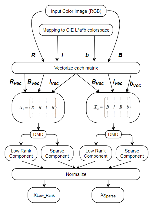
These extracted features capture the underlying dynamics of the image. Therefore, these are then given as input to the Random Kitchen Sink Algorithm (Section II-C) for classification.

IV Results and Discussion

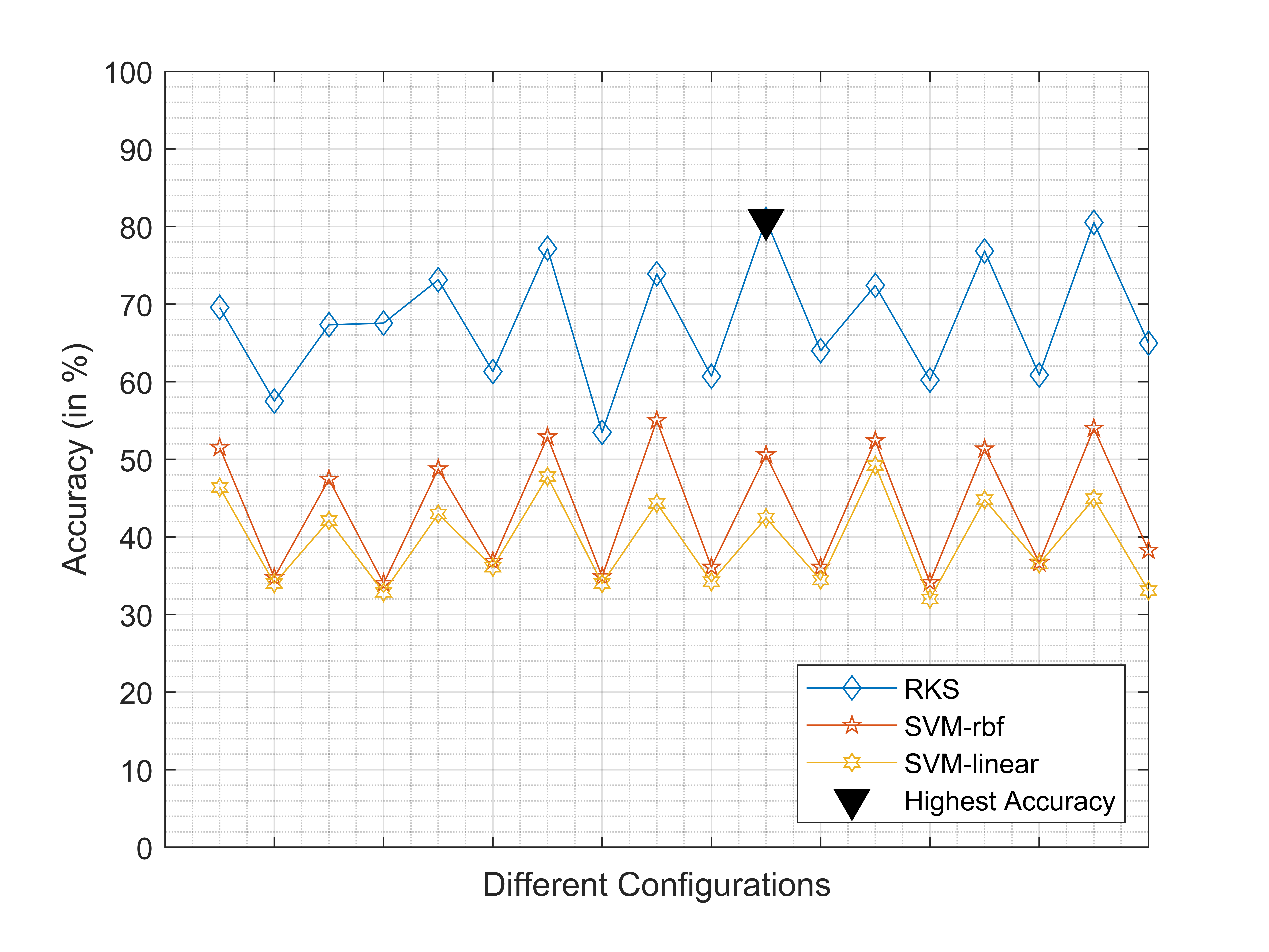
After obtaining the features, they are given as input to the Random Kitchen Sink algorithm and Support Vector Machine (SVM) with various configurations. Tables II, III, IV contain the accuracies of the proposed approach under various configurations when classified by Random Kitchen Sink algorithm, SVM-rbf and SVM-linear respectively. Column 1 represents the percentage of the total dataset used for setting, column 2 represents the count of eigenvalues taken into consideration for reconstruction of the features, column 3 denotes the type of class (Distinctive - Classes that are easily differentiable from one another; Overlapped - Classes that have overlapping features), and column 4 represents the accuracy of the corresponding configuration. All the accuracies corresponding to their configurations are plotted in Figure 4. It is evident from it that the Random Kitchen Sink Algorithm (RKS), constantly comes on top as compared to the other two algorithms.

TABLE II: Accuracy of Random Kitchen Sink Algorithm under different configurations

Test Data (in %)	Number of Eigen Values	Type of Data	Accuracy (in %)
70	3	Distinctive	69.57
70	3	Overlapped	57.50
70	4	Distinctive	67.34
70	4	Overlapped	67.55
70	5	Distinctive	73.14
70	5	Overlapped	61.31
60	3	Distinctive	77.18
60	3	Overlapped	53.47
60	4	Distinctive	73.92
60	4	Overlapped	60.69
60	5	Distinctive	80.87
60	5	Overlapped	64.00
50	3	Distinctive	72.41
50	3	Overlapped	60.20
50	4	Distinctive	76.85
50	4	Overlapped	60.87
50	5	Distinctive	80.52
50	5	Overlapped	64.97

TABLE III: Accuracy of Support Vector Machine (rbf Kernel) under different configurations

Test Data (in %)	Number of Eigen Values	Type of Data	Kernel	Accuracy (in %)
70	3	Distinctive	rbf	51.52
70	3	Overlapped	rbf	34.76
70	4	Distinctive	rbf	47.43
70	4	Overlapped	rbf	34.00
70	5	Distinctive	rbf	48.76
70	5	Overlapped	rbf	36.86
60	3	Distinctive	rbf	52.89
60	3	Overlapped	rbf	34.89
60	4	Distinctive	rbf	55.00
60	4	Overlapped	rbf	36.11
60	5	Distinctive	rbf	50.56
60	5	Overlapped	rbf	36.11
50	3	Distinctive	rbf	52.40
50	3	Overlapped	rbf	34.13
50	4	Distinctive	rbf	51.33
50	4	Overlapped	rbf	36.67
50	5	Distinctive	rbf	54.00
50	5	Overlapped	rbf	38.27

TABLE IV: Accuracy of Support Vector Machine (Linear Kernel) under different configurations

Test Data (in %)	Number of Eigen Values	Type of Data	Kernel	Accuracy (in %)
70	3	Distinctive	linear	46.38
70	3	Overlapped	linear	34.00
70	4	Distinctive	linear	42.10
70	4	Overlapped	linear	32.86
70	5	Distinctive	linear	42.95
70	5	Overlapped	linear	36.10
60	3	Distinctive	linear	47.78
60	3	Overlapped	linear	34.00
60	4	Distinctive	linear	44.33
60	4	Overlapped	linear	34.22
60	5	Distinctive	linear	42.44
60	5	Overlapped	linear	34.44
50	3	Distinctive	linear	49.20
50	3	Overlapped	linear	32.00
50	4	Distinctive	linear	44.80
50	4	Overlapped	linear	36.53
50	5	Distinctive	linear	44.93
50	5	Overlapped	linear	33.07

It is evident from both the Figure 4 and Table II that, the maximum accuracy is attained when the configuration is as follows :

Test Data (in %)	:	60
Number of Eigen Values	:	5
Type of Data	:	Distinctive

Figure 2: 2-Dimensional t-SNE plot of the DMD feature of 50 randomly selected classes with considerations for 5 eigenvalues.

Figure 3: Eigen Value plot of Low rank and sparse matrix

Figure 4: Accuracy plot - RKS Vs SVM-rbf Vs SVM-linear

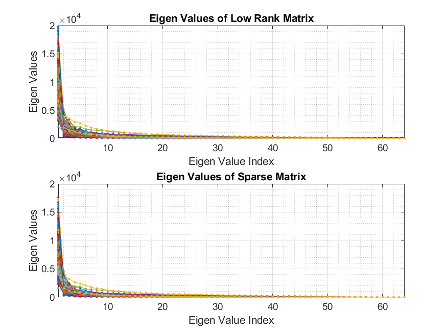
The reason why the accuracy tops when the number of Eigenvalues is “5” can be explained through Figure 3. After the Eigenvalue index of “5”, the Eigenvalues cease to change and doesn’t contribute much to the underlying dynamics of the image. After the features are extracted, it is given as input for RKS in which it is mapped from 640 to 500.

Figure 5: Reconstructed Low-rank ($1^{st}$ row) and Sparse matrix ($2^{nd}$ row) for 5 Eigen Values

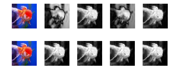
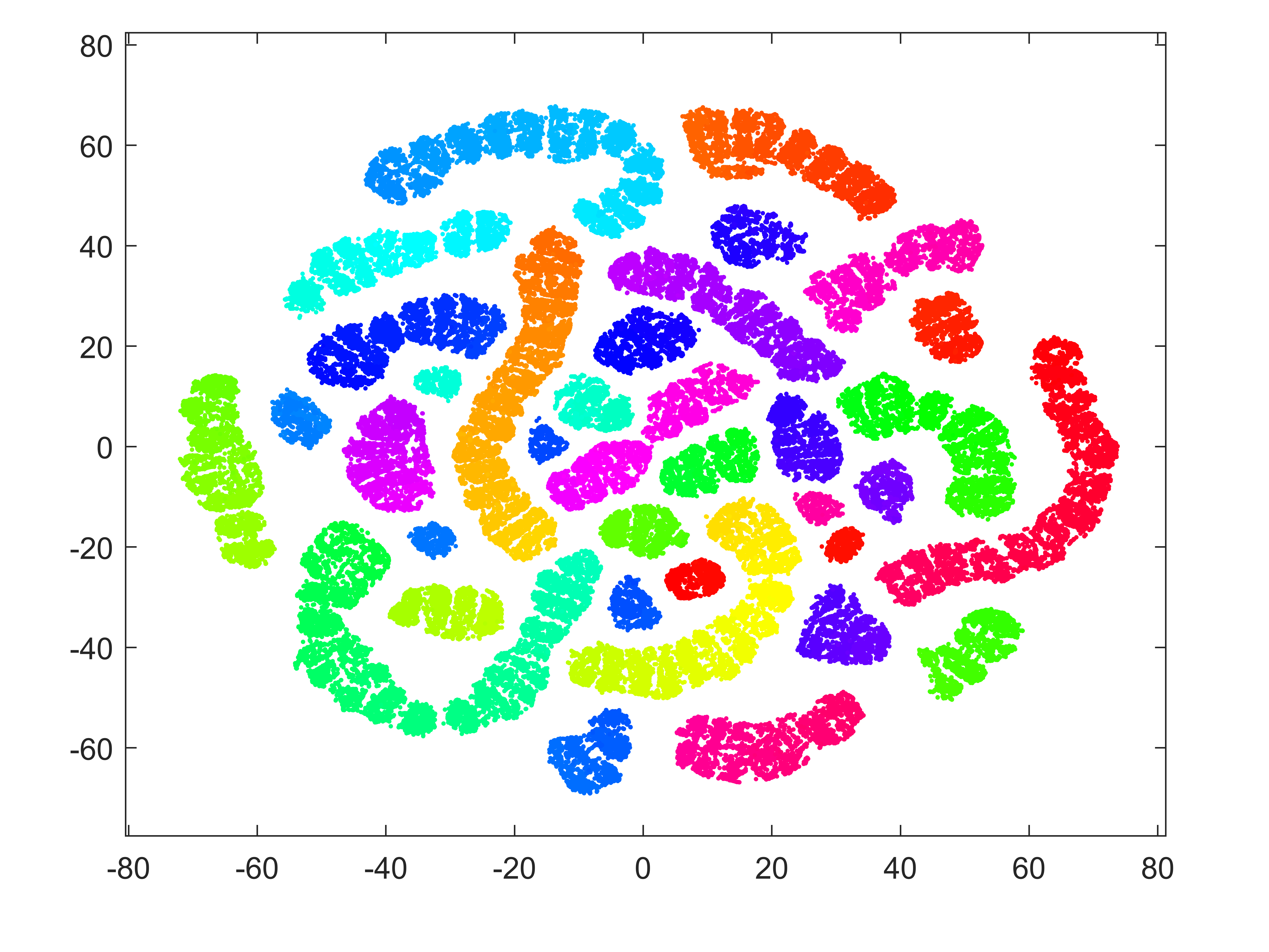
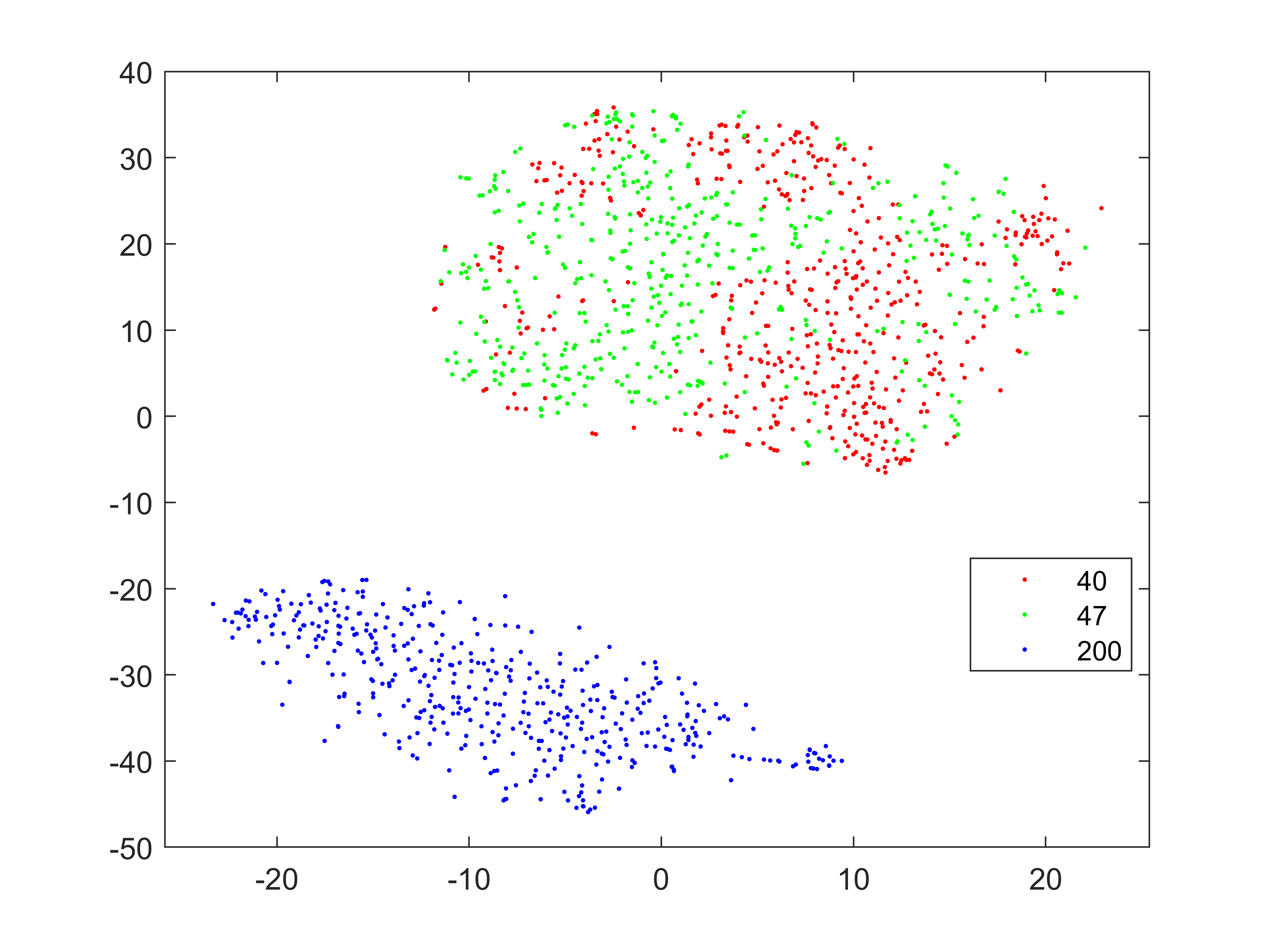
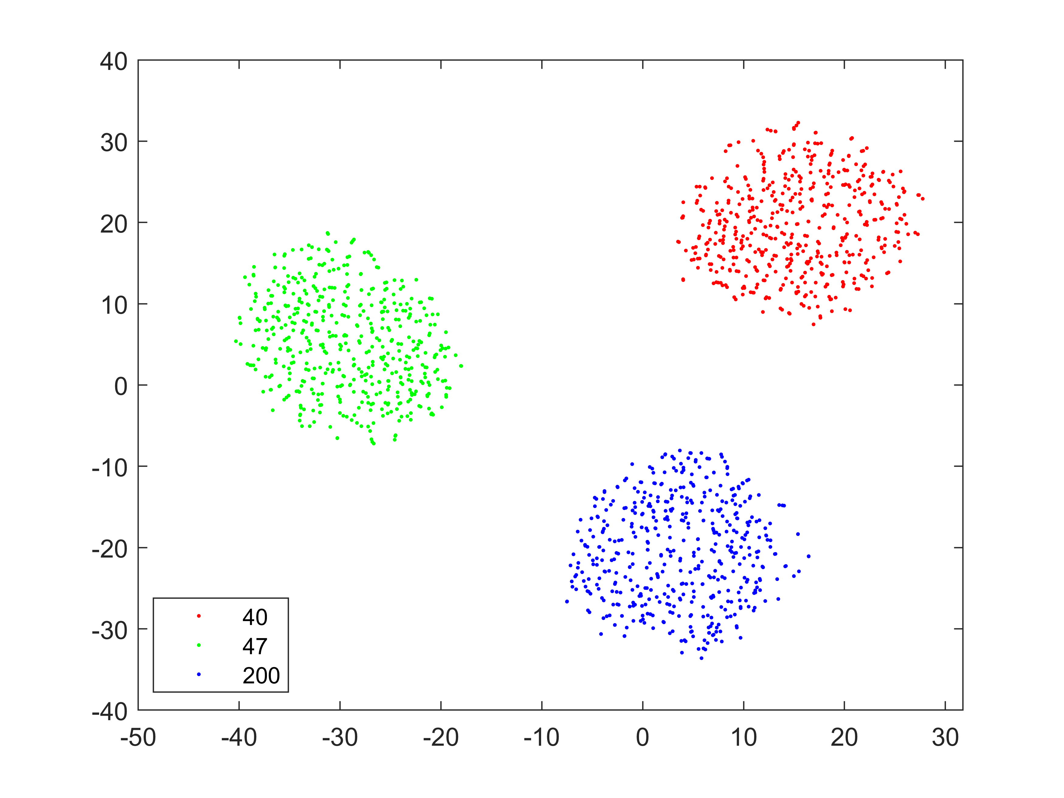
Figure 5 shows the reconstructed image with low-rank and sparse matrix with 5 Eigenvalues which clearly captures the skeleton of the image. This extraction of the skeletal structure is the dynamics captured by applying DMD for feature extraction. t-SNE plot in Figure 2 provides a better picture of how the extracted DMD features of images arrange themselves distinctive groups flawlessly. Figure 6 and Figure 7 are the t-SNE plots of 3 classes before and after applying the proposed technique. It is evident from them that, the proposed approach is promising and effective.

Figure 6: t-SNE plot of 3 classes before applying the proposed approach.

Figure 7: t-SNE plot of 3 classes after applying the proposed approach.

Figure 8: Cases where the proposed approach is ineffective

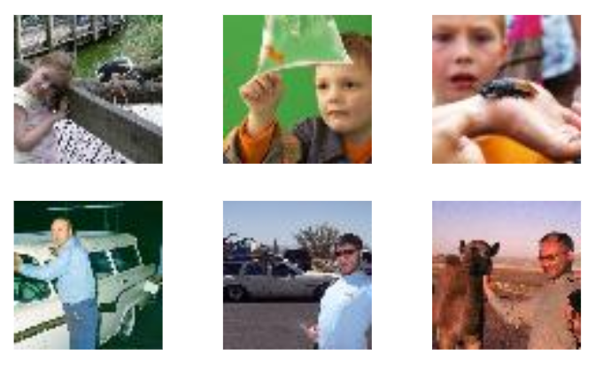
The present approach is a novel one and needs more applications-oriented experimental evaluations. There are certain cases like in Figure 8, which has a complex background and where it is difficult to differentiate the foreground of the object of interest from the background, the proposed approach fails to perform. Apart from cases like in Figure 8, the proposed approach is proven to be effective in learning with limited labelled data.

V Conclusion

As the world’s data generation explodes and due to the reason that manual labelling is highly expensive, it is necessary to develop and explore machine learning architectures that can classify with limited labelled data. The proposed approach in this paper has provided a novel direction in which Dynamic Mode Decomposition based feature can be used in conjunction with a classifier for achieving competing results. As a future scope of this research, the shortcomings of the current proposed architecture can be solved and extended to fast paced applications like Intrusion Detection Systems [51, 52] and Data-driven solvers[53] where the data is limited and the classifier must be re-trained frequently on the go.

References

- [1] Nigam, K., McCallum, A., & Mitchell, T. (2006). Semi-supervised text classification using EM. Semi-Supervised Learning, 33-56.
- [2] Cohen, I., & Cozman, F. G. (2006). Risks of semi-supervised learning: how unlabeled data can degrade performance of generative classifiers.
- [3] Shrivastava, A., Pfister, T., Tuzel, O., Susskind, J., Wang, W., & Webb, R. (2017). Learning from simulated and unsupervised images through adversarial training. In Proceedings of the IEEE Conference on Computer Vision and Pattern Recognition (pp. 2107-2116).
- [4] Goodfellow, I., Pouget-Abadie, J., Mirza, M., Xu, B., Warde-Farley, D., Ozair, S., … & Bengio, Y. (2014). Generative adversarial nets. In Advances in neural information processing systems (pp. 2672-2680).
- [5] Blum, A., & Mitchell, T. (1998, July). Combining labeled and unlabeled data with co-training. In Proceedings of the eleventh annual conference on Computational learning theory (pp. 92-100). ACM.
- [6] Seeger, M. (2000). Input-dependent regularization of conditional density models (No. REP_WORK).
- [7] Nigam, K., & Ghani, R. (2000, November). Analyzing the effectiveness and applicability of co-training. In Cikm (Vol. 5, p. 3).
- [8] Joachims, T. (1999, June). Transductive inference for text classification using support vector machines. In Icml (Vol. 99, pp. 200-209).
- [9] Zhu, X., & Ghahramani, Z. (2002). Learning from labeled and unlabeled data with label propagation (p. 1). Technical Report CMU-CALD-02-107, Carnegie Mellon University.
- [10] Kipf, T. N., & Welling, M. (2016). Semi-supervised classification with graph convolutional networks. arXiv preprint arXiv:1609.02907.
- [11] Saul, L. K., Weinberger, K. Q., Ham, J. H., Sha, F., & Lee, D. D. (2006). Spectral methods for dimensionality reduction. Semisupervised learning, 293-308.
- [12] Erhan, D., Bengio, Y., Courville, A., Manzagol, P. A., Vincent, P., & Bengio, S. (2010). Why does unsupervised pre-training help deep learning?. Journal of Machine Learning Research, 11(Feb), 625-660.
- [13] Pennington, J., Socher, R., & Manning, C. (2014). Glove: Global vectors for word representation. In Proceedings of the 2014 conference on empirical methods in natural language processing (EMNLP) (pp. 1532-1543).
- [14] Mintz, M., Bills, S., Snow, R., & Jurafsky, D. (2009, August). Distant supervision for relation extraction without labeled data. In Proceedings of the Joint Conference of the 47th Annual Meeting of the ACL and the 4th International Joint Conference on Natural Language Processing of the AFNLP: Volume 2-Volume 2 (pp. 1003-1011). Association for Computational Linguistics.
- [15] Takamatsu, S., Sato, I., & Nakagawa, H. (2012, July). Reducing wrong labels in distant supervision for relation extraction. In Proceedings of the 50th Annual Meeting of the Association for Computational Linguistics: Long Papers-Volume 1 (pp. 721-729). Association for Computational Linguistics.
- [16] Urner, R., David, S. B., & Shamir, O. (2012, March). Learning from weak teachers. In Artificial intelligence and statistics (pp. 1252-1260).
- [17] Ratner, A., Bach, S. H., Ehrenberg, H., Fries, J., Wu, S., & Ré, C. (2017). Snorkel: Rapid training data creation with weak supervision. Proceedings of the VLDB Endowment, 11(3), 269-282.
- [18] Dawid, A. P., & Skene, A. M. (1979). Maximum likelihood estimation of observer error‐rates using the EM algorithm. Journal of the Royal Statistical Society: Series C (Applied Statistics), 28(1), 20-28.
- [19] Liu, B., Dai, Y., Li, X., Lee, W. S., & Philip, S. Y. (2003, November). Building Text Classifiers Using Positive and Unlabeled Examples. In ICDM (Vol. 3, pp. 179-188).
- [20] Druck, G., Mann, G., & McCallum, A. (2008, July). Learning from labeled features using generalized expectation criteria. In Proceedings of the 31st annual international ACM SIGIR conference on Research and development in information retrieval (pp. 595-602). ACM.
- [21] Cohn, D. A., Ghahramani, Z., & Jordan, M. I. (1996). Active learning with statistical models. Journal of artificial intelligence research, 4, 129-145.
- [22] Lowell, D., Lipton, Z. C., & Wallace, B. C. (2018). How transferable are the datasets collected by active learners?. arXiv preprint arXiv:1807.04801.
- [23] Siddhant, A., & Lipton, Z. C. (2018). Deep Bayesian active learning for natural language processing: Results of a large-scale empirical study. arXiv preprint arXiv:1808.05697.
- [24] Pan, S. J., & Yang, Q. (2010). A survey on transfer learning. IEEE Transactions on knowledge and data engineering, 22(10), 1345-1359.
- [25] Howard, J., & Ruder, S. (2018). Universal language model fine-tuning for text classification. arXiv preprint arXiv:1801.06146.
- [26] Augenstein, I., & Søgaard, A. (2017). Multi-task learning of keyphrase boundary classification. arXiv preprint arXiv:1704.00514.
- [27] Caruana, R. (1997). Multitask learning. Machine learning, 28(1), 41-75.
- [28] Fei-Fei, L., Fergus, R., & Perona, P. (2006). One-shot learning of object categories. IEEE transactions on pattern analysis and machine intelligence, 28(4), 594-611.
- [29] Socher, R., Ganjoo, M., Manning, C. D., & Ng, A. (2013). Zero-shot learning through cross-modal transfer. In Advances in neural information processing systems (pp. 935-943).
- [30] Xian, Y., Lampert, C. H., Schiele, B., & Akata, Z. (2018). Zero-shot learning-a comprehensive evaluation of the good, the bad and the ugly. IEEE transactions on pattern analysis and machine intelligence.
- [31] Cubuk, E. D., Zoph, B., Mane, D., Vasudevan, V., & Le, Q. V. (2018). Autoaugment: Learning augmentation policies from data. arXiv preprint arXiv:1805.09501.
- [32] Ratner, A. J., Ehrenberg, H., Hussain, Z., Dunnmon, J., & Ré, C. (2017). Learning to compose domain-specific transformations for data augmentation. In Advances in neural information processing systems (pp. 3236-3246).
- [33] Abbeel, P., & Ng, A. Y. (2004, July). Apprenticeship learning via inverse reinforcement learning. In Proceedings of the twenty-first international conference on Machine learning (p. 1). ACM.
- [34] Griffith, S., Subramanian, K., Scholz, J., Isbell, C. L., & Thomaz, A. L. (2013). Policy shaping: Integrating human feedback with reinforcement learning. In Advances in neural information processing systems (pp. 2625-2633).
- [35] Schmid, P. J. (2010). Dynamic mode decomposition of numerical and experimental data. Journal of fluid mechanics, 656, 5-28.
- [36] Rowley, C. W., Mezić, I., Bagheri, S., Schlatter, P., & Henningson, D. S. (2009). Spectral analysis of nonlinear flows. Journal of fluid mechanics, 641, 115-127.
- [37] Rahimi, A., & Recht, B. (2008). Random features for large-scale kernel machines. In Advances in neural information processing systems (pp. 1177-1184).
- [38] Sikha, O. K., Kumar, S. S., & Soman, K. P. (2018). Salient region detection and object segmentation in color images using dynamic mode decomposition. Journal of Computational Science, 25, 351-366.
- [39] Bordes, A., Ertekin, S., Weston, J., & Bottou, L. (2005). Fast kernel classifiers with online and active learning. Journal of Machine Learning Research, 6(Sep), 1579-1619.
- [40] Kumar, S., Mohri, M., & Talwalkar, A. (2012). Sampling methods for the Nyström method. Journal of Machine Learning Research, 13(Apr), 981-1006.
- [41] Fine, S., & Scheinberg, K. (2001). Efficient SVM training using low-rank kernel representations. Journal of Machine Learning Research, 2(Dec), 243-264.
- [42] Rahimi, A., & Recht, B. (2008, September). Uniform approximation of functions with random bases. In 2008 46th Annual Allerton Conference on Communication, Control, and Computing (pp. 555-561). IEEE.
- [43] Pavy, A., & Rigling, B. (2018). SV-Means: A fast SVM-based level set estimator for phase-modulated radar waveform classification. IEEE Journal of Selected Topics in Signal Processing, 12(1), 191-201.
- [44] Schölkopf, B., Smola, A. J., & Bach, F. (2002). Learning with kernels: support vector machines, regularization, optimization, and beyond. MIT press.
- [45] Hofmann, T., Schölkopf, B., & Smola, A. J. (2008). Kernel methods in machine learning. The annals of statistics, 1171-1220.
- [46] Kumar, S. S., Premjith, B., Kumar, M. A., & Soman, K. P. (2015, December). AMRITA_CEN-NLP@ SAIL2015: sentiment analysis in Indian Language using regularized least square approach with randomized feature learning. In International Conference on Mining Intelligence and Knowledge Exploration (pp. 671-683). Springer, Cham.
- [47] Athira, S.; Harikumar, K.; Sowmya, V.; Soman, K.P., Parameter analysis of random kitchen sink algorithm, IJAER, Volume 10, Issue 20, Number 20, p.19351-19355 (2015)
- [48] Thara, S., & Krishna, A. (2018, September). Aspect Sentiment Identification using random Fourier features. In International Journal of Intelligent Systems and Applications (IJISA).
- [49] Mohan, N., Soman, K. P., & Kumar, S. S. (2018). A data-driven strategy for short-term electric load forecasting using dynamic mode decomposition model. Applied energy, 232, 229-244.
- [50] Kumar, S. S., Kumar, M. A., Soman, K. P., & Poornachandran, P. (2020). Dynamic Mode-Based Feature with Random Mapping for Sentiment Analysis. In Intelligent Systems, Technologies and Applications (pp. 1-15). Springer, Singapore.
- [51] Rahul, V. K., Vinayakumar, R., Soman, K. P., & Poornachandran, P. (2018, July). Evaluating Shallow and Deep Neural Networks for Network Intrusion Detection Systems in Cyber Security. In 2018 9th International Conference on Computing, Communication and Networking Technologies (ICCCNT) (pp. 1-6). IEEE.
- [52] Rahul-Vigneswaran, K., Poornachandran, P., & Soman, K.P. (2019). A Compendium on Network and Host based Intrusion Detection Systems. CoRR, abs/1904.03491.
- [53] Rahul-Vigneswaran, K., Mohan, N., & Soman, K.P. (2019). Data-driven Computing in Elasticity via Chebyshev Approximation. CoRR, abs/1904.10434.