The Triplet Resonating Valence Bond State and Superconductivity in Hund’s Metals

Abstract

A central idea in strongly correlated systems is that doping a Mott insulator leads to a superconductor by transforming the resonating valence bonds (RVBs) into spin-singlet Cooper pairs. Here, we argue that a spin-triplet RVB (tRVB) state, driven by spatially, or orbitally anisotropic ferromagnetic interactions can provide the parent state for triplet superconductivity. We apply this idea to the iron-based superconductors, arguing that strong onsite Hund’s interactions develop intra-atomic tRVBs between the t_2g orbitals. On doping, the presence of two iron atoms per unit cell allows these inter-orbital triplets to coherently delocalize onto the Fermi surface, forming a fully gapped triplet superconductor. This mechanism gives rise to a unique staggered structure of onsite pair correlations, detectable as an alternating $\pi$ phase shift in a scanning tunnelling Josephson microscope.

Thirty years ago, Anderson proposed Anderson (1987) the intriguing idea that the resonating valence bonds (RVBs) of a spin liquid could, on doping, provide the fabric for the development of unconventional superconductivity. A key aspect of the RVB theory, is that it departs from weak-coupling approaches to superconductivity, positing that instead of a pairing glue, superconductivity develops from the entangled pairs already present in a spin liquid. RVB theory provides a natural account of the connection between d-wave pairing and antiferromagnetism Lee et al. (2006) in almost-localized systems, a connection that has proven invaluable to the understanding of many families of superconductors, from the cuprate superconductors, to their miniature cousins, the 115 heavy-fermion compounds Thompson and Fisk (2012).

However, to date, there is no counter-part of RVB theory that applies to ferromagnetically correlated materials. There are a wide variety of unconventional superconductors which, to some extent or another, involve strong ferromagnetic (FM) spin correlations. Examples include uranium-based heavy fermion materials Joynt and Taillefer (2002); Pfleiderer (2009) which lie close to a FM quantum critical point, candidate low-dimensional triplet superconductors such as the Bechgaard salts Lang and Mueller (2008), twisted double bilayer graphene Liu et al. (2019); Shen et al. (2019), and various transition metal superconductors Stewart (2011); Hosono et al. (2018), notably the iron-based and ruthenate superconductors, which as Hund’s metals involve strong local FM correlations between orbitals. Various papers have speculated that the Hund’s interactions might provide the origin of the pairing in these systems Puetter and Kee (2012); Hoshino and Werner (2015); Vafek and Chubukov (2017); Cheung and Agterberg (2019); Anderson (1985); Norman (1994).

Is there a ferromagnetic analog to the RVB pairing mechanism? Here we build on an observation Shen et al. (2020) that magnetic anisotropy in a ferromagnet plays an analogous role to frustration in an antiferromagnet (AFM), generating a fluid of triplet resonating valence bonds (tRVBs). We propose that like their singlet cousins, tRVB states can, on doping, lead to the development of triplet pairing. One of the exciting features of this idea, is that tRVBs can form within the interior of Hund’s coupled atoms, which under the right symmetry conditions Anderson (1985); Hotta and Ueda (2004) can coherently tunnel into the bulk to develop triplet superconductivity Yin et al. (2011); Georges et al. (2013).

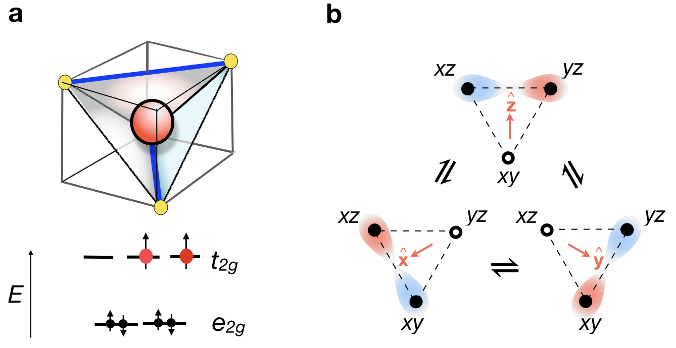
Figure 1: a) Isolated tetrahedron in iron-based superconductors, showing the two electrons forming a $S=1$ triplet in the t_2g orbitals. c) Triplet resonating valence bond (tRVB) as the ground state of a Hund’s metal atom. The blue and red colors reflect the odd parity of the triplet pairs, while the red arrows denote the quantization axis (d-vector) of the $m=0$ triplet pair.

Consider an easy-plane FM interaction $H_{ij}=-J\vec{S}_{i}\cdot\vec{S}_{j}+\Delta JS^{z}_{i}S^{z}_{j}$, ($J>0$) between two spin-1/2 moments $\vec{S}_{i}$ and $\vec{S}_{j}$. In the Heisenberg limit ($\Delta J=0$) and in the presence of a small symmetry breaking Weiss field, the ground-state is a product state which lacks entanglement. Suppose the magnetization points in the $x$ direction, the product ground-state can then be written in terms of triplets,

$$\frac{\left|\uparrow_{i}\right\rangle+\left|\downarrow_{i}\right\rangle}{\sqrt{2}}\frac{\left|\uparrow_{j}\right\rangle+\left|\downarrow_{j}\right\rangle}{\sqrt{2}}=\frac{\left|\uparrow_{i}\uparrow_{j}\right\rangle+\left|\downarrow_{i}\downarrow_{j}\right\rangle}{2}+\frac{\left|\uparrow_{i}\downarrow_{j}\right\rangle+\left|\downarrow_{i}\uparrow_{j}\right\rangle}{2}.$$ (1)

An easy-plane anisotropy ($\Delta J>0$) projects out the equal-spin pairs on the right-hand-side, stabilizing an entangled spin-1 ground state with $m_{z}=0$. In the corresponding easy-plane ferromagnet, with Hamiltonian $H=\sum_{(i,j)}H_{ij}$, the intersite couplings preserve the $m_{z}=0$ structure of the valence bonds, and the resulting ground-state is a quantum superposition of triplet pairs which retains its ferromagnetic correlations, and may even exhibit long-range order.Sup

Our interest in a tRVB ground-state lies in its potential as a pre-entangled parent state of a triplet superconductor. In classic RVB theory, an antiferromagnetic superexchange interaction, is decoupled in terms of singlet pairs Kotliar and Liu (1988):

$$J\vec{S}_{i}\cdot\vec{S}_{j}\equiv-\frac{J}{2}\bigl{(}\psi^{\dagger}_{i\uparrow}\psi^{\dagger}_{j\downarrow}-\psi^{\dagger}_{i\downarrow}\psi^{\dagger}_{j\uparrow}\bigr{)}\bigl{(}\psi_{j\downarrow}\psi_{i\uparrow}-\psi_{j\uparrow}\psi_{i\downarrow}\bigr{)},$$ (2)

where we have used a fermionic representation of the spins, $\vec{S}_{j}=\psi_{j}^{\dagger}\left(\frac{\vec{\sigma}}{2}\right)\psi_{j}$. The corresponding relation for triplet valence bonds is obtained by rotating the spin co-ordinate system at site $j$ through 180^∘ about the z-axis, which gives

$$- J_{A}(S^{x}_{i}S^{x}_{j}+S^{y}_{i}S^{y}_{j}-S^{z}_{i}S^{z}_{i})$$ (4)

$$\equiv-\frac{J_{A}}{2}\bigl{(}\psi^{\dagger}_{i\uparrow}\psi^{\dagger}_{j\downarrow}+\psi^{\dagger}_{i\downarrow}\psi^{\dagger}_{j\uparrow}\bigr{)}\bigl{(}\psi_{j\downarrow}\psi_{i\uparrow}+\psi_{j\uparrow}\psi_{i\downarrow}\bigr{)},$$

demonstrating how xy anisotropy stabilizes a triplet pair.

The most direct application of the tRVB idea considers an easy-plane Heisenberg ferromagnet: by analogy with the singlet RVB pairing mechanism, doping with holes drives the formation of a triplet superconductor. On a square lattice, this scenario leads to a p_x+ ip_y triplet superconductor, to be presented elsewhere. A more dramatic possibility, in which $i$ and $j$ represent orbitals of a single atom, permits us to apply the tRVB idea to Hund’s coupled metals. Here an application of particular current interest, is as a theory for iron-based superconductors (FeSC).

The family of FeSC are characterized by high transition temperatures with a fully gapped Fermi surface. The presence of antiferromagnetic correlations and a marked Knight shift has led to the long-held assumption that these materials are spin singlet superconductors Mazin et al. (2008); Stewart (2011). On the other hand, the recent observation Lee et al. (2018) of a robust ratio $2\Delta/T_{c}\sim 7.2$ between the gap $\Delta$ and the transition temperature $T_{c}$ across a broad range of FeSC motivates the search for a common pairing mechanism, one that is robust against the wide spectrum of Fermi surface morphologies, and hence most likely rooted in the local electronic structure of the iron atoms. Here, we propose that these systems are tRVB superconductors, with a fully gapped Fermi surface, an anisotropic Knight shift and an alternating pair wave-function.

The symmetry properties of a Hund’s coupled triplet superconductor were first considered by Anderson Anderson (1985), who observed that in systems with a center of inversion, the odd-parity wavefunction of a triplet condensate prevents onsite triplet pairing unless the lattice has an even number of atoms per unit cell, related to each other via inversion. In this situation, the odd-parity nature of the condensate means that the onsite pair wavefunction reverses sign when reflected through the center of inversion

$$\langle\psi_{a\sigma}(\mathbf{x})\psi_{b\sigma^{\prime}}(\mathbf{x})\rangle=-\langle\psi_{a\sigma}(-\mathbf{x})\psi_{b\sigma^{\prime}}(-\mathbf{x})\rangle,$$ (5)

where $a$ and $\sigma$ are the orbital and spin indices, respectively. The key structural feature of FeSC is an iron atom enclosed in a tetrahedral cage of pnictogen or chalcogen atoms. The tetrahedra are packed in a checker-board arrangement, with a unit cell containing two iron atoms, separated by a common center of inversion, satisfying this requirement. We now show how tRVB predicts a condensate with the above properties.

In the parent compound of the FeSC, each tetrahedron contains two electrons within the three $xz,yz$ or $xy$ orbitals of the $t_{2g}$ level, Hund’s coupled into a $S=1$, $L=1$ manifold. Consider the “atomic” limit of an isolated iron tetrahedron. Each pair of $t_{2g}$ orbitals shares a common direction, for instance, the $xz$ and $yz$ orbitals share a common $z$ axis, which in the presence of spin-orbit coupling causes Sup the Hund’s interactions to develop an orbitally selective easy-plane anisotropy (Eq. 4),

$$H_{I} = -2\Big{[}(J_{H}+J_{\rm A})\vec{S}_{xz}\cdot\vec{S}_{yz}-2J_{\rm A}S^{z}_{xz}S^{z}_{yz})$$ (6)

$$\hskip 71.13188pt+(\hbox{cyclic permutations)}\Big{]}.$$

Each of the three interaction terms stabilizes a triplet pair with zero spin component along a quantization axis (“d-vector”) normal to its easy-plane (See Fig. 1c), thus the xz and xy orbitals have d-vector $\hat{d}=\hat{x}$.

With the convention $a\in\{xz,yz,xy\}=\{1,2,3\}$, the projected angular momentum operator within the $t_{2g}$ subspace is $(L_{a})_{bc}\equiv{-}i\epsilon_{abc}$. Defining the triplet pair creation operators $\Psi^{\dagger}_{ab}\equiv\psi^{\dagger}({L}_{a}\sigma_{b})\bar{\psi}^{\dagger}$, $a,b={1,2,3}$, where $\bar{\psi}^{\dagger}\equiv i\sigma_{2}(\psi^{\dagger})^{T}$, Eq. (6) can be written using summation convention as $H_{\rm I}=-g_{ab}\Psi^{\dagger}_{ab}\Psi_{ab},$ with $g_{ab}=\frac{1}{4}(J_{H}+J_{\rm A}\delta_{ab})$. In this way, we see that an anisotropy $J_{\rm A}>0$ splits off a ground-state manifold of triplet pairs in which the orbital angular momenta and the spin quantization axis are aligned, $\Psi^{\dagger}_{aa}\left|0\right\rangle=\psi^{\dagger}(\sigma_{a}L_{a})\bar{\psi}^{\dagger}\left|0\right\rangle$.

The spin-orbit coupling $H_{SL}=-\lambda\vec{L}\cdot\vec{S}$ causes the triplet valence bonds to resonate between orbitals, giving rise to a tRVB ground state $\left|\text{tRVB}\right\rangle=\sum_{ab}\Lambda^{ab}\Psi^{\dagger}_{ab}|0\rangle$ (see Fig. 1b). Note that within the t_2g multiplet, the projected spin orbit interaction has a reversed coupling constant, with $\lambda>0$, favoring $L+S=2$ configurations. The structure of the resulting energy levels is modelled by a crystal field Hamiltonian given by $H=-\lambda(\vec{L}\cdot\vec{S})-\alpha(J_{x}^{4}+J_{y}^{4}+J_{z}^{4})+\eta J_{z}^{2}$, where $J=S+L$ is the total angular momentum, $\alpha\sim J_{A}$, while $\eta$ quantifies the tetragonal anisotropy of the environment. The simplest tRVB ground-state, where ${\Lambda}_{ab}=\delta_{ab}$ is a unit matrix, develops for the wrong sign of the spin-orbit coupling $\lambda<0$. Two other tRVB states with $\Lambda_{ab}={\rm diag}(1,-1,0)$ and $\Lambda_{ab}={\rm diag}(1,1,-2)$ are stabilized for $\lambda>0$, Sup , where the latter becomes the unique ground-state in the presence of a tetragonal anisotropy $\eta>0$, see Fig. (1b).

When the tetrahedra are brought together to form a conductor, charge fluctuations allow the escape of atomic triplet pairs into the conduction sea. We shall assume that the interactions present in the isolated tetrahedra are preserved in the metallic state that now develops. Imagine a lattice where the $xy$ orbitals are weakly hybridized with the $xz$/$yz$ orbitals at neighboring sites (we denote this amplitude as $t_{7}$). An onsite valence bond between an $xz$ and $xy$ orbital can tunnel to the neighboring site in a two step process: an $xz$ electron first hops to a neighboring $xy$ orbital, forming an intersite, intraorbital triplet pair, after which the $xy$ electron follows suit and hops onto the neighboring site to reassemble the intra-atomic triplet bond. In fact, the electrons can tunnel in either order and the resulting tumbling motion of the tRVB causes its amplitude to alternate at neighboring sites. If this process becomes coherent, it leads to a staggered anomalous triplet pairing amplitude (see eq 5) $\Delta({\bf{x}})=-\Delta(-{\bf{x}})$ as envisioned in Anderson (1985) (see Fig. 2a). For this motion to be sustained coherently, there must be two atoms per unit cell. To understand how this works in the FeSC, we note there is an additional non-symmorphic symmetry Lee and Wen (2008), under which the lattice is invariant under a glide and mirror reflection through the plane. The opposite parities of the $xy$ and $xz$/$yz$ orbitals under glide reflection, means that the inter-orbital tunneling amplitude $t_{7}$ alternates (see Fig. 2b). When the $xz$/$xy$ and $yz$/$xy$ pairs tunnel left, or right into the conduction sea, they do so with opposite amplitudes, causing the intersite, intraorbital triplet pairs to coherently condense in the same direction. This permits the phase-alternating tRVB pairs to coherently escape onto the Fermi surface (see Fig. 2c), activating a logarithmic Cooper divergence in the pair susceptibility. The non-symmorphic symmetry of the FeSC allows us to absorb the staggered hopping into a staggered gauge transformation of the $xz$/$yz$ orbitals Daghofer et al. (2010), $\psi_{xz/yz}({\bf j})\rightarrow(-1)^{j_{x}+j_{y}}\psi_{xz/yz}({\bf j})$. This transformation unfolds the Brillouin zone and allows to treat each iron atom on an equal footing.

Following Anderson (1987) we introduce the simplest tRVB wave function as the Gutzwiller projection of a BCS-like wave function

$$|\hbox{tRVB}\rangle=\hat{P}_{G}\prod_{\mathbf{k}}\text{exp}\left(\psi^{\dagger}_{\mathbf{k}}[\vec{\mathcal{L}}(\mathbf{k})\cdot\vec{\sigma}]\bar{\psi}^{\dagger}_{-\mathbf{k}}\right)\left|0\right\rangle.$$ (7)

Here $P_{G}$ is the Gutzwiller projector to $n<2$ electron per site. The functions $\vec{\cal L}=\sum_{g}\vec{\Lambda}_{g}({\bf{k}})\lambda_{g}$ with $g=1...8$ can be expanded in the eight-fold space of Gell-Mann matrices which span the t_2g multiplet. The triplet character of the condensate means that ${\cal L}(-{\bf{k}})=-{\cal L}^{T}({\bf{k}})$, so the three anti-symmetric $\lambda_{g}\in\{L_{a}\}_{a=1}^{3}$ matrices combine with even parity functions $\Lambda_{s}({\bf{k}})=\Lambda_{s}(-{{\bf{k}}})$ to describe the onsite, orbitally antisymmetric pairing, while the five symmetric $\lambda_{g}$, combine with odd-parity p-wave functions $\Lambda_{a}({\bf{k}})=-\Lambda_{a}(-{\bf{k}})$, to describe the tRVBs that have escaped to the Fermi surface.

To calculate the properties of the tRVB wavefunction, we adopt a Gutzwiller mean field approach, assuming that the action of the microscopic Hamiltonian beneath the projection operator $P_{G}$ can be modelled by an appropriate renormalization of hopping matrix elements in a mean-field Hamiltonian. A microscopic rationale for these renormalizations can be obtained from a slave boson treatment of the unprojected Hamiltonian, along the lines of RVB theory Kotliar and Liu (1988); Komijani et al. . Here we concentrate on the weak-coupling Cooper instability that arises from the renormalized Hamiltonian. Motivated by our discussion of the isolated tetrahedron, we now rewrite the Hund’s interaction, Eq. (6) in the form of a BCS theory

$$H_{I}=\sum_{\mathbf{x},ab}\Big{[}\frac{1}{g_{ab}}\bar{\Delta}_{ab}{{\Delta}_{ab}}+(\Psi^{\dagger}_{ab}{\Delta}_{ab}+h.c.)\Big{]}.$$ (8)

For $t_{2g}$ materials, the states at the Fermi surface are composed of three component Bloch wave functions $\vec{u}_{n,\mathbf{k}}$ which are eigenstates of the kinetic term $H_{\rm kin}(\mathbf{k})\vec{u}_{n,\mathbf{k}}=\epsilon_{n}(\mathbf{k})\vec{u}_{n,\mathbf{k}}$. On the Fermi surface, the band-diagonal matrix element of the gap function is given by $\vec{d}_{n{\bf{k}}}\cdot\vec{\sigma}$, where the d-vector is $d^{a}_{n{\bf{k}}}\equiv\Delta_{ab}(\vec{u}_{n,-\mathbf{k}}^{T}L_{b}\vec{u}_{n,\mathbf{k}})=-i\Delta_{ab}(\vec{u}_{n,-\mathbf{k}}\times\vec{u}_{n,\mathbf{k}})_{b}$. The d-vector vanishes if the Bloch wave function $\vec{u}_{n-{\bf{k}}}=\vec{u}_{n{\bf{k}}}$ is symmetric, since $\vec{u}_{n,\mathbf{k}}\times\vec{u}_{n,\mathbf{k}}=0$. Fortunately, the non-symmorphic character of the lattice mixes the $xy$ and $xz$/$yz$ orbitals, so that $\vec{u}_{n{\bf{k}}}\neq\vec{u}_{n-{\bf{k}}}$, which allows the d-vector to be finite.

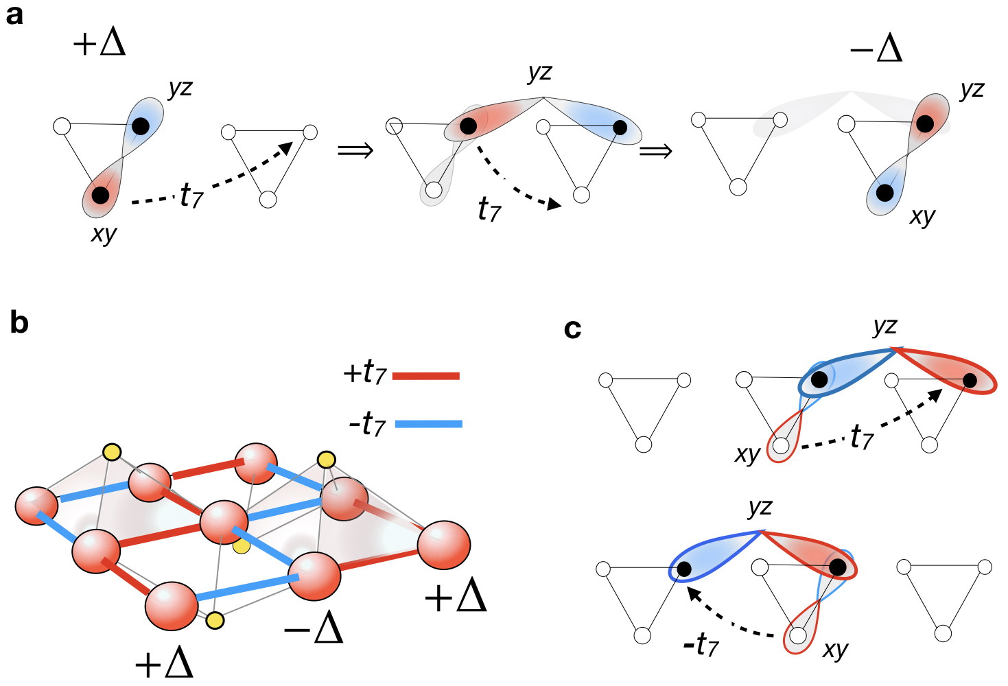
Figure 2: Schematic showing a) how tunneling of a triplet valence bond between two iron atoms leads to “tumbling” motion that reverses the onsite triplet pair amplitude $\Delta$ on neighboring iron atoms, b) the alternation in the sign of inter-orbital hopping $t_{7}$ and onsite triplet pairing, c) how the asymmetric left and right tunneling permits triplet pairs to align in the same direction between sites, allowing them to coherently condense into a p-wave state on the Fermi surface.

The simplest mean-field theory, corresponding to $\Delta_{ab}=\Delta{\rm diag}(1,1,-2)$, models the iron-based superconductors as a two dimensional conductor with Hamiltonian

$$H_{\rm BCS} = {\frac{|\Delta|^{2}}{g}+\frac{1}{V}\sum_{{\bf{k}}}\tilde{\psi}_{{\bf{k}}}^{\dagger}\Big{[}H_{\rm kin}(\mathbf{k})\tau_{3}}$$ (9)

$$\hskip 42.67912pt{+\Delta(\sigma_{1}L_{1}+\sigma_{2}L_{2}-2\sigma_{3}L_{3})\tau_{1}\Big{]}\tilde{\psi}_{{\bf{k}}}}.\qquad$$

Here $\tilde{\psi}_{{\bf{k}}}$ is a Nambu spinor in the space of orbital, spin and charge (isospin) space. The pairing term $(\sigma_{1}L_{1}+\sigma_{2}L_{2})\tau_{1}$ term retains the essential tRVB pairing components that mix the $xy$ and $xz$/$yz$ orbitals at the Fermi surface and is sufficient to gap out the Fermi surface. In our two dimensional model the component $\sigma_{3}L_{3}\tau_{1}$ has no weak-coupling support on the Fermi surface but induces inter-band pairing between $xz$ and $yz$ orbitals Vafek and Chubukov (2017). The term

$$H_{\rm kin}({{\bf k}})=\epsilon_{{\bf{k}}}+\vec{\epsilon}_{{\bf{k}}}\cdot\vec{\gamma}=\left(\begin{array}[]{cc|c}a_{{\bf{k}}}&g_{{\bf{k}}}&ip_{k_{x}}\cr g_{{\bf{k}}}&b_{{\bf{k}}}&ip_{k_{y}}\cr\hline\cr-ip_{k_{y}}&-ip_{k_{x}}&e_{{\bf{k}}}\end{array}\right),$$ (10)

describes the band-dispersion Daghofer et al. (2010), where $a_{{\bf{k}}}=2t_{1}c_{x}+2t_{2}c_{y}+4t_{3}c_{x}c_{y}-\mu$, $b_{{\bf{k}}}=2t_{2}c_{x}+2t_{1}c_{y}+4t_{3}c_{x}c_{y}-\mu$, $g_{{\bf{k}}}=4t_{4}s_{x}s_{y}$, $p_{k_{x}}=2t_{7}s_{x}+4t_{8}s_{x}c_{y}$, $p_{k_{y}}=2t_{7}s_{y}+4t_{8}s_{y}c_{x}$ and $e_{{\bf{k}}}=2t_{5}(c_{x}+c_{y})+4t_{6}c_{x}c_{y}-\mu+\delta_{xy}$, and we have employed the short-hand notation $c_{l}\equiv\cos k_{l}$ and $s_{l}=\sin k_{l}$ (l=x,y).

Although the pairing in this mean-field theory is uniform, if we undo the gauge transformation of the $xz$/$yz$ states, the onsite pairing between the $xy$ and $xz$/$xy$ states acquires the staggered behavior predicted by Anderson. Remarkably, even though this order parameter is staggered, it induces a gap on the Fermi surface, with a pair susceptibility that is logarithmically divergent at low temperatures.

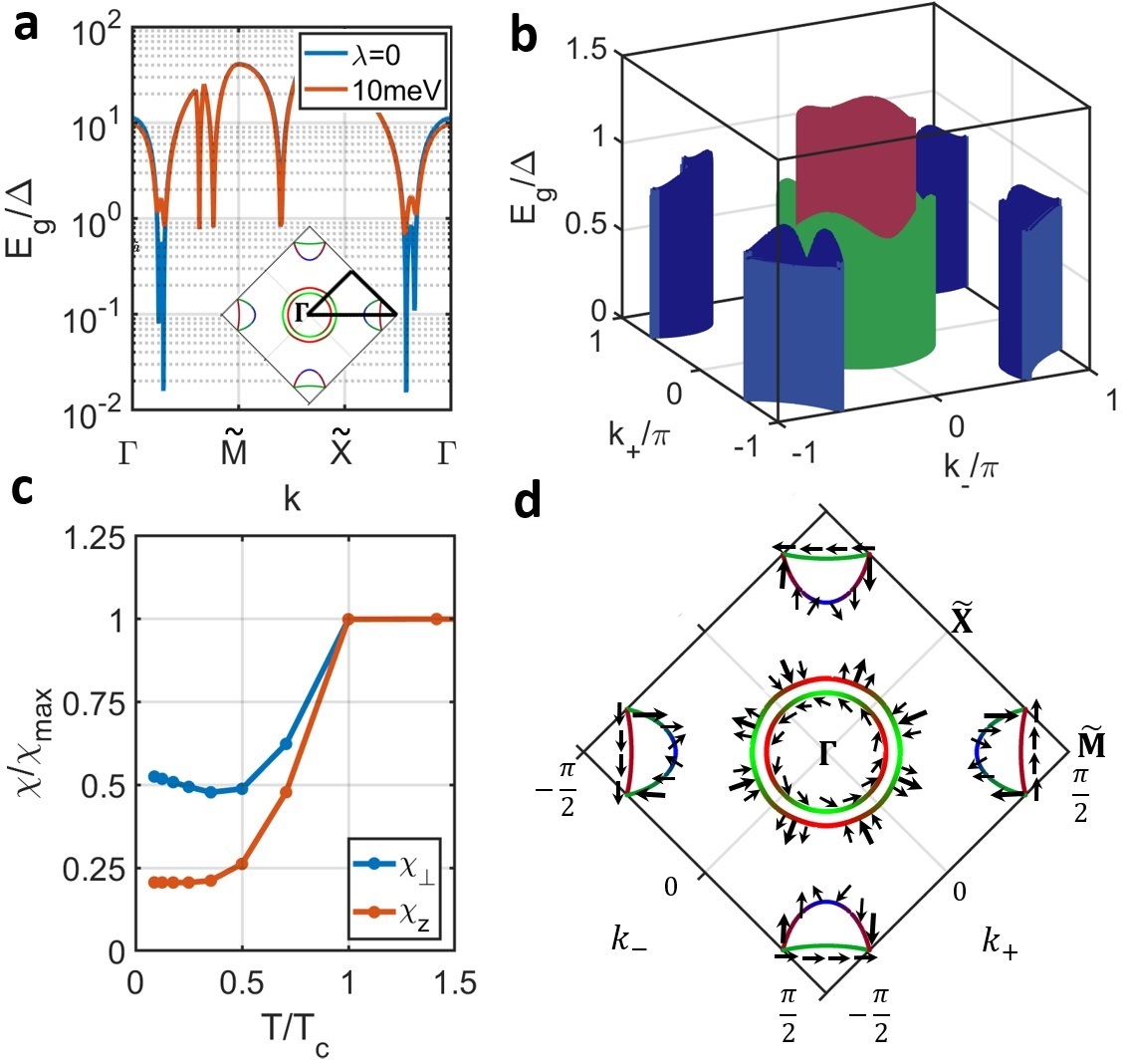
Figure 3: a) The size of the gap along a cut passing high-symmetry points in the Fermi surface (FS), for $\Delta=6.2$meV for $\lambda_{SO}=0$ and $\lambda=10$meV. The inset shows the folded Brillouin zone with with $k_{\pm}=(k_{x}\pm k_{y})/2$ and $\tilde{X}=(\pi,0)$ and $\tilde{M}=(\pi/2,\pi/2)$. b) The size of the gap on the FS for $\Delta=6.2$meV and $\lambda_{SO}=10$meV. c) The normalized spin-susceptibility at the transition for $\Delta=6.2$meV and $\lambda_{SO}=$ 10meV Borisenko et al. (2016). d) The winding of the $\vec{d}({\bf k})$ vector along the FS for $\lambda_{SO}=0$ illustrates p-wave ($E_{u}$) pairing. Note that $\vec{d}$ vector is entirely in the plane in this case.

Figs. 3 a,b display the spectrum calculated from the mean-field theory Eq. (9) using tight binding parameters of Ref. Daghofer et al. (2010) and $t_{8}=-t_{7}/3$. The ground-state develops an anisotropic, yet full gap on the Fermi surface which becomes increasingly isotropic with the introduction of spin-orbit coupling. Historically, the observation of a full gap Sprau et al. (2017); Kushnirenko et al. (2018); Hashimoto et al. (2018) and the presence of a finite Knight shift in all field directions led to an early rejection of the idea of triplet pairing in FeSC. However, the calculated Knight-shift, obtained by summing both Fermi surface and inter-band components of the total spin and orbital susceptibility (Fig. 3c), shows a marked loss of spin susceptibility for all field directions, in accord with experiment. We note that in a two dimensional model, the staggered hopping $t_{7}$ that delocalizes the pairs is only present in the basal plane. When motion in the c-axis is included, the additional staggered hopping along the c-axis will now hybridize the $xz/yz$ orbitals, introducing an additional $p_{z}$ component to the condensate, further reducing the predicted anisotropy.

Various other aspects of the tRVB theory of pairing in FeSC deserve discussion. First, since the Hund’s triplet pairing occurs locally on the iron atom, (unlike, $s_{\pm}$ pairing), tRVB accounts for intra-atomic Coulomb repulsion without relying on a cancellation between electron and hole pockets  König and Coleman (2019). Second, because this pairing is local, it is expected to be moderately robust against the pair breaking effects of impurity scattering. Microscopically, disorder generates non-zero vertex corrections to the local pair which partially cancel the disorder induced self energy Sup , thereby reducing the pair-breaking effets of disorder. Third, there are multiple sign changes of the triplet d-vectors on and in between the various Fermi surfaces (Fig. 3d). The finite winding number of the d-vector around each pocket may lead to interesting topological behavior. At the same time the relative sign between d-vectors on electron and hole pockets gives rise to quasiparticle coherence factors which closely resemble those of an $s_{+-}$ superconductor with important consequences for quasiparticle interference (QPI) Hanaguri et al. (2010); Chi et al. (2014) and neutron spin resonance measurements . Specifically, the dominant Fermi surface contribution to the antisymmetrized tunneling density of states at wave vector ${\bf q}$ is proportional to the Fermi surface (FS) average $\langle 1-\hat{d}_{n}({\bf k}+{\bf q})\cdot\hat{d}_{m}({\bf k})\rangle_{{\bf k}\in\rm FS}$, with $\hat{d}=\vec{d}/|\vec{d}|$. Features in this observable were previously interpreted as evidence for $s_{\pm}$ pairing, but our estimate suggests that tRVB is also consistent. A more detailed expression and a discussion of a similar feature on the subgap spin-resonance Christianson et al. (2008) are relegated to Ref. Sup .

A key feature of tRVB is the prediction that Hund’s pairing will give rise to a staggered superconductor. The manifestation of this state in FeSC and other candidate materials, would be most naturally detected as a spatial modulation in the relative phase of the Josephson current measured in a scanning tunneling Josephson microscope, using two superconducting STM tips of the same tRVB material. The alternating superconducting phase is predicted to lead to a staggered $\pi$-junction behavior as the tip is swept across the material Sup .

Finally, we mention the possible relevance of tRVB to other superconductors of current interest. The recent discovery of the heavy-fermion UTe₂, which has an even number of uranium atoms per unit cell, with likely triplet superconductivity Ran et al. (2019) is one promising example. Another intriguing candidate material is magic angle double bilayer graphene, where the valley degrees of freedom play the role of orbitals, giving rise to Hund’s coupled interorbital triplet pairing Scheurer et al. (2019) on a moiré superlattice.

Acknowledgments: The authors gratefully acknowledge discussions with Po-Yao Chang. Piers Coleman and Elio König are supported by DOE Basic Energy Sciences grant DE-FG02-99ER45790. Yashar Komijani was supported by a Rutgers Center for Materials Theory postdoctoral fellowship. All authors contributed equally to this work.

Supplementary Information

These supplemental materials include a section on the preservation of triplet (tRVB) states under time evolution (Sec. I), a discussion of the role of symmetries and impurity scattering (Sec. II), and a study of observables for the iron-based superconductors, including the local density of states, Knight shift and a proposal for the detection of the staggered superconducting phase using scanning tunneling Josephson microscopy (Sec. III).

I Preservation of $t$RVB states under time evolution

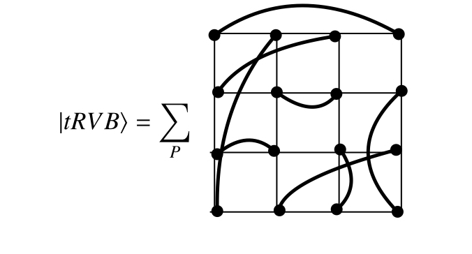
Figure 4: Bond configurations in a tRVB wavefunction.

The concept of the tRVB state relies on the observation that the ground-state xy-anisotropic Ferromagnet, with Hamiltonian $H=\sum_{(i,j)}H_{ij}$, where

$$H_{ij}=-J(\vec{S}_{i}\cdot\vec{S}_{j})+\Delta JS^{z}_{i}S^{z}_{j}$$ (11)

is a resonating valence bond state of triplet pairs (see Fig. 4), given by a weighted sum over bond configurations

$$|{\rm tRVB}\rangle = \sum_{P}A_{P}|P\rangle,$$ (12)

$$|P\rangle = \prod_{(i,j)\in P}|(i,j)\rangle.$$ (13)

Here $A_{P}$ is the amplitude for a given configuration $|P\rangle$ of triplet valence bonds (tVBs) and $|(i,j)\rangle\equiv(|\uparrow\rangle_{i}|\downarrow\rangle_{j}+|\downarrow\rangle_{i}|\uparrow\rangle_{j})/\sqrt{2}$ is an $m=0$ triplet valence bond formed between sites $i$ and $j$. In contrast to its singlet cousin, which has been extensively studied, the properties of tRVB ground-states are largely unexplored. One of the important points that was learned from the study of RVB ground-states, is that even nearest neighbor, “dimer” coverings can exhibit off-diagonal long range antiferromagnetic order (see eg. Albuquerque et al. (2012)). Similar behavior is expected for the dimer tRVB state.

The consistency of tRVB theory requires that the action of the Hamiltonian on any configuration of the triplet valence bonds (tVBs) is closed within the space of tVBs, i.e that the action of the Hamiltonian on a given bond, $H_{ij}$ lies exclusively within the space of states $\left\{|P\rangle\right\}$, so that $H_{ij}|P\rangle=\sum_{P^{\prime}}|P^{\prime}\rangle h^{P^{\prime}P}(ij)$. We can rewrite the isotropic part of the Hamiltonian in terms of the spin exchange operator $P_{ij}$,

$$H_{ij}=-({J}/{2})P_{ij}+\Delta JS^{z}_{i}S^{z}_{j}+J/4.$$ (14)

The action of $P_{ij}$ permutes the ends of the valence bonds, so it is closed within the Hilbert space of tVBs, however the action of the additional Ising component $H^{I}_{ij}=\Delta JS^{z}_{i}S^{z}_{j}$ needs to be considered with care.

There are two configurations of the tVBs to consider (Fig. 5). If there is a triplet valence bond between $i$ and $j$, then it is unaffected by the Ising term $S^{z}_{i}S^{z}_{j}|(i,j)\rangle=-\frac{1}{4}|(i,j)\rangle$(Fig. 5a). If however, there is no bond between sites $i$ and $j$, then we must have two separate tVBs, one linked to site $i$, the other to site $j$. In this situation, the Ising term has the effect of converting two triplet bonds ending at $i,j$ into two singlet bonds which at first sight, suggests that the space of tVBs is not closed under the action of $H_{ij}$. However, we now demonstrate that the space is closed. To this end we carefully take into account the overcompleteness of the basis of valence bonds states. (Fig. 5b).

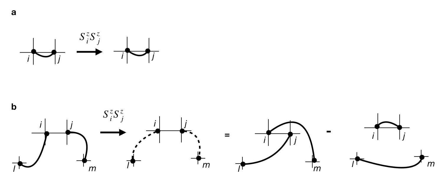
Figure 5: a) The action of the Ising part of $H_{ij}$ on a single bond $(i,j)$ leaves it invariant. b) The action of the Ising part of $H_{ij}$ on two bonds linked to $i$ and to $j$ converts them to singlet bonds (dashed lines), which can then be re-written as a sum of two tVB configurations.

If $(i,l)$ and $(j,m)$ are two triplet valence bonds from other sites $l$ and $m$ which terminate at $i$ and $j$ respectively, then

$$S^{z}_{i}S^{z}_{j}\ |(i,l)\rangle|(j,m)\rangle=\frac{1}{4}|[i,l]\rangle|[j,m]\rangle,$$ (15)

where we have employed the commutator notation $|[i,j]\rangle\equiv(|\uparrow\rangle_{i}|\downarrow\rangle_{j}-|\downarrow\rangle_{i}|\uparrow\rangle_{j})/\sqrt{2}$ to describe singlet RVBs. At first sight, this implies that the Ising terms will lead to a mixture of singlet and triplet bonds. However, the overcompleteness of the RVB representation, allows us to represent these two singlet bonds as a superposition of triplet bonds (see Fig. 5b). Direct algebraic expansion confirms that

$$|[1,2][3,4]\rangle=\left|(1,4)\right\rangle\left|(2,3)\right\rangle-\left|(1,3)\right\rangle\left|(2,4)\right\rangle.$$ (16)

which guarantees that the tRVB manifold of states that is closed under the time-evolution.

II Symmetry constraints on $\rm\bf t$RVB and impurity scattering

One of the key aspects of the tRVB theory, is the ability of local triplet pairs, formed within an atom, to escape and form a coherent condensate on the Fermi surface. Here we illustrate how the constraints of inversion symmetry in the FeSC allow this process to take place.

From Eq. (8) of the main text, the tRVB BCS Hamiltonian is

$$H=H_{\rm kin}+H_{P}=\sum_{\bf k}\tilde{\psi}_{\bf k}^{\dagger}\left[H_{\rm kin}({\bf k})\tau_{3}+\Delta_{ab}L_{a}\sigma_{b}\tau_{1}\right]\tilde{\psi}_{\bf k}.$$ (17)

where the sum is over half the Brillouin zone, to avoid double-counting. Following the notation of the main text, we denote the multi-orbital Bloch wavefunctions by $\vec{u}_{n,{\bf k}}$, which are the eigenstates of the tight-binding Hamiltonian, $H_{\rm kin}({\bf{k}})\vec{u}_{n,{\bf k}}=\epsilon_{n}({\bf k})\vec{u}_{n,{\bf k}}$. As we show in (II.1) the band diagonal pairing matrix elements of the superconducting gap are then related to the eigenvectors $\vec{u}_{n,{\bf k}}$ according to

$$\langle 0|H_{P}|n,-{\bf{k}},\alpha;n{\bf{k}}\beta\rangle=\vec{d}_{n}({\bf{k}})\cdot(-i\sigma_{2}\vec{\sigma})_{\alpha\beta}.$$ (18)

Here $|n,-{\bf{k}},\alpha;n{\bf{k}}\beta\rangle=a^{\dagger}_{n{\bf{k}}\beta}a^{\dagger}_{n,-{\bf{k}}\alpha}|0\rangle$ is a triplet pair of electrons in the n-th band and the d-vector

$$\vec{d}_{n}({\bf{k}})=-\vec{d}_{n}(-{\bf{k}})=i(\vec{u}_{n,{\bf{k}}}\times\vec{u}_{n,-{\bf{k}}})\cdot\underline{\Delta},$$ (19)

where $[\underline{\Delta}]_{ab}=\Delta_{ab}$ is the onsite gap function.

A finite magnitude of the vector $\vec{u}_{n,{\bf{k}}}\times\vec{u}_{n,-{\bf{k}}}$ plays a crucial role, for it allows the onsite pairing to migrate to the Fermi surface, giving rise to a gap $\Delta_{n}({\bf{k}})\sim|\vec{d}_{n}({\bf{k}})|$ that grows linearly with the order parameter $\underline{\Delta}$. Moreover, the linear growth of the Fermi surface gap with the order parameter guarantees that the pair susceptibility will acquire a logarithmic divergence in temperature, driving a Cooper instability at arbitrarily weak coupling. Conversely, if $\vec{u}_{n,{\bf{k}}}\times\vec{u}_{n,-{\bf{k}}}=0$ is zero, the pairing is entirely inter-band in character, there is no weak-coupling instability and the superconducting gap does not grow linearly with the order parameter.

In section (II.2) we discuss the conditions under which $\vec{u}_{n,{\bf{k}}}\times\vec{u}_{n,-{\bf{k}}}$ is finite.

II.1 Derivation of the matrix element

The pairing component of the Hamiltonian can be written out as

$$H_{P}=\sum_{{\bf{k}}}\left[\Delta_{ab}\bar{\psi}_{-{\bf{k}}}^{T}(L_{a}\sigma_{b})\psi_{{\bf{k}}}+{\rm H.c}\right],$$ (20)

where band and spin indices denoted $\bar{\psi}_{-{\bf{k}}}^{T}=\psi^{T}_{-{\bf{k}}}(-i\sigma_{2})$. To transform this into the band-basis, we note that the components of $\vec{u}_{n,{\bf{k}}}$ can be written in Dirac notation as the overlap between the orbital and band bases $(\vec{u}_{n,{\bf{k}}})^{\alpha}=\langle{\bf{k}}\alpha|n{\bf{k}}\rangle$, where $\alpha$ is the orbital index, and $n$ the band index. Now using completeness, the relationship between “bras” in the two bases is $\langle{\bf{k}}\alpha|=\sum_{n}\langle{\bf{k}}\alpha|n{\bf{k}}\rangle\langle n{\bf{k}}|$, and since destruction operators transform like “bra”s, it follows that $\psi_{{\bf{k}}a}=\sum_{n}\langle{\bf{k}}\alpha|n{\bf{k}}\rangle a_{n{\bf{k}}}$, or in terms of $\vec{u}_{n,{\bf{k}}}$ and band annihilation operator $a_{n\bf k}$,

$$\psi_{{\bf{k}}}=\sum_{n}\vec{u}_{n,{\bf{k}}}a_{n{\bf{k}}},\qquad\bar{\psi}^{T}_{-{\bf{k}}}=\sum_{n}\vec{u}^{T}_{n,{\bf{k}}}\bar{a}^{T}_{n,-{\bf{k}}},$$ (21)

where $\bar{a}^{T}_{n,-{\bf{k}}}=a^{T}_{n,-{\bf{k}}}(-i\sigma_{2})$. Using these relationships, we can re-write the pairing term in the band-basis as

$$H_{P} = \sum_{{\bf{k}},a,b,m,n}\left[\Delta_{ab}(\vec{u}^{T}_{m{\bf{k}}}L_{a}\vec{u}_{n,{\bf{k}}})\bar{a}^{T}_{m,-{\bf{k}}}\sigma_{b}a_{n{\bf{k}}}+{\rm H.c}\right]$$ (22)

$$= \sum_{{\bf{k}},m,n}\left[\bar{a}^{T}_{m,-{\bf{k}}}(\vec{d}_{mn}({\bf{k}})\cdot\vec{\sigma})a_{n,{\bf{k}}}+{\rm H.c}\right],$$ (23)

where the d-vector

$$[d_{mn}({\bf{k}})]_{b}=\sum_{a}(\vec{u}^{T}_{m{\bf{k}}}L_{a}\vec{u}_{n,{\bf{k}}})\Delta_{ab}.$$ (24)

Now since $[L_{a}]_{bc}=-i\epsilon_{abc}$, it follows that

$$(\vec{d}_{mn}({\bf{k}}))_{b}=-i(\vec{u}_{m,-{\bf{k}}}\times\vec{u}_{n,{\bf{k}}})_{a}\Delta_{ab}\equiv\left[-i(\vec{u}_{m,-{\bf{k}}}\times\vec{u}_{n,{\bf{k}}})\cdot\underline{\Delta}\right]_{b},$$ (25)

where we have used a matrix notation to write $\underline{\Delta}_{ab}\equiv\Delta$. The ability of local pairs to migrate onto the Fermi surface depends on the band-diagonal component of this matrix element,

$$\vec{d}_{n}({\bf{k}})=i(\vec{u}_{n,{\bf{k}}}\times\vec{u}_{n,-{\bf{k}}})\cdot\underline{\Delta},$$ (26)

where we have denoted $\vec{d}_{n}({\bf{k}})\equiv\vec{d}_{nn}({\bf{k}})$. Notice that because the cross-product is antisymmetric, the diagonal d-vector is odd parity in momentum, $\vec{d}_{n}({\bf{k}})=i(\vec{u}_{n,-{\bf{k}}}\times\vec{u}_{n,{\bf{k}}})\cdot\underline{\Delta}=-i(\vec{u}_{n,{\bf{k}}}\times\vec{u}_{n,-{\bf{k}}})\cdot\underline{\Delta}=-\vec{d}({\bf{k}})$.

Let us now compute the the amplitude to destroy a triplet Cooper pair out of the vacuum, $\langle 0|H_{P}|n,-{\bf{k}},\alpha;n,{\bf{k}}\beta\rangle$, where where $|n,-{\bf{k}},\alpha;n,{\bf{k}}\beta\rangle=a^{\dagger}_{n{\bf{k}}\beta}a^{\dagger}_{n,-{\bf{k}}\alpha}|0\rangle$. Substituting this into Eq(22) and explicitly exposing the spin indices, we obtain

$$\langle 0|H_{P}|n,-{\bf{k}},\alpha;n{\bf{k}}\beta\rangle = \langle 0|H_{P}a^{\dagger}_{n{\bf{k}}\beta}a^{\dagger}_{n-{\bf{k}}\alpha}|0\rangle$$ (27)

$$= \sum_{l,m,\gamma,\delta}\langle 0|a_{l,-{\bf{k}}\gamma}\left(\vec{d}_{lm}({\bf{k}})\cdot(-i\sigma_{2}\vec{\sigma})_{\gamma\delta}\right)a_{m{\bf{k}}\delta}a^{\dagger}_{n{\bf{k}}\beta}a^{\dagger}_{n-{\bf{k}}\alpha}|0\rangle$$ (28)

$$= \vec{d}_{nn}({\bf{k}})\cdot(-i\sigma_{2}\vec{\sigma})_{\alpha\beta}$$ (29)

$$\equiv \vec{d}_{n}({\bf{k}})\cdot(-i\sigma_{2}\vec{\sigma})_{\alpha\beta}.$$ (30)

II.2 Conditions for a finite gap

As a second step we discuss the symmetry enforced properties of $\vec{u}_{n,\bf k}$ in our two dimensional model of FeSe, identifying the non-trivial representation of the two-dimensional inversion symmetry, resulting from the non-symmorphic crystal structure as an origin of the finite Fermi surface support of the gap. The two-dimensional inversion symmetry, according to which, $H_{\rm kin}({\bf k})=M^{-1}H_{\rm kin}(-{\bf k})M$ ($M$ is unitary), implies that $\vec{u}_{n,-{\bf k}}=M\vec{u}_{n,\bf k},$. Thus if the representation of inversion symmetry is trivial, so that $M=\mathbf{1}$ the Fermi surface d-vector vanishes

$$\vec{d}_{n}({\bf{k}})=i(\vec{u}_{n,{\bf{k}}}\times\vec{u}_{n,{\bf{k}}})\cdot\underline{\Delta}=0,$$ (31)

so that the onsite triplet pairing does not escape to the Fermi surface. This is the essence of the observations by Anderson Anderson (1985), Hotta and Ueda Hotta and Ueda (2004).

For the specific case of the layered iron-based superconductors, treated in a 2D model of a single plane, the three $t_{2g}$ orbitals $\left|xz\right\rangle$, $\left|yz\right\rangle$ and $\left|xy\right\rangle$ transform differently under the 2D inversion operation, $(x,y,z)\to(-x,-y,z)$, which results in a non-trivial representation $M=(-1,-1,1)$ of the 2D inversion. As a result, even in presence of time-reversal symmetry (which implies $\vec{u}_{n,-{\bf{k}}}=\vec{u}_{n,{\bf{k}}}^{*}$) the components of $\vec{u}_{n,\bf k}$ cannot all be real, resulting in a non-zero $\vec{d}$ vector,

$$\vec{u}_{n,\bf k}=M\vec{u}^{*}_{n,\bf k}\Rightarrow\vec{u}_{n,{\bf k}}=\left(\begin{array}[]{cc}iu_{n,xz}\\ iu_{n,yz}\\ u_{n,xy}\end{array}\right).$$ (32)

For the case $\Delta_{ab}=\Delta{\rm diag}(1,1,-2)$ considered in the paper,

$$\vec{d}_{n}({\bf k})=\Delta u_{n,xy}\left(\begin{array}[]{cc}-u_{n,yz}\\ u_{n,xz}\\ 0\end{array}\right).$$ (33)

Note that the $\vec{d}$ vector is in the x-y plane and its value crucially depends on the $xy$ orbital admixture of the electrons at the Fermi surface. In other words, if the $xy$ orbital is localized there will be no triplet superconductivity.

II.3 Robustness against disorder

A question which is related to the symmetries of the superconducting gap regards the stability of $T_{c}$ against the inclusion of scalar impurities. In this section we outline a comparison of usual $s$-wave, usual $p$-wave, $s_{+-}$ and tRVB pairing and loosely follow the textbook Abrikosov et al. (2012). We consider a multiorbital superconductor, which in the clean limit has Nambu-Gor’kov Green’s function

$$\mathcal{G}(i\nu,{\bf k})=[i\nu-\mathcal{H}({\bf k})]^{-1}.$$ (34)

Figure 6: Resummation of impurity scattering in non-crossing approximation using Nambu matrix Green’s functions.

Here, $\mathcal{H}({\bf k})=H_{\rm kin}({\bf{k}})\tau_{3}+\hat{\Delta}({\bf k})\tau_{1}$, where $\hat{\Delta}({\bf k})$ is a matrix in spin and orbital space, e.g. $\hat{\Delta}({\bf k})=\sum_{a,b}\Delta_{ab}L_{a}\sigma_{b}$ in the tRVB case, $\hat{\Delta}({\bf k})=\Delta\cos(k_{1})\cos(k_{2})$ for $s_{\pm}$ pairing and $\hat{\Delta}({\bf k})=\Delta\sum_{a=1,2}\sin(k_{a})\sigma_{a}$ for ordinary $p$-wave superconductors. The diagrammatic, non-crossing resummation of impurity lines, Fig. 6, of point like scatterers of strength $u_{0}$ and density $n_{\rm imp}$ leads to

$$[\mathcal{G}^{-1}(i\nu,{\bf k})-\Sigma(i\nu,{\bf k})]\boldsymbol{\mathcal{G}}(i\nu,{\bf k}) = \mathbf{1},$$ (35)

$$\Sigma(i\nu,{\bf k}) = n_{\rm imp}u_{0}^{2}\int_{\bf p}\tau_{3}\boldsymbol{\mathcal{G}}(i\nu,{\bf p})\tau_{3}.$$ (36)

We use the notation $\int_{\bf p}=\int\frac{d^{d}p}{(2\pi)^{d}}$. To establish the stability of the superconductivity against disorder, we need to investigate the persistance of the Cooper instability. Since this is an intraband phenomenon we consider the coupled equations

$$[\mathcal{G}_{n}^{-1}(i\nu,{\bf k})-\Sigma_{n}(i\nu,{\bf k})]\boldsymbol{\mathcal{G}}_{n}(i\nu,{\bf k}) = \mathbf{1},$$ (37)

$$\Sigma_{n}(i\nu,{\bf k}) = n_{\rm imp}u_{0}^{2}\sum_{m}\int_{\bf p}|\langle{u_{n,{\bf k}}|u_{m,{\bf p}}}\rangle|^{2}\tau_{3}\boldsymbol{\mathcal{G}}_{m}(i\nu,{\bf p})\tau_{3},$$ (38)

where $\mathcal{G}_{n}(i\nu,{\bf k})=[i\nu-\epsilon_{n}({\bf k})\tau_{3}-\Delta_{n}({\bf k})\tau_{1}]^{-1}$ and $\Delta_{n}({\bf k})=\langle{u_{n,{\bf k}}|\hat{\Delta}({\bf k})|u_{n,{\bf k}}}\rangle$, i.e. only the intra-band part of the pairing is kept. For orbital independent superconducting order parameters (e.g. ordinary s-wave), these expressions are exact. We will use the following matrix form

$$\Sigma_{n}(i\nu,{\bf k})=\left(\begin{array}[]{cc}\Sigma^{N}_{n}(i\nu,{\bf k})&\Sigma^{A}_{n}(i\nu,{\bf k})\\ {[\Sigma^{A}_{n}(i\nu,{\bf k})]}^{\dagger}&-\Sigma^{N}_{n}(-i\nu,{\bf k})\end{array}\right).$$ (41)

Now, following Abrikosov and Gor’kov, we seek a self-consistent solution using the low-frequency ansatz $\Sigma_{n}^{N}(i\nu,{\bf k})=\tilde{\Sigma}_{n}^{N}({\bf k})-i\nu\Gamma_{\nu,n}({\bf k})$ and $\Sigma_{n}^{A}(i\nu,{\bf k})=-\Delta_{n}({\bf k})\tilde{\Gamma}_{\nu,n}({\bf k})$, which can be justified a posteriori. Both self-energies are only weakly momentum dependent in the cases of interest. As usual Abrikosov et al. (2012), the frequency independent part $\tilde{\Sigma}_{n}^{N}({\bf k})$ is absorbed into a renormalization of dispersion, chemical potential and crystal field and omitted from further considerations. Then, $\boldsymbol{\mathcal{G}}_{n}(i\nu,{\bf k})=[i\bar{\nu}_{n}-\epsilon_{n}({\bf k})\tau_{3}-\bar{\Delta}_{n}({\bf k})\tau_{1}]^{-1}$ with $i\bar{\nu}_{n}=i\nu(1+\Gamma_{\nu,n}({\bf k}))$ and $\bar{\Delta}_{n}=\Delta_{n}(1+\tilde{\Gamma}_{\nu,n}({\bf k}))$, where $1+\Gamma_{\nu,n}({\bf k})=Z^{-1}_{\nu,n}({\bf k})$ corresponds to the wavefunction renormalization of the Green’s function, while $\tilde{\Gamma}_{\nu,n}({\bf k})$ is the impurity correction to the pairing vertex.

The BCS equation of impure superconductors with $\hat{\Delta}({\bf k})=f({\bf k})\hat{\Delta}$, where $f({\bf k})$ is a normalized form factor, is

$$\frac{\hat{\Delta}}{g}=-T\sum_{\nu}\int_{\bf k}f({\bf k})\mathbf{F}(i\nu,{\bf k})\simeq T\sum_{\nu,n}\rho_{n}(E_{F})\Big{\langle}\left|u_{n,{\bf k}}\right\rangle\frac{f({\bf k})\bar{\Delta}_{n}({\bf k})}{\sqrt{\bar{\nu}^{2}+\bar{\Delta}_{n}({\bf k})^{2}}}\left\langle u_{n,{\bf k}}\right|\Big{\rangle}_{\rm FS},$$ (42)

where $\langle\dots\rangle_{\rm FS}$ denotes the angular Fermi surface average and ${\mathbf{F}}(i\nu,{\bf k})$ denotes the anomalous Green’s function. If ${\Gamma}_{\nu,n}({\bf k})=\tilde{\Gamma}_{\nu,n}({\bf k})$, as it occurs in the simplest s-wave case, self-energy and vertex correction cancel in numerator and denominator of Eq. (42) and $T_{c}$ is unchanged (“Anderson’s theorem”). In contrast, for $s_{\pm}$ pairing, $\tilde{\Gamma}_{\nu,n}({\bf k})\ll\Gamma_{\nu,n}({\bf k})$ due to partial cancellation of contributions from electron and hole pockets in the anomalous self energy. Even more drastically, for ordinary single band p-wave triplet pairing, where $f({\bf k})=\sum_{a=1,2}\sin(k_{a})\sigma_{a}$ is a matrix in spin space, $\tilde{\Gamma}_{\nu,n}({\bf k})=0$ due to the symmetries of the order parameter. Therefore, p-wave pairing is very susceptible to the presence of scalar impurities.

We now demonstrate that $\tilde{\Gamma}_{\nu n}({\bf k})>0$ for tRVB in iron based superconductors, despite the fact that the tRVB state is effectively p-wave on the Fermi surface. The self-consistent condition for the anomalous self-energy, Eq. (38), can be written as

$${\Delta_{n}({\bf k})}\tilde{\Gamma}_{\nu,n}({\bf k}) = -n_{\rm imp}{u_{0}^{2}}\langle u_{n,{\bf k}}|\Big{[}\int_{\bf p}{\bf F}(i\nu,{\bf p})\Big{]}|u_{n,{\bf k}}\rangle$$ (43)

Therefore, a non-zero $\tilde{\Gamma}_{\nu,n}({\bf k})$ requires an onsite pairing amplitude, which is indeed a crucial aspect of tRVB theory. For illustration, we consider the simplest tRVB state $\hat{\Delta}=\Delta\sum_{a=1,2}L_{a}\sigma_{a}$. For this choice $\int_{\bf p}{\mathbf{F}}(i\nu,{\bf p})\propto-\hat{\Delta}$ (keeping only intraband pairing) such that the matrix structure of Eq. (42) is indeed fulfilled in the leading logarithm approximation. We therefore find a momentum independent vertex correction which obeys

$$\tilde{\Gamma}_{\nu,n}=n_{\rm imp}u_{0}^{2}\sum_{m}\int\frac{d^{d}p}{(2\pi)^{d}}\frac{|\vec{d}_{m}({\bf p})|^{2}(1+\tilde{\Gamma}_{\nu,m})/(2\Delta^{2})}{\bar{\nu}_{n}^{2}+\epsilon_{m}({\bf p})^{2}+|\vec{d}_{m}({\bf p})|^{2}(1+\tilde{\Gamma}_{\nu,m})^{2}}>0.$$ (44)

The finiteness of this quantity reflects the local character of the tRVB pairing, and it is this feature that guarantees partial protection with respect to elastic scattering.

III Observables in iron based superconductors

For the BdG Hamiltonian $\mathcal{H}({\bf k})=H_{\rm kin}({\bf{k}})\tau_{3}+\Delta_{ab}L_{a}\sigma_{b}\tau_{1}$ the Matsubara Green’s function can be expressed as

$$\mathcal{G}(i\epsilon_{n},{\bf k})\equiv[i\epsilon_{n}-\mathcal{H}({\bf k})]^{-1}.$$ (45)

In this section we concentrate on intraband pairing, use the notation $\Delta_{n}({\bf k})=\vec{d}_{nn}({\bf k})\cdot\vec{\sigma}+d^{(0)}_{nn}({\bf k})$ and the multi index $(n,h)$, e.g. in the energy $E_{n,h}({\bf k})=\sqrt{\xi_{n}^{2}+(d_{nn}^{(0)}+hd_{nn})^{2}}$ (the quantum number $h=\pm 1$ denotes the eigenvalues $hd_{nn}$ of $\vec{d}_{nn}\cdot\vec{\sigma}$ and $\xi_{n}({\bf{k}})$ is the dispersion in band $n$). For pure singlet or pure triplet states, $E_{n,h}({\bf k})=E_{n,-h}({\bf k})$ and we can suppress the index $h$. All observables in this section are computed for the tight-binding model of Ref. Daghofer et al. (2010) and a gap function $\Delta(L_{1}\sigma_{1}+L_{2}\sigma_{2}-2L_{3}\sigma_{3})$. The sign structure of the $\vec{d}$ vector on the Fermi surfaces of this tight binding model is summarized in Fig. 7.

Figure 7: Illustration of signs (red/blue color) of the components of d-vectors on the Fermi surfaces in the absence of SOC. Note that the $d_{x}$ ($d_{y}$) components approximately vanish on the $Y$ ($X$) electron pocket. The component $d_{z}=0$ by symmetry.

III.1 Local density of states and QPI

The even and odd frequency parts of the impurity contribution Maltseva and Coleman (2009) to the local DOS in Fourier space $\delta\rho^{e/o}({\bf q},z)=V({\bf q})\Lambda^{e/o}({\bf q},z)$ are

$$\Lambda^{e/o}({\bf q},z) = \frac{1}{2\pi}\text{Im}\int_{{\bf k}}{\hbox{Tr}}\left\{\left(\begin{array}[]{c}1\\ \tau_{3}\end{array}\right)\mathcal{G}^{A}({\bf k}_{+},z)\tau_{3}\mathcal{G}^{A}({\bf k},z)\right\}$$ (49)

$$\simeq \frac{2}{\pi}\sum_{n,m}\text{Im}\int_{\bf k}\frac{|\left\langle{n,{\bf k}_{+}}|{m,{\bf k}}\right\rangle|^{2}}{[z^{2}-E_{n}({\bf k}_{+})^{2}][z^{2}-E_{m}({\bf k})^{2}]}$$

$$\times\begin{cases}z(\xi_{n}({\bf k}_{+})+\xi_{m}({\bf k})),&\text{ for }\Lambda^{e}({\bf q},z),\\ z^{2}+\xi_{n}({\bf k}_{+})\xi_{m}({\bf k})-\vec{d}_{nn}({\bf k}_{+})\cdot\vec{d}_{mm}({\bf k}),&\text{ for }\Lambda^{o}({\bf q},z),\end{cases}$$

where ${\bf k}_{+}={\bf k}+{\bf q}$. Here, we considered predominant intraband pairing and the case of absent singlet pairing ($d_{nn}^{(0)}=0$). In the reverse case of absent triplet pairing ($\vec{d}_{nn}=0$), but present singlet pairing ($d_{nn}^{(0)}\neq 0$) we obtain the analogous result, i.e. Eq. (49) with the replacement $\vec{d}_{nn}({\bf k}_{+})\cdot\vec{d}_{mm}({\bf k})\rightarrow d_{nn}^{(0)}({\bf k}_{+})d_{mm}^{(0)}({\bf k})$. At the Fermi surface ($\xi_{n}({\bf k})=0$) this integral is dominated by momenta at where $E_{n}({\bf k}_{+})\equiv|\vec{d}_{n}({\bf k}_{+})|$ and $E_{m}({\bf k})\equiv|\vec{d}_{m}({\bf k})|$ are equal and by frequencies $z$ which are on-shell. In order to illustrate this dominant physics in the main text, we replace $z\rightarrow\sqrt{|\vec{d}_{n}({\bf k}_{+})||\vec{d}_{m}({\bf k})|}$, keeping in mind that the proper equation is Eq. (49).

When the STM bias voltage $eV$ is close to or below the superconducting gap, the sign of $\vec{d}_{nn}({\bf k}_{+})\cdot\vec{d}_{mm}({\bf k})$ (or $d_{nn}^{(0)}({\bf k}_{+})d_{mm}^{(0)}({\bf k})$ for the singlet case) in the numerator of Eq. (49) determines whether $\Lambda^{o}({\bf q},eV)$ is enhanced (negative sign) or suppressed (positive sign) at a certain wavevector ${\bf q}$ Hirschfeld et al. (2015). In particular, singlet $s_{\pm}$ pairing enhances $\Lambda^{o}({\bf q},eV+i0)$ at ${\bf q}\sim(\pi,0),(0,\pi)$ due to the relative sign $d_{nn}^{(0)}({\bf k}_{+})d_{mm}^{(0)}({\bf k})<0$ of the pairing gap between electron and hole pockets. Our results for the triplet case, Eq. (49), and the predominantly sign changing structure of d-vectors between electron and hole pockets, Fig. 7, demonstrate that the interorbital triplet pairing $\Delta(\vec{L}_{\perp}\cdot\vec{\sigma}_{\perp})=\Delta(L_{1}\sigma_{1}+L_{2}\sigma_{2})$ may have a qualitatively similar effect as $s_{\pm}$ singlet pairing.

III.2 Spin susceptibility: Knight shift and spin resonance

The correlation function of two operators $\hat{O}$ and $\hat{O}^{\prime}$ is ($\epsilon_{n}^{+}=\epsilon_{n}+\omega_{m}$)

$$\chi_{OO^{\prime}}({\bf q},i\omega_{m}) = -\frac{1}{2}T\sum_{\epsilon_{n}}\int_{\bf k}{\hbox{Tr}}[\hat{O}\mathcal{G}(i\epsilon_{n}^{+},{\bf k}^{+})\hat{O}^{\prime}\mathcal{G}(i\epsilon_{n},{\bf k})]$$ (50)

For approximately spherical Fermi surfaces $\xi_{n}({\bf k})=\xi_{n}(k)$ and predominant intraband pairing this leads to the static spin susceptibility Mineev and Samokhin (1999)

$${\chi_{S_{\mu},S_{\nu}}^{R}(0,0)=\sum_{n}\frac{\nu_{n}(E_{F})}{2}\left\langle\hat{d}_{nn}^{(\mu)}\hat{d}_{nn}^{(\nu)}Y(\hat{k},T)+[\delta_{\mu\nu}-\hat{d}_{nn}^{(\mu)}\hat{d}_{nn}^{(\nu)}]\right\rangle_{\rm FS(n)}}$$ (51)

where $Y(\hat{k},T)=\int d\xi\;{1}/({4T\cosh^{2}(E/2T)})$

In the limit of small $\Delta$ and no spin-orbit coupling, where Eq. (51) is valid, the intra-band $\vec{d}$-vector on the Fermi surface is in the plane. This means that for superconductors with small gap the change in the spin contribution to the Knight shift will be only in the plane. On the other hand, when the gap size is comparable to the inter-band splitting, local inter-band contributions become important and the change in the Knight shift becomes purely in the $z$-direction. Therefore, the $L_{1}\sigma_{1}+L_{2}\sigma_{2}-2L_{3}\sigma_{3}$ pairing can predict different Knight shifts but it is almost always aniostropic.

We now switch to the discussion of the spin resonance and the finite $\bf q$, $\Omega$ response. For purely spin singlet or purely spin triplet pairing we obtain

$$\chi_{S_{\mu},S_{\nu}}^{R}({\bf q},\Omega) = \frac{1}{4}\sum_{n,m}\sum_{hh^{\prime}}\int_{\bf k}|\left\langle{n,{\bf k}}|{m,{\bf k^{+}}}\right\rangle|^{2}$$ (52)

$$\Big{[}\left(\frac{\tanh\left(\frac{E_{n}({\bf k})}{2T}\right)-\tanh\left(\frac{E_{m}({\bf k^{+}})}{2T}\right)}{E_{n}({\bf k})-E_{m}({\bf k^{+}})+\Omega^{+}}+\Omega\rightarrow-\Omega\right)$$

$$\times\left(M_{\mu\nu}^{hh^{\prime}}(u_{n,h,{\bf k}}u_{m,h^{\prime},{\bf k}^{+}}+v_{n,h,{\bf k}}v_{m,h^{\prime},{\bf k}^{+}})^{2}\right)$$

$$+\left(\frac{\tanh\left(\frac{E_{n}({\bf k})}{2T}\right)+\tanh\left(\frac{E_{m}({\bf k^{+}})}{2T}\right)}{E_{n}({\bf k})+E_{m}({\bf k^{+}})+\Omega^{+}}+\Omega\rightarrow-\Omega\right)$$

$$\times\left(M_{\mu\nu}^{hh^{\prime}}(u_{n,h,{\bf k}}v_{m,h^{\prime},{\bf k}^{+}}-v_{n,h,{\bf k}}u_{m,h^{\prime},{\bf k}^{+}})^{2}\right)\Big{]}.$$

We have introduced the matrix elements of spin-operators

$$M_{\mu\nu}^{hh^{\prime}} = \frac{1}{8}\Big{\{}[1-hh^{\prime}](\delta_{\mu\nu}-\hat{d}_{(\mu}({\bf k})\hat{d}_{\nu)}({\bf k}^{+}))+[1+hh^{\prime}]\hat{d}_{(\mu}({\bf k})\hat{d}_{\nu)}({\bf k}^{+})$$ (53)

$$+i\epsilon_{\mu\nu\rho}(h\hat{d}_{\rho}({\bf k})-h^{\prime}\hat{d}_{\rho}({\bf k}^{+}))+hh^{\prime}\delta_{\mu\nu}(1-\hat{d}({\bf k})\cdot\hat{d}({\bf k}^{+}))\Big{\}},$$

and coherence factors

$$u_{n,h,{\bf{k}}}=\frac{\xi_{n}+E_{n}}{\sqrt{2E_{n}(\xi_{n}+E_{n})}},\quad v_{n,h,{\bf{k}}}=\frac{1}{\sqrt{2E_{n}(\xi_{n}+E_{n})}}\times\begin{cases}d^{(0)}_{nn},&\text{singlet,}\\ hd_{nn},&\text{triplet.}\end{cases}$$ (54)

The spin-resonance, as obtained by the pole of the RPA resummation of spin-interaction and bare $\chi_{S_{\mu}S_{\nu}}$ susceptibility, is most crucially determined by the last term (we omit the index $h$ in coherence factors)

$$\sum_{hh^{\prime}}M_{\mu\nu}^{hh^{\prime}}(u_{n,h,{\bf k}}v_{m,h^{\prime},{\bf k}^{+}}-v_{n,h,{\bf k}}u_{m,h^{\prime},{\bf k}^{+}})^{2}\stackrel{{\scriptstyle\text{singlet}}}{{=}}\frac{\delta_{\mu\nu}}{2}(u_{n,{\bf k}}v_{m,{\bf k}^{+}}-v_{n,{\bf k}}u_{m,{\bf k}^{+}})^{2}.$$ (55)

In the case of singlet pairing, it approximately vanishes unless $v_{m,{\bf k}^{+}}v_{m,{\bf k}}<0$, i.e. when $\Delta_{m,{\bf k}^{+}}\Delta_{m,{\bf k}}<0$ (we have omitted $h$ from the coherence factors since they are not $h$ dependent in the singlet case). In particular, the spin resonance is absent for $s_{++}$ pairing, while it may occur for ${\bf q}$ connecting electron and hole pockets for $s_{\pm}$. Analogously, for the triplet case

$$\sum_{hh^{\prime}}M_{\mu\nu}^{hh^{\prime}}(u_{n,h,{\bf k}}v_{m,h^{\prime},{\bf k}^{+}}-v_{n,h,{\bf k}}u_{m,h^{\prime},{\bf k}^{+}})^{2} \stackrel{{\scriptstyle\text{triplet}}}{{=}} \frac{\delta_{\mu\nu}}{2}(u_{n,{\bf k}}v_{m,{\bf k}^{+}}\hat{d}_{mm}({\bf k}^{+})+v_{n,{\bf k}}u_{m,{\bf k}^{+}}\hat{d}_{nn}({\bf k}))^{2}$$ (56)

$$-2u_{n,{\bf k}}v_{m,{\bf k}^{+}}v_{n,{\bf k}}u_{m,{\bf k}^{+}}\hat{d}_{nn}^{(\nu}({\bf k})\hat{d}_{mm}^{\mu)}({\bf k}^{+}).$$

Here, $v_{m,{\bf k}}=v_{m,h=+,{\bf k}}$ and similarly for $u_{m,{\bf k}}$. Clearly, a sharp spin-resonance can only appear upon inclusion of SOC (and the generation of a full gap in the electronic spectrum). At the same time, the relative signs of $\vec{d}$-vectors, Fig. 7, demonstrates that the coherence factors [more precisely the matrix elements in Eq. (56)] are typically non-vanishing and positive, for relative momenta connecting electron and hole pockets. This is consistent with a spin resonance at ${\bf q}=(0,\pi);(\pi,0)$.

III.3 Josephson scanning tunneling microscopy

In this section we present details on Josephson scanning tunneling microscopy.

III.3.1 Hamiltonian of a single Josephson junction

The Josephson Hamiltonian describing a single tunnel junction is

$$\mathcal{H}_{\rm Jos}=-E_{C}\frac{\partial^{2}}{\partial\phi^{2}}-E_{J}\cos(\phi-\phi_{0}),$$ (57)

where $\phi$ is the current induced phase difference between tip and junction, $\phi_{0}$ a phase offset, $E_{C}$ the charging energy and the Josephson energy is $E_{J}=|I_{J}|\frac{\hbar}{e}$ ($I_{J}$ is the associated Josephson current), where microscopically

$${I_{J}({\bf x}_{0})=2\frac{e}{\hbar}\int(dE)n_{F}(E)\text{Im}\left\{{\hbox{Tr}}^{\sigma}\left[F_{\rm tip}^{(nn^{\prime})}(E^{+};{\bf x}_{0},{\bf x}_{0})t^{n^{\prime}m}F_{\rm sample}^{(mm^{\prime})}(E^{+};{\bf x}_{0},{\bf x}_{0})t^{m^{\prime}n,*}\right]\right\}}.$$ (58)

Here, Einstein summations are assumed and $t^{mn}$ is the orbital ($m,n$) dependent tunneling element with tip position ${\bf x}_{0}$. We consider an STM tip made from the same tRVB material as the probe. In this case, $I_{J}({\bf x}_{0})$ is non-zero, real, and, for a perfectly staggered order parameter, $\phi_{0}$ is position dependent $\phi_{0}({\bf x})=\text{arg}[(-1)^{x+y}]$

III.3.2 Experimental design

Here we design a measurement which measures $\phi_{0}({\bf x})$ in Eq. (57). In order to ensure a coherent phase difference between sample and tip, we propose an experiment with two coherently coupled tips which form a SQUID. A simple setup is a double tip made from a single superconducting material. The staggered superconducting gap can be observed as the structure is rotated (one tip is stationary and encircled by the other), Fig. 8 a.

For an experiment which probes the phase difference between sample and tip, $E_{C}$ should be smaller than $E_{J}$. The capacitance and tunnel coupling of a superconducting tip with atomic resultion imply, however, the reverse regime $E_{C}\gg E_{J}$. Therefore, to ensure phase coherent tunneling, we propose the inclusion of a large shunt capacitor, such that $E_{C}\sim{e^{2}}/({C_{\rm tip}+C_{\rm shunt}})\ll E_{J}$, see Fig. 8 a.

III.3.3 Experimental protocol

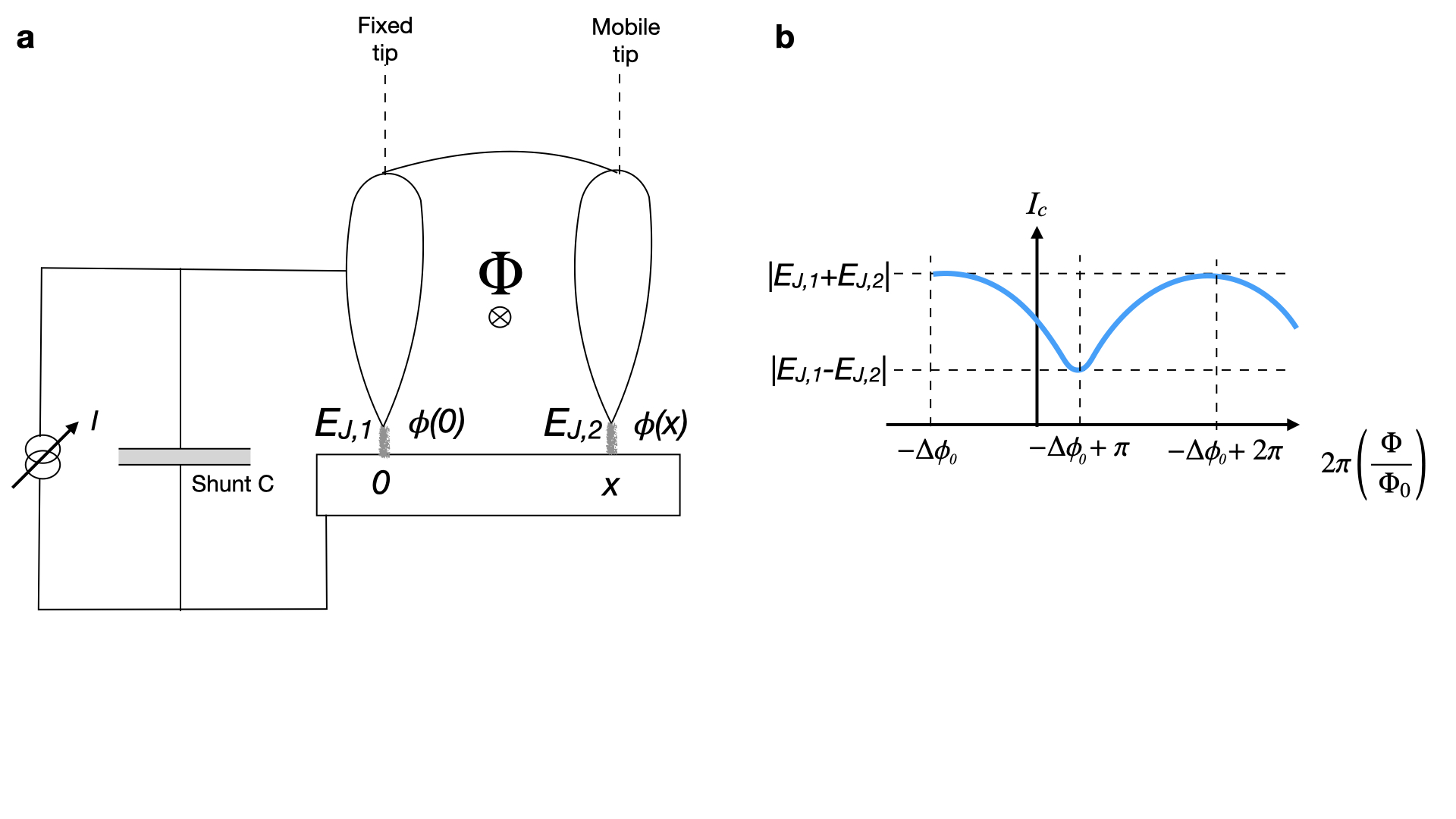
Figure 8: a SQUID geometry of the proposed Josephson tunneling microscopy, including the shunt capacitor C, b critical current as a function of applied flux $\Phi$, where $\Delta\phi_{0}=\phi_{0}({\bf x}_{1})-\phi_{0}({\bf x}_{2})$.

In summary, the effective Hamiltonian for the setup presented in Fig. 8 a is

$$\mathcal{H}_{\rm SQUID}=-\text{Re}\left[e^{i\phi}\left(E_{J,1}+E_{J,2}e^{i\alpha}\right)\right],$$ (59)

with $\phi=\Delta\phi-\frac{2e}{\hbar}A_{1}L_{1}+\phi_{0}({\bf x}_{1}),\alpha=\frac{2\pi\Phi}{\Phi_{0}}+\phi_{0}({\bf x}_{2})-\phi_{0}({\bf x}_{1})$. The critical current of the (generically asymmetric) SQUID is

$$I_{c}=\frac{2e}{\hbar}\sqrt{E_{J,1}^{2}+E_{J,2}^{2}+2E_{J,1}E_{J,2}\cos\left(\frac{2\pi\Phi}{\Phi_{0}}+\phi_{0}({\bf x}_{1})-\phi_{0}({\bf x}_{2})\right)},$$ (60)

and presented in Fig. 8 b. The experimental protocol is then to determine for each pair of positions ${\bf x}_{1,2}$, whether the SQUID encloses a $\phi_{0}({\bf x}_{1})-\phi_{0}({\bf x}_{2})=\pi$ junction or an ordinary junction $\phi_{0}({\bf x}_{1})-\phi_{0}({\bf x}_{2})=0$. This is observed by $I_{c}$ being minimal or maximal at zero flux. In the tRVB scenario, we expect that the phase $e^{i[\phi_{0}({\bf x})-\phi_{0}({0})]}\sim(-1)^{x+y}$ alternates between neighboring plaquettes while for ordinary superconductors no such alternation will be observed.