Thermalization and its Breakdown for a Large Nonlinear Spin

Abstract

By developing a semi-classical analysis based on the Eigenstate Thermalization Hypothesis, we determine the long time behavior of a large spin evolving with a nonlinear Hamiltonian. Despite integrable classical dynamics, we find the Eigenstate Thermalization Hypothesis for the diagonal matrix elements of observables is satisfied in the majority of eigenstates, and thermalization of long time averaged observables is generic. The exception is a novel mechanism for the breakdown of thermalization based on an unstable fixed point in the classical dynamics. Using the semi-classical analysis we derive how the equilibrium values of observables encode properties of the initial state. This analysis shows an unusual memory effect in which the remembered initial state property is not conserved in the integrable classical dynamics. We conclude with a discussion of relevant experiments and the potential generality of this mechanism for long time memory and the breakdown of thermalization.

In recent years, experiments on ultra cold atoms and trapped ionsBloch et al. (2008); Ludlow et al. (2015); Shaffer et al. (2018); Zibold et al. (2010) have succeeded in producing quantum systems that, on relevant time scales, are completely isolated from an environment. Surprisingly, many of these experiments find long time behavior that mimics a system coupled to an environment. These experiments prompt the question of thermalization: Given an initial state $\left|\psi(t=0)\right>$, a Hamiltonian $H=\sum_{n}E_{n}\left|n\right>\left<n\right|$, and an observable $O$, when and why does the long time average of $O$:

$$O(t,T)=\frac{1}{T}\int_{t}^{t+T}d\tau\left<\psi(\tau)\right|O\left|\psi(\tau)\right>$$ (1)

lose memory of its initial state? In other words, when does $O(t,T)$, at long time $t$, depend only on the energy of the initial state?

The eigenstate thermalization hypothesis (ETH)Deutsch (1991); Srednicki (1994); Rigol et al. (2008); D’Alessio et al. (2016); Deutsch (2018); Jensen and Shankar (1985); Mori et al. (2018) attempts to answer this question. Briefly, it states that if A1) $\left<n\right|O\left|n\right>$ changes very little between eigenstates with similar energy; A2) the level spacings, $E_{n}-E_{n+1}$, are sufficiently small; and A3) the energy uncertainty of the initial state is sufficiently small, then an eigenstate, randomly selected from a micro-canonical ensemble at the energy of the initial state, will describe the long time average observable (LTO): $O(t,T)\approx\left<n\right|O\left|n\right>$ for large $t$ and $T$.

ETH was originally discussedDeutsch (1991); Srednicki (1994) in classically chaotic systems where the eigenstates behave similar to random matrices and allows one to hypothesize additional structure on the off diagonal matrix elements of observables, $\left<n\right|O\left|m\right>$. While this stronger version of ETH allows one to predict relaxation times and response functionsD’Alessio et al. (2016), we will focus on an integrable model and therefore restrict our attention to the weaker version presented above and questions regarding the memory apparent in long time averages.

In extended systems, the standard mechanism for the breakdown of thermalization is the emergence of an extensive set of conserved charges due to underlying integrabilityPolkovnikov et al. (2011); Batchelor and Foerster (2016); Cassidy et al. (2011) or a random disorder potentialImbrie et al. (2017); Nandkishore and Huse (2015); Abanin et al. (2019). In few mode bosonic systems, thermalization has been predicted from semi-classical chaosTikhonenkov et al. (2013); Arwas et al. (2015); Khripkov et al. (2016, 2018); Arwas and Cohen (2016, 2017, 2019); Pizzi et al. (2019a), and it was recently shown that thermalization could fail when an oscillatory drive produced a time crystalPizzi et al. (2019b).

In this article, we explore a similar phenomenon for the long time behavior of a quantum evolution, but for a system which is not extended nor classically chaotic. The model we study is that of an SU(2) spin with large fixed size $|J|>50$ and evolving with respect to the Hamiltonian

$$H=-J_{x}+\frac{\Lambda}{2|J|}J_{z}^{2},$$ (2)

where $J_{x},J_{z}$ and $J_{y}$ are the canonical SU(2) spin operators, and we assume $\Lambda>1$. We formulate the question of thermalization for this system by asking: 1) for which initial states do LTOs thermalize and approach a micro-canonical ensemble, and 2) for states that do not thermalize, what is the mechanism that maintains information about the initial state. We focus our analysis on the time averages, $T>>1$, of observables $O=J_{x}$ and $O=J_{z}$, but check by exact calculation that the results remain unchanged for $T\rightarrow 0$.

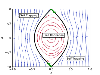
Figure 1: Classical trajectories: the separatrix is shown in black (bold) and separates the circular free-oscillation trajectories (red) from the self-trapping ones (blue). The red dots mark the unstable fixed point at $(z=0,\phi=\pm\pi)$ and the green arrows mark the unstable directions.

This spin Hamiltonian is expected to describe boson tunneling experimentsZibold et al. (2010); Strobel et al. (2014), and the theory community has explored its dynamicsRaghavan et al. (1999); Micheli et al. (2003); Mahmud et al. (2005); Chuchem et al. (2010); Huang et al. (2012); Lapert et al. (2012); Khripkov et al. (2013); Lovas et al. (2017); Mathew and Tiesinga (2017); Kelly et al. (2019); Hennig et al. (2012); Morita et al. (2006). While expressions for exact eigenstatesMorita et al. (2006) do not transparently answer the above questions, we find particularly useful a semi-classical analysisRaghavan et al. (1999); Micheli et al. (2003); Mahmud et al. (2005); Polkovnikov (2010); Chuchem et al. (2010); Khripkov et al. (2013); Lovas et al. (2017); Mathew and Tiesinga (2017); Mori (2017); Hennig et al. (2012) that describe the classical trajectories shown in Fig. 1. These trajectories, and corresponding eigenstates, have two distinct behaviors known as Josephson oscillation and self trapping, and are separated by a separatrix at $E=1$. Unlike the few-mode boson models, these trajectories are not chaotic and relaxation occurs through quantum effectsKhripkov et al. (2013). Thus, to consider the question of thermalization, we use the correspondence between classical trajectories and eigenstates given by the WKB quantization procedure to access the assumptions required by ETH and answer the questions posed above. We first find that for initial states with energy sufficiently different from the energy of the separatrix, $E=1$, the assumptions A1,A2 and A3 of ETH are obeyed (similar to results in Mori (2017)) and observables come to an equilibrium described by a micro-canonical ensemble.

The primary result of this work finds that, for initial states with energy on the separatrix, the assumptions of ETH do not hold and LTO do not thermalize. Perhaps most surprisingly, thermalization is avoided by a memory mechanism that remembers a quantity not conserved by the classical dynamics, the initial phase $\phi$. We find that this memory can be explained by a set of eigenstates becoming localized around the unstable fixed point shown in Fig. 1. This localization was first observed by Chuchem et al. (2010), but its consequences for the long time memory of initial properties was not investigated. Elaborating on the analysis developed in Chuchem et al. (2010); Mathew and Tiesinga (2017), we then explain how the localization is due to the asymptotically slow classical dynamics near the unstable fixed point and derive how the long time memory depends on the size of the spin $|J|$. We conclude with a discussion on relevant experiments and propose that this mechanism for the breakdown of thermalization is a general phenomenon present in other models which show unstable fixed points in the classical limit.

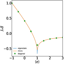
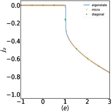
Figure 2: (Color online) Energy dependence of ensemble expectations values of $J_{x}$ and $J_{z}$: The orange line is for the Micro-canonical, while the green dots are for the diagonal ensembles with initial phase $\phi^{\prime}=0$ and increasing $\left<J_{z}\right>/J=z^{\prime}(E)$. The energy dependence of the eigenstate expectation values is also shown. These calculations where performed for $|J|=1000$ and $\Lambda=10$. Notice the strong departure of the diagonal ensemble at $E=1$ from the micro-canonical ensemble.

I Semi-Classical Picture and ETH:

We first consider the case when the assumptions of ETH are valid and the large spin thermalizes. To do so it will be useful to first consider why assumptions of ETH generally imply thermalization. First consider the eigenstate decomposition of the initial state density matrix, $\sum_{nm}c_{n}c_{m}\left|n\right>\left<m\right|$. At long times, $t$ and for sufficiently large $T$, we can expect that only the diagonal terms of the density matrix contribute to observablesD’Alessio et al. (2016); Khripkov et al. (2013):

$$O(t,T)\approx\sum_{m}\left|c_{m}\right|^{2}\left<m\right|O\left|m\right>.$$ (3)

If A3) of ETH is true, then $\left|c_{m}\right|^{2}$ is non zero only in a small energy window. Furthermore, if A1) of ETH holds, then $\left<m\right|O\left|m\right>$ is approximately constant over the eigenstates with significant probability $\left|c_{m}\right|^{2}$. Finally A2) ensures there are multiple eigenstates in the micro-canonical ensemble which can be sampled, and we can conclude that a representative eigenstate $\left<n\right|O\left|n\right>$ can be chosen to factor out of the average in Eq. 3 yielding: $O(t,T)\approx\left<n\right|O\left|n\right>$.

We now use a semi-classical analysis to determine when these three assumptions of ETH hold for the nonlinear spin Hamiltonian. The semi-classical analysis is based on a Wigner-function formalism in which states and operators are represented as functions, $W(z,\phi)$ and $O(z,\phi)$, of $z$, the eigenvalue of $J_{z}/\left|J\right|$, and its conjugate momentum $\phi$. In this formalism, the observables $J_{z}$ and $J_{x}$ are given by $|J|z$ and $|J|\sqrt{1-z^{2}}\cos(\phi)$ respectively, and the Hamiltonian is written asRaghavan et al. (1999):

$$\frac{H(z,\phi)}{|J|}=\frac{\Lambda}{2}z^{2}-\sqrt{1-z^{2}}\cos(\phi)$$ (4)

The expectation values of a state $W(z,\phi)$ with an observable $O(z,\phi)$ is computed with:

$$\left<\psi\right|O\left|\psi\right>=\frac{1}{4\pi}\int_{-1}^{1}\int_{-\pi}^{\pi}dzd\phi W(z,\phi)O(z,\phi).$$ (5)

We use the set of spin coherent states as our initial states because they are regularly created in experimentsZibold et al. (2010); Strobel et al. (2014). In the Wigner-function formalism these states are represented by Gaussian distributions that become more localized around a mean $z^{\prime}$ and a mean $\phi^{\prime}$ as the size of the spin, $|J|$, is increased . Since a state which is more local around a specific $z^{\prime}$ and $\phi^{\prime}$ has smaller energy uncertainty, assumption A3) of ETH is satisfied when $|J|$ is sufficiently large.

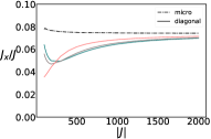
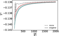
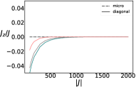
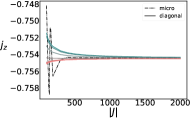
Figure 3: (color online) Thermalization for Self-Trapping and Free-Oscillating Dynamics: In this plot, we show the micro-canonical and diagonal ensemble expectation values as a function of $|J|$ and $\phi^{\prime}$ for $E=0.5$(1st column) and $E=3$ (second column). The color indicates the initial phase $\phi^{\prime}$ where it ranges from 0(dark blue) to $\pi$ (bright pink). When $|J|$ increases, the energy level spacing decreases and the assumptions A2) and A3) of ETH become more valid. Thus for large $|J|$ ETH for the diagonal matrix elements is valid and the dependence of the LTOs on the initial phase is lost. These calculations where done with $\Lambda=10$

We now consider when assumptions A1) and A2) hold by constructing the Wigner functions of the eigenstates via a semi-classical analysis. The zeroth order classical analysis treats Eq. 4 as a classical Hamiltonian which yields the periodic trajectories depicted in Fig. 1. Fig. 1 shows two distinct types of periodic trajectories depending on the energy: for $E<1$, the trajectories known as Josephson oscillationRaghavan et al. (1999) occur in which $z$ and $\phi$ periodically oscillates around a stable fixed point at $(z,\phi)=(0,0)$, while for $E>1$ trajectories called self trappingAlbiez et al. (2005) occur in which $z$ does not change sign, and $\phi$ monotonically increases ($z<0$) or decreases ($z>0$) depending on the sign of $z$. At $E=1$, there is a separatrix separating the two dynamical behaviors.

Using the correspondence between classical periodic trajectories and eigenstatesSakurai (1994), the eigenstate Wigner-functions (EWF) with energy $E$ can be written as $\rho_{E}(z,\phi)=w(E)\delta\boldsymbol{(}H(z,\phi)-E\left|J\right|\boldsymbol{)}$, where $w(E)$ is the normalization of the eigenstate with energy $E$. The quantized energy levels, $E=E_{n}$, are then determined by the ruleChuchem et al. (2010) stating that the area swept out by the eigenstate trajectories is quantized to $2\pi/\left|J\right|$. Thus, the energy difference between the eigenstate trajectories goes to $0$ as $|J|$ is increased, and assumption A2) of ETH holds true.

Considering assumption A1), we first identify that the Hamiltonian in Eq. 4 has two distinct types of eigenstates corresponding to the Josephson oscillation and the self trapping trajectories. The self trapping eigenstates are further structured because, for a given energy $E>1$, there are two disconnected trajectories depending on the initial sign of $z$. These two trajectories will be identified with the sign of $z$ and their associated EWFs are calculated by selecting the correct trajectory when inverting $H(z,\phi)$:

$$\rho_{E\pm}(z,\phi)=w(E)\left|\frac{dH(z,\phi)}{dz}\right|^{-1}\delta\boldsymbol{(}z\pm\left|H^{-1}(E,\phi)\right|\boldsymbol{)}$$ (6)

At lowest order in a semi-classical expansion, these two trajectories correspond to two degenerate eigenstates, while at higher order the degeneracy is liftedPudlik et al. (2014) with splitting exponentially decreasing with $\left|J\right|$. Since this splitting is exponentially small, we will ignore it and assume all measurements occur before its dynamics are realized( $t<T_{t}\approx e^{|J|}$).

For $E\neq 1$, the eigenstate observables will be smooth in energy because, the difference between two neighboring eigenstate trajectories decreases to $0$ as $|J|$ is increased. While for $E=1$, the self trapping trajectories meet the free oscillating ones, a discontinuity emerges, and non analytic behavior of the eigenstate observables is expected. The behavior of the eigenstate observables has been identified previouslyRaghavan et al. (1999); Benitez et al. (2009) and we confirm for $J_{x}$ and $J_{z}$ in Fig. 2.

Thus, we find that away from $E=1$ and for large enough $\left|J\right|$, the assumptions of ETH hold, and we expect the LTOs to be described by a micro-canonical ensemble. While for eigenstates with energy $E\approx 1$, assumption A1) of ETH does not hold, and additional consideration is required to understand the long time behavior.

II Numerical Analysis of the Diagonal Ensemble:

From the analysis of the previous section we expect initial coherent states with $z^{\prime}$ and $\phi^{\prime}$ away from the separatrix to show thermal behavior at long times. Using exact diagonalization, we confirm that memory of the initial state is lost for $E\neq 1$. This is shown in Fig. 3, which demonstrates that the diagonal ensemble for states with different $\phi^{\prime}$, but same $E$, all reproduce the same LTO. We also confirm that a micro-canonical ensemble, and a characteristic eigenstate, describe the LTOs. This is shown in Fig. 2 for $J_{x}$ and $J_{z}$.

Since the hamiltonian is integrable, the off diagonal matrix elements are not random as proposed by ETH, and one can not use ETH to argue that the LTO relax to the time averages predicted by the Diagonal ensemble. Instead, we must check by exact numerical simulation. Doing so for $J_{x}$, we find that the self trapping dynamics and free-oscillating dynamics do in fact relax to a constant value independent of the initial phase $\phi^{\prime}$. This is shown in Fig. 4.

Close to $E=1$, the micro-canonical ensemble and the characteristic eigenstate no longer match LTOs. Failure of the initial states at $E=1$ to thermalize is further demonstrated in Fig. 5, which shows a dramatic dependence of the LTOs on the initial phase, $\phi^{\prime}$. This does not invalidate ETH because assumption A1) of ETH does not hold for these eigenstates.

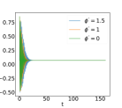
Figure 4: (Color Online) Dynamics of $J_{x}/|J|$ for different values of $\phi^{\prime}$ at energies $E=3$(top), $E=0.5$ (bottom).

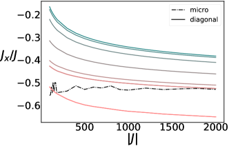
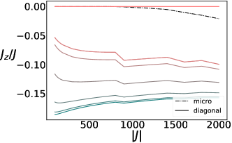
Figure 5: (color online) Failure of Thermalization on the Separatrix: The contents of these plots are equivalent to those in Fig. 3, except they are calculated for initial states with $E=1$. This time, despite the assumptions A2) and A3) becoming more valid as $|J|$ is increased, the assumption A1) remains invalid and the memory of initial phase $\phi^{\prime}$ remains at large $|J|$.

III Semi-Classical Analysis of the Breakdown of Thermalization:

To better understand this breakdown of thermalization we investigate, using the semi-classical analysis, how the $E\approx 1$ eigenstates affect the LTO of the initial coherent states with $E\approx 1$ . We begin by calculating the diagonal ensemble and its expectation values for the initial coherent states used above. Semi-classicallyChuchem et al. (2010) the diagonal ensemble is given as:

$$\rho_{diag}=\frac{1}{4\pi}\int_{-1}^{1}\int_{-\pi}^{\pi}dzd\phi W_{c}(z,\phi,z^{\prime},\phi^{\prime})\rho_{E,s}(z,\phi)$$ (7)

where $W_{c}$ is the initial coherent state Gaussian distribution centered around $z^{\prime}$ and $\phi^{\prime}$ with variance $\sim\frac{1}{J}$, and the EWF, $\rho_{E,\pm}$, is given by the delta function in Eq. 6.

To calculate the LTOs, one must convolve the diagonal ensemble with the eigenstate expectation values:

$$O_{diag}(\phi^{\prime},z^{\prime})=\int_{-1}^{\Lambda/2}dE\sum_{s}\rho_{diag}(\phi^{\prime},z^{\prime},E,s)O(E,s)$$ (8)

where the sum over $s$ is the sum over self trapping states when $E>1$ and a fixed $s=0$ for $E<1$, and $O(E,s)$ is the eigenstate expectation value calculated using Eq. 5 with $W(z,\phi)=\rho_{E,s}(z,\phi)$.

Understanding this integral, and consequently why the LTOs encode information about the initial phase $\phi^{\prime}$, requires understanding the structure of the eigenstates and their EWFs. While an EWF is constrained to an equal energy surface, the shape of the energy surface affects how the EWF is distributed within the energy surface. This is captured by the Jacobian, $\left|\frac{dH(z,\phi)}{dz}\right|$, which appears in Eq. 6 due to the transformation of the energy delta function to phase space coordinates. Take the $s=1$ self trapping eigenstate for example. If one integrates out $z$ using the delta function, the Jacobian $|\frac{dH}{dz}|(E,\phi)=|\frac{d\phi}{dt}|(E,\phi)$ weighs the EWF. Therefore, the EWF will have more weight in regions where $\phi$ is changing slower in time.

On the separatrix, $E=1$, the classical spin comes to a complete stop on the unstable fixed point; the Jacobian limits to $0$, $\text{lim}_{E\rightarrow 1}\text{lim}_{\phi\rightarrow\pi}|\frac{dH}{dz}|(E,\phi)=0$; and the EWFs with $E\rightarrow 1$ become localized on the unstable fixed point:$\rho_{E\rightarrow 1}(z,\phi)\approx\delta(z)\delta(\phi-\pi)$. The singularity of this localization result in the non-analytic behavior of the eigenstate expectation values near $E=1$ (see for example $J_{x}$ in Fig. 2).

This singular localization also produces a non-analyticity in the eigenstate overlaps for the set of initial coherent states with $E\approx 1$, but $\phi^{\prime}\neq\pi$. Since these initial states have Wigner functions localized around $\phi^{\prime}$ and $z^{\prime}=H^{-1}(E=1,\phi^{\prime})$ and the EWFs for $E\approx 1$ are localized around $\phi=\pi\neq\phi^{\prime}$ and $z=0\neq z^{\prime}$, their overlap integrals in Eq. 8 will vanish.

These two non-analyticities are integrated over in Eq. 8 and results in the memory effects depicted in Fig. 5. In one limit, an initial coherent state with $\phi^{\prime}\approx\pi$ will overlap the unstable fixed point eigenstate at $E=1$, and the LTOs will closely match the observables of that same eigenstate($J_{z}=0$ and $J_{x}=-1$). In the other limit, when the initial $\phi^{\prime}$ is away from $\pi$, the initial coherent state will have negligible overlap with the $E=1$ eigenstate, the LTOs will depart from the observables of the $E=1$ eigenstate. This is depicted in Fig. 5, in which the closer $\phi^{\prime}$ is to $\pi$, the closer $j_{z}=J_{z}/J$ and $j_{x}=J_{x}/J$ approach $0$ and $-1$ respectively.

Figure 6: (Color Online) Classical fit to exact numerical calculations of diagonal ensemble. This plot shows the $\sqrt{\left|J\right|ln\left|J\right|}$ scaling of $j_{x}=J_{x}/J$ for the diagonal ensemble of a set of initial states with energy $E=1$ and different $\phi^{\prime}$ and $\left|J\right|$. The dots are computed using exact diagonalization and the color indicates the initial $\phi^{\prime}$ as in Fig. 3. Eq. 11 predicts $\sqrt{\left|J\right|ln\left|J\right|}$ and the linear dashed lines are given by Eq. 11 with $F(\phi^{\prime})$ fit to match the exact calculations for $|J|>500$.

IV Large $|J|$ behaviour of Initial State Memory

To capture this behavior analytically, we perform a saddle point expansion for the integral Eq. 8. A similar saddle point approximation was done in Mathew and Tiesinga (2017); Chuchem et al. (2010), but only for an initial state on the unstable fixed point. To capture how the long time memory depends on the size of the spin $\left|J\right|$, we perform the saddle point for initial states computed off the unstable fixed point. The results in Mathew and Tiesinga (2017); Chuchem et al. (2010) will not work here because the diagonal ensemble has a qualitatively different saddle point structure for states on and off the unstable fixed pointsChuchem et al. (2010).

To perform the saddle point approximation away from the unstable fixed point, we begin with finding the diagonal ensemble $\rho_{diag}(\phi^{\prime},z^{\prime},E,z)$ by evaluating the integral in Eq. 7. For large $|J|$, the integral is restricted over a region in the vicinity of $z^{\prime}$ and $\phi^{\prime}$. Since this region is away from the unstable fixed point, the equal energy countor can be approximated as a line and the Jacobian $\left|\frac{dH(z,\phi)}{dz}\right|^{-1}$ is approximately constant. Performing the Dirac delta and Gaussian integrations yields:

$$\rho_{diag} (\phi^{\prime},z^{\prime},E,s)\sim e^{-\frac{(E-H(\phi^{\prime},z^{\prime}))^{2}}{2\sigma^{2}(\phi^{\prime},z^{\prime})}+\text{ln}(w(E))}$$ (9)

where $w(E)$ is the eigenstate normalization. The Gaussian variance $\sigma(\phi^{\prime},z^{\prime})$ is given in Appendix B, and scales with $\left|J\right|$ as $\sim\frac{1}{\sqrt{\left|J\right|}}$ with proportionality dependent on $\phi^{\prime}$ and $z^{\prime}$.

For initial states away from the separatrix, $w(E)$ is approximately constantChuchem et al. (2010), and the diagonal ensemble is a gaussian. This is not the case for initial states on the separatrix. Instead, the asymptotically slow dynamics, and consequently the asymptotic divergence of the Jacobian, near the unstable fixed point, forces an asymptotic vanishing of $w(E)$, and consequently $\rho_{diag}(\phi^{\prime},z^{\prime},E,s)$, at $E=1$. Computing $w(E)$ in Appendix A, we find that it vanishes as $\sim 1/Ln(|1-E|)$, where the proportionality is different depending on if $E$ is greater or less then $1$.

Since, $\rho_{diag}(\phi^{\prime},z^{\prime},E,s)$ is $0$ at $E=1$ and in the limit $E\rightarrow\pm\infty$, it possesses a double peak structure in $E$. This is qualitatively different from the single peak saddle point structure used to perform the calculations in Mathew and Tiesinga (2017); Chuchem et al. (2010). The locations of these two peaks determines our saddles and are computed in Appendix C. In the large $|J|$ limit, these saddles become symmetric about $E=1$ given by $E_{s}=1\pm\delta$, and go to $E=1$ as $\delta\sim\frac{1}{2JLn(J)}$.

We then evaluate the integral in Eq. 8 at these saddles:

$$O_{diag}(z^{\prime},\phi^{\prime})=\int\rho_{diag}(E,z^{\prime},\phi^{\prime})O(E)\approx$$ (10)

$$\frac{1}{3}\left[2O(1+|\delta|)+O(1-|\delta|)\right]$$

where the factor of $2$ for $+|\delta|$ occurs because $\rho_{diag}(E,z^{\prime},\phi^{\prime})$ in the $\delta\rightarrow+0$ limit is twice as large as in the $\delta\rightarrow-0$ limit(See $w(E)$ in Appendix A). In Appendix D we compute $J_{x}(1\pm|\delta|)$ and $J_{z}(1\pm|\delta|)$ for small $\delta$ using methods similar to Mathew and Tiesinga (2017); Chuchem et al. (2010). Using these results, we get:

$$j_{z,diag}(\left|J\right|,E=1,\phi^{\prime}) = \frac{4\pi\sqrt{(\Lambda-1})}{3\Lambda ln\left[F(\phi^{\prime})\left|J\right|ln[\left|J\right|]\right]}$$ (11)

$$j_{x,diag}(\left|J\right|,E=1,\phi^{\prime}) = -1+\frac{1}{\sqrt{F(\phi^{\prime})\left|J\right|ln[\left|J\right|]}}\frac{3+\Lambda}{3(\Lambda-1)}$$

where the factor $F(\phi^{\prime})=\left[2\sigma(z^{\prime},\phi^{\prime})^{2}\left|J\right|\right]^{-1}$, $j_{x(z)}=J_{x(z)}/J$, and $z^{\prime}$ is fixed by energy $z^{\prime}=H^{-1}(E=1,\phi^{\prime})$. The factor $F(\phi^{\prime})$ is constant in $\left|J\right|$ but has a non-trivial dependence on the initial phase $\phi^{\prime}$ via $\sigma(z^{\prime},\phi^{\prime})$, the energy variance of the coherent state. This non-trivial dependence in $\phi^{\prime}$ describes the memory effects shown in Fig. 5 for the initial states with $\phi^{\prime}\neq\pi$. For the initial states with $\phi^{\prime}\approx\pi$ we must use the single peak saddle point approximation outlined by Chuchem et al. (2010); Mathew and Tiesinga (2017) which give a different scaling to the fixed point values of $J_{x}\rightarrow-1$ and $J_{z}=0$.

While the exact diagonal ensemble for $J_{z}$ becomes numerically unstable for large $|J|$, we can still compare exact results for $J_{x}$ with Eq. 11. This comparison is shown in Fig. 6, where the $\sqrt{\left|J\right|ln[\left|J\right|]}$ scaling is confirmed.

V Discussion and Possible Experimental Realizations:

Above we discussed how, for the large non-linear spin with energy $E\neq 1$, the assumptions of ETH hold and the spin thermalizes, while for $E=1$ the spin does not thermalize. This lack of thermalization is particularly interesting because the remembered quantity, $\phi$, is not a conserved quantity of the integrable classical dynamics. It is therefore a novel form of quantum memory, which is lost in the classical limit $J\rightarrow\infty$ (See Eq. 11).

Our results are particularly important in the context of recent works on out-of-time order correlations (OTOCs)Pilatowsky-Cameo et al. (2020); Xu et al. (2020); Rozenbaum et al. (2020). Recently OTOCs have become a diagnostic of quantum many body chaos, and have been shown to display exponentially fast growth when the dynamics of an effective classical system displays chaosLashkari et al. (2013); Maldacena et al. (2016); Roberts et al. (2015); Shenker and Stanford (2014a, b, 2015). In the works Pilatowsky-Cameo et al. (2020); Xu et al. (2020); Rozenbaum et al. (2020), they found that classically unstable fixed points can produce exponentially growing OTOCs in systems with an integrable classical counterpart, and suggest exponential growth of OTOCs is not a predictor of quantum chaosXu et al. (2020). Our results further support this conclusion, showing that despite the chaotic like behavior suggested by OTOCs, dynamics near the unstable fixed point are precisely those which depict long time memory of an initial state.

The appearance of unstable fixed points in semi-classical dynamics is ubiquitous, and we expect this mechanism for the breakdown of thermalization to be general. While here we discussed a classically two-dimensional, integrable system, the Berry ConjectureBerry (1977); D’Alessio et al. (2016) suggests that the correspondence of eigenstates to trajectories, generalizes to a correspondence to micro-canonical ensembles in higher dimensional chaotic systems. Since the micro-canonical ensemble is also described by a delta function in energy, the Jacobian produced when transforming to the phase space coordinates would again reveal localization due to slow classical dynamics. One might again expect singularities due to a localized eigenstate and for them to produce memory effects following similar arguments as discussed above. This time, rather than the phase along a separatrix, it would be the distance to the unstable fixed point on the energy surface that is remembered. This is an exciting possibility which requires further investigation.

This mechanism for the breakdown of thermalization may be observable in ultra cold BECsZibold et al. (2010); Muessel et al. (2015, 2015) in which the bosons can be condensed into one of two modes such as two different hyperfine states. A spin boson mapping then yields the non-linear spin Hamiltonian, where the parameter $\Lambda$ is a ratio between the bosonic interaction energy and the energy associated with the tunneling between the two modes. Previous work has suggested that the other bosonic modes do not affect the dynamics on experimental time scalesLovas et al. (2017); Khripkov et al. (2013). Future work may find it interesting to investigate the effect of additional modes and may find connection with other forms of novel long time dynamicsLerose et al. (2018).

Appendix A Eigenstate normalization: $\omega(E)$

. In the main text we defined the semi-classical eigenstate Wigner function (EWF) as:

$$\rho_{E}(z,\phi)=\omega(E)\delta(H(z,\phi)-E)$$ (12)

where the Hamiltonian is given as:

$$H=\frac{\Lambda z^{2}}{2}-\sqrt{1-z^{2}}\cos(\phi),$$ (13)

and the normalization $\omega(E)$ is given as:

$$\omega(E)^{-1}=\int\int dzd\phi\delta(E-H(z,\phi)).$$ (14)

To compute this integral, we focus on the energy close to the separatrix, $E=1\pm\left|\delta\right|$, and expand the Hamiltonian around $E=1$:

$$H-1=\frac{\Lambda-1}{2}z^{2}-\frac{(\phi-\pi)^{2}}{2}$$ (15)

Close to the unstable fixed point the trajectories trace out a hyperbola:

$$z = \pm\sqrt{\frac{2}{\Lambda-1}}\sqrt{\frac{\phi^{2}}{2}+(E-1)}$$ (16)

$$\phi = \sqrt{2(1-E)+(\Lambda-1)z^{2}}$$

The Jacobian for both these trajectories are:

$$\left|\frac{dH}{dz}\right| =(\Lambda-1)z= \sqrt{(\Lambda-1)}\sqrt{2(E-1)+\phi^{2}}$$ (17)

$$\left|\frac{dH}{d\phi}\right| =\phi= \sqrt{(\Lambda-1)}\sqrt{\frac{2(1-E)}{(\Lambda-1)}+z^{2}}.$$

Since the inverse Jacobians, $\left|\frac{dH}{d\phi}\right|^{-1}$ and $\left|\frac{dH}{dz}\right|^{-1}$, contribute the most near the unstable fixed point and we can expand the integrand for $\omega(E)^{-1}$ near them and write:

$$\omega(1+|\delta|)^{-1} =\int_{-r_{+}}^{r_{+}}\left|\frac{dH}{dz}\right|^{-1}(\phi,\delta)+C_{+}$$ (18)

$$\omega(1-|\delta|)^{-1} =\int_{-r_{-}}^{r_{-}}\left|\frac{dH}{d\phi}\right|^{-1}(z,\delta)+C_{-}$$

where $r_{\pm}$ denotes the limits where the hyperbolic expansion is valid and $C_{\pm}$ are small and approximately constant for $\delta$ small. Defining $a$ as:

$$a_{+}=2(E-1)$$ (19)

$$a_{-}=\frac{2(1-E)}{\Lambda-1},$$

these integrals can be expressed as:

$$\frac{1}{\sqrt{a(\Lambda-1})}\int_{-r}^{r}\frac{1}{\sqrt{1-a^{-1}x^{2}}}dx=$$ (20)

$$\frac{1}{\sqrt{(\Lambda-1})}\left[\sinh^{-1}\left(\frac{r}{\sqrt{a}}\right)\right]$$

and for $E\approx 1$, this approximates to as:

$$\omega(1+|\delta|)^{-1}=-\frac{Ln\left(|\delta|\right)}{2\sqrt{(\Lambda-1})}$$ (21)

$$\omega(1-|\delta|)^{-1}=-\frac{Ln\left(|\delta|\right)}{\sqrt{(\Lambda-1})}$$

Appendix B Energy Uncertainty of Diagonal Ensemble for a Coherent State: $\sigma$

To approximate the eigenstate overlap for initial states on the separatrix but away from the fixed points, we expand the energy to linear order in $z$ and $\phi$:

$$H=\kappa_{1}\phi+\gamma_{1}z+E_{0}$$ (22)

We first write the coherent state with initial imbalance $z^{\prime}$ and phase $\phi^{\prime}$ as:

$$\rho(N,z^{\prime},\phi^{\prime},z,\phi)=$$ (23)

$$\frac{\alpha_{z}(N,z^{\prime})\alpha_{\phi}(N,z^{\prime})}{\pi}e^{-\alpha_{z}(N,z^{\prime})(z-z^{\prime})^{2}-\alpha_{\phi}(N,z^{\prime})(\phi-\phi^{\prime})^{2}}$$

where the inverse variances are:

$$\alpha_{\phi}(J,z^{\prime}) = \frac{1}{2}J\left(1-z^{2}\right)$$ (24)

$$\alpha_{z}(J,z^{\prime}) = \frac{2J}{1-z^{2}}$$

The eigenstate overlap is then given as:

$$\rho_{diag}(z^{\prime},\phi^{\prime},E,s)=$$ (25)

$$\frac{\omega(E)}{\gamma_{1}}\int\text{d$\phi\rho$}\left(N,z^{\prime},\phi^{\prime},\frac{\delta_{0}-\kappa_{1}\phi}{\gamma},\phi\right),$$

where $\delta_{0}=E-E_{0}$, and integrates to give:

$$\frac{\omega(E)}{\gamma_{1}}\frac{\sqrt{\alpha_{z}(N,z^{\prime})\alpha_{\phi}(N,z^{\prime})}}{\sqrt{\pi}\sqrt{\alpha_{\phi}+\frac{\kappa_{1}^{2}\alpha_{z}}{\gamma_{1}^{2}}}}\exp\left(-\frac{\delta_{0}^{2}\alpha_{\phi}\alpha_{z}}{\gamma_{1}^{2}\alpha_{\phi}+\kappa_{1}^{2}\alpha_{z}}\right)$$ (26)

Where the energy uncertainty $\sigma$ is given by:

$$\sigma(\phi^{\prime},z^{\prime})=-\frac{\gamma_{1}^{2}\alpha_{\phi}+\kappa_{1}^{2}\alpha_{z}}{2\alpha_{\phi}\alpha_{z}}$$ (27)

depends on the coherent state via the uncertainties $\alpha_{z}$ and $\alpha_{\phi}$.

Appendix C Double Peak Saddles

Analytic solutions for the saddle point only exist if $E_{0}=1$ so we focus on coherent states on this line. To find the saddle points we rewrite $\rho_{diag}$ as:

$$\rho_{diag}(E=1\pm\left|\delta\right|)=\frac{K_{\pm}}{(1-G_{\pm}Ln[\delta])}Exp[-2JF\delta^{2}]$$ (28)

where $K_{\pm}$ and $G_{\pm}$ are constants in $\delta$, depend on $C_{\pm}$, and with $\pm$ depending on the sign of $\delta$ . This function has a saddle at:

$$|\delta|=\frac{i}{\sqrt{(2JF)W_{-1}(-\frac{e^{-2/G_{\pm}}}{F2J})}}$$ (29)

Where the product log, $W_{-1}(X)$, is the inverse of $e^{x}x$: $W_{-1}(e^{x}x)=x$ and the _-1 says to take the negative branch. For small $x$ we get:

$$\lim_{x\rightarrow 0^{-}}\frac{W_{-1}(x)}{Ln(x)}=1$$ (30)

and we know $W_{-1}(x)\approx Ln(-x)-Ln(-Ln(-x))+\dots$ We therefore get the approximation:

$$|\delta|\approx\frac{i}{\sqrt{2JFLn(\frac{e^{-2/G_{\pm}}}{F2J})}}$$ (31)

Which in the large-$J$ limit goes as:

$$\frac{1}{\sqrt{2JFLn(J)}}$$ (32)

and

$$2JF=\frac{\alpha_{\phi}\alpha_{z}}{\gamma_{1}^{2}\alpha_{\phi}+\kappa_{1}^{2}\alpha_{z}}$$ (33)

Thus the difference in initial states on the separatrix again shows up in the scaling to the large $J$ limit. Also note $G$ comes from $\omega(E)$ which depends on which side of the separatrix we are on (sign of $\delta$). In the large-$J$ limit the points become symmetric as indicated by the lack of dependence on $G$.

Appendix D Eigenstate observables close to the separatrix

Next we compute the eigenstate observables, $O(E)$, which are given as

$$\omega(E)\int O(z,\phi)\delta[H(z,\phi)-E].$$ (34)

$J_{z}$ for $\Lambda$ large has a amazingly simple solution. For $E<1$, $J_{z}(E)=0$ for $E>1$ we integrate:

$$\int dz\delta[H(z,\phi)-E]=\int_{-\pi}^{\pi}d\phi z(\phi)\left|\frac{dH}{dz}\right|^{-1}$$ (35)

and for $\Lambda>>1$, $\left|\frac{dH}{dz}\right|^{-1}\approx\Lambda z$, the $z$’s cancel and we get

$$J_{z}(E)=\frac{\omega(E)2\pi}{\Lambda}.$$ (36)

$J_{x}$ is more involved. We will take the same approach as the integral for $\omega(E)$. We assume the integral is dominated by the contribution near the unstable fixed point. Doing so allows us to expand $J_{x}$ near the unstable fixed point: $J_{x}\approx-1+\phi^{2}/2$. Solving for $\phi$, we find that it is written as: $J_{x}\approx\frac{\Lambda-1}{2}z^{2}-E$.

$$J_{x}(1+|\delta|)^{-1}=$$ (37)

$$\omega(E)(\Lambda-1)\int_{-r_{+}}^{r_{+}}\left(-\frac{E}{\Lambda-1}+z^{2}/2\right)\left|\frac{dH}{dz}\right|^{-1}(\phi,\delta)+K_{+}$$

$$J_{x}(1-|\delta|)^{-1}=$$

$$\omega(E)\int_{-r_{-}}^{r_{-}}(-1+\phi^{2}/2)\left|\frac{dH}{d\phi}\right|^{-1}(z,\delta)+K_{-}$$

Similar to the integral for $\omega(E)$, these can be computed and in the limit of small $\delta$ we get:

$$J_{x}(1+|\delta|)^{-1} = -1+\omega(\left|\delta\right|)\left(K_{+}-\frac{\left|\delta\right|Ln(\left|\delta\right|)}{(\Lambda-1)^{3/2}}\right)$$ (38)

$$J_{x}(1-|\delta|)^{-1} = -1+\omega(\left|\delta\right|)\left(K_{-}-\frac{\left|\delta\right|Ln(\left|\delta\right|)}{\sqrt{\Lambda-1}}\right)$$

$\omega(\left|\delta\right|)$ goes to $0$ faster than $\omega(\left|\delta\right|)\left|\delta\right|Ln(\left|\delta\right|)$ and we get:

$$J_{x}(1+|\delta|)^{-1} = -1-\omega(\left|\delta\right|)\frac{\left|\delta\right|Ln(\left|\delta\right|)}{(\Lambda-1)^{3/2}}$$ (39)

$$J_{x}(1-|\delta|)^{-1} = -1-\omega(\left|\delta\right|)\frac{\left|\delta\right|Ln(\left|\delta\right|)}{\sqrt{\Lambda-1}}$$

Substituting $\omega$:

$$J_{x}(1+|\delta|)^{-1} = -1+\frac{2\left|\delta\right|}{\Lambda-1}$$ (40)

$$J_{x}(1-|\delta|)^{-1} = -1+\left|\delta\right|$$

$$J_{z}(1+|\delta|) = \frac{4\pi\sqrt{(\Lambda-1})}{\Lambda Ln\left(|\delta|\right)}$$

$$J_{z}(1-|\delta|) = 0$$

References

- Bloch et al. (2008) Immanuel Bloch, Jean Dalibard, and Wilhelm Zwerger, “Many-body physics with ultracold gases,” Rev. Mod. Phys. 80, 885–964 (2008).
- Ludlow et al. (2015) Andrew D. Ludlow, Martin M. Boyd, Jun Ye, E. Peik, and P. O. Schmidt, “Optical atomic clocks,” Rev. Mod. Phys. 87, 637–701 (2015).
- Shaffer et al. (2018) J. P. Shaffer, S. T. Rittenhouse, and H. R. Sadeghpour, “Ultracold Rydberg molecules,” Nature Communications 9, 1965 (2018).
- Zibold et al. (2010) Tilman Zibold, Eike Nicklas, Christian Gross, and Markus K. Oberthaler, “Classical Bifurcation at the Transition from Rabi to Josephson Dynamics,” Physical Review Letters 105, 204101 (2010).
- Deutsch (1991) J. M. Deutsch, “Quantum statistical mechanics in a closed system,” Phys. Rev. A 43, 2046–2049 (1991).
- Srednicki (1994) Mark Srednicki, “Chaos and quantum thermalization,” Phys. Rev. E 50, 888–901 (1994).
- Rigol et al. (2008) Marcos Rigol, Vanja Dunjko, and Maxim Olshanii, “Thermalization and its mechanism for generic isolated quantum systems,” Nature 452, 854–858 (2008).
- D’Alessio et al. (2016) Luca D’Alessio, Yariv Kafri, Anatoli Polkovnikov, and Marcos Rigol, “From quantum chaos and eigenstate thermalization to statistical mechanics and thermodynamics,” Advances in Physics 65, 239–362 (2016).
- Deutsch (2018) Joshua M. Deutsch, “Eigenstate Thermalization Hypothesis,” Rep. Prog. Phys. 81, 082001 (2018).
- Jensen and Shankar (1985) R. V. Jensen and R. Shankar, “Statistical Behavior in Deterministic Quantum Systems with Few Degrees of Freedom,” Phys. Rev. Lett. 54, 1879–1882 (1985).
- Mori et al. (2018) Takashi Mori, Tatsuhiko N Ikeda, Eriko Kaminishi, and Masahito Ueda, “Thermalization and prethermalization in isolated quantum systems: a theoretical overview,” Journal of Physics B: Atomic, Molecular and Optical Physics 51, 112001 (2018).
- Polkovnikov et al. (2011) Anatoli Polkovnikov, Krishnendu Sengupta, Alessandro Silva, and Mukund Vengalattore, “Colloquium: Nonequilibrium dynamics of closed interacting quantum systems,” Rev. Mod. Phys. 83, 863–883 (2011).
- Batchelor and Foerster (2016) Murray T. Batchelor and Angela Foerster, “Yang–Baxter integrable models in experiments: From condensed matter to ultracold atoms,” J. Phys. A: Math. Theor. 49, 173001 (2016).
- Cassidy et al. (2011) Amy C. Cassidy, Charles W. Clark, and Marcos Rigol, “Generalized Thermalization in an Integrable Lattice System,” Phys. Rev. Lett. 106, 140405 (2011).
- Imbrie et al. (2017) John Z. Imbrie, Valentina Ros, and Antonello Scardicchio, “Local integrals of motion in many-body localized systems,” Annalen der Physik 529, 1600278 (2017).
- Nandkishore and Huse (2015) Rahul Nandkishore and David A. Huse, “Many-Body Localization and Thermalization in Quantum Statistical Mechanics,” Annual Review of Condensed Matter Physics 6, 15–38 (2015).
- Abanin et al. (2019) Dmitry A. Abanin, Ehud Altman, Immanuel Bloch, and Maksym Serbyn, “Colloquium: Many-body localization, thermalization, and entanglement,” Rev. Mod. Phys. 91, 021001 (2019).
- Tikhonenkov et al. (2013) Igor Tikhonenkov, Amichay Vardi, James R. Anglin, and Doron Cohen, “Minimal Fokker-Planck Theory for the Thermalization of Mesoscopic Subsystems,” Phys. Rev. Lett. 110, 050401 (2013).
- Arwas et al. (2015) Geva Arwas, Amichay Vardi, and Doron Cohen, “Superfluidity and Chaos in low dimensional circuits,” Scientific Reports 5, 13433 (2015).
- Khripkov et al. (2016) Christine Khripkov, Doron Cohen, and Amichay Vardi, “Thermalization of Bipartite Bose–Hubbard Models,” J. Phys. Chem. A 120, 3136–3141 (2016).
- Khripkov et al. (2018) Christine Khripkov, Amichay Vardi, and Doron Cohen, “Semiclassical theory of strong localization for quantum thermalization,” Phys. Rev. E 97, 022127 (2018).
- Arwas and Cohen (2016) Geva Arwas and Doron Cohen, “Chaos and two-level dynamics of the atomtronic quantum interference device,” New J. Phys. 18, 015007 (2016).
- Arwas and Cohen (2017) Geva Arwas and Doron Cohen, “Chaos, metastability and ergodicity in Bose-Hubbard superfluid circuits,” AIP Conference Proceedings 1912, 020001 (2017).
- Arwas and Cohen (2019) Geva Arwas and Doron Cohen, “Monodromy and chaos for condensed bosons in optical lattices,” Phys. Rev. A 99, 023625 (2019).
- Pizzi et al. (2019a) Andrea Pizzi, Fabrizio Dolcini, and Karyn Le Hur, “Quench-induced dynamical phase transitions and -synchronization in the bose-hubbard model,” Phys. Rev. B 99, 094301 (2019a).
- Pizzi et al. (2019b) Andrea Pizzi, Johannes Knolle, and Andreas Nunnenkamp, “Period- discrete time crystals and quasicrystals with ultracold bosons,” Phys. Rev. Lett. 123, 150601 (2019b).
- Strobel et al. (2014) Helmut Strobel, Wolfgang Muessel, Daniel Linnemann, Tilman Zibold, David B. Hume, Luca Pezze’, Augusto Smerzi, and Markus K. Oberthaler, “Fisher information and entanglement of non-Gaussian spin states,” Science 345, 424–427 (2014).
- Raghavan et al. (1999) S. Raghavan, A. Smerzi, S. Fantoni, and S. R. Shenoy, “Coherent oscillations between two weakly coupled Bose-Einstein condensates: Josephson effects, pi oscillations, and macroscopic quantum self-trapping,” Physical Review A 59, 620–633 (1999).
- Micheli et al. (2003) A. Micheli, D. Jaksch, J. I. Cirac, and P. Zoller, “Many-particle entanglement in two-component Bose-Einstein condensates,” Physical Review A 67, 013607 (2003).
- Mahmud et al. (2005) Khan W. Mahmud, Heidi Perry, and William P. Reinhardt, “Quantum phase-space picture of Bose-Einstein condensates in a double well,” Physical Review A 71, 023615 (2005).
- Chuchem et al. (2010) Maya Chuchem, Katrina Smith-Mannschott, Moritz Hiller, Tsampikos Kottos, Amichay Vardi, and Doron Cohen, “Quantum dynamics in the bosonic Josephson junction,” Physical Review A 82, 053617 (2010).
- Huang et al. (2012) Yixiao Huang, Wei Zhong, Zhe Sun, and Xiaoguang Wang, “Fisher-information manifestation of dynamical stability and transition to self-trapping for Bose-Einstein condensates,” Physical Review A - Atomic, Molecular, and Optical Physics 86, 1–7 (2012).
- Lapert et al. (2012) M. Lapert, G. Ferrini, and D. Sugny, “Optimal control of quantum superpositions in a bosonic Josephson junction,” Physical Review A - Atomic, Molecular, and Optical Physics 85, 1–13 (2012).
- Khripkov et al. (2013) Christine Khripkov, Doron Cohen, and Amichay Vardi, “Temporal fluctuations in the bosonic Josephson junction as a probe for phase space tomography,” J. Phys. A: Math. Theor. 46, 165304 (2013).
- Lovas et al. (2017) Izabella Lovas, József Fortágh, Eugene Demler, and Gergely Zaránd, “Entanglement and entropy production in coupled single-mode Bose-Einstein condensates,” Phys. Rev. A 96, 023615 (2017).
- Mathew and Tiesinga (2017) R. Mathew and E. Tiesinga, “Phase-space mixing in dynamically unstable, integrable few-mode quantum systems,” Phys. Rev. A 96, 013604 (2017).
- Kelly et al. (2019) Shane P. Kelly, Eddy Timmermans, and S.-W. Tsai, “Detecting macroscopic indefiniteness of cat states in bosonic interferometers,” Phys. Rev. A 100, 032117 (2019).
- Hennig et al. (2012) Holger Hennig, Dirk Witthaut, and David K. Campbell, “Global phase space of coherence and entanglement in a double-well Bose-Einstein condensate,” Phys. Rev. A 86, 051604 (2012).
- Morita et al. (2006) Hiroyuki Morita, Hiromasa Ohnishi, João [da Providência], and Seiya Nishiyama, “Exact solutions for the LMG model Hamiltonian based on the Bethe ansatz,” Nuclear Physics B 737, 337 – 350 (2006).
- Polkovnikov (2010) Anatoli Polkovnikov, “Phase space representation of quantum dynamics,” Annals of Physics 325, 1790 – 1852 (2010).
- Mori (2017) Takashi Mori, “Classical ergodicity and quantum eigenstate thermalization: Analysis in fully connected ising ferromagnets,” Phys. Rev. E 96, 012134 (2017).
- Albiez et al. (2005) Michael Albiez, Rudolf Gati, Jonas Fölling, Stefan Hunsmann, Matteo Cristiani, and Markus K. Oberthaler, “Direct observation of tunneling and nonlinear self-trapping in a single bosonic josephson junction,” Physical Review Letters 95, 010402–010402 (2005).
- Sakurai (1994) J. J. Sakurai, Modern quantum mechanics (Addison-Wesley Pub. Co, Reading, Mass, 1994).
- Pudlik et al. (2014) Tadeusz Pudlik, Holger Hennig, Dirk Witthaut, and David K. Campbell, “Tunneling in the self-trapped regime of a two-well Bose-Einstein condensate,” Phys. Rev. A 90, 053610 (2014).
- Benitez et al. (2009) S. F. Caballero Benitez, V. Romero-Rochin, and R. Paredes, “Delocalization to self-trapping transition of a Bose fluid confined in a double well potential. An analysis via one- and two-body correlation properties,” Journal of Physics B: Atomic, Molecular and Optical Physics 43, 115301–115301 (2009).
- Pilatowsky-Cameo et al. (2020) Saúl Pilatowsky-Cameo, Jorge Chávez-Carlos, Miguel A. Bastarrachea-Magnani, Pavel Stránský, Sergio Lerma-Hernández, Lea F. Santos, and Jorge G. Hirsch, “Positive quantum lyapunov exponents in experimental systems with a regular classical limit,” Phys. Rev. E 101, 010202 (2020).
- Xu et al. (2020) Tianrui Xu, Thomas Scaffidi, and Xiangyu Cao, “Does scrambling equal chaos?” Phys. Rev. Lett. 124, 140602 (2020).
- Rozenbaum et al. (2020) Efim B. Rozenbaum, Leonid A. Bunimovich, and Victor Galitski, “Early-time exponential instabilities in nonchaotic quantum systems,” Phys. Rev. Lett. 125, 014101 (2020).
- Lashkari et al. (2013) Nima Lashkari, Douglas Stanford, Matthew Hastings, Tobias Osborne, and Patrick Hayden, “Towards the fast scrambling conjecture,” J. High Energ. Phys. 2013, 22 (2013).
- Maldacena et al. (2016) Juan Maldacena, Stephen H. Shenker, and Douglas Stanford, “A bound on chaos,” J. High Energ. Phys. 2016, 106 (2016).
- Roberts et al. (2015) Daniel A. Roberts, Douglas Stanford, and Leonard Susskind, “Localized shocks,” J. High Energ. Phys. 2015, 51 (2015).
- Shenker and Stanford (2014a) Stephen H. Shenker and Douglas Stanford, “Black holes and the butterfly effect,” J. High Energ. Phys. 2014, 67 (2014a).
- Shenker and Stanford (2014b) Stephen H. Shenker and Douglas Stanford, “Multiple shocks,” J. High Energ. Phys. 2014, 46 (2014b).
- Shenker and Stanford (2015) Stephen H. Shenker and Douglas Stanford, “Stringy effects in scrambling,” arXiv:1412.6087 [hep-th] (2015), arXiv:1412.6087 [hep-th] .
- Berry (1977) M V Berry, “Regular and irregular semiclassical wavefunctions,” Journal of Physics A: Mathematical and General 10, 2083–2091 (1977).
- Muessel et al. (2015) W. Muessel, H. Strobel, D. Linnemann, T. Zibold, B. Juliá-Díaz, and M. K. Oberthaler, “Twist-and-turn spin squeezing in Bose-Einstein condensates,” Phys. Rev. A 92, 023603 (2015).
- Lerose et al. (2018) Alessio Lerose, Jamir Marino, Bojan Žunkovič, Andrea Gambassi, and Alessandro Silva, “Chaotic Dynamical Ferromagnetic Phase Induced by Nonequilibrium Quantum Fluctuations,” Phys. Rev. Lett. 120, 130603 (2018).