Improvements to Target-Based 3D LiDAR to Camera Calibration

Abstract

The rigid-body transformation between a LiDAR and monocular camera is required for sensor fusion tasks, such as SLAM. While determining such a transformation is not considered glamorous in any sense of the word, it is nonetheless crucial for many modern autonomous systems. Indeed, an error of a few degrees in rotation or a few percent in translation can lead to 20 cm reprojection errors at a distance of 5 m when overlaying a LiDAR image on a camera image. The biggest impediments to determining the transformation accurately are the relative sparsity of LiDAR point clouds and systematic errors in their distance measurements. This paper proposes (1) the use of targets of known dimension and geometry to ameliorate target pose estimation in face of the quantization and systematic errors inherent in a LiDAR image of a target, (2) a fitting method for the LiDAR to monocular camera transformation that avoids the tedious task of target edge extraction from the point cloud, and (3) a “cross-validation study” based on projection of the 3D LiDAR target vertices to the corresponding corners in the camera image. The end result is a 50% reduction in projection error and a 70% reduction in its variance with respect to baseline.

I Introduction and Related Work

The desire to produce 3D-semantic maps [1] with our Cassie-series bipedal robot [2] has motivated us to fuse 3D-LiDAR and RGB-D monocular camera data for autonomous navigation [3]. Indeed, by mapping spatial LiDAR points onto a segmented and labeled camera image, one can associate the label of a pixel (or a region about it) to the LiDAR point as shown in Fig. 1. An error of a few degrees in rotation or a few percent in translation in the estimated rigid-body transformation between LiDAR and camera can lead to 20 cm reprojection errors at a distance of 5 m when overlaying a LiDAR point cloud on a camera image. Such errors will lead to navigation errors.

In this paper, we assume that the intrinsic calibration of the two sensors has already been done [4] and focus on obtaining the rigid-body transformation, i.e., rotation matrix and translation, between a LiDAR and camera. This is a well studied problem with a rich literature that can be roughly divided into methods that do not require targets: [5, 6, 7, 8, 9, 10] and those that do: [11, 12, 13, 14, 15, 16, 17, 18, 19, 20, 21]. While many of the existing target-based methods may work well, in practice, they require many manual steps, such as carefully measuring different parts of the targets, parsing edge-points, and edge-points pairing inspection. Our method avoids these manual steps and is applicable to planar polygonal targets, such as checkerboards, triangles, and diamonds.

In target-based methods, one seeks to estimate a set of target features (e.g., edge lines, normal vectors, vertices) in the LiDAR’s point cloud and the camera’s image plane. If “enough” independent correspondences can be made, the LiDAR to camera transformation can be found by Perspective-n-Point (PnP) as in [22], that is, through an optimization problem of the form

$$(R_{C}^{L*},T_{C}^{L*})=\mathrm{arg}\min_{(R,T)}{\sum_{i}\mathrm{dist}(P(H_{L}^{C}(X_{i})),Y_{i})},$$ (1)

where $X_{i}$ are the (homogeneous) coordinates of the LiDAR features, $Y_{i}$ are the coordinates of the camera features, $P$ is the often-called “projection map”, $H_{L}^{C}$ is the (homogeneous representation of) the LiDAR-frame to camera-frame transformation with rotation matrix $R_{C}^{L}$ and translation $T_{C}^{L}$, and $\mathrm{dist}$ is a distance or error measure.

I-A Rough Overview of the Most Common Target-based Approaches

The works closest to ours are [23, 24]. Each of these works has noted that rotating a square target so that it presents itself as a diamond can help to remove pose ambiguity due to the spacing of the ring lines; in particular, see Fig. 2 in [23] and Fig. 1 in [24]. More generally, we recommend the literature overview in [23] for a recent, succinct survey of LiDAR to camera calibration.

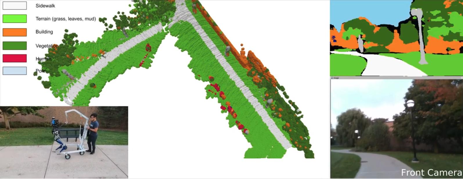
Figure 1: Building a semantic map for autonomous navigation. Once the transformation from LiDAR to camera is known, it is possible to fuse the LiDAR and RGB-camera information to build a 3D-map that is annotated with semantic information. The lower right shows a single camera image; its segmentation with semantic labels is shown in the upper right. Synchronized LiDAR points are mapped onto the camera image, associated to a semantic label, and then re-projected to a local frame [25] along with the semantic labels to create a 3D semantically-labeled map [1], shown in the upper left. The sidewalk is marked in white, the grass in yellow-green, and trees in dark green. In the lower left, Cassie is using the map to plan a path around the North Campus Wave Field, while staying on the sidewalk.

The two most common sets of features in the area of target-based calibration are (a) the 3D-coordinates of the vertices of a rectangular or triangular planar target, and (b) the normal vector to the plane of the target and the lines connecting the vertices in the plane of the target. Mathematically, these two sets of data are equivalent: knowing one of them allows the determination of the other. In practice, focusing on (b) leads to use of the SVD to find the normal vector and more broadly to least squares line fitting problems [24], while (a) opens up other perspectives, as highlighted in [23].

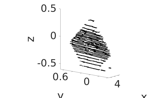
(a)

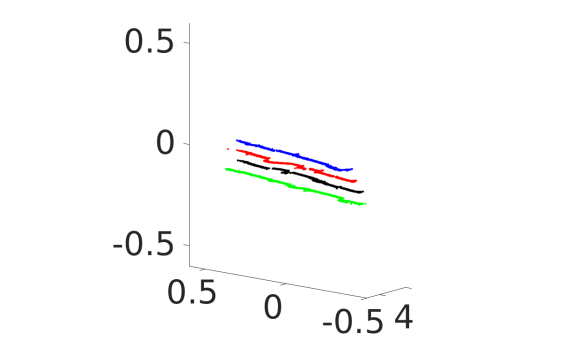
(b)

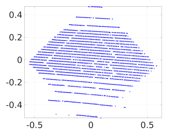
(c)

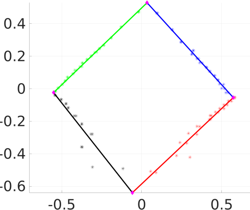
(d)

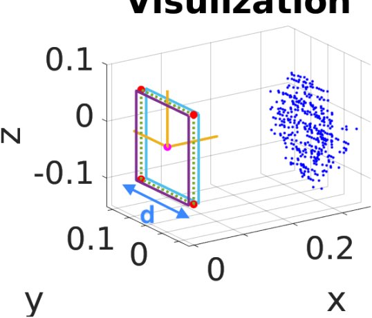
(e)

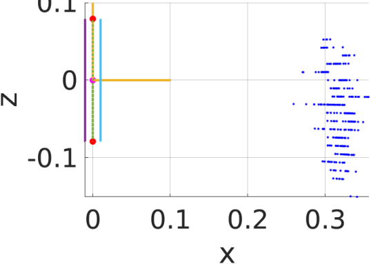
(f)

Figure 2: Units are meters. LABEL:sub@fig:FigureLiDARScanExample Twenty five LiDAR scans of a planar target. The point cloud is roughly 7 cm thick. LABEL:sub@fig:FigureLiDARScanExample3Rings The “noise” in the point cloud is not random. A zoom for four of the rings (13, 15, 17, 19) is typical and shows systematic errors in distance. LABEL:sub@fig:payload2D LiDAR  points orthogonally projected to the plane defined by the normal. LABEL:sub@fig:payload_LN2D Example edge points selected to regress a line via RANSAC. LABEL:sub@fig:reference_frame Target reference frame and real point cloud data. The dotted blue square is the reference target; its vertices are denoted $\{\bar{X}_{i}\}_{i=1}^{4}$. LABEL:sub@fig:reference_frame_side A side-$(x-z)$-view highlighting the non-zero thickness of a typical point cloud. These figures and all others in the paper are of sufficient resolution that they can be blown up to see detail.

Figure 2a shows a 3D view of 25 scans from a factory-calibrated 32-Beam Velodyne ULTRA Puck LiDAR on a diamond shaped planar target. The zoom provided in Fig. 2b shows that some of the rings are poorly calibrated, with a “noise level” that is three times higher than the manufacturer’s specification. On average, the rings are close to the specification ($\pm$ five cm at less than 50 m) of the LiDAR, which means a maximum ten centimeters difference between points on the same ring.

Systematic errors in the distance (or depth) measurement affect the estimation of the target’s centroid, which is commonly used to determine the translation of the target with respect to the LiDAR, and the target’s normal vector, which is used to define the plane of the target, as shown in Fig. 2c. Subsequently, the point cloud is orthogonally projected to this plane and the line boundaries of the target are found by performing RANSAC on the appropriate set of ring edges; see Fig. 2d. The lines along the target’s boundaries then define its vertices in the plane, which for later reference, we note are not constrained to be compatible with the target’s geometry.

Once the vertices in the plane of the target have been determined, then knowledge of the target’s normal vector allows the vertices to be lifted back to the coordinates of the point cloud. This process may be repeated for multiple scans of a target, aggregates of multiple scans of a target, or several targets, leading to a list of target vertices $\{X_{i}\}_{i=1}^{4n}$, where $n$ is the number of target poses.

The target is typically designed so that the vertices are easily distinguishable in the camera image. Denoting their corresponding coordinates in the image plane by $\{Y_{i}\}_{i=1}^{4n}$ completes the data required for the conceptual fitting problem in (1). While the cost to be minimized is nonlinear and non-convex, this is typically not a problem because CAD data can provide an adequate initial guess for local solvers, such as Levenberg-Marquardt; see [24] for example.

I-B Our Contributions

Our contributions can be summarized as follows.

1. We introduce a novel method for estimating the rigid-body transform from target to LiDAR, $H_{T}^{L}$. For the point cloud pulled back to the origin of the LiDAR frame via the current estimate of the transformation, the cost is defined as the sum of the distance of a point to a 3D-reference target of known geometry in the LiDAR frame, for those points landing outside of the reference target, and zero otherwise. We use an $L_{1}$-inspired norm in this work to define distance. Consistent with [23], we find that this is less sensitive to outliers than $L_{2}$-line fitting to edge points using RANSAC [24].

2. In the above, by using the entire target point cloud when estimating the vertices, we avoid all together the delicate task of identifying the edge points and parsing them into individual edges of the target, where small numbers of points on some of the edges accentuate the quantization effects due to sparsity in a LiDAR point cloud.

3. We provide a round-robin validation study to compare our approach to a state-of-the-art method, namely [24]. A novel feature of our validation study is the use of the camera image as a proxy for ground truth; in the context of 3D semantic mapping, this makes sense. In addition to a standard PnP method [22] for estimating the rigid-body transformation from LiDAR to camera, we also investigate maximizing intersection over union (IoU) to estimate the rigid-body transformation. Our algorithms are validated on various numbers of targets.

4. Code for our method, our implementation of the baseline, and all the data sets used in this paper are released as open source; see [26].

II Finding the LiDAR Target Vertices

We assume that each target is planar, square, and rotated in the frame of the LiDAR by roughly 45^∘ to form a diamond as in Fig. 2a. As indicated in [23, 24], placing the targets so that the rings of the LiDAR run parallel to its edges leads to ambiguity in the vertical position due to the spacing of the rings. We assume that standard methods have been used to automatically isolate the target’s point cloud [27] and speak no further about it.

We take as a target’s features its four vertices, with their coordinates in the LiDAR frame denoted $\{X_{i}\}_{i=1}^{4};$ when useful, we abuse notation and pass from ordinary coordinates to homogeneous coordinates without noting the distinction. The vertices $\{X_{i}\}_{i=1}^{4}$ are of course not directly observable in the point cloud. This section will provide a new method for estimating their coordinates in the frame of the LiDAR using an $L_{1}$-like norm.

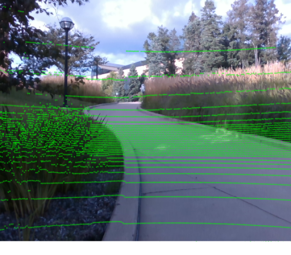
(a)

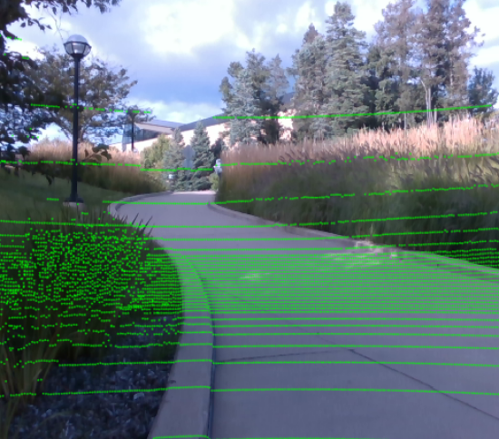
(b)

Figure 3: LABEL:sub@fig:disturbance shows that a calibration result is not usable if it has a few degrees of rotation error and a few percent of translation error. LABEL:sub@fig:undisturbance shows good alignment of a LiDAR  point cloud projected onto a camera image.

II-A Remarks on LiDAR Point Clouds

LiDARs have dense regions and sparse regions along the z-axis, as shown in Fig. 2c. For a 32-beam Velodyne Ultra Puck, we estimate the resolution along the z-axis is $0.33^{\circ}$ and $1.36^{\circ}$ in the dense and sparse regions, respectively. A point’s distance resolution along the y-axis is roughly $0.1^{\circ}$. The quantization error could be roughly computed from: $d\sin{\theta}$ when a point is at $d$ meter away. As a result, the quantization error could get quite large if one place the tag at a far distance. Figure 3a shows that a $1^{\circ}$ of rotation error on each axis and 5% error in translation can significantly degrade a calibration result. As noted in [23, 24], it is essential to place a target at an appropriate angle so that known geometry can mitigate quantization error in the $y$- and $z$-axes.

II-B New Method for Determining Target Vertices

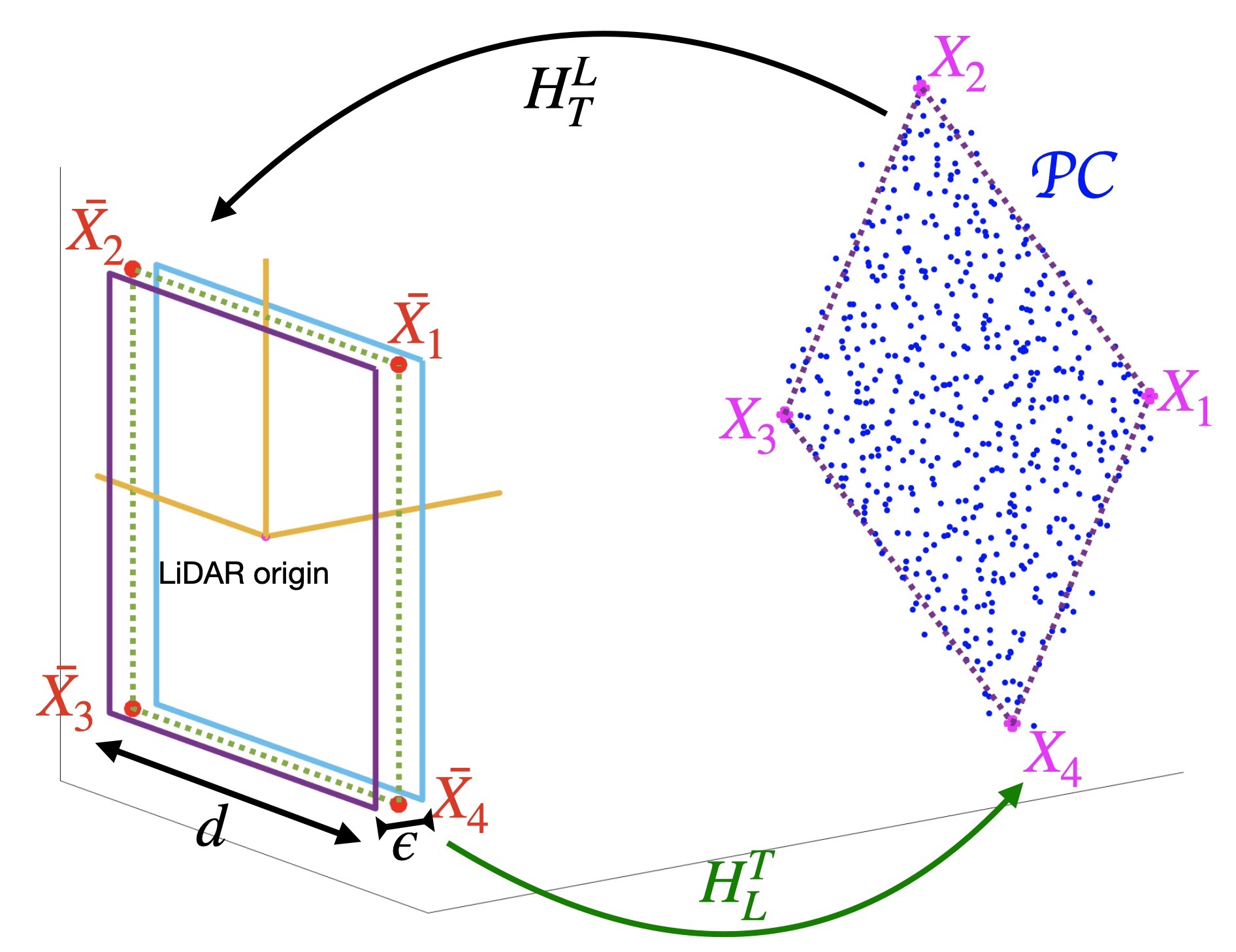
Figure 4: This conceptual figure illustrates the proposed method to estimate LiDAR vertices. The target’s reference in the LiDAR frame is defined by ($\bar{X_{1}},\cdots,\bar{X_{4}}$) with depth $\epsilon$. The rigid-body transformation $H_{T}^{L}$ (black arrow) pulls back the target’s $\mathcal{PC}$ to a target reference about the LiDAR origin. The actual vertices ($X_{1},\cdots,X_{4}$) of the target are estimated by (5), using the inverse transformation $H_{L}^{T}$ (green arrow).

Let ${\cal PC}$ denote the LiDAR point cloud of the target and let the collection of 3D points be ${\cal X}_{i}$ so that ${\cal PC}=\{{\cal X}_{i}\}_{i=1}^{N}$, where $N$ is the number of points on the target. For the extrinsic calibration problem, we need to estimate the target vertices in the LiDAR frame. As in Fig. 4, let $H_{L}^{T}$ be the rigid-body transformation from a reference target in the LiDAR frame with vertices $\{\bar{X}_{i}\}_{i=1}^{4}$, onto the point cloud. We use the inverse transform $H_{T}^{L}:=(H_{L}^{T})^{-1}$ to pull back the target’s point cloud to the origin of the LiDAR and measure the error there.

For $a\geq 0$ and $\lambda\in\mathbb{R}$, define

$$c(\lambda,a):=\begin{cases}\min\{|\lambda-a|,|\lambda+a|\}&\text{if}~{}|\lambda|>a\\ 0&\text{otherwise}\end{cases};$$ (2)

see also the “soft $L_{1}$ norm” in [23]. Let $\{\tilde{{\cal X}}_{i}\}_{i=1}^{N}:=H_{T}^{L}(\mathcal{PC}):=\{H_{T}^{L}({\cal X}_{i})\}_{i=1}^{N}$ denote the pullback of the point cloud by $H_{T}^{L}$, and denote a point’s Cartesian coordinates by $(\tilde{x}_{i},\tilde{y}_{i},\tilde{z}_{i})$. The cost is defined as

$$C(H_{T}^{L}(\mathcal{PC})):=\sum_{i=1}^{N}c(\tilde{x}_{i},\epsilon)+c(\tilde{y}_{i},d/2)+c(\tilde{z}_{i},d/2),$$ (3)

where $d$ is determined by the size of the (square) target, and the only tuning parameter is $\epsilon>0$, the thickness of the ideal target. The value of $\epsilon$ is based on the standard deviation of a target’s return points to account for the noise level of the depth measurement; see Fig. 2f.

We propose to determine the optimal rigid-body transformation, with rotation matrix $R_{T}^{L}$ and translation vector $T_{T}^{L}$, by

$$H_{T}^{L^{*}}:=\operatorname*{arg\,min}_{R_{T}^{L},T_{T}^{L}}C(H_{T}^{L}(\mathcal{PC})),$$ (4)

and to define the estimated target vertices by

$$X_{i}^{*}:=H_{L}^{T^{*}}(\bar{X}_{i}),~{}~{}1\leq i\leq 4.$$ (5)

Remark 1.

It is emphasized that the target vertices are being determined without extraction of edge points and their assignment to a side of the target. The correspondences of the estimated vertices with the physical top, bottom, and left or right sides of the target are not needed at this point.

Remark 2.

The cost in (3) treats the target as a rectangular volume. To be clear, what we seek is a “best estimate” of the target vertices in the LiDAR frame and not the transformation itself. Our method is indirect because from the point cloud, we estimate a “best” LiDAR to target transformation, $H_{L}^{T^{*}}$, and use it to define the vertices by (5).

III Image Plane Corners and Correspondences with the LiDAR Vertices

For a given camera image of a LiDAR target, let $\{{}_{C}Y_{i}\}_{i=1}^{4}$ denote the corners of the camera image. We assume that these have been obtained through the user’s preferred method, such as corner detection [28, 29, 30], edge detection [31, 32, 33], or even manual selection. The resulting camera corners are used in both the proposed method and the baseline. This is not the hard part of the calibration problem. To achieve simple correspondences $X_{i}\leftrightarrow{}_{C}Y_{i}$, the order of the indices of $\{X_{i}\}_{i=1}^{4}$ may need to be permuted; we use the vertical and horizontal positions to sort them; see [26].

Once we have the correspondences, the next step is to project the vertices of the LiDAR  target, $\begin{bmatrix}x_{i}&y_{i}&z_{i}&1\end{bmatrix}^{\mathsf{T}}=X_{i}$, into the image coordinates. The standard relations are [34, 35]

$$\begin{bmatrix}u^{\prime}\\ v^{\prime}\\ w^{\prime}\end{bmatrix} =\begin{bmatrix}f_{x}&s&c_{x}\\ 0&f_{y}&c_{y}\\ 0&0&1\end{bmatrix}\begin{bmatrix}\mathbb{1}_{3\times 3}\\ \textbf{0}_{1\times 3}\end{bmatrix}^{\mathsf{T}}\begin{bmatrix}R_{L}^{C}&T_{L}^{C}\\ \textbf{0}_{1\times 3}&1\\ \end{bmatrix}\begin{bmatrix}x_{i}\\ y_{i}\\ z_{i}\\ 1\end{bmatrix}$$ (6)

$${}_{L}Y_{i} =\begin{bmatrix}u&v&1\end{bmatrix}^{\mathsf{T}}=\begin{bmatrix}\frac{u^{\prime}}{w^{\prime}}&\frac{v^{\prime}}{w^{\prime}}&1\end{bmatrix}^{\mathsf{T}},$$ (7)

where (6) includes the camera’s intrinsic parameters and the extrinsic parameters $(R_{L}^{C},T_{L}^{C})$ that we seek.

For later use, we combine (6) and (7) to define

$$\Pi\left(X_{i};R_{L}^{C},T_{L}^{C}\right):={}_{L}Y_{i},$$ (8)

the projection map from LiDAR coordinates to image coordinates. Note that it is a function of both the extrinsic variables and the LiDAR vertices.

IV Extrinsic Transformation Optimization

This section assumes the vertices of the target in the LiDAR frame and in the camera’s image plane have been determined, along with their correspondences. The optimization for the extrinsic transformation can be formulated in a standard PnP problem: minimize Euclidean distance of the corresponding corners. We also propose maximizing the intersection over union (IoU) of the corresponding projected polygons.

IV-A Euclidean distance

The standard PnP formulation is

$$\left({R_{L}^{C}}^{*},{T_{L}^{C}}^{*}\right) :=\operatorname*{arg\,min}_{R,T}\sum_{i=1}^{4n}\left\lVert\Pi\left(X_{i};R,T\right)-{}_{C}Y_{i}\right\rVert_{2}^{2}$$

$$=\operatorname*{arg\,min}_{R,T}\sum_{i=1}^{4n}\left\lVert{}_{L}Y_{i}-{}_{C}Y_{i}\right\rVert_{2}^{2},$$ (9)

where ${}_{C}Y_{i}\in\mathbb{R}^{2}$ are the camera corners, ${}_{L}Y_{i}\in\mathbb{R}^{2}$ are defined in (8), and $n$ is the number of target poses.

IV-B IoU optimization

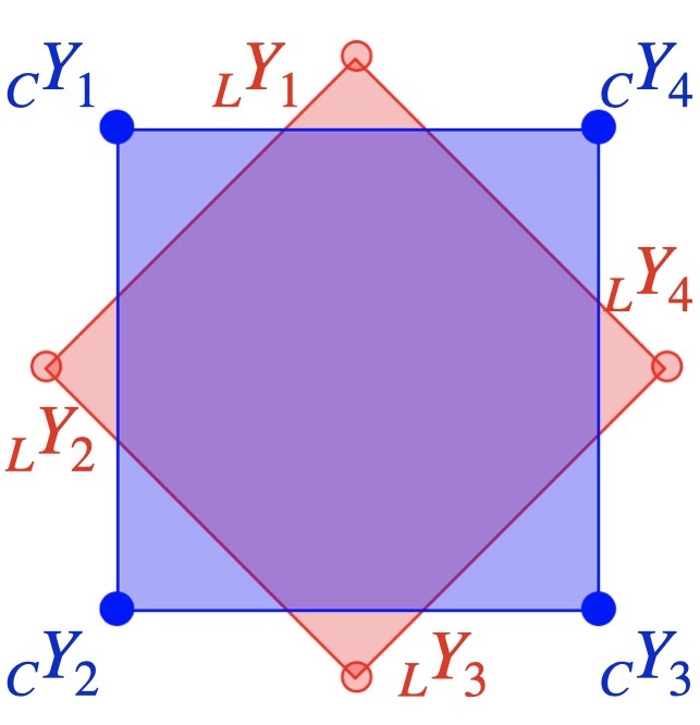
(a)

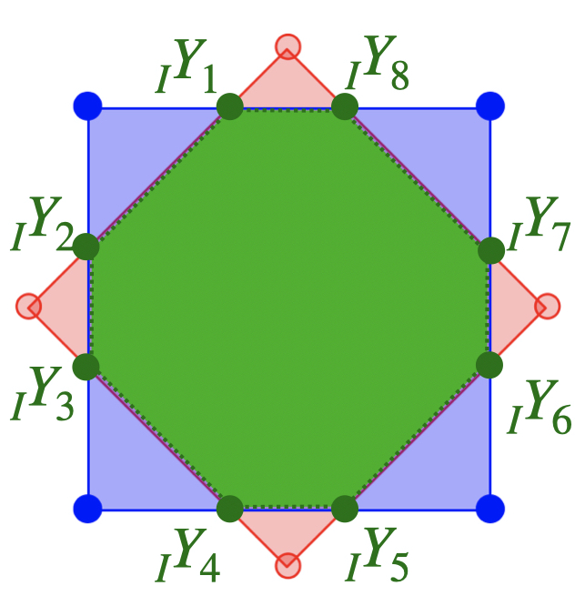
(b)

Figure 5: Two polygons in an image plane. LABEL:sub@fig:TwoPolygons the red polygon ${}_{L}\mathcal{V}=\{{}_{L}Y_{i}\}_{i=1}^{4}$ represents the estimated vertices projected from the LiDAR frame to the image plane, while the blue polygon ${}_{C}\mathcal{V}=\{{}_{C}Y_{i}\}_{i=1}^{4}$ represents the vertices of the actual camera image of the target. LABEL:sub@fig:IntersectionPolygon shows the intersection (marked in green) of the two polygons, with the vertices labeled as ${}_{I}\mathcal{V}=\{{}_{I}Y_{i}\}_{i=1}^{8}$.

For a given polygon, let $\mathcal{V}:=\{Y_{i}|Y_{i}=:(x_{i},~{}y_{i})\}_{i=1}^{N}$ be the coordinates of the $N$ vertices, ordered counterclockwise. The area of the polygon is computed via the Shoelace algorithm [36, eq. (3.1)] [37],

$$\textbf{A}(\mathcal{V})=\textbf{A}(Y_{1},\cdots,Y_{N})=\frac{1}{2}\left|\sum_{i=1}^{N}\det\begin{bmatrix}x_{i}&x_{i+1}\\ y_{i}&y_{i+1}\end{bmatrix}\right|,$$ (10)

where $x_{N+1}:=x_{1}$ and $y_{N+1}:=y_{1}$. If $\mathcal{V}$ is empty, the area is taken as zero. We now apply this basic area formula to propose an IoU-based cost function for extrinsic calibration.

Let ${}_{L}\mathcal{V}:=\{{}_{L}Y_{i}\}_{i=1}^{4n}$ be the vertices of the estimated target polygons projected from the LiDAR frame to the camera frame as in (8), and let ${}_{C}\mathcal{V}:=\{{}_{C}Y_{i}\}_{i=1}^{4n}$ be the vertices of the corresponding camera images of the targets, as in Fig. 5a. If their intersection is nonempty, we define it as a polygon with known coordinates, denoted as ${}_{I}\mathcal{V}:=\{{}_{I}Y_{i}\}_{i=1}^{M}$, where $M\geq 0$ is the number of intersection points; see Fig. 5b. We sort the three sets of vertices of the polygons counterclockwise using Graham’s scan algorithm, a method to find the convex hull of a finite set of points in a plane [38, 39]. The IoU of the two polygons is then

$$IoU({}_{L}\mathcal{V},{}_{C}\mathcal{V},{}_{I}\mathcal{V})=\frac{\textbf{A}({}_{I}\mathcal{V})}{\textbf{A}({}_{L}\mathcal{V})+\textbf{A}({}_{C}\mathcal{V})-\textbf{A}({}_{I}\mathcal{V})}.$$ (11)

The resulting optimization problem is

$$\left({R_{L}^{C}}^{*},{T_{L}^{C}}^{*}\right) :=\operatorname*{arg\,max}_{R,T}IoU({}_{L}\mathcal{V},{}_{C}\mathcal{V})$$ (12)

$$=\operatorname*{arg\,max}_{R,T}IoU(\Pi\left(\{X_{i}\}_{i=1}^{4n};R,T\right),{}_{C}\mathcal{V}),$$

where (8) has been used to make the dependence on the rigid-body transformation explicit.

V Experimental Results

In this section, we extensively evaluate our proposed method on seven different scenes through a form of “cross-validation”: in a round-robin fashion, we estimate an extrinsic transformation using data from one or more scenes and then evaluate it on the remaining scenes. The quantitative evaluation consists of computing pixel error per corner, where we take the image corners as ground truth. We also show qualitative validation results by projecting the LiDAR scans onto camera images; we include here as many as space allows, with more scenes and larger images available at [26].

V-A Data Collection

The scenes include both outdoor and indoor settings. Each scene includes two targets, one approximately 80.5 cm square and the other approximately 15.8 cm square, with the smaller target placed closer to the camera-LiDAR pair. We use an Intel RealSense Depth Camera D435 and a 32-Beam Velodyne ULTRA Puck LiDAR, mounted on an in-house designed torso for a Cassie-series bipedal robot [3]. From the CAD file, the camera is roughly 20 cm below the LiDAR and 10 cm in front of it. The angle of the camera is adjustable. Here, its “pitch”, in the LiDAR frame, is approximately zero.

A scan consists of the points collected in one revolution of the LiDAR’s 32 beams. The data corresponding to a single beam is also called a ring. For each scene, we collect approximately 10 s of synchronized data, resulting in approximately 100 pairs of scans and images.

For each target, five consecutive pairs of LiDAR scans and camera images are selected as a data set. For each data set, we apply two methods to estimate the vertices of the targets, a baseline and the method in Sec. II-B. We then apply both PnP and IoU optimizations to find the rigid-body transformation, see Sec. IV.

V-B Baseline Implementation for LiDAR Vertices

As a baseline, we use the method in [24]. Because an open-source implementation was not released, we built our own, attempting to be as faithful as possible to the described method.

For each scan, the large and small targets are individually extracted from background [27]. For each target and group of five scans, we compute the extracted point cloud’s centroid and center the point cloud about the origin. SVD is then used to find the target’s normal and to orthogonally project the point cloud onto the plane defined by the normal and the centroid. For each scan, and for each ring hitting the target, the left and right end points of the ring are selected and then associated with one of the four edges of the target. Lines are fitted to each collection of edge points using least-squares and RANSAC. The vertices are obtained as the intersections of the lines in the plane defined by the target’s normal and centroid. The four vertices are then re-projected to 3D space, as in Fig. 2d.

V-C Camera Corners and Associations

The process of determining the target corners begins by clicking near them in the image. This is the only manual intervention required in the paper and even this process will soon be automated. As shown in Fig. 6a, between any given two clicked points, i.e., an edge of the target, a bounding box is drawn around the two points. Once we have roughly located the corners of the target, we process the image with Canny edge detection to detect the edge points within the bounding box. A line is then fit through each edge using RANSAC, and the intersections of the resulting lines define the target’s corners, as shown in Fig. 6b. A video and an implementation of this process is released along with the code.

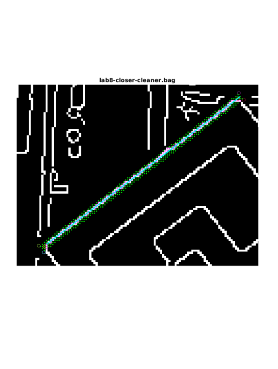
(a)

(b)

Figure 6: LABEL:sub@fig:Cannyedges shows the result of edge detection. LABEL:sub@fig:CannyLineFitted shows the interior pixels (marked in green) of a bounding box given two clicked corners. The edge points and the edge line (as found by RANSAC) are marked in magenta and cyan, respectively. The corners are defined by the intersections of the resulting lines.

V-D Extrinsic Calibration

On the basis of the associated target vertices and camera-image corners, both the PnP and IoU methods are used to find the rigid-body transformation from LiDAR to camera. Because the results are similar, we report only the PnP method in Table I and then include both in the summary table (Table II). SVD and RANSAC were computed using their corresponding MATLAB commands, while the optimizations in (4), (IV-A) and (12) were done with fmincon.

V-E Computation Performance

The calibration is done offline. The round-robin cross-validation study given in Table I was generated in MATLAB in less than an hour. Each dataset (including the baseline and the proposed method) takes about 1.5 minutes in MATLAB.

V-F Quantitative Results and Round-robin Analysis

In Table I, we present the RMS error of the LiDAR vertices projected into the camera’s image plane for the baseline, labeled RANSAC-normal (RN), and our method in (3) and (4), labeled geometry-L₁ (GL₁). In the case of two targets, a full round-robin study is performed: the rigid-body transformation from LiDAR to camera is “fit” to the combined set of eight vertices from both targets and then “validated” on the eight vertices of each of the remaining six scenes.

A complete round-robin study for four targets from two scenes would require 21 validations, while for six and eight targets, 35 validations each would be required. For space reasons, we report only a subset of these possibilities.

To be clear, we are reporting in units of pixel per corner

where $4n$ is the total number of target corners. In the case of two targets and one scene, $n=2$. In the case of six targets from three scenes, $n=6$. Figure 7 illustrates several point clouds projected to the corresponding camera images. Summary data is presented in Table II.

TABLE I: Fitting and validation data. The gray boxes denote the fitting set and the white boxes contain validation data. The numbers are the RMS errors of the LiDAR vertices projected to the image plane, measured in units of pixels per corner; see (13). For two targets, a complete round-robin study was done. For more targets, the number of combinations became prohibitive. S₁ through S₇ denote scene (experiment) number. The mean and standard deviation of each row—excluding the fitting set—are given in the last two columns.

Fitting\Validation	Method	# Tag	S1	S2	S3	S4	S5	S6	S7	mean	std
	RN	2	2.6618	8.7363	4.4712	7.3851	4.1269	7.1884	11.9767	7.3141	2.8991
S1	GL1	2	0.7728	2.3303	2.3230	1.6318	1.3694	1.9637	2.7427	2.0602	0.5055
	RN	2	3.3213	7.6645	4.9169	5.2951	4.0811	4.4345	7.7397	4.9648	1.5215
S2	GL1	2	2.1368	1.5181	3.2027	3.2589	2.4480	4.1563	4.4254	3.2713	0.9039
	RN	2	4.9909	9.5620	3.6271	8.7533	4.6421	10.1308	15.7764	8.9759	4.0654
S3	GL1	2	4.6720	5.9350	1.8469	6.9331	4.4352	8.9493	15.3862	7.7185	4.1029
	RN	2	21.2271	22.1641	17.5779	2.9452	15.9909	8.8797	15.3636	16.8672	4.7833
S4	GL1	2	4.3681	4.7176	4.4804	0.4986	3.9004	3.3891	3.7440	4.0999	0.5040
	RN	2	3.4621	8.3131	4.8500	7.6217	3.5197	7.4838	12.4364	7.3612	3.1066
S5	GL1	2	2.0590	2.9541	3.0224	3.5483	0.7392	3.1386	6.0885	3.4685	1.3733
	RN	2	29.4400	27.5404	27.9955	9.7005	20.6511	1.4253	9.5050	20.8054	9.1941
S6	GL1	2	5.1207	5.0574	5.3537	2.0539	4.1739	1.0012	2.4194	4.0298	1.4503
	RN	2	7.7991	9.9647	7.6857	4.1640	6.1619	2.3398	2.3708	6.3525	2.7512
S7	GL1	2	2.1563	2.7837	3.1058	1.3234	2.4537	2.0838	1.5389	2.3178	0.6207
	RN	4	6.9426	9.6281	6.9136	3.9650	5.6420	2.2399	2.2399	6.6183	2.0764
S6-S7	GL1	4	2.2409	2.5607	2.9773	1.8215	2.1995	0.3417	0.3417	2.3600	0.4334
	RN	4	4.2476	8.5054	4.6712	2.8686	4.3311	2.8686	2.8748	4.9260	2.1153
S4-S6	GL1	4	1.0746	1.8871	2.3619	0.2341	1.5350	0.2341	2.6191	1.8955	0.6215
	RN	4	2.9309	8.0801	4.1196	3.4985	3.1519	3.1519	3.2204	4.3699	2.1201
S5-S6	GL1	4	1.1541	2.1026	2.5017	1.4267	0.3291	0.3291	2.5693	1.9509	0.6361
	RN	4	3.1991	6.0812	4.7311	5.4558	6.0812	4.8344	8.6576	5.3756	2.0139
S2-S5	GL1	4	0.9538	0.4803	2.3810	1.4556	0.4803	1.1592	2.5277	1.6955	0.7172
	RN	4	2.8820	6.2167	6.2167	4.4672	3.9536	3.7802	6.2324	4.2631	1.2406
S2-S3	GL1	4	1.0896	0.4826	0.4826	1.5349	1.5938	1.5597	2.7543	1.7065	0.6209
	RN	4	2.8595	8.2471	4.3297	3.7712	4.1023	2.4679	2.8595	4.5836	2.1710
S1-S7	GL1	4	1.3542	1.9973	2.3987	1.5926	1.4978	1.6130	1.3542	1.8199	0.3757
	RN	4	2.5633	8.0573	4.1762	3.6859	3.8973	2.5633	3.2569	4.6147	1.9535
S1-S6	GL1	4	0.9753	1.9154	2.3361	1.2906	1.2827	0.9753	2.3205	1.8291	0.5231
	RN	6	2.9824	8.0943	4.1273	3.2821	3.2821	3.2821	3.0841	4.5720	2.4045
S4-S5-S6	GL1	6	0.9713	1.9887	2.4395	0.3288	0.3288	0.3288	2.4369	1.9591	0.6918
	RN	6	2.7816	5.5382	5.5382	4.5817	5.5382	3.8262	6.6229	4.4531	1.6239
S2-S3-S5	GL1	6	1.0022	0.4712	0.4712	1.4755	0.4712	1.1722	2.7791	1.6073	0.8054
	RN	6	3.3906	8.1677	3.3906	3.6688	3.9558	2.2913	3.3906	4.5209	2.5374
S1-S3-S7	GL1	6	1.7666	1.9994	1.7666	1.5854	1.4754	1.5124	1.7666	1.6432	0.2419
	RN	6	2.9428	5.5357	5.5357	5.5357	3.8913	2.4828	3.7673	3.2711	0.6733
S2-S3-S4	GL1	6	0.9523	1.8195	1.8195	1.8195	1.5275	1.3631	2.4347	1.5694	0.6255
	RN	6	5.3281	5.3281	5.3281	4.5086	3.8577	3.7165	6.4413	4.6310	1.2552
S1-S2-S3	GL1	6	1.7755	1.7755	1.7755	1.3698	1.4807	1.3422	2.3156	1.6271	0.4629
	RN	6	3.2743	8.2067	4.2628	3.5584	3.0628	3.0628	3.0628	4.8256	2.2921
S5-S6-S7	GL1	6	0.9594	2.0149	2.3877	1.3754	1.4905	1.4905	1.4905	1.6843	0.6390
	RN	8	3.5316	8.1362	3.5316	3.4616	3.5316	2.2642	3.5316	4.6207	3.1029
S1-S3-S5-S7	GL1	8	1.6904	1.9886	1.6904	1.4743	1.6904	1.4136	1.6904	1.6255	0.3159
	RN	8	4.9240	4.9240	4.2049	3.6159	4.9240	2.2928	4.9240	3.3712	0.9793
S1-S2-S5-S7	GL1	8	1.5269	1.5269	2.4070	1.4788	1.5269	1.4650	1.5269	1.7836	0.5399
	RN	8	3.6113	8.0593	3.6113	3.6113	3.6113	2.4532	3.8397	4.7841	2.9199
S1-S3-S4-S5	GL1	8	1.4986	2.0563	1.4986	1.4986	1.4986	1.2256	2.6797	1.9872	0.7295
	RN	8	3.0803	5.0057	4.1893	5.0057	5.0057	2.3307	5.0057	3.2001	0.9351
S2-S4-S5-S7	GL1	8	0.9530	1.5921	2.4280	1.5921	1.5921	1.4865	1.5921	1.6225	0.7469

TABLE II: A summary of validation data in Table I. This table compares mean and standard deviation for baseline and our approach as a function of the number of targets used in fitting. Units are pixel per corner.

Method	# Tag	2	4	6	8
Baseline-RN	mean	10.3773	4.9645	4.3789	3.9940
GL1-PnP	mean	3.8523	1.8939	1.6817	1.7547
GL1-IoU	mean	4.9019	2.2442	1.7631	1.7837
Baseline-RN	std	7.0887	1.9532	1.7771	2.0467
GL1-PnP	std	2.4155	0.5609	0.5516	0.5419
GL1-IoU	std	2.5060	0.7162	0.5070	0.4566

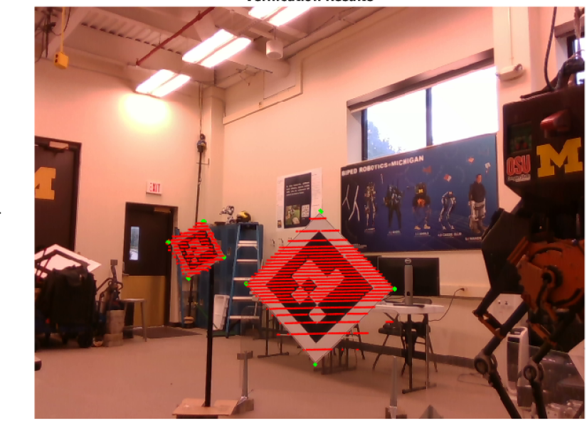
(a)

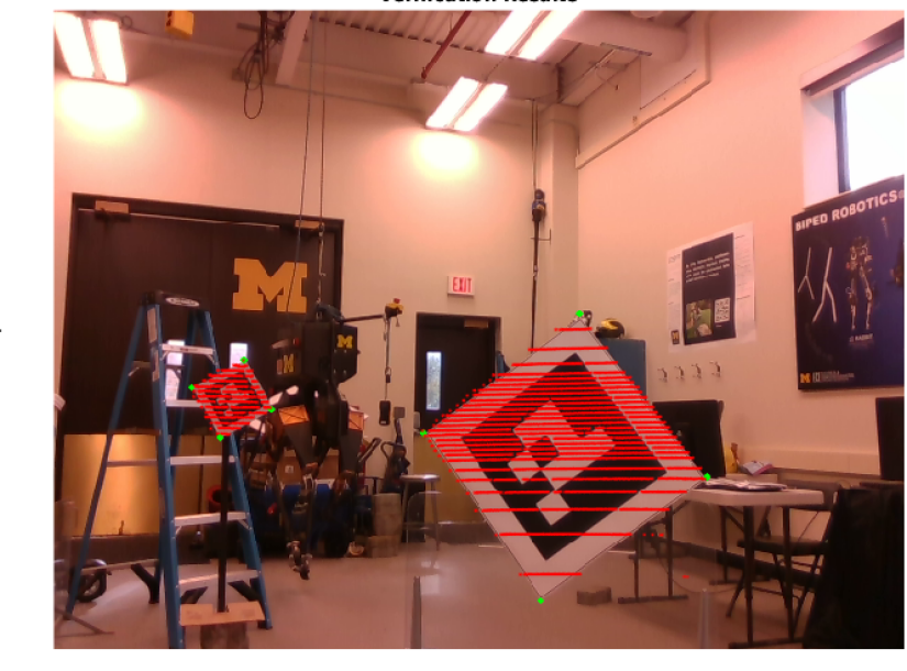
(b)

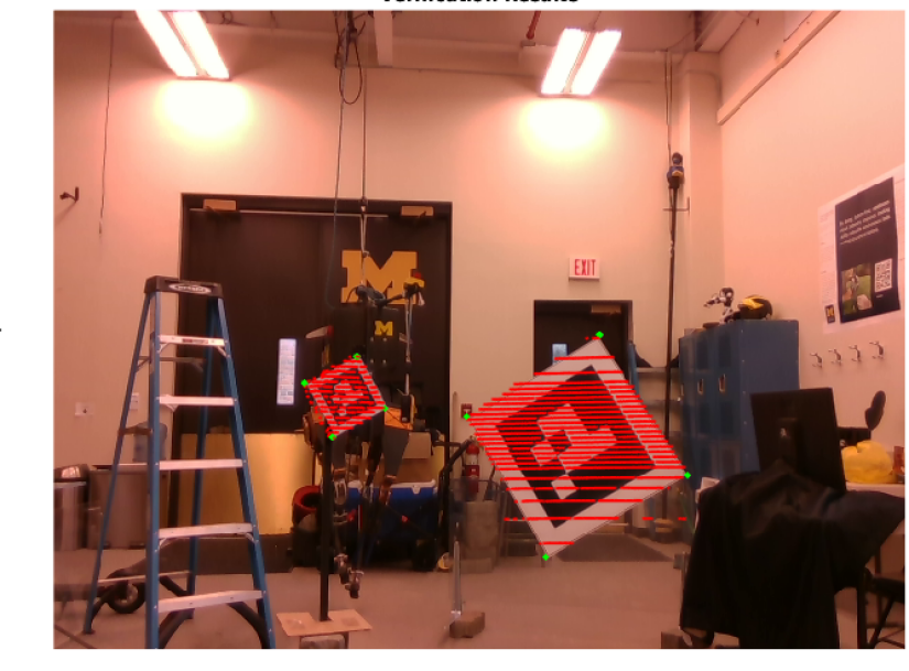
(c)

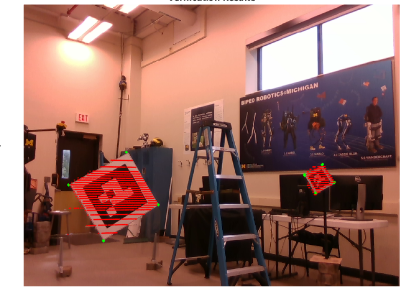
(d)

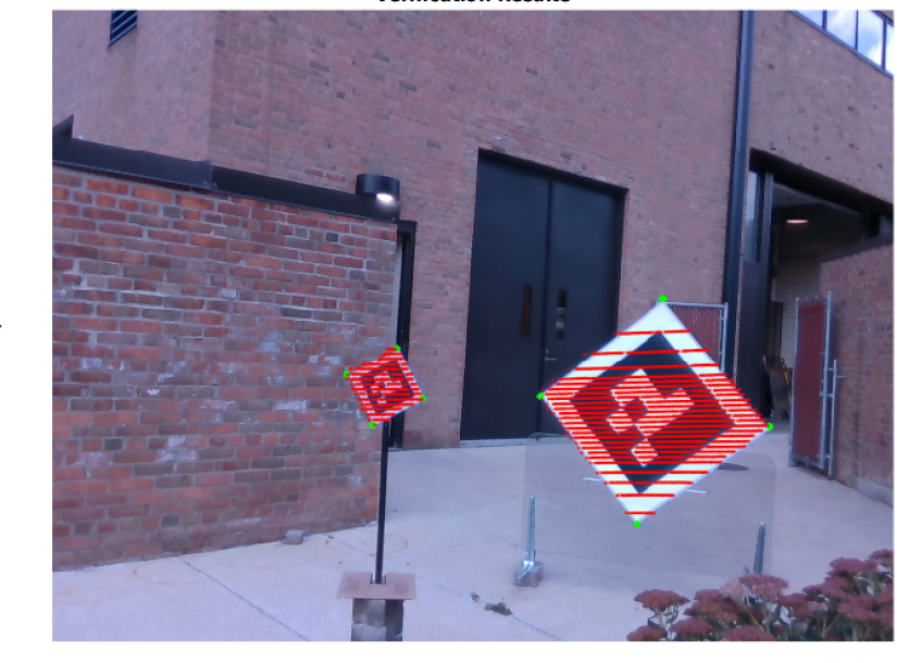
(e)

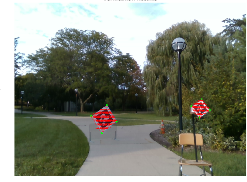
(f)

Figure 7: Visual depiction of the validation data in the last row of Table I. For the method GL₁, five sets of estimated LiDAR vertices for each target have been projected into the image plane and marked in green, while the target’s point cloud has been marked in red. Blowing up an image allows the numbers reported in the table to be visualized. The vertices are key.

VI Qualitative Results and Discussion

In LiDAR to camera calibration, due to the lack of ground truth, it is common to show projections of LiDAR point clouds onto camera images. Often it is unclear if one is viewing fitting data or validation data. In Figure 8, we show a set of projections of LiDAR point clouds onto camera images for validation data. An additional set of images can be found in [26]. All of them show that the key geometric features in the image and point cloud are well aligned. The quality of the alignment has allowed our laboratory to build a high-quality (real-time) 3D semantic map with our bipedal robot Cassie Blue [40]. The map fuses LiDAR, camera, and IMU data; with the addition of a simple planner, it led to autonomous navigation [41].

Tables I and II show that GL₁ outperforms the baseline: on average, there is more than a 50% reduction in projection error and a 70% reduction in its variance. As for the sources of this improvement, we highlight the following points:

1. Least-squares-based methods estimate a normal vector for the target’s point cloud. As shown in Fig. 2a and Fig. 2b, even though the target is flat and has a well-defined normal, the returns in the LiDAR point cloud do not lie on a plane. Hence, a global normal vector does not exist.

2. Least-squares-based methods extract the target edge points from the point cloud for use in line fitting. The line fitting must be done in the plane defined by the estimated normal because, in 3D, non-parallel lines do not necessarily intersect to define a vertex.

3. GL₁ explicitly uses the target geometry in formulating the cost function. By assigning zero cost to interior points in the “ideal target volume” and non-zero otherwise, the optimization problem is focused on orienting the boundary of the target volume within the 3D point cloud. This perspective seems not to have been used before.

4. Hence, our approach does not require the (tedious and error-prone) explicit extraction and assignment of points to target edges. The determination of boundary points in 3D is implicitly being done with the cost function.

At the present time, our extrinsic calibration method is not “automatic”. The one manual intervention, namely clicking on the approximate target corners in the camera image, will be automated soon.

We have not conducted a study on how to place the targets. This is an interesting piece of future work because of the nonlinear operation required when projecting LiDAR points to the camera plane; see (6) and (7).

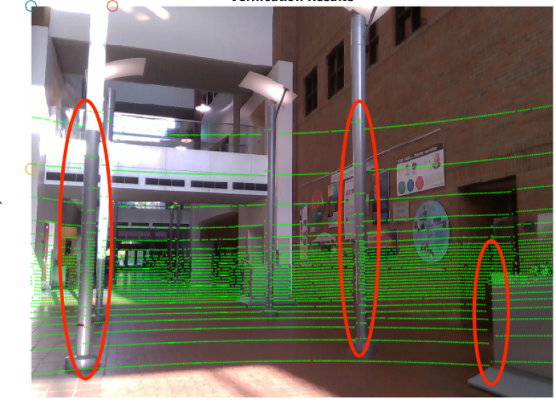
(a)

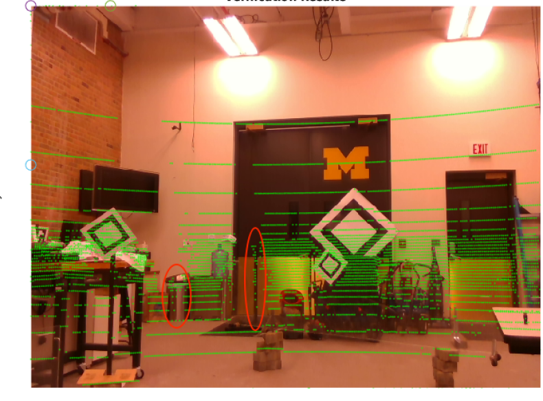
(b)

(c)

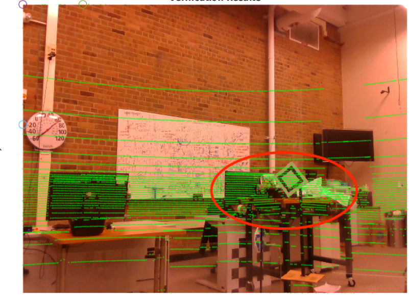
(d)

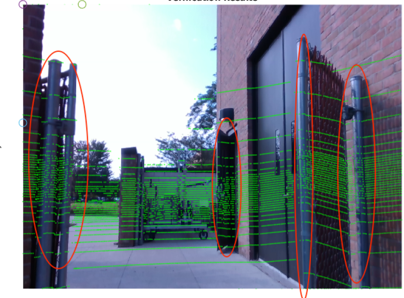
(e)

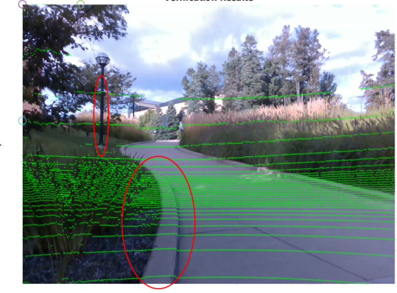
(f)

Figure 8: Qualitative validation results. Using the extrinsic transformation obtained by the method GL₁ applied to S₁, the LiDAR point cloud has been projected into the image plane for the other data sets and marked in green. The red circles highlight various poles, door edges, desk legs, monitors, and sidewalk curbs where the quality of the alignment can be best judged. The reader may find other areas of interest. Enlarge in your browser for best viewing.

VII Conclusions

We proposed a new method to determine the extrinsic calibration of a LiDAR camera pair. When evaluated against a state-of-the-art baseline, it resulted in, on average, more than a 50% reduction in LiDAR-to-camera projection error and a 70% reduction in its variance. These results were established through a round-robin validation study when two targets are used in fitting, and further buttressed with results for fitting on four, six, and eight targets.

Two other benefits of our $L_{1}$-based method are: (1) it does not require the estimation of a target normal vector from an inherently noisy point cloud; and (2) it also obviates the identification of edge points and their association with specific sides of a target. In combination with lower RMS error and variance, we believe our results may provide an attractive alternative to current target-based methods for extrinsic calibration.

Jiunn-Kai Huang received the Master’s degree in robotics from the University of Michigan, Ann Arbor in 2018. He is currently a Ph.D. candidate in robotics at the University of Michigan, Ann Arbor. His current research interests are perception, sensor fusion and motion planning. He has also researched perception for action recognition and 3D skeleton pose estimation to assist autonomous vehicles in navigating near humans.

Jessy W. Grizzle (S’78–M’83–F’97) received the Ph.D. in electrical engineering from The University of Texas at Austin in 1983. He is the Director of the Michigan Robotics Institute and a Professor of Electrical Engineering and Computer Science at the University of Michigan, where he holds the titles of the Elmer Gilbert Distinguished University Professor and the Jerry and Carol Levin Professor of Engineering. He jointly holds sixteen patents dealing with emissions reduction in passenger vehicles through improved control system design. Professor Grizzle is a Fellow of the IEEE and IFAC. He received the Paper of the Year Award from the IEEE Vehicular Technology Society in 1993, the George S. Axelby Award in 2002, the Control Systems Technology Award in 2003, the Bode Prize in 2012, the IEEE Transactions on Control Systems Technology Outstanding Paper Award in 2014, and the IEEE Transactions on Automation Science and Engineering, Googol Best New Application Paper Award in 2019. His work on bipedal locomotion has been the object of numerous plenary lectures and has been featured on CNN, ESPN, Discovery Channel, The Economist, Wired Magazine, Discover Magazine, Scientific American and Popular Mechanics.

References

- [1] L. Gan, R. Zhang, J. W. Grizzle, R. M. Eustice, and M. Ghaffari, “Bayesian spatial kernel smoothing for scalable dense semantic mapping,” IEEE Robotics and Automation Letters, vol. 5, no. 2, pp. 790–797, April 2020.
- [2] Y. Gong, R. Hartley, X. Da, A. Hereid, O. Harib, J.-K. Huang, and J. Grizzle, “Feedback control of a cassie bipedal robot: Walking, standing, and riding a segway,” in 2019 American Control Conference (ACC). IEEE, 2019, pp. 4559–4566.
- [3] J. Huang. (2019) Cassie Blue walks Around the Wavefield. https://youtu.be/LhFC45jweFMc.
- [4] F. M. Mirzaei, D. G. Kottas, and S. I. Roumeliotis, “3D LiDAR–camera intrinsic and extrinsic calibration: Identifiability and analytical least-squares-based initialization,” The International Journal of Robotics Research, vol. 31, no. 4, pp. 452–467, 2012.
- [5] G. Pandey, J. R. McBride, S. Savarese, and R. M. Eustice, “Automatic targetless extrinsic calibration of a 3D LiDAR and camera by maximizing mutual information,” in Twenty-Sixth AAAI Conference on Artificial Intelligence, 2012.
- [6] Z. Taylor and J. Nieto, “Automatic calibration of LiDAR and camera images using normalized mutual information,” in Robotics and Automation (ICRA), 2013 IEEE International Conference on, 2013.
- [7] J. Jeong, Y. Cho, and A. Kim, “The road is enough! extrinsic calibration of non-overlapping stereo camera and LiDAR using road information,” IEEE Robotics and Automation Letters, vol. 4, no. 3, pp. 2831–2838, 2019.
- [8] J. Jiang, P. Xue, S. Chen, Z. Liu, X. Zhang, and N. Zheng, “Line feature based extrinsic calibration of LiDAR and camera,” in 2018 IEEE International Conference on Vehicular Electronics and Safety (ICVES). IEEE, 2018, pp. 1–6.
- [9] S. Erke, D. Bin, N. Yiming, X. Liang, and Z. Qi, “A fast calibration approach for onboard lidar-camera systems,” International Journal of Advanced Robotic Systems, vol. 17, no. 2, p. 1729881420909606, 2020.
- [10] W. Zhen, Y. Hu, J. Liu, and S. Scherer, “A joint optimization approach of LiDAR-camera fusion for accurate dense 3D reconstructions,” IEEE Robotics and Automation Letters, vol. 4, no. 4, pp. 3585–3592, 2019.
- [11] X. Gong, Y. Lin, and J. Liu, “3D LiDAR-camera extrinsic calibration using an arbitrary trihedron,” Sensors, vol. 13, no. 2, pp. 1902–1918, 2013.
- [12] A. Dhall, K. Chelani, V. Radhakrishnan, and K. M. Krishna, “LiDAR-camera calibration using 3D-3D point correspondences,” arXiv preprint arXiv:1705.09785, 2017.
- [13] S. Verma, J. S. Berrio, S. Worrall, and E. Nebot, “Automatic extrinsic calibration between a camera and a 3D LiDAR using 3D point and plane correspondences,” arXiv preprint arXiv:1904.12433, 2019.
- [14] J. Jiao, Q. Liao, Y. Zhu, T. Liu, Y. Yu, R. Fan, L. Wang, and M. Liu, “A novel dual-LiDAR calibration algorithm using planar surfaces,” arXiv preprint arXiv:1904.12116, 2019.
- [15] E.-S. Kim and S.-Y. Park, “Extrinsic calibration of a camera-LiDAR multi sensor system using a planar chessboard,” in 2019 Eleventh International Conference on Ubiquitous and Future Networks (ICUFN). IEEE, 2019, pp. 89–91.
- [16] C. Guindel, J. Beltrán, D. Martín, and F. García, “Automatic extrinsic calibration for LiDAR-stereo vehicle sensor setups,” in 2017 IEEE 20th International Conference on Intelligent Transportation Systems (ITSC). IEEE, 2017, pp. 1–6.
- [17] A.-I. García-Moreno, J.-J. Gonzalez-Barbosa, F.-J. Ornelas-Rodriguez, J. B. Hurtado-Ramos, and M.-N. Primo-Fuentes, “LiDAR and panoramic camera extrinsic calibration approach using a pattern plane,” in Mexican Conference on Pattern Recognition. Springer, 2013, pp. 104–113.
- [18] S. Mishra, G. Pandey, and S. Saripalli, “Extrinsic calibration of a 3d-lidar and a camera,” arXiv preprint arXiv:2003.01213, 2020.
- [19] B. Xue, J. Jiao, Y. Zhu, L. Zheng, D. Han, M. Liu, and R. Fan, “Automatic calibration of dual-lidars using two poles stickered with retro-reflective tape,” arXiv preprint arXiv:1911.00635, 2019.
- [20] A.-S. Vaida and S. Nedevschi, “Automatic extrinsic calibration of lidar and monocular camera images,” in 2019 IEEE 15th International Conference on Intelligent Computer Communication and Processing (ICCP). IEEE, 2019, pp. 117–124.
- [21] P. An, T. Ma, K. Yu, B. Fang, J. Zhang, W. Fu, and J. Ma, “Geometric calibration for lidar-camera system fusing 3d-2d and 3d-3d point correspondences,” Optics Express, vol. 28, no. 2, pp. 2122–2141, 2020.
- [22] V. Lepetit, F. Moreno-Noguer, and P. Fua, “Epnp: An accurate o (n) solution to the pnp problem,” International journal of computer vision, vol. 81, no. 2, p. 155, 2009.
- [23] Q. Liao, Z. Chen, Y. Liu, Z. Wang, and M. Liu, “Extrinsic calibration of LiDAR and camera with polygon,” in 2018 IEEE International Conference on Robotics and Biomimetics (ROBIO). IEEE, 2018, pp. 200–205.
- [24] L. Zhou, Z. Li, and M. Kaess, “Automatic extrinsic calibration of a camera and a 3D LiDAR using line and plane correspondences,” in 2018 IEEE/RSJ International Conference on Intelligent Robots and Systems (IROS). IEEE, 2018, pp. 5562–5569.
- [25] R. Hartley, M. Ghaffari, R. M. Eustice, and J. W. Grizzle, “Contact-aided invariant extended kalman filtering for robot state estimation,” The International Journal of Robotics Research, p. 0278364919894385, 2019.
- [26] J.K. Huang and Jessy W. Grizzle, “Extrinsic LiDAR Camera Calibration,” 2019. [Online]. Available: https://github.com/UMich-BipedLab/extrinsic_lidar_camera_calibration
- [27] J.-K. Huang, M. Ghaffari, R. Hartley, L. Gan, R. M. Eustice, and J. W. Grizzle, “LiDARTag: A real-time fiducial tag using point clouds,” arXiv preprint arXiv:1908.10349, 2019.
- [28] C. G. Harris, M. Stephens, et al., “A combined corner and edge detector.” in Alvey vision conference, vol. 15, no. 50. Citeseer, 1988, pp. 10–5244.
- [29] E. Rosten and T. Drummond, “Machine learning for high-speed corner detection,” in European conference on computer vision. Springer, 2006, pp. 430–443.
- [30] E. Rosten, R. Porter, and T. Drummond, “Faster and better: A machine learning approach to corner detection,” IEEE transactions on pattern analysis and machine intelligence, vol. 32, no. 1, pp. 105–119, 2008.
- [31] J. Canny, “A computational approach to edge detection,” in Readings in computer vision. Elsevier, 1987, pp. 184–203.
- [32] J. S. Lim, “Two-dimensional signal and image processing,” Englewood Cliffs, NJ, Prentice Hall, 1990, 710 p., 1990.
- [33] O. R. Vincent, O. Folorunso, et al., “A descriptive algorithm for sobel image edge detection,” in Proceedings of Informing Science & IT Education Conference (InSITE), vol. 40. Informing Science Institute California, 2009, pp. 97–107.
- [34] R. Hartley and A. Zisserman, “Multiple view geometry in computer vision second edition,” Cambridge University Press, 2000.
- [35] D. A. Forsyth and J. Ponce, Computer vision: a modern approach. Prentice Hall Professional Technical Reference, 2002.
- [36] R. Ochilbek, “A new approach (extra vertex) and generalization of shoelace algorithm usage in convex polygon (point-in-polygon),” in 2018 14th International Conference on Electronics Computer and Computation (ICECCO). IEEE, pp. 206–212.
- [37] B. Braden, “The surveyor’s area formula,” The College Mathematics Journal, vol. 17, no. 4, pp. 326–337, 1986.
- [38] R. L. Graham, “An efficient algorithm for determining the convex hull of a finite planar set,” Info. Pro. Lett., vol. 1, pp. 132–133, 1972.
- [39] A. M. Andrew, “Another efficient algorithm for convex hulls in two dimensions,” Information Processing Letters, vol. 9, no. 5, pp. 216–219, 1979.
- [40] L. Gan, R. Zhang, J. W. Grizzle, R. M. Eustice, and M. Ghaffari, “Bayesian spatial kernel smoothing for scalabledense semantic mapping,” arXiv preprint arXiv:1909.04631, 2019.
- [41] “Autonomous Navigation and 3D Semantic Mapping on Bipedal Robot Cassie Blue,” https://youtu.be/N8THn5YGxPw, accessed: 2020-01-31.