Area of Scalar Isosurfaces in Homogeneous Isotropic Turbulence as a Function of Reynolds and Schmidt Numbers

Abstract

A fundamental effect of fluid turbulence is turbulent mixing, which results in the stretching and wrinkling of scalar isosurfaces. Thus, the area of isosurfaces is of interest in understanding turbulence in general with specific applications in, e.g., combustion and the identification of turbulent/non-turbulent interfaces. We report measurements of isosurface areas in 28 direct numerical simulations (DNSs) of homogeneous isotropic turbulence with a mean scalar gradient resolved on up to $14256^{3}$ grid points with Taylor Reynolds number $\mathit{Re_{\lambda}}$ ranging from 24 to 633 and Schmidt number $Sc$ ranging from 0.1 to 7. More precisely, we measure layers with very small but finite thickness. The continuous equation we evaluate converges exactly to the area in the limit of zero layer thickness. We demonstrate a method for numerically integrating this equation that, for a test case with an analytical solution, converges linearly towards the exact solution with decreasing layer width. By applying the technique to DNS data and testing for convergence with resolution of the simulations, we verify the resolution requirements for DNS recently proposed by Yeung et al. (2018). We conclude that isosurface areas scale with the square root of the Taylor Péclet number $\mathit{Pe_{\lambda}}$ between approximately 50 and 4429 with some departure from power law scaling evident for $2.4<$$\mathit{Pe_{\lambda}}$$<50$. No independent effect of either $\mathit{Re_{\lambda}}$ or $Sc$ is observed. The excellent scaling of area with $\mathit{Pe_{\lambda}}^{1/2}$ occurs even though the probability density function (p.d.f.) of the scalar gradient is very close to exponential for $\mathit{Re_{\lambda}}=98$ but approximately lognormal when $\mathit{Re_{\lambda}}=633$.

1 Introduction

The area of an isosurface in a turbulent flow reflects the instantaneous balance between advection that stretches and compresses an isosurface, diascalar diffusion that smooths an isosurface, and possibly the effects of other phenomena such as chemical reaction. This is true whether the scalar is passive or active. Thus an isosurface area is a composite measure that is of fundamental interest because of what it can tell us about fluid turbulence. Our motivation here is the general question of how an isosurface area changes with Reynolds and Schmidt numbers, but let us first consider several applications requiring knowledge of an isosurface area.

A principal motivation for understanding isosurfaces is combustion modelling. In both premixed and non-premixed combustion, the rate of chemical reaction depends on the volume in which the species concentrations and temperature are suitable for reaction. It also typically depends on the mass flux of one scalar through an isosurface of another. Calculating either of these quantities is a generalisation of the problem of finding the area of one or more isosurfaces (Pope, 1988; Kim & Bilger, 2007). It is, however, impossible to resolve isosurfaces in simulations that are practical for the design of combustion devices and so these quantities must be parameterised. One avenue of parameterisation is via the isosurface area to volume ratio as a function of flow parameters including the Reynolds, Schmidt, and Damköholer numbers, etc. Peters (2000) explored the importance of calculating iso-scalar surfaces and their role in combustion modelling. One of the earlier attempts of modelling combustion using iso-scalar surface statistics is given in Bray & Swaminathan (2006). Swaminathan & Bray (2011, pp. 41-60) discuss the equation for isosurface area and its uses in modelling premixed combustion. Bray (2016) studied laminar flamelets in premixed combustion. A more recent example of combustion analysis based on an isosurface area is that of Chaudhuri et al. (2017) who studied the geometric flame thickness of a reacting jet. Zheng et al. (2017) studied the propagation of scalar isosurfaces in isotropic turbulence and formulated a model for estimating isosurface area changes with time in order to model a planar premixed flame front. Motivated by the modelling of premixed combustion, Dopazo et al. (2018) considers the propagation of scalar isosurfaces and also provides an equation for the time rate of change of the infinitesimal isosurface area (Dopazo et al., 2018, equation 25).

Applications for isosurface area calculations outside the field of combustion include the size of the entrainment area in a turbulent jet (Ricou & Spalding, 1961; Delichatsios, 1987) and the area of the turbulent/non-turbulent interface (Corrsin & Kistler, 1955; Taveira & da Silva, 2014; Watanabe et al., 2016). Schumacher & Sreenivasan (2005) considered the relationships between the geometrical and statistical properties of a scalar field. In general, these quantities are important for understanding and modelling mixing in environmental and technological flows. Watanabe et al. (2016) consider internal wave energy transported through an isosurface of enstrophy in a stably stratified wake.

Methods for calculating an isosurface area can be divided into two types, which we refer to as “geometric methods” and “integral methods”. Geometric methods involve multiple steps, each potentially involving numerical or mathematical approximations. First, discrete points on an isosurface are located by a process that usually requires some methods of interpolation and root finding. Next, the points are connected by surface “patches” to approximate the surface. In general, these surface patches can be curved, although typically planar polygons are used thereby introducing the assumption that the surface is locally planar at the resolution at which it is sampled. Finally, the areas of surface patches are integrated, which introduces another approximation, with the most common approach being to sum the areas of the polygons to yield the area of the surface. Methods of this type include marching cubes, marching tetrahedra, and surface nets; a review of the geometrical methods can be found in Patera & Skala (2004). Geometric methods are attractive when it is desirable to visualise the surface in addition to estimating the area, and indeed, Paraview, a very popular open source data visualisation software used in computational fluid dynamics, uses the marching cubes algorithm for constructing isosurfaces (Schroeder et al., 2006, Chapter 6).

Drawbacks to geometric methods include that they do not always converge to the true surface area as the number of discrete points on the surface is increased, topological ambiguities can result in problems connecting those points to form a surface, and the algorithms are computationally complex (Liu et al., 2010). Newman & Yi (2006) conducted a review of the marching cubes algorithm and noted that there are many variations within it and a number of “spin-off” methods to improve certain aspects of the basic algorithm. In particular, considerable research has been done into how to resolve the potential ambiguities in connecting discrete points to form a surface. Pope et al. (1989) concluded that level scalar surfaces can be highly wrinkled and disjoint in turbulent reacting flows and a direct geometrical representation may not be feasible. Lewiner et al. (2003) concluded that there can be connectivity issues even with relatively simple convex isosurface geometries.

While geometric methods are based on the intuitive approach of finding the surface and measuring its area, they are complicated by a variety of approximations required to implement the approach. Integral methods, in contrast, begin with an exact equation for the surface, which may not be intuitive. Our approach, detailed in §2, is based on Federer’s coarea formula which relates the surface area to the infinitesimally thin volume that contains it (Federer, 1959). Given this equation, the problem of finding an isosurface area reduces to that of integrating the equation numerically. Discussion of our specific approach to doing this is deferred to §2, but we note that the general approach has been reported in the literature (Yurtoglu et al., 2018). They conducted convergence tests for an integral approach to calculating the volume of a torus. They also provide a proof, based on that of Resnikoff & Raymond Jr (2012), for the surface integral of a function over a level scalar set (Yurtoglu et al., 2018, equation 10), which when discretised for an infinitesimal scalar range goes over to the equation for an isosurface area in §2. Isosurface statistics summed over the scalar domain have also been a point of interest (Scheidegger et al., 2008) and the area equation in §2 agrees with their result upon integration over the entire range of scalar values.

An additional consideration when choosing a method for calculating isosurfaces is advances in computer architecture. As early as 1988, Payne et al. (1988) noted that massively parallel computers had enabled the calculation of flow fields that were previously intractable in simulations. Since then, the importance of parallel algorithms have increased dramatically, particularly since the breakdown of Dennard scaling in approximately 2006 (Dennard et al., 1974; Bohr, 2007) and the resulting requirement that, for an algorithm to run faster, it must exploit additional parallelism on a single computer processor and across multiple processors. Raase & Nordström (2015), for example, reported the utility of many-core processors for fluids simulations. Kolla & Chen (2018), though, report that geometric methods for finding isosurface areas are difficult to parallelize. Monte-Carlo techniques suitable for evaluating integral methods for computing isosurface areas are well-suited for parallelisation (Dimov et al., 2007), and this is the approach we take, as discussed in §3. Yurtoglu et al. (2018) present an approach specifically designed to avoid the stochastic nature and slow convergence of Monte-Carlo methods while being highly scalable on general purpose graphics processors.

The specific subjects of this paper are (1) the demonstration of a integral method for computing isosurfaces and (2) its application to direct numerical simulation (DNS) data to understand how an isosurface area varies with Reynolds, Schmidt, and Péclet numbers. The integral method is presented in §2 and verified with a simple case in §3. The DNS are presented in §4 followed by analysis in §5 and §6. Some conclusions are drawn in §7.

2 An integral expression for an isosurface area

Let us first define some notation. Consider a scalar field $\phi(\vec{x})$ to be a function that maps $\vec{x}$ to a scalar $\phi$. The volume in which we want an isosurface area is $V$, the set of all possible position vectors in $V$ is $\bf X$, and the set of all values of $\phi$ in $V$ is $\bm{\phi}$. The subset of $\bm{X}$ at which $\phi=\psi$ is $\bm{X}_{\psi}$. Assuming that an isosurface exists with isovalue $\psi$ then its area is $A(\psi)$ and the differential area associated with each point in $\bm{X}_{\psi}$ is $\hat{n}dA$ with $\hat{n}=\nabla{\phi}/\left|\nabla{\phi}\right|$. The volume between isosurfaces with $\phi=\psi$ and $\phi=\psi+d\phi$ corresponds to the set of all the position vectors between $\bm{X}_{\psi}$ and $\bm{X}_{\psi+d\phi}$. Consider a position vector $\vec{x}=\vec{\xi}$ such that $\vec{\xi}\in\bm{X}_{\psi}$. For every $\vec{\xi}$, since the gradient $\nabla\phi$ is defined at every point, there exists a differential vector $d\vec{x}=\hat{n}dx$ such that

$$\vec{x}=\vec{\xi}+d\vec{x}\in\bm{X}_{\psi+d\phi}\ .$$ (1)

Hence, a volume element at $\vec{\xi}$ corresponding to the volume between ensembles $\bm{X}_{\psi}$ and $\bm{X}_{\psi+d\phi}$ is given by $\hat{n}dA\cdot\hat{n}dx$. The volume of this region is given by integrating over $\bm{X}_{\psi}$:

$$dV=\int_{\bm{X}_{\psi}}\hat{n}dA\cdot\hat{n}dx\ .$$ (2)

Now consider a finite thickness of a layer where the infinitesimal width $d\phi$ is replaced by a finite width $\Delta\phi$. The volume $dV$ given in (2) integrated over the region between $\bm{X}_{\psi}$ and $\bm{X}_{\psi+\Delta\phi}$ gives us the volume of the finite layer between $\bm{X}_{\psi}$ and $\bm{X}_{\psi+\Delta\phi}$, which is represented by $V(\psi,\Delta\phi)$. Now consider Federer’s coarea formula

$$\int_{\psi}^{\psi+\Delta\phi}\int_{\bm{X}_{\psi}}q(\vec{x})dA\ d\phi=\int_{V(\psi,\Delta\phi)}q(\vec{x})|\nabla\phi|dV$$ (3)

which relates integrals over surfaces to integrals over volumes (Federer, 1959). This particular form of the coarea formula is from Scheidegger et al. (2008, equation 3) where $q(\vec{x})$ is any scalar function defined over the domain of $\phi$ and $\phi(\vec{x})$ is a Lipschitz continuous function. Lipschitz continuity implies that $|\nabla\phi|$ is bounded, which is true in most data generated by numerical simulation because finite derivatives are required to solve the governing equations. Note that $V(\psi,\Delta\phi)$ can be any volume that equals or is a subset of the domain of $\phi$. The term on the right hand side can be written as the ensemble average of $q(\vec{x})|\nabla\phi|$ over $V(\psi,\Delta\phi)$ times the volume $V(\psi,\Delta\phi)$. Upon setting $q(\vec{x})=1$ in (3), the inner integral becomes the area of $\bm{X}_{\psi}$. Dividing both sides by $V$, (3) simplifies to

$$\frac{1}{V}\int_{\psi}^{\psi+\Delta\phi}A(\phi)d\phi=\frac{\langle|\nabla\phi|\rangle_{V(\psi,\Delta\phi)}V(\psi,\Delta\phi)}{V}\ ,$$ (4)

which is an exact equation as it is a direct consequence of Federer’s coarea formula. Approximating the outer integral using the rectangle rule yields the discrete equation

$$\frac{A(\psi)}{V}\Delta\phi\approxeq\frac{\langle|\nabla\phi|\rangle_{V(\psi,\Delta\phi)}V(\psi,\Delta\phi)}{V}$$ (5)

which we can evaluate numerically and which goes over to (4) in the limit of $\Delta\phi\rightarrow 0$.

The volume $V(\psi,\Delta\phi)$ in (5) represents all possible position vectors $\vec{x}$ such that $\phi(\vec{x})\in[\psi,\psi+\Delta\phi)$. Since $V$ is the domain of $\phi$, it represents all possible position vectors that correspond to the range of $\phi$. Dividing both sides by $\Delta\phi$, (5) can be simplified to

$$\frac{A(\psi)}{V}\approxeq\langle|\nabla\phi|\rangle_{V(\psi,\Delta\phi)}\frac{V(\psi,\Delta\phi)}{V\ \Delta\phi}$$ (6)

which is a first order approximation with respect to $\Delta\phi$ for the area to volume ratio of an isosurface given by $\bm{X}_{\psi}$, and it converges to the exact area ratio as $\Delta\phi$ is reduced. This is the equation we evaluate to compute areas in the remainder of the paper.

3 A simple example

To illustrate the evaluation of isosurface area via (6), we consider the scalar field

$$\phi(\vec{x})=x^{2}+y^{2}+2z$$ (7)

in the volume $x\in[0,2],y\in[0,2],z\in[0,2]$. In this test case $\phi$ is known exactly so that the area of any isosurface and the mean gradient on the surface are known analytically. We use the exact area as a reference against which to compare numerical solutions of (6).

Numerically evaluating (6) via a Monte-Carlo method reduces to sampling $\phi$ and accumulating statistics for $\nabla\phi$. Looking ahead in this paper, we note that the DNS database we use is produced by a pseudo-spectral simulation so that, given $\phi$ from the simulation, no numerical error is introduced in computing either $\phi$ or $\nabla\phi$ at an arbitrary location $\vec{x}$; why this is so is explained in §5. Therefore, the uncertainty in evaluating (6) is dependent on how $\phi$ is sampled, the number of times it is sampled, and the layer thickness $\Delta\phi$.

To evaluate (6) for this test case, $\phi(\vec{x})$ is sampled at random locations chosen using a pseudo-random number generator with the term “pseudo-random” referring to how sequences are computed on a typical digital computer. There are advantages, though, to using a “quasi-random” sequence, such as that of Sobol’ (1967); for a discussion see Press et al. (2007, pp. 404-409). As the samples are accumulated, the computation of $\langle|\nabla\phi|\rangle_{V(\psi,\Delta\phi)}$ is straightforward. If $\phi(\vec{x})$ were available only at a limited number of locations then the optimal $\Delta\phi$, based on statistical considerations, might be determined by the method of Freedman & Diaconis (1981). Here, however, $\phi(\vec{x})$ is known for all $\vec{x}$ so that $\Delta\phi$ can be selected and then $\phi(\vec{x})$ sampled until the desired statistical convergence is attained.

In figure 1 are shown the results of sampling $\phi$ many times and accumulating the statistics for various values of $\Delta\phi$. It is observed that the relative area in the area estimate for a given value of $\Delta\phi$ converges with $n^{-1/2}$ where $n$ is the number of samples. This is expected since a pseudo-random sequence is used for the sampling in this test case (Press et al., 2007, pp. 404-409). The sampling of the DNS cases, discussed in §5, is a hybrid of pseudo-random and quasi-random with somewhat faster convergence. For each $\Delta\phi$ a minimum relative error is reached given enough samples.

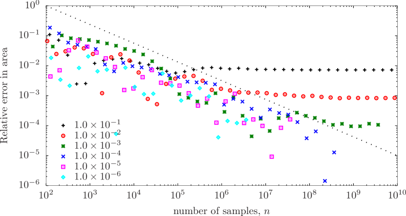
Figure 1: Relative error in the estimate for the area of an isosurface in the simple example with $\psi=4$.

The term “relative error” is not strictly correct because the method arrives at the correct areas based on layers of finite thickness. For this simple case, the area of the surface with $\phi=\psi+\Delta\phi$ will always be larger than the area of the isosurface $\phi=\psi$. For example, the relative difference between the analytically determined areas of the surfaces with $\psi=4$ and $4.01$ is approximately $0.001$, which is consistent with figure 1. Importantly, though, the area estimate converges linearly with $\Delta\phi$ as expected from the derivation of (6). This is apparent from the figure because, for the three layer thicknesses for which the evaluation of (6) is converged, the area estimate improves by an order of magnitude as $\Delta\phi$ is decreased by an order of magnitude.

We conclude from this simple case that the method can be used to measure isosurface areas with arbitrary accuracy given a sufficiently small $\Delta\phi$ and sufficient samples. The area converges with $n^{-1/2}$ and with $\Delta\phi$. One caveat is that care must be used in accumulating the statistics, such as by using 128-bit floating point arithmetic and, perhaps, the method of Kahan (1965) to reduce roundoff errors; both techniques are used in this paper. A second caveat is that pseudo-random sequences have limitations which are beyond the scope here but are discussed in, e.g., Vadhan et al. (2012). Also, it is interesting to note that the quantity ${V(\psi,\Delta\phi)}/(V\ \Delta\phi)$ is in fact a first order approximation to $P(\phi;\phi=\psi)$ provided that the Monte Carlo integration is converged. Further discussion of this is in appendix A.

4 Direct Numerical Simulations

The simulated flows are the solution to the Navier-Stokes equations and passive scalar transport equation in three spatial dimensions:

$$\nabla\cdot\vec{u}=0$$ (8a)

$${{\partial\vec{u}}\over{\partial t}}+\vec{u}\cdot\nabla\vec{u}=-\nabla p+\nu\nabla^{2}\vec{u}+\vec{b}$$ (8b)

$$\frac{\partial\phi}{\partial t}+\vec{u}\cdot\nabla\phi=-\vec{u}\cdot\nabla\Phi+D\nabla^{2}\phi\ .$$ (8c)

The velocity vector is $\vec{u}=[u,v,w]$ with kinematic viscosity $\nu$, the pressure $p$ has been divided through by the (constant) density, and $\vec{b}$ is a time-varying force applied to maintain the flow statistically stationary. The passive scalar is decomposed into $\Phi+\phi$, with time-invariant $\Phi$ having a uniform gradient in the direction of $w$, and being uniform in the other spatial directions; $\phi$ denotes the fluctuations relative to $\Phi$ with molecular diffusivity $D$.

Spatial discretisation is via Fourier series truncated according to the 2/3 rule to remove all effects of aliasing. The advection terms are computed in real space in vorticity form for momentum and in convective and conservation forms on alternating time steps for the scalars. The equations are advanced in time using a third order accurate fractional step method for the advection and pressure gradient terms while the diffusion terms are integrated exactly in Fourier space.

The velocity fields are forced isotropically so that the three-dimensional kinetic energy spectrum at length scales larger than the integral length scale matches Pope’s model spectrum with his $p_{0}=2$ and his $c_{L}=6.78$ (Pope, 2000, (equation 6.247)). Each time step, a second-order ordinary differential equation is advanced in time for each shell of the shell-averaged spectrum to determine how much energy to add to that shell. The energy is distributed randomly, but consistent with continuity, across all the wave numbers composing the shell. The solution to these differential equations and the random distributions produces the Fourier-space equivalent of $\vec{b}$. This approach is introduced by Overholt & Pope (1998) to efficiently converge a simulation to a target spectrum; Rao & de Bruyn Kops (2011) reviews a variety of forcing techniques for the type of simulation used for this research. After the simulation was determined to be statistically stationary based on mean quantities, it was advanced for an additional large eddy turnover time before taking a snapshot for analysis of the isosurface areas.

Seven velocity fields are considered for this research, with each convecting four scalar fields with differing Schmidt numbers $\mathit{Sc}=\nu/D$. The velocity field statistics are tabulated in table 1 and the scalar statistics in table 2

	R24	R42	R98	R154	R245	R400	R633
$\mathit{Re_{L}}$	49.8	114	310	734	1853	4790	12150
$\mathit{Re_{\lambda}}$	24.0	42.3	97.8	154	245	400	633
${\cal L}/L$	5.5	6.7	5.2	5.7	5.7	5.6	5.6
$\kappa_{max}L_{k}$	9.73	9.14	26.84	12.90	6.48	9.39	5.65
$L_{k}/\Delta$	4.66	4.38	12.82	6.16	6.64	4.48	2.70
$\tau_{k}/\Delta t$	90	103	1376	1165	954	1170	1202
$N$	512	1024	4096	4096	8800	11760	14256
Reference			R1	R2	R3	R4

Table 1: Velocity parameters and statistics for the highest resolution of each case. $N$ and $\kappa_{max}L_{k}$ are shown for each velocity field at it highest resolution ($\mathit{Sc}=7$); lower resolution is used for the cases with lower $\mathit{Sc}$ in simulations R245, R400, and R633 and the resolution for each scalar case is given in table 2 in terms of $L_{k}/\Delta$. ‘Reference’ indicates the names used for statistically equivalent simulations in Almalkie & de Bruyn Kops (2012a), de Bruyn Kops (2015), Muschinski & de Bruyn Kops (2015) and Portwood et al. (2016).

$Pe_{\lambda}$	$Sc$	$L_{k}/\Delta x$	$L_{c}/\Delta x$	$L_{b}/\Delta x$	$\tau_{k}/\Delta t$	$\tau_{c}/\Delta t$	$Re_{\lambda}$
2.40	0.10	4.66	26.23	14.75	89.95	284.43	24
4.23	0.10	4.38	24.63	13.85	103.09	326.01	42
9.78	0.10	12.82	72.08	40.53	1376.14	4351.74	98
15.37	0.10	6.16	34.64	19.48	1164.67	3683.00	154
16.82	0.70	4.66	6.09	5.57	89.95	107.51	24
24.03	1.00	4.66	4.66	4.66	89.95	89.95	24
24.46	0.10	4.53	25.48	14.33	953.77	3016.08	245
29.58	0.70	4.38	5.72	5.23	103.09	123.22	42
40.01	0.10	2.22	12.51	7.03	485.56	1535.47	400
42.25	1.00	4.38	4.38	4.38	103.09	103.09	42
63.27	0.10	1.55	8.71	4.90	779.68	2465.55	633
68.47	0.70	12.82	16.75	15.32	1376.14	1644.80	98
97.81	1.00	12.82	12.82	12.82	1376.14	1376.14	98
107.59	0.70	6.16	8.05	7.36	1164.67	1392.04	154
153.70	1.00	6.16	6.16	6.16	1164.67	1164.67	154
168.24	7.00	4.66	1.08	1.76	89.95	34.00	24
171.22	0.70	4.53	5.92	5.41	953.77	1139.97	245
244.60	1.00	4.53	4.53	4.53	953.77	953.77	245
280.05	0.70	2.22	2.91	2.66	485.56	580.35	400
295.76	7.00	4.38	1.02	1.66	103.09	38.97	42
400.07	1.00	2.22	2.22	2.22	485.56	485.56	400
442.86	0.70	1.55	2.02	1.85	779.68	931.89	633
632.65	1.00	1.55	1.55	1.55	779.68	779.68	633
684.65	7.00	12.82	2.98	4.84	1376.14	520.13	98
1075.87	7.00	6.16	1.43	2.33	1164.67	440.20	154
1712.20	7.00	6.64	1.54	2.51	953.77	360.49	245
2800.48	7.00	4.48	1.04	1.70	1170.48	442.40	400
4428.57	7.00	2.70	0.63	1.02	1202.44	454.48	633

Table 2: Scalar field parameters and statistics all cases.

with $\mathit{Re_{L}}$ the Reynolds number based on the r.m.s. velocity and the integral length scale $L$, $\mathit{Re_{\lambda}}$ the Reynolds number based on the r.m.s. velocity and the Taylor microscale and $\mathit{Pe_{\lambda}}$ the corresponding Péclet number. $L_{k}$, $L_{b}$, and $L_{c}$ are the Kolmogorov, Batchelor, and Oboukhov-Corrsin length scales, respectively,

$$L_{k}=\left(\frac{\nu^{3}}{\epsilon}\right)^{1/4},\ \ \ L_{b}=\left(\frac{\nu D^{2}}{\epsilon}\right)^{1/4},\ \ \ L_{c}=\left(\frac{D^{3}}{\epsilon}\right)^{1/4}$$ (9)

with corresponding times scales

$$\tau_{k}=\frac{\nu}{\epsilon}^{1/2},\ \ \ \tau_{c}=\frac{D}{\epsilon}^{1/2}\ .$$ (10)

Here $\epsilon$ is the dissipation rate of kinetic energy. The maximum wave number after dealiasing is $\kappa_{max}$, the grid spacing is $\Delta x$, and the time step size is $\Delta t$. The domain size is $\cal L$ in each spatial direction discretised by $N$ grid points.

The velocity fields are denoted by an R followed by $\mathit{Re_{\lambda}}$ rounded to an integer, e.g. R24. Four of the cases have been reported elsewhere so that cases R98, R154, and R245 are statistically equivalent to cases R1, R2, and R3 reported by Almalkie & de Bruyn Kops (2012a) and R400 is equivalent to the homogeneous isotropic case denoted R4 in Almalkie & de Bruyn Kops (2012b), de Bruyn Kops (2015) and Portwood et al. (2016). The R400 is denoted R4 by Muschinski & de Bruyn Kops (2015) and used to study models for scalar energy spectra.

5 Numerical considerations

Before proceeding to evaluating isosurface areas in the DNS as a function of Reynolds and Schmidt numbers in §6, it is important to apply the tests from §3 to understand the accuracy to which the areas can be evaluated from the DNS. It is also important to understand the extent to which the spatial and temporal resolution of the DNS may effect the area calculations. These are the topics of this section. We do not review the numerical errors in Fourier spectral methods because they are discussed so extensively in the literature and instead refer the reader to, e.g., de Bruyn Kops & Riley (2001, §3).

Fourier spectral simulations represent the scalar fields as infinite series with all but a few of the series coefficients identically zero. This is in contrast to, say, a laboratory time series which has been Fourier transformed and represented by a truncated series. This characteristic of the current simulations allows us to sample the scalar fields at an arbitrary number of locations via phase shifting so that each sample has the same accuracy as the simulation as a whole and no interpolation error is introduced. Also in Fourier spectral simulations, $\nabla\phi$ is known with the same accuracy as $\phi$ because the derivative of each term in the series expansion is known analytically.

The sampling process begins with the scalar field in Fourier space. A random phase shift with wave number vector $\vec{\kappa}$ is applied, the field is transformed to real space, and all of the points in the resulting field are used to accumulate data for evaluating (6). The process is repeated as many times as desired. The result is a Monte Carlo method in which for every $N^{3}$ samples of the field only one random vector $\kappa$ is chosen. Because the samples for a single value $\vec{\kappa}$ are uniformly distributed across the entire simulation domain, this method is a type of “quasi-random” sampling (c.f. §3).

The spatial and temporal resolution requirements in DNS have been continually refined over the last three decades as computers have gotten more powerful so as to enable simulations with higher internal intermittency. The large-scale requirement for decaying homogeneous isotropic turbulence (HIT) was established by experimentation to be about 20 times the integral length scale $L$ by de Bruyn Kops & Riley (1998b) and recently verified by de Bruyn Kops & Riley (2019). In simulations forced to be statistically stationary, such as those used for the current research, no large-scale resolution requirement has been established to our knowledge, and we have used domains that are approximately $5L$ because this resolution has been shown to produce structure functions and spectra that match theoretical predictions in the inertial and dissipation ranges (Almalkie & de Bruyn Kops, 2012a).

Small scale resolution requirements for DNS were first established by Eswaran & Pope (1988), who showed that $\kappa_{max}L_{k}>1$ is required for the scalar variance to decay as expected from theory in decaying HIT. Since then, the dependency of small scale statistics on Reynolds number has been analysed in several studies (Yeung & Sawford, 2002; Yeung et al., 2005; Ishihara et al., 2007; Gulitski et al., 2007b, a; Ishihara et al., 2009) and the effects on intermittency of insufficient small-scale resolution in DNS investigated (Yakhot & Sreenivasan, 2005; Schumacher et al., 2007; Watanabe & Gotoh, 2007; Donzis et al., 2008). Recently, Yeung et al. (2018) report on not only the spatial resolution required to resolve small-scale intermittency but also the temporal resolution for $\mathit{Re_{\lambda}}=390$ and 650, which are comparable to our cases R400 and R633. Because of our need to resolve $\mathit{Sc}=7$, our spatial resolutions are finer than those shown to be sufficient in the paper just referenced. Therefore, when we satisfy the Courant number condition established by Yeung et al. our timestep is smaller than theirs, which gives us confidence that the time scale of intermittency is resolved. The time step in each simulation is given in table 1, relative to the Corrsin and Kolmogorov time scales, from which it is apparent that these time scales are very well resolved in the simulations.

The foregoing gives us confidence that all the scalar and velocity fields are well resolved and so we move to the question of the effect of layer thickness $\Delta\phi$ used in numerically evaluating (6). For the simple example illustrated by figure 1, the error in an isosurface area reduces unbounded and proportionally to $n^{-1/2}$ and $\Delta\phi$. Recall that the exact area in that case is known. In the DNS fields, though, the exact area is not known so that the error in the area must be based on the best available area estimate, e.g., that computed with the scalar field at the highest resolution available and with the smallest practicable layer thickness. Also, we can surmise that, even with careful attention to mitigating them with 128-bit arithmetic and the method of Kahan (1965), roundoff errors will limit the accuracy of the numerical evaluation of (6).

Our test case for numerical studies is R245 because the Reynolds number is high enough for there to be significant intermittency yet we have resolved it with much finer spatial resolution than required per Yeung et al. (2018). $\Pr=7$ is considered since it has the smallest diffusive length scale. The relative errors for the area of a single isosurface $\psi$ computed using various layer thicknesses is shown as figure 2. The dimensionless layer thickness is

$$\widetilde{\Delta\phi}=\frac{\Delta\phi}{L_{r}\left<|\nabla\phi|\right>_{\bm{X}_{\psi}}}$$ (11)

with $L_{r}$ being some resolution length scale appropriate for the scalar. In this paper we set $L_{r}=\Delta x$ because, in our simulations, $\Delta x<L_{b}$ for $Pr\geq 1$ and $\Delta x\leq L_{c}$ for $Pr\leq 1$.

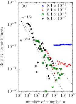
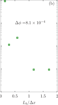
Figure 2: Error in the area of one isosurface in case R245, $Pr=7$, for various nondimensional layer thicknesses $\widetilde{\Delta\phi}$ (panel (a)) and grid resolutions (panel (b)). The dotted lines labelled $n^{-1/2}$ and $n^{-2/3}$ mark the convergence rates expected for pseudo-random and quasi-random sampling, respectively (Press et al., 2007).

The first thing to note from the figure 2(a) is that the leftmost symbol in each set is the number of samples $n$ in a layer of thickness $\widetilde{\Delta\phi}$ before phase shifting, e.g., when $\widehat{\Delta\phi}=8.1\times 10^{-5}$ approximately $10^{5}$ points are in $[\phi,\psi+\Delta\phi)$. Next it is noted that when $\widetilde{\Delta\phi}=8.1\times 10^{-2}$, the minimum relative error is approximately $10^{-3}$ and does not decrease with more sampling. For smaller $\widetilde{\Delta\phi}$, the isosurface area estimates converge at a rate between $n^{-1/2}$, which is expected for pseudo-random sequences, and $n^{-2/3}$, which is expected for quasi-random sequences. Our sampling method is based on phase shifting the entire field based on a randomly selected $\kappa$ so that the sampling for a single phase shift is quasi-random but the phase shifts are pseudo-random.

Given enough samples for a given $\Delta\phi$ the area estimate converges just as it does in §3. For example, when $\widetilde{\Delta\phi}=8.1\times 10^{-3}$ then the minimum relative error is approximately $1\times 10^{-4}$ meaning that the isosurface area estimate converges to a value different from the “exact” value taken to be the estimate when $\widetilde{\Delta\phi}=8.1\times 10^{-5}$. As explained in §3, the term “relative error” is not quite correct because the method computes the area based on a layer of finite thickness so that the area based on $\widetilde{\Delta\phi}=8.1\times 10^{-3}$ is expected to be different from that based on $\widetilde{\Delta\phi}=8.1\times 10^{-5}$ even if both areas are computed exactly.

From figure 2(a) we conclude that the error in the area estimate can be made arbitrarily small given a small enough layer thickness and a sufficient number of samples produced by phase shifting. This conclusion is conditioned on the assumption that the simulations are sufficiently resolved at the small scale. We have already concluded that we expect them to be, based on the requirements determined by Yeung et al. (2018), but we verify it one more time with figure 2(b). The “exact” area for this plot is from a simulation with $L_{b}/\Delta x=2.5$ that is filtered with a spectral cutoff filter to produce the fields with lower values of $L_{b}/\Delta$ used to make the figure. It is observed that the error in the area estimate converges to its minimum value when $L_{b}/\Delta x=1$. Note from figure 2(a) that this minimum value of approximately $1\times 10^{-4}$ is set by the layer thickness, not the resolution of the simulation.

6 Effects of $\bm{\mathit{Re_{\lambda}}}$ and $\bm{Sc}$ on isosurfaces

The time rate of change of the area of a non-material isosurface is determined by the balance between stretching tangential to the surface and diffusion normal to the surface. A detailed derivation is included in Dopazo et al. (2018) for the case of a chemically reacting flow. For our purpose here we follow their notation and consider an infinitesimal piece of an isosurface having area $\cal S$ with normal vector $n_{i}$ and strain rate $S_{ij}$ so that the strain rate tangential to the surface is $a_{T}=(\delta_{ij}-n_{i}n_{j})S_{ij}$. A point on an isosurface moves by diffusion, relative to the speed at which the surface is advected, with speed $S_{d}=-D\nabla^{2}\phi/\nabla\phi$. Therefore the fractional change in area of this piece of an isosurface is (c.f. Dopazo et al., 2018, equation 25)

$$\frac{1}{\cal S}\frac{\partial\cal S}{\partial t}=a_{T}+S_{d}\frac{\partial n_{i}}{\partial x_{i}}\ .$$ (12)

For the statistically stationary flows, the integral of (12) over an entire isosurface is zero meaning that the integrals of two terms on the right hand side of (12) come into equilibrium.

The central physics question motivating this paper is how the equilibrium surface area $A_{\psi}$ is affected by Reynolds and Schmidt number. Catrakis et al. (2002) measured area-volume properties of fluid interfaces in a laboratory water jet with jet Reynolds number $\sim 20,000$ and $Sc\sim 2000$ and report that, while large and small length scales contribute to the area-volume ratio, the dominant effect is at the small scales. They conclude that self-similarity at the small scales can be expected to enable extrapolation of area-volume behaviour to higher Reynolds number. Schumacher & Sreenivasan (2005) consider DNS of a passive scalar with a mean gradient in homogeneous isotropic turbulence with $10\leq\mathit{Re_{\lambda}}\leq 42$ and $2\leq Sc\leq 32$ and observe that the area-volume ratio increases with both $Sc$ and $\mathit{Re_{\lambda}}$ but that a power law is not observed. They further note that power law behaviour is not expected because, at the Reynolds and Schmidt numbers considered, neither the inertial-convective nor the viscous-convective subranges exist. O’Neill & Soria (2005) also consider DNS of homogeneous isotropic turbulence with a mean scalar gradient with $Sc=0.25$ and 5.0 and $\mathit{Re_{\lambda}}=41$, 42, and 77. They observe that increasing either $\mathit{Re_{\lambda}}$ or $Sc$ results in the size of the isoscalar surfaces decreasing. We note that they determine the areas with a geometric method and review in §1 some of the challenges with using geometric methods to find the areas of turbulent isosurfaces.

In the literature just cited, the metric for isosurface area is the area-volume ratio. Our simulations are computed in periodic domains, however, so that the scalar can be convected out of the domain to a periodic domain above or below. Given this configuration, we find it to be more clear to take advantage of homogeneity in the flows and consider the dimensionless ratio of the wrinkled surface to the initial surface area, which is that of a plane normal to the mean scalar gradient. The wrinkled surface area includes that of any portions of the surface advected across the periodic boundaries. To be precise, we compute the volume of a very thin wrinkled layer with $\widetilde{\Delta\phi}=1\times 10^{-4}$ and relate it to an isosurface area via (6). The results are in figure 3.

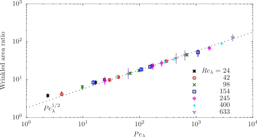
Figure 3: Isosurface areas normalised by the area of a horizontal plane in the simulations. The symbols mark the average for 20 isovalues and the bars indicate the range from the largest to smallest areas. The dotted line is a reference line, not a fitted line.

For each case, the areas are measured for 20 iso-values spanning the range of $\phi$ in the simulation. It is noted that there is more scatter in some cases than in others, and this appears to be due to limited large-scale resolution so that large structures occur which are resolved in space but not resolved statistically. In appendix B, we demonstrate for several simulation cases that the scatter in the areas is much smaller simulation domain is eight times larger.

The provisional conclusion drawn from figure 3 is that the area increases with $Pe_{\lambda}^{1/2}$ for $Pe_{\lambda}^{1/2}>50$ and may deviate from power law scaling for $Pe_{\lambda}^{1/2}<50$. The second part of this conclusion is influenced by the finding by Schumacher & Sreenivasan (2005) that the area increases with Péclet number but with no power law scaling; they consider flows with lower $\mathit{Re_{\lambda}}$ than all but our cases R24 and R48. We consider this conclusion in more detail in the remainder of this section, but we immediately note that it is not in agreement with the results of O’Neill & Soria (2005) who report a decrease in area with increasing Reynolds and Schmidt number. Their result, however, is based on visual geometric methods, the limitations of which we discuss in §1. Our results are in broad agreement with the conclusion of Catrakis et al. (2002) that small-scale similarity is expected; note that the current flow configuration does not allow us to compare with their results regarding variations in large-scale features of the flow, but we do consider the effects of large scale resolution in appendix B and show that the average isosurface area does not change with domain size but the scatter in the areas of different isosurfaces in a simulation decreases as the domain size increases and the large-scale statistics improve.

Our range of $\mathit{Pe_{\lambda}}$ overlaps that of Schumacher & Sreenivasan (2005), but, except for our cases R24 and R42, our Reynolds numbers are much higher. So now let us consider our conclusions from the previous paragraph in more detail and, in particular, the point made by Schumacher & Sreenivasan (2005) that they do not expect to see fractal-like behaviour of an isosurfaces because of the absence of inertial-convective and the viscous-convective subranges. Definitive identification of these subranges in a simulation is difficult because of noisy statistics in the spectra and structure functions and the presence of the so-called spectral blocking “bump” at the top of the dissipation range; Ishihara et al. (2009, 2016) provide reviews. We can say with confidence that we do not expect an inertial subrange in our cases R24, R42, and R98 but that subranges do exist in cases R245, R400, and R633. This is based not only on detailed analysis of our data (Almalkie & de Bruyn Kops, 2012a; de Bruyn Kops, 2015) but also of simulations by Yeung et al. (2005) and the two papers just cited by Ishihara et al. Yeung et al. show very clear inertial subranges for $\mathit{Re_{\lambda}}\geq 240$, which corresponds to our cases R245, R400, and R633. Given the robust literature on the existence of inertial ranges as a function of $\mathit{Re_{\lambda}}$, we do not show the inertial range analyses for all of our data sets here. We do so next for our case with the highest Péclet number because it has not been previously published.

The compensated shell-averaged spectra of kinetic and scalar energies for the case with $\mathit{Pe_{\lambda}}=4429$ are shown in figure 4

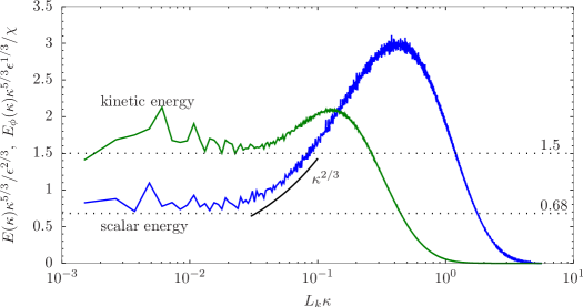
Figure 4: Spherical shell-averaged spectra of kinetic and scalar energies for the case with $\mathit{Pe_{\lambda}}=4429$. The dotted lines indicated the expected levels for the inertial-convective range discussed in the text. The solid like marked $\kappa^{2/3}$ is the ’slope’ of the compensated Batchelor spectrum, not a fitted curve.

with $E(\kappa)$ and $E_{\phi}(\kappa)$ the kinetic and scalar energy spectra, respectively, $\epsilon$ the domain-averaged dissipation rate of kinetic energy, and $\chi$ the corresponding value for scalar variance. The textbook value for the Kolmogorov constant of $C=1.5$ (Pope, 2000) is indicated by a horizontal dotted line on the figure. The Oboukhov-Corrsin constant $C_{\phi}=0.68$ is determined by Muschinski & de Bruyn Kops (2015) for a simulation very similar to the current cases with $\mathit{Pe_{\lambda}}=280$ and 400 and is consistent with values determined by Sreenivasan & Kailasnath (1996) and Watanabe & Gotoh (2004); it is also marked by a horizontal dotted line on the figure. We conclude that the inertial-convective subrange spans about a decade in wave number based on the range over which the plateaus in both spectra corresponds with the appropriate dotted line. The span of of the subrange is consistent with the results of Yeung et al. (2005) for their case with $\mathit{Re_{\lambda}}=700$.

The viscous-convective subrange is not as easy to identify because of the so-called “Hill bump” that includes this subrange and continues into the dissipation range (Hill, 1978). The viscous-convective range, if it exists, is expected to begin at about $L_{k}\kappa=0.03$ (Muschinski & de Bruyn Kops, 2015). If the viscous-convective subrange exists then we expect to see the compensated scalar spectrum scaling with $\kappa^{2/3}$ and this scaling is marked on the figure with a solid line labelled accordingly. It appears that the scalar spectrum exhibits this scaling over a fraction of a decade of wave numbers in the viscous-convective subrange. Of course the spectrum necessarily transitions from the plateau to the Hill bump in the dissipation range and so it is difficult to clearly identify a narrow viscous-convective subrange, which is why we do not present this analysis for the cases with lower $\mathit{Pe_{\lambda}}$.

Next, let us consider the probability density functions of the local scalar gradient on an isosurface plotted as figure 5 for five layers in each case.

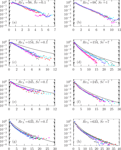
Figure 5: Probability density of the local gradient magnitudes on a layer normalised by the mean for that layer. The horizontal axis is $|\nabla\phi|_{V(\psi,\Delta\phi)}/\langle|\nabla\phi|\rangle_{V(\psi,\Delta\phi)}$. Five layers are shown for each case with their nominal locations distributed uniformly over the vertical extent of the domain in this order of lowest to highest $\phi$: plus, circle, cross, square, diamond. In panels (c) though (h), the solid line marks the standard log-normal distribution.

In panels (a) and (b) the distributions are very close to exponential, consistent with the results of Schumacher & Sreenivasan (2005). In panels (e), (f), (g), and (h) they tend toward lognormal with the lognormal distribution being a very good model for some of the layers in panel (h). In panels (c) and (d), it is difficult to draw a conclusion although in our opinion the curves are neither straight enough to be consider exponential nor is the lognormal distribution a good model. Note that the change in the distribution from exponential to one closer to lognormal is appears primarily to be due to increased $\mathit{Re_{\lambda}}$ largely independent of either $\mathit{Pe_{\lambda}}$ or $Sc$. This suggests that the exponential distribution occurs when there is no inertial-convective subrange. Recall that case R98 has no inertial subrange whereas our cases R245, R400, and R633 have characteristics of inertial subranges.

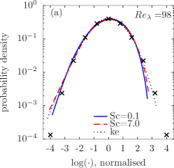
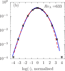
Figure 6: P.d.f.s of the logarithm of the dissipation rates for the variances of scalars with $Sc=0.1$ and 7.0 and for kinetic energy, all normalised by their means and variances. The crosses mark the standard Gaussian.

Significant scatter is observed figure 5 among the distributions for the five layers in each set. The governing equations we solve numerically describe a homogeneous flow but in a simulation domain of finite size the homogeneity is not perfect. In appendix B we conclude that the areas of different isosurfaces converge to a common value as the domain size increases. So the effects of limited domain size observed in the scatter in figure 5 are interesting in itself. It is most clear in panel (d) in which the lowest curve is approximately exponential while the upper curve is approximately lognormal. Recall from the literature reviewed in this section that an inertial-convective range is expected for $\mathit{Re_{\lambda}}>240$ but not necessarily at $\mathit{Re_{\lambda}}=154$, which is the value for panels (c) and (d). The result is consistent with $\mathit{Re_{\lambda}}>154$ being between $\mathit{Re_{\lambda}}=98$, for which an inertial-convective range is not expected, and $\mathit{Re_{\lambda}}=245$ for which one is expected.

A different view of the same data is presented in figure 6. More precisely, the p.d.f.s are shown for the natural logarithm of the local dissipation rate of scalar variance $\chi_{0}=2D\nabla\phi\cdot\nabla\phi$ using data for the whole domain. By plotting this quantity, comparisons can be made with the logarithm of the p.d.f. of the local dissipation rate of kinetic energy $\epsilon_{0}$. For $\mathit{Re_{\lambda}}=98$, $\epsilon_{0}$ has an approximately lognormal distribution, except for very small values of $\epsilon_{0}$, whereas the scalar does not. For both cases shown with $\mathit{Re_{\lambda}}=98$ and for $\mathit{Re_{\lambda}}=633$ with $Sc=0.1$ we observe that the p.d.f. for high values of $\chi_{0}$ lies inside that of $\epsilon_{0}$. This behaviour was first noted, to our knowledge, in laboratory measurements in boundary layers (Antonia & Sreenivasan, 1977) and later in in DNS of homogeneous isotropic turbulence (e.g. Vedula et al., 2001). For $\mathit{Re_{\lambda}}=633$ and $Sc=7.0$, however, this behaviour occurs only at the very highest values of $\chi_{0}$. This suggests that, if the Péclet number were high enough then the lognormal model would be a good approximation for $\chi_{0}$, except for very small values at which the p.d.f.s of $\chi_{0}$ and $\epsilon_{0}$ depart from lognormality but agree with each other.

7 Conclusions

The area of a scalar isosurface can be written exactly in terms of the limit of the volume of a thin layer as the layer thickness goes to zero, which is shown in the development of (6). Numerically evaluating (6) to arbitrarily small relative error in DNS via a Monte-Carlo method requires being able to evaluate accurately the scalar field at arbitrary locations, which can be done in the case of pseudospectral simulations. We demonstrate the evaluation of the surface areas for an analytical test case and then with DNS data and observe the expected convergence behaviours as the thickness of the layer is reduced and the number of samples increases. For the DNS, it is observed that with sufficient spatial resolution of the simulation and a sufficiently thin layer width that the relative error in the area of an isosurface can be reduced to $1\times 10^{-4}$ or smaller. In the process of determining this, we verify the small-scale resolution criterion recently provided by Yeung et al. (2018).

Next the methodology is applied to 28 DNS cases of statistically stationary homogeneous isotropic turbulence with a mean scalar gradient, $0.1\leq Sc\leq 7$ and $24.0\leq\mathit{Re_{\lambda}}\leq 633$. It is observed that the layer area is very nearly proportional to $\mathit{Pe_{\lambda}}^{1/2}$ over the range $50\leq\mathit{Pe_{\lambda}}\leq 4429$ and may depart from this scaling when $\mathit{Pe_{\lambda}}<50$. This result is broadly consistent with the literature although direct comparisons are not possible because other studies used geometric estimates for isosurface areas rather than direct calculations.

To understand the results better, we expand on analysis by Schumacher & Sreenivasan (2005) and examine the p.d.f.s of the scalar gradient on multiple layers in each simulation and observe that at low $\mathit{Re_{\lambda}}$ they are modelled very well by an exponential distribution. For our highest $\mathit{Re_{\lambda}}$ case, the lognormal distribution is a much better model, and we also see convincing evidence of the existence of a viscous-convective subrange in this case. Indeed, for $\mathit{Re_{\lambda}}=633$ and $Sc=7.0$, the lognormal model is very good for the p.d.f. of the scalar dissipation rate, and the difference between the p.d.f. of the scalar and kinetic energy dissipation rates is extremely small. These results, combined with those of Schumacher & Sreenivasan (2005) suggest that the isosurface area scales with $\mathit{Pe_{\lambda}}^{1/2}$ only if there is an inertial-convective subrange but does not require there to be a viscous-convective subrange. The new results also suggest that the difference between the p.d.f.s of the scalar and kinetic energy dissipation rates, which has long been observed, might occur only when the Reynolds number is not sufficiently high.

Appendix A Relationship between $\bm{A(\psi)/V}$ and $\bm{P(\phi;\phi=\psi)}$

At the end of §3 we note that the the ratio ${V(\psi,\Delta\phi)}/(V\ \Delta\phi)$ is an approximation to $P(\phi;\phi=\psi)$. We show here our rationale for that statement and also present an analysis for the order of accuracy of (6). Recall from §2 that $A(\psi)$ denotes the exact area of the surface with $\phi=\psi$. The ratio ${V(\psi,\Delta\phi)}/{V}$ is the ratio of the number of locations with scalar value between $\psi$ and $\psi+\Delta\phi$ to the total number of locations, which equals the probability $p(\phi;\psi\leq\phi<\psi+\Delta\phi)$ of finding a point with scalar value in the range $[\phi,\phi+\Delta\phi)$. This equivalence of ${V(\psi,\Delta\phi)}/{V}$ with the probability of finding a position $\vec{x}$ such that $\phi(\vec{x})\in[\psi,\psi+\Delta\phi)$ follows from $\vec{x}$ being a uniformly distributed random variable. If $P(\phi)$ is the p.d.f. of $\phi$ then, from the definition of a p.d.f.,

$$\frac{V(\psi,\Delta\phi)}{V}=p(\phi;\psi\leq\phi+\Delta\phi)=\int_{\psi}^{\psi+\Delta\phi}P(\phi)d\phi\ .$$ (13)

Using the rectangle rule, the left hand side in (4) can be written

$$\int_{\psi}^{\psi+\Delta\phi}A(\phi)d\phi={A(\psi)\Delta\phi}+k_{A}(\Delta\phi){\Delta\phi}^{2}\ ,$$ (14)

where $k_{A}(\Delta\phi)$ denotes the maximum value of ${dA(\phi)}{d\phi}$ in the domain $[\psi,\psi+\Delta\phi)$. Using (4), (13) and (14), we arrive at

$$\frac{{A(\psi)\Delta\phi}+k_{A}(\Delta\phi){\Delta\phi}^{2}}{V}={\int_{\psi}^{\psi+\Delta\phi}P(\phi)d\phi}\ {\langle|\nabla\phi|\rangle_{V(\psi,\Delta\phi)}}\ .$$ (15)

Dividing through by $\Delta\phi$ yields

$$\frac{A(\psi)}{V}=\frac{\int_{\psi}^{\psi+\Delta\phi}P(\phi)d\phi}{\Delta\phi}\ {\langle|\nabla\phi|\rangle_{V(\psi,\Delta\phi)}}-\frac{k_{A}(\Delta\phi)}{V}{\Delta\phi}\ ,$$ (16)

which is a first order approximation for the area to volume ratio. Finally, approximating the integral of the p.d.f. with the rectangle rule results in

$$\frac{A(\psi)}{V}=\frac{P(\phi;\phi=\psi)\Delta\phi+k_{p}(\Delta\phi){\Delta\phi}^{2}}{\Delta\phi}\ {\langle|\nabla\phi|\rangle_{V(\psi,\Delta\phi)}}-\frac{k_{A}(\Delta\phi)}{V}{\Delta\phi}\ ,$$ (17)

where $k_{P}(\Delta\phi)$ is the maximum value of ${dP(\phi)}{d\phi}$ in the domain $[\psi,\psi+\Delta\phi)$. By comparing (17) and (6) we see that, if the Monte-Carlo integration of the latter is converged, then it provides a first-order approximation of $P(\phi;\phi=\psi)$. The integral in 14 can also be evaluated with a higher order approximation. Shete (2019, Chapter 5, Figure 5.10) evaluates the integral using the midpoint rule, which is a second order method, and obtain second order convergence with layer thickness. The definition of $P(\phi)$ in the turbulence literature, e.g., (Pope, 2000), is as the limit of a histogram with bins extending from $\phi$ to $\phi+\Delta\phi$. To strictly preserve the relationships discussed in this appendix we have used first-order integration to evaluate isosurface areas in this paper.

Appendix B Effect of Large Scales

Equation (3) shows that an isosurface area is a function of $\nabla\phi$ and Catrakis et al. (2002) conclude that while large and small length scales in a jet contribute to the area-volume ratio, the dominant effect is at the small scales. Therefore, we do not expect the area calculations to be strongly affected by domain size. Also, in conjunction with figure 3 we assert that, while the equations and boundary conditions describe a homogeneous flow, the simulations are not perfectly homogeneous because the domain size is finite so that different isosurfaces have slightly different areas; the error bars in figure 3 indicate the extent to which the statistics of the large scales are not resolved in each simulation. In principle the large-scale statistics can be improved by aggregating them over time, but it is impractical to advance large simulations for sufficiently long times and doing so would not improve the statistics for a single snapshot of the flow. Therefore, in this appendix, we examine the effects on our conclusions of the large scales and their statistical convergence in single snapshots in time.

We compare here the isosurface areas for pairs of equivalent simulations. The first simulation in each pair is that used for the main body this paper and denoted either R24 or R42. The second simulation in each pair is statistically the same but resolved in a domain eight times larger in each dimension. The small-scale resolution for both variants of R24 is the same while for R42 the grid spacing in the large domain is twice that in the small domain. The ratio of the domain size to the integral length scale ${\cal L}/L$ is approximately 45 for the large domain size, which is significantly larger than the value of 20 reported by de Bruyn Kops & Riley (1998a) as being necessary for decaying HIT to have sufficiently large-scale resolution to decay at the same rate as grid turbulence in a wind tunnel.

The results from this test are tabulated in table 3 for the scalar fields with the highest and lowest Schmidt numbers. In each case, the mean surface area for the large domain is within the range of areas for the small domain, and the difference between the minimum and maximum areas is smaller for the larger domain. We conclude that the surface areas are insensitive to the size of the domain and that the areas of all isosurfaces approach the same value as the domain size increases.

				R24				R42
Domain		Sc		mean	min	max		mean	min	max
Small		0.1		3.82	3.32	4.32		4.16	3.84	5.00
Large		0.1		3.91	3.89	3.93		4.25	4.20	4.40
Small		7.0		23.58	20.68	25.58		30.84	28.68	33.14
Large		7.0		24.17	23.88	24.42		30.91	30.54	31.15

Table 3: The mean, minimum, and maximum isosurface areas in equivalent simulations run in differing domain sizes. All areas are per unit volume times the volume of the smaller domain.

References

- Almalkie & de Bruyn Kops (2012a) Almalkie, S. & de Bruyn Kops, S. M. 2012a Energy dissipation rate surrogates in incompressible Navier-Stokes turbulence. J. Fluid Mech. 697, 204–236.
- Almalkie & de Bruyn Kops (2012b) Almalkie, S. & de Bruyn Kops, S. M. 2012b Kinetic energy dynamics in forced, homogeneous, and axisymmetric stably stratified turbulence. J. Turbul. 13 (29), 1–29.
- Antonia & Sreenivasan (1977) Antonia, R. A. & Sreenivasan, K. R. 1977 Lognormality of temperature dissipation in a turbulent boundary layer. Phys. Fluids 20 (11), 1800–1804.
- Bohr (2007) Bohr, M. 2007 A 30 year retrospective on dennard’s mosfet scaling paper. IEEE Solid-State Circuits Society Newsletter 12 (1), 11–13.
- Bray (2016) Bray, K. 2016 Laminar flamelets in turbulent combustion modeling. Combustion Science and Technology 188 (9), 1372–1375.
- Bray & Swaminathan (2006) Bray, K. N. & Swaminathan, N. 2006 Scalar dissipation and flame surface density in premixed turbulent combustion. Comptes Rendus - Mecanique 334 (8-9), 466–473.
- de Bruyn Kops (2015) de Bruyn Kops, S. M. 2015 Classical turbulence scaling and intermittency in stably stratified Boussinesq turbulence. J. Fluid Mech. 775, 436–463.
- de Bruyn Kops & Riley (1998a) de Bruyn Kops, S. M. & Riley, J. J. 1998a Direct numerical simulation of laboratory experiments in isotropic turbulence. Phys. Fluids 10 (9), 2125–2127.
- de Bruyn Kops & Riley (1998b) de Bruyn Kops, S. M. & Riley, J. J. 1998b Scalar transport characteristics of the linear-eddy model. Combust. Flame 112 (1/2), 253–260.
- de Bruyn Kops & Riley (2001) de Bruyn Kops, S. M. & Riley, J. J. 2001 Mixing models for large-eddy simulation of non-premixed turbulent combustion. J. Fluids. Eng. 123 (2), 341–346.
- de Bruyn Kops & Riley (2019) de Bruyn Kops, S. M. & Riley, J. J. 2019 The effects of stable stratification on the decay of initially isotropic homogeneous turbulence. J. Fluid Mech. 860, 787–821.
- Catrakis et al. (2002) Catrakis, H. J., Aguirre, R. C. & Ruiz-Plancarte, J. 2002 Area-volume properties of fluid interfaces in turbulence: Scale-local self-similarity and cumulative scale dependence. Journal of Fluid Mechanics 462, 245–254.
- Chaudhuri et al. (2017) Chaudhuri, S., Kolla, H., Dave, H. L., Hawkes, E. R., Chen, J. H. & Law, C. K. 2017 Flame thickness and conditional scalar dissipation rate in a premixed temporal turbulent reacting jet. Combustion and Flame .
- Corrsin & Kistler (1955) Corrsin, S. & Kistler, A. L. 1955 Free-stream boundaries of turbulent flows. NACA Report 1224, 1033–1064.
- Delichatsios (1987) Delichatsios, M. A. 1987 Air entrainment into buoyant jet flames and pool fires. Combustion and Flame 70 (1), 33–46.
- Dennard et al. (1974) Dennard, R. H., Gaensslen, F. H., Rideout, V. L., Bassous, E. & LeBlanc, A. R. 1974 Design of ion-implanted mosfet’s with very small physical dimensions. IEEE Journal of Solid-State Circuits 9 (5), 256–268.
- Dimov et al. (2007) Dimov, I. T., Penzov, A. A. & Stoilova, S. S. 2007 Parallel monte carlo approach for integration of the rendering equation. In Numerical Methods and Applications (ed. T. Boyanov, S. Dimova, K. Georgiev & G. Nikolov), pp. 140–147. Berlin, Heidelberg: Springer Berlin Heidelberg.
- Donzis et al. (2008) Donzis, D. A., Yeung, P. K. & Sreenivasan, K. R. 2008 Dissipation and enstrophy in isotropic turbulence: Resolution effects and scaling in direct numerical simulations. Phys. Fluids 20 (4), 045108.
- Dopazo et al. (2018) Dopazo, C., Martin, J., Cifuentes, L. & Hierro, J. 2018 Strain, Rotation and Curvature of Non-material Propagating Iso-scalar Surfaces in Homogeneous Turbulence. Flow Turbul. Combust. 101 (1), 1–32.
- Eswaran & Pope (1988) Eswaran, V. & Pope, S. B. 1988 Direct numerical simulations of the turbulent mixing of a passive scalar. Phys. Fluids 31, 506–520.
- Federer (1959) Federer, H. 1959 Curvature measures. Transactions of the American Mathematical Society 93 (3), 418–491.
- Freedman & Diaconis (1981) Freedman, D. & Diaconis, P. 1981 On the histogram as a density estimator:l2 theory. Z. Wahrscheinlichkeit. 57 (4), 453–476.
- Gulitski et al. (2007a) Gulitski, G., Kholmyansky, M., Kinzelbach, W., Lüthi, B., Tsinober, A. & Yorish, S. 2007a Velocity and temperature derivatives in high-Reynolds-number turbulent flows in the atmospheric surface layer. Part 2. Accelerations and related matters. J. Fluid Mech. 589, 83–102.
- Gulitski et al. (2007b) Gulitski, G., Kholmyansky, M., Kinzelbach, W., Lüthi, B., Tsinober, A. & Yorish, S. 2007b Velocity and temperature derivatives in high-Reynolds-number turbulent flows in the atmospheric surface layer. Part 3. Temperature and joint statistics of temperature and velocity derivatives. J. Fluid Mech. 589, 103–123.
- Hill (1978) Hill, R. J. 1978 Models of the scalar spectrum for turbulent advection. J. Fluid Mech. 88 (3), 541–562.
- Ishihara et al. (2009) Ishihara, T., Gotoh, T. & Kaneda, Y. 2009 Study of high-Reynolds number isotropic turbulence by direct numerical simulation. Annu. Rev. Fluid Mech. 41, 165–180.
- Ishihara et al. (2007) Ishihara, T., Kaneda, Y., Yokokawa, M., Itakura, K. & Uno, A. 2007 Small-scale statistics in high-resolution direct numerical simulation of turbulence: Reynolds number dependence of one-point velocity gradient statistics. J. Fluid Mech. 592, 335–366.
- Ishihara et al. (2016) Ishihara, T., Morishita, K., Yokokawa, M., Uno, A. & Kaneda, Y. 2016 Energy spectrum in high-resolution direct numerical simulations of turbulence. Phys. Rev. Fluids 1, 082403.
- Kahan (1965) Kahan, W. 1965 Pracniques: further remarks on reducing truncation errors. Commun. ACM 8 (1), 40.
- Kim & Bilger (2007) Kim, S. Y. & Bilger, R. W. 2007 Iso-surface mass flow density and its implications for turbulent mixing and combustion. J. Fluid Mech. 590, 381–409.
- Kolla & Chen (2018) Kolla, H. & Chen, J. H. 2018 Turbulent Combustion Simulations with High-Performance Computing, pp. 73–97. Singapore: Springer Singapore.
- Lewiner et al. (2003) Lewiner, T., Lopes, H., Vieira, A. W. & Tavares, G. 2003 Efficient implementation of marching cubes’ cases with topological guarantees. J. Graph. Tools 8 (2), 1–15.
- Liu et al. (2010) Liu, Y. S., Yi, J., Zhang, H., Zheng, G. Q. & Paul, J. C. 2010 Surface area estimation of digitized 3D objects using quasi-Monte Carlo methods. Pattern Recognition .
- Muschinski & de Bruyn Kops (2015) Muschinski, A. & de Bruyn Kops, S. M. 2015 Investigation of Hill’s optical turbulence model by means of direct numerical simulation. J. Opt. Soc. Am. A 32 (12), 2423–2430.
- Newman & Yi (2006) Newman, T. S. & Yi, H. 2006 A survey of the marching cubes algorithm. Comput. Graph. 30 (5), 854 – 879.
- O’Neill & Soria (2005) O’Neill, P. L. & Soria, J. 2005 The topology of homogeneous isotropic turbulence with passive scalar transport. In Proc. of 12th Computational Techniques and Applications Conference, CTAC-2004 (ed. R. May & A. J. Roberts), ANZIAM J., vol. 46, pp. C1170–C1187.
- Overholt & Pope (1998) Overholt, M. R. & Pope, S. B. 1998 A deterministic forcing scheme for direct numerical simulations of turbulence. Comput. Fluids 27, 11–28.
- Patera & Skala (2004) Patera, J. & Skala, V. 2004 A comparison of fundamental methods for iso surface extraction. Machine Graphics and Vision 13 (4), 329–343.
- Payne et al. (1988) Payne, J. L., Hassan, B. & Af I, . S. 1988 Massively Parallel Computational Fluid Dynamics Calculations for Aerodynamics and Aerothermodynamics Applications. Tech. Rep..
- Peters (2000) Peters, N. 2000 Turbulent combustion. Cambridge university press.
- Pope (1988) Pope, S. 1988 The evolution of surfaces in turbulence. Int. J. Eng. Sci. 26 (5), 445 – 469.
- Pope (2000) Pope, S. B. 2000 Turbulent Flows. Cambridge: Cambridge University Press.
- Pope et al. (1989) Pope, S. B., Yeung, P. K. & Girimaji, S. S. 1989 The curvature of material surfaces in isotropic turbulence. Phys. Fluids A-Fluid 1 (12), 2010–2018.
- Portwood et al. (2016) Portwood, G. D., de Bruyn Kops, S. M., Taylor, J. R., Salehipour, H. & Caulfield, C. P. 2016 Robust identification of dynamically distinct regions in stratified turbulence. J. Fluid Mech. 807, R2 (14 pages).
- Press et al. (2007) Press, W. H., Teukolsky, S. A., Vetterling, W. T. & Flannery, B. P. 2007 Numerical Recipes 3rd Edition: The Art of Scientific Computing, 3rd edn. New York, NY, USA: Cambridge University Press.
- Raase & Nordström (2015) Raase, S. & Nordström, T. 2015 On the use of a many-core processor for computational fluid dynamics simulations. In Procedia Comput. Sci..
- Rao & de Bruyn Kops (2011) Rao, K. J. & de Bruyn Kops, S. M. 2011 A mathematical framework for forcing turbulence applied to horizontally homogeneous stratified flow. Phys. Fluids 23, 065110.
- Resnikoff & Raymond Jr (2012) Resnikoff, H. L. & Raymond Jr, O. 2012 Wavelet analysis: the scalable structure of information. New York: Springer Science & Business Media.
- Ricou & Spalding (1961) Ricou, F. P. & Spalding, D. B. 1961 Measurements of entrainment by axisymmetrical turbulent jets. J. Fluid Mech. 11 (1), 21–32.
- Scheidegger et al. (2008) Scheidegger, C. E., Schreiner, J. M., Duffy, B., Carr, H. & Silva, C. T. 2008 Revisiting histograms and isosurface statistics. IEEE T. Vis. Comput. Gr. 14 (6), 1659–1666.
- Schroeder et al. (2006) Schroeder, W., Martin, K., Lorensen, B., Avila, L. S., Avila, R. & Law, C. C. 2006 The Visualization Toolkit An Object-Oriented Approach To 3D Graphics Fourth Edition. Tech. Rep..
- Schumacher & Sreenivasan (2005) Schumacher, J. & Sreenivasan, K. R. 2005 Statistics and geometry of passive scalars in turbulence. Phys. Fluids .
- Schumacher et al. (2007) Schumacher, J., Sreenivasan, K. R. & Yakhot, V. 2007 Asymptotic exponents from low-Reynolds-number flows. New J. Phys. 9, 89.
- Shete (2019) Shete, K. P. 2019 Calculation of isosurface areas and applications. Master’s thesis, University of Massachusetts Amherst.
- Sobol’ (1967) Sobol’, I. M. 1967 On the distribution of points in a cube and the approximate evaluation of integrals. Zhurnal Vychislitel’noi Matematiki i Matematicheskoi Fiziki 7 (4), 784–802.
- Sreenivasan & Kailasnath (1996) Sreenivasan, K. R. & Kailasnath, P. 1996 The passive scalar spectrum and the Obukhov-Corrsin constant. Phys. Fluids 8, 189–96.
- Swaminathan & Bray (2011) Swaminathan, N. & Bray, K. 2011 Turbulent Premixed Flames. Cambridge University Press.
- Taveira & da Silva (2014) Taveira, R. R. & da Silva, C. B. 2014 Characteristics of the viscous superlayer in shear free turbulence and in planar turbulent jets. Phys. Fluids 26 (2), 021702.
- Vadhan et al. (2012) Vadhan, S. P. et al. 2012 Pseudorandomness. Foundations and Trends in Theoretical Computer Science 7 (1–3), 1–336.
- Vedula et al. (2001) Vedula, P., Yeung, P. K. & Fox, R. O. 2001 Dynamics of scalar dissipation in isotropic turbulence: a numerical and modelling study. J. Fluid Mech. 433, 29–60.
- Watanabe & Gotoh (2004) Watanabe, T. & Gotoh, T. 2004 Statistics of a passive scalar in homogeneous turbulence. New J. Phys. 6 (40), 1–36.
- Watanabe & Gotoh (2007) Watanabe, T. & Gotoh, T. 2007 Inertial-range intermittency and accuracy of direct numerical simulation for turbulence and passive scalar turbulence. J. Fluid Mech. 590, 117–146.
- Watanabe et al. (2016) Watanabe, T., Riley, J. J., de Bruyn Kops, S. M., Diamessis, P. J. & Zhou, Q. 2016 Turbulent/non-turbulent interfaces in wakes in stably stratified fluids. J. Fluid Mech. 797, R1.
- Yakhot & Sreenivasan (2005) Yakhot, V. & Sreenivasan, K. R. 2005 Anomalous scaling of structure functions and dynamic constraints on turbulence simulations. J. Stat. Phys. 121, 823–841.
- Yeung et al. (2018) Yeung, P., Sreenivasan, K. & Pope, S. 2018 Effects of finite spatial and temporal resolution in direct numerical simulations of incompressible isotropic turbulence. Phys. Rev. Fluids 3 (6), 064603.
- Yeung et al. (2005) Yeung, P. K., Donzis, D. A. & Sreenivasan, K. R. 2005 High-Reynolds-number simulation of turbulent mixing. Phys. Fluids 17, 081703.
- Yeung & Sawford (2002) Yeung, P. K. & Sawford, B. L. 2002 Random-sweeping hypothesis for passive scalars in isotropic turbulence. J. Fluid Mech. 459, 129–138.
- Yurtoglu et al. (2018) Yurtoglu, M., Carton, M. & Storti, D. 2018 Treat all integrals as volume integrals: A unified, parallel, grid-based method for evaluation of volume, surface, and path integrals on implicitly defined domains. J. Inf. Sci. Eng. 18 (2), 021013.
- Zheng et al. (2017) Zheng, T., You, J. & Yang, Y. 2017 Principal curvatures and area ratio of propagating surfaces in isotropic turbulence. Phys. Rev. Fluids 2, 103201.