Boosting High Dimensional Predictive Regressions with Time Varying Parameters

Abstract

High dimensional predictive regressions are useful in wide range of applications. However, the theory is mainly developed assuming that the model is stationary with time invariant parameters. This is at odds with the prevalent evidence for parameter instability in economic time series, but theories for parameter instability are mainly developed for models with a small number of covariates. In this paper, we present two $L_{2}$ boosting algorithms for estimating high dimensional models in which the coefficients are modeled as functions evolving smoothly over time and the predictors are locally stationary. The first method uses componentwise local constant estimators as base learner, while the second relies on componentwise local linear estimators. We establish consistency of both methods, and address the practical issues of choosing the bandwidth for the base learners and the number of boosting iterations. In an extensive application to macroeconomic forecasting with many potential predictors, we find that the benefits to modeling time variation are substantial and they increase with the forecast horizon. Furthermore, the timing of the benefits suggests that the Great Moderation is associated with substantial instability in the conditional mean of various economic series.

Keywords: $L_{2}$ Boosting, Forecasting, Locally Stationary, Parameter Instability, Sparsity.

JEL Classification: C1, C2.

1 Introduction

Due to the rapid improvements in the information technology, high dimensional time series datasets are frequently encountered in a variety of fields in economics and finance (see Fan et al. (2011); Shapiro (2017) for examples). In these settings, the number of candidate predictors ($p_{T}$) is much larger than the number of samples ($T$), and accurate estimation and prediction is made possible by relying on some form of dimension reduction. Ng (2013) puts the methods used in high dimension predictive regressions into two classes: a dense class which assumes that the covariates have a low rank representation that can be exploited for subsequent modeling, and a sparse class which assumes that the number of relevant predictors is far smaller than the number of predictors available. Research within the first class usually assumes a linear latent factor model which is estimated by principal components or partial least squares. The second class treats the problem as one of variable selection in high dimension. Prominent methods in this class include screening, penalized likelihood, lasso, and boosting methods.

This paper contributes to the literature in the second class. A key assumption made in the vast majority of works on sparse modeling is of a stationary underlying model with time invariant parameters. The assumption is very restrictive in practice, as empirical evidence of parameter instability and time varying effects have been well documented in macroeconomics. Parameter instability can be driven by structural changes in technological advancements, government or monetary policy changes, and preference shifts at the individual level (Chen and Hong, 2012). Ignoring these instabilities can lead to large forecasting errors, with Clements and Hendry (1996) and others even arguing that these instabilities are the main source of error for forecasting models.

Consider a high dimensional linear time varying parameter (TVP) model:

$$Y_{t}=\bm{\beta}_{t}\bm{x}_{t-h}+\epsilon_{t}\textrm{ for }t=1,\ldots,T,$$ (1)

where $Y_{t}$ is the response, $\bm{x}_{t-h}=(X_{1,t-h},\ldots,X_{p_{T},t-h})$ is a $p_{T}$-dimensional vector of predictors (with $p_{T}>>T$), $\bm{\beta}=(\beta_{1,t},\ldots,\beta_{p_{T},t})$ is a vector of time varying parameters, and $\epsilon_{t}$ are errors; the precise assumptions on the model will be stated in section 3. Given the evidence for parameter instability, the question remains on how to best represent and model this change, especially when dealing with high dimensional predictors. Parameter instability is most commonly represented in the econometrics literature by random walks or by one or more discrete structural breaks. Modeling variations by random walks can be quite restrictive as it imposes a specific structure on the evolution of the parameters. Discrete breaks require knowledge of the break dates, and not all time variations are well characterized by discrete shifts. Technology and taste shifts are arguably evolving slowly over time. Smooth transition models as in Terasvirta (1994) are still tightly parameterized. Furthemore, these methods are mainly designed for a fixed $p_{T}$. A third approach is to use rolling-window estimation to capture the smooth change in the parameters. As will soon be clear, rolling-window estimation is a special case of our proposed approach with a particular choice of kernel and bandwidth.

In this paper, we model these high-dimensional parameters as smooth functions of time whose functional forms are unknown and are estimated non-parametrically. We present two $L_{2}$ boosting algorithms which differ in their choice of base learners; the first uses componentwise local constant estimators as base learners, while the second relies on componentwise local linear estimators as base learners. We consider the use of local linear estimators since they have been shown to be a superior estimator theoretically, with smaller asymptotic bias at the boundaries of the sample (Cai, 2007). We establish consistency of both our methods when dealing with high dimensional locally stationary predictors and errors with only polynomially decaying tails. Although we focus on linear time varying parameter models, $L_{2}$ boosting methods can easily be adapted to fit more general non-linear models by considering alternative base learners such as regression trees with varying degrees of depth. This makes the $L_{2}$ boosting framework more flexible than the often used $\ell_{1}$ penalized likelihood approaches.

The smooth TVP model considered in this paper has been studied in the econometrics literature for the case when the number of predictors is fixed and assumed known. Under this assumption, Robinson (1989, 1991) studied the asymptotic properties of the local constant estimator of the coefficient functions. The theory was further developed in several directions. To our knowledge, there were only two attempts at modeling sparse high dimensional smooth TVP models, both dealing with locally stationary sub-Gaussian predictors, and rely on $l_{1}$ regularization methods along with kernel smoothing to estimate the coefficient functions. In particular, Ding et al. (2017) deals with locally stationary sparse VAR processes, and proposes a hybrid estimator which combines $l_{1}$ regularization with local constant estimation. Lee et al. (2016) deals with models where the set of non-zero coefficient functions does not change with over time, and proposes a computationally intensive penalized local linear estimation method. Our work adds to this line of research by proposing $L_{2}$ boosting algorithms for high dimensional smooth TVP models characterized by (1).

Our methods compare favorably to more commonly used alternatives for modeling time varying parameters such as assuming the coefficients are stochastic and generated by a random walk, or using a rolling window estimator with a fixed window length. These models are typically estimated via MCMC, or other computationally intensive methods, which excludes the use of high dimensional datasets. Rolling window forecasts, although they are usually not presented this way, are actually equivalent to using a local constant estimator using a uniform kernel and a fixed bandwidth. This choice of fixed bandwidth is arbitrary and can lead to larger forecast errors vs using the optimal bandwidth (Inoue et al., 2017). Additionally, local constant estimators have higher asymptotic bias at the boundary of the sample vs local linear estimators. In contrast, our $L_{2}$ boosting algorithms are capable of variable selection and estimation simultaneously at a very low computational cost even for very high dimensional data. Also, using non-parametric methods to estimate the time varying coefficient functions allows our method to perform well even under model misspecifications such as discrete breaks, stochastic coefficients generated by a random walk, and time invariant coefficients; see Giraitis et al. (2013); Inoue et al. (2017) and our simulations section for more details.

On the empirical side we include an extensive application to macroeconomic forecasting. Although parameter instability has long been established in the econometrics literature (Stock and Watson, 2003, 2009; Breitung and Eickmeier, 2011), the question of whether one can exploit this instability to improve macroeconomic forecasts is far less clear (see section 7 or Rossi (2013) for more details). Some issues which have hindered the utility of modeling time variation are: 1) the bias-variance tradeoff encountered when using a reduced sample for modeling, 2) misspecification and/or estimation error incurred when trying to estimate the nature of time variation, and 3) computational constraints restricting the use of high dimensional predictors when estimating traditional TVP models with stochastic coefficients.

To analyze the effectiveness of modeling time variation with our methods, we use a panel of 123 monthly series from the FRED-MD database and focus on forecasting 8 major macroeconomic series over a range of forecast horizons. Using an out of sample period of over 47 years, we find that: 1) the benefits of modeling time variation with our methods are substantial, especially when considering longer forecast horizons, 2) the timing of these benefits suggests that the Great Moderation is associated with large amounts of parameter instability in the conditional mean of various economic series, and 3) the benefits of modeling time variation appear to be confined to the high dimensional setting, as we confirm the results in Stock and Watson (1996) that modeling time variation in AR models offers little to no benefits for the majority of series.

The rest of the paper is organized as follows. Section 2 reviews the locally stationary framework, along with the functional dependence measure which will be used to quantify dependence. We also discuss the assumptions placed on the structure of the covariate and response processes; these assumptions are very mild, allowing us to represent a wide variety of stochastic processes which arise in practice. Section 3 introduces our boosting algorithms for both local constant or local linear least squares base learners, and studies the asymptotic properties of these procedures. The asymptotic properties, and the number of predictors allowed depend on the strength of dependence, and the moment conditions of the underlying processes. Section 6 presents results from Monte Carlo simulations, and sections 7 and 8 contain our application to macroeconomic forecasting. Lastly, concluding remarks are in section 9.

2 The Econometric Framework

We first start with a review of locally stationary processes which were first introduced by Dahlhaus (1996); Dahlhaus et al. (1997) using a time varying spectral representation. This was expanded in Dahlhaus et al. (2018) to a more general definition which facilitated theoretical results for a large class of non-linear processes; see Dahlhaus (2012) for a partial survey of the results pertaining to locally stationary processes. Heuristically speaking, a locally stationary process is a non-stationary process which can be well approximated by a stationary process locally in time. This is a convenient framework to model non-stationarity induced by smooth time varying parameters. Consider the model (1), with $\bm{\beta}_{t}$ being a vector of unknown deterministic smooth functions of time, as a consequence $Y_{t}$ in (1) is clearly non-stationary. Due to this non-stationarity, letting $T\rightarrow\infty$ will not lead to consistent estimates of $\bm{\beta}_{t}$, since future observations may not contain any information about the probabilistic structure of the process at the present time $t$. Therefore, it is common to work in the infill asymptotics framework with rescaled time $t/T\in[0,1]$, with $\bm{\beta}_{t}=\bm{\beta}(t/T)$ (Dahlhaus et al., 1997; Robinson, 1989; Cai, 2007). Letting $T\rightarrow\infty$ now implies that we observe $\bm{\beta}(t/T)$ on a finer grid within the same interval, thereby increasing the amount of local information available. Although this setting is not commonly seen in forecasting time series, a prediction theory is still possible. For example, we can view our data as having been observed for $t=1,\ldots,T/2$ (i.e. on the interval $[0,1/2]$), and we are forecasting the next few observations (see Dahlhaus et al. (1997); Dahlhaus (1996)).

For a formal description of locally stationary processes we use the definition and assumptions stated in Dahlhaus et al. (2018) and Richter and Dahlhaus (2018):

Definition 2.1.

Let $q>0$, and $||W||_{q}=(E|W|^{q})^{1/q}$. Let $Y_{t,T},t=1,\ldots,T$ be a triangular array of stochastic processes. For each $u\in[0,1]$, let $\tilde{Y}_{t}(u)$ be a stationary and ergodic process satisfying:

1. $D_{q}=\max\{\sup_{u\in[0,1]}||\tilde{Y}_{t}(u)||_{q},\sup_{T\in N}\sup_{t=1,\ldots,T}||Y_{t,T}||_{q}\}<\infty$

2. There exists $C_{B}>0$ such that uniformly in $t=1,\ldots,T$ and $u,v\in[0,1]$:

   $$||\tilde{Y}_{t}(u)-\tilde{Y}_{t}(v)||_{q}\leq C_{B}|u-v|,\textrm{ }||Y_{t,T}-\tilde{Y}_{t}(t/T)||_{q}\leq C_{B}T^{-1}$$ (2)

From the second assumption we obtain: $||Y_{t,T}-\tilde{Y}_{t}(u)||_{q}\leq O(|t/T-u|+T^{-1})$, thus for rescaled time points $t/T$ near $u$, the process $Y_{t,T}$ can be approximated by a stationary process $\tilde{Y}_{t}(u)$ with asymptotically negligible error. Consider the model used in Robinson (1989); Cai (2007): $Y_{t,T}=\bm{\beta}(t/T)\bm{X}_{t}+\epsilon_{t}$, where $\bm{X}_{t},\epsilon_{t}$ are stationary processes, and $\bm{\beta}(\cdot)$ is a lipschitz continuous function. Under these conditions $Y_{t,T}$ is a locally stationary process, with stationary approximation: $\tilde{Y}_{t}(u)=\bm{\beta}(u)\bm{X}_{t}+\epsilon_{t}$. A slightly more complicated example is a tvAR(1) process: $Y_{t,T}=\alpha(t/T)Y_{t-1,T}+\epsilon_{t}=\sum_{j=0}^{\infty}[\prod_{k=1}^{j-1}\alpha(\frac{t-k}{T})]\epsilon_{t-j}$. Intuitively one can see that if we assume $\alpha(\cdot)$ is lipschitz continuous then the process is locally stationary with stationary approximation: $\tilde{Y}_{t}(u)=\alpha(u)\tilde{Y}_{t-1}(u)+\epsilon_{t}$, and $||Y_{t,T}-\tilde{Y}_{t}(u)||_{q}\leq O(|t/T-u|+T^{-1})$. The stationary approximation is the key to estimation and formulating an asymptotic theory when dealing with locally stationary processes. Estimation of parameters such as $\alpha(u)$ and local covariances is carried out by assuming, for each rescaled time point $u$, that the process is essentially stationary on a small window around $u$. We then carry out estimation via stationary methods using observations within this window.

In order to establish asymptotic properties of our $L_{2}$ boosting procedures, we rely on the functional dependence measure introduced in Wu (2005) and used in the context of locally stationary processes in Dahlhaus et al. (2018); Richter and Dahlhaus (2018). We first introduce the following notation: Let $\{e_{t}\}_{t\in\mathcal{Z}}$ be a sequence of iid random variables, and let $\mathcal{F}_{t}=(e_{t},e_{t-1},\ldots)$, $\mathcal{F}_{t}^{*}=(e_{t},e_{t-1},\ldots,e_{0}^{*},e_{-1},\ldots)$ with $e_{0}^{*},e_{t},t\in\mathbb{Z}$ being iid. Additionally, let $\mathcal{H}_{t}=(\bm{\eta}_{t},\bm{\eta}_{t-1},\ldots)$, $\mathcal{H}_{t}^{*}=(\bm{\eta}_{t},\bm{\eta}_{t-1},\ldots,\bm{\eta}_{0}^{*},\bm{\eta}_{-1},\ldots)$ with $\bm{\eta}_{0}^{*},\bm{\eta}_{t},t\in\mathbb{Z}$ being iid random vectors. Throughout this paper, we assume the following structure for the stationary approximation for univariate processes (such as the response and error processes), and multivariate processes (such as the covariate process) respectively:

$$\tilde{Y}_{t}(u)=g(u,\mathcal{F}_{t})\textrm{ and }\bm{\tilde{x}}_{t}(u)=\bm{h}(u,\mathcal{H}_{t})=(h_{1}(u,\mathcal{H}_{t}),\ldots,h_{p_{T}}(u,\mathcal{H}_{t})),$$ (3)

where $g(\cdot,\cdot)$, and $\bm{h}(\cdot,\cdot)$ are real valued measurable functions. These representations allow us to define the functional dependence measure as: $\delta_{q}^{\tilde{Y}(u)}(t)=||\tilde{Y}_{t}(u)-g(u,\mathcal{F}_{t}^{*})||_{q}$, and $\delta_{q}^{\tilde{X}_{j}(u)}(t)=||\tilde{X}_{j,t}(u)-h_{j}(u,\mathcal{H}_{t}^{*})||_{q}$. Additionally, we assume short range dependence of the form:

$$\Delta_{0,q}^{\tilde{Y}}=\sum_{k=0}^{\infty}\sup_{u\in[0,1]}\delta_{q}^{\tilde{Y}(u)}(k)\leq\infty,\textrm{ and }\Phi_{0,q}^{\bm{\tilde{x}}}=\max_{j\leq p_{T}}\sum_{k=0}^{\infty}\sup_{u\in[0,1]}\delta_{q}^{\tilde{X}_{j}(u)}(k)\leq\infty,$$ (4)

for some $q>2$ to be specified in the next section.

We place assumptions on the stationary approximation rather than directly on the process itself. This leads to results using weaker assumptions, and to more interpretable dependence measures. For an intuitive explanation of this measure, we consider the stationary approximation at time $u_{0}$ ($\tilde{Y}_{t}(u_{0})$) and we obtain $\delta_{q}^{\tilde{Y}(u_{0})}(k)=||\tilde{Y}_{k}(u_{0})-g(u_{0},\mathcal{F}_{k}^{*})||_{q}$. We can view $\delta_{q}^{\tilde{Y}(u_{0})}(k)$ as measuring the dependence of $\tilde{Y}_{k}(u_{0})$ on the innovation $\epsilon_{0}$, which for weakly dependent processes decreases suitably quickly as $k\rightarrow\infty$. For a concrete example, consider a stationary AR(1) process $\tilde{Y}_{t}(u_{0})=\sum_{j=0}^{\infty}a(u_{0})^{j}e_{t-j}$ with $e_{i}$ iid, then $\delta_{q}^{\tilde{Y}(u_{0})}(k)=|a(u_{0})^{k}|||e_{0}-e_{0}^{*}||_{q}$, and $\Delta_{0,q}^{\tilde{Y}(u_{0})}=||e_{0}-e_{0}^{*}||_{q}\sum_{k=0}^{\infty}|a(u_{0})^{k}|$. Now in the locally stationary setting, we take the supremum over the rescaled time interval to account for the non-stationarity of the processes, thereby obtaining $\Delta_{0,q}^{\tilde{Y}}=||e_{0}-e_{0}^{*}||_{q}\sup_{u\in[0,1]}\sum_{k=0}^{\infty}|a(u)^{k}|$. A very wide variety of locally stationary processes encountered in practice including time varying linear processes, tv-ARMA, tv-GARCH, tv-TAR, and tv-VAR, and time varying random coefficient processes have stationary approximations which satisfy (4), and have geometrically decaying functional dependence measures (see Dahlhaus et al. (2018)).

Compared to mixing coefficients, functional dependence measures are easier to interpret and compute since they are directly related to the data generating mechanism of the underlying process. For example, consider a stationary ARMA($p,q$) process, $\xi_{t}=e_{t}+\sum_{i=1}^{p}\alpha_{i}\xi_{t-i}+\sum_{j=1}^{q}\beta_{j}e_{t-j}$ with $e_{t}$ iid, under appropriate conditions we can show this process is $\beta$-mixing with $\beta(t)=O(\rho^{t})$ and $\rho\in(0,1)$ (Doukhan, 1994). However, there exists no known mapping between the parameters and $\rho$ (McDonald et al., 2015). In contrast, by using the moving average representation for $\xi_{t}=\sum_{j=0}^{\infty}f_{j}e_{i-j}$, we see the functional dependence measure is directly related to the data generating process: $\delta_{q}(\xi_{t})=O(f_{t})$. Additionally, in many cases using functional dependence measures also requires less stringent assumptions (Yousuf, 2018; Wu, 2005). We do note that functional dependence measures are restricted to a more limited class of processes, specifically those possessing the representation (3). Fortunately, this is a very weak restriction as virtually all time series models used in practice have this representation (see Hörmann et al. (2010); Wu (2011) and references therein).

3 Boosting High Dimensional TVP Models

Ever since the introduction of AdaBoost in the 1990’s (Freund and Schapire, 1997), boosting algorithms have been one of the most successful and widely utilized machine learning methods (Friedman et al., 2001). AdaBoost, which was developed for classification, consisted of iteratively fitting a series of weak classifiers or learners onto reweighted data and taking a weighted average of the predictions from each of these simple models. The success of AdaBoost was originally thought to originate from averaging many weak classifiers and from a reweighting scheme which placed large weights on heavily misclassified observations. Later work by Friedman (2001), and Friedman et al. (2000) established AdaBoost as a gradient descent algorithm in function space using an exponential loss function. This functional gradient descent view connected boosting to the common optimization view of statistical inference, and led to extensions of boosting beyond the realm of classification. Friedman (2001) proposed several new boosting algorithms using alternative base learners and loss functions including squared error loss, leading to $L_{2}$ boosting. Additionally, Efron et al. (2004) and Friedman et al. (2001), made connections for linear models between $L_{2}$ boosting and common statistical procedures such as the Lasso and forward stagewise regression. These insights shed light on $L_{2}$ boosting as a method which performs variable selection and shrinkage leading to sparse models. For an excellent survey of the statistical view of boosting and results pertaining to several common boosting algorithms, one can consult Buhlmann and Hothorn (2007).

We are interested in estimating the following model:

$$Y_{t,T}=\bm{\beta}^{\prime}(t/T)\bm{x}_{t-h,T}+\epsilon_{t,T}\textrm{ for }t=1,\ldots,T,$$ (5)

where $Y_{t,T}$ is the response, $\bm{x}_{t-h,T}=(X_{1,t-h,T},\ldots,X_{p_{T},t-h,T})^{\prime}$ is a $p_{T}$-dimensional vector of locally stationary predictors (with $p_{T}>>T$), $\bm{\beta}^{\prime}(t/T)=(\beta_{1}(t/T),\ldots,\beta_{p_{T}}(t/T))$ is a vector of unknown functions of time defined on the grid $[0,1]$, which becomes finer as $T\rightarrow\infty$, and $\epsilon_{t,T}$ denotes the locally stationary error process with $E(\epsilon_{t,T}\bm{x}_{t-h,T})=0\textrm{ }\forall\textrm{ }t,T$. We denote the stationary approximation of the response as $\tilde{Y}_{t}(u)=\bm{\beta}^{\prime}(u)\tilde{\bm{x}}_{t-h}(u)+\tilde{\epsilon}_{t}(u)$. To simplify notation, we discuss estimation at the boundary point $u=T/T=1$. Before we introduce our boosting algorithms, it helps to first introduce the population version of componentwise $L_{2}$ boosting with linear base learners as applied to the stationary approximations $(\tilde{Y}_{T}(u),\tilde{\bm{x}}_{T-h}(u))$:

Algorithm: Population level $L_{2}$ Boosting

1. Set $F^{(0)}(u,\tilde{\bm{x}}_{T-h}(u))=E(\tilde{Y}_{T}(u))$

2. For $m=1,\ldots,M_{T}$, where $M_{T}$ is some stopping iteration, do:

   1. Compute $\tilde{U}^{(m)}_{T}(u)=\tilde{Y}_{T}(u)-F^{(m-1)}(u,\tilde{\bm{x}}_{T-h}(u))$.

   2. Let $\mathcal{S}_{m}=\mbox{argmin}_{j\leq p_{T}}E(\tilde{U}_{T}^{(m)}(u)-\alpha_{j}^{(m)}(u)\tilde{X}_{j,T-h}(u))^{2}$,
      where $\alpha^{(m)}_{j}(u)=E(\tilde{X}_{j,T-h}(u)\tilde{U}_{T}^{(m)}(u))/E(\tilde{X}^{2}_{j,T-h}(u))$.

   3. Update $F^{(m)}(u,\tilde{\bm{x}}_{T-h}(u))=F^{(m-1)}(u,\tilde{\bm{x}}_{T-h}(u))+\upsilon\cdot\alpha^{(m)}_{\mathcal{S}_{m}}(u)\tilde{X}_{\mathcal{S}_{m},T-h}(u)$, where $\upsilon\in(0,1]$ is a step length factor.

3. Output ${F}^{(M_{T})}(u,\tilde{\bm{x}}_{T-h}(u))=F^{(0)}(u,\tilde{\bm{x}}_{T-h}(u))+\upsilon\sum_{m=1}^{M_{T}}\alpha^{(m)}_{\mathcal{S}_{m}}(u)\tilde{X}_{\mathcal{S}_{m},T-h}(u)$

Although we use linear base learners, we note that our methods can be extended to a broader class of models by using a more general base learner, such as $g_{j}(u,\tilde{X}_{j,T-h}(u))=E(\tilde{Y}_{T}(u)|\tilde{X}_{j,T-h}(u))$, and estimating using kernel regressions or smoothing splines. For the corresponding sample version of $L_{2}$ boosting with linear base learners, it is informative to consider the case of stationary response and predictor processes. In the stationary setting, we can remove the dependence on $T$ and the sample version of our algorithm simplifies to $\mathcal{\hat{S}}_{m}=\mbox{argmin}_{j}\sum_{t=1}^{T}(U^{(m)}_{t}-\hat{\alpha}^{(m)}_{j}X_{t,j})^{2}$, where $\hat{\alpha}^{(m)}_{j}=T^{-1}\sum_{t=1}^{T}X_{j,t-h}U^{(m)}_{t}$, assuming $E(X_{t}),E(Y_{t})=0$, and $E(X_{t}^{2})=1$. For the case of locally stationary response and predictor processes the situation is more complicated as the above estimator is inconsistent for $\alpha_{j}^{(m)}(u)$. Intuitively, this inconsistency arises since observations “far” from rescaled time $u$ contain little information about the probabilistic structure of the processes at time $u$.

To proceed with estimation in the locally stationary setting, $\forall m$ and $j\leq p_{T}$, we have $U^{(m)}_{t,T}=\alpha^{(m)}_{j}(t/T)X_{j,t-h,T}+\epsilon_{j,t,T}$, where $\alpha^{(m)}_{j}(t/T)=E(\tilde{X}_{j,t-h}(t/T)\tilde{U}^{(m)}_{T}(t/T))/E(\tilde{X}^{2}_{j,t-h}(t/T))$. By local stationarity and assuming appropriate smoothness conditions, we have the following expansion:

$$\alpha^{(m)}_{j}(t/T)=\alpha^{(m)}_{j}(u)+\dot{\alpha}_{j}^{(m)}(u)(t/T-u)+\ddot{\alpha}_{j}^{(m)}(c)(t/T-u)^{2},$$ (6)

where $\dot{\alpha}(\cdot),\ddot{\alpha}(\cdot)$ denote the first and second derivative respectively of the function, with $c$ between $u$ and $t/T$. To compute the local constant estimate for $\alpha^{(m)}_{j}(u)$, we ignore the linear term in the Taylor expansion to obtain the following approximation: $U^{(m)}_{t,T}\approx\alpha^{(m)}_{j}(u)X_{j,t-h,T}+\epsilon_{j,t,T}$ for $t/T$ near $u$. The local constant estimator for $\alpha^{(m)}_{j}(u)$ is then

$$\hat{\alpha}^{(m)}_{lc,j}(u)=\frac{\sum_{t=1}^{T}K_{b}(t/T-u)X_{j,t-h,T}U^{(m)}_{t,T}}{\sum_{t=1}^{T}K_{b}(t/T-u)X^{2}_{j,t-h,T}},$$ (7)

where $K_{b}(x)=b^{-1}K(x/b)$, is a kernel function and $b$ is the bandwidth. Therefore, $\hat{\alpha}^{(m)}_{lc,j}(u)$ is a weighted least squares estimate, with the weights given by the kernel values. For now, one can think of this estimator as aiming to use information from observations “near” time $T$, while discounting information from distant points. A simple example of the local constant estimate is the rolling window estimate: using the uniform kernel $K(x)=\mathbbm{1}_{|x|\leq 1}$, with a fixed bandwidth $b=b_{0}$, we obtain a rolling window estimate which uses the last $b_{0}T$ observations in our sample.

The local constant estimate is widely used for estimating time varying effects, however the Taylor expansion of $\alpha^{(m)}_{j}(t/T)$ suggests we can obtain a better approximation by using the linear term in the expansion (6). This was analyzed rigorously in Cai (2007), which showed that for boundary points the local linear estimator is theoretically superior to the local constant estimator. Using the expansion (6), we obtain: $U^{(m)}_{t,T}\approx\alpha^{(m)}_{j}(u)X_{j,t-h,T}+\dot{\alpha}^{(m)}_{j}(u)X_{j,t-h,T}(t/T-u)+\epsilon_{j,t,T}$, for $t/T$ near $u$. Let $\bm{Z}_{j,t-h,T}\bm{\theta}^{(m)}_{j}(u)$ where $\bm{Z}_{j,t-h,T}=(X_{j,t-h,T},X_{j,t-h,T}(t/T-u))$, $\bm{\theta}^{(m)}_{j}(u)=(\alpha^{(m)}_{j}(u),\dot{\alpha}^{(m)}_{j}(u))^{\prime}$. The local linear estimate is obtained by minimizing a weighted least squares criterion:

$$\hat{\bm{\theta}}_{j}^{(m)}(u)=(\hat{\alpha}^{(m)}_{ll,j}(u),\hat{\dot{\alpha}}^{(m)}_{ll,j}(u))=\mbox{argmin}_{\bm{\theta}_{j}^{(m)}(u)}\sum_{t=1}^{T}K_{b}(t/T-u)(U^{(m)}_{t,T}-\bm{Z}_{t-h,T}\bm{\theta}_{j}^{(m)}(u))^{2}$$ (8)

Using these estimators we can formulate our $L_{2}$ boosting algorithm for (5) using local constant, and local linear estimators as base learners. We first start with our first algorithm which uses local constant estimators:

Algorithm 1: Local Constant $L_{2}$ Boosting (LC-Boost)

1. Set $\hat{F}_{lc}^{(0)}(u,\bm{x}_{t,T})=T^{-1}\sum_{i=h+1}^{T}K_{b}(i/T-u)Y_{i,T}$, for $t=1,\ldots,T-h$

2. For $m=1,\ldots,M_{T}$, where $M_{T}$ is some stopping iteration, do:

   1. Compute the residuals $\hat{U}^{(m)}_{i,T}=Y_{i,T}-\hat{F}_{lc}^{(m-1)}(u,\bm{x}_{i-h,T})$ for $i=h+1,\ldots,T$.

   2. Let $\hat{\mathcal{S}}_{m}=\mbox{argmin}_{j\leq p_{T}}\sum_{i=h+1}^{T}K_{b}(i/T-u)(\hat{U}^{(m)}_{i,T}-\hat{\alpha}_{lc,j}^{(m)}(u)X_{j,i-h,T})^{2}$

   3. Update $\hat{F}_{lc}^{(m)}(u,\bm{x}_{i-h,T})=\hat{F}_{lc}^{(m-1)}(u,\bm{x}_{i-h,T})+\upsilon\hat{\alpha}^{(m)}_{lc,\mathcal{S}_{m}}(u)X_{\mathcal{S}_{m},i-h,T}$, where $\upsilon\in(0,1]$ is a step length factor.

3. Output $\hat{F}_{lc}^{(M_{T})}(u,\bm{x}_{T-h,T})=\hat{F}_{lc}^{(0)}(u,\bm{x}_{t,T})+\upsilon\sum_{m=1}^{M_{T}}\hat{\alpha}^{(m)}_{lc,\mathcal{S}_{m}}(u)X_{\mathcal{S}_{m},T-h,T}$

Let $\bm{z}_{t,T}=(\bm{x}_{t,T},\bm{x}_{t,T}(t/T-u))$, our boosting algorithm using local linear estimates as base learners is:

Algorithm 2: Local Linear $L_{2}$ Boosting (LL-Boost)

1. Set $\hat{F}_{ll}^{(0)}(u,\bm{x}_{i-h,T})=T^{-1}\sum_{i=h+1}^{T}K_{b}(i/T-u)Y_{i,T}$, for $i=h+1,\ldots,T$

2. For $m=1,\ldots,M_{T}$, where $M_{T}$ is some stopping iteration, do:

   1. Compute the residuals $\hat{U}^{(m)}_{i,T}=Y_{i,T}-\hat{F}_{ll}^{(m-1)}(\bm{x}_{i-h,T})$ for $i=h+1,\ldots,T$.

   2. Let $\hat{\mathcal{S}}_{m}=\mbox{argmin}_{j\leq p_{T}}\sum_{i=1}^{T}K_{b}(i/T-u)(\hat{U}^{(m)}_{i,T}-\bm{Z}_{j,i-h,T}\hat{\bm{\theta}}_{j}^{(m)}(u))^{2}$.
      

   3. Update $\hat{F}_{ll}^{(m)}(u,\bm{x}_{i-h,T})=\hat{F}^{(m-1)}_{ll}(u,\bm{z}_{i-h,T})+\upsilon\cdot\bm{Z}_{\mathcal{S}_{m},i-h,T}\hat{\bm{\theta}}^{(m)}_{\mathcal{S}_{m}}(u)$, where $\upsilon\in(0,1]$ is a step length factor.

3. Output $\hat{F}_{ll}^{(M_{T})}(u,\bm{x}_{T-h,T})=\hat{F}_{ll}^{(0)}(u,\bm{x}_{i-h,T})+\upsilon\sum_{m=1}^{M_{T}}\bm{Z}_{\mathcal{S}_{m},T-h,T}\hat{\bm{\theta}}^{(m)}_{\mathcal{S}_{m}}(u)$

We see that boosting is a stagewise estimation procedure, where at each stage only one learner is updated and the previously selected terms are unchanged. This stagewise fitting procedure induces regularization through limiting the number of steps ($M_{T}$), and the step length factor ($\upsilon$). We usually fix the the step-length factor ($\upsilon$) to a low number such as $\upsilon=.1$, making the stopping iteration ($M_{T}$) akin to the regularization parameter of the Lasso. In light of this, boosting can be thought of as a close relative of the lasso, with the advantage of being able to approximate the $\ell_{1}$ penalized solution in situations where it is impossible or computationally burdensome to compute the Lasso solution (Friedman et al., 2004).

By viewing boosting as a general regularized function estimation procedure, we can formulate a generic local constant boosting procedure which can be easily be computed for a wide variety of base learners and (almost everywhere) differentiable loss functions ($L(\cdot,\cdot)$).

Algorithm 3: Generic Local Constant Boosting

1. Set $\hat{F}_{G}^{(0)}(u,\bm{x}_{t,T})=\mbox{argmin}_{c}T^{-1}\sum_{i=h+1}^{T}K_{b}(i/T-u)L(Y_{i,T},c)$, for $t=1,\ldots,T-h$

2. For $m=1,\ldots,M_{T}$, where $M_{T}$ is some stopping iteration, do:

   1. Compute the pointwise negative gradient: $U_{i,T}^{(m)}=\frac{d}{dF}L(Y_{i,T},F)\Bigr{|}_{\begin{subarray}{c}F=\hat{F}_{G}^{(m-1)}(u,\bm{x}_{i-h,T})\end{subarray}}$ evaluated at $i=h+1,\ldots,T$.

   2. Let $\hat{\mathcal{S}}_{m}=\mbox{argmin}_{j\leq p_{T}}\sum_{i=h+1}^{T}K_{b}(i/T-u)(\hat{U}^{(m)}_{i,T}-\widehat{g}_{j}^{(m)}(u,X_{j,i-h,T}))^{2}$

   3. Update $\hat{F}_{G}^{(m)}(u,\bm{x}_{i-h,T})=\hat{F}_{G}^{(m-1)}(u,\bm{x}_{i-h,T})+\upsilon\widehat{g}_{\mathcal{S}_{m}}^{(m)}(u,X_{\mathcal{S}_{m},i-h,T})$, where $\upsilon\in(0,1]$ is a step length factor.

3. Output $\hat{F}_{G}^{(M_{T})}(u,\bm{x}_{T-h,T})=\hat{F}_{G}^{(0)}(u,\bm{x}_{t,T})+\upsilon\sum_{m=1}^{M_{T}}\widehat{g}_{\mathcal{S}_{m}}^{(m)}(u,X_{\mathcal{S}_{m},T-h,T})$

The algorithm can be modified to allow $g_{j}(u,\cdot)$ to be a function of several variables e.g. a predictor along with a number of its lags.

4 Implementation

Implementation of these algorithms is very simple and can be carried out using existing software packages. We first discuss the choice of the kernel function $K(\cdot)$, bandwidth ($b$), stopping iteration ($M_{T}$), and step length factor ($\upsilon$). We set $\upsilon=.1$, which is the default choice in statistical software packages and applied work (Buhlmann and Hothorn, 2007; Friedman, 2001; Hofner et al., 2014). In non-parametric statistics and machine learning the most commonly used kernels are the Gaussian Kernel and the Epanechnikov kernel $K(u)=.75(1-u^{2})\mathbbm{1}_{|u|\leq 1}$, while in forecasting the uniform kernel $\mathbbm{1}_{|u|\leq 1}$ is more widely used. Both the uniform kernel and the Epanechnikov Kernel use a subset of the sample, with the Epanechnikov kernel also downweighting more distant observations within this subset. The Gaussian kernel does not truncate the sample, instead it smoothly downweights more distant observations. It has a much smoother downweighting scheme than the Epanechnikov kernel, which can be beneficial in many applications. In general however, the choice of a kernel does not have much impact on the performance, as opposed to the selection of the bandwidth parameter which is crucial.

We first discuss bandwidth selection for an out of sample forecasting exercise. To help with exposition, we use a concrete example: assume we have monthly data ranging from 1960:1 to 2018:8, giving us about $\sim 700$ observations. We begin our forecasts on 1970:1 and move forward utilizing an expanding window framework. We use one-sided kernels to avoid looking into the future. We choose our bandwidth parameter using a cross validation approach. We first form a grid of values $B=(b_{1},\ldots,b_{n})$ from which to select the bandwidth parameter. For each forecast, our cross validation procedure uses the last $\omega$ (where $\omega$ is chosen by the researcher) observations of our sample for an out of sample forecasting exercise. We then choose the bandwidth which minimizes the MSFE over this sub-sample. Therefore, the selected bandwidth is:

$$b^{*}_{T_{0}}=\mbox{argmin}_{b_{i}\in B}\omega^{-1}\sum_{\tau=T_{0}-\omega}^{T_{0}-h}(Y_{\tau,T}-\hat{F}_{\tau,b_{i}}^{(M_{T})}(\tau/T,\bm{x}_{\tau-h,T}))^{2},$$

where $\hat{F}_{\tau,b_{i}}^{(M_{T})}(\tau/T,\bm{x}_{\tau-h,T})$ refers to the LC-Boost or LL-Boost estimate of $\bm{x}_{\tau-h,T}\beta(\tau/T)$ using only observations until time $\tau$, and the bandwidth $b_{i}$. For our first out of sample forecast we set $T_{0}=120$, which is the length of the sample available at the time, and for each additional forecast we increment $T_{0}$ by 1 until we reach the end of the sample. In the special case of using LC-Boost with a one sided uniform kernel, we are selecting the optimal window size at each time point, via cross validation, for a rolling window forecast. With the bandwidths representing the fraction of the sample available at the time of the forecast that we are using for estimation.

For in-sample estimation problems, two sided kernels are used in our algorithms with a weighted leave one out cross validation procedure to select the bandwidth. The procedure is as follows:

$$b^{*}_{T_{0}}=\mbox{argmin}_{b_{i}\in B}T^{-1}\sum_{\tau=h}^{T}(Y_{\tau,T}-\hat{F}_{lc,-\tau,b_{i}}^{(M_{T})}(\tau/T,\bm{x}_{\tau-h,T}))^{2}K_{b_{i}}(\tau/T-T_{0}/T),$$

where $\hat{F}_{lc,-\tau,b_{i}}^{(M_{T})}(\tau/T,\bm{x}_{\tau-h,T})$ refers to the estimate of $\bm{x}_{\tau-h}\beta(\tau/T)$, which uses all observations except $(Y_{\tau,T},\bm{x}_{\tau-h,T})$. The kernel in the above equation discounts errors far away from the time point $t_{0}$ when selecting the optimal bandwidth. This procedure gives us a bandwidth for each time point in the sample, and if one wants a single bandwidth for all time points, the kernel can be removed.

To select the stopping iteration $M_{T}$, we specify an upper bound for the number of iterations $M_{upp}$ (we set $M_{upp}=100$), where $M_{T}\leq M_{upp}$. The stopping iteration is then selected using the corrected AIC ($AIC_{c}$) statistic given in Buhlmann (2006):

$$M_{T}=\mbox{argmin}_{m\leq M_{upp}}AIC_{c}(m),$$

where $AIC_{c}(m)$ is the AIC of the model using $m$ iterations.

Our methods can be computed extremely quickly using the existing R package mboost. Our base learners are univariate or bivariate weighted least squares estimates which can be implemented through existing functions in the package once we specify the kernel values as weights. We can also implement the generic local constant boosting algorithm for wide a variety of base learners and loss functions such as absolute loss, Huber loss and quantile loss. As an example, to obtain quantiles for our forecasts, we specify the quantile loss for a given quantile, and compute the optimal bandwidth for our base learners by using the cross validation procedure mentioned above. A density forecast can be obtained from these estimated quantiles by using the procedure outlined in Adrian et al. (2019).

5 Asymptotic Theory

In order to prove our asymptotic results, we need the following assumptions:

Condition 5.1.

Assume $\sup_{u\in[0,1]}|\bm{\beta}(u)|_{1}<\infty$

Condition 5.2.

Assume the error and the covariate processes are locally stationary and have representations given in (3). Additionally, we assume the following decay rates $\Phi_{m,r}^{\bm{x}}=O(m^{-\alpha_{x}}),\Delta_{m,q}^{\epsilon}=O(m^{-\alpha_{\epsilon}})$, for some $\alpha_{x},\alpha_{\epsilon}>0$, $q>2,r>4$ and $\tau=\frac{qr}{q+r}>2$.

Condition 5.3.

Let $\Sigma_{\tilde{x}}(u)=E(\tilde{\bm{x}}^{\prime}_{t}(u)\tilde{\bm{x}}_{t}(u))$ be the covariance matrix function. For $u\in[0,1]$, assume that $\bm{\beta}(u),\Sigma_{\tilde{x}}(u)\in\mathcal{C}^{2}[0,1]$, where $\mathcal{C}^{2}[0,1]$ denotes the class of functions defined on $[0,1]$ that are twice differentiable with bounded derivatives.

Condition 5.4.

The kernel function $K(u)$ is bounded and symmetric, and of bounded variation with compact support. Additionally, the bandwidth ($b$) satisfies $bT=S_{T}=O(T^{\psi})$, where $\psi\in(0,1)$.

Condition 5.1 requires $\ell_{1}$ sparsity of the time varying coefficients, and allows the active set of predictors to change over time. Our asymptotic results do not require sparsity in the number of non-zero coefficients ($\ell_{0}$ sparsity). Condition 5.2 assumes the covariate and error processes are locally stationary, and presents the dependence and moment conditions on these processes, where higher values of $\alpha_{x},\alpha_{\epsilon}$ indicate weaker temporal dependence. We assume our predictor and error processes have at least $r>4$ and $q>2$ finite moments respectively. Examples of processes satisfying condition 5.2 were given in section 2.

Given that $\bm{x}_{t-h}$ can contain lags of $Y_{t,T}$, an example of a model which satisfies the above conditions is as follows: Let $\bm{W}_{t,T}=(Y_{t,T},\bm{z}_{t,T})$, where $\bm{z}_{t,T}$ represents our exogenous series, and $\bm{W}_{t,T}=\sum_{i=1}^{\ell}\bm{A}_{i}(t/T)\bm{W}_{t-i,T}+\bm{\eta}_{t}$. Then the stationary approximation is $\widetilde{\bm{W}}_{t}(t/T)=\sum_{i=1}^{\ell}\bm{A}_{i}(t/T)\widetilde{\bm{W}}_{t-i}(t/T)+\bm{\eta}_{t}$, with cumulative functional dependence measure $\Phi_{0,r}^{\bm{\tilde{W}}}=\sup_{u\in[0,1]}\sum_{k=0}^{\infty}O(\lambda_{\max}(\bm{A}{*}(u))^{k})$(Chen et al., 2013), where $\bm{A}^{*}(u)$ is the companion matrix. We can then define $\bm{x}_{t-1,T}=(\bm{W}_{t-1,T},\ldots,\bm{W}_{t-l,T})$, and $\bm{\beta}(t/T)$ as the first row of the companion matrix $\bm{A}^{*}(u)$. We weaken the assumptions placed in the works Cai (2007); Robinson (1989); Chen and Hong (2012) which restricted the predictors and errors to be stationary, thus ruling out models with lagged dependent variables. Compared to previous works on high dimensional TVP models, such as Ding et al. (2017); Lee et al. (2016), we use a different dependence framework, and allow the predictors and errors to have polynomially decaying tails.

Condition 5.3 is a sufficient condition to guarantee that the expansion (6) exists, i.e: $\alpha_{j}^{(m)}(u)\in\mathcal{C}_{2}[0,1],\forall m$ and $j\leq p_{T}$. Sufficient conditions needed for smoothness of the covariance matrix function were given in Ding et al. (2017) for the case of locally stationary VAR processes, and one can consult Dahlhaus et al. (2018) for sufficient conditions for more general processes. Condition 5.4 is a standard condition and it includes the commonly used Epanechnikov ($K(u)=.75(1-u^{2})\mathbbm{1}_{|u|\leq 1}$) and uniform ($K(u)=\mathbbm{1}_{|u|\leq 1}$) kernels. It also places the standard conditions on the effective sample size $S_{T}$. Let

$$a_{T} =\Bigg{[}TS_{T}^{-\tau+\tau\kappa}+p_{T}TS_{T}^{-r/2+r\kappa}+p_{T}\exp\left(-S_{T}^{1-2\kappa}\right)+\exp\left(-S_{T}^{1-2\kappa}\right)\Bigg{]}$$

The following theorem presents the uniform consistency, over all rescaled time points, of LC-Boost and LL-Boost.

Theorem 1.

Let $\bm{x}^{*}_{t-h,T}$ denote a new predictor variable, independent of and with the same distribution as $\bm{x}_{t-h,T}$. Let $\kappa\in(0,1/2)$ be such that $\kappa<\psi^{-1}-1$, Suppose that conditions 5.1, 5.2, 5.3, and 5.4 hold. Then

• on a set with probability at least $1-O(p_{T}a_{T})$, our LC-Boost estimate $\hat{F}^{(M_{T})}_{lc}(\cdot,\cdot)$ satisfies: $\sup_{u\in[0,1]}E(|\hat{F}^{(M_{T})}_{lc}(u,\bm{x}^{*}_{uT-h,T})-\bm{\beta}^{\prime}(u)\bm{x}^{*}_{uT-h,T}|^{2})=o_{p}(1)\quad(T\rightarrow\infty)$ for some sequence $M_{T}\rightarrow\infty$ sufficiently slowly,

• on a set with probability at least $1-O(p_{T}a_{T})$, our LL-Boost estimate $\hat{F}^{(M_{T})}_{ll}(\cdot,\cdot)$ satisfies $\sup_{u\in[0,1]}E(|\hat{F}^{(M_{T})}_{ll}(u,\bm{x}^{*}_{uT-h,T})-\bm{\beta}^{\prime}(u)\bm{x}^{*}_{uT-h,T}|^{2})=o_{p}(1)\quad(T\rightarrow\infty)$ for some sequence $M_{T}\rightarrow\infty$ sufficiently slowly,

This is an extension of theorem 1 in Buhlmann (2006) to the locally stationary time series setting with local constant or local linear least squares base learners. From the above theorems, we see the range of $p_{T}$ depends primarily on the moment conditions, the effective sample size $S_{T}$, and $\kappa$. For example, if we assume only finite polynomial moments with $r=q$ then, $p_{T}=o(S_{T}^{r/4-r\kappa/4}/\sqrt{(}T))$ for our estimates to be uniformly consistent over all rescaled time points. The $\sqrt{T}$ in the denominator is needed for uniform consistency, and can be replaced by $\sqrt{S_{T}}$ for pointwise consistency. If we assume, sub-Gaussian or subexponential predictors for example we have $p_{T}=o(S_{T}^{\phi})$ for arbitrary $\phi>0$. This is the same range Buhlmann (2006) obtained for iid sub-Gaussian predictors and errors. Given the $O(T^{-1})$ encountered when approximating a locally stationary process by a stationary distribution, we are unable to extend the theory to the ultra-high dimensional setting i.e $p_{T}=o(\exp(n^{c}))$ for $c<1$.

We also provide results for the stationary time series with time invariant parameters. In this setting, we use the linear least squares base learner and use the entire sample for estimation. For the case of only a finite number of moments, the results in theorem a. easily carry over to the stationary time invariant setting (i.e $\bm{\beta}(t/T)=\bm{\beta}\text{ }\forall t,T$), by letting $S_{T}=T$, and computing the relevant functional dependence measures. However, we can obtain a larger range for $p_{T}$, if we assume a stronger moment condition such as:

Condition 5.5.

Assume the response and the covariate processes are stationary and have representations given in (3). Additionally, assume $\upsilon_{x}=\sup_{q\geq 2}q^{-\tilde{\alpha}_{x}}\Phi_{0,q}^{\bm{x}}<\infty$ and $\upsilon_{\epsilon}=\sup_{q\geq 2}q^{-\tilde{\alpha}_{\epsilon}}\Delta_{0,q}^{\epsilon}<\infty$, for some $\tilde{\alpha}_{x},\tilde{\alpha}_{\epsilon}\geq 0.$

Condition 5.5 strengthens the moment condition 5.2, and requires that all moments of the covariate and error processes are finite. To illustrate the role of the constants $\tilde{\alpha}_{x}$ and $\tilde{\alpha}_{\epsilon}$, consider the example where $\epsilon_{t}=\sum_{j=0}^{\infty}a_{j}e_{t-j}$ with $e_{i}$ iid, and $\sum_{j=0}^{\infty}|a_{j}|<\infty$. Then $\Delta_{0,q}^{\epsilon}=||e_{0}-e_{0}^{*}||_{q}\sum_{j=0}^{\infty}|a_{j}|$. Now if we assume $e_{0}$ is sub-Gaussian, then $\tilde{\alpha}_{\epsilon}=1/2$, since $||e_{0}||_{q}=O(\sqrt{q})$, and if $e_{i}$ is sub-exponential, we have $\tilde{\alpha}_{\epsilon}=1$.

The following corollary states the corresponding results for the stationary time series setting. We define $\tilde{\psi}=\frac{2}{1+2\tilde{\alpha}_{x}+2\tilde{\alpha}_{\epsilon}},\tilde{\varphi}=\frac{2}{1+4\tilde{\alpha}_{x}}$, and let

$$b_{T} =\left[\exp\left(-\frac{T^{1/2-\kappa}}{\upsilon_{x}\upsilon_{\epsilon}}\right)^{\tilde{\psi}}+p_{T}\exp\left(-\frac{T^{1/2-\kappa}}{\upsilon_{x}^{2}}\right)^{\tilde{\varphi}}\right],$$

and let $\hat{F}^{(M_{T})}(\bm{x}_{t})$ denote our $L_{2}$ boosting estimate for $Y_{t}$, we then have:

Corollary 2.

Let $\kappa\in(0,1/2)$, and $\bm{x}^{*}_{T-h}$ denote a new predictor variable, independent of and with the same distribution as $\bm{x}_{T-h}$. Suppose conditions 5.1, 5.4, and 5.5 hold. Then on a set with probability at least $1-O(p_{T}b_{T})$, we have that our $L_{2}$ Boosting estimate $\hat{F}^{(M_{T})}(\cdot)$ satisfies:

$$E(|\hat{F}^{(M_{T})}(\bm{x}^{*}_{T-h})-\bm{\beta}\bm{x}^{*}_{T-h}|^{2})=o_{p}(1)\quad(T\rightarrow\infty).$$

In the stationary setting our theorems improve upon previous results found in Lutz and Bühlmann (2006) by providing a more detailed and larger range for $p_{T}$. This is largely due to using different concentration inequalities; we rely on sharp Nagaev type and exponential inequalities for the case of polynomially and exponentially decaying tails respectively. Whereas Lutz and Bühlmann (2006) relies on a Markov type inequality after bounding the $r^{th}$ absolute moment of the sum. For example, assuming sub-Gaussian predictors and errors we obtain $p_{T}=o(\exp(T^{\frac{1-2\kappa}{3}}))$, and $p_{T}=o(\exp(T^{\frac{1-2\kappa}{5}}))$ for subexponential predictors and errors. As a comparison Lutz and Bühlmann (2006) obtained $p_{T}=o(T^{\phi})$, for arbitrary $\phi>0$, when applying $L_{2}$ boosting for stationary sub-Gaussian time series.

6 Simulations

In this section, we evaluate the forecasting performance of our algorithms in a finite sample setting. Let $Y_{t,T}$ denote our response, and let $\bm{x}_{t-1,T}=(Y_{t-1,T},\ldots,Y_{t-3,T},\bm{z}_{t-1,T},\ldots,\bm{z}_{t-3,T})$ represent our potential set of predictors, where $\bm{z}_{t-1,T}\in\mathcal{R}^{d_{T}}$ represents our $d_{T}$ exogenous series at time $t$. We fix $T=200$, and $d_{T}=100$, giving us $p_{T}=303$ potential predictors. We consider 14 DGPs and our general model is, for $t=1,\ldots T$,

$$Y_{t,T} = \rho Y_{t-1,T}+\sum_{j=1}^{4}(b+\beta_{j}(t/T))z_{j,t-1,T}+\epsilon_{t}$$

$$\bm{z}_{t,T} = A(t/T)\bm{z}_{t-1,T}+\bm{\eta}_{t}$$

and it is assumed that $\rho=.6$, $b=0.5$. For DGPs 1-12 we let $A(t/T)=\{.4^{|i-j|+1}\}_{i,j\leq d_{T}}$, and for DGPs 13 and 14 we let $A(t/T)=(1-t/T)A_{1}+(t/T)A_{2}$, where the matrices $A_{1}=\{.2^{|i-j|+1}\}_{i,j\leq d_{T}},A_{2}=\{.4^{|i-j|+1}\}_{i,j\leq d_{T}}$. Define lgt$(\gamma,c,t/T)=(1+\exp(-\gamma(t/T-c))^{-1}$, time variation in the coefficients is modeled as follows:

DGP	Description	$\beta_{1}(t/T)$	$\beta_{2}(t/T)$	$\beta_{3}(t/T)$	$\beta_{4}(t/T)$	$\bm{z}_{t,T}$
1	constant	0	0	0	0	stationary
2	break in error variance	0	0	0	0	stationary
3	early break, $T_{b}=50$	$-1(t>T_{b})$				stationary
4	mid break, $T_{b}=100$	$-1(t>T_{b})$				stationary
5	late break, $T_{b}=150$	$-1(t>T_{b})$				stationary
6	small random walk	$\Delta\beta_{j}(t/T)\sim N(0,\frac{.5}{\sqrt{T}})$				stationary
7	big random walk	$\Delta\beta_{j}(t/T)\sim N(0,\frac{1}{\sqrt{T}})$				stationary
8	smooth, $c=.25$	lgt(10,c)	lgt(5,c)	lgt(20,c)	lgt(10,c)	stationary
9	smooth, $c=.75$	lgt(10,c)	lgt(5,c)	lgt(20,c)	lgt(10,c)	stationary
10	smooth, $c=.90$	lgt(10,c)	lgt(5,c)	lgt(20,c)	lgt(10,c)	stationary
11	steep	$-.3(\frac{t}{T})^{2}$	$(\frac{t}{T})^{2}$	$-.4(\frac{t}{T})$	$\frac{t}{T}$	stationary
12	exotic	0	0	3$\cos(\frac{2\pi t}{T})$	$2\frac{t}{T}\sin(2\pi\frac{t}{T})$	stationary
13	smooth, $c=.75$	lgt(10,c)	lgt(5,c)	lgt(20,c)	lgt(10,c)	locally stationary
14	late break, $T_{b}=150$	$-1(t>T_{b})$				locally stationary

For all DGPs, we report results when generating the innovations as $\bm{\eta}_{t}\stackrel{{\scriptstyle iid}}{{\sim}}N(0,I_{d_{T}})$ or from a $t_{5}(0,3/5*I_{d_{T}})$. For DGP 2, we have a break in the error variance: $\epsilon_{t}=D(0,1)(t<150)+D(0,2.5)(t\geq 150)$, where the distribution $D$ is either a normal or $t_{5}$ distribution. For the remaining DGPs $\epsilon_{t}\stackrel{{\scriptstyle iid}}{{\sim}}N(0,1)$ or $\stackrel{{\scriptstyle iid}}{{\sim}}t_{5}$.

6.1 Methods and Forecast Design

We consider the forecasting performance of the following methods:

• LC-Boost, LL-Boost.

• $L_{2}$ Boosting, with time invariant coefficients estimated on the full sample.

• Lasso, AR(3) both estimated on the full sample.

• Rolling window $L_{2}$ Boosting, Rolling window AR(3) model both with window length $T/5$.

AR and rolling window AR models are commonly used benchmarks in macroeconomic forecasting. Models estimated on the full sample assume time invariant parameters, or more generally assume the time variation is small. Estimation using LC-Boost, LL-Boost or a rolling window approach involves using a subsample of the data leading to a bias-variance tradeoff. Due to this tradeoff, methods accounting for time variation are not guaranteed to outperform their time invariant counterparts in a finite sample setting.

All boosting models are computed using the R package mboost, and the lasso model is computed using the R package glmnet. For LC-Boost and LL-Boost, we use the uniform kernel and we estimate the bandwidth via the cross validation procedure described in section 4, with $\omega=20$, and $B=[.3,.4,\ldots,1]$. The number of steps in all boosting models is determined using AIC with the maximum number of steps set to $M_{upp}=100$. Lastly, the penalty parameter in the Lasso model is estimated using the BIC statistic.

For each simulation, and for all methods, we forecast $Y_{T,T}$ and compute the out of sample forecast error, which is then averaged over 1000 simulations. Specifically, for a given simulation, let $\hat{Y}_{T,T}^{(k)}$ represent the out of sample forecast of $Y_{T,T}$. We then compute MSFE=$\frac{1}{1000}\sum_{k=1}^{1000}(\hat{Y}_{T,T}^{(k)}-Y_{T,T}^{(k)})^{2}$, for each method. We report this MSFE relative to the MSFE obtained from $L_{2}$ boosting model with time invariant coefficients.

6.2 Results

The results for Gaussian innovations are in table 1. The results for $t_{5}$ innovations are contained in the appendix. We first dicuss results for the Gaussian case. DGP 1 and 2 contain time invariant coefficients, with DGP 2 having a structural break in the variance of the noise. In both these DGPs using the full sample yields the best estimator. LC-Boost only has a minor error inflation compared to using the whole sample, whereas LL-Boost does worse than LC-Boost in this setting. The under performance of LL-Boost vs LC-Boost in these settings is likely due to the bias-variance tradeoff when using local linear vs local constant methods. If the time variation is non-existent or mild, as is the case here, the additional variance incurred by estimating more parameters can cancel out any benefit obtained from bias reduction. DGP $3,4,5$ all contain a discrete structural break, and we see that both LC-Boost and LL-Boost outperform other methods. When the structural break occurs near the end of the sample, LL-Boost has large gains over LC-Boost.

DGP 6 has a slowly varying random walk, and we observe that LC-Boost and LL-Boost perform slightly better than using the full sample. DGP 7 has larger time variation in the coefficients, and we see that LL-Boost and LC-Boost easily outperforms the other methods. DGP 8, 9 and 10 have smooth transition logistic functions, where $c$ is the analogous to the breakpoint in a discrete break model, and $\gamma$ represents smoothness of the transition. Out of the three DGPs, time varying methods perform best when $c=.75$, with the performance deteriorating in the other two cases as the time variation occurs either too close to the forecast date or too far away. DGP 11 and 12 contain coefficient functions which are highly non-linear, and LL-boost shows very large improvements vs LC-Boost. DGP 13 and 14 show that adding locally stationary predictors leads to only slight change in the results vs DGP 9 and 5 respectively.

When we have $t_{5}$ innovations, the results generally follow the conclusions stated earlier, except the improvements are noticeably smaller in many cases. The presence of additional noise in the data likely impacts our method in two ways: due to the additional noise in the data, the bias-variance tradeoff is less favorable to using a subset of the full sample. Additionally, the noise in the data makes the cross validation error estimate less reliable, leading to errors in estimating the optimal bandwidth parameter.
The results suggest the following conclusions:

1. When the time variation in the coefficients is non-existent or minor, using the full sample often gives the best performance. The performance of LC-Boost is only marginally weaker than using the full sample, while the performance of LL-Boost takes a more significant hit.

2. LL-Boost and LC-Boost forecasts both seem to underperform forecasts using the full sample when there is a break in the conditional variance rather than the conditional mean.

3. Using LL-Boost leads to large improvements in forecasting performance vs LC-Boost when we have significant time variation in the coefficients. This is especially true when the time variation occurs closer to the forecast date and/or the coefficient functions are highly non-linear.

4. Time varying methods are likely to be less useful when we have a low sample size coupled with high noise. Some of the difficulties in this setting may be overcome by selecting the bandwidth parameter using a larger validation set along with a finer grid of bandwidth values.

Table 1: Relative MSFE, Gaussian Innovations

DGP	AR (3)	Rolling AR (3)	Rolling Boost	LC-Boost	LL-Boost	Lasso
1	2.22	2.41	1.92	1.05	1.19	1.06
2	1.79	1.79	1.42	1.08	1.16	1.23
3	1.16	1.24	1.01	.61	.67	1.14
4	.91	.98	.80	.55	.58	1.02
5	.72	.78	.63	.76	.53	.92
6	5.25	5.93	1.62	.91	.90	1.06
7	3.47	3.75	.96	.68	.60	1.06
8	4.92	5.30	1.53	.59	.56	1.13
9	1.94	2.08	.73	.52	.35	1.20
10	1.77	1.88	.95	.79	.53	1.22
11	2.81	3.10	.99	.75	.61	1.15
12	1.04	1.09	.32	.63	.16	1.15
13	2.11	2.20	.83	.63	.39	1.20
14	.73	.78	.67	.80	.52	.97

7 Application to Macroeconomic Forecasting

As discussed in the introduction, the parameter instability of various macroeconomic series has long been established in the econometrics literature. Some examples include Stock and Watson (1996, 2009); Breitung and Eickmeier (2011), all of which find instability in either the univariate relationship of a large number of series or in the factor loadings of a dynamic factor model of a large panel of macroeconomic series. Similarly, Stock and Watson (2003) and Rossi and Sekhposyan (2010) have found evidence of instability in the predictive ability of various series in forecasting output and inflation. However, the question of whether point forecasts can be improved by modeling parameter instability, especially when using high dimensional predictors, is far less clear.

Proponents of modeling parameter instability include works such as Clements and Hendry (1996); Clements and Hendry (2000) which argue that ignoring these instabilities are the main sources of forecast breakdowns. On the other hand, empirical evidence in favor of ignoring instabilities include Stock and Watson (1996) which had shown there is little benefit to modeling time variation in a wide range of autoregressive and bivariate forecasts, and Kim and Swanson (2014); Koop (2013) which showed forecasts estimated by recursive estimation (using the full sample) performed as well as or better than rolling window forecasts for a range of models estimated from a large panel of macroeconomic series. Additionally, a number of works such as Pettenuzzo and Timmermann (2017); Koop and Korobilis (2013); Eickmeier et al. (2015), have estimated TVP models using Bayesian methods and their results suggest that TVP models offer only minor improvements in the accuracy of point forecasts when compared to low dimensional constant parameter models. Lastly, on the theoretical side, Bates et al. (2013) has shown the standard principal components estimator remains consistent even in the presence of “small” breaks and/or mild time variation in the factor loadings of a dynamic factor model.

To illustrate the difficulty of exploiting parameter instability, consider a simple example where there is a single discrete structural break in the forecasting model. Even if the researcher knew the precise date of the break and decided to use only post break observations for estimation there is a bias-variance trade off in using less data for estimation (Pesaran and Timmermann, 2007). Therefore in the presence of small instabilities, such as small breaks or very slowly varying coefficients, using the entire sample through recursive estimation can be more beneficial than using only a subset of the data. Due to this bias-variance tradeoff and the uncertainty around the precise nature of time variation, the majority of works on macroeconomic forecasting tend to use the full sample available when forecasting. Furthermore, these issues are more severe when using high dimensional predictors.

Given the above discussion, we use the methods developed in this paper to answer a number of questions such as:

• Does modeling parameter instability improve macroeconomic forecasts?

• Which models are best able to deal with underlying parameter instability?

• Which variables and forecast horizons benefit most from the use of time varying parameter models?

• During which time periods do time varying methods perform best?

To answer these questions, we use the August 2018 (2018:8) vintage of the FRED-MD database which contains 128 monthly macroeconomic series collected from a broad range of categories. See McCracken and Ng (2016) for a more detailed description of each series, as well as transformations needed to achieve approximate stationarity. We remove 5 series which contain large amounts of missing values, leaving us with 123 monthly macroeconomic series which run from January 1960 to August 2018. We focus our analysis on 8 major macroeconomic series: Industrial Production (IP), Total Nonfarm Payroll (PAYEMS), Unemployment Rate (UNRATE), Civilian Labor Force (CLF), Real Personal Income Excluding Transfer Receipts (RPI), Consumer Price Index (CPI), Effective Fed Funds Rate (FF), and Three Month Treasury Bill (TB3MS). For each series, we compare the out of sample forecasting performance of several models at the $h=1,3,6,12$ month forecasting horizons.

7.1 Methods and Forecast Design

For all the methods we consider, let $Y_{t,T}^{h}$ denote our $h$-step ahead target variable to be forecast. As an example, for CPI our target variable is $Y_{t,T}^{h}=\frac{1200}{h}log(\frac{CPI_{t}}{CPI_{t-h}})$, and we define the target similarly for the rest of the series except FEDFUNDS and TB3MS which are modeled as $I(1)$ in levels (i.e. $Y_{t,T}^{h}=\frac{12}{h}(\text{FEDFUNDS}_{t}-\text{FEDFUNDS}_{t-h}$)). Next let $\bm{z}_{t-h,T}$ denote the rest of our 122 predictor series at time $t-h$, and let $\bm{x_{t-h}}=(Y_{t-h,T},\ldots,Y_{t-h-3},\bm{z_{t-h,T}},\ldots,\bm{z_{t-h-3,T}})$ where $Y_{t-h,T}=Y_{t-h,T}^{1}$.

For all time varying methods we estimate the bandwidth using the cross validation procedure detailed in section 4. For selecting the bandwidth we use a grid of values from .3 to 1 with increments of .025 i.e. $B=[.3,.325,.\ldots,1]$, and we use the last $\omega=60$ observations as our validation set. Additionally, we estimate all models under consideration using time invariant methods in order to assess the benefits of directly modeling time variation. We evaluate the forecasting performance of the following methods:

Method	Parameter	Predictors considered
AR	time invariant	$(Y_{t-h,T},\ldots,Y_{t-h-3})$
TV-AR	local constant	$(Y_{t-h,T},\ldots,Y_{t-h-3})$
Boost	time invariant	$\bm{x_{t-h}}$
Lasso	time invariant	$\bm{x_{t-h}}$
LC-Boost	local constant	$\bm{x_{t-h}}$
LL-Boost	local linear	$\bm{x_{t-h}}$
LC-Boost-Factor	local constant	$(Y_{t-h,T},\ldots,Y_{t-h-3},\bm{F_{t-h,T}},\ldots,\bm{F_{t-h-3,T}})$
LL-Boost-Factor	local linear	$(Y_{t-h,T},\ldots,Y_{t-h-3},\bm{F_{t-h,T}},\ldots,\bm{F_{t-h-3,T}})$
DI	time invariant	$(Y_{t-h,T},\ldots,Y_{t-h-3},\bm{F_{t-h,T}})$
Boost Factor	time invariant	$(Y_{t-h,T},\ldots,Y_{t-h-3},\bm{F_{t-h,T}},\ldots,\bm{F_{t-h-3,T}})$

The last four methods are of the following form:

$$Y_{t,T}^{h}=\alpha(t/T)+\sum_{j=0}^{3}\alpha_{j}(t/T)Y_{T-h-j,T}+\sum_{j=0}^{l}\bm{\beta}_{j}^{\prime}(t/T)\bm{F}_{t-h-j,T}+\epsilon_{t},$$ (9)

where $\bm{F}_{t-h,T}=(F_{1,t-h,T},\ldots,F_{k,t-h,T})$ is a $k$-dimensional vector of factors which are estimated using the principal components of our 122 predictor series $\bm{z}_{t-h,T}$. We ignore possible time variation in our predictors when estimating our factors, and rely on results showing the consistency of the principal components estimator under mild time variation and structural breaks in the factor loadings (Bates et al., 2013). We instead focus on modeling the time variation in the coefficients of the forecasting equation (9). As an example, for LC-Boost Factor we set $k=8$, $l=3$ and estimate the model using our LC-Boost algorithm. And for DI we set $k=4$, $l=0$ and estimate the model assuming time invariant coefficients and utilizing the full sample.

Remark 1.

We note that constant parameter versions of high dimensional methods (e.g. Boost, Boost Factor, Lasso) have greater adaptability to time variation than low dimensional regressions which assume the set of relevant predictors/factors is fixed over time. The idea is that by combining information from a large set of predictors our forecasts are more robust to instabilities which occur in a specific predictor’s forecasting ability. When combined with a recursive window forecasting scheme, these methods indirectly capture at least some of the time variation present in the data.

We use an expanding (recursive) window scheme designed to simulate real time forecasting. Our out of sample forecasting period starts in 1971:9 and ends in 2018:8 for a total of 564 months ($47$ years). To construct the first forecast of time $t$=1971:9 we estimate the factors, the coefficients, and select the hyperparameters using data available only until time 1971:9-$h$. We then expand our window by one observation and estimate the forecast of time $t+1$=1971:10 using information available until time $t-h+1$, and so on until we reach the end of our sample.

8 Results

Our benchmark model for all series and forecasting horizons is an AR(4) model with time invariant parameters. Due to space considerations we report some of our results in the appendix. We start by giving an overview of the results for the full out sample period, which are reported in table 2 for $h=12$ and in the appendix for $h=6,3,1$, before analyzing how performance varies over time. For the time varying methods we observe the following: the TV-AR model fails to improve upon the benchmark AR model for the vast majority of series and forecast horizons, confirming the results of Stock and Watson (1996) on an expanded sample. Out of our four time varying Boosting methods, LC-Boost Factor appears to perform best. LC-Boost Factor outperforms the benchmark for all series and forecast horizons, it also performs best, out of all models, the majority of times. In contrast, our LL-Boosting methods appear to perform poorly relative to LC-Boost. Given the results in section 6, this suggests that the parameters as a function of time may not be sufficiently curvy enough for local linear methods to benefit. For time invariant methods we observe the following: Boost-Factor and Boost performs similarly and generally outperform DI and Lasso models.

Comparing across forecast horizons: we observe that, for all high dimensional methods, improvements to the benchmark are greater as we increase our forecast horizon. For $h=1$, many of the methods appear to perform similarly, with Boost Factor and LC-Boost Factor appearing to perform best. For longer forecast horizons, LC-Boost Factor is the best performing model the majority of the time, with the gap between LC-Boost Factor and its competitors widening as we increase the forecast horizon. Additionally, the benefits to modeling time varying parameters are more apparent at longer forecast horizons.

8.1 Analyzing Performance Over Time

Relying only on the aggregate performance of a model over the entire out of sample period can hide many important details and lead to misleading conclusions. We rely on two methods to analyze how performance varies over time; the first is to plot the MSFE as a function of the start date for the out of sample forecasting period. More specifically, let $T_{1}$ denote the start forecast date, then for a given method $i$ and horizon $h$, we calculate

$$MSFE^{h}_{(i)}(T_{1},T_{2})=\frac{\sum_{t=T_{1}}^{T_{2}}\hat{\epsilon}^{2}_{t,(i)}}{\sum_{t=T_{1}}^{T_{2}}\hat{\epsilon}^{2}_{t,(AR)}},\quad\quad\text{with}\quad T_{2}=2018:8.$$ (10)

The second method is to analyze the forecasting performance over three important subperiods. The first subperiod, which we refer to as “Pre-Great Moderation”, consists of 136 observations, 1971:9-1982:12, and corresponds roughly to the period before the start of the “Great Moderation”. The second subperiod is from 1983:1-2006:12, and corresponds roughly to the “Great Moderation”, a period where the volatility of a large number of macroeconomic series was significantly reduced (Stock and Watson, 2002). The third subperiod is from 2007:1-2018:8, which we refer to as “Post Great Moderation”, covers the period right before the great recession and takes us to the end of our sample.

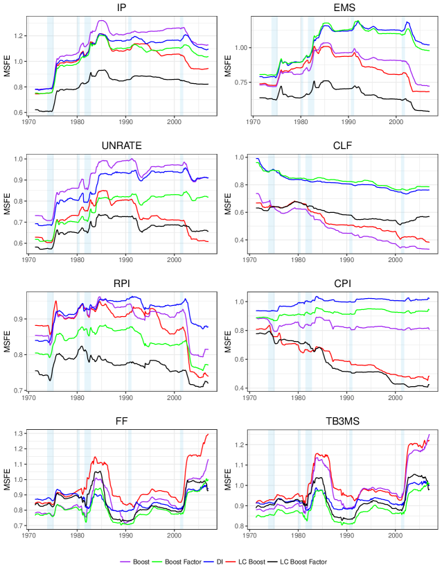
Figure 1: MSFE by start date of out of sample period. Horizon $h=12$. More specifically we plot: $MSFE^{12}_{(i)}(T_{1},T_{2})=\sum_{t=T_{1}}^{T_{2}}\hat{\epsilon}^{2}_{t,(i)}/\sum_{t=T_{1}}^{T_{2}}\hat{\epsilon}^{2}_{t,(AR)}$, where we $T_{1}$ vary from 1971:9 until 2006:12, with $T_{2}$=2018:8. Shaded regions represent NBER recession dates.

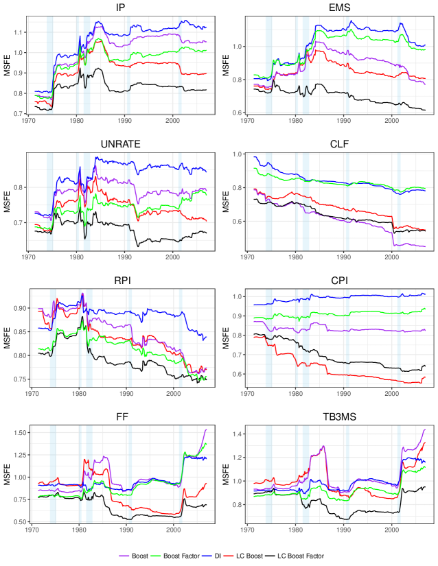
Figure 2: MSFE by start date of Out of sample period. Horizon $h=6$. See notes to figure 1.

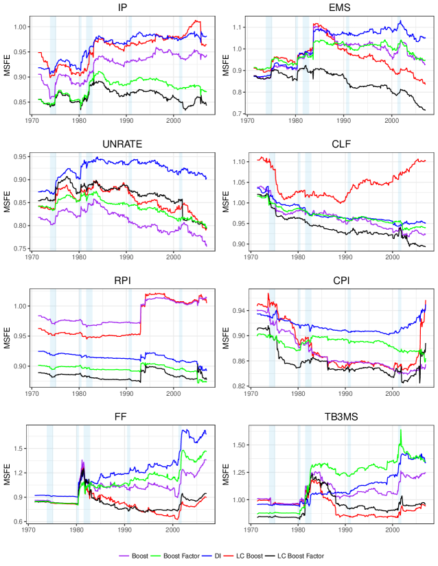
Figure 3: MSFE by start date of out of sample period. Horizon $h=1$. See notes to figure 1.

For the first method, we let $T_{1}$ vary from 1971:9 until 2006:12. We plot the MSFE by $T_{1}$ for the top 5 performing methods: LC-Boost Factor, LC-Boost, Boost, Boost Factor, and DI. The figures 1-3; contain the results for horizons $h=12,6,1$ respectively. Looking at figures 1-3, we see that LC-Boost Factor is easily the best performing method for horizon $h=12,6$, and to a lesser extent $h=1$. Comparing across all horizons, we notice:

• The performance improvements for LC-Boost factor, relative to its time invariant counterparts, are more apparent as we increase the forecast horizon.

• As we increase $T_{1}$, the gap between LC-Boost Factor and the time invariant methods widens. In particular we notice a large separation in performance starting during great moderation period.

Additionally, we also observe that the commonly used DI model loses much of its predictive ability during the Great moderation and performs worse than the benchmark for about half of the series. This result suggests that DI gained most of its predictability vs the benchmark during the “Pre-Great Moderation” period.

Table 2 contain the results for each of the subperiods for horizon $h=12$; the corresponding results for $h=6,3,1$ are found in the appendix. For each subperiod we report the MSFE, relative to the MSFE of the benchmark AR(4) model. We start with the “Pre-Great Moderation” period, and note that with the exception of TV-AR models, all other models strongly outperform the benchmark model the majority of the time during this period. Time invariant methods such as Boost Factor and DI models perform best, and their performance is strongest when forecasting at longer horizons. LC-Boost factor appears to be slightly lag behind these two methods during this time period. As we enter the “Great Moderation” period, the performance of all models generally declines relative to the AR benchmark. In particular, time invariant methods such as DI and Boost take a large hit and underperform the benchmark in many cases, especially for $h=12$. LC-Boost Factor undergoes a much smaller decline compared to the rest of the models, and emerges as the best performing model during this time period. Importantly, we also observe that LC-Boost performs at the same level or worse than its time invariant counterpart Boost in the majority of cases. This suggests that although there seems to be a large amount of time variation in this period, the bias variance tradeoff in modeling it is not favorable to a model with a large amount of potential predictors ($\sim 500$ predictors). During the “Post Great Moderation” period the performance of LC-Boost methods show large improvements relative to the benchmark AR model, and relative to their time invariant counterparts, for all forecast horizons, with the improvement being greatest for longer horizons.

8.2 Assessing Benefits of Modeling Time Varying Parameters

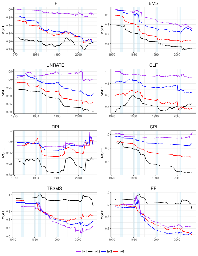
Figure 4: MSFE of LC-Boost Factor (LC-BF) relative to MSFE of Boost Factor (BF) by start date of out of sample period: Figure plots $MSFE_{(LC-BF)}(T_{0},T_{2})/MSFE_{(BF)}(T_{0},T_{2})$ for $T_{0}=\text{1971:9},\ldots,\text{2006:12}$ and $T_{2}=\text{2018:8}$. See notes to figure 1 or equation (10) for details. Colored lines represent the different horizons. Shaded regions represent NBER recession dates.

In order to assess the benefits of directly modeling parameter instability, we compare the performance of LC-Boost Factor vs Boost-Factor. These also happen to be the best time varying and time invariant methods respectively. We start our analysis by first plotting the MSFE of LC-Boost Factor, relative to the MSFE of Boost Factor, as a function of the start date for the out of sample forecast period, i.e. $MSFE_{(LCBoostFactor)}(T_{1},T_{2})/MSFE_{(BoostFactor)}(T_{1},T_{2})$. The results are in figure 4. We observe that for all series and forecast horizons LC-Boost Factor almost never performs worse than Boost Factor, and outperforms it the vast majority of the time. Furthermore, the gap between the two methods widens as we increase $T_{1}$, the start date of the out of sample period, and as we increase $h$, the forecast horizon. For example, if we consider horizon $h=12$, and we start the out of sample period in the early 1990’s, LC Boost offers, on average, over a 20 percent improvement over Boost-Factor. We observe similar patterns, although the improvements are not as large ($\sim$ 10-15 percent on average), for horizons $h=3,6$. An exception seems to be for $h=1$, which shows little improvements for the majority of series, with the exceptions coming from the two interest rate series and EMS.

Next, we attempt to get a finer look at how the benefits of modeling parameter instability vary over time. We first define the local MSFE (L-MSFE), of method $i$ at time $t_{0}$ as :

$$\text{L-MSFE}_{i}(t_{0})=\frac{\sum_{t=t_{0}-\Delta}^{t_{0}+\Delta}\hat{\epsilon}_{t,(i)}^{2}}{\sum_{t=t_{0}-70}^{t_{0}+\Delta}\hat{\epsilon}_{t,(AR)}^{2}},\quad\quad\text{RL-MSFE}_{i}(t_{0})=\frac{\text{L-MSFE}_{i}(t_{0})}{\text{L-MSFE}_{\text{BoostFactor}}(t_{0})}$$

with the convention that $\hat{\epsilon}_{t,(i)}=0$ for $t\leq 0,t\geq T$. This amounts to using a uniform kernel to weight the forecast errors with a bandwidth chosen such that the window size has $\Delta=70$ observations. We then plot $\text{RL-MSFE}_{i}(t_{0})$ for $i=$LCBoostFactor, for $t_{0}=\text{1977:3},\ldots,\text{2012:10}$ for all series and forecast horizons. The endpoints are chosen so that the first and last values in the plot correspond to the RL-MSFE during the “Pre-Great Moderation” and “Post-Great Moderation” periods respectively.

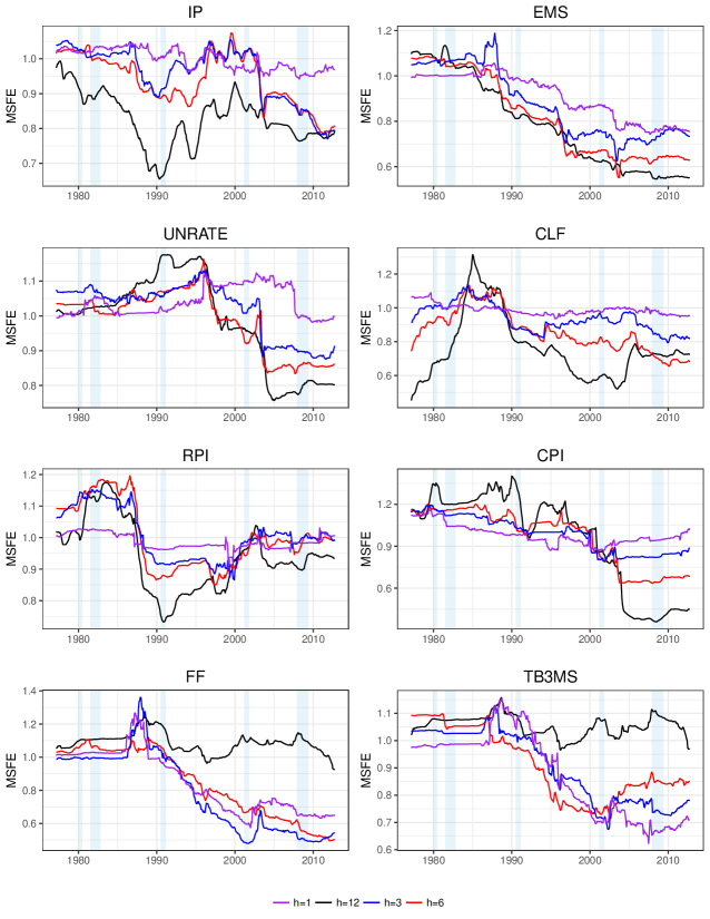
Figure 5: Local MSFE of LC-Boost Factor relative to Local MSFE of Boost Factor: To obtain the local MSFE of a model we use a rolling mean with a window size of 70 observations, which gives us: $\text{L-MSFE}_{i}(t_{0})=\sum_{t=t_{0}-70}^{t_{0}+70}\hat{\epsilon}_{t,(i)}^{2}/\sum_{t=t_{0}-70}^{t_{0}+70}\hat{\epsilon}_{t,(AR)}^{2}$ with the convention that $\hat{\epsilon}_{t,(i)}=0$ for $t\leq 0,t\geq T$. We then plot $\text{L-MSFE}_{LCBoostFactor}(t)/\text{L-MSFE}_{BoostFactor}(t)$, for $t=\text{1977:3},\ldots,\text{2012:10}$

The results are in figure 5, and we observe that the first value is usually near or above one for all variables except for CLF (Civilian Labor Force). This suggests that during the “Pre-Great Moderation” there seems to be little or no benefit to modeling time variation. This can reflect either a lack of underlying parameter instability during this time period, or the relatively low sample size available combined with high volatility made it difficult to exploit the time variation present. During the Great Moderation period, almost all series experience large declines in RL-MSFE, with the exact timing of the decline differing by series. For IP and RPI the benefits to modeling parameter instability appear to decrease from their mid 1990’s levels, while for the rest of the series we see further improvements until the end of the sample. These results suggest that there is a large amount of parameter instability which started during the Great moderation period and continued though the sample.

Lastly, we attempt to examine the degree and timing of time variation by examining the bandwidth values selected. We define the local bandwidth of LC-Boost Factor as: $\text{L-BW}(t_{0})=\sum_{t=t_{0}-\Delta}^{t_{0}+\Delta}\hat{b}_{t_{0}}/(2\Delta)$, with the convention that $\hat{b}_{t_{0}}=0$ for $t\leq 0,t\geq T$. Recall that $\hat{b}_{t_{0}}$ is the bandwidth chosen at time $t_{0}$. Since we are using the uniform kernel, $\hat{b}_{t_{0}}$ represents the fraction of the sample available at time $t_{0}$ that we are using for estimation. As as example, at time $t_{0}$=1977:3 we have a total of 196 observations available for estimation, therefore a value of $\hat{b}_{t_{0}}=.61$ for $t_{0}$=1977:3 implies we are using $\approx$ 120 observations. We set $\Delta=70$ observations, and then plot $\text{L-BW}(t_{0})$ for $t_{0}=\text{1977:3},\ldots,\text{2012:10}$ for all series and forecast horizons. As an additional comparison we also plot the local bandwidth implied by a rolling window estimator which uses a fixed window length of 120 observations. We also note that $b_{t_{0}}=1$ for Boost Factor at all time points, since it uses the entire sample available at time $t_{0}$.

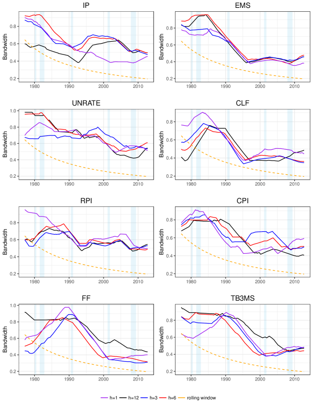
Figure 6: Local Bandwidth of LC-Boost Factor: To obtain the local bandwidth of LC-Boost Factor we use a rolling mean with a window size of 70 observations, which gives us: $\text{L-BW}_{i}(t_{0})=\sum_{t=t_{0}-70}^{t_{0}+70}\hat{b}_{t,(i)}/140$ for $i=$LC-Boost Factor. We also include the local bandwidth implied by a rolling window estimator which uses the last 120 observations

The results are seen in figure 6, and we notice that for the pre Great Moderation period the local bandwidths are usually between .7-.8 for most series. As we enter the Great Moderation we notice that the local Bandwidths generally tend to increase initially before declining. However, we notice the timing and degree of declines differs by series. For some series such as IP and RPI, the local BW tends to increase after reaching their lows in the mid 1990s, whereas for other series such as UNRATE, FEDFUNDS, and TB3MS the local BW start their decline in the 1990s. In contrast, we see that using a fixed rolling window of 120 observations implies a monotonically decreasing bandwidth and assumes the same bandwidth regardless of series or horizon. To determine the importance of estimating the optimal bandwidth via cross valiation, we compare the local MSFE of LC-Boost Factor to Boost Factor estimated using a 120 observation rolling window in the appendix. The results show that for the vast majority of series and horizons the rolling window estimator is strongly outperformed by LC-Boost Factor with the largest gains occurring during the Great Moderation period.

Overall our results suggest the following conclusions:

1. Parameter instability starts to appear around the beginning of the Great Moderation period. This instability seriously deteriorates the relative forecasting performance of time invariant methods; with the effect being more severe for longer horizon forecasts.

2. Due to the large improvements in point forecasts from our methods, it is likely that this instability has a substantial impact on the conditional mean as well as the conditional variance of various economic series.

3. The commonly used rolling window estimation method can understate the benefits of modeling parameter instability by failing to account for differences in the degree of parameter instability by series, forecast horizon, and time period.

4. Lastly, there are large benefits to modeling parameter instability if done properly. Given the high bias variance tradeoff encountered in using a reduced sample size, these benefits can easily be missed. For example, models such as LC-Boost have more difficulty in learning the time variation in the data due to the large amount of potential predictors.

To elaborate more on point 4) above, we also compare the L-MSFE of the following models in the appendix: LL-Boost Factor vs LC-Boost Factor, LC-Boost vs LC-Boost Factor, and LC-Boost vs Boost. We see from the results that LL-Boost Factor was strongly outperformed by LC-Boost Factor in the earlier parts of the sample, suggesting that there was little time variation during the pre-great Moderation period. As our sample size available for estimation increases and as the time variation starts to become more apparent, we see the performance of LL-Boost factor improve to the point where it does as well as or outperforms LC-Boost factor in about half of the series, especially for longer horizons. Compared to LC-Boost Factor, we observe that the benefits of modeling time variation via LC-Boost are smaller and are realized far later in the sample. As an example, for $h=12$ we notice that LC-Boost performs worse than Boost during most of the Great moderation period. Additionally, for many of the series, the improvements of LC-Boost over Boost start to occur near the end of the great moderation period. In contrast, LC-Boost Factor is able to adapt to the time variation far earlier as a result of having a more favorable bias variance tradeoff.

9 Conclusion

In this work, we have presented two $L_{2}$ Boosting algorithms for estimating high dimensional predictive regressions with time varying coefficient. We proved the consistency of both of these methods, and showed their effectiveness in modeling the parameter instability present in macroeconomic series. Compared to other TVP methods, our methods are very efficient computationally even for high dimensional data; a single LC-Boost forecast, including implementing the cross validation procedure, can be estimated within a matter of seconds. Additionally, they can be implemented by researchers and practitioners using the easy to use R package mboost. Furthermore, the boosting framework can be easily adapted to fitting more complex non-linear models.

There are many topics available for further study, one such topic is in selecting the important bandwidth parameter for our models. Although our cross validation procedure seems to perform adequately, we welcome further improvements to this methodology. Lastly, although our empirical example focused on forecasting, our models are applicable in a far broader range of settings.

Table 2: Relative MSFE $h=12$

Full Out of Sample Period 1971:9-2018:8
	IP	PAYEMS	UNRATE	CLF	RPI	CPI	FF	TB3MS
TV-AR	1.04	.99	1.1	.64	.99	.86	1	1.07
DI	.79	.79	.69	.99	.84	.94	.87	.91
Lasso	.77	.81	.75	.77	.93	.96	.76	.89
Boost	.78	.73	.73	.74	.85	.88	.79	.88
Boost Factor	.75	.81	.62	.96	.80	.89	.78	.85
LC-Boost	.74	.73	.62	.66	.88	.80	.85	.92
LC-Boost Factor	.62	.64	.58	.63	.75	.77	.84	.90
LL-Boost Factor	.74	.85	.70	.76	.76	.82	1.20	1.37

“Pre-Great Moderation” 1971:9-1982:12
	IP	PAYEMS	UNRATE	CLF	RPI	CPI	FF	TB3MS
TV-AR	1.07	1	1.15	.71	.96	1.11	1.01	1.14
DI	.38	.49	.48	1.51	.61	82	.88	.89
Lasso	.30	.51	.41	1.27	.71	1.13	.76	.77
Boost	.27	.44	.43	1.24	.67	.92	.72	.75
Boost Factor	.32	.50	.43	1.34	.65	.84	.74	.80
LC-Boost	.29	.44	.38	.86	.77	1.03	.70	.79
LC-Boost Factor	.31	.54	.43	.60	.66	.94	.77	.81
LL-Boost Factor	.41	.83	.66	.86	.80	1.04	1.28	1.57

“Great Moderation” 1983:1-2006:12
	IP	PAYEMS	UNRATE	CLF	RPI	CPI	FF	TB3MS
TV-AR	1.12	1	1.11	.65	1.06	1.07	1.04	1.03
DI	1.18	1.08	.75	.88	1	1	.85	.92
Lasso	1.23	1.32	.97	.85	1.10	.90	.80	1.03
Boost	1.36	1.20	.95	.81	1.08	.91	.85	1
Boost Factor	1.25	1.16	.67	.89	1	.90	.80	.90
LC-Boost	1.43	1.26	.97	.82	1.16	.90	1.07	1.05
LC-Boost Factor	.99	.89	.71	.71	.89	1	.97	1.01
LL-Boost Factor	1.03	1	.79	.90	.86	1.14	1.16	1.22

“Post Great Moderation” 2007:1-2018:8
	IP	PAYEMS	UNRATE	CLF	RPI	CPI	FF	TB3MS
TV-AR	.96	.98	1	.58	.96	.41	.79	.83
DI	1.10	1.02	.91	.76	.88	1.02	.94	1
Lasso	1.15	.76	.99	.36	.95	.79	.89	1.07
Boost	1.13	.72	.91	.33	.81	.81	1.13	1.25
Boost Factor	1.04	.98	.82	.79	.77	.94	1	1.01
LC-Boost	.94	68	.60	.38	.73	.48	1.29	1.21
LC-Boost Factor	.82	.54	.66	.57	.72	.42	.92	.98
LL-Boost Factor	1.01	.69	.66	.55	.66	.33	.56	.67

Appendix: Proofs

Proof of Theorem 1(a).

The proof follows the framework of Buhlmann (2006), which handled the case of boosting for iid data using linear least squares base learners. The proof depends on an application of Temlyakov’s result (Temlyakov, 2000) for the population version of $L_{2}$ boosting known as “weak greedy algorithm”. We start by considering a step size of $\nu=1$, and smaller step sizes can be handled as in section 6.3 of Buhlmann (2006).

Throughout this section let $C,c$ refer to generic constants which can change from line to line. We introduce the following notation: Let $\bm{\tilde{x}}_{t-h}(u)$ and $\tilde{Y}_{t}(u)$ be the stationary approximation to $\bm{x}_{t-h,T}$ and $Y_{t,T}$ respectively with approximation error $O_{p}(T^{-1})\rightarrow 0$. Let the inner product $\big{\langle}\tilde{X}_{j,t}(u),\tilde{X}_{k,t}(u)\big{\rangle}=E(\tilde{X}_{j}(u)\tilde{X}_{k}(u))$ with $||\tilde{X}_{j}(u)||^{2}=E(\tilde{X}^{2}_{j}(u))$. For ease of presentation let $||\tilde{X}_{j}(u)||^{2}=1$, $\forall j\leq p_{T}$, we will expand on this in more detail later, but we note that we are not using loss of generality by this assumption. We can define a new scaled process for each $u\in[0,1]$ as $\tilde{X}^{*}_{j,t}(u)=\tilde{X}_{j,t}(u)/||\tilde{X}_{j}(u)||$. However, we note that we are still placing all our assumptions on the unscaled process i.e weak dependence, smoothness, locally stationary approximation to $X_{j,uT,T}$ etc.

Let $f(u,\bm{\tilde{x}}_{t-h}(u))=\tilde{\bm{x}}_{t-h}(u)\bm{\beta}(u)$ be the stationary approximation to $f(u,\bm{x}_{t-h,T})$ with approximation error $O_{p}(T^{-1})$. For readability, we define, for any rescaled time point $u\in[0,1]$:

$$f(\tilde{\bm{x}}_{uT-h}(u))\equiv f(u,\tilde{\bm{x}}_{uT-h}(u)),\text{and }f(\bm{x}_{uT-h,T})\equiv f(u,\bm{x}_{uT-h,T}).$$

We now define a sequence of remainder functions for the population version of $L_{2}$ Boosting:

$$R^{0}f(\tilde{\bm{x}}_{uT-h}(u))=f(\tilde{\bm{x}}_{uT-h}(u)),$$

$$R^{m}f(\tilde{\bm{x}}_{uT-h}(u))=R^{m-1}f(\tilde{\bm{x}}_{uT-h}(u))-\big{\langle}R^{m-1}f(\tilde{\bm{x}}_{uT-h}(u)),\tilde{X}_{\mathcal{S}_{m},uT-h}(u)\big{\rangle}\tilde{X}_{\mathcal{S}_{m},uT-h}(u),m=1,2,\ldots$$

Where $\mathcal{S}_{m}=\mbox{argmax}_{j}|\big{\langle}R^{m-1}f(\tilde{\bm{x}}_{uT-h}(u)),\tilde{X}_{j,uT-h}(u)\big{\rangle}|$. Given that this criterion is sometimes infeasible to realize in practice, a weaker criterion is: Choose any $\mathcal{S}_{m}$ which satisfies:

$$|\big{\langle}R^{m-1}f(\tilde{\bm{x}}_{uT-h}(u)),\tilde{X}_{\mathcal{S}_{m}}(u)\big{\rangle}|\geq b*\sup_{j}|\big{\langle}R^{m-1}f(\tilde{\bm{x}}_{uT-h}(u)),\tilde{X}_{j}(u)\big{\rangle}|,\text{ for some }b\in(0,1]$$ (11)

We then obtain:

$$f(\tilde{\bm{x}}_{uT-h}(u))=\sum_{j=0}^{m-1}\big{\langle}R^{j}f(\tilde{\bm{x}}_{uT-h}(u)),\tilde{X}_{\mathcal{S}_{j+1}}(u)\big{\rangle}+R^{m}f(\tilde{\bm{x}}_{uT-h}(u)),$$

$$||R^{m}f(\tilde{\bm{x}}_{uT-h}(u))||^{2}=||R^{m-1}f(\tilde{\bm{x}}_{uT-h}(u))||^{2}-|\big{\langle}R^{m-1}f(\tilde{\bm{x}}_{uT-h}(u)),\tilde{X}_{\mathcal{S}_{m}}(u)\big{\rangle}|^{2}$$

If (11) is met, then we have the following bound, for the population version of $L_{2}$ Boosting, provided by Temlyakov (2000):

$$||R^{m}f(\tilde{\bm{x}}_{uT-h}(u))||^{2}\leq B(1+mb^{2})^{\frac{-b}{4+2b}}$$ (12)

with as defined in (11), and $\sup_{u\in[0,1]}|\bm{\beta}(u)|\leq B<\infty$.

To analyze the sample version of our LC-Boost algorithm, we introduce the following notation:

$$\big{\langle}X_{j,\cdot,T},X_{k,\cdot,T}\big{\rangle}_{(T)}=\sum_{t=1}^{T}K_{b}(t/T-u)X_{j,t-h,T}X_{k,t-h,T}$$

$$\big{\langle}f,X_{k,\cdot,T}\big{\rangle}_{(T)}=\sum_{t=1}^{T}K_{b}(t/T-u)f(\bm{x}_{t-h})X_{k,t-h,T}$$

$$||X_{j,\cdot,T}||^{2}_{(T)}=\sum_{t=1}^{T}K_{b}(t/T-u)X_{j,t-h,T}^{2}$$

We suppress the dependence on $u$ in the notation above. We assume that $||X_{j,\cdot,T}||_{(T)}=1$, and once again we do not lose any generality from this. We can define a new scaled process for each $u\in[0,1]$ as ${X^{*}_{j,t,T}(u)}_{t=1,\ldots,T}={X_{j,t,T}/||X_{j,\cdot,T}||_{(T)}}_{t=1,\ldots,T}$. As before we are not placing any assumptions such as local stationarity or weak dependence on this scaled process, and we show that our results hold only from the assumptions placed on the unscaled process $X_{j,t,T}$. The key will be the uniform concentration bounds derived in lemma 1. As previously, we can define the sequence of sample remainder functions as:

$$\hat{R}_{T}^{0}f(\bm{x}_{uT-h,T})=f(\bm{x}_{uT-h,T}),$$

$$\hat{R}_{T}^{m}f(\bm{x}_{uT-h,T})=\hat{R}_{T}^{m-1}f(\bm{x}_{uT-h,T})-\big{\langle}\hat{R}_{T}^{m-1}f,X_{\widehat{\mathcal{S}}_{m},\cdot,T}\big{\rangle}_{(T)}X_{\widehat{\mathcal{S}}_{m},uT-h,T},m=1,2,\ldots$$

where: $\hat{\mathcal{S}}_{1}=\mbox{argmax}_{j}|\langle Y_{\cdot,T},X_{j,\cdot,T}\rangle_{(T)}|$ and $\hat{\mathcal{S}}_{m}=\mbox{argmax}_{j}|\langle\hat{R}_{T}^{m}f,X_{j,\cdot,T}\rangle_{(T)}|$. Therefore, $\hat{R}_{T}^{m}f(\bm{x}_{uT-h,T})=f(\bm{x}_{uT-h,T})-\hat{F}_{lc}^{(M_{T})}(u,\bm{x}_{uT-h,T})$, is the difference between $f(\bm{x}_{uT-h,T})$ and its LC-Boost estimate.

Lastly, to proceed with the proof, we define a sequence of semi-population version remainder functions as:

$$\tilde{R}_{T}^{0}f(\tilde{\bm{x}}_{uT-h}(u))=f(\tilde{\bm{x}}_{uT-h}(u)),$$

$$\tilde{R}_{T}^{m}f(\tilde{\bm{x}}_{uT-h}(u))=\tilde{R}_{T}^{m-1}f(\tilde{\bm{x}}_{uT-h}(u))-\big{\langle}\tilde{R}_{T}^{m-1}f(\tilde{\bm{x}}_{uT-h}(u)),\tilde{X}_{\widehat{\mathcal{S}}_{m},uT-h}(u)\big{\rangle}\tilde{X}_{\widehat{\mathcal{S}}_{m},uT-h}(u),m=1,2,\ldots$$

The difference between the population and the semi-population remainder functions, is that the semi-population version uses selectors $\hat{\mathcal{S}}_{m}$ estimated from the sample. The strategy of the proof is: first we establish that the selectors $\hat{\mathcal{S}}_{m}$ satisfy a finite sample analogue of (11), which allows us to apply Temlyakov’s result (12) to the semipopulation version. Lastly, we analyze the difference between the sample and the semipopulation versions: $\hat{R}_{T}^{m}f(\bm{x}_{uT-h,T})-\tilde{R}_{T}^{m}f(\tilde{\bm{x}}_{uT-h}(u))$.

We need the following lemma:

Lemma 1.

Under conditions 5.1, 5.2, 5.3, 5.4, and for $\kappa$ as defined in Theorem 1, the following hold:

1. $\sup_{j,k\leq p_{T}}\sup_{u\in[0,1]}|\sum_{t=1}^{T}K_{b}(t/T-u)X_{j,t,T}X_{k,t,T}-E(\tilde{X}_{j,T}(u)\tilde{X}_{k,T}(u))|=\zeta_{T,1}=O_{p}(S_{T}^{-\kappa})$
   

2. $\sup_{j\leq p_{T}}\sup_{u\in[0,1]}|\sum_{t=1}^{T}K_{b}(t/T-u)X_{j,t-h,T}\epsilon_{t,T}|=\zeta_{T,2}=O_{p}(S_{T}^{-\kappa})$
   

3. $\sup_{j\leq p_{T}}\sup_{u\in[0,1]}|\sum_{t=1}^{T}K_{b}(t/T-u)X_{j,t,T}f(\bm{x}_{t,T})-E(\tilde{X}_{j,T}(u)f(\tilde{\bm{x}}_{T}(u)))|=\zeta_{T,3}=O_{p}(S_{T}^{-\kappa})$
   

4. $\sup_{j\leq p_{T}}\sup_{u\in[0,1]}|\sum_{t=1}^{T}K_{b}(t/T-u)X_{j,t-h,T}Y_{t,T})-E(\tilde{X}_{j,t-h}(u)\tilde{Y}_{T}(u)))|=\zeta_{T,4}=O_{p}(S_{T}^{-\kappa})$

Now we note that using the above lemma we can bound sums of the form:

$$\sup_{u\in[0,1]}\sup_{j}|\sum_{t=1}^{T}K_{b}(t/T-u)X_{j,t-h,T}Y_{t,T}/||X_{j,\cdot,T}||_{(T)}-E(\tilde{X}_{j,t-h}(u)\tilde{Y}_{T}(u)))/||\tilde{X}_{j,t-h}(u)|||$$

if we assumed that $||\tilde{X}_{j,t}(u)||,||X_{j,t-h,T}||_{(T)}\neq 1$.

Let $\zeta_{T}=\max(\zeta_{T,1},\zeta_{T,2},\zeta_{T,3},\zeta_{T,4})=O_{p}(S_{T}^{-\kappa})$ and denote by $\omega$ a realization of all $T$ sample points involved in estimation. The next lemma bounds the difference between the sample and population learners at step $m$.

Lemma 2.

Suppose conditions 5.1, 5.2, 5.3, and 5.4 hold. Then for $\kappa$ as defined in Theorem 1 and on the set $\mathcal{A}_{T}=\{\omega:\zeta_{T}(w)<1/2\}$, we have:

$$\sup_{u\in[0,1]}\sup_{j\leq p_{T}}|\big{\langle}\hat{R}^{m-1}f,X_{j,\cdot,T}\big{\rangle}_{(T)}-\big{\langle}\tilde{R}^{m-1}f(\tilde{\bm{x}}_{uT-h}(u)),\tilde{X}_{j,uT-h}(u)\big{\rangle}|\leq C(5/2)^{m}\zeta_{T},$$

where $C$ does not depend on $m,T$.

It’s clear from lemma 1, that $P(\mathcal{A}_{T})\rightarrow 1$. Which gives us the following lemma:

Lemma 3.

Suppose the conditions needed for lemma 1 hold, then for $m=m_{T}\rightarrow\infty$ slow enough we have:

$$\sup_{u\in[0,1]}||\tilde{R}_{T}^{m}f(\tilde{\bm{x}}_{uT-h}(u))||=o_{p}(1)$$

We now analyze the term: $\hat{R}_{T}^{m}f(\bm{x}_{uT-h,T})=f(\bm{x}_{uT-h,T})-\hat{F}_{lc}^{(M_{T})}(u,\bm{x}_{uT-h,T})$. By the triangle inequality we obtain:

$$||\hat{R}_{T}^{m}f(\bm{x}_{uT-h,T})||\leq||\tilde{R}_{T}^{m}f(\tilde{\bm{x}}_{uT-h}(u))||+||\hat{R}_{T}^{m}f(\bm{x}_{uT-h,T})-\tilde{R}_{T}^{m}f(\tilde{\bm{x}}_{uT-h}(u))||$$ (13)

the first term can be handled with lemma 3. For the second term, let $A_{T}(m)=||\hat{R}_{T}^{m}f(\bm{x}_{uT-h,T})-\tilde{R}_{T}^{m}f(\tilde{\bm{x}}_{uT-h}(u))||$. Using the definitions of the remainder functions, we then have a recursive relation:

$$A_{T}(m) \leq A_{T}(m-1)+|\big{\langle}\hat{R}^{m-1}f,X_{\widehat{\mathcal{S}}_{m},\cdot,T}\big{\rangle}_{(T)}-\big{\langle}\tilde{R}^{m-1}f,\tilde{X}_{\widehat{\mathcal{S}}_{m},uT-h}\big{\rangle}|||X_{\widehat{\mathcal{S}}_{m},uT-h,T}||$$

$$+||\big{\langle}\tilde{R}^{m-1}f,\tilde{X}_{\widehat{\mathcal{S}}_{m},uT-h}\big{\rangle}||||X_{\widehat{\mathcal{S}}_{m},uT-h,T}-\tilde{X}_{\widehat{\mathcal{S}}_{m},uT-h}(u)||$$

$$\leq A_{T}(m-1)+C(5/2)^{m}\zeta_{T}+C/T\text{ on the set }\mathcal{A}_{T}$$

where the above inequality holds uniformly over all $u\in[0,1]$. The last inequality follows from local stationarity and lemma 2. By the above recursive equation we obtain: $\sup_{u\in[0,1]}||\hat{R}_{T}^{m}f(\bm{x}_{uT-h,T})-\tilde{R}_{T}^{m}f(\tilde{\bm{x}}_{uT-h}(u))||\leq 3^{m}\zeta_{T}C\text{ on the set }\mathcal{A}_{T}$. If we choose $m=m_{T}\rightarrow\infty$ slow enough (e.g $m_{T}=o(log(T))$), then along with lemma 3 and (13) we obtain:

$$\sup_{u\in[0,1]}||\hat{R}_{T}^{m}f(\bm{x}_{uT-h,T})||=\sup_{u\in[0,1]}||f(\bm{x}_{uT-h,T})-\hat{F}_{lc}^{(M_{T})}(u,\bm{x}_{uT-h,T})||=o_{p}(1)$$

∎

Online Appendix to Boosting High Dimensional Predictive Regressions with Time Varying Parameters

1 Online Appendix A: Additional Proofs

Proof of Lemma 1.

We start with (i), and we bound:

$$P(\sup_{u\in[0,1]}|\sum_{t=1}^{T}K_{b}(t/T-u)X_{j,t,T}X_{k,t,T}-E(\tilde{X}_{j,T}(u)\tilde{X}_{k,T}(u))|>S_{T}^{-\kappa})$$ (A.1)

$$\leq P\bigg{(}\sup_{u\in[0,1]}|\sum_{t=1}^{T}K_{b}(t/T-u)[X_{j,t,T}X_{k,t,T}-E(X_{j,t,T}X_{k,t,T})]|$$ (A.2)

$$+|\sup_{u\in[0,1]}|\sum_{t=1}^{T}K_{b}(t/T-u)E(X_{j,t,T}X_{k,t,T})-E(\tilde{X}_{j,T}(u)\tilde{X}_{k,T}(u))|>S_{T}^{-\kappa}\bigg{)}$$ (A.3)

We deal with the second term, which can be thought of as the bias. The product process $X_{j,t,T}X_{k,t,T}$ is locally stationary with the stationary approximation at rescaled time $t/T$ being $\tilde{X}_{j,t}(t/T)\tilde{X}_{k,t}(t/T)$. One can see this by noting:

$$||\tilde{X}_{j,T}(u)\tilde{X}_{k,T}(u))-\tilde{X}_{j,T}(v)\tilde{X}_{k,T}(v))||_{r/2} \leq(||\tilde{X}_{j,T}(u)||_{r}||\tilde{X}_{k,T}(u)-\tilde{X}_{k,T}(v)||_{r}$$

$$+||\tilde{X}_{k,T}(u)||_{r}||\tilde{X}_{j,T}(u)-\tilde{X}_{j,T}(v)||_{r})$$

$$\leq C(|u-v|)$$

which holds uniformly in $u,v\in[0,1]$. We can employ the same techniques to that $||X_{j,t,T}X_{k,t,T}-\tilde{X}_{j,t}(t/T)\tilde{X}_{k,t}(t/T)||\leq C(T^{-1})$.

Therefore by local stationarity we obtain:

$$|\sup_{u\in[1-b_{T},1]}\sum_{t=1}^{T}K_{b}(t/T-u)E(X_{j,t,T}X_{k,t,T})-E(\tilde{X}_{j,T}(u)\tilde{X}_{k,T}(u))|\leq O(S_{T}/T)$$ (A.4)

Note that if $u$ is an interior point (i.e $u\in(b_{T},1-b_{T})$ where $b_{T}$ is the bandwidth), the bound improves to $O((S_{T}/T)^{2})$. Let $\tilde{\sigma}_{jk}(u)=E(\tilde{X}_{j,t}(u)\tilde{X}_{k,t}(u))$, then by condition 5.3, we obtain:

$$\tilde{\sigma}_{jk}(t/T)=\tilde{\sigma}_{jk}(u)+\tilde{\dot{\sigma}}_{jk}(u)(t/T-u)+O(b_{T}^{2})$$

where $\tilde{\dot{\sigma}}_{jk}(u)$ refers to the derivative of the covariance matrix w.r.t the rescaled time index. This gives us:

$$|\sup_{u\in(b_{T},1-b_{T})}|\sum_{t=1}^{T}K_{b}(t/T-u)E(X_{j,t,T}X_{k,t,T})-E(\tilde{X}_{j,T}(u)\tilde{X}_{k,T}(u))|\leq O((S_{T}/T)^{2})$$ (A.5)

Now we deal with the term (A.2), note that the functional dependence measure of the stationary approximation Using this we compute the functional dependence measure of $\tilde{X}_{j,T}(u)\tilde{X}_{k,T}(u))$ as:

$$\sup_{u\in[0,1]}||\tilde{X}_{j,T}(u)\tilde{X}_{k,T}(u))-\tilde{X}_{j,T}^{*}(u)\tilde{X}_{k,T}^{*}(u))||_{r/2} \leq\sup_{u\in[0,1]}(||\tilde{X}_{j,T}(u)||_{r}||\tilde{X}_{k,T}(u)-\tilde{X}_{k,T}(u)^{*}||_{r}$$ (A.6)

$$+\sup_{u\in[0,1]}||\tilde{X}_{k,T}(u)||_{r}||\tilde{X}_{j,T}(u)-\tilde{X}_{j,T}(u)^{*}||_{r})$$

Therefore, $\tilde{X}_{j,T}(u)\tilde{X}_{k,T}(u)$ has a finite cumulative dependence measure by the weak dependence condition imposed on $\bm{\tilde{x}}_{t}(u)$. Taking into account (A.4), and the above we can then apply theorem 2.7 (iii) in Dahlhaus et al. (2018) to obtain:

$$P(\sup_{u\in[0,1]}|\sum_{t=1}^{T}K_{b}(t/T-u)X_{j,t,T}X_{k,t,T}- E(\tilde{X}_{j,T}(u)\tilde{X}_{k,T}(u))|>S_{T}^{-\kappa})$$

$$\leq O(TS_{T}^{-r/2+r\kappa/2})+O(\exp(-S_{T}^{1-2\kappa}))$$

Applying the union bound then completes the proof.

For (ii), we proceed similarly. Given that $E(X_{j,t-h,T}\epsilon_{t,T})=0,\text{ }\forall j$. We have that $E(\tilde{X}_{j,t-h}(u)\tilde{\epsilon}_{T}(u))=O(T^{-1})$. We bound:

$$P\bigg{(}\sup_{u\in[0,1]}|\sum_{t=1}^{T}K_{b}(t/T-u)X_{j,t-h,T}\epsilon_{t,T}-E(\tilde{X}_{j,t-h}(u)\tilde{\epsilon}_{T}(u))|>S_{T}^{-\kappa}\bigg{)}$$ (A.7)

$$\leq P\bigg{(}\sup_{u\in[0,1]}|\sum_{t=1}^{T}K_{b}(t/T-u)X_{j,t-h,T}\epsilon_{t,T}|>O(S_{T}^{-\kappa})\bigg{)}$$ (A.8)

Now we apply the same procedure as previously. We have that:

$$\sup_{u\in[0,1]}||\tilde{X}_{j,t}(u)\tilde{\epsilon}_{t}(u))-\tilde{X}_{j,t}^{*}(u)\tilde{\epsilon}_{t}^{*}(u))||_{\tau} \leq\sup_{u\in[0,1]}(||\tilde{X}_{j,t}(u)||_{r}||\tilde{\epsilon}_{t}(u)-\tilde{\epsilon}_{t}(u)^{*}||_{q}$$ (A.9)

$$+\sup_{u\in[0,1]}||\tilde{\epsilon}_{t}(u)||_{q}||\tilde{X}_{j,t}(u)-\tilde{X}_{j,t}(u)^{*}||_{r})$$

This has a finite cumulative functional dependence measure by the weak dependence conditions imposed. Once again, by applying theorem 2.7 (iii) in Dahlhaus et al. (2018) we obtain:

$$P(\sup_{u\in[0,1]}|\sum_{t=1}^{T}K_{b}(t/T-u)X_{j,t-h,T}\epsilon_{t,T}-E(\tilde{X}_{j,t-h}(u)\tilde{\epsilon}_{T}(u))|>S_{T}^{-\kappa})\leq O(TS_{T}^{-\kappa+\tau\kappa})+O(\exp(S_{T}^{1-2\kappa}))$$ (A.10)

Applying the union bound gives the final result.

For (iii), we note that $f(t/T,\bm{x}_{t,T})\equiv f(\bm{x}_{t,T})$ is a locally stationary process with stationary approximation $f(t/T,\bm{\tilde{x}}_{t}(t/T))$. And the stationary approximation has cumulative functional dependence measure $\sup_{u\in[0,1]}|\bm{\beta}(u)|\Phi_{0,r}^{\bm{x}}$. We can then compute the cumulative dependence measure of the product process $f(\bm{\tilde{x}}_{t}(t/T))\tilde{X}_{j,t}(t/T)$ similarly as for part (i). We then obtain

$$P(\sup_{u\in[0,1]}|\sum_{t=1}^{T}K_{b}(t/T-u)X_{j,t,T}f(\bm{x}_{t,T}) -E(\tilde{X}_{j,T}(u)f(\tilde{\bm{x}}_{T}(u)))|>S_{T}^{-\kappa})$$

$$\leq O(TS_{T}^{-r/2+r\kappa/2})+O(\exp(-S_{T}^{1-2\kappa}))$$

We can handle the bias term, in the same way we did for part(i), given that the product process $f(\bm{{x}}_{t,T})X_{j,t,T}$ is locally stationary with the stationary approximation being twice differentiable w.r.t to the rescaled time index. Taking the union bound then gives us the result.

The result for (iv) follows immediately from parts (ii) and (iii). ∎

Proof of Lemma 2.

Recall that:

$$\tilde{R}_{T}^{m}f(\tilde{\bm{x}}_{T-h}(u))=\tilde{R}^{m-1}f(\tilde{\bm{x}}_{T-h}(u))-\big{\langle}\tilde{R}^{m-1}f(\tilde{\bm{x}}_{T-h}(u)),\tilde{X}_{\widehat{\mathcal{S}}_{m},T-h}(u)\big{\rangle}\tilde{X}_{\widehat{\mathcal{S}}_{m},T-h}(u),$$

$$\hat{R}_{T}^{m}f(\bm{x}_{T-h,T})=\hat{R}^{m-1}f(\bm{x}_{T-h,T})-\big{\langle}\hat{R}^{m-1}f,X_{\widehat{\mathcal{S}}_{m},\cdot,T}\big{\rangle}_{(T)}X_{\widehat{\mathcal{S}}_{m},T-h,T}$$

We denote: $A_{T}(m,j)=\big{\langle}\hat{R}^{m-1}f,X_{j,\cdot,T}\big{\rangle}_{(T)}-\big{\langle}\tilde{R}^{m-1}f,\tilde{X}_{j,uT-h}\big{\rangle}$. We proceed with a recursive analysis. Note that for $m=0$, the result follows from lemma 1. By using the above definitions we get the following recursive relation:

$$A_{T}(m,j) \leq A_{T}(m-1,j)-(\big{\langle}\tilde{R}^{m-1}f,\tilde{X}_{\widehat{\mathcal{S}}_{m},T-h}\big{\rangle})\bigg{(}\langle X_{\widehat{\mathcal{S}}_{m},\cdot,T},X_{j,\cdot,T}\rangle_{(T)}-\langle\tilde{X}_{\widehat{\mathcal{S}}_{m},uT-h}(u),\tilde{X}_{j,uT-h}(u)\rangle\bigg{)}$$

$$-\bigg{(}\big{\langle}\hat{R}^{m-1}f,X_{\widehat{\mathcal{S}}_{m},\cdot,T}\big{\rangle}_{(T)}-\big{\langle}\tilde{R}^{m-1}f,\tilde{X}_{\widehat{\mathcal{S}}_{m},uT-h}\big{\rangle}\bigg{)}\langle X_{\widehat{\mathcal{S}}_{m},\cdot,T},X_{j,\cdot,T}\rangle_{(T)}$$

$$=A_{T}(m-1,j)-I_{T,m}(j)-II_{T,m}(j)$$

We then have $\sup_{u\in[0,1]}\sup_{j}A_{T}(m,j)\leq\sup_{u\in[0,1]},\sup_{j}A_{T}(m-1,j)+\sup_{u\in[0,1]}\sup_{j}|I_{T,m}(j)|+\sup_{u\in[0,1]}\sup_{j}|II_{T,m}(j)|$

Now we have that $\sup_{u\in[0,1]}\sup_{j}|I_{T,m}(j)|\leq\sup_{u\in[0,1]}||f(\tilde{\bm{x}}_{T-h}(u))||\zeta_{T}$, by lemma 1, and the norm reducing property of the remainder functions. Similarly, $\sup_{u\in[0,1]}\sup_{j}|II_{T,m}(j)|\leq(1+\zeta_{T})\sup_{u\in[0,1]}\sup_{j}A_{T}(m-1,j)$. The rest of the proof follows from Buhlmann (2006).

∎

Proof of Lemma 3.

The proof closely follows the one laid out in Buhlmann (2006), and the introduction of the rescaled time index $u$ does not present any additional difficulties. Therefore we omit the details here. ∎

Before proceeding to the proof of theorem 1(ii), we first prove corollary 2.

Proof of Corollary 2.

We only need to change lemma 1, from the proof of theorem 1(a). The rest of the proof is essentially the same, if we replace the locally stationary variables with stationary ones. We borrow some arguments from the proof of theorem 2 in Yousuf (2018). The main technical tool we use is theorem 3 in Wu and Wu (2016). For that, we first define the predictive dependence measure introduced by Wu (2005). The predictive dependence measure for stationary univariate and multivariate processes is defined respectively as:

$$\theta_{q}(\epsilon_{i})=||\textrm{E}\left(\epsilon_{i}|\mathcal{F}_{0}\right)-\textrm{E}\left(\epsilon_{i}|\mathcal{F}_{-1}\right)||_{q},$$

$$\theta_{q}(X_{j,i})=||\textrm{E}\left(X_{j,i}|\mathcal{H}_{0}\right)-\textrm{E}\left(X_{j,i}|\mathcal{H}_{-1}\right)||_{q}.$$ (A.11)

With the cumulative predictive dependence measures defined as:

$$\Theta_{0,q}(\bm{x})=\max_{j\leq p_{n}}\sum_{i=0}^{\infty}\theta_{q}(X_{ij}),\textrm{ and }\Theta_{0,q}(\bm{\epsilon})=\sum_{i=0}^{\infty}\theta_{q}(\epsilon_{i}).$$

By theorem 1 in Wu (2005), we have $\Theta_{0,q}(\bm{x})\leq\Phi_{0,q}^{\bm{x}}$, and similarly $\Theta_{0,q}(\bm{\epsilon})\leq\Delta_{0,q}^{\epsilon}$. Where $\Phi_{0,q}^{\bm{x}},\Delta_{0,q}^{\epsilon}$ represent the cumulative functional dependence measures. From Section 2 in Wu and Wu (2016): $||X_{j,i}||_{q}\leq\Phi_{0,q}^{\bm{x}}$, and $||\epsilon_{i}||_{q}\leq\Delta_{0,q}^{\bm{\epsilon}}$. We only discuss parts (i) and (ii) from lemma 1, the others can be done similarly. We now define $\bm{G}_{jk}=(G_{1,jk},\ldots,G_{T,jk})$ where $G_{i,jk}=X_{j,i}X_{k,i}$, and let $\bm{R}_{j}=(R_{1,j},\ldots,R_{T,j})$ where $R_{i}=X_{j,i}\epsilon_{i}$. We need to bound the sums: $\sum_{i=1}^{T}(G_{i,jk}-E(G_{i,jk}))/T$ and $\sum_{i=1}^{T}R_{i,j}/T$.

As previously, we have (by Holder’s inequality)

$$\sum_{t=0}^{\infty}||X_{j,t}X_{k,t}-X_{j,t}^{*}X_{k,t}^{*}||_{q}\leq\sum_{t=0}^{\infty}(||X_{j,t}||_{2q}||X_{k,t}-X_{k,t}^{*}||_{2q}+||X_{k,t}||_{2q}||X_{j,t}-X_{j,t}^{*}||_{2q})\leq 2\Phi_{0,2q}^{2}(\bm{x})$$ (A.12)

Using these, along with Condition 4.5, we obtain:

$$\sup_{q\geq 4}q^{-2\tilde{\alpha}_{x}}\Theta_{q}(\bm{G}_{jk})\leq\sup_{q\geq 4}2q^{-2\tilde{\alpha}_{x}}\Phi_{0,2q}^{2}(\bm{x})<\infty$$ (A.13)

Combining the above and using Theorem 3 in Wu and Wu (2016), we obtain:

$$P\left(\bigg{|}\sum_{t=1}^{T}(G_{t,jk}-E(G_{t,jk}))\bigg{|}>\frac{cT^{1-\kappa}}{2}\right)\leq C\exp\left(-\frac{T^{1/2-\kappa}}{\upsilon_{x}^{2}}\right)^{\tilde{\alpha}}$$ (A.14)

Similarly, using the same procedure we obtain:

$$P\left(\bigg{|}\sum_{t=1}^{T}R_{t,j}\bigg{|}>\frac{cT^{1-\kappa}}{2}\right)\leq C\exp\left(-\frac{T^{1/2-\kappa}}{\upsilon_{x}\upsilon_{\epsilon}}\right)^{\tilde{\alpha}^{\prime}}$$ (A.15)

We can use the same procedure to get the corresponding bounds for the terms in lemma 1 (iii) and (iv). Now using the above bounds and following the steps in the proof of Theorem 1 we obtain the result.

∎

Proof of Theorem 1(b).

The proof of the LL-Boost is more complicated than the LC-Boost case due to the additional linear term. Fortunately, the population version stays the same between both versions. This allows us to use the same framework as previously, where we relied on Temlyakov’s result on weak greedy algorithms. In order, to simplify the presentation we focus on showing the result for $u=T/T$, and using the uniform kernel. One can use similar steps as used in the proof of theorem 1(a), in order to obtain the result for $\sup_{u\in[0,1]}$ and general kernels. We do need to make a number of changes from the proof of theorem 1(a), and we start by introducing the following notation: let $\bm{Z}_{j,t,T}=(X_{j,t,T},X_{j,t,T}(t/T-u))$, and let:

$$\hat{\bm{h}}(Y_{\cdot,T},X_{j,\cdot,T})=(\hat{h}_{1}(Y_{\cdot,T},X_{j,\cdot,T}),\hat{h}_{2}(Y_{\cdot,T},X_{j,\cdot,T}))$$

$$=\mbox{argmin}_{\bm{h}}S_{T}^{-1}\sum_{t=T-S_{T}}^{T}(Y_{t,T}-h_{1}X_{j,t-h,T}-h_{2}X_{j,t-h,T}(t/T-u))^{2}$$

$$\hat{\bm{h}}(X_{k,\cdot,T},X_{j,\cdot,T})=(\hat{h}_{1}(X_{k,\cdot,T},X_{j,\cdot,T}),\hat{h}_{2}(X_{k,\cdot,T},X_{j,\cdot,T}))$$

$$=\mbox{argmin}_{\bm{h}}S_{T}^{-1}\sum_{t=T-S_{T}}^{T}(X_{k,t-h,T}-h_{1}X_{j,t-h,T}-h_{2}X_{j,t-h,T}(t/T-u))^{2}$$

represent the estimated local linear regression coefficients. The arguments to the function $h(\cdot,\cdot)$ refer to the dependent and independent variables respectively. These functions are linear functions of the first argument. We also let $\bm{h}(\tilde{Y},\tilde{X}_{j}),\bm{h}(\tilde{X}_{k},\tilde{X}_{j})$ represent the population version of these coefficients when we replace the locally stationary series in the above equations with their stationary approximations. We then define our selectors as:

$$\hat{\mathcal{S}}_{1}=\mbox{argmax}_{j}||\bm{\hat{h}}(Y_{\cdot,T},X_{j,\cdot,T}){\bm{Z}_{j,\cdot,T}}||_{(T)},\ldots,\hat{\mathcal{S}}_{m}=\mbox{argmax}_{j}||\bm{\hat{h}}(\hat{R}_{T}^{m}f,X_{j,\cdot,T}){\bm{Z}_{j,\cdot,T}}||_{(T)}$$

Where the sample remainder functions are defined as:

$$\hat{R}_{T}^{0}f(\bm{x}_{T-h,T})=f(\bm{x}_{T-h,T}),$$

$$\hat{R}_{T}^{m}f(\bm{x}_{T-h,T})=\hat{R}_{T}^{m-1}f(\bm{x}_{T-h,T})-\bm{\hat{h}}(\hat{R}_{T}^{m}f,X_{\hat{\mathcal{S}}_{m},\cdot,T}){\bm{Z}_{\hat{\mathcal{S}}_{m},T-h,T}},m=1,2,\ldots$$

Therefore, $\hat{R}_{T}^{m}f(\bm{x}_{T-h})=f(\bm{x}_{T-h})-\hat{F}_{ll}^{(M_{T})}(u,\bm{x}_{T-h,T})$, is the difference between $f(\bm{x}_{T-h})$ and its LL-Boost estimate. Now the semipopulation version has the same form as in theorem 1(a) except it uses the selected base learners $\hat{\mathcal{S}}_{m}$ as defined above. The strategy of the proof is similar to the local constant case: first we establish that the selectors $\hat{\mathcal{S}}_{m}$ satisfy a finite sample analogue of equation (11) in our main text, which allows us to apply Temlyakov’s result (Temlyakov (2000)) to the semipopulation version. A key step to doing this is to bound $\sup_{j\leq p_{T}}||\bm{Z}_{j,\cdot,T}\bm{\hat{h}}(\hat{R}_{T}^{m}f,X_{j,\cdot,T})-\big{\langle}\tilde{R}^{m-1}f(\tilde{\bm{x}}_{T-h}(u)),\tilde{X}_{j,T-h}(u)\big{\rangle}\tilde{X}_{j,\cdot}(u)||_{(T)}$, and we establish this is in lemma 7. Recall that:
$||\tilde{X}_{j,\cdot}(u)||^{2}_{(T)}=\sum_{t=1}^{T}K_{b}(t/T-u)\tilde{X}_{j,t}(u)^{2}$, and we use the uniform kernel.

In order to prove lemma 7 and bound $||\hat{R}_{T}^{m}f(\bm{x}_{T-h,T})-\tilde{R}_{T}^{m}f(\tilde{\bm{x}}_{T-h}(u))||$ we need the following three lemmas. Recall that $Y_{t,T}=\alpha^{(m)}_{j}(t/T)X_{j,t-h,T}+\epsilon_{j,t,T}$, where
$\alpha_{j}(t/T)=E(\tilde{X}_{j,t-h}(t/T)\tilde{Y}_{T}(t/T))/E(\tilde{X}^{2}_{j,t-h}(t/T))$. We also define the following:

$$X_{j,t,T}=\alpha_{jk}(t/T)X_{k,t-h,T}+\epsilon_{jk,t,T},\text{ where }\alpha^{(m)}_{j}(t/T)=E(\tilde{X}_{j,t-h}(t/T)\tilde{X}_{k,t-h,T}(t/T))/E(\tilde{X}^{2}_{k,t-h}(t/T))$$ (A.16)

Lemma 4.

Under conditions 5.1, 5.2, 5.3, 5.4 and for $\kappa$ as defined in Theorem 1, the following hold:

1. $\sup_{j,k\leq p_{T}}|S_{T}^{-1}\sum_{t=T-S_{T}}^{T}\bigg{[}X_{j,t,T}X_{k,t,T}(t/T-u)^{i}-E(X_{j,t,T}X_{k,t,T}(t/T-u)^{i})\bigg{]}|=O_{p}(S_{T}^{-\kappa+i}/T^{i})$ for $i=1,2$
   

2. $\sup_{j\leq p_{T}}|S_{T}^{-1}\sum_{t=T-S_{T}}^{T}\bigg{[}X_{j,t,T}^{i_{1}}(t/T-u)^{i_{2}}-E(X_{j,t,T}^{i_{1}}(t/T-u)^{i_{2}})\bigg{]}|=\zeta_{T,i_{1},i_{2}}=O_{p}(S_{T}^{-\kappa+i_{2}}/T^{i_{2}})$ for $i_{1}=1,2$ and $i_{2}=1,2,3$.
   

3. $\sup_{j,k\leq p_{T}}|S_{T}^{-1}\sum_{t=T-S_{T}}^{T}X_{j,t-h,T}\epsilon_{jk,t,T}(t/T-u)^{i}-E(S_{T}^{-1}\sum_{t=T-S_{T}}^{T}X_{j,t-h,T}\epsilon_{jk,t,T}(t/T-u)^{i})|=O_{p}(S_{T}^{-\kappa+i}/T^{i})$ for $i=0,1$
   

4. $\sup_{j\leq p_{T}}|S_{T}^{-1}\sum_{t=T-S_{T}}^{T}X_{j,t-h,T}\epsilon_{j,t,T}(t/T-u)^{i}-E(S_{T}^{-1}\sum_{t=T-S_{T}}^{T}X_{j,t-h,T}\epsilon_{j,t,T}(t/T-u)^{i})|=O_{p}(S_{T}^{-\kappa+i}/T^{i})$ for $i=0,1$
   

Lemma 5.

Under conditions 5.1, 5.2, 5.3, 5.4, and for $\kappa$ as defined in Theorem 1, the following hold:

1. $\sup_{j,k\leq p_{T}}|\hat{\bm{h}}(X_{j,\cdot,T},X_{k,\cdot,T})-\bm{h}(\tilde{X}_{j},\tilde{X}_{k})|=\zeta_{T,1}=O_{p}(S_{T}^{-\kappa})$
   

2. $\sup_{j\leq p_{T}}|\hat{\bm{h}}(\epsilon_{\cdot,T},X_{j,\cdot,T})-\bm{h}(\tilde{\epsilon},\tilde{X}_{j})|=\zeta_{T,2}=O_{p}(S_{T}^{-\kappa})$
   

3. $\sup_{j\leq p_{T}}|\hat{\bm{h}}(f,X_{j,\cdot,T})-\bm{h}(\tilde{f},\tilde{X}_{j})|=\zeta_{T,3}=O_{p}(S_{T}^{-\kappa})$
   

4. $\sup_{j\leq p_{T}}|\hat{\bm{h}}(Y_{\cdot,T},X_{j,\cdot,T})-\bm{h}(\tilde{Y},\tilde{X}_{j})|=\zeta_{T,4}=O_{p}(S_{T}^{-\kappa})$

We introduce the following notation for the next lemma. Let

$$\hat{\bm{h}}(X_{k,\cdot,T}(\cdot/T-u),X_{j,\cdot,T})=(\hat{h}_{1}(X_{k,\cdot,T}(\cdot/T-u),X_{j,\cdot,T}),\hat{h}_{2}(X_{k,\cdot,T}(\cdot/T-u),X_{j,\cdot,T}))$$

$$=\mbox{argmin}_{\bm{h}}S_{T}^{-1}\sum_{t=T-S_{T}}^{T}(X_{k,t-h,T}(t/T-u)-h_{1}X_{j,t-h,T}-h_{2}X_{j,t-h,T}(t/T-u))^{2}$$

Recall that $\hat{\bm{h}}(X_{k,\cdot,T}(\cdot/T-u),X_{j,\cdot,T})=\hat{\bm{A}}*\hat{\bm{B}}$, where:

$$\hat{\bm{A}}=\begin{bmatrix}S_{T}^{-1}\sum_{t=T-S_{T}}^{T}X_{j,t-h,T}^{2}&S_{T}^{-1}\sum_{t=T-S_{T}}^{T}X_{j,t-h,T}^{2}(t/T-u)\\ S_{T}^{-1}\sum_{t=T-S_{T}}^{T}X_{j,t-h,T}^{2}(t/T-u)&S_{T}^{-1}\sum_{t=T-S_{T}}^{T}X_{j,t-h,T}^{2}(t/T-u)^{2}\end{bmatrix}^{-1}$$

$$\hat{\bm{B}}=\begin{bmatrix}S_{T}^{-1}\sum_{t=T-S_{T}}^{T}X_{j,t-h,T}X_{k,t-h,T}(t/T-u)\\ S_{T}^{-1}\sum_{t=T-S_{T}}^{T}X_{j,t-h,T}X_{k,t-h,T}(t/T-u)^{2}\end{bmatrix}$$

We then let $\bm{h}(X_{k,\cdot,T}(\cdot/T-u),X_{j,\cdot,T})=\bm{A}*\bm{B}$:

$$\bm{A}=\begin{bmatrix}S_{T}^{-1}\sum_{t=T-S_{T}}^{T}E(X_{j,t-h,T}^{2})&S_{T}^{-1}\sum_{t=T-S_{T}}^{T}E(X_{j,t-h,T}^{2})(t/T-u)\\ S_{T}^{-1}\sum_{t=T-S_{T}}^{T}E(X_{j,t-h,T}^{2})(t/T-u)&S_{T}^{-1}\sum_{t=T-S_{T}}^{T}E(X_{j,t-h,T}^{2})(t/T-u)^{2}\end{bmatrix}^{-1}$$

$$\bm{B}=\begin{bmatrix}S_{T}^{-1}\sum_{t=T-S_{T}}^{T}E(X_{j,t-h,T}X_{k,t-h,T})(t/T-u)\\ S_{T}^{-1}\sum_{t=T-S_{T}}^{T}E(X_{j,t-h,T}X_{k,t-h,T})(t/T-u)^{2}\end{bmatrix}$$

Lemma 6.

Under conditions 5.1, 5.2, 5.3, 5.4, and for $\kappa$ as defined in Theorem 1, the following hold:

1. $\sup_{j,k\leq p_{T}}|\hat{h}_{1}(X_{k,\cdot,T}(\cdot/T-u),X_{j,\cdot,T})-h_{1}(X_{k,\cdot,T}(\cdot/T-u),X_{j,\cdot,T})|=\zeta_{T,5}=O_{p}(S_{T}^{-\kappa+1}/T)$

2. $\sup_{j,k\leq p_{T}}|\hat{h}_{2}(X_{k,\cdot,T}(\cdot/T-u),X_{j,\cdot,T})-h_{2}(X_{k,\cdot,T}(\cdot/T-u),X_{j,\cdot,T})|=\zeta_{T,6}=O_{p}(S_{T}^{-\kappa})$

Let $\zeta_{T}=\max(\zeta_{T,1},\zeta_{T,2},\zeta_{T,3},\zeta_{T,4},\zeta_{T,6})=O_{p}(S_{T}^{-\kappa})$ and denote by $\omega$ a realization of all $S_{T}$ sample points involved in estimation. The next lemma bounds the difference between the sample and population learners at step $m$.

Lemma 7.

Suppose conditions 5.1, 5.2, 5.3, 5.4 hold. Then for $\kappa$ as defined in Theorem 1 and on the set $\mathcal{A}_{T}=\{\omega:\zeta_{T}(w)<1/2,\zeta_{T,5}(\omega)\leq S_{T}/T\}$, we have:

$$\sup_{j\leq p_{T}}||\bm{Z}_{j,\cdot,T}\bm{\hat{h}}(\hat{R}_{T}^{m}f,X_{j,\cdot,T})-\big{\langle}\tilde{R}^{m}f(\tilde{\bm{x}}_{T-h}(u)),\tilde{X}_{j,T-h}(u)\big{\rangle}\tilde{X}_{j,T-h}(u)||_{(T)}\leq C^{m}(\zeta_{T}+S_{T}/T),$$

where $C$ does not depend on $m,T$.

Lemma 8.

Suppose the conditions needed for Theorem 1 hold, then for $m=m_{T}\rightarrow\infty$ slow enough we have:

$$||\tilde{R}_{T}^{m}f(\tilde{\bm{x}}_{T-h}(u))||=o_{p}(1)$$

With the above lemmas we are now ready to analyze the term: $\hat{R}_{T}^{m}f(\bm{x}_{T-h,T})=f(\bm{x}_{T-h,T})-\hat{F}_{ll}^{(M_{T})}(u,\bm{x}_{T-h,T})$. By the triangle inequality we obtain:

$$||\hat{R}_{T}^{m}f(\bm{x}_{T-h,T})||\leq||\tilde{R}_{T}^{m}f(\tilde{\bm{x}}_{T-h}(u))||+||\hat{R}_{T}^{m}f(\bm{x}_{T-h,T})-\tilde{R}_{T}^{m}f(\tilde{\bm{x}}_{T-h}(u))||$$ (A.17)

the first term can be handled with lemma 8. For the second term, let $A_{T}(m)=||\hat{R}_{T}^{m}f(\bm{x}_{T-h,T})-\tilde{R}_{T}^{m}f(\tilde{\bm{x}}_{T-h}(u))||$. Using the definitions of the remainder functions, we then have a recursive relation:

$$A_{T}(m) \leq A_{T}(m-1)+|\hat{h}_{1}(\hat{R}_{T}^{m}f,X_{\hat{\mathcal{S}}_{m},\cdot,T})-\big{\langle}\tilde{R}^{m-1}f,\tilde{X}_{\widehat{\mathcal{S}}_{m},T-h}\big{\rangle}|||X_{\widehat{\mathcal{S}}_{m},T-h,T}||$$

$$+||\big{\langle}\tilde{R}^{m-1}f,\tilde{X}_{\widehat{\mathcal{S}}_{m},T-h}\big{\rangle}||||X_{\widehat{\mathcal{S}}_{m},T-h,T}-\tilde{X}_{\widehat{\mathcal{S}}_{m},T-h}(u)||$$

$$\leq A_{T}(m-1)+C^{m}(\zeta_{T}+S_{T}/T)+O(1/T)\text{ on the set }\mathcal{A}_{T}$$

Where the last inequality follows from local stationarity and lemma 7. By the above recursive equation we obtain: $||\hat{R}_{T}^{m}f(\bm{x}_{T-h,T})-\tilde{R}_{T}^{m}f(\tilde{\bm{x}}_{T-h}(u))||\leq C^{m}(\zeta_{T}+S_{T}/T)$. If we choose $m=m_{T}\rightarrow\infty$ slow enough (e.g $m_{T}=o(log(T))$), then along with lemma 8 and (A.17) we obtain:

$$||\hat{R}_{T}^{m}f(\bm{x}_{T-h,T})||=||f(\bm{x}_{T-h,T})-\hat{F}_{ll}^{(M_{T})}(u,\bm{x}_{T-h,T})||=o_{p}(1)$$

∎

Proof of Lemma 4.

We start with (i), and we bound:

$$P(|S_{T}^{-1}\bigg{[}\sum_{t=T-S_{T}}^{T}X_{j,t,T}X_{k,t,T}(t/T-u)^{i}-E(\sum_{t=T-S_{T}}^{T}X_{j,t,T}X_{k,t,T}(t/T-u)^{i})\bigg{]}|>S_{T}^{-\kappa+i}/T^{i})$$ (A.18)

We have a sum similar to that in lemma 1, except we have weights $(t/T-u)^{i}$. Define the function $K_{b}^{*}(t/T-u)=K_{b}(t/T-u)(t/T-u)^{i}$, and given that $K_{b}(t/T-u)$ is of bounded variation we have that $K_{b}^{*}(t/T-u)$ is of bounded variation. Additionally, since we had shown in the proof of lemma 1 that the product process $X_{j,t,T}X_{k,t,T}$ is locally stationary and satisfies the weak dependence condition, we can use theorem 2.7 (iii) in Dahlhaus et al. (2018) directly to obtain:

$$(\ref{lem4a})\leq O(S_{T}^{-r/2+r\kappa/2+1})+O(\exp(-S_{T}^{1-2\kappa}))$$

Part (ii) can be handled similarly. For part (iii), we have that $\epsilon_{jk,t,T}=X_{j,t,T}-\alpha_{jk}(t/T)X_{k,t-h,T}$, therefore is locally stationary and its stationary approximation satisfies the weak dependence condition, and has $r$ finite moments. Therefore, we get the same result as for (iii). For (iv), note that by definition $\epsilon_{j,t,T}$ has $\min(r,q)$ finite moments, and is locally stationary. Now if we let $r_{1}=\min(r,q)$ we get the same result as for part (i) with $r_{1}$ instead of $r$ . ∎

Proof of Lemma 5.

We mainly discuss the proof for part (i), the rest can be handled similarly. Note that $X_{k,t-h,T}=\bm{h}(\tilde{X}_{j},\tilde{X}_{k})\bm{Z}_{j,t-h,T}+\ddot{h}_{1}((\tilde{X}_{j},\tilde{X}_{k}))(c)(t/T-u)^{2}+\epsilon_{jk,t,T}$. Where $\ddot{h}_{1}(\tilde{X}_{j},\tilde{X}_{k})(\cdot)$ refers to the second derivative of $h_{1}(\tilde{X}_{j},\tilde{X}_{k})(\cdot)$. Therefore we have:

$$|\hat{\bm{h}}(X_{j,\cdot,T},X_{k,\cdot,T})-\bm{h}(\tilde{X}_{j},\tilde{X}_{k})|=\hat{\bm{A}}^{-1}*\hat{\bm{B}}+\hat{\bm{A}}^{-1}*\bm{\hat{C}}$$

where

$$\hat{\bm{A}}^{-1}=\begin{bmatrix}S_{T}^{-1}\sum_{t=T-S_{T}}^{T}X_{k,t-h,T}^{2}&S_{T}^{-1}\sum_{t=T-S_{T}}^{T}X_{k,t-h,T}^{2}(t/T-u)\\ S_{T}^{-1}\sum_{t=T-S_{T}}^{T}X_{k,t-h,T}^{2}(t/T-u)&S_{T}^{-1}\sum_{t=T-S_{T}}^{T}X_{k,t-h,T}^{2}(t/T-u)^{2}\end{bmatrix}^{-1}$$

$$\hat{\bm{B}}=\begin{bmatrix}S_{T}^{-1}\sum_{t=T-S_{T}}^{T}X_{k,t-h,T}(t/T-u)^{2}\\ S_{T}^{-1}\sum_{t=T-S_{T}}^{T}X_{j,t-h,T}(t/T-u)^{3}\end{bmatrix}$$

$$\hat{\bm{C}}=\begin{bmatrix}S_{T}^{-1}\sum_{t=T-S_{T}}^{T}X_{k,t-h,T}\epsilon_{jk,t-h,T}\\ S_{T}^{-1}\sum_{t=T-S_{T}}^{T}X_{j,t-h,T}\epsilon_{jk,t-h,T}(t/T-u)\end{bmatrix}$$

And let: $$\bm{A}^{-1}=\begin{bmatrix}S_{T}^{-1}\sum_{t=T-S_{T}}^{T}E(X_{k,t-h,T}^{2})&S_{T}^{-1}\sum_{t=T-S_{T}}^{T}E(X_{k,t-h,T}^{2})(t/T-u)\\ S_{T}^{-1}\sum_{t=T-S_{T}}^{T}E(X_{k,t-h,T}^{2})(t/T-u)&S_{T}^{-1}\sum_{t=T-S_{T}}^{T}E(X_{k,t-h,T}^{2})(t/T-u)^{2}\end{bmatrix}^{-1}$$

$$\bm{B}=\begin{bmatrix}S_{T}^{-1}\sum_{t=T-S_{T}}^{T}E(X_{k,t-h,T})(t/T-u)^{2}\\ S_{T}^{-1}\sum_{t=T-S_{T}}^{T}E(X_{j,t-h,T})(t/T-u)^{3}\end{bmatrix}$$

$$\bm{C}=\begin{bmatrix}S_{T}^{-1}\sum_{t=T-S_{T}}^{T}E(X_{k,t-h,T}\epsilon_{jk,t-h,T})\\ S_{T}^{-1}\sum_{t=T-S_{T}}^{T}E(X_{j,t-h,T}\epsilon_{jk,t-h,T})(t/T-u)\end{bmatrix}$$

Given $\hat{\bm{A}}$ is a 2 by 2 matrix we can calculate its inverse directly:

$$\hat{\bm{A}}^{-1}=\hat{a}_{0}^{-1}\begin{bmatrix}S_{T}^{-1}\sum_{t=T-S_{T}}^{T}X_{k,t-h,T}^{2}(t/T-u)^{2}&S_{T}^{-1}\sum_{t=T-S_{T}}^{T}-X_{k,t-h,T}^{2}(t/T-u)\\ S_{T}^{-1}\sum_{t=T-S_{T}}^{T}-X_{k,t-h,T}^{2}(t/T-u)&S_{T}^{-1}\sum_{t=T-S_{T}}^{T}X_{k,t-h,T}^{2}\end{bmatrix}$$

$$\text{where }\hat{a}_{0}=[\hat{A}_{11}\hat{A}_{22}-\hat{A}_{12}\hat{A}_{21}]$$

We first handle $\hat{h}_{1}(X_{j,\cdot,T},X_{k,\cdot,T})$, and $\hat{h}_{2}(X_{j,\cdot,T},X_{k,\cdot,T})$ can be handled similarly. From the above equations we obtain:

$$P(|\hat{h}_{1}(X_{j,\cdot,T},X_{k,\cdot,T})-h_{1}(X_{j,\cdot,T},X_{k,\cdot,T})|>S_{T}^{-\kappa})$$

$$\leq P(|\hat{A}^{-1}_{11}\hat{B}_{1}+\hat{A}^{-1}_{12}\hat{B}_{2}-(A^{-1}_{11}B_{1}+A^{-1}_{12}B_{2})|>cS_{T}^{-\kappa})$$

$$\leq P(|\hat{A}^{-1}_{11}\hat{B}_{1}-A^{-1}_{11}B_{1}|>cS_{T}^{-\kappa})+P(|\hat{A}^{-1}_{12}\hat{B}_{2}-A^{-1}_{12}B_{2}|>cS_{T}^{-\kappa})$$

For the first term, we let:

$$\hat{Q}_{1}=\hat{B}_{1}*S_{T}^{-1}\sum_{t=T-S_{T}}^{T}X_{k,t-h,T}^{2}(t/T-u)^{2},\text{ and }Q_{1}=B_{1}*S_{T}^{-1}\sum_{t=T-S_{T}}^{T}E(X_{k,t-h,T}^{2})(t/T-u)^{2}$$

we then have: $|\hat{A}^{-1}_{11}\hat{B}_{1}-A^{-1}_{11}B_{1}|=|\hat{Q}_{1}\hat{a}_{0}^{-1}-Q_{1}a_{0}^{-1}|=|(\hat{a}_{0}^{-1}-a_{0}^{-1})(\hat{Q}_{1}-Q_{1})+(\hat{Q}_{1}-Q_{1})a_{0}^{-1}+(\hat{a}_{0}^{-1}-a_{0}^{-1})Q_{1}|$. We have that $a_{0}=O(S_{T}^{2}/T^{2})$, and $Q=O(S_{T}^{4}/T^{4})$. Therefore:

$$P(|\hat{A}^{-1}_{11}\hat{B}_{1}-A^{-1}_{11}B_{1}|>cS_{T}^{-\kappa}) \leq P(|(\hat{a}_{0}^{-1}-a_{0}^{-1})(\hat{Q}_{1}-Q_{1})|>c_{2}n^{-\kappa}/3)$$ (A.19)

$$+P(|(\hat{Q}_{1}-Q_{1})a_{0}^{-1}|>cS_{T}^{-\kappa}/3|)$$ (A.20)

$$+P(|(\hat{a}_{0}^{-1}-a_{0}^{-1})Q_{1}|>cS_{T}^{-\kappa}/3).$$ (A.21)

For the RHS of (A.19), we obtain:

$$P(|(\hat{a}_{0}^{-1}-a_{0}^{-1})(\hat{Q}_{1}-Q_{1})|>cn^{-\kappa}/3) \leq P(|\hat{Q}_{1}-Q_{1}|>CS_{T}^{-\kappa/2})$$

$$+P(|\hat{a}_{0}^{-1}-a_{0}^{-1}|>CS_{T}^{-\kappa/2}).$$

Therefore we can focus on the terms (A.20),(A.21). We can handle (A.20) directly using the fact that $a_{0}=O(S_{T}^{2}/T^{2})$ along with lemma 5. For (A.21), note that $Q=O(S_{T}^{4}/T^{4})$, and $|\hat{a}_{0}^{-1}-a_{0}^{-1}|=(\hat{a}_{0}-a_{0})/(\hat{a}_{0}a_{0})$. We then obtain:

$$(\ref{triple3})\leq P(|\hat{a}_{0}-a_{0}|>CS_{T}^{-\kappa}D_{T}S_{T}^{2}/T^{2})+P(|\hat{a}_{0}|<D_{T})$$

We can now choose $D_{T}\leq\min_{k\leq p_{T}}a_{0}*(log(S_{T}))^{-1}$. And we obtain the bound by applying lemma 4. For $P(|\hat{A}^{-1}_{12}\hat{B}_{2}-A^{-1}_{12}B_{2}|>cS_{T}^{-\kappa})$ we obtain a bound in similar fashion. Applying the union bound gives us the result. ∎

The proof for lemma 6 can be obtained similarly to the proof of lemma 5, therefore we omit the details.

Proof of Lemma 7.

We have that:

$$\sup_{j}||\bm{Z}_{j,\cdot,T}\bm{\hat{h}}(\hat{R}_{T}^{m}f,X_{j,\cdot,T})-\big{\langle}\tilde{R}^{m-1}f(\tilde{\bm{x}}_{T-h}(u)),\tilde{X}_{j,T-h}(u)\big{\rangle}\tilde{X}_{j,T-h}(u)||_{(T)}$$ (A.22)

$$\leq\sup_{j}||X_{j,\cdot,T}\hat{h}_{1}(\hat{R}_{T}^{m}f,X_{j,\cdot,T})-\big{\langle}\tilde{R}^{m-1}f(\tilde{\bm{x}}_{T-h}(u)),\tilde{X}_{j,T-h}(u)\big{\rangle}\tilde{X}_{j,T-h}(u)||_{(T)}$$ (A.23)

$$+\sup_{j}||\hat{h}_{2}(\hat{R}_{T}^{m}f,X_{j})X_{j,\cdot,T}(\cdot/T-u)||_{(T)}$$ (A.24)

We will deal with term (A.24) later. We first have:

$$(\ref{lemma4I})\leq \textrm{ }\sup_{j}||X_{j,\cdot,T}||_{(T)}\sup_{j}|\hat{h}_{1}(\hat{R}_{T}^{m}f,X_{j,\cdot,T})-\big{\langle}\tilde{R}^{m}f(\tilde{\bm{x}}_{T-h}(u)),\tilde{X}_{j,T-h}(u)\big{\rangle}|$$

$$+\sup_{j}|\big{\langle}\tilde{R}^{m}f(\tilde{\bm{x}}_{T-h}(u)),\tilde{X}_{j,T-h}(u)\big{\rangle}|||\tilde{X}_{j,\cdot}(u)-X_{j,\cdot,T}||_{(T)}$$

By local stationarity and using the same techniques as the previous lemmas, we can show the term $||\tilde{X}_{j,\cdot}(u)-X_{j,t,T}||_{(T)}=O(S_{T}/T)$ on the set $\mathcal{A}_{T}$. Therefore we focus on the term $A_{T}(m,j)=|\hat{h}_{1}(\hat{R}_{T}^{m}f,X_{j,\cdot,T})-\big{\langle}\tilde{R}^{m}f(\tilde{\bm{x}}_{T-h}(u)),\tilde{X}_{j,T-h}(u)\big{\rangle}|$. Note that by definition
$\big{\langle}\tilde{R}^{m}f(\tilde{\bm{x}}_{T-h}(u)),\tilde{X}_{j,T-h}(u)\big{\rangle}=h_{1}(\tilde{R}^{m}f(\tilde{\bm{x}}_{T-h}(u)),\tilde{X}_{j,T-h}(u))$.

Now using a similar expansion as in the proof of theorem 1(a), we obtain:

$$A_{T}(m,j) =A_{T}(m-1,j)-(\big{\langle}\tilde{R}^{m-1}f,\tilde{X}_{\widehat{\mathcal{S}}_{m},T-h}\big{\rangle})\bigg{(}\hat{h}_{1}(X_{\widehat{\mathcal{S}}_{m},\cdot,T},X_{j,\cdot,T})-h_{1}(\tilde{X}_{\widehat{\mathcal{S}}_{m},uT-h}(u),\tilde{X}_{j,uT-h}(u))\bigg{)}$$

$$-\bigg{(}\hat{h}_{1}(\hat{R}^{m-1}f,X_{\widehat{\mathcal{S}}_{m},\cdot,T})-\big{\langle}\tilde{R}^{m-1}f,\tilde{X}_{\widehat{\mathcal{S}}_{m},uT-h}\big{\rangle}\bigg{)}\hat{h}_{1}(X_{\widehat{\mathcal{S}}_{m},\cdot,T},X_{j,\cdot,T})$$

$$-\hat{h}_{2}(\hat{R}^{m-1}f,X_{\widehat{\mathcal{S}}_{m},\cdot,T})\hat{h}_{1}(X_{\widehat{\mathcal{S}}_{m},\cdot,T}(\cdot/T-u),X_{j,\cdot,T})$$

$$=A_{T}(m-1,j)-I_{T,m}(j)-II_{T,m}(j)-III_{T,m}(j)$$

As previously,we have that $\sup_{j}|I_{T,m}(j)|\leq|f(\tilde{\bm{x}}_{T-h}(u))||\zeta_{T}$, by lemma 5, and the norm reducing property of the remainder functions. Similarly, $\sup_{j}|II_{T,m}(j)|\leq(1+\zeta_{T})\sup_{j}A_{T}(m-1,j)$. We have to deal with term $\sup_{j}III_{T,m}(j)$. Recall that by definition and on the set $\mathcal{A}_{T}$:

$$\sup_{j}|A_{T}(0,j)|=\sup_{j}||\hat{h}_{1}(Y_{\cdot,T},X_{j,\cdot,T})-\big{\langle}\tilde{Y},\tilde{X}_{j,T-h}(u)\big{\rangle}||\leq\zeta_{T}$$

On the set $\mathcal{A}_{T}$, we have $\hat{h}_{1}(X_{\widehat{\mathcal{S}}_{m},\cdot,T}(\cdot/T-u),X_{j,\cdot,T})=O(S_{T}/T)$, so if we can obtain a bound for the term $\sup_{j}|\hat{h}_{2}(\hat{R}^{m-1}f,X_{j,\cdot,T})|$, we have a recursive relationship and we can then use the same procedure as in the proof of theorem 1 (a) to obtain the answer.

To start, recall that:

$$\hat{R}_{T}^{1}f(\bm{x}_{t-h,T})=f(\bm{x}_{t-h,T})-\hat{h}_{1}(f,X_{\hat{\mathcal{S}}_{1},\cdot,T}){X_{\hat{\mathcal{S}}_{1},t-h,T}}-\hat{h}_{2}(f,X_{\hat{\mathcal{S}}_{1},\cdot,T}){X_{\hat{\mathcal{S}}_{1},t-h,T}})(t/T-u)$$

therefore:

$$|\hat{h}_{2}(\hat{R}_{T}^{1}f,X_{\hat{\mathcal{S}}_{2},\cdot,T})| \leq|\hat{h}_{2}(f,X_{\hat{\mathcal{S}}_{2},\cdot,T})|+|\hat{h}_{1}(f,X_{\hat{\mathcal{S}}_{1},\cdot,T})||\hat{h}_{2}(X_{\hat{\mathcal{S}}_{1},\cdot,T},X_{\hat{\mathcal{S}}_{2},\cdot,T})|$$

$$+|\hat{h}_{2}(f,X_{\hat{\mathcal{S}}_{1},\cdot,T})||\hat{h}_{2}(X_{\hat{\mathcal{S}}_{1},\cdot,T}(\cdot/T-u),X_{\hat{\mathcal{S}}_{2},\cdot,T})|$$

On the set $\mathcal{A}_{T}$, we have that $\sup_{j}|\hat{h}_{2}(\hat{R}_{T}^{1}f,X_{j,\cdot,T})|\leq|C+\zeta_{T}|+|C+\zeta_{T}|^{2}+|C+\zeta_{T}|^{2}=O(|C+\zeta_{T}|^{2})$ and we can show the same for $\sup_{j}|\hat{h}_{1}(\hat{R}_{T}^{1}f,X_{j,\cdot,T})|$.

Now for general $m$, we have the following:

$$\sup_{j}|\hat{h}_{2}(\hat{R}_{T}^{m}f,X_{j,\cdot,T})| \leq\sup_{j}|\hat{h}_{2}(\hat{R}_{T}^{m-1}f,X_{j,\cdot,T})|+\sup_{j}|\hat{h}_{1}(\hat{R}_{T}^{m-1}f,X_{j,\cdot,T})||\hat{h}_{2}(X_{\hat{\mathcal{S}}_{m},\cdot,T},X_{j,\cdot,T})|$$

$$+\sup_{j}|\hat{h}_{2}(\hat{R}_{T}^{m-1}f,X_{j,\cdot,T})||\hat{h}_{2}(X_{\hat{\mathcal{S}}_{m},\cdot,T}(\cdot/T-u),X_{j,\cdot,T})|$$ (A.25)

and additionally:

$$\sup_{j}|\hat{h}_{1}(\hat{R}_{T}^{m}f,X_{j,\cdot,T})| \leq\sup_{j}|\hat{h}_{1}(\hat{R}_{T}^{m-1}f,X_{j,\cdot,T})|+\sup_{j}|\hat{h}_{1}(\hat{R}_{T}^{m-1}f,X_{j,\cdot,T})||\hat{h}_{1}(X_{\hat{\mathcal{S}}_{m},\cdot,T},X_{j,\cdot,T})|$$

$$+\sup_{j}|\hat{h}_{2}(\hat{R}_{T}^{m-1}f,X_{j,\cdot,T})|\sup_{j}|\hat{h}_{1}(X_{\hat{\mathcal{S}}_{m},\cdot,T}(\cdot/T-u),X_{j,\cdot,T})|$$ (A.26)

On the set $\mathcal{A}_{T}$ we have
$\sup_{j}|\hat{h}_{1}(X_{\hat{\mathcal{S}}_{m},\cdot,T},X_{j,\cdot,T})|,\sup_{j}|\hat{h}_{2}(X_{\hat{\mathcal{S}}_{m},\cdot,T},X_{j,\cdot,T})|,\sup_{j}|\hat{h}_{2}(X_{\hat{\mathcal{S}}_{m},\cdot,T}(\cdot/T-u),X_{j,\cdot,T})|\leq C+\zeta_{t}$
and $\sup_{j}|\hat{h}_{1}(X_{\hat{\mathcal{S}}_{m},\cdot,T}(\cdot/T-u),X_{j,\cdot,T})|\leq O(S_{T}/T)$. Therefore (A.25),(A.26) define a simple bivariate recurrence relation which gives us a loose bound on $|\hat{h}_{2}(\hat{R}_{T}^{m}f,X_{j,\cdot,T})|\leq(C+1/2)^{m}$. Using this loose bound allows us to bound $III_{T,m}(j)$ and $(\ref{lemma4II})$, and the rest of the proof is straightforward.

∎

Proof of Lemma 8.

Note that:

$$\bm{Z}_{j,t,T}\bm{\hat{h}}(\hat{R}_{T}^{m}f,X_{j}) =\big{\langle}\tilde{R}^{m-1}f(\tilde{\bm{x}}_{T-h}(u)),\tilde{X}_{j,T-h}(u)\big{\rangle}\tilde{X}_{j,T-h}(u)$$

$$+\bigg{(}\bm{Z}_{j,t,T}\bm{\hat{h}}(\hat{R}_{T}^{m}f,X_{j})-\big{\langle}\tilde{R}^{m-1}f(\tilde{\bm{x}}_{T-h}(u)),\tilde{X}_{j,T-h}(u)\big{\rangle}\tilde{X}_{j,T-h}(u)\bigg{)}$$

From which we obtain, on the set $\mathcal{A}_{T}$, (as defined in lemma 7):

$$||\bm{Z}_{\hat{\mathcal{S}}_{m},\cdot,T}\bm{\hat{h}}(\hat{R}_{T}^{m}f,X_{\hat{\mathcal{S}}_{m}})||_{(T)} =\sup_{j}||\bm{Z}_{j,\cdot,T}\bm{\hat{h}}(\hat{R}_{T}^{m}f,X_{j})||_{(T)}$$

$$\geq\sup_{j}||\big{\langle}\tilde{R}^{m-1}f(\tilde{\bm{x}}_{T-h}(u)),\tilde{X}_{j,T-h}(u)\big{\rangle}\tilde{X}_{j,\cdot}(u)||_{(T)}-C^{m}(\zeta_{T}+S_{T}/T)$$ (A.27)

Using the same procedure we obtain, on the set $\mathcal{A}_{T}$:

$$||\big{\langle}\tilde{R}^{m-1}f(\tilde{\bm{x}}_{T-h}(u)),\tilde{X}_{\hat{\mathcal{S}}_{m},T-h}(u)\big{\rangle} \tilde{X}_{\hat{\mathcal{S}}_{m},T-h}(u)||_{(T)}\geq||\bm{Z}_{\hat{\mathcal{S}}_{m},\cdot,T}\bm{\hat{h}}(\hat{R}_{T}^{m}f,X_{\hat{\mathcal{S}}_{m}})||_{(T)}-C^{m}(\zeta_{T}+S_{T}/T)$$

$$\geq\sup_{j}||\big{\langle}\tilde{R}^{m-1}f(\tilde{\bm{x}}_{T-h}(u)),\tilde{X}_{j,T-h}(u)\big{\rangle}\tilde{X}_{j,\cdot}(u)||_{(T)}-2C^{m}(\zeta_{T}+S_{T}/T)$$

where the last inequality follows from (A.27). Without loss of generality we assume that $||\tilde{X}_{j,\cdot}(u)||_{(T)}=1$, given that we are assuming $||\tilde{X}_{j,t}(u)||=1$, and in light of lemma 1.

Define $\mathcal{B}_{T}=\{\omega:\sup_{j}|\big{\langle}\tilde{R}^{m-1}f(\tilde{\bm{x}}_{T-h}(u)),\tilde{X}_{j,T-h}(u)\big{\rangle}|>4C^{m}(\zeta_{T}+S_{T}/T)\}$. Then on the set $\mathcal{A}_{T}\cup\mathcal{B}_{T}$ we have:

$$|\big{\langle}\tilde{R}^{m-1}f(\tilde{\bm{x}}_{T-h}(u)),\tilde{X}_{\hat{\mathcal{S}}_{m},T-h}(u)\big{\rangle} |\geq.5\sup_{j}|\big{\langle}\tilde{R}^{m-1}f(\tilde{\bm{x}}_{T-h}(u)),\tilde{X}_{j,T-h}(u)\big{\rangle}|$$

The rest of the proof is very similar to the proof in Buhlmann (2006), therefore we omit the details here.

∎

2 Online Appendix B: Additional Empirical Results

In this section, we include additional empirical results referred to in the main text. We start by presenting the relative MSFE for the full out of sample period and the three subperiods we studied for horizons $h=6,3,1$.

We next plot

$$MSFE^{h}_{(i)}(T_{1},T_{2})=\frac{\sum_{t=T_{1}}^{T_{2}}\hat{\epsilon}^{2}_{t,(i)}}{\sum_{t=T_{1}}^{T_{2}}\hat{\epsilon}^{2}_{t,(AR)}},\quad\quad\text{with}\quad T_{2}=2018:8$$ (A.28)

for horizon $h=3$.

Recall that:

$$\text{L-MSFE}_{i}(t_{0})=\frac{\sum_{t=t_{0}-\Delta}^{t_{0}+\Delta}\hat{\epsilon}_{t,(i)}^{2}}{\sum_{t=t_{0}-70}^{t_{0}+\Delta}\hat{\epsilon}_{t,(AR)}^{2}},\quad\quad\text{RL-MSFE}_{i_{1},i_{2}}(t_{0})=\frac{\text{L-MSFE}_{i_{1}}(t_{0})}{\text{L-MSFE}_{i_{2}}(t_{0})}$$

We plot the $\text{RL-MSFE}_{i_{1},i_{2}}$ for the following models:

1. $i_{1}$=LC-Boost vs $i_{2}$=Boost

2. $i_{1}=$LC-Boost vs $i_{2}=$LC-Boost Factor

3. $i_{1}=$Boost Factor estimated using a 10 year rolling window vs $i_{2}=$LC-Boost Factor

4. $i_{1}=$LL-Boost Factor vs $i_{2}$=LC-Boost Factor

Lastly we include the simulation results using $t_{5}$ innovations.

Table 1: Relative MSFE $h=6$

Full Out of Sample Period 1971:9-2018:8
	IP	PAYEMS	UNRATE	CLF	RPI	CPI	FF	TB3MS
TV-AR	1.1	1.01	1.08	.77	1	.83	1	.99
DI	.81	.81	.73	.98	.86	.96	.91	.92
Lasso	.82	.78	.72	.85	.91	.90	.80	.93
Boost	.79	.77	.73	.79	.90	.87	.86	.93
Boost Factor	.79	.83	.69	.92	.81	.89	.79	.87
LC-Boost	.76	.76	.69	.79	.89	.89	.94	.98
LC-Boost Factor	.73	.74	.67	.73	.80	.80	.78	.90
LL-Boost Factor	.88	.95	.84	.79	.79	.79	.97	1.37

“Pre-Great Moderation” 1971:9-1982:12
	IP	PAYEMS	UNRATE	CLF	RPI	CPI	FF	TB3MS
TV-AR	1.08	1	1.12	.88	.97	1.07	1.06	1.05
DI	.56	.64	.61	1.40	.76	.88	.91	.88
Lasso	.55	.62	.56	1.20	.80	1.03	.77	.93
Boost	.55	.64	.63	1.20	.78	.95	.79	.83
Boost Factor	.59	.71	.64	1.14	.75	.88	.76	.86
LC-Boost	.55	.64	.59	.93	.98	1.12	.91	.90
LC-Boost Factor	.60	.76	.66	.85	.82	1.02	.78	.94
LL-Boost Factor	.73	.99	.88	.88	.80	.94	.95	1.01

“Great Moderation” 1983:1-2006:12
	IP	PAYEMS	UNRATE	CLF	RPI	CPI	FF	TB3MS
TV-AR	1.08	.98	1.04	.81	1.02	.93	.86	.88
DI	1.07	1.03	.82	.89	.96	.96	.86	.96
Lasso	1.06	1.11	.88	.90	1.03	.86	.87	.93
Boost	1.08	1.09	.85	.80	1	.86	1.01	1.08
Boost Factor	1.04	.99	.70	.87	.93	.83	.82	.85
LC-Boost	1.14	.99	.85	.89	.95	.74	1.04	1.1
LC-Boost Factor	.98	.80	.71	.80	.85	.83	.80	.76
LL-Boost Factor	1.04	.98	.84	.92	.97	.88	1.06	1.05

“Post Great Moderation” 2007:1-2018:8
	IP	PAYEMS	UNRATE	CLF	RPI	CPI	FF	TB3MS
TV-AR	1.18	1.09	1.06	.64	.98	.59	.72	.76
DI	1.12	1	.84	.78	.83	1.01	1.21	1.16
Lasso	1.21	.86	.86	.52	.91	.82	1	1.02
Boost	1.05	.77	.79	.45	.77	.82	1.53	1.43
Boost Factor	1.01	.98	.78	.79	.76	.94	1.37	1.12
LC-Boost	.89	.80	.70	.54	.77	.58	.93	1.32
LC-Boost Factor	.82	.61	.67	.54	.75	.64	.69	.95
LL-Boost Factor	1.07	.80	.74	.53	.62	.62	.75	.92

Table 2: Relative MSFE $h=3$

Full Out of Sample Period 1971:9-2018:8
	IP	PAYEMS	UNRATE	CLF	RPI	CPI	FF	TB3MS
TV-AR	1.04	1.01	1.01	.86	1.01	.91	.98	.98
DI	.84	.81	.78	.98	.85	.96	.90	.94
Lasso	.89	.83	.82	1.03	.87	.97	.84	.96
Boost	.89	.78	.75	.89	.86	.87	.93	1.04
Boost Factor	.80	.83	.76	.96	.81	.90	.82	.89
LC-Boost	.79	.77	.73	.87	.85	.85	.88	1.02
LC-Boost Factor	.77	.78	.77	.87	.80	.87	.79	.89
LL-Boost Factor	.84	.82	.82	.90	.81	.87	.92	1.05

“Pre-Great Moderation” 1971:9-1982:12
	IP	PAYEMS	UNRATE	CLF	RPI	CPI	FF	TB3MS
TV-AR	1.05	1	1	.97	1.01	1.01	1	1.01
DI	.72	.72	.72	1.29	.87	.87	.89	.88
Lasso	.73	.74	.74	1.44	.85	1.09	.84	.98
Boost	.77	.89	.74	1.14	.95	.91	.92	1
Boost Factor	.71	.78	.78	1.15	.80	.83	.80	.86
LC-Boost	.78	.69	.75	1.02	.95	.88	.89	1.02
LC-Boost Factor	.74	.82	.84	1.03	.85	.97	.78	.89
LL-Boost Factor	.84	.93	.90	1.05	.94	.87	.87	1

“Great Moderation” 1983:1-2006:12
	IP	PAYEMS	UNRATE	CLF	RPI	CPI	FF	TB3MS
TV-AR	1.06	1.06	1.03	.90	1	.83	.85	.88
DI	.92	.95	.86	.91	.87	.97	.88	1.16
Lasso	.96	1.04	.91	.98	.92	.90	.78	.88
Boost	.97	.96	.84	.91	.90	.90	.89	1.12
Boost Factor	.89	.89	.76	.94	.87	.89	.86	.95
LC-Boost	.94	.96	.81	.94	.88	.83	.86	1
LC-Boost Factor	.86	.78	.79	.92	.84	.83	.84	.89
LL-Boost Factor	.94	.85	.85	.97	.90	.86	1.23	1.28

“Post Great Moderation” 2007:1-2018:8
	IP	PAYEMS	UNRATE	CLF	RPI	CPI	FF	TB3MS
TV-AR	1	.98	1.08	.70	1	.92	.74	.86
DI	1.03	.95	.78	.83	.82	1	1.37	1.28
Lasso	1.19	.81	.87	.75	.83	.83	.79	.97
Boost	1.07	.84	.68	.66	.79	.84	1.36	1.41
Boost Factor	.92	.90	.70	.83	.76	.95	1.45	1.20
LC-Boost	.66	.74	.60	.65	.77	.83	.65	1.06
LC-Boost Factor	.73	.66	.64	.68	.75	.84	.78	.93
LL-Boost Factor	.76	.67	.63	.68	.68	.89	.87	1.05

Table 3: Relative MSFE $h=1$

Full Out of Sample Period 1971:9-2018:8
	IP	PAYEMS	UNRATE	CLF	RPI	CPI	FF	TB3MS
TV-AR	1.04	1.04	1.01	.96	1.06	.96	.99	1.02
DI	.92	.87	.87	1.04	.92	.93	.92	.95
Lasso	1.06	.92	.94	1.26	.94	1	.88	.98
Boost	.91	.88	.82	1.03	.98	.94	.86	1
Boost Factor	.86	.91	.84	1.02	.90	.90	.85	.88
LC-Boost	.94	.91	.85	1.1	.96	.95	.84	.99
LC-Boost Factor	.85	.87	.85	1.02	.89	.91	.84	.84
LL-Boost Factor	.92	.95	.88	1.04	.98	.93	.91	.88

“Pre-Great Moderation” 1971:9-1982:12
	IP	PAYEMS	UNRATE	CLF	RPI	CPI	FF	TB3MS
TV-AR	1.08	1.02	1.06	.99	1.03	.99	1	1.03
DI	.86	.76	.75	1.18	1.01	.97	.90	.94
Lasso	1.21	.83	1.05	1.95	1.15	1.22	.89	.97
Boost	.90	.78	.77	1.19	1.12	1.10	.84	.97
Boost Factor	.80	.86	.80	1.15	.97	.91	.82	.81
LC-Boost	.96	.82	.77	1.30	1.08	1.14	.82	.96
LC-Boost Factor	.81	.86	.79	1.19	.96	1.02	.82	.78
LL-Boost Factor	.95	.96	.87	1.20	1.12	1.04	.85	.75

“Great Moderation” 1983:1-2006:12
	IP	PAYEMS	UNRATE	CLF	RPI	CPI	FF	TB3MS
TV-AR	1	1.1	.99	.98	1.08	.92	.92	.97
DI	.94	.96	.96	.98	.93	.89	1.01	.98
Lasso	.91	1	.93	.98	.92	.94	.82	1.11
Boost	.88	.98	.90	1	.94	.89	1.02	1.25
Boost Factor	.91	.97	.91	.99	.91	.93	1.03	1.31
LC-Boost	.91	1.04	.93	.97	.90	.79	.98	1.24
LC-Boost Factor	.91	.95	.94	.97	.88	.84	1	1.30
LL-Boost Factor	.90	.99	.94	1.01	.96	.84	1.50	1.84

“Post Great Moderation” 2007:1-2018:8
	IP	PAYEMS	UNRATE	CLF	RPI	CPI	FF	TB3MS
TV-AR	1.04	.94	.99	.87	1.05	.97	.84	.96
DI	.98	1.05	.90	.95	.89	.95	1.67	1.33
Lasso	1.05	1.02	.81	.93	.90	.88	.77	.96
Boost	.94	.93	.75	.92	1.01	.85	1.35	1.24
Boost Factor	.87	.95	.79	.94	.87	.86	1.46	1.35
LC-Boost	.96	.83	.79	1.1	1	.95	.89	.94
LC-Boost Factor	.84	.71	.79	.89	.87	.89	.94	.96
LL-Boost Factor	.88	.75	.78	.88	.98	.94	.85	1.06

Table 4: $\text{DGP 1-14}:$ Relative MSFE, $t_{5}$ Innovations

DGP	AR (3)	Rolling AR (3)	Rolling Boost	LC-Boost	LL-Boost	Lasso
1	1.67	1.84	1.80	1.06	1.21	1.03
2	1.24	1.26	1.26	1.12	1.12	1.18
3	1.13	1.22	1.10	.76	.77	1.09
4	.96	1.04	.94	.72	.68	1.02
5	.77	.83	.76	.87	.68	.92
6	4.23	4.78	1.85	1.00	1.03	1.05
7	3.58	3.85	1.33	.90	.83	1.09
8	3.73	4.19	1.92	.72	.70	1.11
9	1.81	1.97	1.03	.71	.49	1.18
10	1.67	1.82	1.24	.92	.68	1.20
11	2.20	2.37	1.18	.85	.75	1.10
12	1.08	1.21	.42	.76	.21	1.13
13	1.99	2.05	1.06	.75	.54	1.21
14	.81	.89	.85	.92	.71	1.02

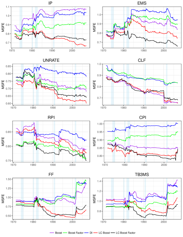
Figure 7: MSFE by start date of out of sample period. Horizon $h=3$. More specifically we plot: $MSFE^{3}_{(i)}(T_{1},T_{2})=\sum_{t=T_{1}}^{T_{2}}\hat{\epsilon}^{2}_{t,(i)}/\sum_{t=T_{1}}^{T_{2}}\hat{\epsilon}^{2}_{t,(AR)}$, where we $T_{1}$ vary from 1971:9 until 2006:12, with $T_{2}$=2018:8. Shaded regions represent NBER recession dates.

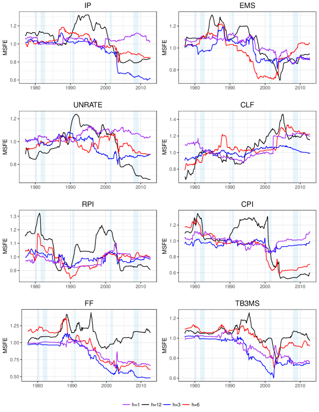
Figure 8: Local MSFE of LC-Boost relative to Local MSFE of Boost: To obtain the local MSFE of a model we use a rolling mean with a window size of 70 observations, which gives us: $\text{L-MSFE}_{i}(t_{0})=\sum_{t=t_{0}-70}^{t_{0}+70}\hat{\epsilon}_{t,(i)}^{2}/\sum_{t=t_{0}-70}^{t_{0}+70}\hat{\epsilon}_{t,(AR)}^{2}$ with the convention that $\hat{\epsilon}_{t,(i)}=0$ for $t\leq 0,t\geq T$. We then plot $\text{L-MSFE}_{LCBoost}(t)/\text{L-MSFE}_{Boost}(t)$, for $t=\text{1977:3},\ldots,\text{2012:10}$

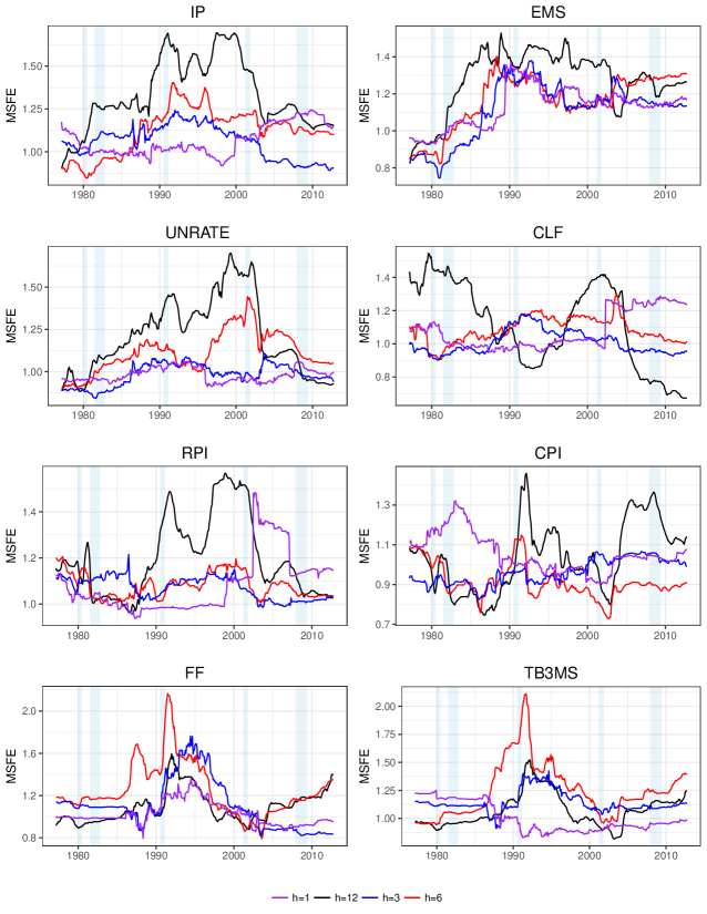
Figure 9: L-MSFE of LC-Boost relative to L-MSFE of LC-Boost Factor: This figure uses a window size of 70 observations to calculate the L-MSFE, see notes to figure 8

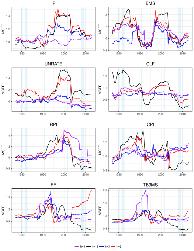
Figure 10: L-MSFE of Boost Factor using 10 year rolling window relative to L-MSFE of LC-Boost Factor: This figure uses a window size of 70 observations to calculate the L-MSFE, see notes to figure 8

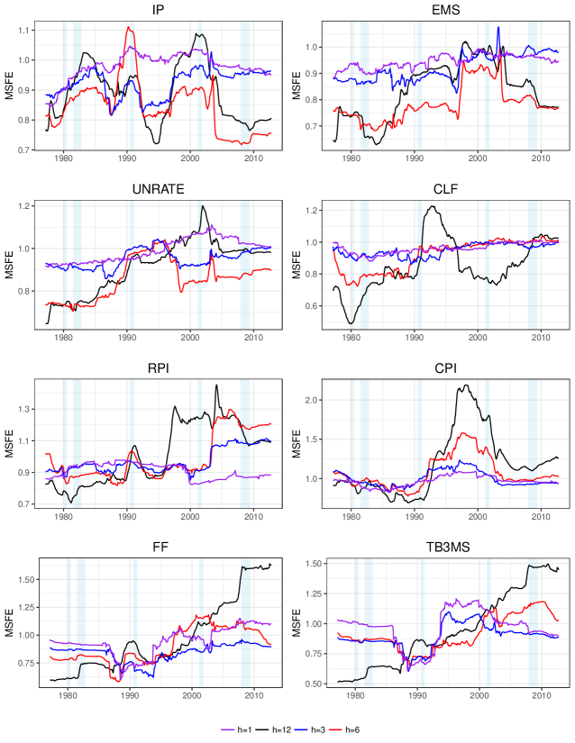
Figure 11: L-MSFE of LC-Boost Factor relative to L-MSFE of LL-Boost Factor: We use a window size of $70$ observations, see notes to figure 8 for details. Colored lines represent the different horizons.

References

- Adrian et al. (2019) Adrian, T., Boyarchenko, N., and Giannone, D. (2019). Vulnerable growth. American Economic Review, 109(4):1263–89.
- Bai and Ng (2002) Bai, J. and Ng, S. (2002). Determining the number of factors in approximate factor models. Econometrica, 70(1):191–221.
- Bai and Ng (2009) Bai, J. and Ng, S. (2009). Boosting diffusion indices. Journal of Applied Econometrics, 24(4):607–629.
- Basu and Michailidis (2015) Basu, S. and Michailidis, G. (2015). Regularized estimation in sparse high-dimensional time series models. Ann. Statist., 43:1535–1567.
- Bates et al. (2013) Bates, B. J., Plagborg-Møller, M., Stock, J. H., and Watson, M. W. (2013). Consistent factor estimation in dynamic factor models with structural instability. Journal of Econometrics, 177(2):289–304.
- Breitung and Eickmeier (2011) Breitung, J. and Eickmeier, S. (2011). Testing for structural breaks in dynamic factor models. Journal of Econometrics, 163(1):71–84.
- Buhlmann (2006) Buhlmann, P. (2006). Boosting for high-dimensional linear models. Ann. Statist., 2(34):559–583.
- Buhlmann and Hothorn (2007) Buhlmann, P. and Hothorn, T. (2007). Boosting algorithms: Regularization, prediction and model fitting. Statistical Science, 22(4):477–505.
- Cai (2007) Cai, Z. (2007). Trending time-varying coefficient time series models with serially correlated errors. Journal of Econometrics, 136(1):163–188.
- Carrasco and Rossi (2016) Carrasco, M. and Rossi, B. (2016). In-sample inference and forecasting in misspecified factor models. Journal of Business & Economic Statistics, 34(3):313–338.
- Carriero et al. (2019) Carriero, A., Clark, T. E., and Marcellino, M. (2019). Large bayesian vector autoregressions with stochastic volatility and non-conjugate priors. Journal of Econometrics.
- Casini and Perron (2018) Casini, A. and Perron, P. (2018). Structural breaks in time series. arXiv preprint arXiv:1805.03807.
- Chan et al. (2012) Chan, J. C., Koop, G., Leon-Gonzalez, R., and Strachan, R. W. (2012). Time varying dimension models. Journal of Business & Economic Statistics, 30(3):358–367.
- Chen (2015) Chen, B. (2015). Modeling and testing smooth structural changes with endogenous regressors. Journal of Econometrics, 185(1):196–215.
- Chen and Hong (2012) Chen, B. and Hong, Y. (2012). Testing for smooth structural changes in time series models via nonparametric regression. Econometrica, 80(3):1157–1183.
- Chen et al. (2013) Chen, X., Xu, M., and Wu, W. B. (2013). Covariance and precision matrix estimation for high-dimensional time series. Ann. Statist., 41:2994–3021.
- Clements and Hendry (1996) Clements, M. P. and Hendry, D. F. (1996). Intercept corrections and structural change. Journal of Applied Econometrics, 11(5):475–494.
- Clements and Hendry (2000) Clements, M. P. and Hendry, D. F. (2000). Forecasting non-stationary economic time series. MIT Press.
- Cogley and Sargent (2001) Cogley, T. and Sargent, T. J. (2001). Evolving post-world war ii US inflation dynamics. NBER macroeconomics annual, 16:331–373.
- Dahlhaus (1996) Dahlhaus, R. (1996). On the kullback-leibler information divergence of locallystationary processes. Stochastic processes and their applications, 62(1):139–168.
- Dahlhaus (2012) Dahlhaus, R. (2012). Locally stationary processes. In Handbook of statistics, volume 30, pages 351–413. Elsevier.
- Dahlhaus et al. (1997) Dahlhaus, R. et al. (1997). Fitting time series models to nonstationary processes. The annals of Statistics, 25(1):1–37.
- Dahlhaus et al. (2018) Dahlhaus, R., Richter, S., and Wu, W. B. (2018). Towards a general theory for non-linear locally stationary processes. Bernoulli. In press.
- Dangl and Halling (2012) Dangl, T. and Halling, M. (2012). Predictive regressions with time-varying coefficients. Journal of Financial Economics, 106(1):157–181.
- Ding et al. (2017) Ding, X., Qiu, Z., Chen, X., et al. (2017). Sparse transition matrix estimation for high-dimensional and locally stationary vector autoregressive models. Electronic Journal of Statistics, 11(2):3871–3902.
- Doukhan (1994) Doukhan, P. (1994). Mixing: Properties and Examples, volume 85 of Lecture Notes in Statistics. Springer-Verlag New York.
- Efron et al. (2004) Efron, B., Hastie, T., Johnstone, I., Tibshirani, R., et al. (2004). Least angle regression. The Annals of statistics, 32(2):407–499.
- Eickmeier et al. (2015) Eickmeier, S., Lemke, W., and Marcellino, M. (2015). Classical time varying factor-augmented vector auto-regressive models—estimation, forecasting and structural analysis. Journal of the Royal Statistical Society: Series A (Statistics in Society), 178(3):493–533.
- Fan et al. (2011) Fan, J., Lv, J., and Qi, L. (2011). Sparse high-dimensional models in economics. Annu. Rev. Econ., 3(1):291–317.
- Fenske et al. (2011) Fenske, N., Kneib, T., and Hothorn, T. (2011). Identifying risk factors for severe childhood malnutrition by boosting additive quantile regression. Journal of the American Statistical Association, 106(494):494–510.
- Freund and Schapire (1997) Freund, Y. and Schapire, R. E. (1997). A decision-theoretic generalization of on-line learning and an application to boosting. Journal of computer and system sciences, 55(1):119–139.
- Friedman et al. (2004) Friedman, J., Hastie, T., Rosset, S., Tibshirani, R., and Zhu, J. (2004). Discussion of boosting papers. Ann. Statist, 32:102–107.
- Friedman et al. (2001) Friedman, J., Hastie, T., and Tibshirani, R. (2001). The elements of statistical learning, volume 1. Springer series in statistics New York, NY, USA:.
- Friedman et al. (2000) Friedman, J., Hastie, T., Tibshirani, R., et al. (2000). Additive logistic regression: a statistical view of boosting (with discussion and a rejoinder by the authors). The annals of statistics, 28(2):337–407.
- Friedman (2001) Friedman, J. H. (2001). Greedy function approximation: a gradient boosting machine. Annals of statistics, pages 1189–1232.
- Fryzlewicz et al. (2011) Fryzlewicz, P., Rao, S. S., et al. (2011). Mixing properties of arch and time-varying arch processes. Bernoulli, 17(1):320–346.
- Giraitis et al. (2013) Giraitis, L., Kapetanios, G., and Price, S. (2013). Adaptive forecasting in the presence of recent and ongoing structural change. Journal of Econometrics, 177(2):153–170.
- Goyal and Welch (2003) Goyal, A. and Welch, I. (2003). Predicting the equity premium with dividend ratios. Management Science, 49(5):639–654.
- Groen et al. (2013) Groen, J. J., Paap, R., and Ravazzolo, F. (2013). Real-time inflation forecasting in a changing world. Journal of Business & Economic Statistics, 31(1):29–44.
- Hamilton (1989) Hamilton, J. D. (1989). A new approach to the economic analysis of nonstationary time series and the business cycle. Econometrica: Journal of the Econometric Society, pages 357–384.
- Han and Tsay (2017) Han, Y. and Tsay, R. S. (2017). High-dimensional linear regression for dependent observations with application to nowcasting. arXiv preprint arXiv:1706.07899.
- Hastie et al. (2007) Hastie, T., Taylor, J., Tibshirani, R., and Walther, G. (2007). Forward stagewise regression and the monotone lasso. Electronic Journal of Statistics, 1:1–29.
- Hepp et al. (2016) Hepp, T., Schmid, M., Gefeller, O., Waldmann, E., and Mayr, A. (2016). Approaches to regularized regression–a comparison between gradient boosting and the lasso. Methods of information in medicine, 55(05):422–430.
- Hofner et al. (2014) Hofner, B., Mayr, A., Robinzonov, N., and Schmid, M. (2014). Model-based boosting in r: a hands-on tutorial using the r package mboost. Computational statistics, 29(1-2):3–35.
- Hörmann et al. (2010) Hörmann, S., Kokoszka, P., et al. (2010). Weakly dependent functional data. The Annals of Statistics, 38(3):1845–1884.
- Hu et al. (2018) Hu, L., Huang, T., and You, J. (2018). Estimation and identification of a varying-coefficient additive model for locally stationary processes. Journal of the American Statistical Association. In Press.
- Inoue et al. (2017) Inoue, A., Jin, L., and Rossi, B. (2017). Rolling window selection for out-of-sample forecasting with time-varying parameters. Journal of Econometrics, 196(1):55–67.
- Kelly and Pruitt (2015) Kelly, B. and Pruitt, S. (2015). The three-pass regression filter: A new approach to forecasting using many predictors. Journal of Econometrics, 186(2):294 – 316. High Dimensional Problems in Econometrics.
- Kim and Swanson (2014) Kim, H. H. and Swanson, N. R. (2014). Forecasting financial and macroeconomic variables using data reduction methods: New empirical evidence. Journal of Econometrics, 178:352–367.
- Kock and Callot (2015) Kock, A. and Callot, A. (2015). Oracle inequalities for high dimensional vector autoregressions. Journal of Econometrics, 186:325 – 344.
- Koop and Korobilis (2012) Koop, G. and Korobilis, D. (2012). Forecasting inflation using dynamic model averaging. International Economic Review, 53(3):867–886.
- Koop and Korobilis (2013) Koop, G. and Korobilis, D. (2013). Large time-varying parameter vars. Journal of Econometrics, 177(2):185–198.
- Koop (2013) Koop, G. M. (2013). Forecasting with medium and large bayesian vars. Journal of Applied Econometrics, 28(2):177–203.
- Lee et al. (2016) Lee, E. R., Mammen, E., et al. (2016). Local linear smoothing for sparse high dimensional varying coefficient models. Electronic Journal of Statistics, 10(1):855–894.
- Lutz and Bühlmann (2006) Lutz, R. W. and Bühlmann, P. (2006). Boosting for high-multivariate responses in high-dimensional linear regression. Statistica Sinica, 16(2):471–494.
- McCracken and Ng (2016) McCracken, M. W. and Ng, S. (2016). FRED-MD: A monthly database for macroeconomic research. Journal of Business & Economic Statistics, 34(4):574–589.
- McDonald et al. (2015) McDonald, D. J., Shalizi, C. R., and Schervish, M. (2015). Estimating beta-mixing coefficients via histograms. Electronic Journal of Statistics, 9(2):2855–2883.
- Medeiros and Mendes (2016) Medeiros, M. and Mendes, E. (2016). 1-regularization of high-dimensional time-series models with non-gaussian and heteroskedastic errors. Journal of Econometrics, 191:255–271.
- Ng (2013) Ng, S. (2013). Variable selection in predictive regressions. In Elliott, G. and Timmermann, A., editors, Handbook of Forecasting, number 754-786 in 2B. North Holland.
- Ng (2014) Ng, S. (2014). Viewpoint: Boosting recessions. Canadian Journal of Economics/Revue canadienne d’économique, 47(1):1–34.
- Orbe et al. (2005) Orbe, S., Ferreira, E., and Rodriguez-Poo, J. (2005). Nonparametric estimation of time varying parameters under shape restrictions. Journal of Econometrics, 126(1):53–77.
- Orbe et al. (2006) Orbe, S., Ferreira, E., and Rodriguez-Poo, J. (2006). On the estimation and testing of time varying constraints in econometric models. Statistica Sinica, pages 1313–1333.
- Paye and Timmermann (2006) Paye, B. S. and Timmermann, A. (2006). Instability of return prediction models. Journal of Empirical Finance, 13(3):274–315.
- Perron et al. (2006) Perron, P. et al. (2006). Dealing with structural breaks. Palgrave handbook of econometrics, 1(2):278–352.
- Pesaran and Timmermann (2007) Pesaran, M. H. and Timmermann, A. (2007). Selection of estimation window in the presence of breaks. Journal of Econometrics, 137(1):134–161.
- Petrova (2019) Petrova, K. (2019). A quasi-bayesian local likelihood approach to time varying parameter var models. Journal of Econometrics.
- Pettenuzzo and Timmermann (2017) Pettenuzzo, D. and Timmermann, A. (2017). Forecasting macroeconomic variables under model instability. Journal of Business & Economic Statistics, 35(2):183–201.
- Phillips et al. (2017) Phillips, P. C., Li, D., and Gao, J. (2017). Estimating smooth structural change in cointegration models. Journal of Econometrics, 196(1):180–195.
- Primiceri (2005) Primiceri, G. E. (2005). Time varying structural vector autoregressions and monetary policy. The Review of Economic Studies, 72(3):821–852.
- Rapach et al. (2010) Rapach, D. E., Strauss, J. K., and Zhou, G. (2010). Out-of-sample equity premium prediction: Combination forecasts and links to the real economy. The Review of Financial Studies, 23(2):821–862.
- Richter and Dahlhaus (2018) Richter, S. and Dahlhaus, R. (2018). Cross validation for locally stationary processes. Ann. Statist. In Press.
- Robinson (1989) Robinson, P. M. (1989). Nonparametric estimation of time-varying parameters. In Statistical Analysis and Forecasting of Economic Structural Change, pages 253–264. Springer.
- Robinson (1991) Robinson, P. M. (1991). Time-varying nonlinear regression. In Economic Structural Change, pages 179–190. Springer.
- Rosset et al. (2004) Rosset, S., Zhu, J., and Hastie, T. (2004). Boosting as a regularized path to a maximum margin classifier. Journal of Machine Learning Research, 5(Aug):941–973.
- Rossi (2013) Rossi, B. (2013). Advances in forecasting under instability. In Handbook of economic forecasting, volume 2, pages 1203–1324. Elsevier.
- Rossi and Sekhposyan (2010) Rossi, B. and Sekhposyan, T. (2010). Have economic models’ forecasting performance for US output growth and inflation changed over time, and when? International Journal of Forecasting, 26(4):808–835.
- Schinasi and Swamy (1989) Schinasi, G. J. and Swamy, P. A. V. B. (1989). The out-of-sample forecasting performance of exchange rate models when coefficients are allowed to change. Journal of International Money and Finance, 8(3):375–390.
- Shapiro (2017) Shapiro, J. M. (2017). Is Big Data a Big Deal for Applied Microeconomics?, volume 2 of Econometric Society Monographs, page 35–52. Cambridge University Press.
- Stock and Watson (2003) Stock, J. H. and Watson, M. (2003). Forecasting output and inflation: The role of asset prices. Journal of Economic Literature, 41(3):788–829.
- Stock and Watson (2009) Stock, J. H. and Watson, M. (2009). Forecasting in dynamic factor models subject to structural instability. The Methodology and Practice of Econometrics. A Festschrift in Honour of David F. Hendry, 173:205.
- Stock and Watson (1996) Stock, J. H. and Watson, M. W. (1996). Evidence on structural instability in macroeconomic time series relations. Journal of Business & Economic Statistics, 14(1):11–30.
- Stock and Watson (2002) Stock, J. H. and Watson, M. W. (2002). Has the business cycle changed and why? NBER Macroeconomics Annual, 17:159–218.
- Temlyakov (2000) Temlyakov, V. N. (2000). Weak greedy algorithms. Advances in Computational Mathematics, 12(2-3):213–227.
- Terasvirta (1994) Terasvirta, T. (1994). Specification, estimation, and evaluation of smooth transition autoregressive models. Journal of the American Statistical Assocation, 89(425):208–218.
- Vogt et al. (2012) Vogt, M. et al. (2012). Nonparametric regression for locally stationary time series. The Annals of Statistics, 40(5):2601–2633.
- Wu and Wu (2016) Wu, W. and Wu, Y. (2016). Performance bounds for parameter estimates of high-dimensional linear models with correlated errors. Electronic Journal of Statistics, 10:352–379.
- Wu (2005) Wu, W. B. (2005). Nonlinear system theory: Another look at dependence. Proceedings of the National Academy of Sciences, 102(40):14150–14154.
- Wu (2011) Wu, W. B. (2011). Asymptotic theory for stationary processes . Statistics and its Interface, 4(2):207–226.
- Yousuf (2018) Yousuf, K. (2018). Variable screening for high dimensional time series. Electronic Journal of Statistics, 12(1):667–702.
- Zhang et al. (2015) Zhang, T., Wu, W. B., et al. (2015). Time-varying nonlinear regression models: Nonparametric estimation and model selection. The Annals of Statistics, 43(2):741–768.
- Zhou (2010) Zhou, Z. (2010). Nonparametric inference of quantile curves for nonstationary time series. The Annals of Statistics, 38(4):2187–2217.
- Zhou and Wu (2009) Zhou, Z. and Wu, W. B. (2009). Local linear quantile estimation for nonstationary time series. The Annals of Statistics, 37(5B):2696–2729.