Error Probability Analysis and Power Allocation for Interference Exploitation Over Rayleigh Fading Channels

Abstract

This paper considers the performance analysis of constructive interference (CI) precoding technique in multi-user multiple-input multiple-output (MU-MIMO) systems with a finite constellation phase-shift keying (PSK) input alphabet. Firstly, analytical expressions for the moment generating function (MGF) and the average of the received signal-to-noise-ratio (SNR) are derived. Then, based on the derived MGF expression the average symbol error probability (SEP) for the CI precoder with PSK signaling is calculated. In this regard, new exact and very accurate asymptotic approximation for the average SEP are provided. Building on the new performance analysis, different power allocation schemes are considered to enhance the achieved SEP. In the first scheme, power allocation based on minimizing the sum symbol error probabilities (Min-Sum) is studied, while in the second scheme the power allocation based on minimizing the maximum SEP (Min-Max) is investigated. Furthermore, new analytical expressions of the throughput and power efficiency of the CI precoding in MU-MIMO systems are also derived. The numerical results in this work demonstrate that, the CI precoding outperforms the conventional interference suppression precoding techniques with an up to 20dB gain in the transmit SNR in terms of SEP, and up to 15dB gain in the transmit SNR in terms of the throughput. In addition, the SEP-based power allocation schemes provide additional up to 13dB gains in the transmit SNR compared to the conventional equal power allocation scheme.

I Introduction

Multi-user multiple-input multiple-output (MU-MIMO) communication system has been recognized as a promising technique in wireless communication networks [2, 3, 4]. However, in practical implementations the performance of MU-MIMO systems can be impacted by strong interferences [2, 3, 4]. Consequently, a large number of researches have investigated the impact of the interference in MU-MIMO systems, and several techniques have been introduced to mitigate the multi-user interference in MU-MIMO channels [4, 5, 6]. For instance, in the applications when the channel state information (CSI) is perfectly known at the base station (BS), dirty-paper coding (DPC) technique has been proposed [7, 8, 9, 10]. In DPC technique the channel capacity is achieved by removing the interference before the transmission. However, DPC is difficult if not impossible to implement in practical communication networks, due to its very high complexity [7, 8, 9, 10]. Therefore, low complexity linear precoding techniques, such as zero-forcing (ZF), have received significant research interest [11, 12]. Furthermore, precoding techniques based on optimization have also widely studied and investigated in literature [13, 14, 15, 16]. In this regard, several optimization-based schemes have been proposed in different areas. For instance, signal-to-interference-plus-noise ratio (SINR) balancing technique is one of these precoding schemes that depends on maximizing the minimum SINR subject to different transmission power constraints [13, 14]. In addition, minimizing the transmission power precoding is another precoding scheme that aims to minimize the transmission power subject to a minimum threshold value of the SINR [15, 16].

However, all the above precoding/transmission schemes have ignored the fact that the interference in communication systems can be beneficial to the received signal, and thus the multi-user interference can be exploited to further enhance the system performance. In light of this, constructive interference (CI) precoding technique has been proposed recently to improve the performance of down-link MIMO systems [17, 18, 19, 20, 21]. In contrast to the conventional interference mitigation techniques, the main idea of the CI precoding scheme is to exploit the interference that can be known to the BS/transmitter to enhance the received power of the useful signals[17, 18, 19, 20, 21]. That is, with the knowledge of both the users’ channels and users’ data symbols, the BS can classify the interference as constructive and destructive. The constructive interference is the interference that can push the received symbol deeper in the constructive/detection region of the constellation point of interest. According to this methodology, the preceder can be designed to make all the well known interferences constructive to the desired symbol. The main idea of CI precoding for PSK constellations is clarified in [19, Section-III].

The concept of interference exploitation technique has been widely considered in literature. This line of research was introduced in [17], where the CI precoding technique has been proposed for downlink MIMO systems. In this work it was shown that by exploiting the interference signals, the system performance can be greatly enhanced and the effective SINR can be improved without increasing the transmission power at the BS. In [18] the concept of CI was used for the first time to design an optimization-based precoder in the form of pre-scaling. In [19] the authors proposed CI-based precoding schemes for down-link MU-MIMO systems to minimize the transmit power for generic PSK signals. The concept of CI was applied to massive-MIMO systems in [20]. Further work in [21, 22] implemented CI precoding scheme in wireless power transfer scenarios for PSK messages, in order to minimize the total transmit power. The authors in [23, 24] considered general category of CI regions, named distance preserving CI region, where several properties for this region have been provided. Furthermore, recently closed-form expression for CI precoding technique in MU-MIMO systems with PSK signaling has been derived in [10]. This closed-form expression has paved the way to develop theoretical analysis of the CI technique. Based on this closed-form expression for CI precoding, in our previous work in [25, 26] closed-form expression of the achievable sum-rate of the CI precoding technique in MU-MIMO systems has been derived and investigated.

Accordingly this paper is the first work characterizes the statistics of CI precoding with $M$-PSK signals in MU-MIMO systems. Firstly, analytical expressions of the moment-generating function (MGF) and the average of the received SNR of the considered system are derived. The derived MGF expression is then used to evaluate the average symbol error probability (SEP). In this regard, exact SEP expression for CI precoding with $M$-PSK signals is derived. For simplicity and in order to provide more insight, very accurate asymptotic approximation for the SEP is also presented. Based on the new SEP expressions, different power allocation schemes to enhance the achieved SEP are considered. In the first one, power allocation technique that based on minimizing the sum symbol error probabilities (Min-Sum) is studied, while in the second technique the power allocation that based on minimizing the average SEP (Min-MAx) is investigated. Furthermore, the throughput and power efficiency achieved by the CI precoding in MU-MIMO systems are also studied. In this context, new analytical expressions of the throughput and power efficiency are provided.

For clarity, we summarize the main contributions of this paper as:

1. New and explicit analytical expressions for the MGF and the average of the received SNR for CI precoding technique under $M$-PSK inputs are derived.

2. New, exact, and explicit expression of the average SEP for CI precoding with $M$-PSK is derived. For simplicity and mathematical tractability, new and very accurate asymptotic approximation of the SEP is also provided.

3. Two power allocation schemes to improve the SEP and enhance the system performance are proposed. In the first one, we consider power allocation technique that aims to minimize the sum symbol error probabilities subject to total power constraint. Whilst in the second scheme, we study power allocation technique that aims to minimize the maximum SEP subject to total power constraint.

4. Based on the above analysis, closed form expression of the power allocation factors are presented.

5. New and explicit analytical expressions for the throughput and power efficiency for the CI precoding in MU-MIMO systems under $M$-PSK inputs are also derived.

The numerical results in this paper show that, for a given SEP the CI precoding can provide up to 20dB gain in the transmit SNR compared to the conventional interference suppression precoding techniques. In addition, increasing the transmit SNR, number of users and number of BS antennas always enhance the achieved SEP. Furthermore, by using the derived analysis specifically tailored power allocation schemes provide additional up to 13dB gains in the transmit SNR compared to the conventional transmission scheme. Finally, the CI precoding outperforms the conventional interference suppression precoding technique in terms of throughput for a wide range with an up to 15dB gain in the transmit SNR.

Next, Section II describes the MU-MIMO system model. Section III, derives the analytical expressions for the moment generating function and the average received SNR. Section IV derives the exact and approximated analytical expressions for the average symbol error probability. Section V, considers symbol error minimization through different power allocation schemes, minimizing the sum symbol error probabilities and minimizing the maximum symbol error probability. Section VI, considers the throughput and power efficiency for the CI precoding in MU-MIMO systems. The graphical illustrations of the results are presented and discussed in Section VII. Finally, our conclusions are presented in Section VIII.

II System Model

We consider a down-link MU-MIMO system, consisting of $N$-antennas BS communicating simultaneously with $K$ single antenna users. In this model, the channels between the BS and the users are assumed to be independent identically distributed (i.i.d) Rayleigh fading channels. The $K\times N$ channel matrix between the BS and the $K$ users is denoted by $\mathbf{H}$, which can be expressed as $\mathbf{H}=\mathbf{D}^{1/2}\tilde{\mathbf{H}}$ where $\tilde{\mathbf{H}}$ is $K\times N$ matrix has i.i.d $\mathcal{CN}\left(\text{0,}1\right)$ elements which represent small scale fading coefficients and $\mathbf{D}$ is $K\times K$ a diagonal matrix with$\left[\mathbf{D}\right]_{kk}=\varpi_{k}=d_{k}^{-m}$ and $m$ is the path-loss exponent, which represents the path-loss attenuation. It is also assumed that the CSI is perfectly known at the BS. The received signal at the $k^{th}$ user in the considered system can be written as,

$$y_{k}=\mathbf{h}_{k}\mathbf{W}\mathbf{x}+n_{k}$$ (1)

where $\mathbf{x}$ is the PSK-modulated signal vector, $\mathbf{W}$ is the precoding matrix, $\mathbf{h}_{k}$ is the channel vector of user $k$, and $n_{k}$ is the additive wight Gaussian noise (AWGN) at the $k^{th}$ user, $n_{k}\sim\mathcal{CN}\left(\text{0, }\sigma_{k}^{2}\right)$. The closed-form expression for CI precoding with PSK signaling can be expressed as [10, 25, 26]

$$\mathbf{W}=\frac{1}{K}\beta\,\mathbf{H}^{H}\left(\mathbf{H}\mathbf{H}^{H}\right)^{-1}\textrm{diag}\left\{\mathbf{V}^{-1}\mathbf{u}\right\}\mathbf{x}\mathbf{x}^{H},$$ (2)

where $\beta=\sqrt{P_{p}}\beta_{p}$, $P_{p}$ is the total transmit power and $\beta_{P}$ is the scaling factor, $\beta_{p}=\sqrt{\frac{1}{\mathbf{u}^{H}\mathbf{V}^{-1}\mathbf{u}}}$, while $\mathbf{V}=\textrm{diag}\left(\mathbf{x}^{H}\right)\left(\mathbf{H}\mathbf{H}^{H}\right)^{-1}\textrm{diag}\left(\mathbf{x}\right)$ and $\mathbf{1}^{H}\mathbf{u}=1$. As by CI precoding the resulting interference contributes to the useful signal power, it has been shown that the received SNR at user $k$ using CI precoding technique can be written as [19, 22]

$$\gamma_{k}=\frac{\left|\boldsymbol{h}_{k}\mathbf{W}\mathbf{x}\right|^{2}}{\sigma_{k}^{2}}$$ (3)

In the following sections we will study the statistics of the received SNR and analyze the performance of CI precoding technique in details.

III MGF and Average SNR for CI Precoding

In this section, we derive the MGF and the average SNR expressions of the considered MU-MIMO system. To start with, by substituting (2) into (3), the SNR at user $k$ using CI precoding technique can be expressed as

$$\gamma_{k}=\frac{\left|\boldsymbol{h}_{k}\frac{\sqrt{P_{p}}\beta_{p}}{K}\,\mathbf{H}^{H}\left(\mathbf{H}\mathbf{H}^{H}\right)^{-1}\textrm{diag}\left\{\mathbf{V}^{-1}\mathbf{u}\right\}\mathbf{x}\right|^{2}}{\sigma_{k}^{2}}$$ (4)

For simplicity but without loss of generality, the scaling factor $\beta_{p}$ is designed to constrain the long-term total transmit power at the BS, and thus it can be expressed as [5, 10] $\beta_{p}=\frac{1}{\sqrt{\mathcal{E}\left\{\mathbf{u}^{H}\mathbf{V}^{-1}\mathbf{u}\right\}}}$. Since $\left(\mathbf{H}\mathbf{H}^{H}\right)$ has Wishart distribution, we can find that, $\beta_{p}=\frac{1}{\sqrt{\mathbf{u}^{H}\textrm{diag}\left(\mathbf{x}^{H}\right)^{-1}\,N\mathbf{\Sigma}\left(\textrm{diag}\left(\mathbf{x}\right)\right)^{-1}\mathbf{u}}}$, where $\Sigma=\textrm{D}$ [27]. The last formula in (4) can be expressed also as

$$\gamma_{k}=\frac{\left|\frac{\sqrt{P_{p}}\beta_{p}}{K}\boldsymbol{b}\mathbf{A}\mathbf{u}x_{k}\right|^{2}}{\sigma_{k}^{2}}$$ (5)

where $\mathbf{b}=\mathbf{a}_{k}$ , $\mathbf{a}_{k}$ is a $1\times K$ vector the $k^{th}$ element of this vector is one and all the other elements are zeros, and $\mathbf{A}=\mathbf{V}^{-1}$. We can re-write the SNR expression in (5) as

$$\gamma_{k}=\frac{\left|\frac{\sqrt{P_{p}}\beta_{p}}{K}\mathbf{b}\Sigma\mathbf{u}\frac{\boldsymbol{b}\mathbf{A}\mathbf{u}}{\mathbf{b}\Sigma\mathbf{u}}x_{k}\right|^{2}}{\sigma_{k}^{2}}=\alpha_{k}\left|g\right|^{2}$$ (6)

where $\alpha_{k}=\frac{\left|\frac{\sqrt{P_{p}}\beta_{p}}{K}\mathbf{b}\Sigma\mathbf{u}\right|^{2}}{\sigma_{k}^{2}}$ and $g=\frac{\boldsymbol{b}\mathbf{A}\mathbf{u}}{\mathbf{b}\Sigma\mathbf{u}}$. It was shown in literature that, the distribution of $g=\frac{\boldsymbol{b}\mathbf{A}\mathbf{u}}{\mathbf{b}\Sigma\mathbf{u}}$ can be approximated to Gamma distribution with shape parameter $\nu$ and scale parameter $\theta$, $g\thicksim\Gamma\left(\nu,\theta\right)$ [27, 28]. Consequently, the received SNR, $\gamma_{k}$, can be approximated to General Gamma distribution $\Gamma\left(p,d,a\right)$ with $p=\frac{1}{2}$, $d=\frac{\nu}{2}$ and $a=\theta^{2}$. Therefore, the cumulative distribution function (CDF) and the probability density function (PDF) of the received SNR, $\gamma_{k}$, can be written, respectively, as

$$F_{\gamma_{k}}\left(\gamma\right)=\left(\frac{\varphi\left(d/p,\left(\gamma/a\right)^{p}\right)}{\Gamma\left(d/p\right)}\right)\;\textrm{and}\;f_{\gamma_{k}}\left(\gamma\right)=\left(\frac{\left(\frac{p}{a^{d}}\right)\gamma^{d-1}e^{-\left(\frac{\gamma}{a}\right)^{p}}}{\Gamma\left(\frac{d}{p}\right)}\right)$$ (7)

where $\varphi\left(.\right)$ is the lower incomplete Gamma function. Now the MGF of the received SNR, $\gamma_{k}$, can be derived as

$$\mathcal{M}_{\gamma_{k}}\left(z\right)=\stackrel{{\scriptstyle[}}{{0}}]{\infty}{\int}e^{-z\gamma}f_{\gamma_{k}}\left(\gamma\right)d\gamma$$ (8)

Substituting the PDF in (7) into (8), we can find

$$\mathcal{M}_{\gamma}\left(z\right)=\stackrel{{\scriptstyle[}}{{0}}]{\infty}{\int}e^{-z\gamma}\left(\frac{\left(\frac{p}{a^{d}}\right)\gamma^{d-1}e^{-\left(\frac{\gamma}{a}\right)^{p}}}{\Gamma\left(\frac{d}{p}\right)}\right)d\gamma$$ (9)

Applying Gaussian Quadrature rule, the MGF can be simplified to

$$\mathcal{M}_{\gamma}\left(z\right)=\stackrel{{\scriptstyle[}}{{i}}=1]{n}{\sum}\textrm{H}_{i}\left(\frac{\left(\frac{p}{a^{d}}\right)e^{-\left(z-1\right)\gamma_{i}}\left(\gamma_{i}\right)^{d-1}e^{-\left(\frac{\gamma_{i}}{a}\right)^{p}}}{\Gamma\left(\frac{d}{p}\right)}\right)$$ (10)

where $\gamma_{i}$ and $\textrm{H}_{i}$ are the $i^{th}$ zero and the weighting factor of the Laguerre polynomials, respectively [29]. Alternatively, using Gamma distribution we can find

$$\mathcal{M}_{\gamma}\left(z\right)=\stackrel{{\scriptstyle[}}{{i}}=1]{n}{\sum}\textrm{H}_{i}e^{-zP_{p}\zeta_{k}\left|g_{i}\right|^{2}}\left(\frac{g_{i}^{N-1}}{\left(N-1\right)!}\right)$$ (11)

where $\zeta_{k}=\frac{\left|\frac{\beta_{p}}{K}\mathbf{b}\Sigma\mathbf{u}\right|^{2}}{\sigma_{k}^{2}}$, $g_{i}$ here is the $i^{th}$ zero of the Laguerre polynomials [29].

III-A Average SNR

The average SNR of CI precoder can be obtained from the first derivative of $\mathcal{M}_{\gamma}\left(z\right)$ expressions evaluated at $z=0$. Hence, the average SNR can be calculated by

$$\bar{\gamma}_{k}=\left.\frac{\partial\mathcal{M}_{\gamma}\left(z\right)}{\partial z}\right|_{z=0}$$ (12)

$$\bar{\gamma}_{k}=\stackrel{{\scriptstyle[}}{{i}}=1]{n}{\sum}\textrm{H}_{i}\frac{\partial}{\partial z}\left.\left(\frac{\left(\frac{p}{a^{d}}\right)e^{-\left(z-1\right)\gamma_{i}}\left(\gamma_{i}\right)^{d-1}e^{-\left(\frac{\gamma_{i}}{a}\right)^{p}}}{\Gamma\left(\frac{d}{p}\right)}\right)\right|_{z=0}$$ (13)

Using a standard approach, the average of the SNR can be expressed as

$$\bar{\gamma}_{k}=\stackrel{{\scriptstyle[}}{{0}}]{\infty}{\int}\gamma\,f_{\gamma_{k}}\left(\gamma\right)d\gamma$$ (14)

Substituting the PDF in (7) into (14) we can get,

$$\bar{\gamma}_{k}=\left(\frac{a\Gamma\left(\frac{1+d}{p}\right)}{\Gamma\left(\frac{d}{p}\right)}\right)=\frac{\alpha_{k}^{2}\Gamma\left(N+2\right)}{\Gamma\left(N\right)}$$ (15)

IV Average Symbol Error Probability (SEP)

In this section we calculate the average SEP for CI precoding with $M$-PSK signaling using a standard approach provided in literature [30, 31, (5.67)]. The average SEP of $M$-PSK can be calculated by [30, (5.67)]

$$P_{e,k}=\frac{1}{\pi}\stackrel{{\scriptstyle[}}{{0}}]{\frac{\pi\left(M-1\right)}{M}}{\int}\mathcal{M}_{\gamma}\left(-\frac{\sin^{2}\left(\frac{\pi}{M}\right)}{\sin^{2}\Phi}\right)d\Phi$$ (16)

Next we will provide exact and approximated formulas to calculate the average SEP for MU-MIMO transmission using CI precoding technique.

IV-A Exact SEP

For simplicity (16) can be written as

$$P_{e,k}=\frac{1}{\pi}\stackrel{{\scriptstyle[}}{{0}}]{\Theta}{\int}\mathcal{M}_{\gamma}\left(z\right)d\theta$$ (17)

where $\Theta=\frac{\pi\left(M-1\right)}{M}$ and $z=-\frac{\sin^{2}\left(\frac{\pi}{M}\right)}{\sin^{2}\Phi}$. By Substituting (10) into (17), we can get

$$P_{e,k}=\frac{1}{\pi}\stackrel{{\scriptstyle[}}{{i}}=1]{n}{\sum}\stackrel{{\scriptstyle[}}{{0}}]{\Theta}{\int}\frac{\textrm{H}_{i}}{zP_{p}\zeta_{k}}\left(\frac{\left(\frac{p}{a^{d}}\right)\left(\frac{\upsilon_{i}}{zP_{p}\zeta_{k}}\right)^{d-1}e^{-\left(\frac{\upsilon_{i}}{azP_{p}\zeta_{k}}\right)^{p}}}{\Gamma\left(\frac{d}{p}\right)}\right)d\Phi$$ (18)

and

$$P_{e,k}=\frac{1}{\pi}\stackrel{{\scriptstyle[}}{{i}}=1]{n}{\sum}\stackrel{{\scriptstyle[}}{{0}}]{\Theta}{\int}\textrm{H}_{i}\frac{\left(\frac{p}{a^{d}}\right)\left(\upsilon_{i}\right)^{d-1}e^{-\left(\frac{\upsilon_{i}}{azP_{p}\zeta_{k}}\right)^{p}}}{\left(zP_{p}\zeta_{k}\right)^{d}\Gamma\left(\frac{d}{p}\right)}d\Phi$$ (19)

Using Gamma distribution we can also find

$$P_{e,k}=\frac{1}{\pi}\stackrel{{\scriptstyle[}}{{i}}=1]{n}{\sum}\stackrel{{\scriptstyle[}}{{0}}]{\Theta}{\int}\textrm{H}_{i}e^{-zP_{p}\zeta_{k}\left|g_{i}\right|^{2}}\left(\frac{g_{i}^{N-1}}{\left(N-1\right)!}\right)d\Phi$$ (20)

As we can notice from the derived SEP equations, the derived SEP expressions are represented only with single integration which can be approximated efficiently using numerical integration methods. In order to provide more insights, in the next sub-section we derive an approximation of the average SEP, which is shown in the numerical results to be very accurate.

IV-B Approximate SEP

Here we derive an approximation expression of the average SEP of the considered scenario. Firstly, (17) can be written as

$$P_{e,k}=\mathcal{E}\left[\frac{1}{\pi}\stackrel{{\scriptstyle[}}{{0}}]{\frac{\pi}{2}}{\int}\exp\left(-\frac{\sin^{2}\left(\frac{\pi}{M}\right)}{\sin^{2}\theta}\right)d\theta\right.\left.+\frac{1}{\pi}\stackrel{{\scriptstyle[}}{{\frac{}}{missing}}{\pi}{2}]{\Theta}{\int}\exp\left(-\frac{\sin^{2}\left(\frac{\pi}{M}\right)}{\sin^{2}\theta}\right)d\theta\right]$$ (21)

Now, the first term in (21) can be approximated by [31, 32]

$$\frac{1}{\pi}\stackrel{{\scriptstyle[}}{{0}}]{\frac{\pi}{2}}{\int}\exp\left(-\frac{\sin^{2}\left(\frac{\pi}{M}\right)}{\sin^{2}\theta}\right)d\theta\approx\frac{1}{12}e^{\left(-\sin^{2}\left(\frac{\pi}{M}\right)\right)}+\frac{1}{4}e^{\left(-\frac{4\sin^{2}\left(\frac{\pi}{M}\right)}{3}\right)}$$ (22)

Similarly, the second term in (21) can be approximated as [31, 32]

$$\frac{1}{\pi}\stackrel{{\scriptstyle[}}{{\frac{}}{missing}}{\pi}{2}]{\Theta}{\int}\exp\left(-\frac{\sin^{2}\left(\frac{\pi}{M}\right)}{\sin^{2}\theta}\right)d\theta\approx\frac{1}{2\pi}\left(e^{\left(-\sin^{2}\left(\frac{\pi}{M}\right)\right)}+\frac{1}{4}e^{\left(-\frac{\sin^{2}\left(\frac{\pi}{M}\right)}{\sin^{2}\Theta}\right)}\right)\left(\Theta-\frac{\pi}{2}\right)$$ (23)

Now substituting (22) and (23) into (21), we can obtain approximated expression of SEP as [31, 32]

$$P_{e,k}=\mathcal{E}\left[\frac{1}{12}e^{\left(-\sin^{2}\left(\frac{\pi}{M}\right)\right)}+\frac{1}{4}e^{\left(-\frac{4\sin^{2}\left(\frac{\pi}{M}\right)}{3}\right)}+\frac{1}{2\pi}\left(e^{\left(-\sin^{2}\left(\frac{\pi}{M}\right)\right)}+\frac{1}{4}e^{\left(-\frac{\sin^{2}\left(\frac{\pi}{M}\right)}{\sin^{2}\Theta}\right)}\right)\left(\Theta-\frac{\pi}{2}\right)\right]$$ (24)

which can be written as

$$P_{e,k}=\frac{1}{12}\mathcal{M}_{\gamma}\left(\sin^{2}\left(\frac{\pi}{M}\right)\right)+\frac{1}{4}\mathcal{M}_{\gamma}\left(\frac{4\sin^{2}\left(\frac{\pi}{M}\right)}{3}\right)$$

$$+\frac{1}{2\pi}\left(\mathcal{M}_{\gamma}\left(\sin^{2}\left(\frac{\pi}{M}\right)\right)+\frac{1}{4}\mathcal{M}_{\gamma}\left(\frac{\sin^{2}\left(\frac{\pi}{M}\right)}{\sin^{2}\Theta}\right)\right)\left(\Theta-\frac{\pi}{2}\right)$$ (25)

and

$$P_{e,k}=\left(\frac{\Theta}{2\pi}-\frac{1}{6}\right)\mathcal{M}_{\gamma}\left(\sin^{2}\left(\frac{\pi}{M}\right)\right)+\frac{1}{4}\mathcal{M}_{\gamma}\left(\frac{4\sin^{2}\left(\frac{\pi}{M}\right)}{3}\right)+\left(\frac{\Theta}{2\pi}-\frac{1}{4}\right)\mathcal{M}_{\gamma}\left(\frac{\sin^{2}\left(\frac{\pi}{M}\right)}{\sin^{2}\Theta}\right)$$ (26)

Finally using the derived formula in (26), the approximated expression of the average SEP for MU-MIMO system using CI precoding technique can be written as,

$$P_{e,k}=\left(\frac{\Theta}{2\pi}-\frac{1}{6}\right)\stackrel{{\scriptstyle[}}{{i}}=1]{n}{\sum}\frac{\textrm{H}_{i}}{\sin^{2}\left(\frac{\pi}{M}\right)P_{p}\zeta_{k}}\left(\frac{\left(\frac{p}{a^{d}}\right)\left(\frac{\gamma_{i}}{\sin^{2}\left(\frac{\pi}{M}\right)P_{p}\zeta_{k}}\right)^{d-1}e^{-\left(\frac{\gamma_{i}}{azP_{p}\zeta_{k}}\right)^{p}}}{\Gamma\left(\frac{d}{p}\right)}\right)$$

$$+\frac{1}{4}\stackrel{{\scriptstyle[}}{{i}}=1]{n}{\sum}\frac{3\textrm{H}_{i}}{4\sin^{2}\left(\frac{\pi}{M}\right)P_{p}\zeta_{k}}\left(\frac{\left(\frac{p}{a^{d}}\right)\left(\frac{3\gamma_{i}}{4\sin^{2}\left(\frac{\pi}{M}\right)P_{p}\zeta_{k}}\right)^{d-1}e^{-\left(\frac{\gamma_{i}}{azP_{p}\zeta_{k}}\right)^{p}}}{\Gamma\left(\frac{d}{p}\right)}\right)$$

$$+\left(\frac{\Theta}{2\pi}-\frac{1}{4}\right)\stackrel{{\scriptstyle[}}{{i}}=1]{n}{\sum}\frac{\textrm{H}_{i}\sin^{2}\Theta}{\sin^{2}\left(\frac{\pi}{M}\right)P_{p}\zeta_{k}}\left(\frac{\left(\frac{p}{a^{d}}\right)\left(\frac{\gamma_{i}\sin^{2}\Theta}{\sin^{2}\left(\frac{\pi}{M}\right)P_{p}\zeta_{k}}\right)^{d-1}e^{-\left(\frac{\gamma_{i}}{azP_{p}\zeta_{k}}\right)^{p}}}{\Gamma\left(\frac{d}{p}\right)}\right)$$ (27)

The numerical results show that the approximation expression in (27) is very tight to the exact one.

V Error Minimization Through Power Allocation

Equal power allocation (EPA) is not an optimal scheme for allocating the total transmission power between the users in communication systems, particularly when there is a notable disparity of channel strengths among the users. Therefore, the main aim of this section is to employ the above analytical results to improve the performance of the CI precoding technique with non-equal power allocation, under the assumption of total power constraint. The considered approaches here seeking to explain the potential gain attained in the average SEP performance if the total available power is allocated more efficiently compared to the baseline EPA scheme. Firstly, we study power allocation scheme based on minimizing the sum symbol error probabilities, Min-Sum. In the second scheme we consider the power allocation based on minimizing the maximum SEP, Min-Max.

V-A Min-Sum SEP

As we can see from the previous sections the derived SEP expressions are functions of the power allocated at the BS and thus this amount of power can be allocated in order to enhance the quality of the BS transmission. Here we consider the power allocation strategy that minimizes the total SEP of the considered system subject to the sum-power constraint. Accordingly, the corresponding optimization problem can be formulated as

$$\underset{\boldsymbol{a}}{\min}\quad\boldsymbol{1}_{K}^{T}\,\boldsymbol{\mathfrak{p}}$$

$$S.t:\stackrel{{\scriptstyle[}}{{k}}=1]{K}{\sum}a_{k}=1,\;a_{k}\geq 0$$ (28)

where $\boldsymbol{\mathfrak{p}}=\left[P_{e,1},...,P_{e,k},....,P_{e,K}\right]^{T}$ is the users SEP vector and $\boldsymbol{a}=\left[a_{1},....,a_{k},...,a_{K}\right]$ is the relative power allocation vector. This optimization problem in (28) can be formulated in a simpler way as

$$\underset{\boldsymbol{a}}{\min}\quad\stackrel{{\scriptstyle[}}{{k}}=1]{K}{\sum}P_{e,k}$$

$$S.t:\stackrel{{\scriptstyle[}}{{k}}=1]{K}{\sum}a_{k}=1,\;a_{k}\geq 0$$ (29)

For simplicity, substituting (11) into the derived SEP expression in (26) and (29), we can get

$$\underset{a_{k}}{\min}\quad\stackrel{{\scriptstyle[}}{{k}}=1]{K}{\sum}\left\{c_{1}\left[\stackrel{{\scriptstyle[}}{{i}}=1]{n}{\sum}\vartheta_{i}e^{-z_{1}a_{k}P_{p}\zeta_{k}\left|g_{i}\right|^{2}}\right]+c_{2}\left[\stackrel{{\scriptstyle[}}{{i}}=1]{n}{\sum}\vartheta_{i}e^{-z_{2}a_{k}P_{p}\zeta_{k}\left|g_{i}\right|^{2}}\right]+c_{3}\left[\stackrel{{\scriptstyle[}}{{i}}=1]{n}{\sum}\vartheta_{i}e^{-z_{3}a_{k}P_{p}\zeta_{k}\left|g_{i}\right|^{2}}\right]\right\}$$

$$S.t:\stackrel{{\scriptstyle[}}{{k}}=1]{K}{\sum}a_{k}=1,\;a_{k}\geq 0$$ (30)

where $c_{1}=\frac{\left(\frac{\left(M-1\right)}{2M}-\frac{1}{6}\right)}{\left(N-1\right)!}$, $c_{2}=\frac{1}{4\left(N-1\right)!}$, $c_{3}=\frac{\left(\frac{\left(M-1\right)}{2M}-\frac{1}{4}\right)}{\left(N-1\right)!}$, $\vartheta_{i}=g_{i}^{N-1}\textrm{H}_{i}$, $z_{1}=\sin^{2}\left(\frac{\pi}{M}\right)$, $z_{2}=\frac{4\sin^{2}\left(\frac{\pi}{M}\right)}{3}$ and $z_{3}=\frac{\sin^{2}\left(\frac{\pi}{M}\right)}{\sin^{2}\frac{\pi\left(M-1\right)}{M}}$. The function in (30) is convex in the parameters $a_{k}$ over the feasible set defined by linear power ratio constraints, $\frac{\partial^{2}}{\partial a_{k}^{2}}P_{e,k}>0$ for $a_{k}>0$. Therefore, the optimization problem (30) can be solved using CVX and other numerical software tools. However, to develop some insights for the power allocation policy we can consider numerical solution of this problem as follows. Following the definitions in [33], the Lagrangian of this optimization problem in (30) can be written as,

$$\mathfrak{L}\left(\boldsymbol{\mathfrak{p}},\lambda\right)=\boldsymbol{1}_{K}^{T}\,\boldsymbol{\mathfrak{p}}+\lambda\left(\stackrel{{\scriptstyle[}}{{k}}=1]{K}{\sum}a_{k}-1\right)$$ (31)

where $\lambda$ is the Lagrange multiplier satisfying the power constraint. Therefore, the power allocation solution can be found from the conditions

$$\frac{\partial}{\partial\lambda}\mathfrak{L}\left(\boldsymbol{\mathfrak{p}},\lambda\right)=\left(\stackrel{{\scriptstyle[}}{{k}}=1]{K}{\sum}a_{k}-1\right)=0$$ (32)

$$\frac{\partial}{\partial a_{k}}\mathfrak{L}\left(\boldsymbol{\mathfrak{p}},\lambda\right)=\lambda-\psi_{k}=0$$ (33)

where $\psi_{k}=c_{1}\left[\stackrel{{\scriptstyle[}}{{i}}=1]{n}{\sum}\omega_{i1,k}\vartheta_{i}e^{-\omega_{i1,k}a_{k}}\right]+c_{2}\left[\stackrel{{\scriptstyle[}}{{i}}=1]{n}{\sum}\omega_{i2,k}\vartheta_{i}e^{-a_{k}\omega_{i2,k}}\right]+c_{3}\left[\stackrel{{\scriptstyle[}}{{i}}=1]{n}{\sum}\omega_{i3,k}\vartheta_{i}e^{-a_{k}\omega_{i3,k}}\right]$, $\omega_{ij,k}=z_{j}P_{p}\zeta_{k}\left|g_{i}\right|^{2},\,j=1,2,3.$ From (33), we can notice that $\psi_{k}=\psi_{k-1}=...=\psi_{1}$, so that

$$c_{1}\left[\stackrel{{\scriptstyle[}}{{i}}=1]{n}{\sum}\omega_{i1,k}\vartheta_{i}e^{-\omega_{i1,k}a_{k}}\right]+c_{2}\left[\stackrel{{\scriptstyle[}}{{i}}=1]{n}{\sum}\omega_{i2,k}\vartheta_{i}e^{-a_{k}\omega_{i2,k}}\right]+c_{3}\left[\stackrel{{\scriptstyle[}}{{i}}=1]{n}{\sum}\omega_{i3,k}\vartheta_{i}e^{-a_{k}\omega_{i3,k}}\right]$$

$$=c_{1}\left[\stackrel{{\scriptstyle[}}{{i}}=1]{n}{\sum}\omega_{i1,1}\vartheta_{i}e^{-\omega_{i1,1}a_{1}}\right]+c_{2}\left[\stackrel{{\scriptstyle[}}{{i}}=1]{n}{\sum}\omega_{i2,1}\vartheta_{i}e^{-a_{1}\omega_{i2,1}}\right]+c_{3}\left[\stackrel{{\scriptstyle[}}{{i}}=1]{n}{\sum}\omega_{i3,1}\vartheta_{i}e^{-a_{1}\omega_{i3,1}}\right]$$ (34)

Considering the first-order Laguerre polynomial, we can get

$$c_{1}\left[\omega_{11,k}e^{-\omega_{11,k}a_{k}}\right]+c_{2}\left[\omega_{12,k}e^{-a_{k}\omega_{12,k}}\right]+c_{3}\left[\omega_{13,k}e^{-a_{k}\omega_{13,k}}\right]$$

$$=c_{1}\left[\omega_{11,1}e^{-\omega_{11,1}a_{1}}\right]+c_{2}\left[\omega_{12,1}e^{-a_{1}\omega_{12,1}}\right]+c_{3}\left[\omega_{13,1}e^{-a_{1}\omega_{13,1}}\right]$$ (35)

and

$$\left(\frac{\left(M-1\right)}{2M}-\frac{1}{6}\right)\zeta_{k}e^{-z_{1}P_{p}\zeta_{k}\left|g_{1}\right|^{2}a_{k}}+\frac{1}{3}\zeta_{k}e^{-a_{k}z_{2}P_{p}\zeta_{k}\left|g_{1}\right|^{2}}+\frac{\left(\frac{\left(M-1\right)}{2M}-\frac{1}{4}\right)}{\sin^{2}\frac{\pi\left(M-1\right)}{M}}\zeta_{k}e^{-a_{k}z_{3}P_{p}\zeta_{k}\left|g_{1}\right|^{2}}$$

$$=\left(\frac{\left(M-1\right)}{2M}-\frac{1}{6}\right)\zeta_{1}e^{-z_{1}P_{p}\zeta_{1}\left|g_{1}\right|^{2}a_{1}}+\frac{1}{3}\zeta_{1}e^{-a_{1}z_{2}P_{p}\zeta_{1}\left|g_{1}\right|^{2}}+\frac{\left(\frac{\left(M-1\right)}{2M}-\frac{1}{4}\right)}{\sin^{2}\frac{\pi\left(M-1\right)}{M}}\zeta_{1}e^{-a_{1}z_{3}P_{p}\zeta_{1}\left|g_{1}\right|^{2}}$$ (36)

From this expression we can notice that, for a given $\zeta_{1}$ and $\zeta_{k}$, the equality can be satisfied by

$$\left(\frac{\left(M-1\right)}{2M}-\frac{1}{6}\right)\zeta_{k}e^{-z_{1}P_{p}\zeta_{k}\left|g_{1}\right|^{2}a_{k}}=\left(\frac{\left(M-1\right)}{2M}-\frac{1}{6}\right)\zeta_{1}e^{-z_{1}P_{p}\zeta_{1}\left|g_{1}\right|^{2}a_{1}}$$ (37)

$$\frac{1}{3}\zeta_{k}e^{-a_{k}z_{2}P_{p}\zeta_{k}\left|g_{1}\right|^{2}}=\frac{1}{3}\zeta_{1}e^{-a_{1}z_{2}P_{p}\zeta_{1}\left|g_{1}\right|^{2}}$$ (38)

$$\frac{\left(\frac{\left(M-1\right)}{2M}-\frac{1}{4}\right)}{\sin^{2}\frac{\pi\left(M-1\right)}{M}}\zeta_{k}e^{-a_{k}z_{3}P_{p}\zeta_{k}\left|g_{1}\right|^{2}}=\frac{\left(\frac{\left(M-1\right)}{2M}-\frac{1}{4}\right)}{\sin^{2}\frac{\pi\left(M-1\right)}{M}}\zeta_{1}e^{-a_{1}z_{3}P_{p}\zeta_{1}\left|g_{1}\right|^{2}}$$ (39)

which can be simplified as

$$e^{-z_{1}P_{p}\zeta_{k}\left|g_{1}\right|^{2}a_{k}}=\frac{\zeta_{1}}{\zeta_{k}}e^{-z_{1}P_{p}\zeta_{1}\left|g_{1}\right|^{2}a_{1}}$$ (40)

$$e^{-a_{k}z_{2}P_{p}\zeta_{k}\left|g_{1}\right|^{2}}=\frac{\zeta_{1}}{\zeta_{k}}e^{-a_{1}z_{2}P_{p}\zeta_{1}\left|g_{1}\right|^{2}}$$ (41)

$$e^{-a_{k}z_{3}P_{p}\zeta_{k}\left|g_{1}\right|^{2}}=\frac{\zeta_{1}}{\zeta_{k}}e^{-a_{1}z_{3}P_{p}\zeta_{1}\left|g_{1}\right|^{2}}$$ (42)

By taking, $\ln$, to the two sides in (40), (41) and (42), we can get

$$a_{k}=\frac{\zeta_{1}a_{1}}{\zeta_{k}}-\frac{\ln\frac{\zeta_{1}}{\zeta_{k}}}{z_{1}P_{p}\zeta_{k}\left|g_{1}\right|^{2}}$$ (43)

$$a_{k}=\frac{\zeta_{1}a_{1}}{\zeta_{k}}-\frac{\ln\frac{\zeta_{1}}{\zeta_{k}}}{z_{2}P_{p}\zeta_{k}\left|g_{1}\right|^{2}}$$ (44)

$$a_{k}=\frac{\zeta_{1}a_{1}}{\zeta_{k}}-\frac{\ln\frac{\zeta_{1}}{\zeta_{k}}}{z_{3}P_{p}\zeta_{k}\left|g_{1}\right|^{2}}$$ (45)

In the cases when the users have same path-loss, we can obtain $a_{k}=a_{1}$ from the all three equations (43), (44) and (45). At high SNR values the last three expressions (43), (44) and (45) can be reduced to

$$a_{k}=\frac{\zeta_{1}a_{1}}{\zeta_{k}}$$ (46)

Substituting (46) into (32), we can find

$$\stackrel{{\scriptstyle[}}{{k}}=1]{K}{\sum}a_{k}-1=\stackrel{{\scriptstyle[}}{{k}}=1]{K}{\sum}\frac{\zeta_{1}a_{1}}{\zeta_{k}}-1=0$$ (47)

$$a_{1}=\frac{1}{\zeta_{1}\stackrel{{\scriptstyle[}}{{k}}=1]{K}{\sum}\frac{1}{\zeta_{k}}}$$ (48)

Finally, substituting (48) into (46) we can get

$$a_{k}=\frac{\zeta_{1}a_{1}}{\zeta_{k}}=\frac{1}{\zeta_{k}\stackrel{{\scriptstyle[}}{{k}}=1]{K}{\sum}\frac{1}{\zeta_{k}}}$$ (49)

In case the users have same path-loss, $\zeta_{1}=..=\zeta_{k}=..\zeta_{K}$, (49) becomes $a_{k}=\frac{1}{K}$. This means that, under uniform path loss across the users the Min-Sum power allocation reduces to EPA.

V-B Min-Max SEP

Min-Max power allocation scheme is a widely adopted as fairness criterion; thus, the obtained design by Min-Max scheme can provide high performance/fairness of the weak users. In the following, we study power allocation strategy to minimize the maximum SEP of the considered system subject to the sum-power constraint. Accordingly, the Min-Max problem can be formulated as

$$\underset{\boldsymbol{a}}{\min}\quad\max\left\{P_{e,1},...,P_{e,k},...P_{e,K}\right\}$$

$$S.t:\stackrel{{\scriptstyle[}}{{k}}=1]{K}{\sum}a_{k}=1,\;a_{k}\geq 0$$ (50)

Since the average SEP, $P_{e,k}$, depends totally on the received SNR at user $k$, the user who has maximum SEP, $P_{e,\textrm{max}}$, can be defined as the user who has minimum received SNR, $\gamma_{\textrm{min}}=\min\left\{\gamma_{1},...,\gamma_{k},....,\gamma_{K}\right\}$. Therefore, maximum SEP can be calculated by

$$P_{e,\textrm{max}}=\frac{1}{\pi}\stackrel{{\scriptstyle[}}{{0}}]{\frac{\pi\left(M-1\right)}{M}}{\int}\mathcal{M}_{\gamma_{min}}\left(z\right)d\theta$$ (51)

where $\mathcal{M}_{\gamma_{min}}\left(z\right)$ is the MGF of the minimum received SNR. In order to find $\mathcal{M}_{\gamma_{min}}\left(z\right)$, we need to find the CDF and/or PDF of $\gamma_{\textrm{min}}$, which is the distribution of the minimum of dependent random variables. The CDF of $\gamma_{\textrm{min}}$ can be derived by [34]

$$F_{\gamma_{min}}\left(\bar{\gamma}\right)=1-\textrm{Pr}\left(\gamma_{1}>\bar{\gamma},...,\gamma_{k}>\bar{\gamma},....,\gamma_{K}>\bar{\gamma}\right)$$ (52)

It was shown in [34] that

$$\textrm{Pr}\left(\gamma_{1}>\bar{\gamma},...,\gamma_{k}>\bar{\gamma},....,\gamma_{K}>\bar{\gamma}\right)\geq\stackrel{{\scriptstyle[}}{{k}}=1]{K}{\Pi}\textrm{Pr}\left(\gamma_{k}>\bar{\gamma}\right)=\stackrel{{\scriptstyle[}}{{k}}=1]{K}{\Pi}\left[1-\textrm{Pr}\left(\gamma_{k}<\bar{\gamma}\right)\right]$$ (53)

Based on this fact we can write the CDF of $\gamma_{\textrm{min}}$ as

$$F_{\gamma_{min}}\left(\bar{\gamma}\right)\leq 1-\stackrel{{\scriptstyle[}}{{k}}=1]{K}{\Pi}\left[1-F_{\gamma_{k}}\left(\bar{\gamma}\right)\right]$$ (54)

Let $A_{i}$ be the event that $\gamma_{i}$ is selected, then the PDF of $\gamma_{\textrm{min}}$ can be written as

$$f_{\gamma_{min}}\left(\bar{\gamma},\,A_{i}\right)\leq f_{\gamma_{i}}\left(\bar{\gamma}\right)\stackrel{{\scriptstyle[}}{{k}}=1,k\neq i]{K}{\Pi}\left[1-F_{\gamma_{k}}\left(\bar{\gamma}\right)\right]$$ (55)

Now, we can calculate the the MGF of the minimum SNR, $\mathcal{M}_{\gamma_{min}}\left(z\right)$. The MGF of the minimum received SNR is given by

$$\mathcal{M}_{\gamma_{min}}\left(z\right)=\stackrel{{\scriptstyle[}}{{0}}]{\infty}{\int}e^{-z\bar{\gamma}}f_{\gamma_{min}}\left(\bar{\gamma}\right)d\bar{\gamma}$$ (56)

Using integration by parts we can find that

$$\mathcal{M}_{\gamma_{min}}\left(z\right)=1-z\stackrel{{\scriptstyle[}}{{0}}]{\infty}{\int}e^{-z\bar{\gamma}}\left(1-F_{\gamma_{min}}\left(\bar{\gamma}\right)\right)d\bar{\gamma}$$ (57)

Substituting (54) into (57) we can get

$$\mathcal{M}_{\gamma_{min}}\left(z\right)=1-z\stackrel{{\scriptstyle[}}{{0}}]{\infty}{\int}e^{-z\bar{\gamma}}\left(1-\left(1-\stackrel{{\scriptstyle[}}{{k}}=1]{K}{\Pi}\left[1-F_{\gamma_{k}}\left(\bar{\gamma}\right)\right]\right)\right)d\bar{\gamma}$$ (58)

The CDF of the received SNR can be re-presented as $F_{\gamma_{k}}\left(\bar{\gamma}\right)=\frac{\varphi\left(d/p,\left(\bar{\gamma}/\alpha_{k}\varrho_{k}\right)^{p}\right)}{\Gamma\left(d/p\right)}$, where $\varphi\left(.\right)$ is the lower incomplete Gamma function. Thus,

$$\mathcal{M}_{\gamma_{min}}\left(z\right)=1-z\stackrel{{\scriptstyle[}}{{0}}]{\infty}{\int}e^{-z\bar{\gamma}}\left(\stackrel{{\scriptstyle[}}{{k}}=1]{K}{\Pi}\left[1-\frac{\varphi\left(d/p,\left(\bar{\gamma}/\alpha_{k}\varrho_{k}\right)^{p}\right)}{\Gamma\left(d/p\right)}\right]\right)d\bar{\gamma}$$ (59)

Applying Gaussian Quadrature rule, the MGF can be written as

$$\mathcal{M}_{\gamma_{min}}\left(z\right)=1-\stackrel{{\scriptstyle[}}{{i}}=1]{n}{\sum}\textrm{H}_{i}\left(\stackrel{{\scriptstyle[}}{{k}}=1]{K}{\Pi}\left[1-\frac{\varphi\left(d/p,\left(\bar{\gamma}_{i}/z\alpha_{k}\,\varrho_{k}\right)^{p}\right)}{\Gamma\left(d/p\right)}\right]\right)$$ (60)

where $\bar{\gamma}_{i}$ is the $i^{th}$ zero of the Laguerre polynomials [29]. Substituting (60) into (51), the maximum SEP can be calculated by

$$P_{e,\textrm{max}}=\frac{1}{\pi}\stackrel{{\scriptstyle[}}{{0}}]{\frac{\pi\left(M-1\right)}{M}}{\int}\left(1-\stackrel{{\scriptstyle[}}{{i}}=1]{n}{\sum}\textrm{H}_{i}\left(\stackrel{{\scriptstyle[}}{{k}}=1]{K}{\Pi}\left[1-\frac{\varphi\left(d/p,\left(\bar{\gamma}_{i}/z\alpha_{k}\,\varrho_{k}\right)^{p}\right)}{\Gamma\left(d/p\right)}\right]\right)\right)d\theta$$ (61)

where $z=-\frac{\sin^{2}\left(\frac{\pi}{M}\right)}{\sin^{2}\theta}$. Using the approximation formula in (26), the max SEP can be written as

$$P_{e,max}=\left(\frac{\Theta}{2\pi}-\frac{1}{6}\right)\left(1-\stackrel{{\scriptstyle[}}{{i}}=1]{n}{\sum}\textrm{H}_{i}\left(\stackrel{{\scriptstyle[}}{{k}}=1]{K}{\Pi}\left[1-\frac{\varphi\left(d/p,\left(\bar{\gamma}_{i}/\sin^{2}\left(\frac{\pi}{M}\right)\alpha_{k}\,\varrho_{k}\right)^{p}\right)}{\Gamma\left(d/p\right)}\right]\right)\right)$$

$$+\frac{1}{4}\left(1-\stackrel{{\scriptstyle[}}{{i}}=1]{n}{\sum}\textrm{H}_{i}\left(\stackrel{{\scriptstyle[}}{{k}}=1]{K}{\Pi}\left[1-\frac{\varphi\left(d/p,\left(3\bar{\gamma}_{i}/4\sin^{2}\left(\frac{\pi}{M}\right)\alpha_{k}\,\varrho_{k}\right)^{p}\right)}{\Gamma\left(d/p\right)}\right]\right)\right)$$

$$+\left(\frac{\Theta}{2\pi}-\frac{1}{4}\right)\left(1-\stackrel{{\scriptstyle[}}{{i}}=1]{n}{\sum}\textrm{H}_{i}\left(\stackrel{{\scriptstyle[}}{{k}}=1]{K}{\Pi}\left[1-\frac{\varphi\left(d/p,\left(\bar{\gamma}_{i}\sin^{2}\Theta/\sin^{2}\left(\frac{\pi}{M}\right)\alpha_{k}\,\varrho_{k}\right)^{p}\right)}{\Gamma\left(d/p\right)}\right]\right)\right)$$ (62)

which can be simplified to

$$P_{e,max}=\left(\frac{\Theta}{\pi}-\frac{1}{6}\right)-\left(\frac{\Theta}{2\pi}-\frac{1}{6}\right)\left(\stackrel{{\scriptstyle[}}{{i}}=1]{n}{\sum}\textrm{H}_{i}\left(\stackrel{{\scriptstyle[}}{{k}}=1]{K}{\Pi}\left[1-\frac{\varphi\left(d/p,\left(\bar{\gamma}_{i}/z\alpha_{k}\,\varrho_{k}\right)^{p}\right)}{\Gamma\left(d/p\right)}\right]\right)\right)$$

$$-\frac{1}{4}\left(\stackrel{{\scriptstyle[}}{{i}}=1]{n}{\sum}\textrm{H}_{i}\left(\stackrel{{\scriptstyle[}}{{k}}=1]{K}{\Pi}\left[1-\frac{\varphi\left(d/p,\left(\bar{\gamma}_{i}/z\alpha_{k}\,\varrho_{k}\right)^{p}\right)}{\Gamma\left(d/p\right)}\right]\right)\right)$$

$$-\left(\frac{\Theta}{2\pi}-\frac{1}{4}\right)\left(\stackrel{{\scriptstyle[}}{{i}}=1]{n}{\sum}\textrm{H}_{i}\left(\stackrel{{\scriptstyle[}}{{k}}=1]{K}{\Pi}\left[1-\frac{\varphi\left(d/p,\left(\bar{\gamma}_{i}/z\alpha_{k}\,\varrho_{k}\right)^{p}\right)}{\Gamma\left(d/p\right)}\right]\right)\right)$$ (63)

Now, the Min-Max problem can be formulated as

$$\underset{\boldsymbol{a}}{\min}\quad P_{e,max}$$

$$S.t:\stackrel{{\scriptstyle[}}{{k}}=1]{K}{\sum}a_{k}=1,\;a_{k}\geq 0$$ (64)

which can be expressed using the approximated SEP formula in (63) as

$$\underset{\boldsymbol{a}}{\min}\quad\left(\frac{\Theta}{2\pi}-\frac{1}{6}\right)\mathcal{M}_{\gamma_{min}}\left(\sin^{2}\left(\frac{\pi}{M}\right)\right)+\frac{1}{4}\mathcal{M}_{\gamma_{min}}\left(\frac{4\sin^{2}\left(\frac{\pi}{M}\right)}{3}\right)+\left(\frac{\Theta}{2\pi}-\frac{1}{4}\right)\mathcal{M}_{\gamma_{min}}\left(\frac{\sin^{2}\left(\frac{\pi}{M}\right)}{\sin^{2}\Theta}\right)$$

$$S.t:\stackrel{{\scriptstyle[}}{{k}}=1]{K}{\sum}a_{k}=1,\;a_{k}\geq 0$$ (65)

and

$$\underset{\boldsymbol{a}}{\min}\quad\left(\frac{\Theta}{\pi}-\frac{1}{6}\right)-c_{1}\left(\stackrel{{\scriptstyle[}}{{i}}=1]{n}{\sum}\textrm{H}_{i}\left(\stackrel{{\scriptstyle[}}{{k}}=1]{K}{\Pi}\left[1-\frac{\varphi\left(d/p,\left(\bar{\gamma}_{i}/z_{1}a_{k}P_{p}\zeta_{k}\,\varrho_{k}\right)^{p}\right)}{\Gamma\left(d/p\right)}\right]\right)\right)$$

$$-c_{2}\left(\stackrel{{\scriptstyle[}}{{i}}=1]{n}{\sum}\textrm{H}_{i}\left(\stackrel{{\scriptstyle[}}{{k}}=1]{K}{\Pi}\left[1-\frac{\varphi\left(d/p,\left(\bar{\gamma}_{i}/z_{2}a_{k}P_{p}\zeta_{k}\,\varrho_{k}\right)^{p}\right)}{\Gamma\left(d/p\right)}\right]\right)\right)$$

$$-c_{3}\left(\stackrel{{\scriptstyle[}}{{i}}=1]{n}{\sum}\textrm{H}_{i}\left(\stackrel{{\scriptstyle[}}{{k}}=1]{K}{\Pi}\left[1-\frac{\varphi\left(d/p,\left(\bar{\gamma}_{i}/z_{3}a_{k}P_{p}\zeta_{k}\,\varrho_{k}\right)^{p}\right)}{\Gamma\left(d/p\right)}\right]\right)\right)$$

$$S.t:\stackrel{{\scriptstyle[}}{{k}}=1]{K}{\sum}a_{k}=1,\;a_{k}\geq 0$$ (66)

$c_{1}=\left(\frac{\Theta}{2\pi}-\frac{1}{6}\right)$,$c_{2}=\frac{1}{4}$, $c_{3}=\left(\frac{\Theta}{2\pi}-\frac{1}{4}\right)$, $z_{1}=\sin^{2}\left(\frac{\pi}{M}\right)$, $z_{2}=\frac{4\sin^{2}\left(\frac{\pi}{M}\right)}{3}$ and $z_{3}=\frac{\sin^{2}\left(\frac{\pi}{M}\right)}{\sin^{2}\frac{\pi\left(M-1\right)}{M}}$. Considering the first-order Laguerre polynomial, we can get

$$\underset{\boldsymbol{a}}{\min}\quad\left(\frac{\Theta}{\pi}-\frac{1}{6}\right)-c_{1}\left(\textrm{H}_{1}\left(\stackrel{{\scriptstyle[}}{{k}}=1]{K}{\Pi}\left[1-\frac{\varphi\left(d/p,\left(\bar{\gamma}_{1}/z_{1}a_{k}P_{p}\zeta_{k}\,\varrho_{k}\right)^{p}\right)}{\Gamma\left(d/p\right)}\right]\right)\right)$$

$$-c_{2}\left(\textrm{H}_{1}\left(\stackrel{{\scriptstyle[}}{{k}}=1]{K}{\Pi}\left[1-\frac{\varphi\left(d/p,\left(\bar{\gamma}_{1}/z_{2}a_{k}P_{p}\zeta_{k}\,\varrho_{k}\right)^{p}\right)}{\Gamma\left(d/p\right)}\right]\right)\right)-c_{3}\left(\textrm{H}_{1}\left(\stackrel{{\scriptstyle[}}{{k}}=1]{K}{\Pi}\left[1-\frac{\varphi\left(d/p,\left(\bar{\gamma}_{1}/z_{3}a_{k}P_{p}\zeta_{k}\,\varrho_{k}\right)^{p}\right)}{\Gamma\left(d/p\right)}\right]\right)\right)$$

$$S.t:\stackrel{{\scriptstyle[}}{{k}}=1]{K}{\sum}a_{k}=1,\;a_{k}\geq 0$$ (67)

The lower incomplete gamma function is given by

$$\varphi\left(s,x\right)=\stackrel{{\scriptstyle[}}{{0}}]{x}{\int}r^{s-1}e^{-r}\,dr$$ (68)

It is noted that, the second derivation of the lower incomplete gamma function can be found as, $\frac{\partial^{2}}{\partial x}\varphi=\left(s-x-1\right)e^{-x}x^{s-2}$. Since the convexity requires that the second derivative is not negative, this condition is satisfied of the lower incomplete gamma function only if $s>x-1$, which means that $\frac{d}{p}>\left(\frac{\bar{\gamma}_{1}}{za_{k}P_{p}\zeta_{k}\,\varrho_{k}}\right)^{p}-1$, and $2N>\sqrt{\left(\frac{\bar{\gamma}_{1}}{za_{k}P_{p}\zeta_{k}\,\varrho_{k}}\right)}-1$. As we can see, this optimization problem in (67) is hard to solve numerically, and any closed form solution is hard if not impossible to find. However, some numerical software tools such as Mathematica, can be used to solve this problem and thus the optimal power allocation can be obtained.

VI Throughput and Power Efficiency

In this section we consider the throughput and power efficiency of the CI precoding in MU-MIMO systems. As the CI has been proposed to enhance the received SNR, it is important to consider and investigate the throughput performance of the CI technique. The throughput can be calculated using the following definition [35, 20]

$$\tau=\left(1-P_{B}\right)\times c\times F\times K$$ (69)

where $P_{B}$ is the block error rate, $c=\log_{2}\left(M\right)$ is the bit per symbol and $F$ is the block length. The transmission in communication systems is generally based on sending blocks of $\mathscr{N}=c\times F$ sequential bits, where each block of $\mathscr{N}$ bits might represent sub or complete a user message. Therefore, the performance of such systems depends essentially on the probability of errors in each block. For coherent PSK modulation and in white Gaussian noise environment, the errors in each block are Binomially distributed. Thus, the probability of $q$ errors in one block can be expressed as [36, 37, 38, 39, 40]

$$\textrm{Pr}\left(q,\mathscr{N}\right)=\left(\begin{array}[]{c}\mathscr{N}\\ q\end{array}\right)P_{b}^{q}\left(1-P_{b}\right)^{\mathscr{N}-q}$$ (70)

where $P_{b}$ is the bit error probability (BEP) and can be calculated using the SEP derivation in Section IV. Consequently, the $P_{B}$ in fading channels for a block of $\mathscr{N}$ bits capable of correcting $Q$ errors can be written as [36, 37, 38, 39, 40]

$$P_{B}=1-\stackrel{{\scriptstyle[}}{{q}}=0]{Q}{\sum}\left(\begin{array}[]{c}\mathscr{N}\\ q\end{array}\right)P_{b}^{q}\left(1-P_{b}\right)^{\mathscr{N}-q}$$ (71)

In case the receiver employs only error detection technique, a block is received correctly only if all $\mathscr{N}$ bits in the block are received successfully. Therefore, the overall system performance of such systems relies on the probability of occurrence of one or more bit errors in a block, i.e., $\textrm{Pr}\left(0,\mathscr{N}\right)$. On the other hand, if the receiver employs error-correction techniques which are able to correct up to $Q$ errors in a block, the system performance is dominated by the probability of occurrence of more than $Q$ errors in a block, i.e., $\textrm{Pr}\left(Q,\mathscr{N}\right)$. In case when $Q=0$ and $\mathscr{N}=1$, $P_{B}$ becomes the BEP [36, 37, 39, 40] . This definition of the $P_{B}$ has been widely studied in literature, for instance [36, 37, 39, 40] . For simplicity and mathematical tractability we employ the below approximate expression to derive the BEP from our SEP derivation above[41, 30, (8.119)]

$$P_{b}\backsimeq\frac{2}{\max\left(\log_{2}M,\,2\right)}\stackrel{{\scriptstyle[}}{{i}}=1]{\max\left(\frac{M}{4},\,1\right)}{\sum}\frac{1}{\pi}\times\stackrel{{\scriptstyle[}}{{0}}]{\pi/2}{\int}\mathcal{M}_{\gamma}\left(-\frac{\log_{2}M}{\sin^{2}\theta}\sin^{2}\frac{\left(2i-1\right)\pi}{M}\right)d\theta$$ (72)

Substituting (10) into (72) we can get

$$P_{b}\backsimeq\frac{2}{\max\left(\log_{2}M,\,2\right)}\stackrel{{\scriptstyle[}}{{i}}=1]{\max\left(\frac{M}{4},\,1\right)}{\sum}\frac{1}{\pi}\times\stackrel{{\scriptstyle[}}{{i}}=1]{n}{\sum}\frac{\textrm{H}_{i}\left(\frac{p}{a^{d}}\right)\left(\gamma_{i}\right)^{d-1}e^{-\left(\frac{\gamma_{i}}{a}\right)^{p}}}{\Gamma\left(\frac{d}{p}\right)}\stackrel{{\scriptstyle[}}{{0}}]{\pi/2}{\int}e^{-\left(-\frac{\log_{2}M}{\sin^{2}\theta}\sin^{2}\frac{\left(2i-1\right)\pi}{M}-1\right)\gamma_{i}}d\theta$$ (73)

which can be found as

$$P_{b}\backsimeq\frac{2}{\max\left(\log_{2}M,\,2\right)}\stackrel{{\scriptstyle[}}{{i}}=1]{\max\left(\frac{M}{4},\,1\right)}{\sum}\frac{1}{\pi}$$

$$\times\stackrel{{\scriptstyle[}}{{i}}=1]{n}{\sum}\textrm{H}_{i}\left(\frac{\left(\frac{p}{a^{d}}\right)\left(\gamma_{i}\right)^{d-1}e^{-\left(\frac{\gamma_{i}}{a}\right)^{p}}}{\Gamma\left(\frac{d}{p}\right)}\right)\left(\frac{\pi}{2}e^{\gamma_{i}}\textrm{Erfc}\left(\sqrt{-\log_{2}M\times\sin^{2}\frac{\left(2i-1\right)\pi}{M}\gamma_{i}}\right)\right)$$ (74)

Finally, substituting the BEP expression in (74) into (71) and then into (69) we can find the system throughput. Similarly, in the communication systems where the decoding depends on the symbol error, the $P_{B}$ can be evaluated using the SEP. In this case we can define $\mathscr{N}$ as number of symbols in each block and $Q$ as number of symbol errors, thus $P_{B}$ can be evaluated by replacing $P_{b}$ with $P_{e}$ in (71) [42, 38]. In the special case when $Q=0$ and $\mathscr{N}=1$, $P_{B}$ becomes the SEP. Hence, the throughput in this case can be calculated as in the following expression [42, 38]

$$\tau=\left(\stackrel{{\scriptstyle[}}{{q}}=0]{Q}{\sum}\left(\begin{array}[]{c}\mathscr{N}\\ q\end{array}\right)P_{e,k}^{q}\left(1-P_{e.k}\right)^{\mathscr{N}-q}\right)\times\log_{2}\left(M\right)\times\mathscr{N}\times K$$ (75)

where the exact $P_{e.k}$ is given in (19), and the approximate $P_{e.k}$ is given (27).

The derived expression of the throughput can be used now to calculate the power efficiency (PE). The power efficiency combines both the throughput with the power consumption at the BS, and can be expressed as [20]

$$\textrm{PE}=\frac{\tau}{P_{tot}}$$ (76)

where $P_{tot}$ is the total power consumed during the transmission. In practical systems, the total power can be calculated by [43, 44, 45]

$$P_{tot}=\frac{P_{PA}+P_{RF}+P_{DS}}{\left(1-\varsigma_{DC}\right)\left(1-\varsigma_{MS}\right)\left(1-\varsigma_{cool}\right)}$$ (77)

where $\varsigma_{DC}$, $\varsigma_{MS}$ and $\varsigma_{cool}$ represent the losses of the DC-DC supply, main power supply and the active cooling, respectively [43, 44]. In addition, $P_{PA}$ is the average power consumption of the amplifiers and given by $P_{PA}=\frac{P_{P}}{\eta_{pa}}$, where $\eta_{pa}$ is the efficiency of the power amplifiers. Furthermore, $P_{RF}$ is the power consumption of the other electronic components in the RF chains, and can be written as $P_{RF}=N\left(P_{D}+P_{m}+P_{f}\right)+P_{sy}$, where $P_{D}$, $P_{m}$ and $P_{f}$ are the power consumption of the digital-to-analog converters, signal mixers and filters, respectively, while $P_{sy}$ is the power consumption at the frequency synthesizer. Moreover, $P_{DS}$ is the power consumed by the digital signal processor [43, 44, 45].

VII Numerical Results

This section presents simulation and numerical results of the derived expressions in this paper. Monte-Carlo simulations are performed with $10^{6}$ independent trials. It is assumed that, the users have same noise power, $\sigma^{2}$, and thus the transmit SNR ($\eta_{t}$ ) is defined as $\eta_{t}=\frac{P_{p}}{\sigma^{2}}$. In addition, the path-loss exponent in this section is chosen to be $m=2.7$.

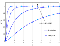
(a) The CDF of the received SNR for different transmit SNR values,$\eta_{t}$, when $N=K=4$, and $\mathbf{u}=\mathbf{a}_{k}$.

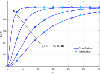
(b) The CDF of the received SNR for different transmit SNR values,$\eta_{t}$, when $N=6,\,K=4$, and $\mathbf{u}=\mathbf{a}_{k}$.

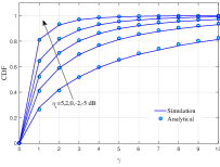
(c) The CDF of the received SNR for different transmit SNR values,$\eta_{t}$, when $N=K=2$, and $\mathbf{u}=\frac{1}{K}\mathbf{1}$.

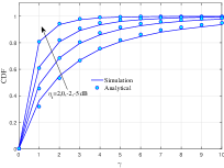
(d) The CDF of the received SNR for different transmit SNR values,$\eta_{t}$, when $N=K=3$, and $\mathbf{u}=\frac{1}{K}\mathbf{1}$.

(e) The CDF of the received SNR for different transmit SNR values,$\eta_{t}$, when $N=8,\,K=5$, and $\mathbf{u}=\frac{1}{K}\mathbf{1}$.

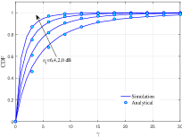
(f) The CDF of the received SNR for different transmit SNR values,$\eta_{t}$, when $N=K=3$, and $u_{k}=0.2$.

Figure 1: The CDF of the received SNR for different values of the transmit SNR, $\eta_{t}$, number of users $K$, number of BS antennas $N$ and $\mathbf{u}$.

Firstly, in Fig. 1 we plot the CDF of the received SNR at the $k^{th}$ user for different values of the transmit SNR, $\eta_{t}$, number of users, $K$, number of BS antennas, $N$, and the vector $\mathbf{u}$. The analytical and simulation results are in well agreement, which confirms the accuracy of the distribution considered in Section (III). In addition, from these results it is clear that, the values of the elements of $\mathbf{u}$ have impact on the CDF and thus on the system performance in general. In this regard it is noted that, user $k$ can achieve the optimal performance when $u_{k}=1$, which is the case presented in Figs. 1a and 1b. Furthermore, the CDF of the received SNR for different values of $N$ and $K$ when the elements of $\mathbf{u}$ have same value, $u_{k}=\frac{1}{K}$, are presented in Figs. 1c, 1d, and 1e and when $u_{k}$ has the smallest value is presented in Fig. 1f. In all these cases the variance of the received SNR will be reduced by the value of $u_{k}$, and thus smaller value of $u_{k}$ will result in poorer/weaker performance/SNR of user $k$ in the system. Finally, it is worthy mentioning that, the results presented in Fig. 1, can be used also to present the outage probability of CI precoding technique. The outage probability is the probability that the received SNR, $\gamma_{k}$, falls below an acceptable threshold value, $\gamma_{th}$. Therefore, we can obtain the outage probability of CI precoding by replacing $\gamma$ with $\gamma_{th}$.

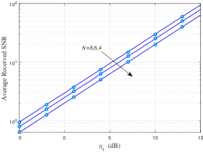
(a) Average received SNR versus transmit SNR,$\eta_{t}$, for different values of $N$ when $K=4$.

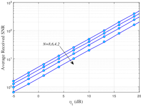
(b) Average received SNR versus transmit SNR,$\eta_{t}$ , for different values of $N$ when $K=2$.

Figure 2: Average received SNR versus transmit SNR, $\eta_{t}$, for different values of $N$ and $K$.

Fig. 2, illustrates the average received SNR versus the transmit SNR, $\eta_{t}$, for different values of $N$ and $K$. Fig. 2a, presents the average received SNR when $K=4$ and Fig. 2b, shows the average received SNR when $K=2$. The good matching between the analytical and simulation results confirms the derived expressions in Section (III-A). Generally and as anticipated, increasing the transmit SNR, number of antennas and/or number of users lead to enhance the average received SNR. In addition, the gain attained by increasing number of the antennas is almost fixed with the transmit SNR in the all considered scenarios.

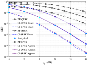
(a) SEP versus transmit SNR, $\eta_{t}$, with different types of input, when $N=K=4$.

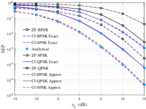
(b) SEP versus transmit SNR, $\eta_{t}$, with different types of input, when $N=6,\,K=4$.

Figure 3: SEP versus transmit SNR for various input types, when $N=4,6\textrm{ and }K=4$.

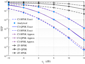
(a) SEP versus transmit SNR, $\eta_{t}$, with different types of input, when $N=K=6$.

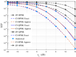
(b) SEP versus transmit SNR, $\eta_{t}$, with different types of input, when $N=8,\,K=6$.

Figure 4: SEP versus transmit SNR for various input types, when $N=6,8\textrm{ and }K=6$.

Fig. 3, shows the exact and approximated average SEP versus transmit SNR, $\eta_{t}$, for different types of input, BPSK, QPSK and 8-PSK. Fig. 3a, presents the average SEP when $N=K=4$, and Fig. 3b, illustrates the average SEP when $N=6,\,\textrm{ and }K=4$. Additionally and for seek of comparison, some results of the conventional interference suppression, ZF, technique are also included in these figures. It should be pointed out that the analytical results in these figures are obtained from the expressions derived in Section (IV). Several interesting points can be extracted from this figure. Firstly, it is evident that the SEP reduces with increasing the transmit SNR, $\eta_{t}$, and CI precoding technique always outperforms the ZF technique in the all SNR values with an up to 15dB gain in the transmit SNR for a given SEP. In addition, it is clear that the approximated results obtained from Section (IV-B) are very tight to the exact ones. Finally, comparing Fig. 3a and Fig. 3b, we can see that, increasing number of BS antennas always enhances the average SEP, and reduces the gap performance between the two precoding techniques.

In order to investigate the impact of number of users and number of BS antennas on the average SEP, in Fig. 4 we present the average SEP for the CI and ZF precoding techniques for BPSK, QPSK and 8PSK, when $N=K=6$, as in Fig. 4a and when $N=8,K=6$ as in Fig. 4b. From the results in Figs. 4 and 3, it is obvious that increasing number of BS antennas $N$ and/or number of users $K$ lead to enhance the system performance. Furthermore, the CI precoding has always better performance than ZF in the all SNR values with an up to 20dB gain in the transmit SNR for a given SEP. In addition, comparing the average SEP in Fig. 4a and Fig. 4b, similar observations can be concluded as in the previous case when $K=4$.

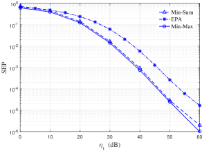
(a) SEP versus transmit SNR, $\eta_{t}$, with different power allocation schemes and QPSK input, when $N=K=3$.

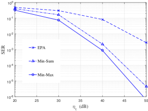
(b) SEP versus transmit SNR, $\eta_{t}$, with different power allocation schemes and QPSK input, when $N=K=8$.

Figure 5: SEP versus transmit SNR with different power allocation schemes.

Fig. 5 illustrates the average SEP versus the transmit SNR, $\eta_{t}$, for different power allocation schemes, EPA, Min-Sum and Min-Max schemes. Fig. 5a, presents the average SEP versus $\eta_{t}$ when $N=K=3$, while Fig. 5b, presents the average SEP versus $\eta_{t}$ when $N=K=8$. From this figure it can be observed that, EPA scheme always results in the highest SEP in the all cases. Therefore, we can say EPA scheme provides the lower bound of the average SEP for the considered MU-MIMO system. In addition, looking closer at the results in Fig. 5a and Fig. 5b one can clearly observe that, the SEP is dominated by the performance of the worst user, and thus the Min-Max scheme has the best performance. It is also noted that, in low transmit SNR values Min-Sum scheme allocates most the transmission power to the best/ closest user to the BS and small amount of power to the farther users, whilst Min-Max scheme allocates relatively high transmission power to the farther user and small amount of power to the near users. In addition, as the transmit SNR value increases Min-Sum scheme starts gradually increasing the power allocated to the farther users at the expense of the power allocated to the near users.

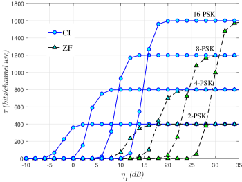
Figure 6: Throughput versus transmit SNR, $\eta_{t}$, for various input types, when $\mathscr{N}=100,$ $Q=5$, and $N=K=4$.

In Fig. 6 we present the throughput versus the transmit SNR, $\eta_{t}$, for different types of input, BPSK, QPSK, 8-PSK and 16-PSK. For seek of comparison, results of the conventional ZF precoding technique are included in the figure. The results in this figure are obtained from the expressions provided in Section (VI). It is evident that the throughput saturates to the value of, $\log_{2}\left(M\right)\times\mathscr{N}\times K$, past a certain transmit SNR $\eta_{t}$ value, the throughput saturates at 400 bits/channel use in BPSK, at 800 bits/channel use in QPSK, at 1200 bits/channel use in 8-PSK and at 1600 bits/channel use in 16-PSK. In addition, the CI precoding outperforms the conventional ZF scheme for a wide range with an up to 15dB gain in the transmit SNR for a given throughput value. Finally and as anticipated, in low SNR values the lower modulation orders have better performance than the higher ones, for instance at 0 dB BPSK achieves the highest throughput. However, in high SNR values the higher modulation orders achieve better performance, for instance at 20 dB 16-PSK has optimal performance.

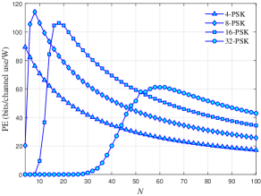
(a) Power Efficiency versus number of BS antennas, $N$, for various input types, when $\mathscr{N}=100,$ $Q=10$, and $K=4$.

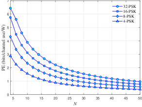
(b) Power Efficiency versus number of BS antennas, $N$, for various input types, when $\mathscr{N}=100,$ $Q=10$, and $K=4$.

Figure 7: Power Efficiency versus number of BS antennas, $N$, for different values of the transmission power.

Finally, Fig. 7 depicts the power efficiency as function of number of BS antennas, $N$, for different values of the transmission power. The results in these figures are obtained from the power efficiency expression provided in Section (IV). In Fig. 7a we present the power efficiency versus $N$ when $\varsigma_{DC}$=0.075, $\varsigma_{MS}=0.09$, $P_{P}=35\textrm{ dbm}$, $\eta_{pa}=0.8$, $P_{D}=7.8\,\textrm{mW}$, $P_{m}=15.2\,\textrm{mW}$, $P_{f}=10\,\textrm{mW}$, $P_{sy}=25\,\textrm{mW}$, and $P_{DS}=2\textrm{W}$ [43, 44, 45]. From Fig. 7a we can observe that when number of BS antennas is small the lower modulation orders achieve higher power efficiency than the higher orders, for instance when $N=4$ QPSK has best performance. On the other hand, when number of BS antennas is large the higher modulation orders become better than the lower ones, for instance 32-PSK achieves the highest power efficiency when $N=60$. Furthermore, in order to clearly demonstrate the impact of transmission power on the power efficiency for different types of input, we plot in Fig. 7b the power efficiency versus $N$ when the transmission power is very high $P_{P}=20\textrm{ dbW}$. In this case, the higher modulation orders always have better system performance regardless number of antennas implemented at the BS. Furthermore, comparing Figs. 7a and 7b it can be concluded that, the power efficiency achieved in low transmit SNR is much higher than that in high transmit SNR regime.

VIII Conclusions

In this paper the statistics of the received SNR of CI precoding technique has been considered for the first time. Firstly, exact closed form expressions of the MGF and the average received SNR have been derived. Then, the derived MGF expression was used to calculate the average SEP. In light of this, exact average SEP expression for CI precoding with $M$-PSK was obtained. In addition, accurate asymptotic approximation for the average SEP has been provided. Building on the new performance analysis, different power allocation schemes to enhance the average SEP have been considered. In the first scheme, power allocation technique based on minimizing the total SEP was studied, while in the second scheme power allocation technique based on minimizing the maximum SEP was investigated. Furthermore, new and explicit analytical expressions of the throughput and power efficiency of the CI precoding in MU-MIMO systems have been derived. The results in this paper explained that the CI scheme outperforms ZF scheme in the all considered metrics. Furthermore, increasing the transmit SNR, number of users and number of BS antennas always enhance the achieved SEP. It was also shown that, using EPA leads to the highest SEP and the considered power allocation techniques can perform very low SEP. Finally, in low transmit SNR values and when number of BS antennas is small, the lower modulation orders achieve higher power efficiency than the higher modulation orders.

References

• [1] A. Salem and C. Masouros, “On the error probability of interference exploitation precoding with power allocation,” in Proc. IEEE Wireless Commun. Netw. Conf. (WCNC), 2020.
• [2] M. S. John G. Proakis, Digital Communications, Fifth Edition.   McGraw-Hill, NY USA, 2008.
• [3] C. B. P. Howard Huang and S. Venkatesan, MIMO Communication for cellular Networks.   Springer, 2012, 2008.
• [4] Y. Wu, C. Xiao, X. Gao, J. D. Matyjas, and Z. Ding, “Linear precoder design for mimo interference channels with finite-alphabet signaling,” IEEE Transactions on Communications, vol. 61, no. 9, pp. 3766–3780, September 2013.
• [5] A. Salem and K. A. Hamdi, “Wireless power transfer in multi-pair two-way af relaying networks,” IEEE Transactions on Communications, vol. 64, no. 11, pp. 4578–4591, Nov 2016.
• [6] W. Wu, K. Wang, W. Zeng, Z. Ding, and C. Xiao, “Cooperative multi-cell mimo downlink precoding with finite-alphabet inputs,” IEEE Transactions on Communications, vol. 63, no. 3, pp. 766–779, March 2015.
• [7] M. Costa, “Writing on dirty paper (corresp.),” IEEE Transactions on Information Theory, vol. 29, no. 3, pp. 439–441, May 1983.
• [8] C. Masouros, M. Sellathurai, and T. Ratnarajah, “Maximizing energy efficiency in the vector precoded mu-miso downlink by selective perturbation,” IEEE Transactions on Wireless Communications, vol. 13, no. 9, pp. 4974–4984, Sep. 2014.
• [9] A. Garcia-Rodriguez and C. Masouros, “Power-efficient tomlinson-harashima precoding for the downlink of multi-user miso systems,” IEEE Transactions on Communications, vol. 62, no. 6, pp. 1884–1896, June 2014.
• [10] A. Li and C. Masouros, “Interference exploitation precoding made practical: Optimal closed-form solutions for psk modulations,” IEEE Transactions on Wireless Communications, pp. 1–1, 2018.
• [11] T. Haustein, C. von Helmolt, E. Jorswieck, V. Jungnickel, and V. Pohl, “Performance of mimo systems with channel inversion,” in Vehicular Technology Conference. IEEE 55th Vehicular Technology Conference. VTC Spring 2002 (Cat. No.02CH37367), vol. 1, May 2002, pp. 35–39 vol.1.
• [12] C. B. Peel, B. M. Hochwald, and A. L. Swindlehurst, “A vector-perturbation technique for near-capacity multiantenna multiuser communication-part i: channel inversion and regularization,” IEEE Transactions on Communications, vol. 53, no. 1, pp. 195–202, Jan 2005.
• [13] A. Wiesel, Y. C. Eldar, and S. Shamai, “Linear precoding via conic optimization for fixed mimo receivers,” IEEE Transactions on Signal Processing, vol. 54, no. 1, pp. 161–176, Jan 2006.
• [14] M. F. Hanif, L. Tran, A. Tölli, and M. Juntti, “Computationally efficient robust beamforming for sinr balancing in multicell downlink with applications to large antenna array systems,” IEEE Transactions on Communications, vol. 62, no. 6, pp. 1908–1920, June 2014.
• [15] M. Schubert and H. Boche, “Solution of the multiuser downlink beamforming problem with individual sinr constraints,” IEEE Transactions on Vehicular Technology, vol. 53, no. 1, pp. 18–28, Jan 2004.
• [16] N. D. Sidiropoulos, T. N. Davidson, and Zhi-Quan Luo, “Transmit beamforming for physical-layer multicasting,” IEEE Transactions on Signal Processing, vol. 54, no. 6, pp. 2239–2251, June 2006.
• [17] C. Masouros and E. Alsusa, “Dynamic linear precoding for the exploitation of known interference in mimo broadcast systems,” IEEE Transactions on Wireless Communications, vol. 8, no. 3, pp. 1396–1404, March 2009.
• [18] C. Masouros, M. Sellathurai, and T. Ratnarajah, “Vector perturbation based on symbol scaling for limited feedback miso downlinks,” IEEE Transactions on Signal Processing, vol. 62, no. 3, pp. 562–571, Feb 2014.
• [19] C. Masouros and G. Zheng, “Exploiting known interference as green signal power for downlink beamforming optimization,” IEEE Transactions on Signal Processing, vol. 63, no. 14, pp. 3628–3640, July 2015.
• [20] P. V. Amadori and C. Masouros, “Large scale antenna selection and precoding for interference exploitation,” IEEE Transactions on Communications, vol. 65, no. 10, pp. 4529–4542, Oct 2017.
• [21] S. Timotheou, G. Zheng, C. Masouros, and I. Krikidis, “Exploiting constructive interference for simultaneous wireless information and power transfer in multiuser downlink systems,” IEEE Journal on Selected Areas in Communications, vol. 34, no. 5, pp. 1772–1784, May 2016.
• [22] M. R. A. Khandaker, C. Masouros, and K. K. Wong, “Constructive interference based secure precoding: A new dimension in physical layer security,” IEEE Transactions on Information Forensics and Security, vol. 13, no. 9, pp. 2256–2268, Sept 2018.
• [23] A. Haqiqatnejad, F. Kayhan, and B. Ottersten, “Symbol-level precoding design based on distance preserving constructive interference regions,” IEEE Transactions on Signal Processing, vol. 66, no. 22, pp. 5817–5832, Nov 2018.
• [24] ——, “Constructive interference for generic constellations,” IEEE Signal Processing Letters, vol. 25, no. 4, pp. 586–590, April 2018.
• [25] A. Salem, C. Masouros, and K. Wong, “Sum rate and fairness analysis for the mu-mimo downlink under psk signalling: Interference suppression vs exploitation,” IEEE Transactions on Communications, pp. 1–1, 2019.
• [26] A. Salem, C. Masouros, and B. Clerckx, “Rate Splitting with Finite Constellations: The Benefits of Interference Exploitation vs Suppression,” arXiv e-prints, p. arXiv:1907.08457, Jul 2019.
• [27] R. J. Muirhead, Aspects of Multivariate Statistical Theory, 1982.
• [28] M. L. Eaton, Chapter 8: The Wishart Distribution, ser. Lecture Notes–Monograph Series.   Beachwood, Ohio, USA: Institute of Mathematical Statistics, 2007, vol. Volume 53, pp. 302–333. [Online]. Available: https://doi.org/10.1214/lnms/1196285114
• [29] M. Abramowitz and I. A. Stegun, Handbook of Mathematical Functions With Formulas, Graphs, and Mathematical Tabl, Washington,D.C.: U.S. Dept. Commerce, 1972.
• [30] M. K. Simon and M. S. Alouini, Digital Communication over Fading Channels.   John wiley and Sons, Inc., 2000.
• [31] M. R. Mckay, A. Zanella, I. B. Collings, and M. Chiani, “Error probability and sinr analysis of optimum combining in rician fading,” IEEE Transactions on Communications, vol. 57, no. 3, pp. 676–687, March 2009.
• [32] M. Chiani, D. Dardari, and M. K. Simon, “New exponential bounds and approximations for the computation of error probability in fading channels,” IEEE Transactions on Wireless Communications, vol. 2, no. 4, pp. 840–845, July 2003.
• [33] S. Boyd and L. Vandenberghe, Convex Optimization.   Cambridge, UK: Cambridge University. Press, 2004.
• [34] H. David., Order Statistics, 1970:John Wiley and Sons.
• [35] C. Masouros, “Correlation rotation linear precoding for mimo broadcast communications,” IEEE Transactions on Signal Processing, vol. 59, no. 1, pp. 252–262, Jan 2011.
• [36] A. T. Toyserkani, E. G. Strom, and A. Svensson, “An analytical approximation to the block error rate in nakagami-m non-selective block fading channels,” IEEE Transactions on Wireless Communications, vol. 9, no. 5, pp. 1543–1546, May 2010.
• [37] R. Eaves and A. Levesque, “Probability of block error for very slow rayleigh fading in gaussian noise,” IEEE Transactions on Communications, vol. 25, no. 3, pp. 368–374, March 1977.
• [38] F. Adachi and T. Matsumoto, “Double symbol error rate and block error rate of mdpsk,” Electronics Letters, vol. 27, no. 17, pp. 1571–1573, Aug 1991.
• [39] A. Seyoum and N. C. Beaulieu, “Semianalytical simulation for evaluation of block-error rates on fading channels,” IEEE Transactions on Communications, vol. 46, no. 7, pp. 916–920, July 1998.
• [40] M. Ruiz-Garcia, J. M. Romero-Jerez, C. Tellez-Labao, and A. Diaz-Estrella, “Average block error probability of multicell cdma packet networks with fast power control under multipath fading,” IEEE Communications Letters, vol. 6, no. 12, pp. 538–540, Dec 2002.
• [41] Jianhua Lu, K. B. Letaief, J. C. . Chuang, and M. L. Liou, “M-psk and m-qam ber computation using signal-space concepts,” IEEE Transactions on Communications, vol. 47, no. 2, pp. 181–184, Feb 1999.
• [42] M. Chiani, “Error probability for block codes over channels with block interference,” IEEE Transactions on Information Theory, vol. 44, no. 7, pp. 2998–3008, Nov 1998.
• [43] A. Garcia-Rodriguez and C. Masouros, “Exploiting the increasing correlation of space constrained massive mimo for csi relaxation,” IEEE Transactions on Communications, vol. 64, no. 4, pp. 1572–1587, April 2016.
• [44] G. Auer, V. Giannini, I. Godor, P. Skillermark, M. Olsson, M. A. Imran, D. Sabella, M. J. Gonzalez, C. Desset, and O. Blume, “Cellular energy efficiency evaluation framework,” in 2011 IEEE 73rd Vehicular Technology Conference (VTC Spring), May 2011, pp. 1–6.
• [45] H. Kim, C. Chae, G. de Veciana, and R. W. Heath, “A cross-layer approach to energy efficiency for adaptive mimo systems exploiting spare capacity,” IEEE Transactions on Wireless Communications, vol. 8, no. 8, pp. 4264–4275, August 2009.