Density-functional model for van der Waals interactions:
Unifying many-body atomic approaches with nonlocal functionals

Van der Waals (vdW) interactions originate from nonlocal correlations in the quantum motion of electrons and give rise to a wide spectrum of physical phenomena from attraction between two atoms (London, 1930) to the macroscopic Casimir effect (Jaffe, 2005). As a result, vdW interactions are one of the prime targets in material modeling, which has led to a plethora of approaches that either treat vdW forces in the same way as the rest of electron correlation, or model them with effective potentials (Klimeš and Michaelides, 2012; Grimme et al., 2016; Hermann et al., 2017). They include quantum Monte–Carlo (QMC) (Ambrosetti et al., 2014a), coupled cluster methods (Yang et al., 2014), random-phase approximation (Lu et al., 2009), nonlocal density functionals (Dion et al., 2004; Vydrov and Van Voorhis, 2009), and coarse-grained approaches ranging from pairwise (Grimme et al., 2010; Becke and Johnson, 2007; Tkatchenko and Scheffler, 2009) to many-body models (Tkatchenko et al., 2012; Silvestrelli, 2013; Caldeweyher et al., 2019).

From a theoretical perspective, this status quo is undesirable, because different models offer often disparate pictures of the nature of vdW forces, leading to incoherent understanding of vdW interactions in molecules and materials. From a practical perspective, the three main characteristics of a method are its generality, accuracy, and computational efficiency, and so far, no single method has satisfied all three requirements while being applicable to all relevant types of matter. For instance, QMC and coupled cluster are limited by computational efficiency, pairwise approaches and two-point vdW functionals lack in accuracy for nanostructured and supramolecular compounds, and atomic models have qualitative problems with ionic and hybrid metal-organic systems.

In this work, we present a unified density-functional model of vdW interactions that couples polarizability density functionals and atomic models, inheriting broad applicability of the former and excellent accuracy of the latter. We integrate the polarizability functional of Vydrov and Van Voorhis (2010b) (VV), normalization to exact free-atom vdW parameters of the Tkatchenko–Scheffler (TS) model (Tkatchenko and Scheffler, 2009), normalization to jellium via a zero-gradient limit from the VV10 functional (Vydrov and Van Voorhis, 2010a), and the Hamiltonian for the dispersion energy of the many-body dispersion (MBD) model (Tkatchenko et al., 2013). Compared to the range-separated self-consistently screened (rsSCS) variant of MBD (Ambrosetti et al., 2014b), the VV polarizability functional enables consistent treatment of ionic compounds, normalization to the free-atom reference balances the accuracy of the VV polarizability across the periodic table, and normalization to jellium enables effective modeling of metals and their surfaces (Ruiz et al., 2012). The new model involves a similar level of empiricism as MBD@rsSCS—we remove the tabulated vdW radii and short-range screening, while introducing a mechanism to avoid double counting of electron correlation in near-uniform density regions. We demonstrate on a series of benchmark calculations that the new model enables for the first time a consistent treatment of vdW interactions in molecular, covalent, ionic, metallic, and hybrid metal-organic systems.

Some of the problems of MBD@rsSCS have been previously treated by Gould et al. (2016). Their fractionally ionic variant of MBD@rsSCS uses iterative Hirshfeld partitioning in combination with a piecewise linear dependence of atomic polarizability on charge, together with a rescaling scheme for the diverging MBD Hamiltonian in highly polarizable systems or with dipole smearing (Kim et al., 2020). Our approach is instead based on a general polarizability functional.

Atomic models, such as MBD, require an atomic response model in the form of static polarizabilities $\alpha_{0,i}\equiv\alpha_{i}(0)$ and $C_{6,ii}$ coefficients. In the new model, dubbed MBD-NL, we parametrize the response of atoms by coarse-graining the VV polarizability density to atomic fragments (Hirshfeld, 1977; Sato and Nakai, 2009, 2010). The VV polarizability functional is a semilocal functional of the electron density $n(\mathbf{r})$, which models the local dynamic polarizability density (Vydrov and Van Voorhis, 2010b),

$$\alpha^{\text{VV}}[n](\mathbf{r},\mathrm{i}u)=\frac{n(\mathbf{r})}{\frac{4\pi}{3}n(\mathbf{r})+C\frac{{|\boldsymbol{\nabla}n(\mathbf{r})|}^{4}}{n{(\mathbf{r})}^{4}}+u^{2}}$$ (1)

where $\mathrm{i}u$ is imaginary frequency and $C$ is an empirical parameter. The atomic dynamic polarizabilities are obtained by partitioning the polarizability density with Hirshfeld weights $w_{i}^{\text{H}}(\mathbf{r})=n_{i}^{\text{free}}(\mathbf{r})/\sum_{j}n_{j}^{\text{free}}(\mathbf{r})$,

$$\alpha_{i}^{\text{VV}}(\mathrm{i}u)=\int\mathrm{d}\mathbf{r}\,w_{i}^{\text{H}}(\mathbf{r})\alpha^{\text{VV}}[n](\mathbf{r},\mathrm{i}u)$$ (2)

The $C_{6}$ coefficients are then calculated directly from $\alpha_{i}(\mathrm{i}u)$ via the Casimir–Polder formula (McLachlan, 1963),

$$C_{6,ii}^{\text{VV}}=\frac{3}{\pi}\int_{0}^{\infty}\mathrm{d}u\,\alpha_{i}^{\text{VV}}{(\mathrm{i}u)}^{2}$$ (3)

Unlike approaches that use Hirshfeld fragments to define atomic volumes, MBD-NL is independent of the choice of a particular atomic partitioning, because this influences only local redistribution of the polarizability between atoms, conserving the total polarizability. Our approach is also different from that of Silvestrelli (2008), where the electron density is coarse-grained first and a polarizability functional is evaluated over the fragment densities.

Already this bare combination of MBD and the VV polarizability functional substantially improves the description of ionic systems compared to MBD@rsSCS, because the VV functional gives a good estimate of the ionic polarizabilities, unlike the Hirshfeld volume scaling used in MBD@rsSCS. However, this bare combination suffers from two fundamental shortcomings. First, the polarizability functional is not evenly accurate across the periodic table. Second, when combined with semilocal density-functional theory (DFT), it suffers from double counting of electron correlation in regions of slowly-varying electron density. To solve these two challenges, we normalize the atomic VV polarizabilities and $C_{6}$ coefficients to exact values for free atoms (Tkatchenko and Scheffler, 2009), and then normalize MBD-NL to give zero vdW energy for jellium by subtracting the portion of the polarizability from slowly-varying electron-density regions.

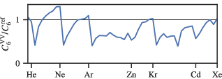
Figure 1: Relative errors in $C_{6}$ coefficients of free atoms calculated with the VV polarizability functional for the first 54 elements. The reference values are taken from the TS method (Tkatchenko and Scheffler, 2009). In contrast, the present model is exact by construction (Eq. 4).

The VV polarizability functional is approximate, which is manifest already for free-atom polarizabilities and $C_{6}$ coefficients, where accurate reference values are known (Figure 1). It especially underestimates the vdW parameters of metallic elements. To mitigate this, we normalize the VV atomic quantities with the ratio of the respective free-atom values obtained from accurate reference calculations and from the VV functional,

$$\alpha_{0,i}^{\text{rVV}}=\alpha_{0,i}^{\mathrm{VV}}\frac{\alpha_{0,i}^{\text{ref,free}}}{\alpha_{0,i}^{\text{VV,free}}},\quad C_{6,ii}^{\text{rVV}}=C_{6,ii}^{\mathrm{VV}}\frac{C_{6,ii}^{\text{ref,free}}}{C_{6,ii}^{\text{VV,free}}}$$ (4)

Many exchange–correlation (XC) functionals are exact for jellium by construction, even though the portion of electron correlation from the nonlocal plasmons is long-ranged and should not be included in semilocal XC functionals. As a result, most XC functionals describe accurately the electron correlation within slowly-varying density regions, such as found in metals, and those cases require no addition of vdW forces. This is different in most general systems, in which semilocal functionals neglect long-range vdW interactions. At the same time, these metallic-density regions contribute dominantly to the VV polarizability, and hence to the vdW energy in any vdW model that would use the VV functional directly. When combined with semilocal DFT, this would result in overpolarization and overbinding of bulk metals, and of adsorbates on metallic surfaces. To avoid this double counting, the VV10 expression for the vdW energy subtracts the limit of VV10 as the density gradient approaches zero (Vydrov and Van Voorhis, 2010a), $E_{\text{vdW}}^{\text{VV10}}=E^{\text{VV10}}[n]-\bigl{(}E^{\text{VV10}}|_{\boldsymbol{\nabla}n\rightarrow 0}\bigr{)}[n]$. Such an approach cannot be used directly in a many-body model such as MBD, because unlike in a pairwise model the many-body vdW energy is not linear in the polarizability.

To ensure the correct zero limit of MBD-NL for uniform densities, we smoothly cut off the contribution of jellium-like regions to the polarizability. These regions can be distinguished with the combination of two local electron-density descriptors: the local ionization potential $I$ (Gutle et al., 1999) and the iso-orbital indicator $\chi$ (Becke and Edgecombe, 1990; Kümmel and Perdew, 2003; Sun et al., 2013),

$$I[n]=\frac{\tau^{\text{W}}[n]}{n},\qquad\chi[n]=\frac{\tau^{\text{KS}}[n]-\tau^{\text{W}}[n]}{\tau^{\text{unif}}[n]}$$ (5)

where $\tau^{\text{KS}}[n]=\sum_{i}|\boldsymbol{\nabla}\phi_{i}|^{2}/2$ is the positive kinetic energy density of occupied orbitals $\phi_{i}$, which for single-orbital densities reduces to the von Weizsäcker kinetic energy density, $\tau^{\text{W}}[n]=|\boldsymbol{\nabla}n|^{2}/8n$, and for jellium to $\tau^{\mathrm{unif}}[n]=3(3\pi^{2})^{2/3}n^{5/3}/10$. The local ionization potential is a form of a reduced gradient with the units of energy, which attempts to model the electronic gap locally. The density gradient alone is insufficient to characterize metallic densities. In particular, both $I\sim 0$ and $\chi\sim 1$ must be true for density to be metallic, whereas $I\sim 0$ and $\chi\sim 0$ corresponds to centers of covalent bonds, and $I\sim 0$ and $\chi\gg 1$ signifies overlap of electron-density tails between noncovalently bound systems. Since the normalization of VV10 to jellium uses only the density gradient, it partially omits contributions from covalent bonds. By using also the iso-orbital indicator, we make MBD-NL more precise in this regard. In practical calculations, the evaluation of the kinetic energy density is the computationally most demanding part of MBD-NL, but this means that its cost is only a fraction of a single self-consistent cycle of a regular meta-GGA KS-DFT calculation.

Figure 2: Polarizability distributions of local ionization potential $I$ and iso-orbital indicator $\chi$. The plotted distributions are $\alpha^{\text{VV}}(s^{\prime},\chi^{\prime})=\int\mathrm{d}\mathbf{r}\delta(s(\mathbf{r})-s^{\prime})\delta(\chi(\mathbf{r})-\chi^{\prime})\alpha^{\text{VV}}(\mathbf{r})$, such that the total polarizability is $\iint\mathrm{d}s\mathrm{d}\chi\,\alpha^{\text{VV}}(s,\chi)$. $E_{\text{h}}$ is one hartree. (a) Benzene monomer, dimer, and crystal. Each distribution is normalized to one benzene molecule. (b) 64 simple solids divided to five groups (Zhang et al., 2018). Each distribution is normalized to 62 (a. u.), the VV polarizability of a benzene monomer, for a single color scale with a.

Figure 2a presents polarizability density distributions of $I$ and $\chi$ in three benzene compounds and in a set of simple solids (Zhang et al., 2018). In an organic molecule such as benzene (Figure 2a), the vast majority of the polarizability comes from electron density with $I>$5\text{\,}\mathrm{eV}$$, with a small part from low-gradient regions with $\chi<1$. The intermolecular interactions in the benzene dimer and crystal add a significant amount of polarizability in regions with $\chi\gg 1$, despite the electron density being low there. A richer spectrum of patterns is found in simple solids (Figure 2b). Most similar to the benzene compounds are semiconductors. In contrast, the polarizability in main-group metals is dominated by jellium-like regions near $(I,\chi)=(0,1)$. In transition metals, the polarizability is distributed in a wider range of the local gap along the $1<\chi<2$ strip, with a larger part still in the low-gradient regions. In simple ionic solids, most of the polarizability comes from single-orbital regions ($\chi<1$).

To avoid the double counting of vdW interactions of low-gradient densities, we smoothly cut off their contribution to the polarizability functional,

$$\alpha^{\mathrm{VV^{\prime}}}[n](\mathbf{r})=g(I,\chi)\alpha^{\text{VV}}[n]$$ (6)

We impose two simple requirements on this cutoff. First, the density regions with a local gap lower than the work function of conductors should not contribute to the calculated vdW energy, because those are assumed to be covered by a semilocal XC functional. We chose the cutoff value of 5 eV, which is around the peak of the work function of elemental metals. Second, the VV polarizability of simple covalent compounds (exemplified by a benzene molecule) should not be influenced by the cutoff. The following function $g$ satisfies these two requirements:

$$\begin{gathered}g(I,\chi)=1-\frac{1-f\bigl{(}\chi-3\sqrt{I/E_{\text{h}}}\bigr{)}}{1+\exp\bigl{(}4(I-$5\text{\,}\mathrm{eV}$)/$1\text{\,}\mathrm{eV}$\bigr{)}},\\ f(x)=\exp\bigl{(}-\theta(x)cx/(1-x)\bigr{)}\theta(1-x)\end{gathered}$$ (7)

Function $g$ consists of a logistic function centered at $5\text{\,}\mathrm{eV}$ and of function $f$ taken from the SCAN functional (Sun et al., 2015), where it also interpolates between $\chi=0$ and $\chi=1$ (see Appendix for a plot of $g(I,\chi)$). We find that $c=1/10$ ensures that the effect of the cutoff on the VV polarizability of a benzene molecule is negligible ($<2\%$). The performance of the resulting model depends only weakly on the precise values of the chosen parameters, as long as the local gap cutoff sufficiently covers the work function of a given conductor. Nevertheless, a more rigorous formulation of the model in this direction would be desirable.

Figure 3: Distributions of relative changes in atomic static polarizabilities and $C_{6}$ coefficients from monomers to dimers. The distributions are calculated over all atoms from all complexes in the S66 data set (Řezáč et al., 2011).

Apart from avoiding the double counting of long-range electron correlation, the cutoff function removes another deficiency of the VV polarizability functional. When molecules form vdW-bound compounds, the introduction of density-tail overlaps significantly increases the VV polarizability compared to the monomers (Figure 2a). This effect is an artifact of the VV functional that causes increasingly large vdW-bound systems to be overbound, and cutting off the polarizability of low-gradient regions with $\chi>1$ eliminates this issue without affecting the polarizabilities of isolated monomers (Figure 3).

Finally, the static polarizabilities and $C_{6}$ coefficients calculated as described above are directly used in the MBD Hamiltonian to obtain the vdW energy. This Hamiltonian describes a system of charges in harmonic potentials—Drude oscillators—characterized by their static polarizabilities $\alpha_{0,i}$ and resonance frequencies $\omega_{i}=4C_{6,ii}/3\alpha_{0,i}^{2}$, and interacting via a long-range dipole potential $\mathbf{T}^{\mathrm{lr}}(\mathbf{R})\equiv f_{\text{lr}}(R)\mathbf{T}(\mathbf{R})$ (Lucas, 1967; Tkatchenko et al., 2012),

$$H^{\text{MBD}}(\{\alpha_{0,i},\omega_{i}\})=\sum_{i}-\frac{1}{2}\nabla_{\xi_{i}}^{2}+\sum_{i}\frac{1}{2}\omega_{i}^{2}\xi_{i}^{2}\\ +\frac{1}{2}\sum_{ij}\omega_{i}\omega_{j}\sqrt{\alpha_{0,i}\alpha_{0,j}}\boldsymbol{\xi}_{i}\cdot\mathbf{T}^{\mathrm{lr}}_{ij}\boldsymbol{\xi}_{j}$$ (8)

where $\boldsymbol{\xi}_{i}\equiv\sqrt{m_{i}}\mathbf{x}_{i}$ are displacements of the charges weighted with masses $m_{i}$ (which have no effect on the energy). The interaction energy of this model system—the vdW energy—is obtained by direct diagonalization yielding a set of coupled oscillation frequencies $\tilde{\omega}_{k}$,

$$E_{\text{MBD}}=\sum_{k}^{3N}\frac{\tilde{\omega}_{k}}{2}-\sum_{i}^{N}\frac{3\omega_{i}}{2}$$ (9)

In MBD-NL, we use the same long-range coupling $\mathbf{T}^{\text{lr}}$ as in the MBD@rsSCS variant (Ambrosetti et al., 2014b),

$$f_{\text{lr}}(R_{ij})=1\Big{/}\Big{(}1+\mathrm{e}^{-6{\textstyle(}R_{ij}/\beta(R_{i}^{\text{vdW}}+R_{j}^{\text{vdW}})-1{\textstyle)}}\Big{)}$$ (10)

but with a simplified definition of the vdW radii. Rather than tabulated vdW radii, we use the quantum-mechanical formula for vdW radii of free atoms from Fedorov et al. (2018), and scale them similarly to the vdW parameters as in (4),

$$R_{i}^{\text{vdW}}=\tfrac{5}{2}{(\alpha_{0,i}^{\text{ref,free}})}^{\frac{1}{7}}{\left(\frac{\alpha_{i}^{\mathrm{rVV^{\prime}}}}{\alpha_{i}^{\text{rVV${}^{\prime}$,free}}}\right)}^{\frac{1}{3}}$$ (11)

We optimize the damping parameter $\beta$ of $f_{\text{lr}}(R)$ on the S66 data set (Řezáč et al., 2011), as was done for MBD@rsSCS, and find the optimal values of 0.81 and 0.83 for the XC functionals PBE (Perdew et al., 1996) and PBE0 (Adamo and Barone, 1999), respectively, only slightly smaller than the values of 0.83 and 0.85 for MBD@rsSCS.

Figure 4: Distributions of relative errors in binding and lattice energies. The boxes show quartiles of the distributions, the whiskers extend further up to 1.5-fold the inter-quartile range, and the individual points denote outliers. (a) S66$\times$8 set of organic dimers. The color scale encodes the distance between the centers of mass of the monomers, divided by the equilibrium distance. (b) Set of 64 hard solids (Zhang et al., 2018). The color encodes the class of a solid: transition metals (TM), main-group metals (MM), semiconductors (SC), transition-metal carbides and nitrides (TMCN), and ionic crystals (IC). The left-right order of the systems in the plot corresponds to the top-bottom order in the legend.

Next, we briefly describe several benchmark tests of MBD-NL (see Appendix for a more detailed description of the calculations and for additional results). On a set of small organic dimers (S66, Řezáč et al., 2011), MBD-NL performs nearly identically to MBD@rsSCS (Figure 4a), which is already excellent for a DFT+vdW approach. In contrast, the errors in lattice energies of 64 hard solids (Zhang et al., 2018) are reduced drastically when MBD@rsSCS is replaced with MBD-NL (Figure 4b). This improvement comes mainly from the errors for metals and ionic solids, which MBD@rsSCS overbinds substantially, whereas plain PBE performs reasonably well, and MBD-NL retains this good performance. MBD-NL still somewhat overbinds the metals compared to PBE, as could be expected, because bare PBE does not underbind the metals despite the missing (non-jellium) long-range vdW interactions. Ionic solids are underbound by 4% with PBE, which is reduced nearly to zero when the missing nonlocal correlation is added by MBD-NL, whereas MBD@rsSCS overbinds some of them substantially. The performance of MBD-NL on semiconductors is similar to MBD@rsSCS. On a set of organic molecular crystals (X23, Reilly and Tkatchenko, 2013), MBD-NL performs nearly identically to MBD@rsSCS, with a similar tendency to underbind (2%) as MBD@rsSCS has to overbind (3%). On a set of supramolecular complexes (S12L, Grimme, 2012), the accuracy of MBD-NL is reduced compared to MBD@rsSCS, from 5% to 9% in terms of the mean absolute relative error (MARE), but the accuracy of the two methods is equal with the PBE0 functional, with MBD-NL having a smaller mean relative error compared to MBD@rsSCS.

Compounds with small or zero electronic gap pose the hardest problem for DFT+vdW approaches, because such systems require in principle long-range coupling of delocalized electronic fluctuations. Despite that, MBD-NL reaches the accuracy of established effective models for hybrid interfaces of metallic surfaces and organic molecules, such as the MBD@rsSCS[surf] method (Ruiz et al., 2016), with a difference in the binding energy between the two methods below 10% for a benzene molecule on a silver (111) surface. This is only possible because the long-wavelength electronic fluctuations in the metal have no correlation counterpart in the adsorbed molecule, so a fully delocalized treatment of the fluctuations is not necessary in this case.

In contrast, the delocalized fluctuations cannot be effectively neglected in layered vdW materials with small band gaps, such as the transition-metal dichalcogenides (TMDCs), which comprise 23 of the benchmark set of 26 layered materials (here dubbed “26”, Björkman, 2012). MBD@rsSCS and VV10 overbind the “26” set by 10% and 52%, respectively, indicating that both models overpolarize these small-gap layered compounds. In contrast, the nonlocal part of the polarizability from low-gradient density regions is removed in MBD-NL, resulting in its underbinding of the “26” set by 21% (the accuracy of the reference calculations is 10%–20%). Of the three methods, the three non-TMDC layered materials in the “26” set (graphite, BN, PbO) are described most accurately by MBD-NL (MARE of 7%, compared to 27% for MBD@rsSCS and 53% for VV10).

Before concluding, we discuss some open questions regarding MBD-NL. First, the VV polarizability functional is semi-empirical and it can be improved by including nonlocal density information, for example by developing a meta-GGA polarizability functional. Such an extension could improve the overall accuracy significantly, but requires nontrivial advances in the general theory of polarizability functionals. Another possibility would be to normalize the vdW parameters not only to free atoms, but also to ions (Gould et al., 2016), which is comparably more straightforward. Second, although MBD-NL can effectively treat hybrid interfaces between organic and metallic compounds, it does not capture the truly nonlocal electronic fluctuations that can be found in conductors (Dobson, 2014). Incorporating such a mechanism would not only enable MBD-NL to treat long-range interactions between fully metallic bodies, but also increase its accuracy for interacting systems of small-gap compounds, such as TMDCs. How to do this in practice is at the moment unclear, and we see this as the largest remaining theoretical gap in the general understanding of vdW interactions in materials. Third, MBD-NL uses an empirical range-separating function parameterized for a given XC functional. XC functionals differ substantially in their mid-range behavior (unlike the PBE and PBE0 functionals used here), and developing seamless range-separation approaches that couple semilocal XC functionals and vdW methods in a universal and transferable way remains an open challenge (Hermann and Tkatchenko, 2018).

In conclusion, we have developed a vdW model that unifies atomic many-body methods and nonlocal vdW functionals. By normalizing to free atoms and jellium, we have retained the accuracy of best DFT+vdW approaches while extending applicability to ionic and metallic compounds, and hybrid metal-organic interfaces. Our approach enables efficient, accurate, and consistent modeling of many-body vdW interactions in a substantially broader range of systems than previously possible.

Appendix

All computational resources for the manuscript can be found in a Git repository (Hermann, 2019a) and related data files (Hermann, 2019b). This includes scripts used to generate input files, to run the calculations, process and analyze data, and generate figures. The file organization is described in the README.md file in the repository.

All DFT calculations were done with FHI-aims (Blum et al., 2009), which uses atom-centered basis sets with numerical radial parts. We used the tight default basis set and grid settings, which ensure numerical convergence to 0.1 kcal/mol in binding energies for the van der Waals (vdW) systems studied here. MBD calculations were performed with the help of the Libmbd library (Hermann, 2019c), which is integrated into FHI-aims, and MBD-NL calculations can be performed directly in FHI-aims with a current development version. Our current implementation does not include the functional derivative $\delta\alpha^{\text{VV'}}[n]/\delta n$, and as such MBD-NL is evaluated on the self-consistent PBE densities in this work, while the implementation of the derivative is a work in progress. Importantly, the electron density change induced by vdW interactions has been found to have only a negligible effect on the interaction energies and nuclear forces (Ferri et al., 2015). The PBE, PBE0, and VV10 energies for the S66, X23, and S12L sets were taken from (Hermann and Tkatchenko, 2018), which used the same numerical settings as this work. For molecular crystals, $k$-point grids with density of at least 0.8 Å in reciprocal space were used for all DFT and MBD calculations. For hard solids, we have used the $k$-point density from (Zhang et al., 2018). All molecular and crystal geometries were taken directly from the respective benchmark sets without any relaxation.

Table 1: Errors in interaction energies on vdW benchmark data sets.

Method		S66	X23	S12L	“26”a
PBE	MREb	$57$%	$60$%	$82$%	$105$%
+MBD@rsSCS	MAREc	$8.4$%	$6.4$%	$5.3$%	$14$%d
	MRE	$-3.1$%	$-3.4$%	$-1.4$%	$-10$%d
+MBD-NL	MARE	$9.3$%	$6.2$%	$9.2$%	$21$%
	MRE	$-0.1$%	$1.9$%	$6.4$%	$21$%
+VV10	MARE	$9.9$%	$15$%	$15$%	$52$%e
	MRE	$-6.1$%	$-15$%	$-15$%	$-52$%e
PBE0	MRE	$56$%	$58$%	$75$%
+MBD@rsSCS	MARE	$7.6$%	$5.4$%	$6.5$%
	MRE	$-1.1$%	$-1.7$%	$-4.4$%
+MBD-NL	MARE	$8.5$%	$5.7$%	$6.8$%
	MRE	$0.0$%	$3.0$%	$1.7$%
+VV10	MARE	$8.3$%	$15$%	$20$%
	MRE	$-5.3$%	$-15$%	$-20$%

^aData set of interlayer binding energies of 26 layered materials with RPA benchmark energies by Björkman et al. (2012). ^bMean relative error. Negative numbers indicate overbinding. ^cMean absolute relative error. ^dThe eigenvalue rescaling for MBD by Gould et al. (2016) must be used, otherwise the MBD Hamiltonian has nonnegative eigenvalues for only 6 compounds (graphite, BN, PbO, and 3 TMDCs). ^eResults as given by Björkman (2012) for the original PW86r+VV10 combination.

Table 1 reports the performance of MBD-NL, MBD@rsSCS, and VV10, in combination with the PBE and PBE0 functionals, on the set of organic molecular crystals (X23, Reilly and Tkatchenko, 2013), a set of supramolecular complexes (S12L, Grimme, 2012), and a set of 26 layered materials (dubbed “26”, Björkman, 2012). Of the standard vdW data sets, S12L is the only one where MBD-NL achieves a different performance with the PBE and PBE0 functionals. This results mostly from PBE binding the $\mathrm{\pi}$–$\mathrm{\pi}$ complexes somewhat more than PBE0. The proper balance between semilocal DFT and long-range vdW models in the case of large $\mathrm{\pi}$–$\mathrm{\pi}$ complexes is unclear (Hermann and Tkatchenko, 2018). On the “26” set, the MBD@rsSCS Hamiltonian has negative eigenvalues for 20 of the 26 compounds. To obtain finite energies nevertheless, we use the eigenvalue rescaling as proposed by Gould et al. (2016).

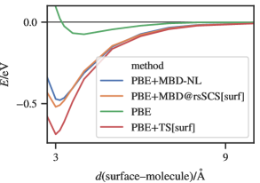
Figure 5: Binding energy of a single benzene molecule on a (111) silver surface.

Figure 5 compares the binding energy curve of a hybrid organic/inorganic interface as calculated by PBE-NL and surface variants of the MBD@rsSCS and TS methods by Ruiz et al. (2016).

Table 2: Timing of DFT and MBD calculations

	CPU timea [s]
Calculation	MoS2b	4a @ S12Lc
Complete KS-DFT	$3700$	$39\,000$
Single KS-DFT cycle	$250$	$1900$
Kinetic energy density	$120$	$31$
MBD energy	$0.6$	$1.2$

^aTotal single-core CPU time on an Intel Xeon Gold 6148 processor (Skylake). ^b6 atoms in a unit cell, 200 $k$-points. ^c148 atoms.

Table 2 presents timings of illustrative DFT+MBD calculations and their individual components for a simple inorganic material and a large organic complex. In both cases, the evaluation of the MBD energy is only a small fraction of the cost of the DFT calculation, even when the evaluation of the kinetic energy density needed for parametrization of MBD-NL is included in the cost of the MBD calculation.

The function $g(I,\chi)$ from eq. (6) of the main text is visualized in Figure 6.

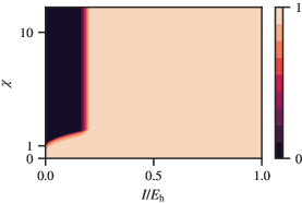
Figure 6: Smooth cutoff function for the low-gradient contributions to the polarizability.

References

- Adamo and Barone (1999) C. Adamo and V. Barone. Toward reliable density functional methods without adjustable parameters: The PBE0 model. J. Chem. Phys., 110:6158–6170, 1999. doi:10.1063/1.478522.
- Ambrosetti et al. (2014a) A. Ambrosetti, D. Alfè, R. A. DiStasio, Jr., and A. Tkatchenko. Hard Numbers for Large Molecules: Toward Exact Energetics for Supramolecular Systems. J. Phys. Chem. Lett., 5:849–855, 2014a. doi:10.1021/jz402663k.
- Ambrosetti et al. (2014b) A. Ambrosetti, A. M. Reilly, R. A. DiStasio, Jr., and A. Tkatchenko. Long-range correlation energy calculated from coupled atomic response functions. J. Chem. Phys., 140:18A508, 2014b. doi:10.1063/1.4865104.
- Becke and Edgecombe (1990) A. D. Becke and K. E. Edgecombe. A simple measure of electron localization in atomic and molecular systems. J. Chem. Phys., 92:5397–5403, 1990. doi:10.1063/1.458517.
- Becke and Johnson (2007) A. D. Becke and E. R. Johnson. Exchange-hole dipole moment and the dispersion interaction revisited. J. Chem. Phys., 127:154108, 2007. doi:10.1063/1.2795701.
- Björkman (2012) T. Björkman. Van der Waals density functional for solids. Phys. Rev. B, 86:165109, 2012. doi:10.1103/PhysRevB.86.165109.
- Björkman et al. (2012) T. Björkman, A. Gulans, A. V. Krasheninnikov, and R. M. Nieminen. Van der Waals Bonding in Layered Compounds from Advanced Density-Functional First-Principles Calculations. Phys. Rev. Lett., 108:235502, 2012. doi:10.1103/PhysRevLett.108.235502.
- Blum et al. (2009) V. Blum, R. Gehrke, F. Hanke, P. Havu, V. Havu, X. Ren, K. Reuter, and M. Scheffler. Ab initio molecular simulations with numeric atom-centered orbitals. Comput. Phys. Commun., 180:2175–2196, 2009. doi:10.1016/j.cpc.2009.06.022.
- Caldeweyher et al. (2019) E. Caldeweyher, S. Ehlert, A. Hansen, H. Neugebauer, S. Spicher, C. Bannwarth, and S. Grimme. A generally applicable atomic-charge dependent London dispersion correction. J. Chem. Phys., 150:154122, 2019. doi:10.1063/1.5090222.
- Dion et al. (2004) M. Dion, H. Rydberg, E. Schröder, D. C. Langreth, and B. I. Lundqvist. Van der Waals density functional for general geometries. Phys. Rev. Lett., 92:246401, 2004. doi:10.1103/PhysRevLett.92.246401.
- Dobson (2014) J. F. Dobson. Beyond pairwise additivity in London dispersion interactions. Int. J. Quantum Chem., 114:1157–1161, 2014. doi:10.1002/qua.24635.
- Fedorov et al. (2018) D. V. Fedorov, M. Sadhukhan, M. Stöhr, and A. Tkatchenko. Quantum-Mechanical Relation between Atomic Dipole Polarizability and the van der Waals Radius. Phys. Rev. Lett., 121:183401, 2018. doi:10.1103/PhysRevLett.121.183401.
- Ferri et al. (2015) N. Ferri, R. A. DiStasio, Jr., A. Ambrosetti, R. Car, and A. Tkatchenko. Electronic Properties of Molecules and Surfaces with a Self-Consistent Interatomic van der Waals Density Functional. Phys. Rev. Lett., 114:176802, 2015. doi:10.1103/PhysRevLett.114.176802.
- Gould et al. (2016) T. Gould, S. Lebègue, J. G. Ángyán, and T. Bučko. A Fractionally Ionic Approach to Polarizability and van der Waals Many-Body Dispersion Calculations. J. Chem. Theory Comput., 12:5920–5930, 2016. doi:10.1021/acs.jctc.6b00925.
- Grimme (2012) S. Grimme. Supramolecular Binding Thermodynamics by Dispersion-Corrected Density Functional Theory. Chem. Eur. J., 18:9955–9964, 2012. doi:10.1002/chem.201200497.
- Grimme et al. (2010) S. Grimme, J. Antony, S. Ehrlich, and H. Krieg. A consistent and accurate ab initio parametrization of density functional dispersion correction (DFT-D) for the 94 elements H-Pu. J. Chem. Phys., 132:154104, 2010. doi:10.1063/1.3382344.
- Grimme et al. (2016) S. Grimme, A. Hansen, J. G. Brandenburg, and C. Bannwarth. Dispersion-Corrected Mean-Field Electronic Structure Methods. Chem. Rev., 116:5105–5154, 2016. doi:10.1021/acs.chemrev.5b00533.
- Gutle et al. (1999) C. Gutle, A. Savin, J. B. Krieger, and J. Chen. Correlation energy contributions from low-lying states to density functionals based on an electron gas with a gap. Int. J. Quantum Chem., 75:885–888, 1999. doi:10.1002/(SICI)1097-461X(1999)75:4/5<885::AID-QUA53>3.0.CO;2-F.
- Hermann (2019a) J. Hermann. 2019a. doi:10.6084/m9.figshare.9943361.v2. Code as git repository.
- Hermann (2019b) J. Hermann. 2019b. doi:10.6084/m9.figshare.9943301.v1. Data in HDF5 format.
- Hermann (2019c) J. Hermann. Libmbd. 2019c. doi:10.5281/zenodo.3474093. Code as git repository.
- Hermann and Tkatchenko (2018) J. Hermann and A. Tkatchenko. Electronic exchange and correlation in van der Waals systems: Balancing semilocal and nonlocal energy contributions. J. Chem. Theory Comput., 14:1361–1369, 2018. doi:10.1021/acs.jctc.7b01172.
- Hermann et al. (2017) J. Hermann, R. A. DiStasio, Jr., and A. Tkatchenko. First-principles models for van der Waals interactions in molecules and materials: Concepts, theory, and applications. Chem. Rev., 117:4714–4758, 2017. doi:10.1021/acs.chemrev.6b00446.
- Hirshfeld (1977) F. L. Hirshfeld. Bonded-atom fragments for describing molecular charge densities. Theor. Chim. Acta, 44:129–138, 1977. doi:10.1007/BF00549096.
- Jaffe (2005) R. L. Jaffe. Casimir effect and the quantum vacuum. Phys. Rev. D, 72:021301(R), 2005. doi:10.1103/PhysRevD.72.021301.
- Kim et al. (2020) M. Kim, W. J. Kim, T. Gould, E. K. Lee, S. Lebègue, and H. Kim. uMBD: A Materials-Ready Dispersion Correction That Uniformly Treats Metallic, Ionic, and van der Waals Bonding. J. Am. Chem. Soc., 142:2346–2354, 2020. doi:10.1021/jacs.9b11589.
- Klimeš and Michaelides (2012) J. Klimeš and A. Michaelides. Perspective: Advances and challenges in treating van der Waals dispersion forces in density functional theory. J. Chem. Phys., 137:120901, 2012. doi:10.1063/1.4754130.
- Kümmel and Perdew (2003) S. Kümmel and J. P. Perdew. Two avenues to self-interaction correction within Kohn–Sham theory: Unitary invariance is the shortcut. Mol. Phys., 101:1363–1368, 2003. doi:10.1080/0026897031000094506.
- London (1930) F. London. Zur Theorie und Systematik der Molekularkräfte [On theory and classification of molecular forces]. Z. Physik, 63:245–279, 1930. doi:10.1007/BF01421741.
- Lu et al. (2009) D. Lu, Y. Li, D. Rocca, and G. Galli. Ab initio Calculation of van der Waals Bonded Molecular Crystals. Phys. Rev. Lett., 102:206411, 2009. doi:10.1103/PhysRevLett.102.206411.
- Lucas (1967) A. Lucas. Collective contributions to the long-range dipolar interaction in rare-gas crystals. Physica, 35:353–368, 1967. doi:10.1016/0031-8914(67)90184-X.
- McLachlan (1963) A. D. McLachlan. Retarded Dispersion Forces Between Molecules. Proc. Royal Soc. Lond. A, 271:387–401, 1963. doi:10.1098/rspa.1963.0025.
- Perdew et al. (1996) J. P. Perdew, K. Burke, and M. Ernzerhof. Generalized Gradient Approximation Made Simple. Phys. Rev. Lett., 77:3865–3868, 1996. doi:10.1103/PhysRevLett.77.3865.
- Reilly and Tkatchenko (2013) A. M. Reilly and A. Tkatchenko. Understanding the role of vibrations, exact exchange, and many-body van der Waals interactions in the cohesive properties of molecular crystals. J. Chem. Phys., 139:024705, 2013. doi:10.1063/1.4812819.
- Řezáč et al. (2011) J. Řezáč, K. E. Riley, and P. Hobza. S66: A Well-balanced Database of Benchmark Interaction Energies Relevant to Biomolecular Structures. J. Chem. Theory Comput., 7:2427–2438, 2011. doi:10.1021/ct2002946.
- Ruiz et al. (2012) V. G. Ruiz, W. Liu, E. Zojer, M. Scheffler, and A. Tkatchenko. Density-Functional Theory with Screened van der Waals Interactions for the Modeling of Hybrid Inorganic-Organic Systems. Phys. Rev. Lett., 108:146103, 2012. doi:10.1103/PhysRevLett.108.146103.
- Ruiz et al. (2016) V. G. Ruiz, W. Liu, and A. Tkatchenko. Density-functional theory with screened van der Waals interactions applied to atomic and molecular adsorbates on close-packed and non-close-packed surfaces. Phys. Rev. B, 93:035118, 2016. doi:10.1103/PhysRevB.93.035118.
- Sato and Nakai (2009) T. Sato and H. Nakai. Density functional method including weak interactions: Dispersion coefficients based on the local response approximation. J. Chem. Phys., 131:224104, 2009. doi:10.1063/1.3269802.
- Sato and Nakai (2010) T. Sato and H. Nakai. Local response dispersion method. II. Generalized multicenter interactions. J. Chem. Phys., 133:194101, 2010. doi:10.1063/1.3503040.
- Silvestrelli (2008) P. L. Silvestrelli. Van der Waals Interactions in DFT Made Easy by Wannier Functions. Phys. Rev. Lett., 100:053002, 2008. doi:10.1103/PhysRevLett.100.053002.
- Silvestrelli (2013) P. L. Silvestrelli. Van der Waals interactions in density functional theory by combining the quantum harmonic oscillator-model with localized Wannier functions. J. Chem. Phys., 139:054106, 2013. doi:10.1063/1.4816964.
- Sun et al. (2013) J. Sun, B. Xiao, Y. Fang, R. Haunschild, P. Hao, A. Ruzsinszky, G. I. Csonka, G. E. Scuseria, and J. P. Perdew. Density Functionals that Recognize Covalent, Metallic, and Weak Bonds. Phys. Rev. Lett., 111:106401, 2013. doi:10.1103/PhysRevLett.111.106401.
- Sun et al. (2015) J. Sun, A. Ruzsinszky, and J. P. Perdew. Strongly Constrained and Appropriately Normed Semilocal Density Functional. Phys. Rev. Lett., 115:036402, 2015. doi:10.1103/PhysRevLett.115.036402.
- Tkatchenko and Scheffler (2009) A. Tkatchenko and M. Scheffler. Accurate Molecular Van Der Waals Interactions from Ground-State Electron Density and Free-Atom Reference Data. Phys. Rev. Lett., 102:073005, 2009. doi:10.1103/PhysRevLett.102.073005.
- Tkatchenko et al. (2012) A. Tkatchenko, R. A. DiStasio, Jr., R. Car, and M. Scheffler. Accurate and Efficient Method for Many-Body van der Waals Interactions. Phys. Rev. Lett., 108:236402, 2012. doi:10.1103/PhysRevLett.108.236402.
- Tkatchenko et al. (2013) A. Tkatchenko, A. Ambrosetti, and R. A. DiStasio, Jr. Interatomic methods for the dispersion energy derived from the adiabatic connection fluctuation-dissipation theorem. J. Chem. Phys., 138:74106, 2013. doi:10.1063/1.4789814.
- Vydrov and Van Voorhis (2009) O. A. Vydrov and T. Van Voorhis. Nonlocal van der Waals Density Functional Made Simple. Phys. Rev. Lett., 103:063004, 2009. doi:10.1103/PhysRevLett.103.063004.
- Vydrov and Van Voorhis (2010a) O. A. Vydrov and T. Van Voorhis. Nonlocal van der Waals density functional: The simpler the better. J. Chem. Phys., 133:244103, 2010a. doi:10.1063/1.3521275.
- Vydrov and Van Voorhis (2010b) O. A. Vydrov and T. Van Voorhis. Dispersion interactions from a local polarizability model. Phys. Rev. A, 81:062708, 2010b. doi:10.1103/PhysRevA.81.062708.
- Yang et al. (2014) J. Yang, W. Hu, D. Usvyat, D. Matthews, M. Schütz, and G. K.-L. Chan. Ab initio determination of the crystalline benzene lattice energy to sub-kilojoule/mole accuracy. Science, 345:640–643, 2014. doi:10.1126/science.1254419.
- Zhang et al. (2018) G.-X. Zhang, A. M. Reilly, A. Tkatchenko, and M. Scheffler. Performance of various density-functional approximations for cohesive properties of 64 bulk solids. New J. Phys., 20:063020, 2018. doi:10.1088/1367-2630/aac7f0.