High-Dimensional Potential Energy Surfaces for Molecular Simulations

Abstract

An overview of computational methods to describe high-dimensional potential energy surfaces suitable for atomistic simulations is given. Particular emphasis is put on accuracy, computability, transferability and extensibility of the methods discussed. They include empirical force fields, representations based on reproducing kernels, using permutationally invariant polynomials, and neural network-learned representations and combinations thereof. Future directions and potential improvements are discussed primarily from a practical, application-oriented perspective.

1 Introduction

The dynamics of molecular (i.e. chemical, biological and physical) processes is governed by the underlying intermolecular interactions. These processes can span a wide range of temporal and spatial scales and make a characterization and the understanding of elementary processes at an atomistic scale a formidable task.¹ Examples for such processes are chemical reactions or functional motions in proteins. For typical organic reactions the time scales are on the order of seconds whereas the actual chemical step (i.e. bond breaking or bond formation) occurs on the femtosecond time scale. In other words, during $\sim 10^{15}$ vibrational periods energy is redistributed in the system until sufficient energy has accumulated along the preferred “progression coordinate” for the reaction to occur.² Similarly, the biological process of “allostery” couples two (or multiple) spatially separated binding sites of a protein which is used to regulate the affinity of certain substrates to a protein, thereby controlling metabolism.³ According to the conventional view of allostery, a conformational change of the protein (that might however be very small ⁴) is the source of a signal, but other mechanisms have been proposed as well which are based exclusively on structural dynamics⁵. Here, binding of a ligand at a so-called allosteric site increases (or decreases) the affinity for a substrate at a distant active site, and the process can span multiple time and spatial scales to the extent of the size of the protein itself. Hence, an allosteric protein can be viewed as a “transistor”, and complicated feedback networks of many such switches ultimately make up a living cell ⁶. As a third example, freezing and phase transitions in water are entirely governed by intermolecular interactions. Describing them at sufficient detail has been found extremely challenging and a complete understanding of the phase diagram or the structural dynamics of liquid water is still not available.

All the above situations require means to compute the total energy of the system computationally efficiently and accurately. The most accurate method is to solve the electronic Schrödinger equation for every configuration $\vec{x}$ of the system for which energies and forces are required. However, there are certain limitations which are due to the computational approach per se, e.g. the speed and efficiency of the method or due to practical aspects of quantum chemistry such as accounting for the basis set superposition error, the convergence of the Hartree-Fock wavefunction to the desired electronic state for arbitrary geometries, or the choice of a suitable active space irrespective of molecular geometry for problems with multi-reference character, to name a few. Improvements and future avenues for making QM-based approaches even more broadly applicable have been recently discussed.⁷ For problems that require extensive conformational sampling or sufficient statistics purely QM-based dynamics approaches are still impractical.

A promising use of QM-based methods are mixed quantum mechanics/molecular mechanics (QM/MM) treatments which are particularly popular for biophysical and biochemical applications.⁸ Here, the system is decomposed into a “reactive region” which is treated with a quantum chemical (or semiempirical) method and an environment described by an empirical force field. Such a decomposition considerably speeds up simulations such that even free energy simulations in multiple dimensions can be computed.⁹ One of the current open questions in such QM/MM simulations is that of the size of the QM region required for converged results which was recently considered for Catechol O-Methyltransferase.¹⁰

Other possibilities to provide energies for molecular systems are based on empirical energy expressions, fits of reference energies to reference data from quantum chemical calculations, representations of the energies by kernels or by using neural networks. These methods are the topic of the present perspective as they have shown to provide means to follow the dynamics of molecular systems over long time scales or to allow statistically significant sampling of the process of interest.

First, explicit representations of energy functions are discussed. This usually requires one to choose a functional form of the model function. Next, machine learned potential energy surfaces are discussed. In a second part, topical applications of these methods are presented.

2 Explicit Representations

Empirical force fields are one of the most seasoned concepts to represent the total energy of a molecular system given the coordinates $\vec{x}$ of all atoms. The general expression for an empirical FF includes bonded $E_{\rm bonded}$ and nonbonded $E_{\rm nonbonded}$ terms.

$$E(\bf x) = \sum_{\rm bonds}k_{b}(r-r_{e})^{2}+\sum_{\rm angle}k_{\theta}(\theta-\theta_{e})^{2}\sum_{\rm dihedrals}k_{\chi}(1+\cos{n\chi-\delta})+\sum_{\rm impropers}k_{imp}(\phi-\phi_{0})^{2}$$ (1)

$$+ \sum_{\rm nonbonded}\epsilon_{ij}\left[\left(\frac{R_{\rm min_{\rm ij}}}{r_{ij}}\right)^{12}-\left(\frac{R_{\rm min_{\rm ij}}}{r_{ij}}\right)^{12}\right]+\frac{q_{i}q_{j}}{\epsilon_{l}r_{ij}}$$

Such representations can be evaluated very efficiently, the forces are readily available and systems containing millions of atoms can be simulated for extended time scales. On the other hand, the accuracy of such force fields compared with high-level electronic structure methods is very limited. Conversely, one of the noteworthy advantages of empirical energy functions is that they can be consistently and incrementally improved. Examples include the replacement of harmonic potentials for chemical bonds by Morse oscillator functions or extending the point charge electrostatics through multipolar series expansions.^{11, 12, 13, 14} Also, additional terms can be included to provide a more physically motivated representation, such as adding a term for polarization interactions.¹⁵

For smaller molecular systems more accurate representations are possible. Typically, reference energies are computed from quantum chemical calculations on a grid (regular or irregular) of molecular geometries. These energies are then used to fit parameters in a predetermined functional form to minimize the difference between the reference energies and the model function.

One example for such a predefined functional form are permutationally invariant polynomials (PIPs) which have been applied to molecules with 4 to 10 atoms and to investigate diverse physico-chemical problems.¹⁶ Using PIPs, the permutational symmetry arising in many molecular systems is explicitly built into the construction of the parametrized form of the PES. The monomials are of the form $y_{ij}=\exp{\left(-r_{ij}/a\right)}$ where the $r_{ij}$ are atom-atom separations and $a$ is a range parameter. The total potential is then expanded into multinomials, i.e. products of monomials with suitable expansion coefficients. For an A₂B molecule the symmetrized basis is $y_{12}^{a}(y_{13}^{b}y_{23}^{c}+y_{23}^{b}y_{13}^{c})$ which explicitly obeys permutational symmetry. A library for constructing the necessary polynomial basis has been made publicly available. ¹⁷

One application of PIPs includes the dissociation reaction of CH${}_{5}^{+}$ to CH${}_{3}^{+}$ + H₂ for which more than 36000 energies¹⁸ were fitted with an accuracy of 78.1 cm^-1. With this PES the branching ratio to form HD and H₂ for CH₄D⁺ and CH${}_{5}^{+}$, respectively, was determined. Also, the infrared spectra of various isotopes were computed with this PES.¹⁹ Other applications concern a fitted energy function for water dimer,²⁰ which became the basis for the WHBB force field for liquid water²¹ and that for acetaldehyde.²² For acetaldehyde roughly 135’000 energies at the CCSD(T)/cc-pVTZ level of theory were fitted to 2655 terms with order 5 in the polynomial basis and 9953 terms with order 6 in the polynomial basis. For the relevant stationary states in that study the difference between the reference calculations and the fit ranges from 2 to 4.5 kcal/mol. However, the overall RMSD for all fitted points has not been reported.²² With this PES the fragment population for dissociation into CH₃ + HCO and CH₄ + CO was investigated.

Another fruitful approach are double many body expansions.²³ These decompose the total energy of a molecular system first into one- and several many-body terms and then represent each of them as a sum of short- and long-range contributions.²³ This yields, for example, an RMSD of 0.99 kcal/mol for 3701 fitted points from electronic structure calculations at the MRCI level of theory for CNO.²⁴ As a comparison, another recent investigation of the same system²⁵ using a reproducing kernel Hilbert space (RKHS, see further below) representation yielded an RMSD of 0.38, 0.48 and 0.47 kcal/mol for the ²A^′, ²A^′′ and ⁴A^′′ electronic states using more than 10000 ab initio points for each surface.

Local interpolation has also been shown to provide a meaningful approach. One such approach is Shepard interpolation which represents the PES as a weighted sum of force fields, expanded around several reference geometries.^{26, 27} Also, recently several computational resources have been made available to construct fully-dimensional PESs for polyatomic molecules such as Autosurf²⁸ or a repository to automatically construct PIPs.

3 Machine Learned PESs

Machine learning (ML) methods have become increasingly popular in recent years in order to construct PESs, or estimate other properties of unknown compounds or structures.^{29, 30, 31, 32} Such approaches give computers the ability to learn patterns in data without being explicitly programmed.³³ For PES construction, suitable reference data are e.g. energy, forces, or both, usually obtained from ab initio methods. Contrary to the explicit representations discussed in section 2, ML-based PESs are non-parametric and not limited to a predetermined functional form.

Most ML methods used for PES construction are either kernel-based or rely on artificial neural networks (ANNs). Both variants take advantage of the fact that many nonlinear problems (such as predicting energy from nuclear positions) can be linearised by mapping the inputs to a (often higher-dimensional) feature space (see Fig. 1).³⁴

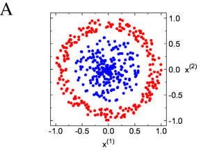
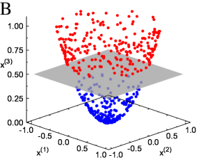
Figure 1: A: The blue and red points with coordinates ($x^{(1)}$ , $x^{(2)}$) are linearly inseparable. B: By defining a suitable mapping from the input space ($x^{(1)}$,$x^{(2)}$) to a higher-dimensional feature space ($x^{(1)}$,$x^{(2)}$;,$x^{(3)}$), blue and red points become linearly separable by a plane at $x^{(3)}=0.5$ (grey).

Kernel-based methods utilize the kernel trick,^{35, 36, 37} which allows to operate in an implicit feature space without explicitly computing the coordinates of data in that space (see section 3.1 for more details). ML methods based on ANNs rely on “neuron layers”, which map their inputs to feature spaces by linear transformations with learnable parameters, followed by a nonlinearity (called activation function). Often, many such layers are stacked on top of each other to build increasingly complex feature spaces (see section 3.2). In the following, both variants are discussed in more detail.

3.1 Reproducing Kernel Representations

Starting from a data set $\{(y_{i};\mathbf{x}_{i})\}_{i=1}^{N}$ of $N$ observations $y_{i}\in\mathbb{R}$ given the inputs $\mathbf{x}_{i}\in\mathbb{R}^{D}$, kernel regression aims to estimate unknown values $y_{*}$ for inputs $\mathbf{x}_{*}$. For a PES, $y$ is typically the total interaction energy and $\mathbf{x}$ is a representation of chemical structure (i.e. a vector of internal coordinates, a molecular descriptor like the Coulomb matrix²⁹, descriptors for atomic environments, e.g. symmetry functions³⁸, SOAP³⁹ or FCHL^{40, 41}, or a representation of crystal structure ^{42, 43, 44}). The representer theorem⁴⁵ for a functional relation $y=f(\mathbf{x})$ states that $f(\mathbf{x})$ can always be approximated as a linear combination

$$f(\mathbf{x})\approx\widetilde{f}(\mathbf{x})=\sum_{i=1}^{N}\alpha_{i}K(\mathbf{x},\mathbf{x}_{i})$$ (2)

where $\alpha_{i}$ are coefficients and $K(\mathbf{x},\mathbf{x^{\prime}})$ is a kernel function. A function $K(\mathbf{x},\mathbf{x^{\prime}})$ is a reproducing kernel of a Hilbert space $\mathcal{H}$ if the inner product $\langle\phi(\mathbf{x}),\phi(\mathbf{x^{\prime}})\rangle$ of $\mathcal{H}$ can be expressed as $K(\mathbf{x},\mathbf{x^{\prime}})$.⁴⁶ Here, $\phi$ is a mapping from the input space $\mathbb{R}^{D}$ to the Hilbert space $\mathcal{H}$, i.e. $\phi:\mathbb{R}^{D}\mapsto\mathcal{H}$. Many different kernel functions are possible, for example the polynomial kernel

$$K(\mathbf{x},\mathbf{x^{\prime}})=\langle\mathbf{x},\mathbf{x^{\prime}}\rangle^{d}$$ (3)

where $\langle\cdot,\cdot\rangle$ denotes the dot product and $d$ is the degree of the polynomial, or the Gaussian kernel given by

$$K(\mathbf{x},\mathbf{x^{\prime}})=e^{-\gamma\lVert\mathbf{x}-\mathbf{x^{\prime}}\rVert^{2}}$$ (4)

are popular choices. Here, $\gamma$ is a hyperparameter determining the width of the Gaussian and $\lVert\cdot\rVert$ denotes the $L^{2}$-norm. It is also possible to include knowledge about the long range behaviour of the physical interactions into the kernel function itself⁴⁷ and the consequences of such choices on the long- and short-range behaviour of the inter- and extrapolation have been investigated in quite some detail.⁴⁸

The mapping $\phi$ associated with the polynomial kernel (Eq. 3) depends on the dimensionality of the inputs $\mathbf{x}$ and the chosen degree $d$ of the kernel. For example, for $d=2$ and two-dimensional input vectors, the mapping is given by $\phi:(x_{1},x_{2})\mapsto(x_{1}^{2},\sqrt{2}x_{1}x_{2},x_{2}^{2})$ and the Hilbert space $\mathcal{H}$ associated with the kernel function is three-dimensional. For a Gaussian kernel, the associated Hilbert space $\mathcal{H}$ even is $\infty$-dimensional. This can easily be seen if Eq. 4 is rewritten as

$$K(\mathbf{x},\mathbf{x^{\prime}})=e^{-\gamma\lVert\mathbf{x}\rVert^{2}}e^{-\gamma\lVert\mathbf{x^{\prime}}\rVert^{2}}e^{2\gamma\langle\mathbf{x},\mathbf{x^{\prime}}\rangle}$$ (5)

then the Taylor expansion of the third factor $e^{2\gamma\langle\mathbf{x},\mathbf{x^{\prime}}\rangle}=\sum_{d=0}^{\infty}\frac{1}{d!}\left(2\gamma\langle\mathbf{x},\mathbf{x^{\prime}}\rangle\right)^{d}$ reveals that the Gaussian kernel is equivalent to an infinite sum over polynomial kernels (scaled by constant terms). It is important to point out that in order to apply Eq. 2, the mapping $\phi$ has never to be calculated explicitly (or even known at all) and it is therefore possible to operate in the (high-dimensional) space $\mathcal{H}$ implicitly. This is often referred to as the kernel trick^{35, 36, 37}.

The coefficients $\alpha_{i}$ (Eq. 2) can be determined such that $\widetilde{f}(\mathbf{x}_{i})=y_{i}$ for all inputs $\mathbf{x}_{i}$ in the dataset, i.e.

$$\boldsymbol{\alpha}=\mathbf{K}^{-1}\mathbf{y}$$ (6)

where $\boldsymbol{\alpha}=\left[\alpha_{i}\cdots\alpha_{N}\right]^{\mathrm{T}}$ is the vector of coefficients, $\mathbf{K}$ is an $N\times N$ matrix with entries $K_{ij}=K(\mathbf{x}_{i},\mathbf{x}_{j})$ called kernel matrix^{49, 50} and $\mathbf{y}=\left[y_{1}\cdots y_{N}\right]^{\mathrm{T}}$ is a vector containing the $N$ observations $y_{i}$ in the data set. Since the kernel matrix is symmetric and positive-definite by construction, the efficient Cholesky decomposition⁵¹ can be used to solve Eq. 6. Once the coefficients $\alpha_{i}$ have been determined, unknown values $y_{*}$ at arbitrary positions $\mathbf{x}_{*}$ can be estimated as $y_{*}=\widetilde{f}(\mathbf{x}_{*})$ using Eq. 2.

In practice however, the solution of Eq. 6 is only possible if the kernel matrix $\mathbf{K}$ is well-conditioned. Fortunately, in case $\mathbf{K}$ is ill-conditioned, a regularized solution can be obtained for example by Tikhonov regularization⁵². This amounts to adding a small positive constant $\lambda$ to the diagonal of $\mathbf{K}$, such that

$$\boldsymbol{\alpha}=\left(\mathbf{K}+\lambda\mathbf{I}\right)^{-1}\mathbf{y}$$ (7)

is solved instead of Eq. 6 when determining the coefficients $\alpha_{i}$ (here, $\mathbf{I}$ is the identity matrix). For non-zero $\lambda$ however, $\widetilde{f}(\mathbf{x}_{i})\neq y_{i}$ and Eq. 2 reproduces the known values in the data set only approximately. Therefore, this method of determining the coefficients can also be used to prevent over-fitting and is known as kernel ridge regression (KRR).⁵³

KRR is closely related to Gaussian process regression (GPR).⁵⁴ In GPR, it is assumed that the $N$ observations $\{(y_{i};\mathbf{x}_{i})\}_{i=1}^{N}$ in the data set are generated by a Gaussian process, i.e. drawn from a multivariate Gaussian distribution with zero mean, and covariance $K(\mathbf{x},\mathbf{x^{\prime}})$. Note that a mean of zero can always be assumed without loss of generality since two multivariate Gaussian distributions with equal covariance matrix can always be transformed into each other by addition of a constant term. Further, every observation $y_{i}$ is considered to be related to $\mathbf{x}_{i}$ through an underlying function $f(\mathbf{x})$ and some observational noise (e.g. due to uncertainties in measuring $y_{i}$)

$$y_{i}=f(\mathbf{x}_{i})+\mathcal{N}(0,\lambda)$$ (8)

where $\lambda$ is the variance of the Gaussian noise model. The chosen covariance function $K(\mathbf{x},\mathbf{x^{\prime}})$ expresses an assumption about the nature of $f(\mathbf{x})$. For example, if the Gaussian kernel (Eq. 4) is used, $f(\mathbf{x})$ is assumed to be smooth and the chosen Gaussian width $\gamma$ determines how rapid $f(\mathbf{x})$ is allowed to change if the input $\mathbf{x}$ changes.

With these assumptions, it is now possible to determine the conditional probability $p(y_{*}|\mathbf{y})$, i.e. answer the question “given the data $\mathbf{y}=\left[y_{1}\cdots y_{N}\right]^{\mathrm{T}}$, how likely is it to observe the value $y_{*}$ for an input $\mathbf{x}_{*}$?”. Since it was assumed that the data was drawn from a multivariate Gaussian distribution, it is possible to write

$$\begin{bmatrix}\mathbf{y}\textbf{}\\ y^{*}\end{bmatrix}\sim\mathcal{N}\left(0,\begin{bmatrix}\mathbf{K}+\lambda\mathbf{I}&\mathbf{K}_{*}^{\mathrm{T}}\\ \mathbf{K}_{*}&K(\mathbf{x}_{*},\mathbf{x}_{*})\end{bmatrix}\right)$$ (9)

where $\mathbf{K}$ is the kernel matrix (see Eq. 6) and $\mathbf{K}_{*}=\left[K(\mathbf{x}_{*},\mathbf{x}_{1})\cdots K(\mathbf{x}_{*},\mathbf{x}_{N})\right]$. Then, the best (most likely) estimate for $y_{*}$ is the mean of this distribution

$$\bar{y}_{*}=\mathbf{K}_{*}\left(\mathbf{K}+\lambda\mathbf{I}\right)^{-1}\mathbf{y}$$ (10)

Thus, estimating $y_{*}$ with GPR (Eq. 10) is mathematically equivalent to estimating $y_{*}$ with KRR (compare to Eqs. 2 and 7). However, while in KRR, $\lambda$ is only a hyperparameter related to regularization, in GPR, $\lambda$ is directly related to the magnitude of the assumed observational noise (see Eq. 8). Further, the predictive variance,

$$\mathrm{var}(y_{*})=K(\mathbf{x}_{*},\mathbf{x}_{*})-\mathbf{K}_{*}\left(\mathbf{K}+\lambda\mathbf{I}\right)^{-1}\mathbf{K}_{*}^{\mathrm{T}}$$ (11)

which can also be derived from Eq. 9, can be useful to estimate the uncertainty of a prediction $y_{*}$, i.e. how confident the model is that its prediction is correct. Since KRR and GPR are so similar, they are both referred to as reproducing kernel representations in this work.

3.2 Artificial Neural Networks

The basic building blocks of artificial neural networks (NNs)^{55, 56, 57, 58, 59, 60, 61} are so-called “dense (neuron) layers”, which transform input vectors $\mathbf{x}\in\mathbb{R}^{n_{\rm in}}$ linearly to output vectors $\mathbf{y}\in\mathbb{R}^{n_{\rm out}}$ through

$$\mathbf{y}=\mathbf{W}\mathbf{x}+\mathbf{b}$$ (12)

where the weights $\mathbf{W}\in\mathbb{R}^{n_{\rm out}\times n_{\rm in}}$ and biases $\mathbf{b}\in\mathbb{R}^{n_{\rm out}}$ are parameters, and $n_{\rm in}$ and $n_{\rm out}$ denote the dimensionality of inputs and outputs, respectively. A single dense layer can therefore only represent linear relations. To model non-linear relationships between inputs and outputs, at least two dense layers need to be combined with a non-linear function $\sigma$ (called activation function), i.e.

$$\mathbf{h}= \sigma\left(\mathbf{W}_{1}\mathbf{x}+\mathbf{b}_{1}\right)$$ (13)

$$\mathbf{y}= \mathbf{W}_{2}\mathbf{h}+\mathbf{b}_{2}$$ (14)

Such an arrangement (Eqs. 13 and 14) has been proven to be a general function approximator, meaning that any mapping between input $\mathbf{x}$ and output $\mathbf{y}$ can be approximated to arbitrary precision, provided that the dimensionality of the so-called “hidden layer” $\mathbf{h}$ is large enough.^{62, 63} As such, NNs are a natural choice for representing a PES, i.e. a mapping from chemical structure to energy (for PES construction, the output $\mathbf{y}$ usually is one-dimensional and represents the energy).

While shallow NNs with a single hidden layer (see above) are in principle sufficient to solve any learning task, in practice, deep NNs with multiple hidden layers are exponentially more parameter-efficient.⁶⁴ In a deep NN, $l$ hidden layers are stacked on top of each other,

$$\mathbf{h}_{1} =\sigma\left(\mathbf{W}_{1}\mathbf{x}+\mathbf{b}_{1}\right)$$ (15)

$$\mathbf{h}_{2} =\sigma\left(\mathbf{W}_{2}\mathbf{h}_{1}+\mathbf{b}_{2}\right)$$

$$\vdots$$

$$\mathbf{h}_{l} =\sigma\left(\mathbf{W}_{l}\mathbf{h}_{l-1}+\mathbf{b}_{l}\right)$$

$$\mathbf{y} =\mathbf{W}_{l+1}\mathbf{h}_{l}+\mathbf{b}_{l+1}$$

mapping the inputs $\mathbf{x}$ to increasingly complex feature spaces, until the features $\mathbf{h}_{l}$ in the final layer are linearly related to the outputs $\mathbf{y}$. The parameters of the NN, i.e. the entries in the matrices $\mathbf{W}_{l}$ and vectors $\mathbf{b}_{l}$, are initialized randomly and then optimized, for example via gradient descent, to minimize a loss function that measures the difference between the output of the NN and a given set of training data. For example, the mean squared error (MSE) is a popular loss function for regression tasks.

The earliest NN-based PESs directly use a set of internal coordinates, e.g. distances and angles, as input for the NN.^{65, 66, 67, 68, 69} However, such approaches have the disadvantage that swapping symmetry equivalent atoms may also change the numeric values of the internal coordinates. Since it is not guaranteed that a NN maps two different inputs related by a permutation operation to the same output energy, the permutational invariance of the PES is violated. Another disadvantage of using internal coordinates as input is that a NN trained for a single molecule cannot be used to calculate the energy of a dimer, because they require a different number of internal coordinates for an unambiguous description of the molecular geometry. Therefore, for small systems, PESs based on NNs have been designed in the spirit of a many-body expansion,^{70, 71, 72} which circumvents these issues. However, these approaches involve a large number of individual NNs, i.e. one for each term in the many-body expansion and scale poorly for large systems.

For larger systems, it is common practice to decompose the total energy of a chemical system into atomic contributions, which are predicted by a single NN (or one for each element). This approach, known as high-dimensional neural network (HDNN)⁷³ and first proposed by Behler and Parrinello, relies on the chemically intuitive assumption that the contribution of an atom to the total energy depends mainly on its local environment.

Two variants of HDNNs can be distinguished: The “descriptor-based” variant uses a hand-crafted descriptor,^{38, 74, 75, 76} to encode the environment of an atom, which is then used as input of a multi-layer feed-forward NN. Examples for this kind of approach are ANI⁷⁷ and TensorMol.⁷⁸ The “message-passing”⁷⁹ variant directly uses nuclear charges and Cartesian coordinates as input and a deep neural network (DNN) is used to exchange information (“messages”) between individual atoms, such that a representation of their chemical environments is learned directly from the data. The DTNN⁸⁰ introduced by Schütt et al. was the first NN of this kind and has since been refined in other DNN architectures, for example SchNet⁸¹, HIP-NN⁸² or PhysNet⁸³. Both types of HDNN perform well, however, the message-passing variant is able to automatically adapt the description of the chemical environments to the training data and the prediction task at hand and usually achieves a better performance.⁸⁴

4 Applications

In the following, illustrative applications of explicit representations of PESs (see section 2) and machine-learned PESs (see section 3) are discussed. Potential energy surfaces of sufficient quality for gas- and solution-phase reactions differ in at least two respects. While for reactions in the gas phase, typically involving small molecules as reactants, techniques to construct global, reactive PESs are becoming available, this is not so for reactions in solutions. Often, the global property is also not required a priori for reactions in solution. Secondly, for reactions in the gas phase all interactions are typically encoded in the global, reactive PES itself, whereas for reactions in solution the interaction between solute and solvent needs to be represented separately and explicitly. Therefore gas- and solution-phase are discussed in two different sections  4.1 and 4.2. While PESs are often used to explore the conformational space of a given system or study molecular (reaction) dynamics, machine-learned PESs can also serve as an alternative to ab initio methods for exploring chemical compound space. For example, it is possible to predict energies of molecules of different chemical composition from learning on a reference data set. Such applications are discussed briefly in section 4.3.

4.1 Gas Phase Reaction Dynamics

Multisurface, reactive dynamics for triatomics:

Triatomic systems constitute an important class of systems relevant to the chemistry in the hypersonic regime. Typical reactive collisions upon reentry of objects from outer space into Earth’s atmosphere include the O+NO, O+CO, N+CO, C+NO, or N+NO systems. Due to the high velocities of the impacting object, temperatures up to 20000 K can be reached. To study the reaction dynamics at such high collision energies both, ground and lower electronically excited states need to be included. Hence, to describe the reactive dynamics for such systems, fully dimensional, reactive PESs including multiple electronic states are required. This is possible by using a large number of ab initio calculated energies at the multi-reference CI level of theory and representing the PESs using a reproducing kernel Hilbert space (RKHS). Alternative approaches use explicit fitting of a parametrized form of a suitable many body expansion of the PES.²³

One example for such a system constitutes the reactive dynamics of [CNO] in the hypersonic regime at temperatures up to $T=20000$ K.²⁵ The C+NO reaction is important in combustion chemistry and NO plays a crucial role in the chemistry near the surface of a space vehicle during atmospheric re-entry.⁸⁵ For this, accurate fully dimensional PESs for the ²A^′, ²A^′′ and ⁴A^′′ states were determined and used in quantum dynamics and quasiclassical trajectory simulations. More than 50000 ab initio energies were calculated at the MRCI+Q/aug-cc-pVTZ level of theory to construct the RKHS PESs. The electronic structure calculations were performed in grids based on Jacobi coordinates for each channels. RKHS was used to construct analytical representations for each channel and global 3D PES was then made by smoothly connecting the PESs for the three channels by switching functions. Correlation plots of the MRCI+Q energies and the analytical energies obtained from the 3D RKHS based PESs are shown in Figure 2 for three sets of off-grid points calculated to validate the quality of the RKHS-based global PESs. RKHS energies for different 1D cuts are compared with ab initio energies in all three channels for the ²A^′′ PES in Figure 3. The contour plots shown in Figure 3 shows the topology of the ²A^′ PES for all three channels. The overall good agreement between the ab initio and analytical energies in all the channels and for all the electronic states suggests the high quality of the PESs.

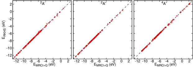
Figure 2: Correlation between the RKHS and MRCI+Q energies for test data set for ²A^′, ²A^′′ and ⁴A^′′ electronic state of CNO system. Black dashed line shows the diagonal. Data taken form Ref. ²⁵

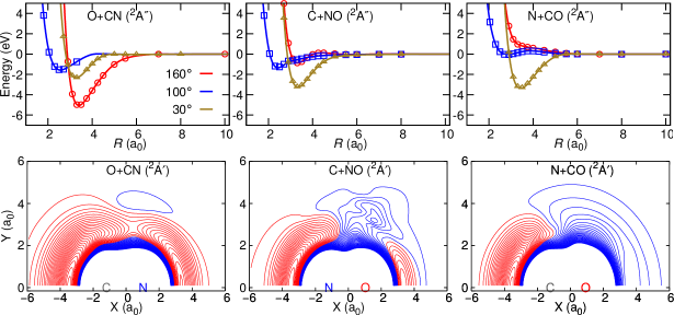
Figure 3: Upper panel: Comparison between the RKHS (solid lines) and MRCI+Q (open symbols) energies for different 1D cuts in Jacobi coordinates in the O+CN, C+NO and N+CO channels for the ²A^′′ electronic state of CNO system. Lower panel: Contour diagram of the 3D RKHS PESs for three different channels of CNO ²A^′ system. The diatoms are fixed to their equilibrium geometry and the zero is set to the asymptotic value for each channels. Data taken form Ref. ²⁵

Experimental reference data is available for the rate coefficients and branching fractions of CO and CN products for the the C(³P) + NO(X${}^{2}\Pi$) $\rightarrow$ O(³P) + CN(X${}^{2}\Sigma^{+}$) and N(²D)/N(⁴S) + CO(X${}^{1}\Sigma^{+}$) reaction.^{86, 87, 88} From 40000 QCT trajectories at each temperature on each PES run both, in an adiabatic and a nonadiabatic fashion within a Landau-Zener^{89, 90, 91, 92} formalism, the rate coefficients and branching fractions were determined. These rates can be directly compared with experiments and previous simulations. Figure 4 shows the rate coefficients and branching ratios for the products. Except for the lowest temperatures ($T\sim 30$ K and below) the rate coefficients agree well with experiments. Furthermore, it was found that including nonadiabatic transitions leads to better agreement with experiment within error bars but without nonadiabatic transitions the branching fractions were underestimated, see right panel in Figure 4. In addition, computed final state distributions of the products for molecular beam-type simulations agree well with experiment. From such studies, thermal rates within an Arrhenius formalism can be determined which can then be used in more coarse grained simulations, such as discrete sampling Monte Carlo (DSMC).⁹³

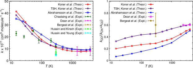
Figure 4: Total rate coefficients (left) and branching fractions (right) C(³P) + NO(X${}^{2}\Pi$) $\rightarrow$ O(³P) + CN(X${}^{2}\Sigma^{+}$) and N(²D)/N(⁴S) + CO(X${}^{1}\Sigma^{+}$) reaction compared with available experimental and theoretical data. Data taken form Ref. ²⁵

Reactive dynamics of larger gas-phase systems:

One recent application of MS-ARMD and a NN-trained PES concerned the Diels-Alder reaction between 2,3-dibromo-1,3-butadiene (DBB) and maleic anhydride (MA).⁹⁴ DBB is a generic diene which fulfills the experimental requirements for conformational separation of its isomers by electrostatic deflection of a molecular beam,^{95, 96} thus enabling the characterization of conformational aspects and specificities of the reaction. MA is a widely used, activated dienophile which due to its symmetry simplifies the possible products of the reaction. The reaction of DBB and MA thus serves as a prototypical system well suited for the exploration of general mechanistic aspects of Diels-Alder processes in the gas phase. The main questions concerned the synchronicity and concertedness of the reaction and how the reaction could be promoted. Until now, computational studies of Diels-Alder reactions including the molecular dynamics have started from TS-like structures^{97, 98, 99, 100, 101} or have used steered dynamics¹⁰² both of which introduce biases and do not allow direct calculation of reaction rates.

To do so, two different reactive PESs were developed. One was based on the MS-ARMD approach whereas the second one employed the PhysNet⁸³ architecture to train a NN representation. For both representations scattering calculations were started from suitable initial conditions by sampling the internal degrees of freedom of the reactants and the collision parameter $b$. It is found that the majority of reactive collisions occur with rotational excitation and that most of them are synchronous. The relevance of rotational degrees of freedom to promote the reaction was also found when the minimum dynamical path¹⁰³ was calculated. The dynamics on both, the MS-ARMD and NN-trained PESs are very similar although the quality of the two surfaces is different. While the NN-trained PES is able to reproduce the training data to within 0.25 kcal/mol on average, the RMSD between reference and parametrized PES for MS-ARMD is 1.5 kcal/mol over a range of 80 kcal/mol. In terms of computational efficiency MS-ARMD is about 200 times faster than PhysNet.

Another prototypical example of a chemical reaction is the S_N2 mechanism. In a recent comparative study,¹⁰⁴ three reactive PESs for the [Cl–CH₃–Br]^- system were constructed: Two of these PESs rely on empirical force fields, either combined with the MS-ARMD or the MS-VALBOND¹⁰⁵ approach to construct the global reactive PES, whereas the third is NN-based. While all methods are able to fit the ab initio reference data with $R^{2}>0.99$, the NN-based PES achieves mean absolute and root mean squared deviations that are an order of magnitude lower than the other methods when using the same number of reference data. When increasing the size of the reference data set, the prediction errors made by the NN-based PES are even up to three orders of magnitude lower than for the force field-based PESs. However, at the same time, evaluating the NN-based PES is about three orders of magnitude slower.¹⁰⁴

4.2 Reactions in the Condensed Phase

For reactions in the condensed phase, two different situations are considered in the following. In one of them, ligands bind to a substrate anchored within a protein, such as for small diatomic ligands binding to the heme-group in globins. In the other, the substrate is chemically transformed as is the case for the Claisen rearrangement from chorismate to prephenate.

Ligand (Re-)Binding in Globins:

Computationally, the structural dynamics accompanying NO-rebinding to Myoglobin has recently been investigated with the aim to assign the transient, metastable structures relevant for rebinding of the ligand on different time scales.¹⁰⁶ For this, reactive MD simulations using MS-ARMD simulations were run involving the bound ${}^{2}A$ and the unbound ${}^{4}A$ states which are also probed experimentally. The energy for each of the states was represented as a reproducing kernel^{106, 47, 107} for the subspace of important system coordinates (the heme(Fe)–NO separation and angle, and the doming coordinate of the heme-Fe) combined with an empirical force field for all remaining degrees of freedom. Such an approach is inspired by a decomposition of the system into a region that is modelled with high accuracy (typically a “quantum region”) and an environment (the “molecular mechanics” part).

With a system parametrized in this fashion, extensive reactive MD simulations were run.¹⁰⁶ The kinetics for ligand rebinding is nonexponential with time scales of 10 and 100 ps. These are consistent with time scales measured from optical, infrared, and X-ray absorption experiments and previous computational work.^{108, 109, 110, 111, 112, 113, 114, 115, 116, 117, 118, 119} The influence of the iron-out-of-plane (Fe-oop or “doming”) coordinate on the rebinding reaction, as predicted by experiment¹¹¹, was directly established. The two time scales (10 and 100 ps) are associated with two structurally different states of the His64 side chain – one “out” (state A) and one “in” (state B) – which control ligand access and rebinding dynamics. Such an unequivocal assignment was not possible from experiment.¹²⁰ In addition, the simulations provide an explanation why an energetically feasible state for NO-binding to heme is typically not found in Mb: Although the bound Fe-ON state is a local minimum on the potential energy surface, the energy of this state on the unbound ${}^{4}A$ manifold is lower and, hence, the bound ${}^{2}A$ Fe-ON can not be spectroscopically characterized. The simulations finally clarify that the XAS experiments are unable to distinguish between structures with photodissociated NO “close to” or “far away” from the heme-Fe in the active site as had been proposed.¹¹⁴

In this fashion, validation of experimental results by the MD simulations and in-depth analysis of the configurations driving the dynamics on the different time scales (10 ps and 100 ps) allowed to identify the structural origins of the conformational dynamics at a molecular level. It is expected that further combined experimental and computational studies of this kind will provide the necessary insight to link energetics, structures and dynamics in complex systems.

Reactions in Solution:

The Claisen rearrangement¹²¹ is an important [3,3]-sigmatropic rearrangement for high stereoselective¹²² C-C bond formation¹²³. The text book example of a Claisen rearrangement is the reaction of allyl-vinyl ether (AVE) to pent-4-enal¹²⁴. In polar solvent the stabilization of the transition state (TS) relative to the reaction in vacuum is the origin of the catalytic effect.^{125, 126, 127} This has motivated numerous studies on enzymatic Claisen rearrangements in particular^{128, 129, 130, 131, 132, 133, 134, 135, 136, 137, 138} and reactions with related substrates^{139, 140, 141, 142}. Compared to the reaction in aqueous solution the enzymatic catalysis of the Claisen rearrangement reaction in chorismate mutase (CM) leads to a rate acceleration by $\sim 10^{6}$ due to stabilisation of the TS.¹⁴³

A reactive force field based on MS-ARMD was parametrized for AVE and used unchanged for AVE-(CO₂)₂ and chorismate to study their Claisen rearrangements in the gas phase, in water and in the chorismate mutase from Bacillus subtilis (BsCM). Using free energy simulations it is found that in going from AVE and AVE-(CO₂)₂ to chorismate and using the same reactive PES the rate slows down when going from water to the protein as the environment. However, for the largest substrate (chorismate) they correctly find that the protein accelerates the reaction. Considering the changes of $+4.6$ (AVE), $+2.9$ (AVE-(CO₂)₂) and $-4.4$ (chorismate) kcal/mol in the activation free energies and correlating them with the actual chemical modifications suggests that both, electrostatic stabilization (AVE$\rightarrow$AVE-(CO${}_{2})_{2}$) and entropic contributions (AVE-(CO₂)${}_{2}\rightarrow$ chorismate, through the rigidification and larger size of chorismate) lead to the rate enhancement observed for chorismate in CM.

As for the reaction itself it is found that for all substrates considered the O-C bond breaks prior to C-C bond formation. This agrees with kinetic isotope experiments according to which C-O cleavage always precedes C-C bond formation.¹⁴⁴ For the nonenzymatic thermal rearrangement of chorismate to prephenate the measured kinetic isotope effects^{145, 144} indicate that at the TS the C-O bond is about 40 % broken but little or no C-C bond is formed, consistent with an analysis based on “More O’Ferrall-Jencks” (MOFJ) diagrams.^{146, 147}

The analysis of the TS position in the active site of BsCM reveals that the lack of catalytic effect on AVE is due to its loose positioning, insufficient interaction with and TS stabilization by the active site of the enzyme. Major contributions to localizing the substrate in the active site of BsCM originate from the CO${}_{2}^{-}$ groups. This together with the probability distributions in the reactant, TS and product states suggest that entropic factors must also be considered when interpreting differences between the systems, specifically (but not only) in the protein environment.

4.3 Energy predictions

The systematic exploration of chemical space is a possible way to find as of yet unknown compounds with useful properties, e.g. for medical applications. For example, the GDB-17 database¹⁴⁸ enumerates 166 billion small organic molecules that are potential drug candidates. However, running ab initio calculations to determine the properties of billions of molecules is computationally infeasible. Machine-learned PESs were shown to reach accuracies on par with hybrid DFT methods¹⁴⁹ and thus can serve as an efficient alternative to predict e.g. stabilization energy or equilibrium structures.

In order to be able to compare different approaches, benchmark datasets are used to assess the accuracy of ML methods. One of the most popular benchmarks for this purpose is QM9¹⁵⁰. It consists of several properties for 133’885 equilibrium molecules corresponding to the subset of all species with up to nine heavy atoms (C, O, N, and F) out of the GDB-17 database calculated at the B3LYP/6-31G(2df,p) level of theory.¹⁴⁸ For example, after training on 50’000 structures, both the PhysNet neural network architecture⁸³ and KRR based on the FCHL2019 descriptor⁴¹ achieve a mean absolute error of $\approx 0.3$ kcal/mol for predicting the energy of unseen molecules. When the FCHL2018⁴⁰ descriptor is used in the kernel model, the same accuracy is reached after training on just 20’000 structures. However, FCHL2018 descriptors are computationally expensive and therefore difficult to apply to larger training set sizes.⁴¹

It is also possible to predict other molecular properties (apart from energy) with ML methods. Interested readers are referred to Ref. 149, which compares the accuracy of different approaches for the prediction of other properties, for example HOMO/LUMO energies, dipole moments, polarizabilities, zero point vibrational energies, or heat capacities. Since all molecular properties can be derived from the wave function, recent approaches aim to directly predict the electronic wave function from nuclear coordinates¹⁵¹ or incorporate response operators into the model.¹⁵²

5 Outlook and Conclusions

This section puts the methods discussed in the present overview into perspective and discusses future extensions, and their advantages and disadvantages.

As discussed, RKHS has been applied to generate accurate representations of PES for different triatomic systems (3D) to study either reactive collisions or vibrational spectroscopy. The RKHS procedure can also be applied to construct higher dimensional PESs. As an example, an RKHS representation of the 6D PES for N₄ is discussed. Previously, a global PES was constructed for N₄ using PIPs from 16435 CASPT2/maug-cc-pVTZ energies^{153, 154} which are also used here. For constructing the RKHS, a total of 16046 ab initio energies up to 1200 kcal/mol were used. The full PES is expanded in a many body expansion,

$$V(r_{i})=\sum_{i=1}^{4}V^{(1)}_{i}+\sum_{i=1}^{6}V^{(2)}_{i}(r_{i})+\sum_{i=1}^{3}V^{(3)}_{i}(r_{j},r_{k},r_{l})+V^{(4)}_{i}(r_{j},r_{k},r_{l},r_{m})$$ (16)

where the first term is the sum of four 1-body energies, the second term is the sum of six 2-body interaction energies, the third term is the sum of four 3-body interaction energies and the last term is the 4-body interaction energy. The first term is set to a constant value which is the energy of total dissociation of N₄ to four N atoms. Each 2-body term can be expressed by a 1D reproducing kernel polynomial and corresponding RKHS PESs can be constructed from the diatomic N₂ potential. The last two terms can be expressed by a product of three and six 1D reproducing kernel polynomials. In this work, the sum of the last two terms are calculated using RKHS interpolation of the $E^{(3+4)}$ energies. The sum of 3 and 4-body interaction energies ($E^{(3+4)}$) is calculated as

$$E^{(3+4)}=V(r_{i})-\sum_{i=1}^{4}V^{(1)}_{i}-\sum_{i=1}^{6}V^{(2)}_{i}(r_{i}).$$ (17)

For all the cases the 1D kernel function ($k^{n,m}$) with smoothness $n=2$ and asymptotic decay $m=6$ is used for the radial dimensions, which is expressed as

$$k^{2,6}(x,x^{\prime})=\frac{1}{14}\frac{1}{x^{7}_{>}}-\frac{1}{18}\frac{x_{<}}{x^{8}_{>}},$$ (18)

where, $x_{>}$ and $x_{<}$ are the larger and smaller values of $x$ and $x^{\prime}$, respectively, and the kernel smoothly decays to zero at long range. Symmetry of the system can also be implemented within this approach by considering all possible combinations for the 3 and 4-body interaction energies. Here, it is worth to be mentioned that interpolating the 3-body and 4-body terms separately should provide more accurate energies, which is however not possible in this case as the triatomic energies are not available.

Table 1: Root mean square error (RMSE), mean absolute error (MAE) computed the training data from the RKHS based PES in different energy ranges for N₄. Units of energies are in kcal/mol.

Energy range	Number of points	RMSE	MAE	RMSE153
$E\leq 100.0$	678	1.4	0.8	1.8
$100.0<E\leq 228.0$	1894	3.3	1.8	4.1
$228.0<E\leq 456.0$	11707	6.9	3.6	7.2
$456.0<E\leq 1000.0$	1608	16.5	9.6	18.0
$1000.0<E<1200.0$	159	9.1	4.8

The root mean square errors, mean absolute errors are computed for the training data set and tabulated in Table 1. The correlation between the reference ab initio energies and RKHS interpolated energies are plotted in Figure 5 with an $R^{2}=0.9981$. A few dissociation curves for the N₂ are plotted in Figure 6 for different configurations of the other N₂ diatom. The ab initio energies shown in Figure 6 are not included in the RKHS training grid and show that a RKHS can successfully reproduce the overall shape and values of the unknown ab initio potential.

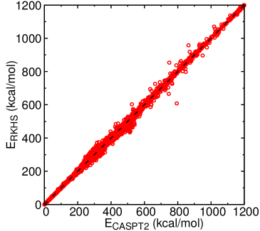
Figure 5: Correlation between the RKHS and CASPT2 energies for 16063 training data for N₄ system. The black dashed line shows ideal correlation between reference data and representation.

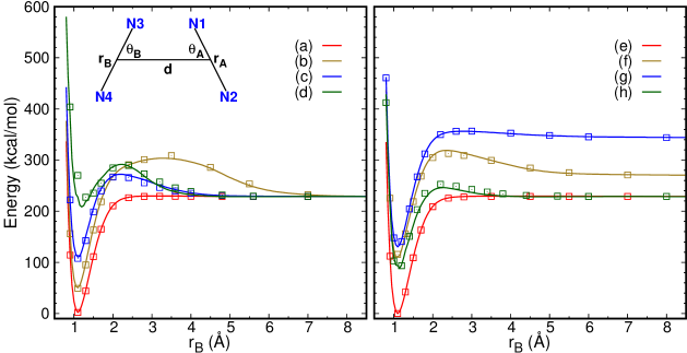
Figure 6: Comparison between the test ab initio data (symbols) and RKHS interpolated energies (solid lines) for the dissociation curves N3-N4 (along $r_{B}$) for N₂+N₂ system with N1-N2 fixed at $r_{A}$. The angle between $r_{A}$ and $r_{B}$ is defined as $\phi$. (a) $r_{A}$ = 1.098 Å, $d$ = 3.0 Å, $\theta_{A}$ = $\theta_{B}$ = 90^∘, $\phi$ = 0^∘ (b) $r_{A}$ = 1.098 Å, $d$ = 2.4 Å, $\theta_{A}$ = $\theta_{B}$ = 60^∘, $\phi$ = 0^∘ (c) $r_{A}$ = 1.098 Å, $d$ = 1.8 Å, $\theta_{A}$ = $\theta_{B}$ = 90^∘, $\phi$ = 90^∘ (d) $r_{A}$ = 1.098 Å, $d$ = 2.0 Å, $\theta_{A}$ = 0^∘, $\theta_{B}$ = 90^∘, $\phi$ = 0^∘ (e) $r_{A}$ = 1.098 Å, $d$ = 4.0 Å, $\theta_{A}$ = 120^∘, $\theta_{B}$ = 60^∘, $\phi$ = 0^∘ (f) $r_{A}$ = 1.298 Å, $d$ = 2.6 Å, $\theta_{A}$ = 0^∘, $\theta_{B}$ = 60^∘, $\phi$ = 0^∘ (g) $r_{A}$ = 0.898 Å, $d$ = 3.0 Å, $\theta_{A}$ = 0^∘, $\theta_{B}$ = 60^∘, $\phi$ = 0^∘ (h) $r_{A}$ = 1.098 Å, $d$ = 2.4 Å, $\theta_{A}$ = 0^∘, $\theta_{B}$ = 90^∘, $\phi$ = 0^∘.

Although techniques such as RKHS or permutationally invariant polynomials can provide accurate representations, their extensions to higher dimensions remains a challenge. Recently, the use of PIPs was demonstrated for the PES of N-methyl acetamide which is an important step in this direction.¹⁵⁵ Additionally, the (s)GDML approach^{156, 157} has been used to construct PESs for several small organic molecules, such as ethanol, malondialdehyde and aspirin.¹⁵⁸ Another challenge is to reduce the number of points required to define such a PES. Efforts in this direction have recently shown that with as few as 300 reference points the PES for scattering calculations in OH+H₂ can be described from a fit based on Gaussian processes together with Bayesian optimization.¹⁵⁹ Nevertheless, such high-accuracy representations of PESs for extended systems will remain a challenge for both, the number of high-quality reference calculations required and the type of inter- (and extra-)polation used to represent them.

Another important aspect of accurate studies of the energetics and dynamics of molecular systems concerns the observation, that “chemistry” is often local. As an example, the details of a chemical bond - its equilibrium separation and its strength - can depend sensitively on the local environment which may play an important role in applications such as infrared spectroscopy. As an example, singly methylated malonaldehyde is considered. Depending on the position of the proton, see Figure 7 the nature of the CO bond changes. Overall, there are chemically 4 different CO bonds, two single bonds (I)A and (I)B, and two double bonds (II)A and (II)B. In the language of an empirical force field, the equilibrium bond lengths and the force constants change between these two structures in a dynamical fashion, depending on the position of the transferring hydrogen atom. Capturing such effects within an empirical force field is possible, but laborious, as was recently done for the oxalate anion.¹⁶⁰

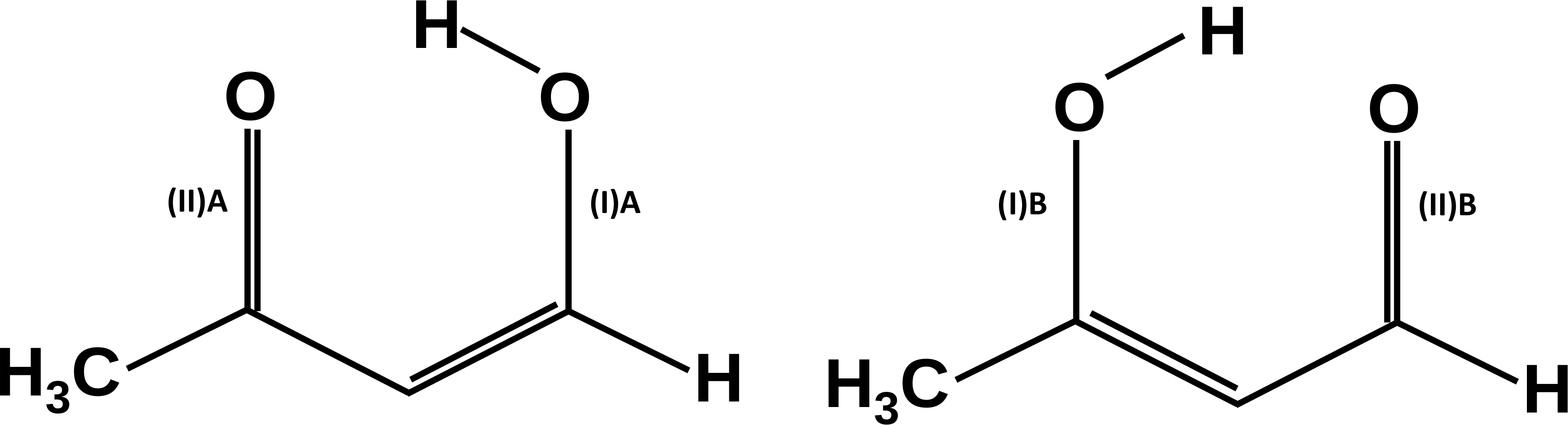
Figure 7: The structure and local bonding motifs in singly methylated malonaldehyde. Depending on the position of the transferring hydrogen atom different single ((I)A and (I)B) and double ((II)A and (II)B) bonds arise. The distribution of the electrons will modify the stretching frequencies and therefore the force constants and equilibrium bond lengths. From optimizations at the MP2/6-31G(d,p) level the equilibrium separations of the single bonds (I)A and (I)B are 1.3224 Å and 1.3255 Å which compare with 1.2475 Å and 1.2462 Å for the double bonds (II)A and (II)B, respectively.

Capturing such effects within a NN-trained global PES using PhysNet is more convenient. As an example, the situation in singly-methylated malonaldehyde (acetoacetaldehyde, AAA) is considered, see Figure 7. There are two CO motifs each of which can carry the transferring hydrogen atom at the oxygen atom. Depending on whether the hydrogen atom is on the OC-CH₃ or OC-C side the chemical nature of the CO bond changes. This also influences the frequencies of the CO stretch vibrations. Figure 8 reports the infrared spectrum from normal modes from MP2/6-311G(d,p) calculations and from an NN trained on energies at the same level of theory. As is shown, the normal modes from the electronic structure calculations from the MP2/6-311G(d,p) for the two isomers (top and bottom panels) differ appreciably in the range of the amide-I stretches. Above 1600 cm^-1 the harmonic frequencies occur at 1644 and 1692 cm^-1 for isomer AAA1 and at 1658 and 1696 cm^-1 for isomer AAA2. The NN (middle two panels) is successful in capturing the higher frequency (at 1689 and 1695 cm^-1 for the two isomers, respectively) whereas for the lower frequency the two modes occur at 1635 and 1634 cm^-1. Additional modes involving CO stretch vibrations occur between 1400 and 1500 cm^-1. Figure 8 shows clear differences for the patterns for AAA1 and AAA2 which are correctly captured by the NN.

In a conventional force field all these frequencies would be nearly overlapping as the force field parameters for a CO bond does usually not depend on whether a hydrogen is bonded to it or not. In order to capture such an effect, the force field parameters for the CO bond would need to depend on the bonding pattern of the molecule along the dynamics trajectory. Encoding such detail into a conventional force field is difficult and NN-trained PESs offer a natural way to do so.

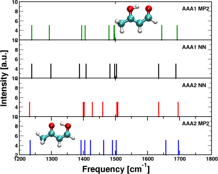
Figure 8: The infrared spectrum of methylated malonaldehyde in the region of the CO stretch region. The bands at higher frequency (above 1600 cm^-1 are due to C=O bonds whereas those between 1400 and 1500 cm^-1 involve a partial double bond for the CO stretch. The top and bottom panels are for normal modes from MP2/6-31G(d,p) calculations and the two middle panels from normal modes on the trained NN using PhysNet.

Another benefit yet to be explored that NN-trained PESs such as PhysNet offer is the possibility to have fluctuating point charges for a molecule without the need to explicitly parametrize the dependence on the geometry. Modeling such effects within an empirical force field is challenging.¹⁶¹

A final challenge for high-dimensional PESs is including the chemical environment, such as the effect of a solvent. Immersing a chemically reacting system into an environment leads to pronounced changes. As an example, double proton transfer in formic acid dimer in the gas phase and in solution is considered. The parametrization used here was adapted to yield the correct infrared spectrum in the gas phase.¹⁶² Recent high-resolution work has confirmed that the barrier of 7.3 kcal/mol for the gas-phase PES is compatible with the tunneling splitting observed in microwave studies.¹⁶³ Such a barrier height makes spontaneous transitions rare. Hence, umbrella sampling simulations were combined with the molecular mechanics with proton transfer (MMPT) force field to determine the free energy barrier for DPT in the gas phase and in solution. As a comparison, the simulations were also carried out by using the Density-Functional Tight-Binding (DFTB)^{164, 165} method for the FAD. In both cases the solvent was water represented as the TIP3P model.¹⁶⁶

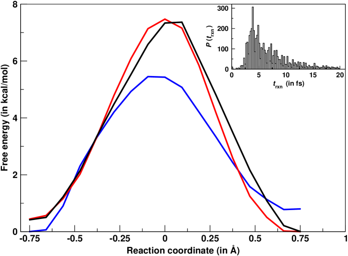
Figure 9: Free energy as a function of reaction coordinate for proton transfer in gaseous and water-solvated FAD. The blue and red curves show the free energy for FAD in the gas and solution phase respectively using the MMPT force field. The energy profile in black is obtained for FAD in solution through DFTB treatment. In all cases, for the umbrella sampling procedure, 17 umbrella windows are located at 0.1 Å intervals and trajectories are propagated for 50 ps. The probability distribution from different umbrellas are recombined using the weighted histogram analysis method (WHAM).¹⁶⁷

The free energy barrier in the gas phase is $\Delta G=5.4$ kcal/mol which increases to 7.5 kcal/mol in water, see Fig. 9. With DFTB3 the barrier height in solution is similar (7.3 kcal/mol) to that with the MMPT parametrization. In all cases, FAD undergoes a concerted double proton transfer to interconvert between two equivalent forms resulting in a symmetric potential. The nature of the transition state was verified by running 5000 structures from the umbrella sampling simulations at the TS, starting with zero velocity, and propagating them for 1 ps in an $NVE$ ensemble. The fraction of reactants and products obtained are 0.54 and 0.46, indicating that the configurations sampled in the umbrella sampling simulations indeed correspond to a transition state and lie midway between reactants and products and are equally likely to relax into either stable state.

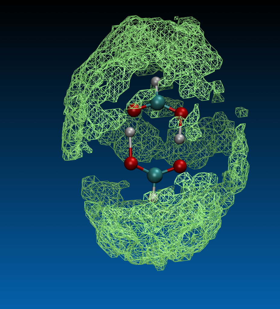
Figure 10: Solvent distribution around FAD for the transition state ensemble from 5000 transition states sampled from umbrella sampling simulations.

From these simulations it is also possible to determine the time to product or reactant which is reported in the the inset of Figure 9. The most probable time is $\sim 5$ fs with a wide distribution extending out to to 20 fs. This is typical for a waiting time distribution and indicates that multiple degrees of freedom are involved.

The methods discussed in the present work have all their advantages and shortcomings. Depending on the application at hand the methods provide different efficiencies and accuracies and are more or less straightforward to apply. In the following, the three approaches discussed here are compared by looking at them from different perspectives.

• For small gas phase systems such as tri- and tetraatomics, RKHSs, PIPs and NN-based force fields are powerful methods for accurate investigations of their reactive dynamics. Empirical force fields are clearly not intended and suitable for this.

• For medium-sized molecules (up to $\sim 10$ atoms) in the gas phase, reactive MD methods, such as EVB¹⁶⁸ (not explicitly discussed here or multi state reactive MD), NNs, or suitably parametrized force fields (polarizable or non-polarizable) including multipoles are viable representations. PIPs or RKHSs will eventually become cumbersome to parametrize and computationally expensive to evaluate.

• Systems with $\sim 10$ atoms in solution can be described by refined FFs and reactive MD simulations. NNs, such as Physnet, would be a very attractive possibility, as they include fluctuating charges by construction. Also, capturing changes in the bond character depending on the chemical environment (see discussion of methylated MA above) is readily possible. However, an open technical question is how to include the effect of the environment in training the NN.

• Finally, for macromolecules in solution, such as proteins, either refined reactive FFs or a combination of RKHS and a FF has shown to provide meaningful ways to extend quantitative, reactive simjlations to condensed phase systems. Extending such approaches, akin to mixed QM/MM simulations but treating the reactive part with a NN, may provide even better accuracy.

Multidimensional PESs are a powerful way to run high-quality atomistic simulations for gas- and condensed phase systems. Recent progress concerns the accurate, routine representation of PESs based on RKHSs or PIPs. As an exciting alternative, NN-based PESs have also become available. Despite this progress, extension of these techniques to simulations in solution and multiple dimensions remain a challenge. Attractive future possibilities are simulations which capture the changes in local chemistry or in the atomic charges without the need to explicitly parametrize them as a function of geometry. This is possible with approaches as those used in PhysNet.

References

- El Hage et al. 2017 El Hage, K.; Brickel, S.; Hermelin, S.; Gaulier, G.; Schmidt, C.; Bonacina, L.; van Keulen, S. C.; Bhattacharyya, S.; Chergui, M.; Hamm, P.; Rothlisberger, U.; Wolf, J.-P.; Meuwly, M. Implications of short time scale dynamics on long time processes. Struct. Dyn. 2017, 4
- Minitti et al. 2015 Minitti, M. P. et al. Imaging Molecular Motion: Femtosecond X-Ray Scattering of an Electrocyclic Chemical Reaction. Phys. Rev. Lett. 2015, 114
- Cui and Karplus 2008 Cui, Q.; Karplus, M. Allostery and cooperativity revisited. Prot. Sci. 2008, 17, 1295–1307
- Nussinov and Tsai 2015 Nussinov, R.; Tsai, C.-J. Allostery without a conformational change? Revisiting the paradigm. Curr. Opin. Struc. Biol. 2015, 30, 17–24
- Cooper and Dryden 1984 Cooper, A.; Dryden, D. T. F. Allostery without conformational change. Eur. Biophys. J. 1984, 11, 103–109
- Alon 2007 Alon, U. An introduction to systems biology: Design principles and biological c ircuits; Chapman & Hall/CRC: London, 2007
- Cui 2016 Cui, Q. Perspective: Quantum mechanical methods in biochemistry and biophysics. J. Chem. Phys. 2016, 145
- Senn and Thiel 2009 Senn, H. M.; Thiel, W. QM/MM Methods for Biomolecular Systems. Angew. Chem. Intern. Ed. 2009, 48, 1198–1229
- Roston et al. 2016 Roston, D.; Demapan, D.; Cui, Q. Leaving Group Ability Observably Affects Transition State Structure in a Single Enzyme Active Site. J. Am. Chem. Soc. 2016, 138, 7386–7394
- Kulik et al. 2016 Kulik, H. J.; Zhang, J.; Klinman, J. P.; Martinez, T. J. How Large Should the QM Region Be in QM/MM Calculations? The Case of Catechol O-Methyltransferase. J. Phys. Chem. B 2016, 120, 11381–11394
- Rasmussen et al. 2007 Rasmussen, T. D.; Ren, P.; Ponder, J. W.; Jensen, F. Force Field Modeling of Conformational Energies: Importance of Multipole Moments and Intramolecular Polarization. Int. J. Quant. Chem. 2007, 107, 1390–1395
- Kramer et al. 2013 Kramer, C.; Gedeck, P.; Meuwly, M. Multipole-Based Force Fields from ab Initio Interaction Energies and the Need for Jointly Refitting All Intermolecular Parameters. J. Chem. Theo. Comp. 2013, 9, 1499–1511
- Bereau et al. 2013 Bereau, T.; Kramer, C.; Meuwly, M. Leveraging Symmetries of Static Atomic Multipole Electrostatics in Molecular Dynamics Simulations. J. Chem. Theo. Comp. 2013, 9, 5450–5459
- Shi et al. 2013 Shi, Y.; Xia, Z.; Zhang, J.; Best, R.; Wu, C.; Ponder, J. W.; Ren, P. Polarizable Atomic Multipole-Based AMOEBA Force Field for Proteins. J. Chem. Theo. Comp. 2013, 9, 4046–4063
- Lopes et al. 2013 Lopes, P. E. M.; Huang, J.; Shim, J.; Luo, Y.; Li, H.; Roux, B.; MacKerell, A. D., Jr. Polarizable Force Field for Peptides and Proteins Based on the Classical Drude Oscillator. J. Chem. Theo. Comp. 2013, 9, 5430–5449
- Braams and Bowman 2009 Braams, B. J.; Bowman, J. M. Permutationally invariant potential energy surfaces in high dimensionality. Int. Rev. Phys. Chem. 2009, 28, 577–606
- Xie and Bowman 2010 Xie, Z.; Bowman, J. M. Permutationally Invariant Polynomial Basis for Molecular Energy Surface Fitting via Monomial Symmetrization. J. Chem. Theo. Comp. 2010, 6, 26–34
- Jin et al. 2006 Jin, Z.; Braams, B.; Bowman, J. An ab initio based global potential energy surface describing CH5+ -¿ CH3++H-2. J. Phys. Chem. A 2006, 110, 1569–1574
- Huang et al. 2006 Huang, X.; Johnson, L.; Bowman, J.; McCoy, A. Deuteration effects on the structure and infrared spectrum of CH5+. J. Am. Chem. Soc. 2006, 128, 3478–3479
- Huang et al. 2008 Huang, X.; Braams, B. J.; Bowman, J. M.; Kelly, R. E. A.; Tennyson, J.; Groenenboom, G. C.; van der Avoird, A. New ab initio potential energy surface and the vibration-rotation-tunneling levels of (H2O)(2) and (D2O)(2). J. Chem. Phys. 2008, 128
- Wang et al. 2011 Wang, Y.; Huang, X.; Shepler, B. C.; Braams, B. J.; Bowman, J. M. Flexible, ab initio potential, and dipole moment surfaces for water. I. Tests and applications for clusters up to the 22-mer. J. Chem. Phys. 2011, 134
- Shepler et al. 2007 Shepler, B. C.; Braams, B. J.; Bowman, J. M. Quasiclassical trajectory calculations of acetaldehyde dissociation on a global potential energy surface indicate significant non-transition state dynamics. J. Phys. Chem. A 2007, 111, 8282–8285
- Varandas 1988 Varandas, A. Intermolecular and Intramolecular Potentials - Topographical Aspects, Calculation, and functional Representation via a Double Many-Body Expansion Method. Adv. Chem. Phys. 1988, 74, 255–338
- Goncalves et al. 2018 Goncalves, C. E. M.; Galvao, B. R. L.; Mota, V. C.; Braga, J. P.; Varandas, A. J. C. Accurate Explicit-Correlation-MRCI-Based DMBE Potential-Energy Surface for Ground-State CNO. J. Phys. Chem. A 2018, 122, 4198–4207
- Koner et al. 2018 Koner, D.; Bemish, R. J.; Meuwly, M. The C(3P) + NO(X ) O(3P) + CN(X ), N(2D)/N(4S) + CO(X )) reaction: Rates, branching ratios, and final states from 15 K to 20 000 K. J. Chem. Phys. 2018, 149
- Collins 2002 Collins, M. A. Molecular Potential-Energy Surfaces for Chemical Reaction Dynamics. Theor. Chem. Acc. 2002, 108, 313–324
- Dawes et al. 2009 Dawes, R.; Passalacqua, A.; Wagner, A. F.; Sewell, T. D.; Minkoff, M.; Thompson, D. L. Interpolating moving least-squares methods for fitting potential energy surfaces: Using classical trajectories to explore configuration space. J. Chem. Phys. 2009, 130
- Quintas-Sanchez and Dawes 2019 Quintas-Sanchez, E.; Dawes, R. AUTOSURF: A Freely Available Program To Construct Potential Energy Surfaces. J. Chem. Inf. Model. 2019, 59, 262–271
- Rupp et al. 2012 Rupp, M.; Tkatchenko, A.; Müller, K.-R.; Von Lilienfeld, O. A. Fast and Accurate Modeling of Molecular Atomization Energies with Machine Learning. Phys. Rev. Lett. 2012, 108, 058301
- Montavon et al. 2013 Montavon, G.; Rupp, M.; Gobre, V.; Vazquez-Mayagoitia, A.; Hansen, K.; Tkatchenko, A.; Müller, K.-R.; Von Lilienfeld, O. A. Machine Learning of Molecular Electronic Properties in Chemical Compound Space. New J. Phys. 2013, 15, 095003
- Hansen et al. 2013 Hansen, K.; Montavon, G.; Biegler, F.; Fazli, S.; Rupp, M.; Scheffler, M.; Von Lilienfeld, O. A.; Tkatchenko, A.; Müller, K.-R. Assessment and Validation of Machine Learning Methods for Predicting Molecular Atomization Energies. J. Chem. Theory Comput. 2013, 9, 3404–3419
- Hansen et al. 2015 Hansen, K.; Biegler, F.; Ramakrishnan, R.; Pronobis, W.; Von Lilienfeld, O. A.; Müller, K.-R.; Tkatchenko, A. Machine learning predictions of molecular properties: Accurate many-body potentials and nonlocality in chemical space. J. Phys. Chem. Lett 2015, 6, 2326–2331
- Samuel 2000 Samuel, A. L. Some studies in machine learning using the game of checkers. IBM J. Res. Dev. 2000, 44, 206–226
- Schölkopf et al. 1997 Schölkopf, B.; Smola, A.; Müller, K.-R. Kernel principal component analysis. International conference on artificial neural networks. 1997; pp 583–588
- Boser et al. 1992 Boser, B. E.; Guyon, I. M.; Vapnik, V. N. A training algorithm for optimal margin classifiers. Proceedings of the fifth annual workshop on Computational learning theory. 1992; pp 144–152
- Schölkopf et al. 1998 Schölkopf, B.; Smola, A.; Müller, K.-R. Nonlinear component analysis as a kernel eigenvalue problem. Neural Comput. 1998, 10, 1299–1319
- Theodoridis et al. 2008 others,, et al. Pattern Recognition; Elsevier, 2008
- Behler 2011 Behler, J. Atom-Centered Symmetry Functions for Constructing High-Dimensional Neural Network Potentials. J. Chem. Phys. 2011, 134, 074106
- Bartók et al. 2013 Bartók, A. P.; Kondor, R.; Csányi, G. On representing chemical environments. Phys. Rev. B 2013, 87, 184115
- Faber et al. 2018 Faber, F. A.; Christensen, A. S.; Huang, B.; von Lilienfeld, O. A. Alchemical and structural distribution based representation for universal quantum machine learning. J. Chem. Phys. 2018, 148, 241717
- Christensen et al. 2019 Christensen, A. S.; Bratholm, L. A.; Faber, F. A.; Glowacki, D. R.; von Lilienfeld, O. A. FCHL revisited: faster and more accurate quantum machine learning. arXiv preprint arXiv:1909.01946 2019,
- Schütt et al. 2014 Schütt, K.; Glawe, H.; Brockherde, F.; Sanna, A.; Müller, K.; Gross, E. How to represent crystal structures for machine learning: Towards fast prediction of electronic properties. Phys. Rev. B 2014, 89, 205118
- Faber et al. 2015 Faber, F.; Lindmaa, A.; von Lilienfeld, O. A.; Armiento, R. Crystal structure representations for machine learning models of formation energies. Int. J. Quantum Chem. 2015, 115, 1094–1101
- Faber et al. 2016 Faber, F. A.; Lindmaa, A.; Von Lilienfeld, O. A.; Armiento, R. Machine Learning Energies of 2 Million Elpasolite (ABC2D6) Crystals. Phys. Rev. Lett. 2016, 117, 135502
- Schölkopf et al. 2001 Schölkopf, B.; Herbrich, R.; Smola, A. J. A Generalized Representer Theorem. International Conference on Computational Learning Theory. 2001; pp 416–426
- Berlinet and Thomas-Agnan 2011 Berlinet, A.; Thomas-Agnan, C. Reproducing Kernel Hilbert Spaces in Probability and Statistics; Springer Science & Business Media Dordrecht, 2011
- Hollebeek et al. 1999 Hollebeek, T.; Ho, T.-S.; Rabitz, H. Constructing multidimensional molecular potential energy surfaces from ab initio data. Ann. Rev. Phys. Chem. 1999, 50, 537–570
- Soldan and Hutson 2000 Soldan, P.; Hutson, J. On the long-range and short-range behavior of potentials from reproducing kernel Hilbert space interpolation. J. Chem. Phys. 2000, 112, 4415–4416
- Müller et al. 2001 Müller, K.-R.; Mika, S.; Rätsch, G.; Tsuda, K.; Schölkopf, B. An introduction to kernel-based learning algorithms. IEEE Trans. Neural Netw. 2001, 12
- Hofmann et al. 2008 Hofmann, T.; Schölkopf, B.; Smola, A. J. Kernel methods in machine learning. Ann. Stat. 2008, 1171–1220
- Golub and Van Loan 2012 Golub, G. H.; Van Loan, C. F. Matrix Computations; JHU Press Baltimore, 2012; Vol. 3
- Tikhonov et al. 1977 Tikhonov, A. N.; Arsenin, V. I.; John, F. Solutions of Ill-Posed Problems; Winston Washington, DC, 1977; Vol. 14
- Rupp 2015 Rupp, M. Machine Learning for Quantum Mechanics in a Nutshell. Int. J. Quantum Chem. 2015, 115, 1058–1073
- Rasmussen and Williams 2005 Rasmussen, C.; Williams, C. GAUSSIAN PROCESSES FOR MACHINE LEARNING; Adaptive Computation and Machine Learning; 2005; pp 1–247
- McCulloch and Pitts 1943 McCulloch, W. S.; Pitts, W. A Logical Calculus of the Ideas Immanent in Nervous Activity. Bull. Math. Biophys. 1943, 5, 115–133
- Kohonen 1988 Kohonen, T. An Introduction to Neural Computing. Neural Netw. 1988, 1, 3–16
- Abdi 1994 Abdi, H. A Neural Network Primer. J. Biol. Syst. 1994, 2, 247–281
- Bishop 1995 Bishop, C. M. Neural Networks for Pattern Recognition; Oxford university press, 1995
- Clark 1999 Clark, J. W. Scientific Applications of Neural Nets; Springer, 1999; pp 1–96
- Ripley 2007 Ripley, B. D. Pattern Recognition and Neural Networks; Cambridge university press, 2007
- Haykin 2009 Haykin, S. S. Neural Networks and Learning Machines; Pearson Upper Saddle River, NJ, USA:, 2009; Vol. 3
- Cybenko 1989 Cybenko, G. Approximation by superposition of sigmoidal functions. Math. Control Signals Syst. 1989, 2, 303–314
- Hornik 1991 Hornik, K. Approximation Capabilities of Multilayer Feedforward Networks. Neural Netw. 1991, 4, 251–257
- Eldan and Shamir 2016 Eldan, R.; Shamir, O. The Power of Depth for Feedforward Neural Networks. Conference on Learning Theory. 2016; pp 907–940
- Blank et al. 1995 Blank, T. B.; Brown, S. D.; Calhoun, A. W.; Doren, D. J. Neural network models of potential energy surfaces. J. Chem. Phys. 1995, 103, 4129–4137
- Brown et al. 1996 Brown, D. F.; Gibbs, M. N.; Clary, D. C. Combining ab initio computations, neural networks, and diffusion Monte Carlo: An efficient method to treat weakly bound molecules. J. Chem. Phys. 1996, 105, 7597–7604
- Tafeit et al. 1996 Tafeit, E.; Estelberger, W.; Horejsi, R.; Moeller, R.; Oettl, K.; Vrecko, K.; Reibnegger, G. Neural networks as a tool for compact representation of ab initio molecular potential energy surfaces. J. Mol. Graph. 1996, 14, 12–18
- No et al. 1997 No, K. T.; Chang, B. H.; Kim, S. Y.; Jhon, M. S.; Scheraga, H. A. Description of the potential energy surface of the water dimer with an artificial neural network. Chem. Phys. Lett. 1997, 271, 152–156
- Prudente and Neto 1998 Prudente, F. V.; Neto, J. S. The fitting of potential energy surfaces using neural networks. Application to the study of the photodissociation processes. Chem. Phys. Lett. 1998, 287, 585–589
- Manzhos and Carrington Jr 2006 Manzhos, S.; Carrington Jr, T. A Random-Sampling High Dimensional Model Representation Neural Network for Building Potential Energy Surfaces. J. Chem. Phys. 2006, 125, 084109
- Manzhos and Carrington Jr 2007 Manzhos, S.; Carrington Jr, T. Using Redundant Coordinates to Represent Potential Energy Surfaces with Lower-Dimensional Functions. J. Chem. Phys. 2007, 127, 014103
- Malshe et al. 2009 Malshe, M.; Narulkar, R.; Raff, L.; Hagan, M.; Bukkapatnam, S.; Agrawal, P.; Komanduri, R. Development of Generalized Potential-Energy Surfaces using Many-Body Expansions, Neural Networks, and Moiety Energy Approximations. J. Chem. Phys. 2009, 130, 184102
- Behler and Parrinello 2007 Behler, J.; Parrinello, M. Generalized Neural-Network Representation of High-Dimensional Potential-Energy Surfaces. Phys. Rev. Lett. 2007, 98, 146401
- Khorshidi and Peterson 2016 Khorshidi, A.; Peterson, A. A. Amp: a modular approach to machine learning in atomistic simulations. Comput. Phys. Commun. 2016, 207, 310–324
- Artrith et al. 2017 Artrith, N.; Urban, A.; Ceder, G. Efficient and accurate machine-learning interpolation of atomic energies in compositions with many species. Phys. Rev. B 2017, 96, 014112
- Unke and Meuwly 2018 Unke, O. T.; Meuwly, M. A reactive, scalable, and transferable model for molecular energies from a neural network approach based on local information. J. Chem. Phys. 2018, 148, 241708
- Smith et al. 2017 Smith, J. S.; Isayev, O.; Roitberg, A. E. ANI-1: An extensible neural network potential with DFT accuracy at force field computational cost. Chem. Sci. 2017, 8, 3192–3203
- Yao et al. 2018 Yao, K.; Herr, J. E.; Toth, D. W.; Mckintyre, R.; Parkhill, J. The TensorMol-0.1 model chemistry: A neural network augmented with long-range physics. Chem. Sci. 2018, 9, 2261–2269
- Gilmer et al. 2017 Gilmer, J.; Schoenholz, S. S.; Riley, P. F.; Vinyals, O.; Dahl, G. E. Neural Message Passing for Quantum Chemistry. International Conference on Machine Learning. 2017; pp 1263–1272
- Schütt et al. 2017 Schütt, K. T.; Arbabzadah, F.; Chmiela, S.; Müller, K. R.; Tkatchenko, A. Quantum-Chemical Insights from Deep Tensor Neural Networks. Nat. Commun. 2017, 8, 13890
- Schuett et al. 2017 Schuett, K. T.; Kindermans, P.-J.; Sauceda, H. E.; Chmiela, S.; Tkatchenko, A.; Mueller, K.-R. SchNet: A continuous-filter convolutional neural network for modeling quantum interactions. ADVANCES IN NEURAL INFORMATION PROCESSING SYSTEMS 30 (NIPS 2017). 2017; 31st Annual Conference on Neural Information Processing Systems (NIPS), Long Beach, CA, 2017
- Lubbers et al. 2018 Lubbers, N.; Smith, J. S.; Barros, K. Hierarchical modeling of molecular energies using a deep neural network. J. Chem. Phys. 2018, 148, 241715
- Unke and Meuwly 2019 Unke, O. T.; Meuwly, M. PhysNet: a neural network for predicting energies, forces, dipole moments and partial charges. J. Chem. Theo. Comp. 2019,
- Schütt et al. 2018 Schütt, K. T.; Gastegger, M.; Tkatchenko, A.; Müller, K.-R. Quantum-chemical insights from interpretable atomistic neural networks. arXiv preprint arXiv:1806.10349 2018,
- Armenise and Esposito 2015 Armenise, I.; Esposito, F. . Chem. Phys. 2015, 446, 30–46
- Dean et al. 1991 Dean, A. J.; Hanson, R. K.; Bowman, C. T. . J. Phys. Chem. 1991, 95, 3180
- Bergeat et al. 1999 Bergeat, A.; Calvo, T.; Dorthe, G.; Loison, J. C. . Chem. Phys. Lett. 1999, 308, 7
- Braun et al. 1969 Braun, W.; Bass, A. M.; Davis, D. D.; Simmons, J. D. Proc. Roy. Soc. A. 1969, 312, 417–434
- Landau 1932 Landau, L. D. . Phys. Z 1932, 2, 46
- Zener 1932 Zener, C. . Proc. R. Soc. London A 1932, 137, 696
- Belyaev and Lebedev 2011 Belyaev, A. K.; Lebedev, O. V. . Phys. Rev. A 2011, 84, 014701
- Belyaev et al. 2014 Belyaev, A. K.; Lasser, C.; Trigila, G. . J. Chem. Phys. 2014, 140, 224108
- Bird 1994 Bird, G. A. Molecular Gas Dynamics and the Direct Simulation of Gas Flows; Clarendon Press, 1994
- Rivero et al. 2019 Rivero, U.; Unke, T., Oliver; Meuwly, M.; Willitsch, S. A computational study of the Diels-Alder reactions between 2,3-dibromo-1,3-butadiene and maleic anhydride. J. Chem. Phys. 2019, qqq, qqq
- Chang et al. 2013 Chang, Y.-P.; Dlugolecki, K.; Küpper, J.; Rösch, D.; Wild, D.; Willitsch, S. Science 2013, 342, 98
- Willitsch 2017 Willitsch, S. Adv. Chem. Phys. 2017, 162, 307
- de Souza et al. 2016 de Souza, M. A. F.; Ventura, E.; do Monte, S. A.; Riveros, J. M.; Longo, R. L. J. Comput. Chem. 2016, 37, 701
- Black et al. 2012 Black, K.; Liu, P.; Xu, L.; Doubleday, C.; Houk, K. N. PNAS 2012, 109, 12860
- Tan et al. 2018 Tan, J. S. J.; Hirvonen, V.; Paton, R. S. Org. Lett. 2018, 20, 2821
- Wang et al. 2009 Wang, Z.; Hirschi, J. S.; Singleton, D. A. Angew. Chem. Int. Ed. 2009, 48, 9156
- Liu et al. 2016 Liu, F.; Yang, Z.; Mei, Y.; Houk, K. N. J. Phys. Chem. B 2016, 120, 6250
- Soto-Delgado et al. 2016 Soto-Delgado, J.; Tapia, R. A.; Torras, J. J. Chem. Theory Comput. 2016, 12, 4735
- Unke et al. 2019 Unke, O. T.; Brickel, S.; Meuwly, M. Sampling reactive regions in phase space by following the minimum dynamic path. J. Chem. Phys. 2019, 150, 074107
- Brickel et al. 2019 Brickel, S.; Das, A. K.; Unke, O. T.; Turan, H. T.; Meuwly, M. Reactive molecular dynamics for the [Cl–CH3–Br]- reaction in the gas phase and in solution: a comparative study using empirical and neural network force fields. Electronic Structure 2019, 1, 024002
- Schmid et al. 2018 Schmid, M.; Das, A. K.; Landis, C. R.; Meuwly, M. Multi-State VALBOND for Atomistic Simulations of Hypervalent Molecules, Metal Complexes and Reactions. J. Chem. Theo. Comp. 2018, in print
- Soloviov et al. 2016 Soloviov, M.; Das, A. K.; Meuwly, M. Structural Interpretation of Metastable States in Myoglobin-NO. Angew. Chem. Intern. Ed. 2016, 55, 10126–10130
- Unke and Meuwly 2017 Unke, O. T.; Meuwly, M. Toolkit for the Construction of Reproducing Kernel-Based Representations of Data: Application to Multidimensional Potential Energy Surfaces. J. Chem. Inf. Model. 2017, 57, 1923–1931
- Cornelius et al. 1983 Cornelius, P.; Hochstrasser, R.; Steele, A. Ultrafast relaxatio nin picosecond photolysis of nitrosylhemoglobin. J. Mol. Biol. 1983, 163, 119–128
- Petrich et al. 1991 Petrich, J. W.; Lambry, J. C.; Kuczera, K.; Karplus, M.; Poyart, C.; Martin, J. L. Ligand binding and protein relaxation in heme proteins: a room temperature analysis of nitric oxide geminate recombination. Biochem. 1991, 30, 3975–3987
- Ionascu et al. 2005 Ionascu, D.; Gruia, F.; Ye, X.; Yu, A.; Rosca, F.; Demidov, C. B. A.; Olson, J. S.; Champion, P. M. Temperature-dependent studies of NO recombination to heme and heme proteins. J. Am. Chem. Soc. 2005, 127, 16921–16934
- Kruglik et al. 2010 Kruglik, S. G.; Yoo, B.-K.; Franzen, S.; Vos, M. H.; Martin, J.-L.; Negrerie, M. Picosecond primary structural transition of the heme is retarded after nitric oxide binding to heme proteins. Proc. Natl. Acad. Sci. 2010, 107, 13678–13683
- Kim et al. 2012 Kim, J.; Park, J.; Lee, T.; Lim, M. Dynamics of Geminate Rebinding of NO with Cytochrome c in Aqueous Solution Using Femtosecond Vibrational Spectroscopy. J. Phys. Chem. B 2012, 116, 13663–13671
- Yoo et al. 2012 Yoo, B.-K.; Kruglik, S. G.; Lamarre, I.; Martin, J.-L.; Negrerie, M. Absorption Band III Kinetics Probe the Picosecond Heme Iron Motion Triggered by Nitric Oxide Binding to Hemoglobin and Myoglobin. J. Phys. Chem. B 2012, 116, 4106–4114
- Silatani et al. 2015 Silatani, M.; Lima, F. A.; Penfold, T. J.; Rittmann, J.; Reinhard, M. E.; Rittmann-Frank, H. M.; Borca, C.; Grolimund, D.; Milne, C. J.; Chergui, M. NO binding kinetics in myoglobin investigated by picosecond Fe K-edge absorption spectroscopy. Proc. Natl. Acad. Sci. 2015, 112, 12922–12927
- Kim et al. 2004 Kim, S.; Jin, G.; Lim, M. Dynamics of Geminate Recombination of NO with Myoglobin in Aqueous Solution Probed by Femtosecond Mid-IR Spectroscopy. J. Phys. Chem. B 2004, 108, 20366–20375
- Meuwly et al. 2002 Meuwly, M.; Becker, O. M.; Stote, R.; Karplus, M. NO rebinding to myoglobin: A reactive molecular dynamics study. Biophys. Chem. 2002, 98, 183–207
- Ye et al. 2002 Ye, X.; Demidov, A.; Champion, P. Measurements of the photodissociation quantum yields of MbNO and MbO(2) and the vibrational relaxation of the six-coordinate heme species. J. Am. Chem. Soc. 2002, 124, 5914–5924
- Nutt and Meuwly 2006 Nutt, D. R.; Meuwly, M. Studying reactive processes with classical dynamics: Rebinding dynamics in MbNO. Biophys. J. 2006, 90, 1191–1201
- Danielsson and Meuwly 2008 Danielsson, J.; Meuwly, M. Atomistic simulation of adiabatic reactive processes based on multi-state potential energy surfaces. J. Chem. Theo. Comp. 2008, 4, 1083
- Merchant et al. 2003 Merchant, K. A.; Noid, W. G.; Thompson, D. E.; Akiyama, R.; Loring, R. F.; Fayer, M. D. Structural assignments and dynamics of the A substates of MbCO: spectrally resolved vibrational echo experiments and molecular dynamics simulations. J. Phys. Chem. B 2003, 107, 4–7
- Claisen 1912 Claisen, L. Über Umlagerung von Phenol-allyläthern in C-Allyl-phenole. Chem. Ber. 1912, 45, 3157–3166
- Iwakura 2011 Iwakura, I. The Experimental Visualisation of Molecular Structural Changes During Both Photochemical and Thermal Reactions by Real-Time Vibrational Spectroscopy. Phys. Chem. Chem. Phys. 2011, 13, 5546–5555
- Coates et al. 1987 Coates, R. M.; Rogers, B. D.; Hobbs, S. J.; Curran, D. P.; Peck, D. R. Synthesis and Claisen Rearrangement of Alkoxyallyl Enol Ethers. Evidence for a Dipolar Transition State. J. Am. Chem. Soc. 1987, 35, 2601–2605
- Ziegler 1988 Ziegler, F. E. The Thermal, Aliphatic Claisen Rearrangement. Chem. Rev. 1988, 88, 1423–1452
- Severance and Jorgensen 1992 Severance, D. L.; Jorgensen, W. L. Effects of Hydration on the Claisen Rearrangement of Allyl Vinyl Ether from Computer Simulations. J. Am. Chem. Soc. 1992, 114, 10966–10968
- Guest et al. 1997 Guest, J. M.; Craw, J. S.; Vincent, M. A.; Hillier, I. H. The Effect of Water on the Claisen Rearrangement of Allyl Vinyl Ether: Theoretical Methods Including Explicit Solvent and Electron Correlation. Perkin Trans. 2 1997, 71–74
- Cramer and Truhlar 1992 Cramer, C. J.; Truhlar, D. G. ChemInform Abstract: What Causes Aqueous Acceleration of the Claisen Rearrangement? J Am Chem Soc 1992, 114, 8794–8799
- Kast et al. 1996 Kast, P.; Asif-Ullah, M.; Hilvert, D. Is Chorismate Mutase a Prototypic Entropy Trap? - Activation Parameters for the Bacillus Subtilis Enzyme. Tetrahedron Lett. 1996, 37, 2691–2694
- Ranaghan et al. 2003 Ranaghan, K. E.; Ridder, L.; Szefczyk, B.; Sokalski, W. A.; Hermann, J. C.; Mulholland, A. J. Insights Into Enzyme Catalysis from QM/MM Modelling: Transition State Stabilization in Chorismate Mutase. Mol. Phys. 2003, 101, 2695–2714
- Lever et al. 2014 Lever, G.; Cole, D. J.; Lonsdale, R.; Ranaghan, K. E.; Wales, D. J.; Mulholland, A. J.; Skylaris, C. K.; Payne, M. C. Large-Scale Density Functional Theory Transition State Searching in Enzymes. J. Phys. Chem. Lett. 2014, 5, 3614–3619
- Martí et al. 2010 Martí, S.; Andrés, J.; Moliner, V.; Silla, E.; Tuñón, I.; Bertrán, J. Theoretical QM/MM Studies of Enzymatic Pericyclic Reactions. Interdiscip. Sci. Comput. Life Sci. 2010, 2, 115–131
- Ferrer et al. 2011 Ferrer, S.; Martí, S.; Andrés, J.; Moliner, V.; Tuñón, I.; Bertrán, J. Molecular Mechanism of Chorismate Mutase Activity of Promiscuos MbtI. Theor. Chem. Acc. 2011, 128, 601–607
- Martí et al. 2001 Martí, S.; Andrés, J.; Moliner, V.; Silla, E.; Tuñón, I.; Bertrán, J.; Field, M. J. A Hybrid Potential Reaction Path and Free Energy Study of the Chorismate Mutase Reaction. J. Am. Chem. Soc. 2001, 123, 1709–1712
- Roca et al. 2009 Roca, M.; Vardi-Kilshtain, A.; Warshel, A. Toward Accurate Screening in Computer-Aided Enzyme Design. Biochemistry 2009, 48, 3046–3056
- Madurga and Vilaseca 2001 Madurga, S.; Vilaseca, E. SCRF Study of the Conformational Equilibrium of Chorismate in Water. Phys. Chem. Chem. Phys. 2001, 3, 3548–3554
- Davidson et al. 1997 Davidson, M. M.; Guest, J. M.; Craw, J. S.; Hillier, I. H.; Vincent, M. A. Conformational and Solvation Aspects of the Chorismate - Prephenate Rearrangement Studied by Ab Initio Electronic Structure and Simulation Methods. Perkin Trans. 2 1997, 1395–1400
- Wiest and Houk 1995 Wiest, O.; Houk, K. N. Stabilization of the Transition State of the Chorismate-Prephenate Rearrangement: An ab Initio Study of Enzyme and Antibody Catalysis. J. Am. Chem. Soc. 1995, 117, 11628–11639
- Hur and Bruice 2002 Hur, S.; Bruice, T. C. The Mechanism of Catalysis of the Chorismate to Prephenate Reaction by the Escherichia Coli Mutase Enzyme. Proc. Natl. Acad. Sci. U. S. A. 2002, 99, 1176–1181
- Vance and Rondan 1988 Vance, R.; Rondan, N. Transition Structures for the Claisen Rearrangement. J. Am. Chem. Soc. 1988, 110, 2314–2315
- Claeyssens et al. 2011 Claeyssens, F.; Ranaghan, K. E.; Lawan, N.; Macrae, S. J.; Manby, F. R.; Harvey, J. N.; Mulholland, A. J. Analysis of Chorismate Mutase Catalysis by QM/MM Modelling of Enzyme-Catalysed and Uncatalysed Reactions. Org. Biomol. Chem. 2011, 9, 1578–1590
- Ranaghan et al. 2004 Ranaghan, K. E.; Ridder, L.; Szefczyk, B.; Sokalski, W. A.; Hermann, J. C.; Mulholland, A. J. Transition State Stabilization and Substrate Strain in Enzyme Catalysis: Ab Initio QM/MM Modelling of the Chorismate Mutase Reaction. Org. Biomol. Chem. 2004, 2, 968–980
- Carlson and Jorgensen 1996 Carlson, H. A.; Jorgensen, W. L. Monte Carlo Investigations of Solvent Effects on the Chorismate to Prephenate Rearrangement. J. Am. Chem. Soc. 1996, 118, 8475–8484
- Andrews et al. 1973 Andrews, P. R.; Smith, G. D.; Young, I. G. Transition-State Stabilization and Enzymic Catalysis. Kinetic and Molecular Orbital Studies of the Rearrangement of Chorismate to Prephenate. Biochemistry 1973, 12, 3492–3498
- Wright et al. 2005 Wright, S.; DeClue, M.; Mandal, A.; Lee, L.; Wiest, O.; Cleland, W.; Hilvert, D. Isotope Effects on the Enzymatic and Nonenzymatic Reactions of Chorismate. J. Am. Chem. Soc. 2005, 127, 12957–12964
- Addadi et al. 1983 Addadi, L.; Jaffe, E. K.; Knowles, J. R. Secondary Tritium Isotope Effects as Probes of the Enzymic and Nonenzymic Conversion of Chorismate to Prephenate. Biochemistry 1983, 22, 4494–4501
- O’Ferrall 1970 O’Ferrall, R. A. M. Relationships between E2 and E1cB Mechanisms of -Elimination. J Chem Soc 1970, #, 274–277
- Jencks 1972 Jencks, W. P. General Acid-Base Catalysis of Complex Reactions in Water. Chem. Rev. 1972, 72, 705–718
- Ruddigkeit et al. 2012 Ruddigkeit, L.; Van Deursen, R.; Blum, L. C.; Reymond, J.-L. Enumeration of 166 billion organic small molecules in the chemical universe database GDB-17. Journal of chemical information and modeling 2012, 52, 2864–2875
- Faber et al. 2017 Faber, F. A.; Hutchison, L.; Huang, B.; Gilmer, J.; Schoenholz, S. S.; Dahl, G. E.; Vinyals, O.; Kearnes, S.; Riley, P. F.; Von Lilienfeld, O. A. Prediction errors of molecular machine learning models lower than hybrid DFT error. J. Chem. Theory Comput. 2017, 13, 5255–5264
- Ramakrishnan et al. 2014 Ramakrishnan, R.; Dral, P. O.; Rupp, M.; Von Lilienfeld, O. A. Quantum chemistry structures and properties of 134 kilo molecules. Sci. Data 2014, 1, 140022
- Schütt et al. 2019 Schütt, K.; Gastegger, M.; Tkatchenko, A.; Müller, K.-R.; Maurer, R. Unifying machine learning and quantum chemistry–a deep neural network for molecular wavefunctions. arXiv preprint arXiv:1906.10033 2019,
- Christensen et al. 2019 Christensen, A. S.; Faber, F. A.; von Lilienfeld, O. A. Operators in quantum machine learning: Response properties in chemical space. J. Chem. Phys. 2019, 150, 064105
- Paukku et al. 2013 Paukku, Y.; Yang, K. R.; Varga, Z.; Truhlar, D. G. Global ab initio ground-state potential energy surface of N4. J. Chem. Phys. 2013, 139, 044309
- Paukku et al. 2014 Paukku, Y.; Yang, K. R.; Varga, Z.; Truhlar, D. G. Erratum: Global ab initio ground-state potential energy surface of N4. J. Chem. Phys. 2014, 140, 019903
- Qu and Bowman 2019 Qu, C.; Bowman, J. M. A fragmented, permutationally invariant polynomial approach for potential energy surfaces of large molecules: Application to N-methyl acetamide. J. Chem. Phys. 2019, 150
- Chmiela et al. 2017 Chmiela, S.; Tkatchenko, A.; Sauceda, H. E.; Poltavsky, I.; Schütt, K. T.; Müller, K.-R. Machine learning of accurate energy-conserving molecular force fields. Sci. Adv. 2017, 3, e1603015
- Chmiela et al. 2019 Chmiela, S.; Sauceda, H. E.; Poltavsky, I.; Müller, K.-R.; Tkatchenko, A. sGDML: Constructing accurate and data efficient molecular force fields using machine learning. Comput. Phys. Commun. 2019,
- Sauceda et al. 2019 Sauceda, H. E.; Chmiela, S.; Poltavsky, I.; Müller, K.-R.; Tkatchenko, A. Construction of Machine Learned Force Fields with Quantum Chemical Accuracy: Applications and Chemical Insights. arXiv preprint arXiv:1909.08565 2019,
- Vargas-Hernandez et al. 2019 Vargas-Hernandez, R. A.; Guan, Y.; Zhang, D. H.; Krems, R., V Bayesian optimization for the inverse scattering problem in quantum reaction dynamics. New. J. Phys. 2019, 21
- Xu and Meuwly 2017 Xu, Z.-H.; Meuwly, M. Vibrational Spectroscopy and Proton Transfer Dynamics in Protonated Oxalate. J. Phys. Chem. A 2017, 121, 5389–5398
- Patel and Brooks 2004 Patel, S.; Brooks, C. CHARMM fluctuating charge force field for proteins: I parameterization and application to bulk organic liquid simulations. J. Comput. Chem. 2004, 25, 1–15
- Mackeprang et al. 2016 Mackeprang, K.; Xu, Z.-H.; Maroun, Z.; Meuwly, M.; Kjaergaard, H. G. Spectroscopy and dynamics of double proton transfer in formic acid dimer. Phys. Chem. Chem. Phys. 2016, 18, 24654–24662
- Li et al. 2019 Li, W.; Evangelisti, L.; Gou, Q.; Caminati, W.; Meyer, R. The Barrier to Proton Transfer in the Dimer of Formic Acid: A Pure Rotational Study. Angew. Chem. Intern. Ed. 2019, 58, 859–865
- Elstner et al. 1998 Elstner, M.; Porezag, D.; Jungnickel, G.; Elsner, J.; Haugk, M.; Frauenheim, T.; Suhai, S.; Seifert, G. Self-consistent-charge density-functional tight-binding method for simulations of complex materials proper ties. Phys. Rev. B 1998, 58, 7260–7268
- Gaus et al. 2014 Gaus, M.; Cui, Q.; Elstner, M. Density functional tight binding: application to organic and biological molecules. WIREs: Comput Mol Sci 2014, 4, 49–61
- Jorgensen et al. 1983 Jorgensen, W. L.; Chandrasekhar, J.; Madura, J. D.; Impey, R. W.; Klein, M. L. Comparison of simple potential functions for simulating liquid water. J. Chem. Phys. 1983, 79, 926–935
- Kumar et al. 1992 Kumar, S.; Rosenberg, J. M.; Bouzida, D.; Swendsen, R. H.; Kollman, P. A. The weighted histogram analysis method for free-energy calculations on biomolecules. I. The method. J. Comput. Chem. 1992, 13, 1011–1198
- Warshel and Weiss 1980 Warshel, A.; Weiss, R. An Empirical Valence Bond Approach for Comparing Reactions in Solutions and in Enzymes. J. Am. Chem. Soc. 1980, 102, 6218–6226