Orbital evolution of eccentric low-mass companions embedded in gaseous disks: testing the local approximation

Abstract

We study the tidal interaction between a low-mass companion (e.g., a protoplanet or a black hole) in orbit about a central mass, and the accretion disk within which it is submerged. We present results for a companion on a coplanar orbit with eccentricity $e$ between $0.1$ and $0.6$. For these eccentricities, dynamical friction arguments in its local approximation, that is, ignoring differential rotation and the curvature of the orbit, provide simple analytical expressions for the rates of energy and angular momentum exchange between the disk and the companion. We examine the range of validity of the dynamical friction approach by conducting a series of hydrodynamical simulations of a perturber with softening radius $R_{\rm soft}$ embedded in a two-dimensional disk. We find close agreement between predictions and the values in simulations provided that $R_{\rm soft}$ is chosen sufficiently small, below a threshold value $\stackrel{{\scriptstyle\sim}}{{\smash{R}\rule{0.0pt}{4.73611pt}}}_{\rm soft}$, which depends on the disk parameters and on $e$. We give $\stackrel{{\scriptstyle\sim}}{{\smash{R}\rule{0.0pt}{4.73611pt}}}_{\rm soft}$ for both razor-thin disks and disks with a finite scaleheight. For point-like perturbers, the local approximation is valid if the accretion radius is smaller than $\stackrel{{\scriptstyle\sim}}{{\smash{R}\rule{0.0pt}{4.73611pt}}}_{\rm soft}$. This condition imposes an upper value on the mass of the perturber.

1. Introduction

There are numerous studies about the tidal interaction between a disk in Keplerian rotation about a central mass and a low-mass companion. Determining the orbital evolution of the companion is crucial to understand a range of astrophysical scenarios. Embryos, protoplanetary cores and planets change its orbital parameters (semimajor axis $a$, eccentricity $e$ and inclination $i$) due to the mutual gravitational scatterings and due to the exchange of angular momentum and energy with the protoplanetary disk (e.g., Baruteau et al., 2014). Likewise, stars, stellar black holes and other compact objects experience orbital evolution within accretion disks around supermassive black holes in active galactic nuclei (e.g., Kocsis et al., 2011).

In this paper we are interested in the interaction between the disk and a companion in an eccentric and coplanar orbit with $e>0.1$. A substantial body of research has been directed to quantify the orbital evolution of eccentric perturbers through semianalytical models (e.g., Goldreich & Tremaine, 1980; Artymowicz, 1994; Papaloizou & Larwood, 2000; Goldreich & Sari, 2003; Tanaka & Ward, 2004; Muto et al., 2011). or using numerical simulations (e.g., Cresswell & Nelson, 2006; Cresswell et al., 2007; Marzari & Nelson, 2009; Bitsch & Kley, 2010, 2011; Bitsch et al., 2013; Fendyke & Nelson, 2014; Duffell & Chiang, 2015; Ragusa et al., 2018). For perturbers with such a small mass that they have a weak impact on the disk, these studies show that the response of the disk depends on the parameter $X\equiv e/h$, where $h$ is the aspect ratio of the disk (typically $h=0.04$). For small $X$, the perturber describes epicyclic motions of small amplitude, and it excites a trailing and a leading spiral wave, because of the Keplerian shear of the flow in its vicinity (e.g., Tanaka & Ward, 2004). As $X$ is raised, the mean velocity of the perturber relative to the local gas increases, and therefore the shear becomes less important. For instance, in the simulations of Cresswell et al. (2007) with $X=6$, a significant density enhancement appears in front of the perturber when it is at apocenter, whereas the enhancement lags behind it at pericenter.

The eccentricity distribution of exoplanets is broad, with a median value around $0.3$ (e.g., Marcy et al., 2005; Udry & Santos, 2007; Xie et al., 2016; Mills et al., 2019). Some extrasolar planets have eccentricities larger than $0.6$ (Wittenmyer et al., 2007; Tamuz et al., 2008). Motivated by these findings, we are concerned with the orbital evolution of a perturber having $X\gtrsim 3$. Theoretical predictions in this regime are scarce. Papaloizou & Larwood (2000) evaluate the torque acting on a low-mass perturber with $X\lesssim 5$, by including all Lindblad resonances required for convergence. The perturber was modeled using a softening radius between $0.4H$ and $H$, where $H$ is the scaleheight of the disk. For a disk with an initial surface density $\propto R^{-3/2}$ and a perturber with $X>1.1$, they find that the torque on the perturber is positive, and the eccentricity is damped in a timescale $\propto e^{3}$. They also note that the torque is rather sensitive to the softening radius. Consequently, the ambiguity in the definition of the softening radius to be used in real three-dimensional (3D) disks for eccentric orbits leads to an uncertainty in the magnitude of the torque. A 3D treatment of the wake excited within $H$ from the perturber is desirable because the wake at distances within $H$ from the perturber contributes to the torque. Another limitation of the resonance method is that it becomes impractical for arbitrary large $X$, say $X>5$, because the convergence is very slow.

For $X\gtrsim 3$, Muto et al. (2011) suggest that a dynamical friction approach may be a good approximation to estimate the migration timescale $\tau_{a}\equiv a/\dot{a}$ and the eccentricity damping timescale $\tau_{e}\equiv e/\dot{e}$ as the perturber moves supersonically relative to the local gas and the Keplerian shear is unimportant (see also Papaloizou, 2002; Rein, 2012). More specifically, they compute the force that the disk exerts on the perturber in the local approximation, that is, taking the local values of the disk surface density and sound speed at each point of the orbit, and evaluating the drag force as if the disk were homogeneous and the orbit rectilinear. Using this approximation, Muto et al. (2011) were able to predict $\tau_{a}$ and $\tau_{e}$ for a variety of disk models in a rather straightforward way.

Another virtue of the local approximation is that the formalism can be extended to include the vertical extent of the disk. In fact, Cantó et al. (2013) derive the drag force exerted on a perturber moving in rectilinear orbit in the midplane of a vertically-stratified slab. Thus, for those model parameters for which the local approximation is confirmed to be satisfactory in 2D models, we can apply the analytical expressions in Cantó et al. (2013) to evaluate $\tau_{a}$ and $\tau_{e}$, following the same approach as Muto et al. (2011), but now including properly the 3D structure of the wake, which is important for supersonic perturbers. Therefore it is essential to determine under which conditions the local approximation provides accurate results. To do so, we have carried out a set of 2D numerical simulations and performed a detailed comparison between numerical results and analytical predictions.

The paper is organized as follows. In Section 2, we describe the model and provide some relevant system quantities that characterize the tidal interaction between the disk and the satellite. Section 3 gives an overview of the dynamical friction approach in its local approximation. In Section 4, we compare the results of direct numerical simulations with the theoretical estimates based on the local approximation. Extensions to a 3D disk and to point-like perturbers are discussed in Section 5. Finally, our findings ae summarized in Section 6.

2. Model description

We consider a perturber (the companion) of mass $M_{p}$ in orbit around a central mass $M_{c}$ in the midplane of the accretion disk (i.e. coplanar orbit). We will asume that the ratio between masses, $q\equiv M_{p}/M_{c}$, is low enough that it cannot open a gap in the disk (i.e. type I migration in the terminology of planetary migration) and the perturbation induced in the disk is weak. The mass threshold $q_{\rm crit}$ to open a gap depends on the eccentricity; it increases as eccentricity increases (Hosseinbor et al., 2007). As a guide number, $q_{\rm crit}\simeq 10^{-3}$ for a perturber with $e=0.15$ embedded in a disk with a viscosity typical for protoplanetary disks. In this paper we will consider only $q<q_{\rm crit}$. In the limit of low mass, the timescales of migration and eccentricity damping will be much longer than the orbital period and, thus, we may use the osculating elements to describe the orbital evolution of the perturber.

The total force on the perturber is $\mbox{\boldmath$F$}{}_{t}=\mbox{\boldmath$F$}{}_{0}+\mbox{\boldmath$F$}{}_{1}$, where $\mbox{\boldmath$F$}{}_{0}$ is the gravitational force created by the central mass plus the unperturbed disk, and $\mbox{\boldmath$F$}{}_{1}$ is the backreaction force due to the density perturbations induced in the disk. In order to calculate the change rates of $a$ and $e$, we need the two components of $\mbox{\boldmath$F$}{}_{1}$ or, equivalently, the power ${\mathcal{P}}_{1}$ and the torque $T_{1}$ exerted on the perturber by the density wake excited in the disk. Along the paper, we will use the convention that $T_{1}$ is negative when the perturber loses angular momentum, and it is positive otherwise. The time derivatives of $a$ and $e$ can be computed using the Gauss equations as

$$\frac{da}{dt}=\frac{2{\mathcal{P}}_{1}}{a\omega^{2}M_{p}},$$ (1)

and

$$\frac{de}{dt}=\frac{\eta^{2}}{ea^{2}\omega^{2}M_{p}}\left(\mathcal{P}_{1}-\frac{\omega T_{1}}{\eta}\right).$$ (2)

where $\omega=\sqrt{GM_{c}/a^{3}}$ and $\eta=\sqrt{1-e^{2}}$. Note that the force component $\mbox{\boldmath$F$}{}_{0}$ cannot lead to a net radial migration or eccentricity damping.

As it will become clear later, it is useful to compute the velocity of the gas relative to the perturber. More specifically, we define the relative velocity as $\mbox{\boldmath$V$}{}_{\rm rel}=\mbox{\boldmath$v$}{}_{g}-\mbox{\boldmath$v$}{}_{p}$, where $\mbox{\boldmath$v$}{}_{p}$ is the perturber’s velocity, and $\mbox{\boldmath$v$}{}_{g}$ is the unperturbed velocity of the gas evaluated at the location of the perturber. Without loss of generality, we adopt a system of reference where the perturber has its pericenter at $x=(1-e)a$, $y=0$ and $z=0$. Using a polar coordinate system $(R,\theta)$ centered on the central mass, the velocity of the perturber is

$$\mbox{\boldmath$v$}{}_{p}=\frac{a\omega}{\sqrt{1-e^{2}}}\left(e\sin\theta\hat{\mbox{\boldmath$e$}{}}_{r}+[1+e\cos\theta]\hat{\mbox{\boldmath$e$}{}}_{\theta}\right).$$ (3)

In our system of reference, $\theta$ corresponds to the true anomaly $f$.

On the other hand, the unperturbed velocity of the gas is

$$\mbox{\boldmath$v$}{}_{g}(R)=R\Omega\sqrt{1+\frac{1}{\Sigma R\Omega^{2}}\frac{dP}{dR}}\hat{\mbox{\boldmath$e$}{}}_{\theta},$$ (4)

where $\Omega$ is the Keplerian angular velocity $\Omega(R)=\sqrt{GM_{c}/R^{3}}$, and $P$ the unperturbed gas pressure. From Eqs. (3) and (4), we can obtain $\mbox{\boldmath$V$}{}_{\rm rel}$. Note that both the disk and the secondary rotate in the counterclockwise direction.

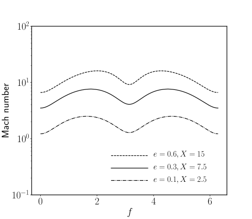
Figure 1.— Local Mach number versus true anomaly for a perturber in a Keplerian orbit with eccentricity $e$ embedded in a disk with constant aspect ratio $h=0.04$.

We define the local Mach number ${\mathcal{M}}$ as $V_{\rm rel}/c_{s,p}$, where $c_{s,p}$ is the disk sound speed at the position of the perturber. Figure 1 shows ${\mathcal{M}}$ for a disk with constant aspect ratio ($h=c_{s}/[\Omega R]=0.04$), for different values of $e$. The local minima of ${\mathcal{M}}$ occur at pericenter ($f=0$) and at apocenter ($f=\pi$). As noted by Muto et al. (2011) and Grishin & Perets (2015), perturbers move supersonically, at any point of the orbit, as long as $X>2$ (see Fig. 1). In the remainder of the paper, we will focus on cases with $X>2$.

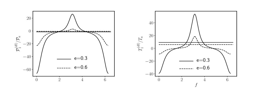
Figure 2.— Theoretical power (left) and torque (right) versus $f$ in the local approximation, for $e=0.3$ (solid lines) and $e=0.6$ (dashed lines). We take $\alpha=0$. The horizontal lines indicate their mean values averaged over time.

3. The local approximation

3.1. Migration and eccentricity damping

Consider first a strictly 2D sheet of gas (i.e. an infinitelly thin slab) with constant surface density $\Sigma_{0}$ and sound speed $c_{s}$. The slab, which is initially at rest, is perturbed by a moving body which interacts only gravitationally with the gaseous medium through the potential

$$\Phi_{p}=-\frac{GM_{p}}{\sqrt{s^{2}+R_{\rm soft}^{2}}},$$ (5)

where $s$ is the distance from the perturber. We assume that the perturber travels in a rectilinear trajectory at constant supersonic velocity, and denote by $\mbox{\boldmath$V$}{}_{\rm rel}$ the velocity of the gas relative to the perturber. Linear theory predicts that extended perturbers with softening radius $R_{\rm soft}$ and $V_{\rm rel}>c_{s}$ feel a dynamical friction force given by

$$\mbox{\boldmath$F$}{}_{\rm df}^{\scriptscriptstyle(2D)}\simeq\frac{\pi\Sigma_{0}G^{2}M_{p}^{2}}{R_{\rm soft}V_{\rm rel}^{3}}\mbox{\boldmath$V$}{}_{\rm rel}$$ (6)

(Muto et al. 2011). As long as the orbiter moves supersonically with respect to the gas and the softening radius keeps constant along the trajectory, $\mbox{\boldmath$F$}{}_{\rm df}$ does not depend on $c_{s}$.

Table 1Parameters of our reference 2D runs

All the simulations in this Table use the fiducial vaues: $\alpha=0$, $h=0.04$ and $\nu=\nu_{0}=10^{-5}\omega a^{2}$. Run $e$ ${\mathcal{E}}$ $R_{\rm in}$ $R_{\rm out}$ zones per $R_{\rm soft}$ $(N_{R}^{\rm peri},N_{\phi})$ 1L $0.1$ $0.6$ $0.4a$ $3.5a$ $(9,\,6.5)$ 1S $0.1$ $0.15$ $0.4a$ $3.5a$ $(3,\,2.5)$ 3La $0.3$ $0.6$ $0.35a$ $2.6a$ $(14,\,6)$ 3Lb $0.3$ $0.6$ $0.23a$ $3.9a$ $(14,\,6)$ 3Lc $0.3$ $0.6$ $0.175a$ $5.2a$ $(14,\,6)$ 3Ld $0.3$ $0.6$ $0.35a$ $5.2a$ $(14,\,6)$ 3S $0.3$ $0.15$ $0.23a$ $3.9a$ $(2.5,\,2)$ 6L $0.6$ $0.6$ $0.12a$ $4.5a$ $(12,\,4)$ 6S $0.6$ $0.15$ $0.175a$ $5a$ $(2.5,\,2)$

Now consider a perturber embedded in the disk in a Keplerian orbit. The local approximation consists in assuming that the interaction between a supersonic perturber and the disk can be described at every point of the orbit by Equation (6) just taking the surface density, sound speed and $\mbox{\boldmath$V$}{}_{\rm rel}$ at the position of the perturber (e.g., Muto et al., 2011; Grishin & Perets, 2015).

Once $\mbox{\boldmath$F$}{}_{\rm df}$ is known, we can evaluate the power ${\mathcal{P}}^{\rm(df)}_{1}$ and the torque $T^{\rm(df)}_{1}$, predicted in the local approximation, as a function of the true anomaly $f$. Combining Eqs. (3), (4) and (6), neglecting the pressure term as it is of order of ${\mathcal{O}}(h^{2})$, and using that $GM_{p}=q\omega^{2}a^{3}$, we find that

$${\mathcal{P}}^{\rm(df)}_{1}=\mbox{\boldmath$v$}{}_{p}\cdot\mbox{\boldmath$F$}{}_{\rm df}^{\scriptscriptstyle(2D)}=\frac{\pi\eta q^{2}\omega^{3}a^{5}\Sigma_{p}}{R_{\rm soft}}\frac{-e^{2}\sin^{2}f+\xi\hat{\xi}}{[e^{2}\sin^{2}f+\hat{\xi}^{2}]^{3/2}},$$ (7)

where $\Sigma_{p}$ is the unperturbed disk surface density at perturber’s location,

$$\xi(f)\equiv 1+e\cos f,$$ (8)

and

$$\hat{\xi}(f)=\sqrt{\xi}-\xi.$$ (9)

On the other hand, the torque is given by

$$T^{\rm(df)}_{1}=\hat{\mbox{\boldmath$e$}{}}_{z}\cdot(\mbox{\boldmath$r$}{}_{p}\times\mbox{\boldmath$F$}{}^{\scriptscriptstyle(2D)}_{\rm df})=\frac{\pi\eta^{4}q^{2}\omega^{2}a^{5}\Sigma_{p}}{R_{\rm soft}}\frac{\hat{\xi}}{\xi(e^{2}\sin^{2}f+\hat{\xi}^{2})^{3/2}}.$$ (10)

In the most general case, $R_{\rm soft}$ may depend on the position along the orbit. If so, it should be evaluated at the instantaneous position of the perturber. Once the power and the torque are known, the evolution of $a$ and $e$ can be computed using Equations (1) and (2).

We warn that, instead of ${\mathcal{P}}_{1}$, some authors provide the total power exerted by the accretion disk ${\mathcal{P}}_{\rm tot}={\mathcal{P}}_{d,0}+{\mathcal{P}}_{1}$, where ${\mathcal{P}}_{d,0}$ is the power associated with the radial force created by the (axisymmetric) unperturbed disk. As shown in the Appendix A, ${\mathcal{P}}_{\rm tot}$ and ${\mathcal{P}}_{1}$ exhibit different dependences on $f$. There are cases where ${\mathcal{P}}_{\rm tot}$ may be dominated by the contribution of ${\mathcal{P}}_{d,0}$. Nonetheless, ${\mathcal{P}}_{d,0}$ does not contribute to the change of the orbital elements (see Eqs. 1 and 2) because its value averaged over one orbit is zero.

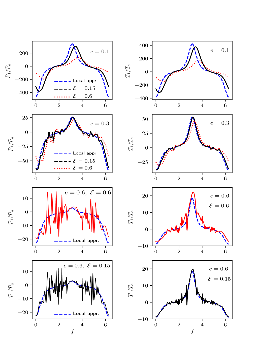
Figure 3.— Dimensionless power (left columns) and torque (right columns) versus the true anomaly on the 13th orbit, for different combinations of $e$ and $\mathcal{E}$. In all cases $\alpha=0$ and $h=0.04$. The value of $e$ is given in the upper right corner on each panel. Black lines represent the values obtained from 2D simulations with $\mathcal{E}=0.15$, while red lines correspond to $\mathcal{E}=0.6$. The predicted curves in the local approximation are indicated by the dashed blue lines. For clarity, the case with $e=0.6$ has been split in different panels.

Table 2Parameters of the complementary 2D runs

Run	$h$	$\alpha$	$e$	${\mathcal{E}}$	$R_{\rm in}$	$R_{\rm out}$	zones per $R_{\rm soft}$
							$(N_{R}^{\rm peri},N_{\phi})$
A	$0.04$	$0$	$0.15$	$0.6$	$0.23a$	$3.9a$	$(12,\,4)$
B	$0.04$	$0.5$	$0.6$	$0.6$	$0.12a$	$4.75a$	$(7.5,\,4)$
C	$0.04$	$1.5$	$0.15$	$0.6$	$0.4a$	$3.5a$	$(12,\,4)$
D	$0.04$	$1.5$	$0.3$	$0.6$	$0.23a$	$3.9a$	$(9.5,\,4)$
E	$0.04$	$1.5$	$0.6$	$0.15$	$0.12a$	$4.75a$	$(2,\,2)$
F	$0.1$	$0$	$0.6$	$0.24$	$0.2a$	$5a$	$(7.5,\,4)$
G	$0.1$	$0$	$0.6$	$0.6$	$0.2a$	$5a$	$(7.5,\,4)$

3.2. General considerations on the accuracy of the local approximation: open questions

The local approximation implicitly assumes that the major contribution to the force comes from material at distances $\ll R$ from the body. Therefore, radial gradients in the unperturbed surface density and sound speed of the disk are disregarded when calculating the structure of the wake. The local approximation also neglects the differential rotation of the disk and thereby resonant effects. Thus, it also ignores that for certain impact parameters, the streamlines are not supersonic relative to the perturber even if ${\mathcal{M}}>1$ (see Appendix B). Finally, the local approximation neglects the curvature of the wake and therefore it does not take into account that the perturber can catch its own wake.

A systematic study on the accuracy of the local approximation has not not been conducted so far. Even in razor thin disks, the range of parameters within which the local approximation is accurate has not been clearly established. One would expect that the local approximation overestimates the force because it ignores the curvature of the wake which is expected to reduce the magnitude of $F_{1}$ (e.g., Kim & Kim, 2007; Sánchez-Salcedo et al., 2018). However, a rough comparison with the simulations in Cresswell & Nelson (2006) indicates that the local approximation underestimates the torque by a factor of $2$ (see fig. 8 in Muto et al. 2011).

Muto et al. (2011) also noted that the behaviour of the power versus the orbital angle reported in Cresswell et al. (2007) is very different to the predicted profile and this leads them to conclude that the local approximation may result in an oversimplified model for $\mbox{\boldmath$F$}{}_{1}$. However, Muto et al. (2011) compared ${\mathcal{P}}_{1}$ with ${\mathcal{P}}_{t}$, which are not the same quantity (see Appendix A).

From the ongoing discussion, it is clear that a more fair comparison between simulations and predictions is needed to evaluate the accuracy of the local approximation. This will be carried out in the next section.

4. Numerical experiments

We have carried out a set of 2D simulations of a gaseous disk that is perturbed by a gravitational body using the code FARGO3D (Benítez-Llambay & Masset, 2016) in polar coordinates centered on the central mass $M_{c}$. The computational domain covers a ring with $R_{\rm in}\leq R\leq R_{\rm out}$ and $0\leq\phi\leq 2\pi$, where $R_{\rm in}$ and $R_{\rm out}$ are the inner and outer radii. At both inner and outer boundaries, we use wave damping boundary conditions (de Val-Borro et al., 2006). A locally isothermal equation of state is used, where the sound speed $c_{s}$ is a fixed function of radius; it is set out by requiring that the disk aspect ratio $h$ defined as $c_{s}/(\Omega R)$ is constant with $R$. We also employ a kinematic viscosity $\nu$ that is constant over the entire disk. In most of the models, $\nu=10^{-5}\omega a^{2}$. The unperturbed surface density of the disk follows a power law $\Sigma_{0}=\Sigma_{a}(R/a)^{-\alpha}$.

We consider a perturber in a fixed elliptical orbit with eccentricity $e$. The perturber’s gravitational potential is smoothed over a fraction $\mathcal{E}$ of the local value of $H$ (defined as $c_{s}/\Omega$), so that $\mathcal{E}\equiv R_{\rm soft}/H$ is constant along the orbit. No removal of mass near the perturber was implemented.

Our assumption that $\mathcal{E}$ is constant along the orbit is physically justified for perturbers moving in circular orbits (e.g., Masset, 2002; Müller et al., 2012), but this is not the case here. For elliptical orbits, one may consider to use a different dependence of $\mathcal{E}$ with the position and velocity of the perturber. Since the local approximation does not require any particular choice for $\mathcal{E}$, we will use this simplest assumption for the sake of concreteness.

We have performed calculations with different $\alpha$, $h$, $e$ and ${\mathcal{E}}$. The parameters of our fiducial models (i.e. those models with $\alpha=0$ and $h=0.04$) are compiled in Table 1. In these simulations, we vary only two parameters: the eccentricity between $0.1$ and $0.6$, and ${\mathcal{E}}$ between $0.15$ and $0.6$. We thus employ a mnemonic nomenclature for the runs using the number $e/0.1$, followed by S or L, indicating whether ${\mathcal{E}}$ is small (${\mathcal{E}}=0.15$) or large (${\mathcal{E}}=0.6$). For instance, Run 3L indicates that $e=0.3$ and ${\mathcal{E}}=0.6$. Other complementary models with different $\alpha$ or $h$ are listed in Table 2.

The value of the mass ratio $q$ was taken small enough so that the interaction is linear but not too small that the results could be affected by numerical noise. As a compromise, we adopted $q=10^{-5}$ in all simulations except Run 1S for which we took $q=2.5\times 10^{-6}$.

In all simulations, the number of zones per $R_{\rm soft}$ in the radial $N_{R}$ and azimuthal $N_{\phi}$ directions is at least $2$, at any point of the orbit. Since the zones are linearly spaced in $R$ and $\phi$, $N_{\phi}$ is independent of $R$, but $N_{R}$ varies with $R$, being lowest at pericenter with a value given in Tables 1 and 2.

Our aim is to compute ${\mathcal{P}}_{1}$ and $T_{1}$ in the simulations and compare them to the values ${\mathcal{P}}_{1}^{\rm(df)}$ and $T_{1}^{\rm(df)}$ derived in the local approximation. More specifically, the power and the torque were obtained from the simulations using ${\mathcal{P}}_{1}=\mbox{\boldmath$v$}{}_{p}\cdot\mbox{\boldmath$F$}{}_{1}$ and $T_{1}=\hat{\mbox{\boldmath$e$}{}}_{z}\cdot(\mbox{\boldmath$r$}{}_{p}\times\mbox{\boldmath$F$}{}_{1})$ with

$$\mbox{\boldmath$F$}{}_{1}=\int(\Sigma-\Sigma_{0})\mbox{\boldmath$\nabla$}{}\Phi_{p}\,dA,$$ (11)

where $dA$ is the surface element. We recall that $\Sigma_{0}$ is the unperturbed, i.e. the initial, surface density of the disk.

By using that $R_{\rm soft}=\mathcal{E}hR$ in our disk models, Equations (7) and (10) for the power and the torque can be written as

$${\mathcal{P}}^{\rm(df)}_{1}={\mathcal{P}}_{a}\xi^{1+\alpha}\frac{(-e^{2}\sin^{2}f+\xi\hat{\xi})}{(e^{2}\sin^{2}f+\hat{\xi}^{2})^{3/2}},$$ (12)

$$T^{\rm(df)}_{1}=\frac{\xi^{\alpha}\hat{\xi}T_{a}}{(e^{2}\sin^{2}f+\hat{\xi}^{2})^{3/2}},$$ (13)

where

$${\mathcal{P}}_{a}=\frac{\pi q^{2}\omega^{3}a^{4}\Sigma_{a}}{\eta^{1+2\alpha}\mathcal{E}h},$$ (14)

and

$$T_{a}=\frac{\pi\eta^{2(1-\alpha)}q^{2}\omega^{2}a^{4}\Sigma_{a}}{\mathcal{E}h}.$$ (15)

The dimensionless power ${\mathcal{P}}^{\rm(df)}_{1}/\mathcal{P}_{a}$ and torque $T_{1}^{\rm(df)}/T_{a}$ only depend on $\alpha$, $e$ and the orbital phase $f$. For illustration, Figure 2 shows ${\mathcal{P}}_{1}^{\rm(df)}$ and $T_{1}^{\rm(df)}$ as a function of $f$ for $\alpha=0$ and two values of $e$ ($0.3$ and $0.6$). Both ${\mathcal{P}}_{1}^{\rm(df)}$ and $T_{1}^{\rm(df)}$ are positive at apocenter ($f=\pi$) and negative at pericenter ($f=0$). This is because the gas rotates faster than the perturber at apocenter and pushes it (Cresswell et al., 2007; Muto et al., 2011). At pericenter, on the contrary, the perturber experiences a drag because it moves at a speed greater than the gas. We see that the mean values of the power over one orbit are small compared to their dynamical range. In the next section (§4.1), we examine whether the local approximation can account for the changes of ${\mathcal{P}}_{1}$ and $T_{1}$ along the orbit. Later, in §4.2, we check if the mean values over one orbit are consistent with the estimates in the framework of the local approximation.

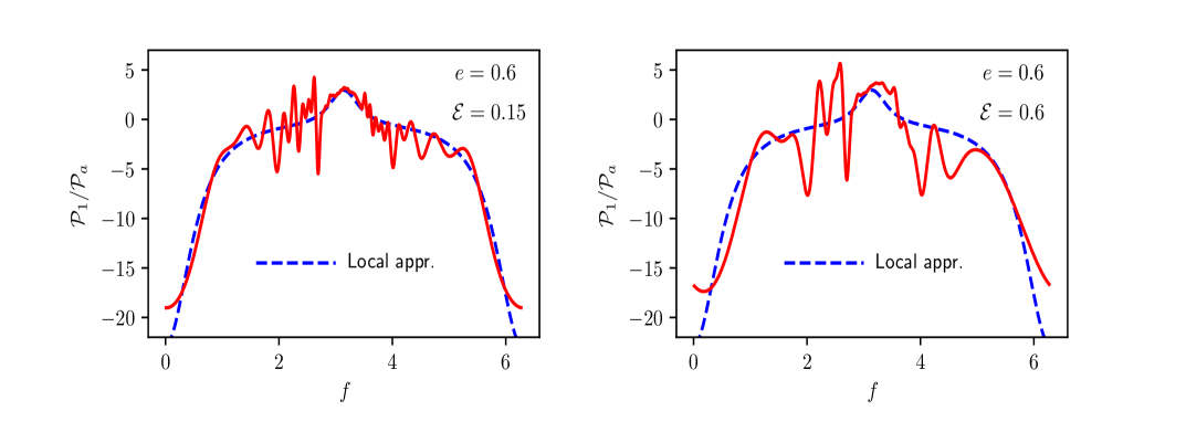
Figure 4.— Dimensionless power during the $13$th orbit in Run 6S (left) and Run 6L (right), after filtering out the high-frequency oscillations (solid lines). The dashed lines indicate the power estimated in the local approximation.

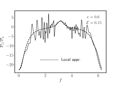
Figure 5.— Dimensionless power as a function of $f$, during the $13$th orbit, for a simulation with same parameters as Run 6S expect the viscosity, which is factor of $5$ larger. The dashed line indicates the theoretical values in the local approximation.

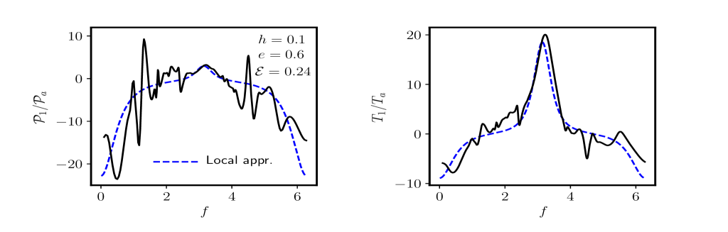
Figure 6.— Dimensionless power (left panel) and torque (right panel) during the $13$th orbit in Run F (solid lines). The dashed lines indicate the theoretical curves in the framework of the local approximation.

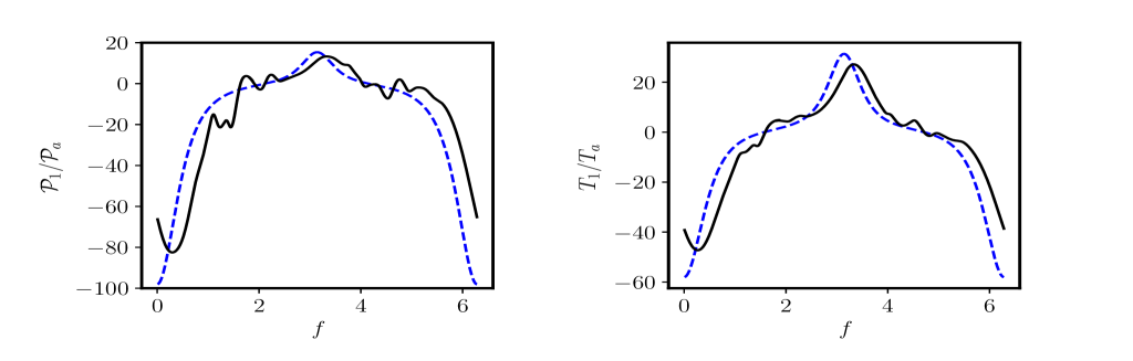
Figure 7.— Same as Figure 6 but for Run D.

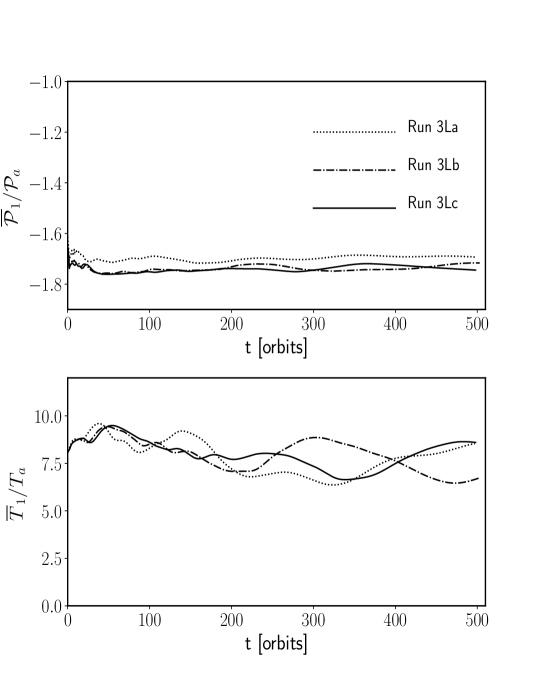
Figure 8.— Time evolution of $\overline{\mathcal{P}}_{1}$ and $\overline{T}_{1}$, in dimensionless units, for various sizes of the computational domain (see Table 1). The parameters of the disk, the eccentricity and the softening radius are the same in all cases ($h=0.04$, $e=0.3$, and ${\mathcal{E}}=0.6$).

4.1. Dependence of ${\mathcal{P}}_{1}$ and $T_{1}$ on the orbital phase

For clarity, we will first focus on the simulations of a disk with $\alpha=0$ (i.e. constant surface density at $t=0$) and $h=0.04$. Figure 3 shows ${\mathcal{P}}_{1}$ and $T_{1}$ versus $f$, for $e=0.1,0.3$ and $0.6$, which correspond to $X=2.5,7.5$ and $15$, respectively. The curves in Figure 3 were extracted when the perturber was completing the $13$th orbit.

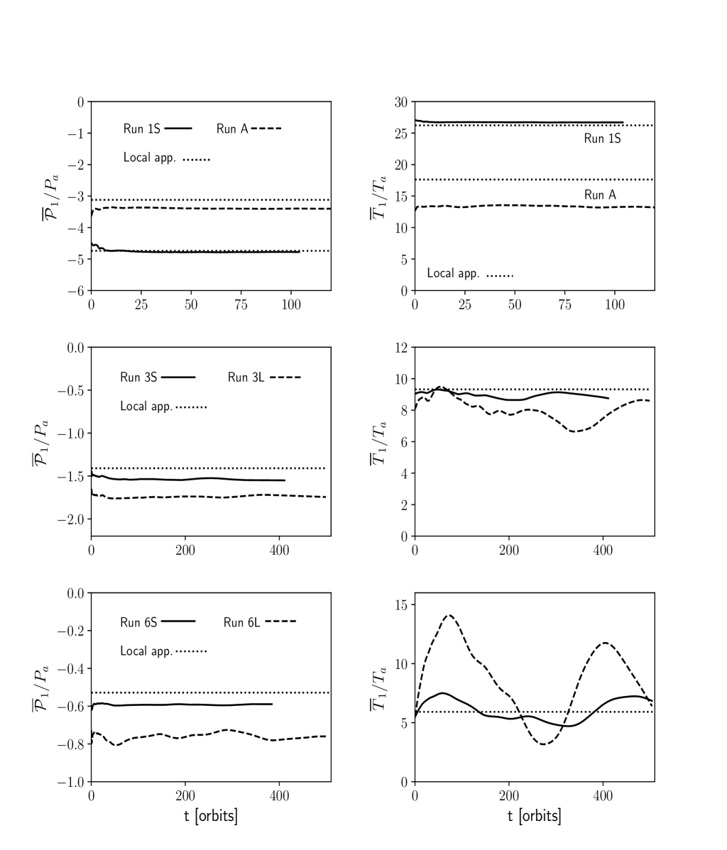
Figure 9.— Time evolution of $\overline{{\mathcal{P}}}_{1}$ (left column) and $\overline{T}_{1}$ (right column) for different combinations of $e$ and ${\mathcal{E}}$. The solid curves are for models with ${\mathcal{E}}=0.15$ and the dashed curves for ${\mathcal{E}}=0.6$. The horizontal dotted lines correspond to the predicted values in the local approximation. In all cases $\alpha=0$ and $h=0.04$.

In general, the differences between predictions and numerical results disminish as $\mathcal{E}$ decreases. The reason is simple; the relative contribution of the field in the vicinity of the body increases as $\mathcal{E}$ decreases. Therefore, the contribution of the far field, which is not captured well in the local approximation, becomes gradually less important relative to the contribution of the near field as $\mathcal{E}$ decreases.

For $e=0.1$ (i.e. $X=2.5$), the local approximation can reproduce neither the magnitude of the power nor the torque if $\mathcal{E}=0.6$. This is expected because the Mach $1$ distance is $\lesssim R_{\rm soft}$ (see Appendix B). We also see that the curves of ${\mathcal{P}}_{1}$ and $T_{1}$ are shifted with respect to the predicted curves for $\mathcal{E}=0.6$. If ${\mathcal{E}}$ is reduced a factor of $4$ (${\mathcal{E}}=0.15$), the curves match quite well each other if the predicted curves are shifted right by $\Delta f=0.33$. This shift has little effect when computing migration and eccentricity damping timescales because the averaged values over one orbit are preserved.

For $e=0.3$ (i.e. $X=7.5$), the local approximation predicts correctly ${\mathcal{P}}_{1}$ and $T_{1}$ for $\mathcal{E}=0.15$. Even for $\mathcal{E}=0.6$, the shapes of ${\mathcal{P}}_{1}$ and $T_{1}$ are captured well in the local approximation. At apocenter, the power and the torque are a bit lower than predicted. They also slightly deviate at pericenter.

For $e=0.6$ (i.e. $X=15$), $T_{1}$ but especially $\mathcal{P}_{1}$ exhibit spikes that are produced when the perturber crosses shock fronts and density substructures. These spikes are well-resolved in both strength and time, but they obscure the averaged value over a longer timescale. In order to make a better comparison with the values predicted by the local approximation, we use a time Fourier filter to remove high-frequency modes. Figure 4 shows that the filtered power for $e=0.6$ behaves in the manner predicted by the local approximation, even if ${\mathcal{E}}=0.6$.

A larger viscosity may smear the gradients in the velocity and may contribute to smooth the power and torque. Figure 5 shows the non-filtered power in a simulation similar to Run 6S except the viscosity was increased by a factor of $5$. The amplitude of the spikes reduces by a factor of $2$.

In order to illustrate the influence of the temperature of the disk on the abundance and amplitude of spikes, Figure 6 shows the power and the torque also for $e=0.6$, but $h=0.1$, implying $X=6$ (Run F in Table 2). This simulation has the same ${\mathcal{E}}h=0.024$ as Run 6L, and thereby they have the same softening radius. The level of substructure in ${\mathcal{P}}_{1}$ and $T_{1}$ is reduced as compared to Run 6L. A slight asymmetry with respect to $f=\pi$ is visible in both the power and the torque. The main discrepancy between simulations and the predicted values occurs for the power when the perturber is passing close to pericenter.

Finally, we have verified that the local approximation also predicts sucessfully the shape of ${\mathcal{P}}_{1}$ and $T_{1}$ for a disk with $\alpha=1.5$. As an example, Figure 7 shows the power and the torque for $e=0.3$ and $\alpha=1.5$ (Run D in Table 2).

In summary, we find that for ${\mathcal{E}}<0.6$, the local approximation reproduces qualitatively the dependence of ${\mathcal{P}}_{1}$ and $T_{1}$ with the orbital phase, after several orbits, provided that $X>3.75$. For values $X\simeq 2.5$, we need smaller values for ${\mathcal{E}}$. For $X\simeq 15$, the power presents remarkable spikes but still the local approximation can explain the underlying shape. In the next section, we carry out an analysis of the orbit averaged values of the power and the torque, and consider a longer timescale.

4.2. Averaged values of the power and torque over one orbital period: Long-term evolution

The relevant quantities to compute the orbital evolution of the perturbing object are $\overline{{\mathcal{P}}}_{1}$ and $\overline{T}_{1}$, where the over-bar indicates the average value over intervals of one orbital period. In analytical calculations, it is frequent to assume that all the quantities of the fluid are periodic with frequency $\omega$, i.e. the perturbation in the gas is the same in succesive passes of the body at the same position. Under this assumption, $\overline{{\mathcal{P}}}_{1}$ and $\overline{T}_{1}$ are independent of time.

For $h=0.04$, we find that $\overline{\mathcal{P}}_{1}$ and $\overline{T}_{1}$ maintain approximately constant along the simulation if $e<0.2$ (i.e. $X<5$). In general, however, they are not constant but display long-term variations. Such temporal changes may be genuine or a consequence of spurious boundary effects. In order to assess the effect of the limited size of the computational box, Figure 8 shows the time evolution of $\overline{\mathcal{P}}_{1}$ and $\overline{T}_{1}$ for our fiducial parameters ($\alpha=0$, $h=0.04$) with $e=0.3$, and ${\mathcal{E}}=0.6$ for various sizes of the domain, keeping the same resolution (Runs 3La, 3Lb and 3Lc in Table 1). We will focus on the behaviour of the torque because the differences in the power are ignorable. At $t<300$ orbits, the magnitude of the variations in the torque is least in the simulation with the largest radial extension (Run 3Lc); $\overline{T}_{1}/T_{a}$ varies gradually between $9.5$ at $40$ orbits to $8$ at $t=275$ orbits (a change of $16\%$). After $275$ orbits, the dimensionless torque in the three simulations oscillates between $6$ and $9$. Although we cannot rule out that, beyond $275$ orbits, part of the temporal variation of the torque is caused by boundary artifacts even in Run 3Lc, the mean value of $\overline{T}_{1}$ over the whole runtime is rather similar in the three simulations.

In Runs 3La, 3Lb and 3Lc, both $R_{\rm in}$ and $R_{\rm out}$ were varied. However, we have carried out simulations with the same $R_{\rm out}$, but with different $R_{\rm in}$ (from $0.17a$ to $0.35a$) and found that the oscillations in the torque are not very sensitive to $R_{\rm in}$ for values within that range. We have also found that the results are robust to reasonable changes in the size of the wave killing region in our damping conditions.

Figure 9 shows the temporal evolution of $\overline{\mathcal{P}}_{1}$ and $\overline{T}_{1}$ for $\alpha=0$, $h=0.04$ and different combinations of $e$ and ${\mathcal{E}}$. The horizontal lines correspond to the values predicted in the local approximation. The first result is that the agreement between simulations and theoretical estimates is reasonably good in all the cases when ${\mathcal{E}}=0.15$. In addition, for this value of ${\mathcal{E}}$, $\overline{T}_{1}$ is fairly constant over time for $e\leq 0.3$. For $e=0.6$, $\overline{T}_{1}$ varies around a value close to that predicted by the local approximation with a moderate amplitude.

For ${\mathcal{E}}=0.6$, $\overline{T}_{1}$ exhibits long-term variations of large amplitude if $e=0.6$ (Run 6L). These variations occur in a characteristic timescale of $\tau_{\rm var}\simeq 200$ orbits. The fact that the torque increases by a factor of $2.4$ in the first $75$ orbits suggests that the changes in $\overline{T}_{1}$ have a physical origin rather than being a numerical artifact. Figure 10 shows the torque as a function of the orbital phase during the $75$th and $274$th orbits, i.e. when the torque reaches a local maximum and a local minimum, respectively. The curves $T_{1}$ vs $f$ are now clearly asymmetric with respect to $f=\pi$; the torque when the perturber travels from pericenter to apocenter is different to when it goes from apocenter to pericenter. The variations in the torque are a consequence of the complexity of the far-field flow, which takes hundreds of orbits to achieve a periodic configuration for $e=0.6$.

We have run the same simulation (Run 6L) with viscosities between $0.2\times 10^{-5}$ and $5\times 10^{-5}$ (in units of $\omega a^{2}$) and found only a $10\%$ change in $\overline{T}_{1}$ after $300$ orbits. This is expected because the origin of the long-term fluctuations in the torque is related to the large-scale perturbations in the flow, which are unaffected by viscosity.

We have also computed the torque in simulations where the orbit is not fixed to be elliptical, but forms a rosette figure after including the potential associated with the unperturbed disk. In these simulations, the changes of $\overline{T}_{1}$ over time are similar.

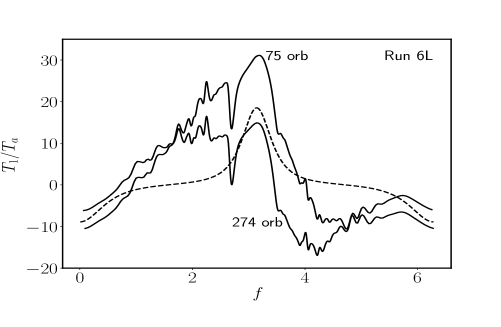
Figure 10.— Dimensionless torque over the $75$th orbit (upper solid curve), and the $274$th orbit (lower solid curve) for Run 6L ($e=0.6$ and ${\mathcal{E}}=0.6$). At these orbits, $\overline{T}_{1}$ presents a local maximum and minimum, respectively. For reference, the local approximation curve is also given (dashed line).

The amplitude of the temporal variations in $\overline{T}_{1}$ depend largely on $\alpha$ and $h$. In disks with larger values of $h$, the sound speed is larger and the amplitude of density perturbations in the disk are smeared out in a shorter timescale. For a model with $h=0.1$ and $e=0.6$ (Run F), $\overline{T}_{1}$ is essentially constant after $130$ orbits (see Figure 11).

Figure 12 shows the time evolution of $\overline{T}_{1}$ for two different values of $\alpha$ ($\alpha=0.5$ and $1.5$). Greater is the value of $\alpha$, higher is the amplitude of the variations in the torque. We warn that in the simulations with $\alpha=1.5$, our damping boundary conditions do not preserve mass over the runtime. For instance, in Run E, the mass contained within the apocenter radius increases by $22\%$ after $360$ orbits. A more delicate comparison should take into account this secular mass enhancement.

It is remarkable and worthwhile noting that at $t\lesssim 12$ orbits, the values of $\overline{T}_{1}$ in the simulations are fully consistent with those obtained in the framework of the local approximation, even in runs with ${\mathcal{E}}=0.6$ (see Figs. 9, 11 and 12).

4.3. The maximum softening radius

From our simulations, we can compute the mean value of the torque over the runtime $t_{\rm run}$ as

$$\left<\overline{T}_{1}\right>=\frac{1}{t_{\rm run}}\int_{0}^{t_{\rm run}}\overline{T}_{1}dt.$$ (16)

For models with large temporal variations in the torque, $\left<\overline{T}_{1}\right>$ is meaningful only if $t_{\rm run}$, $\tau_{a}$ and $\tau_{e}$ are $\gg\tau_{\rm var}$. Otherwise, one should consider the detailed temporal evolution of the power and the torque to find the evolution of the orbital parameters of the embedded object. Since $\tau_{e}\ll\tau_{a}$, the required condition is $\tau_{e}\gg\tau_{\rm var}\simeq 150$ orbits. Given that $\tau_{e}$ increases as $q$ decreases, this condition provides an upper limit value for $q$.

As we have seen in the previous section (§4.2), the amplitude of the variations in the power and the torque decreases as ${\mathcal{E}}$ decreases. In fact, for ${\mathcal{E}}$ small enough, $\overline{\mathcal{P}}_{1}$ and $\overline{T}_{1}$ converge to the values predicted in the local approximation and, in addition, the rms of $\overline{\mathcal{P}}_{1}$ and $\overline{T}_{1}$ also decrease. Consequently, given the disk parameters $\alpha$ and $h$, and the orbital eccentricity, there exists a maximum value of $\mathcal{E}$, denoted by $\mathcal{E}_{\rm max}^{(2D)}$, such that if $\mathcal{E}<\mathcal{E}_{\rm max}^{(2D)}$ then (1) the local approximation provides the mean power and torque with an error less than $20\%$, and (2) the rms value of $\overline{T}_{1}$ is less than $0.15\left<\overline{T}_{1}\right>$. If conditions (1) and (2) are met, the local approximation shall be deemed satisfactory. In Table 3, we provide the values of $\mathcal{E}_{\rm max}^{(2D)}$ for different disk parameters and orbital eccentricities.

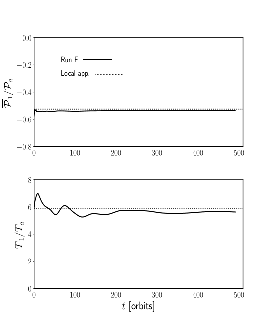
Figure 11.— Time evolution of $\overline{\mathcal{P}}_{1}$ (top panel) and $\overline{T}_{1}$ (bottom panel), in dimensionless units, for model F. The dotted lines indicate the theoretical values in the local approximation.

Table 3${\mathcal{E}}_{\rm max}^{(2D)}$ and ${\mathcal{E}}_{\rm max}^{(3D)}$ for some disk parameters and eccentricities

$h$	$\alpha$	$e$	${\mathcal{E}}_{\rm max}^{(2D)}$	${\mathcal{E}}_{\rm max}^{(3D)}$
$0.04$	$0$	$0.1$	$0.25$	$0.12$
$0.04$	$0$	$0.15$	$0.45$	$0.34$
$0.04$	$0$	$0.3$	$0.6$	$0.46$
$0.04$	$0$	$0.6$	$0.15$	$0.078$
$0.04$	$0.5$	$0.6$	$0.1$	$0.01$
$0.04$	$1.5$	$0.3$	$0.24$	$0.12$
$0.04$	$1.5$	$0.6$	$0.06$	$8\times 10^{-4}$
$0.1$	$0$	$0.6$	$0.7$	$0.6$

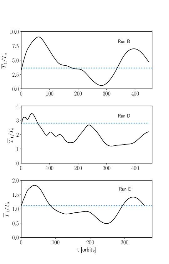
Figure 12.— Time evolution of $\overline{T}_{1}/T_{a}$ for models with $\alpha=0.5$ (top panel) and $\alpha=1.5$ (middle and bottom panels). The horizontal dotted lines show the predicted values adopting the local approximation.

Along this section, we have implicitly assumed that the accretion radius of the perturber $R_{\rm acc}\equiv GM_{p}/V_{\rm rel}^{2}$ is smaller than $R_{\rm soft}$ so that the perturbation is linear at any position, even at the vicinity of the perturber. In the case that $R_{\rm soft}<R_{\rm acc}$ then the relevant radius is not longer $R_{\rm soft}$ but $R_{\rm acc}$ (e.g., Bernal & Sánchez-Salcedo, 2013) and thereby the condition for the local approximation to be valid is $R_{\rm acc}<{\mathcal{E}}_{\rm max}^{(2D)}H$.

All the above considerations were depicted for a softened perturber embedded in a razor-thin disk. In the next Section, we extend the analysis of the applicability of the local approximation to a more realistic 3D disk and also to accreting perturbers.

5. Local approximation in 3D disks

The extension of the drag force, $F_{\rm df}^{(3D)}$, to a plane-parallel slab with finite thickness was derived in Cantó et al. (2013). They assume that the perturber moves in rectilinear trajectory in the midplane of a vertically stratified slab with density $\rho(z)=\rho_{0}\exp(-z^{2}/2H^{2})$. For a nonaccreting perturber with softening radius much smaller than $H$, they infer that

$$F^{\scriptscriptstyle(3D)}_{\rm df}=\frac{\sqrt{8\pi}\Sigma(GM_{p})^{2}}{V^{2}_{\rm rel}H}\ln\left(\frac{1.32H}{R_{\rm soft}}\right)$$ (17)

(see Sánchez-Salcedo et al., 2018, for details).

Since numerical simulations of a perturber in eccentric orbit embedded in a 3D disk are computationally expensive, it is useful to derive under which conditions the local approximation, using $F_{\rm df}^{(3D)}$, is appropriate to describe the interaction between a perturber and a 3D disk.

In §4.1 and 4.2, we found that if $R_{\rm soft}\leq\stackrel{{\scriptstyle\sim}}{{\smash{R}\rule{0.0pt}{4.73611pt}}}_{\rm soft}^{(2D)}\equiv{\mathcal{E}}_{\rm max}^{(2D)}H$, the local approximation in a 2D disk is reasonably accurate because the near wake region of the perturber, defined as the region in the vicinity of the perturber that is not affected by curvature terms, contributes to $80\%$ of the drag force or more. The near wake region in a 2D slab has a size $\simeq 5\stackrel{{\scriptstyle\sim}}{{\smash{R}\rule{0.0pt}{4.73611pt}}}_{\rm soft}^{(2D)}$.

In a disk with finite thickness, we also expect that the local approximation should be valid for sufficiently small perturbers, say $R_{\rm soft}\leq\stackrel{{\scriptstyle\sim}}{{\smash{R}\rule{0.0pt}{4.73611pt}}}_{\rm soft}^{(3D)}$. We can estimate $\stackrel{{\scriptstyle\sim}}{{\smash{R}\rule{0.0pt}{4.73611pt}}}_{\rm soft}^{(3D)}$ by imposing that the material within the near wake region contributes more than $80\%$ of the total drag. As curvature terms are a pure 2D effect, the near wake region is the same as in the 2D case. Therefore, $\stackrel{{\scriptstyle\sim}}{{\smash{R}\rule{0.0pt}{4.73611pt}}}_{\rm soft}^{(3D)}$ satisfies

$$F_{\rm df}^{(3D)}\bigg{|}_{\stackrel{{\scriptstyle\sim}}{{\smash{R}\rule{0.0pt}{3.31529pt}}}_{\rm soft}^{(3D)}}=5f_{\rm df}^{(3D)}\bigg{|}_{5\stackrel{{\scriptstyle\sim}}{{\smash{R}\rule{0.0pt}{3.31529pt}}}_{\rm soft}^{(2D)}},$$ (18)

where $f_{\rm df}^{(3D)}(r)$ is the drag force arising from material beyond a distance $r$ from the perturber. Following Cantó et al. (2013), we have computed $f_{\rm df}^{(3D)}(r)$ (see top panel of Figure 13), and then obtained ${\mathcal{E}}_{\rm max}^{(3D)}$ as a function of ${\mathcal{E}}_{\rm max}^{(2D)}$ (bottom panel in Figure 13). We see that ${\mathcal{E}}_{\rm max}^{(3D)}<{\mathcal{E}}_{\rm max}^{(2D)}$, i. e. the local approximation in a 3D disk requires even smaller perturbers than in a 2D disk.

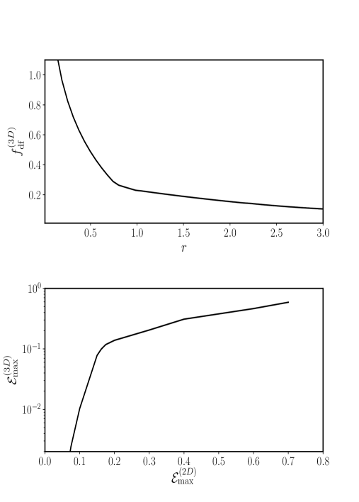
Figure 13.— Drag force on a perturber embedded in a vertically-stratified plane-parallel medium, arising from the enhanced-density wake at distances greater than $r$ from the perturber, in arbitrary units (top panel). Relationship between ${\mathcal{E}}_{\rm max}^{(2D)}$ and ${\mathcal{E}}_{\rm max}^{(3D)}$ (bottom panel).

For a point-like perfect accretor such as a black hole, the drag force including the aerodynamical drag due to accretion is, in the local approximation,

$$F_{\rm df}^{(3D)}=\frac{\sqrt{8\pi}\Sigma(GM_{p})^{2}}{V^{2}_{\rm rel}H}\ln\left(\frac{7.15H}{R_{\rm acc}}\right)$$ (19)

(Cantó et al., 2013). This formula is very similar to Equation (17) except the numerical value of the factor in the logarithm, which is larger in the case of a perfect accretor, reflecting the fact that accretion contributes to the drag force. Therefore, we are certain that the local approximation will be satisfactory if $R_{\rm acc}<\stackrel{{\scriptstyle\sim}}{{\smash{R}\rule{0.0pt}{4.73611pt}}}_{\rm soft}^{(3D)}$.

As the accretion radius is given by $R_{\rm acc}\equiv 2GM_{p}/V_{\rm rel}^{2}$, its maximum occurs at apocenter, when $V_{\rm rel}$ reaches its minumum value. At apocenter, $V_{\rm rel}\simeq e\omega a/[2(1+e)^{1/2}]$ and, thus, $R_{\rm acc}\simeq 8(1+e)qa/e^{2}$, where we have used that $GM_{p}=q\omega^{2}a^{3}$. Hence, the condition $R_{\rm acc}<\stackrel{{\scriptstyle\sim}}{{\smash{R}\rule{0.0pt}{4.73611pt}}}_{\rm soft}^{(3D)}$ can be cast in terms of $q$ as

$$q\lesssim\frac{e^{2}{\mathcal{E}}_{\rm max}^{(3D)}h}{8(1+e)}.$$ (20)

For illustration, in the following we discuss some relevant cases; the values used for ${\mathcal{E}}_{\rm max}^{(3D)}$ are given in Table 3. Consider a point-like perturber with $e=0.3$ embedded in a disk with $\alpha=0$ and $h=0.04$. The local approximation will have an accuracy better than $20\%$ if $q\lesssim 1.5\times 10^{-4}$, where we have used ${\mathcal{E}}_{\rm max}^{(3D)}=0.46$ in this case. It is interesting to compare this upper value with $q_{\rm crit}$ defined in Section 2. The simulations of Hosseinbor et al. (2007) indicate that $q_{\rm crit}\gg 10^{-4}$ for $e>0.2$. Therefore, for $e=0.3$, an accretor with a mass in the range $1.5\times 10^{-4}<q<q_{\rm crit}$ satisfies the type I condition but the local approximation might not be accurate.

Analogously, for $\alpha=0$, $h=0.04$ and $e=0.6$, we have ${\mathcal{E}}_{\rm max}^{(3D)}=0.08$, and Equation (20) implies $q\lesssim 0.8\times 10^{-4}$. For a thicker disk with $h=0.1$, we obtain $q\lesssim 1.5\times 10^{-3}$ (again for $\alpha=0$ and $e=0.6$).

6. Conclusions

In this paper, we have investigated the quality of the local approximation to estimating the tidal force acting on low-mass perturbers on eccentric orbits embedded in gaseous disks. To this aim, we have carried out 2D simulations of perturbers on fixed eccentric orbits with eccentricities between $0.1$ and $0.6$ in disks with constant aspect ratios ranging between $0.04$ and $0.1$. In all our simulations, the smoothing length of the perturber is larger than the accretion radius.

We find that the local approximation is good if (1) the parameter $X=e/h$ is larger than $2.5$ so that the perturber moves supersonically relative to the gas and (2) the softening radius is smaller than a certain threshold value $\stackrel{{\scriptstyle\sim}}{{\smash{R}\rule{0.0pt}{4.73611pt}}}_{\rm soft}$ so that the force contribution of the far-field, which is not well captured in the local approximation, is small. Since we are in the regime $R_{\rm acc}<R_{\rm soft}$, an upper value on $R_{\rm soft}$ implies an upper value on $q$.

We have first studied the short-term evolution, that is, when the companion has completed around $12$ orbits. At those times and for an aspect ratio typical in a protoplanetary disk $h=0.04$, the local approximation can reproduce pretty well both the power and the torque as a function of the orbital phase for a value of ${\mathcal{E}}\leq 0.15$. The mean values of the power and the torque over one orbit are well predicted in the local approximation.

On a longer timescale, some models exhibit temporal variations in the torque because the disk does not reach a periodic configuration in the runtime of our simulations ($\sim 400$ orbits). These variations occur on a characteristic timescale $\tau_{\rm var}$ of $\sim 150$ orbits. In some models, the amplitude of these variations is remarkable. For instance, for $\alpha=0$ and $R_{\rm soft}=0.024R$, the amplitude of the oscillations is comparable to the mean value if $X>12$. In those models that display such large amplitudes, the local approximation still predicts the force during the first stage of the run, at $t\lesssim 15$ orbits, but it obviously fails to account for the subsequent changes in the force. Hence, for those models, the local approximation can be applied if $q$ is large enough that $\tau_{e}\ll\tau_{\rm var}$.

The amplitude of these variations increases with $\alpha$, $X$ and $R_{\rm soft}$. Given $\alpha$ and $X$, the amplitude of the changes in the torque can be reduced by decreasing $R_{\rm soft}$. By imposing an upper limit on the amplitude of these torque fluctuations, we have established the threshold value $\stackrel{{\scriptstyle\sim}}{{\smash{R}\rule{0.0pt}{4.73611pt}}}_{\rm soft}^{(2D)}$ for the local approximation to be faithful.

An extension of the formula for the drag force in the local approximation that incorporates the vertical structure of the disk was proposed by Cantó et al. (2013). We have been able to determine the validity domain of the 3D local approximation. We have found the corresponding threshold softening radius $\stackrel{{\scriptstyle\sim}}{{\smash{R}\rule{0.0pt}{4.73611pt}}}_{\rm soft}^{(3D)}$ in the 3D case.

In the case of point-like perturbers, the relevant length is the accretion radius. In order for the 3D local approximation to be valid in this case, the accretion radius is required to satisfy $R_{\rm acc}\leq\stackrel{{\scriptstyle\sim}}{{\smash{R}\rule{0.0pt}{4.73611pt}}}_{\rm soft}^{(3D)}$. This condition imposes an upper limit to the value of $q$. In the case of thin disks ($h\simeq 0.04$) with $0\leq\alpha\leq 1/2$, we have found that, for objects with $q\lesssim 10^{-5}$, the 3D local approximation can be used to determine the orbital evolution in the entire range of orbital eccentricities considered (i.e. $e\in[0.1,0.6]$). This mass range includes the extreme mass-ratios inspirals of BHs in active galactic nuclei (e.g. Kocsis et al., 2011). It also includes planetary cores and embryos up to $3$ Earth masses in their natal protoplanetary disks. For thicker disks, the eccentricity range of validity is shifted towards larger values.

Appendix A A. Contribution of the background disk to the power: Mestel disk

The unperturbed disk is assumed to be axisymmetric. As a result, the unperturbed disk cannot create a torque on the orbiting body. However, it can induce a power for bodies with orbital eccentricity. The power arising from the unperturbed disk is denoted by ${\mathcal{P}}_{d,0}$ and it is given by

$${\mathcal{P}}_{d,0}=\mbox{\boldmath$v$}{}_{p}\cdot\mbox{\boldmath$F$}{}_{d,0},$$ (A1)

where $\mbox{\boldmath$v$}{}_{p}$ is the velocity of the body and $\mbox{\boldmath$F$}{}_{d,0}$ is the forced exerted on the body by the unperturbed disk. For concreteness, we focus on a Mestel disk, whose density decays with $R$ as $\Sigma(R)=\Sigma_{a}a/R$, where $a$ is the semimajor axis and $\Sigma_{a}$ is the surface density at $R=a$. The gravitational attraction between the unperturbed disk and a body located at a radius $r_{p}$ is

$$\mbox{\boldmath$F$}{}_{d,0}=-\frac{2\pi G\Sigma_{0}R_{0}M_{p}}{r_{p}}\hat{\mbox{\boldmath$e$}{}}_{r},$$ (A2)

where we have assumed $r_{p}\gg R_{\rm soft}$. For a body in quasi-Keplerian orbit with semimajor axis $a$ and eccentricity $e$, the power ${\mathcal{P}}_{d,0}$ as a function of $f$ can be written as

$${\mathcal{P}}_{d,0}=-\frac{2\pi peq\omega^{3}a^{4}\Sigma_{a}}{\eta^{3}}\sin f\,(1+e\cos f).$$ (A3)

Here we have used that $GM_{p}\simeq q\omega^{2}a^{3}$. As expected, for a circular orbit ${\mathcal{P}}_{d,0}=0$ and thus ${\mathcal{P}}_{\rm tot}={\mathcal{P}}_{1}$. In the following we will focus on eccentric orbits.

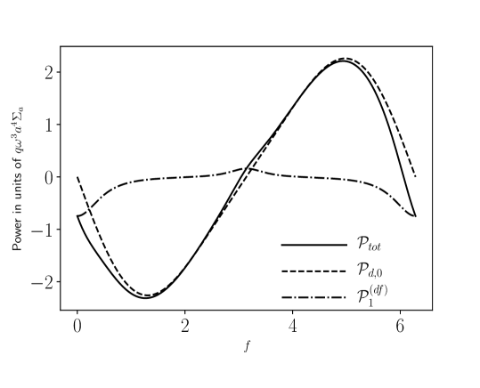
Figure 14.— Energy change per unit of time (power) as a function of the true anomaly for an orbit with $e=0.3$ in a Mestel disk with $h=0.05$. The pertuber has $q=6\times 10^{-5}$ and $R_{\rm soft}=0.6H$. The dashed line represents the contribution ${\mathcal{P}}_{d,0}$, the dot-dashed line indicates ${\mathcal{P}}^{\rm(df)}_{1}$ and the solid line is ${\mathcal{P}}_{\rm tot}$, i.e. the sum of both contributions.

Figure 14 shows ${\mathcal{P}}_{d,0}$, ${\mathcal{P}}^{\rm(df)}_{1}$ (from Equation 7) and ${\mathcal{P}}_{\rm tot}={\mathcal{P}}_{d,0}+{\mathcal{P}}^{\rm(df)}_{1}$ for a Mestel disk with $h=0.05$ and a perturber with $q=6\times 10^{-5}$, $e=0.3$ and $R_{\rm soft}=0.6H$. These values are the same as in (Cresswell et al., 2007) to facilitate comparison. It is apparent that the contribution of ${\mathcal{P}}^{\rm(df)}_{1}$ is disguised if we look at ${\mathcal{P}}_{\rm tot}$. Although ${\mathcal{P}}^{\rm(df)}_{1}$ appears to be much smaller in amplitude than ${\mathcal{P}}_{d,0}$, it is the relevant part of the power that determines the orbital evolution of the particle. In fact, ${\mathcal{P}}_{d,0}$ does not contribute to the change of the orbital elements because $\mathcal{P}_{d,0}=0$. It is also important to notice that ${\mathcal{P}}_{d,0}$ depends linearly on $q$, while ${\mathcal{P}}^{\rm(df)}_{1}$ depends quadratically. Therefore, the contribution of ${\mathcal{P}}_{d,0}$ relative to ${\mathcal{P}}^{\rm(df)}_{1}$ decreases as $q$ increases.

Appendix B B. The Mach $1$ distance

At apocenter, the local gas rotates at a velocity larger than the perturber. Since the circular velocity of the gas declines with $R$, there exists a distance in the outer disk (i.e. at $R>[1+e]a$) beyond which the relative velocity between a patch of gas and the perturber comes subsonic. In a disk with constant $h$, the Mach 1 distance $\Delta_{1}$ at apocenter is

$$\Delta_{1}^{(\rm apo)}=(1+e)a\left[\frac{1}{(\sqrt{1-e}+h)^{2}}-1\right].$$ (B1)

At pericenter, the orbiter rotates supersonically with respect to the local gas. However, at a distance

$$\Delta_{1}^{(\rm peri)}=(1-e)a\left[1-\frac{1}{(\sqrt{1+e}-h)^{2}}\right]$$ (B2)

interior to the perturber orbit, the relative velocity is $\simeq c_{s}$. For $e=0.3$ and $h=0.04$, we have that $\Delta_{1}^{(\rm apo)}=0.39a=7.5H_{\rm apo}$ and $\Delta_{1}^{(\rm peri)}=0.12a=4.3H_{\rm peri}$, where $H_{\rm apo}$ and $H_{\rm peri}$ are the scaleheight of the disk at apocenter and pericenter, respectively. This implies that the typical scale where the relative motion is supersonic is $\gtrsim 4H$, as long as $e\geq 0.3$. For $e=0.1$, we find that $\Delta_{1}^{(\rm apo)}=0.43H_{\rm apo}$ and $\Delta_{1}^{(\rm peri)}=0.58H_{\rm peri}$.

References

- Artymowicz (1994) Artymowicz, P. 1994, ApJ, 423, 581
- Baruteau et al. (2014) Baruteau, C., Crida, A., Paardekooper, S.-J., Masset, F., Guilet, J., Bitsch, B., Nelson, R., Kley, W., & Papaloizou, J. 2014, Protostars and Planets VI, Henrik Beuther, Ralf S. Klessen, Cornelis P. Dullemond, and Thomas Henning (eds.), University of Arizona Press, Tucson, 914 pp., p.667-689
- Benítez-Llambay & Masset (2016) Benítez-Llambay, P., & Masset, F. S. 2016, ApJS, 223, 11
- Bernal & Sánchez-Salcedo (2013) Bernal, C. G., & Sánchez-Salcedo, F. J. 2013, ApJ, 775, 72
- Bitsch & Kley (2010) Bitsch, B., & Kley, W. 2010, A&A, 523, 30
- Bitsch & Kley (2011) Bitsch, B., & Kley, W. 2011, A&A, 530, 41
- Bitsch et al. (2013) Bitsch, B., Crida, A., Libert, A.-S., & Lega, E. 2013, A&A, 555, 124
- Cantó et al. (2013) Cantó, J., Esquivel, A., Sánchez-Salcedo, F. J., & Raga, A. C. 2013, ApJ, 762, 21
- Cresswell & Nelson (2006) Cresswell, P., & Nelson, R. P. 2006, A&A, 450, 833
- Cresswell et al. (2007) Cresswell, P., Dirksen, G., Kley, W., & Nelson, R. P. 2007, A&A, 473, 329
- de Val-Borro et al. (2006) de Val-Borro, M., Edgar, R. G., Artymowicz, P., et al. 2006, MNRAS, 370, 529
- Duffell & Chiang (2015) Duffell, P. C., & Chiang, E. 2015, ApJ, 812, 94
- Fendyke & Nelson (2014) Fendyke, S. M., & Nelson, R. P. 2014, MNRAS, 437, 96
- Goldreich & Tremaine (1980) Goldreich, P., & Tremaine, S. 1980, ApJ, 241, 425
- Goldreich & Sari (2003) Goldreich, P., & Sari, R. 2003, ApJ, 585, 1024
- Grishin & Perets (2015) Grishin, E., & Perets, H. B. 2015, ApJ, 811, 54
- Hosseinbor et al. (2007) Hosseinbor, A. P., Edgar, R. G., Quillen, A. C., & LaPage, A. 2007, MNRAS, 378, 966
- Just & Peñarrubia (2005) Just, A., & Peñarrubia, J. 2005, A&A, 431, 861
- Kocsis et al. (2011) Kocsis, B., Yunes, N., & Loeb, A. 2011, PRD, 84, 024032
- Kim & Kim (2007) Kim, H., & Kim, W.-T. 2007, ApJ, 665, 432
- Marcy et al. (2005) Marcy, G., Butler, R. P., Fischer, D., Vogt, S., Wright, J. T., Tinney, C. G., & Jones, H. R. A. 2005, Prog. Theo. Physics Supp., 158, 24
- Marzari & Nelson (2009) Marzari, F., & Nelson, A. F. 2009, ApJ, 705, 1575
- Masset (2002) Masset, F. 2002, A&A, 387, 605
- Mills et al. (2019) Mills, S. M., Horward, A. W., Petigura, E. A., Fulton, B. J., Isaacson, H., & Weiss, L. M. 2019, AJ, 157, 198
- Müller et al. (2012) Müller, T. W. A., Kley, W., & Meru, F. 2012, A&A, 541, 123
- Muto et al. (2011) Muto, T., Takeuchi, T., & Ida, S. 2011, ApJ, 737, 37
- Papaloizou (2002) Papaloizou, J. C. B. 2002, A&A, 388, 615
- Papaloizou & Larwood (2000) Papaloizou, J. C. B., & Larwood, J. D. 2000, MNRAS, 315, 823
- Ragusa et al. (2018) Ragusa, E., Rosotti, G., Teyssandier, J., Booth, R., Clarke, C. J., & Lodato, G. 2018, MNRAS, 474, 4460
- Rein (2012) Rein, H. 2012, MNRAS, 422, 3611
- Sánchez-Salcedo & Brandenburg (2001) Sánchez-Salcedo, F. J., & Brandenburg, A. 2001, MNRAS, 322, 67
- Sánchez-Salcedo et al. (2018) Sánchez-Salcedo, F. J., Chametla, R. O., & Santillán, A. 2018, ApJ, 860, 129
- Tamuz et al. (2008) Tamuz, O., Ségransan, D., Udry, S., et al. 2008, A&A, 480, L33
- Tanaka & Ward (2004) Tanaka, H., & Ward, W. R. 2004, ApJ, 602, 388
- Udry & Santos (2007) Udry, S., & Santos, N. C. 2007, ARA&A, 45, 397
- Wittenmyer et al. (2007) Wittenmyer, R. A., Endl, M., Cochran, W. D., & Levison, H. F. 2007, AJ, 134, 1276
- Xie et al. (2016) Xie, J.-W., Dong, S., Zhu, Z., et al. 2016, Proceedings of the National Academy of Sciences of the United States of America, 113, 11431